1 SOLUTION OF Partial Differential Equations (PDEs) Mathematics is the Language of Science PDEs are the expression of processes that occur across time & space: (x,t), (x,y), (x,y,z), or (x,y,z,t)
Transcript
1
SOLUTION OF
Partial Differential Equations
(PDEs)
Mathematics is the Language of Science
PDEs are the expression of processes that occur across time & space: (x,t), (x,y), (x,y,z), or (x,y,z,t)
2
Partial Differential Equations (PDE's)
A PDE is an equation which includes derivatives of an unknown function with respect to 2 or more
independent variables
3
Partial Differential Equations (PDE's)PDE's describe the behavior of many engineering phenomena:
– Wave propagation– Fluid flow (air or liquid)
Air around wings, helicopter blade, atmosphereWater in pipes or porous mediaMaterial transport and diffusion in air or waterWeather: large system of coupled PDE's for momentum,
pressure, moisture, heat, …– Vibration– Mechanics of solids:
stress-strain in material, machine part, structure– Heat flow and distribution– Electric fields and potentials– Diffusion of chemicals in air or water– Electromagnetism and quantum mechanics
4
Partial Differential Equations (PDE's)
Weather Prediction• heat transport & cooling• advection & dispersion of moisture• radiation & solar heating• evaporation• air (movement, friction, momentum, coriolis forces)• heat transfer at the surface
To predict weather one need "only" solve a very large systems ofcoupled PDE equations for momentum, pressure, moisture, heat, etc.
5
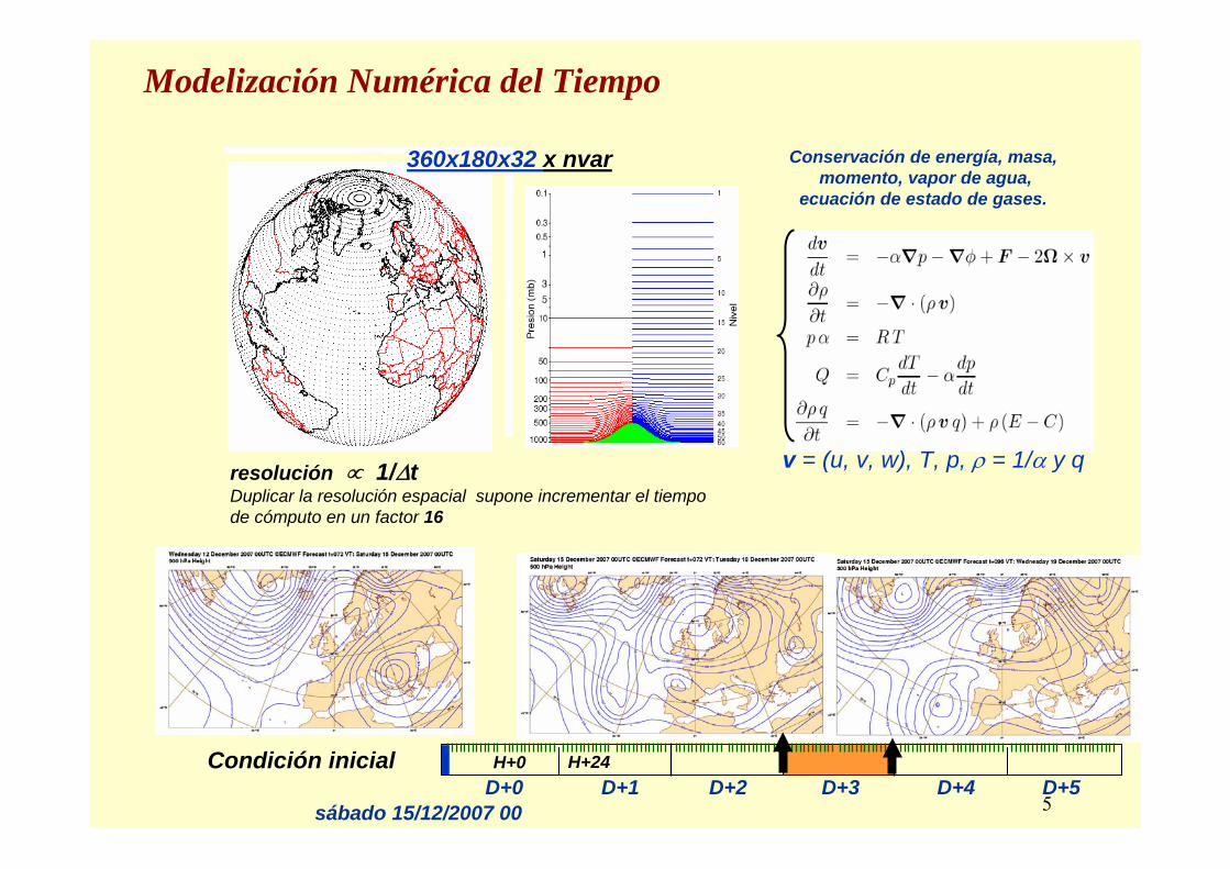
Conservación de energía, masa, momento, vapor de agua,
ecuación de estado de gases.
v = (u, v, w), T, p, ρ = 1/α y q
360x180x32 x nvar
resolución ∝ 1/ΔtDuplicar la resolución espacial supone incrementar el tiempo de cómputo en un factor 16
Modelización Numérica del Tiempo
D+0 D+1 D+2Condición inicial H+0 H+24
D+3 D+4 D+5sábado 15/12/2007 00
6
Partial Differential Equations (PDE's)
Learning Objectives
1) Be able to distinguish between the 3 classes of 2nd order, linear PDE's. Know the physical problems each class represents and the physical/mathematical characteristics of each.
2) Be able to describe the differences between finite-difference and finite-element methods for solving PDEs.
3) Be able to solve Elliptical (Laplace/Poisson) PDEs using finite differences.
4) Be able to solve Parabolic (Heat/Diffusion) PDEs using finite differences.
7
Partial Differential Equations (PDE's)Engrd 241 Focus:Linear 2nd-Order PDE's of the general form
u(x,y), A(x,y), B(x,y), C(x,y), and D(x,y,u,,)
The PDE is nonlinear if A, B or C include u, ∂u/∂x or ∂u/∂y, or if D is nonlinear in u and/or its first derivatives.
• Each category describes different phenomena.• Mathematical properties correspond to those phenomena.
2 2 2
2 2u u uA B C D 0
x yx y∂ ∂ ∂
+ + + =∂ ∂∂ ∂
8
Partial Differential Equations (PDE's)
Typical examples include
u u uu(x, y), (in terms of and )x y
∂ ∂ ∂∂ η ∂ ∂
Elliptic Equations (B2 – 4AC < 0) [steady-state in time]• typically characterize steady-state systems (no time derivative)
– temperature – torsion– pressure – membrane displacement– electrical potential
• closed domain with boundary conditions expressed in terms of
A = 1, B = 0, C = 1 ==> B2 – 4AC = – 4 < 0
2 22
2 2
0u uu u uD(x, y,u, , )x y x y
⎧∂ ∂ ⎪∇ ≡ + = ∂ ∂⎨−∂ ∂ ⎪ ∂ ∂⎩
Laplace Eq. Poisson Eq.
9
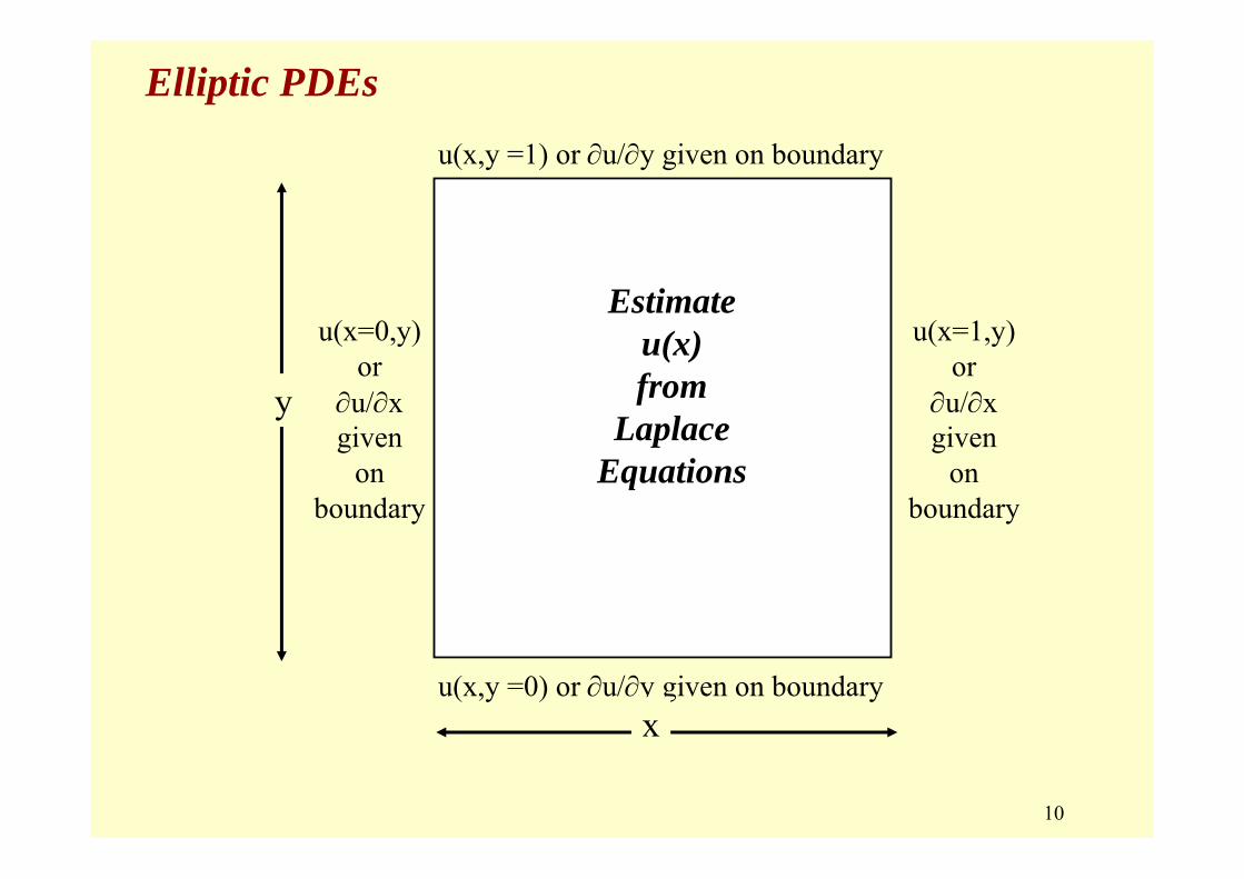
Elliptic PDEs Boundary Conditions for Elliptic PDE's:
Dirichlet: u provided along all of edge
Neumann: provided along all of the edge (derivative in normal direction)
Mixed: u provided for some of the edge and
for the remainder of the edge
Elliptic PDE's are analogous to Boundary Value ODE's
u∂∂ η
u∂∂ η
10
Elliptic PDEs
Estimateu(x)from
LaplaceEquations
u(x=1,y)or
∂u/∂xgiven
onboundary
u(x,y =0) or ∂u/∂y given on boundary
y
x
u(x,y =1) or ∂u/∂y given on boundary
u(x=0,y)or
∂u/∂xgiven
onboundary
11
Parabolic PDEs
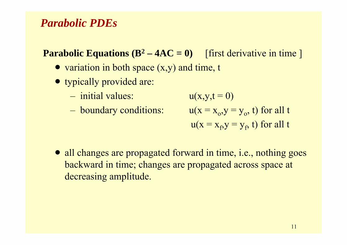
Parabolic Equations (B2 – 4AC = 0) [first derivative in time ]• variation in both space (x,y) and time, t• typically provided are:
– initial values: u(x,y,t = 0) – boundary conditions: u(x = xo,y = yo, t) for all t
u(x = xf,y = yf, t) for all t
• all changes are propagated forward in time, i.e., nothing goes backward in time; changes are propagated across space at decreasing amplitude.
12
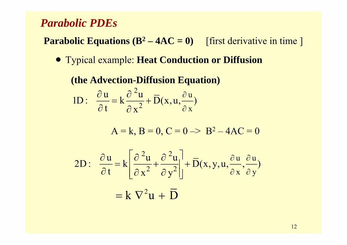
Parabolic PDEs Parabolic Equations (B2 – 4AC = 0) [first derivative in time ]
• Typical example: Heat Conduction or Diffusion
(the Advection-Diffusion Equation)2
2u
x
u u1D : k D(x,u, )t x
∂
∂
∂ ∂= +
∂ ∂
2 2
2 2u u
x y
u u u2D : k D(x, y,u, , )t x y
∂ ∂
∂ ∂
⎡ ⎤∂ ∂ ∂= + +⎢ ⎥∂ ∂ ∂⎢ ⎥⎣ ⎦
A = k, B = 0, C = 0 –> B2 – 4AC = 0
2k u D= ∇ +
13
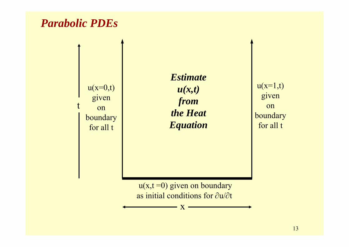
Parabolic PDEs
Estimateu(x,t)from
the HeatEquation
u(x=1,t)given
onboundaryfor all t
u(x,t =0) given on boundaryas initial conditions for ∂u/∂t
t
x
u(x=0,t)given
onboundaryfor all t
14
Parabolic PDEs
x=L
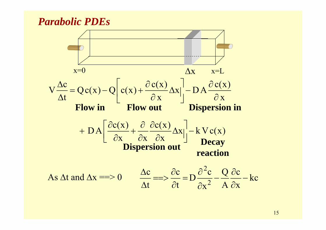
• An elongated reactor with a single entry and exit point and a uniform cross-section of area A.
• A mass balance is developed for a finite segment Δxalong the tank's longitudinal axis in order to derive a differential equation for concentration (V = A Δx).
Δxx=0
c(x,t) = concentrationat time, t, and distance, x.
15
Parabolic PDEs
x=LΔxx=0
c c(x) c(x)V Qc(x) Q c(x) x DAt x x
⎡ ⎤Δ ∂ ∂= − + Δ −⎢ ⎥Δ ∂ ∂⎣ ⎦
Flow in Flow out Dispersion in
c(x) c(x)DA x k Vc(x)x x x
∂ ∂ ∂⎡ ⎤+ + Δ −⎢ ⎥∂ ∂ ∂⎣ ⎦Dispersion out Decay
reaction2
2c c c Q cD kct t A xx
Δ ∂ ∂ ∂==> = − −
Δ ∂ ∂∂As Δt and Δx ==> 0
16
Hyperbolic PDEs
Hyperbolic Equations (B2 – 4AC > 0) [2nd derivative in time ]
• variation in both space (x, y) and time, t
• requires:– initial values: u(x,y,t=0), ∂u/∂t (x,y,t = 0) "initial velocity"– boundary conditions: u(x = xo,y = yo, t) for all t
u(x = xf,y = yf, t) for all t
• all changes are propagated forward in time, i.e., nothing goes backward in time.
Based on approximating solution at a finite # of points, usuallyarranged in a regular grid.
• Finite Element (FE) Method (C&C Ch. 31)Based on approximating solution on an assemblage of simply shaped (triangular, quadrilateral) finite pieces or "elements" which together make up (perhaps complexly shaped) domain.
In this course, we concentrate on FD applied to elliptic and parabolic equations.
20
Finite Difference for Solving Elliptic PDE's
Solving Elliptic PDE's:• Solve all at once• Liebmann Method:
– Based on Boundary Conditions (BCs) and finite difference approximation to formulate system of equations
– Use Gauss-Seidel to solve the system 2 2
2 2y
0u u u uD(x, y,u, , )x x y
∂ ∂
∂ ∂
⎧⎪ ∂ ∂+ = ⎨−⎪ ∂ ∂⎩
Laplace Eq.Poisson Eq.
21
Finite Difference Methods for Solving Elliptic PDE's1. Discretize domain into grid of evenly spaced points2. For nodes where u is unknown:
w/ Δ x = Δ y = h, substitute into main equation
3. Using Boundary Conditions, write, n*m equations for u(xi=1:m, yj=1:n) or n*m unknowns.
4. Solve this banded system with an efficient scheme. Using Gauss-Seidel iteratively yields the Liebmann Method.
i 1, j i, j i 1, j 22
2 2
u 2u u
xO( x )
u
x ( )− +− +
ΔΔ
∂
∂= +
2 22
2 2 2i 1, j i 1, j i, j 1 i, j 1 i, ju u u u 4uu u
O(h )x y h
− + − ++ + + −∂ ∂
∂ ∂+ = +
i, j 1 i, j i, j 1 22
2 2
u 2u u
yO( y )
u
y ( )− +− +
ΔΔ
∂
∂= +
22
Elliptical PDEs
The Laplace Equation2 2
2 2y
u u 0x
∂ ∂
∂ ∂+ =
The Laplace molecule
i i+1i-1j-1
j+1
j
i 1, j i 1, j i, j 1 i, j 1 i, jT T T T 4T 0+ − + −+ + + − =If Δx = Δy then
The temperature distribution can be estimated by discretizingthe Laplace equation at 9 points and solving the system of linear equations.
i 1, j i 1, j i, j 1 i, j 1 i, jT T T T 4T 0+ − + −+ + + − =
Excel
24
Solution of Elliptic PDE's: Additional Factors • Primary (solve for first): u(x,y) = T(x,y) = temperature distribution • Secondary (solve for second):
heat flux:
obtain by employing:
x yT Tq k and q kx y
∂ ∂′ ′= − = −∂ ∂
i 1, j i 1, jT TTx 2 x
+ −−∂≈
∂ Δi, j 1 i, j 1T TT
y 2 y−+ −∂
≈∂ Δ
then obtain resultant flux and direction:2 2
n x yq q q= + y1x
x
qtan q 0
q− ⎛ ⎞
θ = >⎜ ⎟⎝ ⎠
y1x
x
qtan q 0
q− ⎛ ⎞
θ = + π <⎜ ⎟⎝ ⎠
(with θ in radians)
25
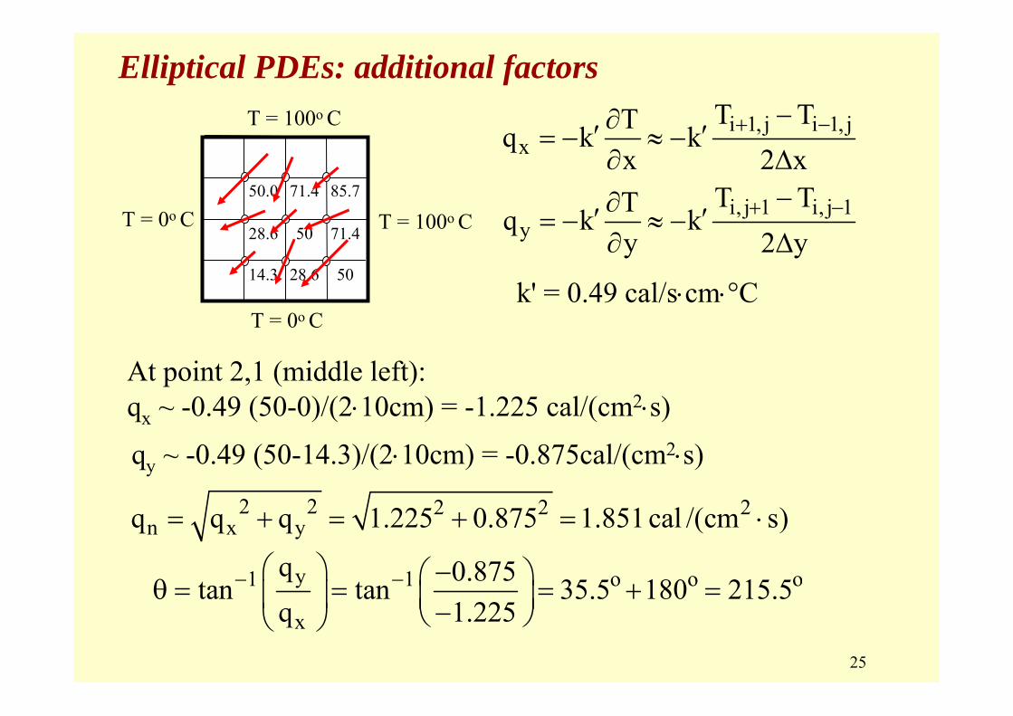
Elliptical PDEs: additional factorsi 1, j i 1, j
xT TTq k k
x 2 x+ −−∂′ ′= − ≈ −
∂ Δ
i, j 1 i, j 1y
T TTq k ky 2 y
+ −−∂′ ′= − ≈ −∂ Δ
k' = 0.49 cal/s⋅cm⋅°C
At point 2,1 (middle left):qx ~ -0.49 (50-0)/(2⋅10cm) = -1.225 cal/(cm2⋅s)
qy ~ -0.49 (50-14.3)/(2⋅10cm) = -0.875cal/(cm2⋅s)
T = 0o C
T = 100o C
T = 100o C
T = 0o C50.0 71.4 85.7
28.6 50 71.4
14.3 28.6 50
2 2 2 2 2n x yq q q 1.225 0.875 1.851 cal /(cm s)= + = + = ⋅
y1 1
x
q 0.875tan tan 35.5 180 215.5q 1.225
− −⎛ ⎞ −⎛ ⎞θ = = = + =⎜ ⎟ ⎜ ⎟−⎝ ⎠⎝ ⎠o o o
26
Solution of Elliptic PDE's: Additional Factors
Neumann Boundary Conditions (derivatives at edges)– employ phantom points outside of domain– use FD to obtain information at phantom point,
T1,j + T-1,j + T0,j+1 + T0,j-1 – 4T0,j = 0 [*]
If given then use
to obtain
Substituting [*]:
Irregular boundaries• use unevenly spaced molecules close to edge• use finer mesh
Tx
∂∂
1, j i 1, jT TTx 2 x
−−∂=
∂ Δ
1, j 1, jTT T 2 xx−
∂= − Δ
∂
1, j 0, j 1 0, j 1 0, jT2T 2 x T T 4T 0x + −
∂− Δ + + − =
∂
27
Elliptical PDEs: Derivative Boundary Conditions The Laplace molecule:
Insulated ==> ∂T/ ∂y = 0
T = 50o C
T = 100o C
T = 75o C1,1 1,2 1,3
2,1 2,2 2,3
3,1 3,2 3,3
i 1, j i 1, j i, j 1 i, j 1 i, jT T T T 4T 0+ − + −+ + + − =
5,1 3,1TT T 2 yy
∂= − Δ
∂
0
Derivative (Neumann) BC at (4,1):
3,1 5,1T - TT =y 2Δy
∂∂
4,2 4,0 3,1 4,12 2 4 0TT T T y Ty
∂− + − Δ − =
∂
Substitute into: 4,2 4,0 3,1 5,1 4,14 0T T T T T+ + + − =
To obtain:
28
Parabolic PDE's: Finite Difference Solution
Solution of Parabolic PDE's by FD Method• use B.C.'s and finite difference approximations to formulate
the model
• integrate I.C.'s forward through time
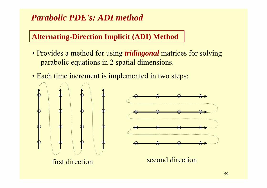
• for parabolic systems we will investigate: – explicit schemes & stability criteria – implicit schemes - Simple Implicit - Crank-Nicolson (CN) - Alternating Direction (A.D.I), 2D-space
29
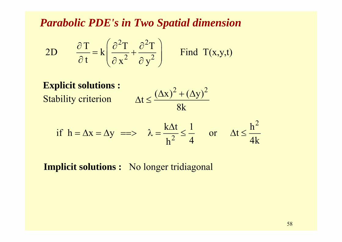
Parabolic PDE's: Heat Equation
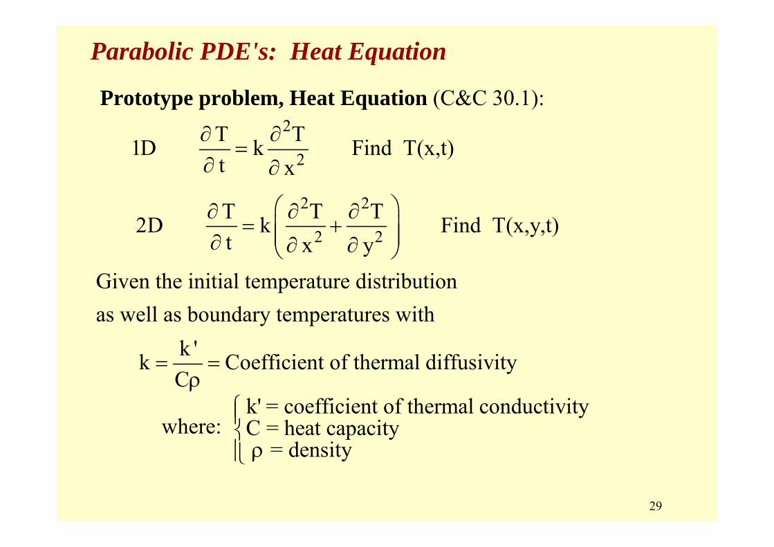
Prototype problem, Heat Equation (C&C 30.1):
Given the initial temperature distribution as well as boundary temperatures with
2
2T T1D k Find T(x,t)t x
∂ ∂=
∂ ∂2 2
2 2T T T2D k Find T(x,y,t)t x y
⎛ ⎞∂ ∂ ∂= +⎜ ⎟⎜ ⎟∂ ∂ ∂⎝ ⎠
k 'k Coefficient of thermal diffusivityC
= =ρ
k' = coefficient of thermal conductivityC = heat capacity = density
⎧⎪⎨
ρ⎪⎩where:
30
Parabolic PDE's: Finite Difference Solution
Solution of Parabolic PDE's by FD Method1. Discretize the domain into a grid of evenly spaces points
(nodes)2. Express the derivatives in terms of Finite Difference
Approximations of O(h2) and O(Δt) [or order O(Δt2)]
2
2T
x∂∂
3. Choose h = Δx = Δy, and Δt and use the I.C.'s and B.C.'s to solve the problem by systematically moving ahead in time.
Finite Differences
2
2T
y∂∂
Tt
∂∂
31
Parabolic PDE's: Finite Difference Solution
Time derivative:
• Explicit Schemes (C&C 30.2)
Express all future (t + Δt) values, T(x, t + Δt), in terms of current (t) and previous (t - Δt) information, which is known.
• Implicit Schemes (C&C 30.3 -- 30.4)
Express all future (t + Δt) values, T(x, t + Δt), in terms of other future (t + Δt), current (t), and sometimes previous (t - Δt) information.
32
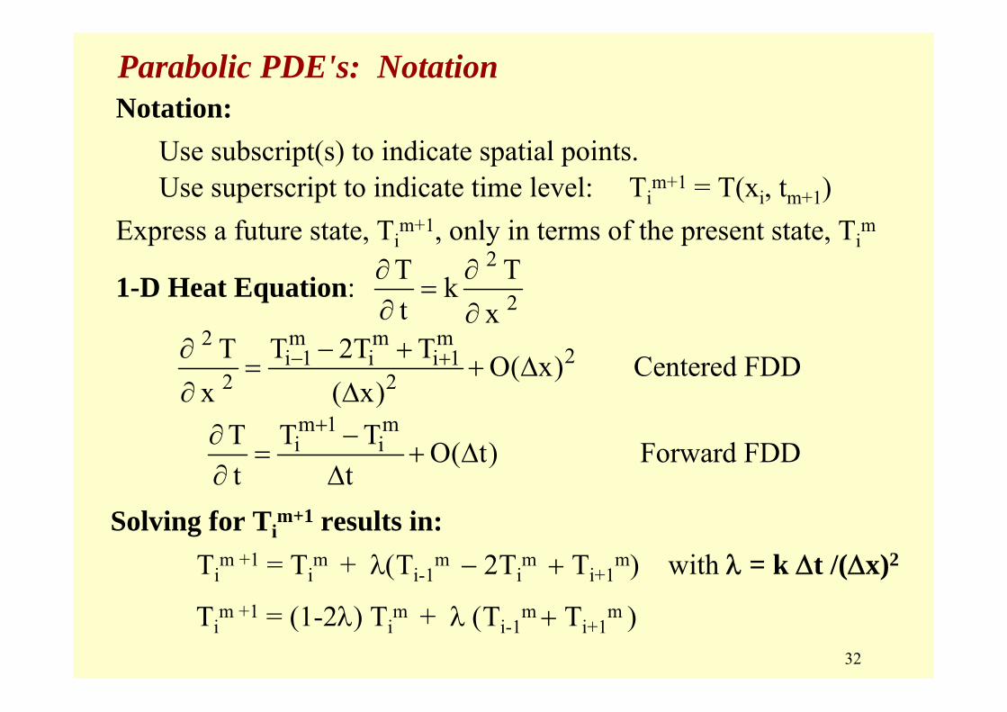
Parabolic PDE's: NotationNotation:
Use subscript(s) to indicate spatial points.Use superscript to indicate time level: Ti
m+1 = T(xi, tm+1)Express a future state, Ti
m+1, only in terms of the present state, Tim
1-D Heat Equation:2
2T Tkt x
∂ ∂=
∂ ∂2 m m m
2i 1 i i 12 2T T 2T T O( x) Centered FDD
x ( x)− +∂ − +
= + Δ∂ Δ
m 1 mi iT T T O( t) Forward FDD
t t
+∂ −= + Δ
∂ Δ
Solving for Tim+1 results in:
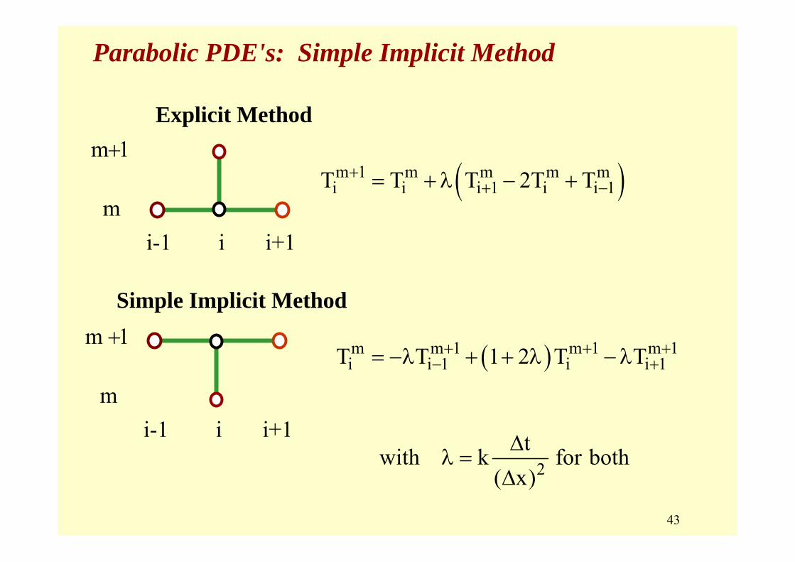
Tim +1 = Ti
m + λ(Ti-1m − 2Ti
m + Ti+1m) with λ = k Δt /(Δx)2
Tim +1 = (1-2λ) Ti
m + λ (Ti-1m + Ti+1
m )
33
Parabolic PDE's: Explicit method
t = 0
t = 1
t = 2
t = 3
t = 4
t = 5
t = 6
Initial temperature10 10 15 20 15 10 10 10
10
10
10
10
10
10
10
10
10
10
10
10
34
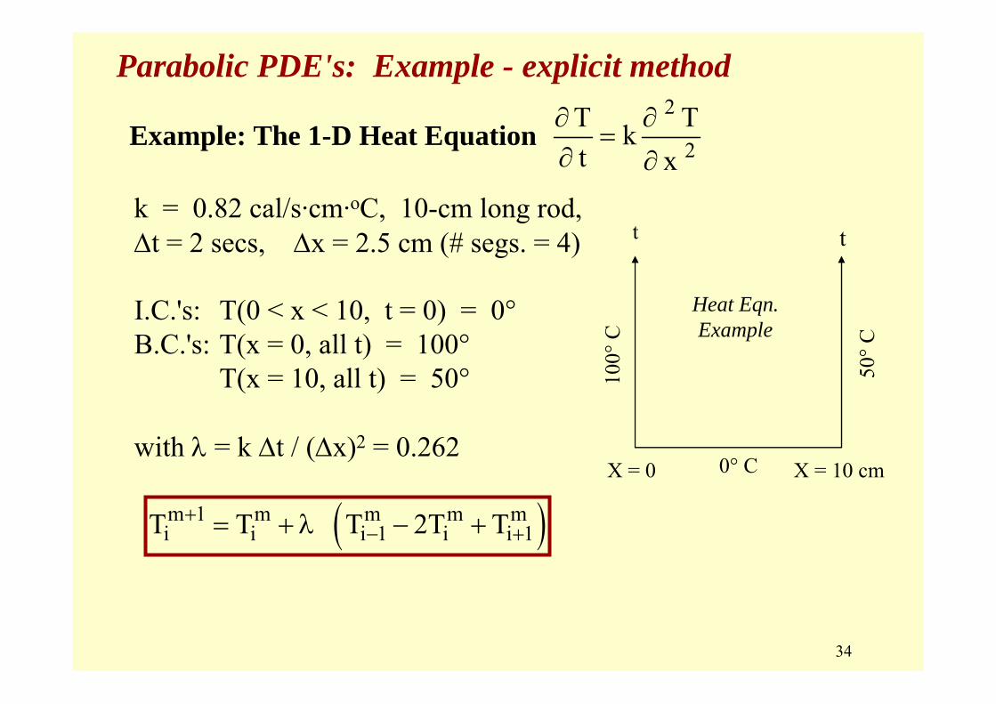
Parabolic PDE's: Example - explicit method
k = 0.82 cal/s·cm·oC, 10-cm long rod, Δt = 2 secs, Δx = 2.5 cm (# segs. = 4)
I.C.'s: T(0 < x < 10, t = 0) = 0°B.C.'s: T(x = 0, all t) = 100°
T(x = 10, all t) = 50°
with λ = k Δt / (Δx)2 = 0.262
2
2T Tkt x
∂ ∂=
∂ ∂Example: The 1-D Heat Equation
( )m 1 m m m mi i i 1 i i 1T T T 2T T+
− += + λ − +
Heat Eqn.Example
0° C
tt
100°
C
50°C
X = 0 X = 10 cm
35
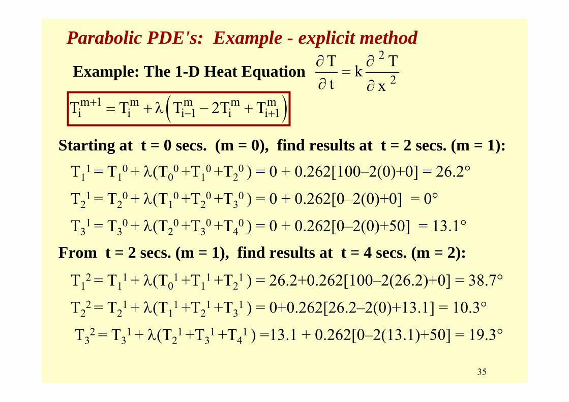
Parabolic PDE's: Example - explicit method
Starting at t = 0 secs. (m = 0), find results at t = 2 secs. (m = 1):T1
1 = T10 + λ(T0
0 +T10 +T2
0 ) = 0 + 0.262[100–2(0)+0] = 26.2°
T21 = T2
0 + λ(T10 +T2
0 +T30 ) = 0 + 0.262[0–2(0)+0] = 0°
T31 = T3
0 + λ(T20 +T3
0 +T40 ) = 0 + 0.262[0–2(0)+50] = 13.1°
From t = 2 secs. (m = 1), find results at t = 4 secs. (m = 2):
T12 = T1
1 + λ(T01 +T1
1 +T21 ) = 26.2+0.262[100–2(26.2)+0] = 38.7°
T22 = T2
1 + λ(T11 +T2
1 +T31 ) = 0+0.262[26.2–2(0)+13.1] = 10.3°
T32 = T3
1 + λ(T21 +T3
1 +T41 ) =13.1 + 0.262[0–2(13.1)+50] = 19.3°
2
2T Tkt x
∂ ∂=
∂ ∂Example: The 1-D Heat Equation
( )m 1 m m m mi i i 1 i i 1T T T 2T T+
− += + λ − +
36
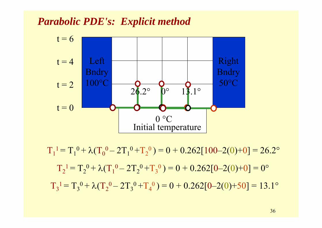
Parabolic PDE's: Explicit method
t = 0
t = 2
t = 4
t = 6
Initial temperature0 °C
RightBndry50°C
LeftBndry100°C
T11 = T1
0 + λ(T00 – 2T1
0 +T20 ) = 0 + 0.262[100–2(0)+0] = 26.2°
T21 = T2
0 + λ(T10 – 2T2
0 +T30 ) = 0 + 0.262[0–2(0)+0] = 0°
T31 = T3
0 + λ(T20 – 2T3
0 +T40 ) = 0 + 0.262[0–2(0)+50] = 13.1°
26.2° 0° 13.1°
37
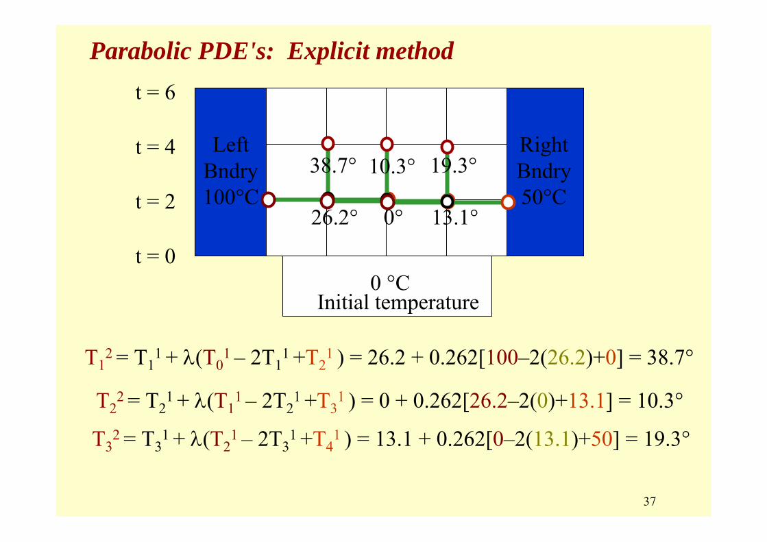
Parabolic PDE's: Explicit method
t = 0
t = 2
t = 4
t = 6
Initial temperature0 °C
RightBndry50°C
LeftBndry100°C
T12 = T1
1 + λ(T01 – 2T1
1 +T21 ) = 26.2 + 0.262[100–2(26.2)+0] = 38.7°
T22 = T2
1 + λ(T11 – 2T2
1 +T31 ) = 0 + 0.262[26.2–2(0)+13.1] = 10.3°
T32 = T3
1 + λ(T21 – 2T3
1 +T41 ) = 13.1 + 0.262[0–2(13.1)+50] = 19.3°
26.2° 0° 13.1°
38.7° 10.3° 19.3°
38
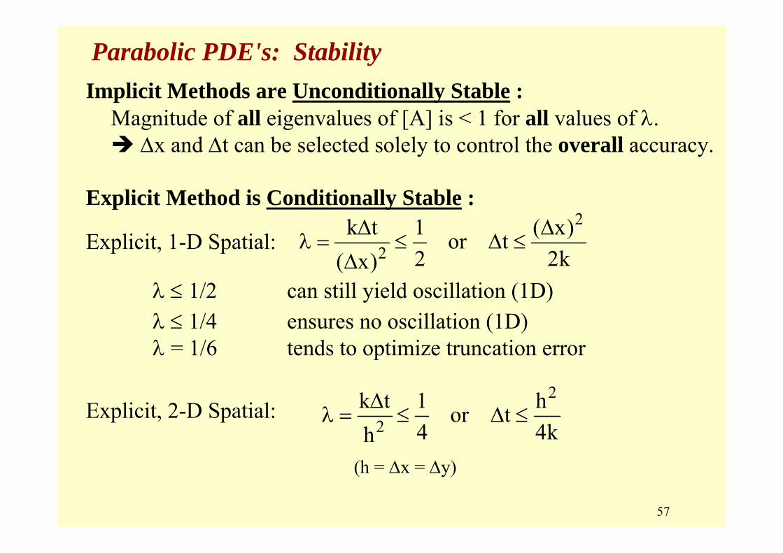
Parabolic PDE's: Stability
We will cover stability in more detail later, but we will show that:
The Explicit Method is Conditionally Stable :
For the 1-D spatial problem, the following is the stability condition:
λ ≤ 1/2 can still yield oscillation (1D)λ ≤ 1/4 ensures no oscillation (1D)λ = 1/6 tends to optimize truncation error
We will also see that the Implicit Methods are unconditionally stable.
2
2k t 1 ( x)or t
2 2k( x)Δ Δ
λ = ≤ Δ ≤Δ
Excel: Explicit
39
Parabolic PDE's: Explicit Schemes
Summary: Solution of Parabolic PDE's by Explicit Schemes
Advantages: very easy calculations, simply step ahead
Disadvantage: – low accuracy, O (Δt) accurate with respect to time
– subject to instability; must use "small" Δt'srequires many steps !!!
40
Parabolic PDE's: Implicit Schemes
Implicit Schemes for Parabolic PDEs
• Express Tim+1 terms of Tj
m+1, Tim, and possibly also Tj
m
(in which j = i – 1 and i+1 )
• Represents spatial and time domain. For each new time, write m (# of interior nodes) equations and simultaneously solve for m unknown values (banded system).
41
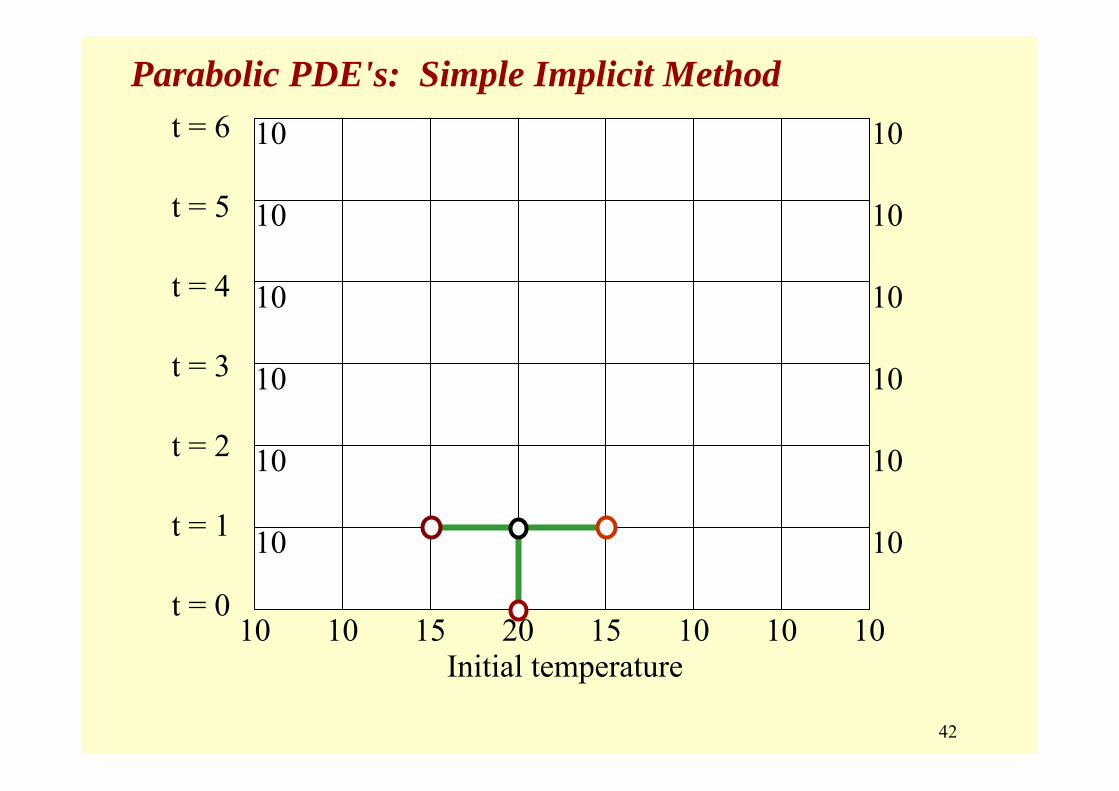
Simple Implicit Method. Substituting:
2 m 1 m 1 m 12i 1 i i 1
2 2T T 2T T O( x) Centered FDD
x ( x)
+ + +− +∂ − +
= + Δ∂ Δ
2
2T Tkt x
∂ ∂=
∂ ∂The 1-D Heat Equation:
results in: m 1 m 1 m 1 mi 1 i i 1 i 2
tT (1 2 )T T T with k( x)
+ + +− +
Δ−λ + + λ − λ = λ =
Δ1. Requires I.C.'s for case where m = 0: i.e., Ti
0 is given for all i.2. Requires B.C.'s to write expressions @ 1st and last interior
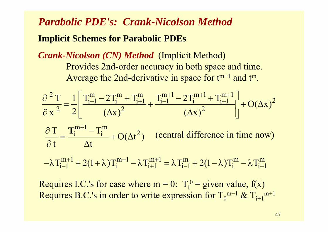
Parabolic PDE's: Crank-Nicolson MethodImplicit Schemes for Parabolic PDEs
Crank-Nicolson (CN) Method (Implicit Method)Provides 2nd-order accuracy in both space and time.Average the 2nd-derivative in space for tm+1 and tm.
2 m m m m 1 m 1 m 12i 1 i i 1 i 1 i i 1
2 2 2T 1 T 2T T T 2T T O( x)
2x ( x) ( x)
+ + +− + − +⎡ ⎤∂ − + − +
= + + Δ⎢ ⎥∂ Δ Δ⎢ ⎥⎣ ⎦
m 1 m2i iT T O( t )
t t
+∂ −= + Δ
∂ ΔT
m 1 m 1 m 1 m m mi 1 i i 1 i 1 i i 1T 2(1 )T T T 2(1 )T T+ + +− + − +−λ + + λ − λ = λ + − λ − λ
Requires I.C.'s for case where m = 0: Ti0 = given value, f(x)
Requires B.C.'s in order to write expression for T0m+1 & Ti+1
m+1
(central difference in time now)
48
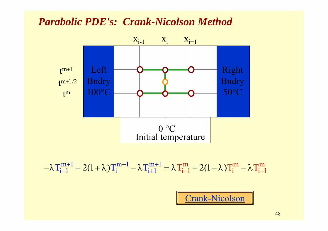
Parabolic PDE's: Crank-Nicolson Method
tm
tm+1
Initial temperature0 °C
RightBndry50°C
LeftBndry100°C
tm+1/2
xi-1 xi xi+1
m 1 m 1 m 1i 1 i i 1
m m mi 1 i i 12(1 ) 2(1 TT )TT T T+− +
+ +− +−λ + + λ − λ = λ + − λ − λ
Crank-Nicolson
49
Parabolic PDE's: Implicit Schemes
Summary: Solution of Parabolic PDE's by Implicit Schemes
Advantages:• Unconditionally stable. • Δt choice governed by overall accuracy.
[Error for CN is O(Δt2) ]• May be able to take larger Δt fewer steps
Disadvantages:• More difficult calculations,
especially for 2D and 3D spatially• For 1D spatially, effort ≈ same as explicit
because system is tridiagonal.
50
Stability Analysis of Numerical Solution to Heat Eq.
To find the form of the solutions, try:
Consider the classical solution of the Heat Equation:2
2T Tkt x
∂ ∂=
∂ ∂
atT(x, t) e sin( x)−= ω
Substituting this into the Heat Equation yields:- a T(x,t) = - k ω2 T(x,t)
OR a = k ω2
2k tT(x, t) e sin( x)− ω⇒ = ω
Each sin component of the initial temperature distribution decays as
exp{- k ω2 t)
51
Stability Analysis
with zero boundary conditions
First step can be written: {T1} = [A] {T0} w/ {T0} = initial conditions
Second step as: {T2} = [A] {T1} = [A]2{T0}
and mth step as:{Tm } = [A] {Tm-1} = [A]m{T0}
(Here "m" is an exponent on [A])
{ }m m m m m T1 2 i nwith T T ,T , ,T , ,T⎢ ⎥= ⎣ ⎦L L
Consider FD schemes as advancing one step with a "transition equation":
{Tm+1} = [A] {Tm} with [A] a function of λ = k Δt / (Δx)2
52
Stability Analysis
{Tm } = [A]m{T0}
• For the influence of the initial conditions and any rounding errors in the IC (or rounding or truncation errors introduced in the transition process) to decay with time, it must be the case that || A || < 1.0
• If || A || > 1.0, some eigenvectors of the matrix [A] can grow without bound generating ridiculous results. In such cases the method is said to be unstable.
• Taking r = || A || = || A ||2 = maximum eigenvalue of [A] for symmetric A (the "spectral norm"), the maximum eigenvalue describes the stability of the method.
53
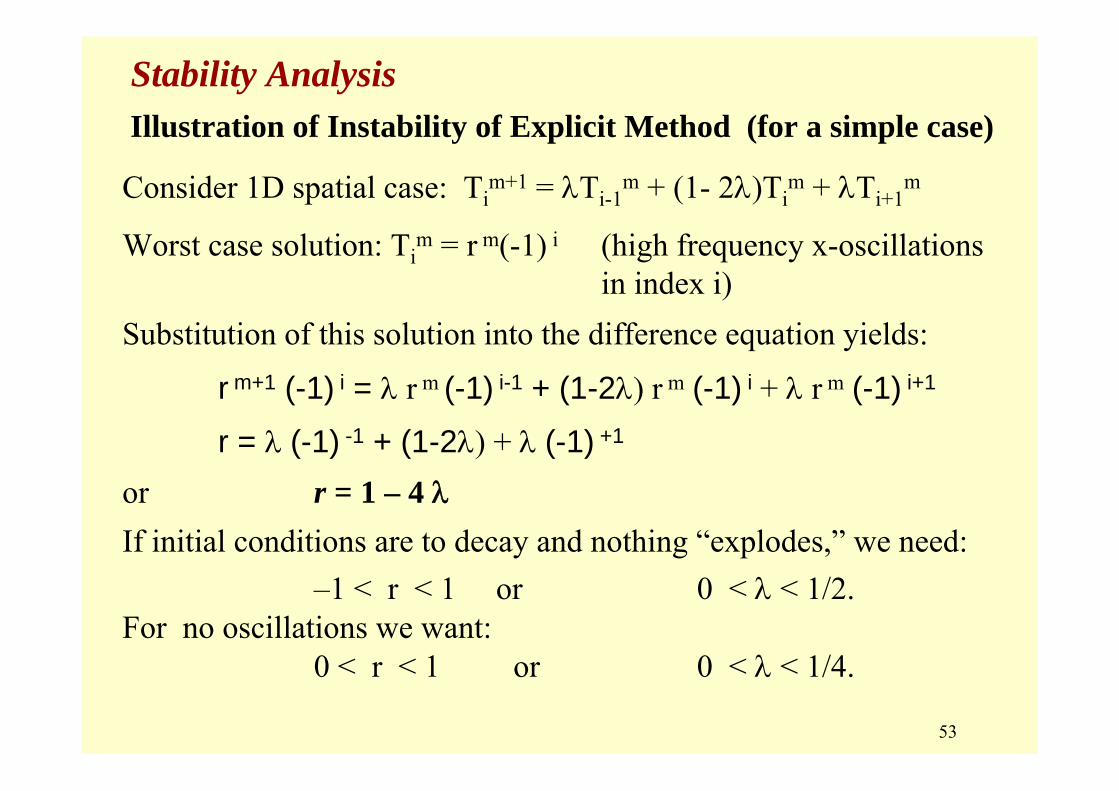
Stability AnalysisIllustration of Instability of Explicit Method (for a simple case)
Consider 1D spatial case: Tim+1 = λTi-1
m + (1- 2λ)Tim + λTi+1
m
Worst case solution: Tim = r m(-1) i (high frequency x-oscillations
in index i) Substitution of this solution into the difference equation yields:
r m+1 (-1) i = λ r m (-1) i-1 + (1-2λ) r m (-1) i + λ r m (-1) i+1
r = λ (-1) -1 + (1-2λ) + λ (-1) +1
or r = 1 – 4 λIf initial conditions are to decay and nothing “explodes,” we need:
–1 < r < 1 or 0 < λ < 1/2. For no oscillations we want:
0 < r < 1 or 0 < λ < 1/4.
54
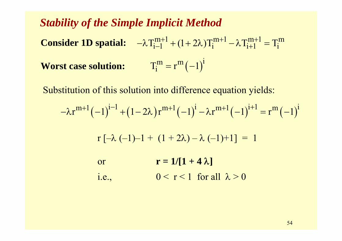
Stability of the Simple Implicit Method
Consider 1D spatial:
Worst case solution:
m 1 m 1 m 1 mi 1 i i 1 iT (1 2 )T T T+ + +− +−λ + + λ − λ =
( )im miT r 1= −
Substitution of this solution into difference equation yields:
( ) ( ) ( ) ( ) ( )i 1 i i 1 im 1 m 1 m 1 mr 1 1 2 r 1 r 1 r 1− ++ + +−λ − + − λ − − λ − = −
r [–λ (–1)–1 + (1 + 2λ) – λ (–1)+1] = 1
or r = 1/[1 + 4 λ]i.e., 0 < r < 1 for all λ > 0
55
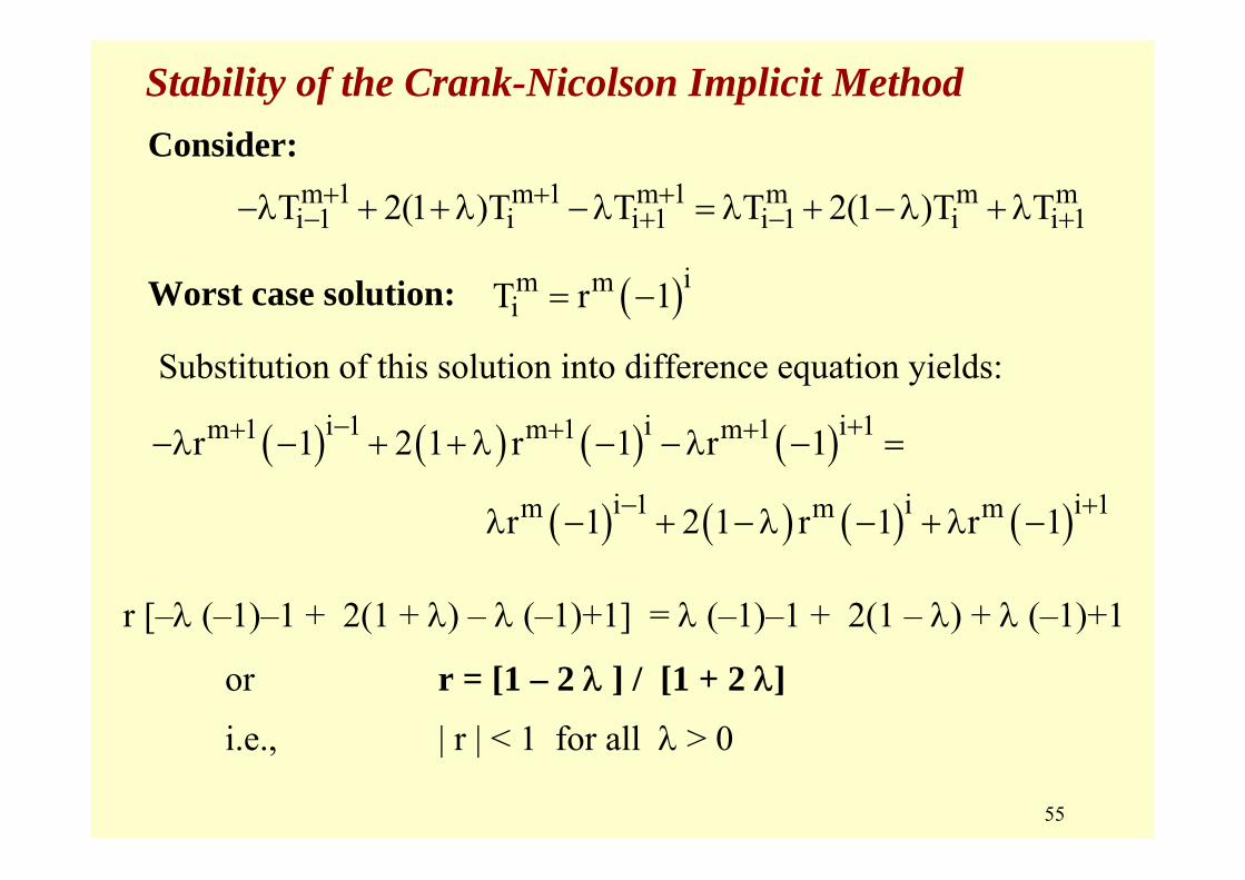
Stability of the Crank-Nicolson Implicit MethodConsider:
Worst case solution:
Substitution of this solution into difference equation yields:
m 1 m 1 m 1 m m mi 1 i i 1 i 1 i i 1T 2(1 )T T T 2(1 )T T+ + +− + − +−λ + + λ − λ = λ + − λ + λ
( )im miT r 1= −
( ) ( ) ( ) ( )i 1 i i 1m 1 m 1 m 1r 1 2 1 r 1 r 1− ++ + +−λ − + + λ − − λ − =
( ) ( ) ( ) ( )i 1 i i 1m m mr 1 2 1 r 1 r 1− +λ − + − λ − + λ −