Master’s Thesis Solution of the Navier-Stokes Equation using the Method of Characteristic Curves Student Jos´ e David Villegas Jim´ enez Responsible professor Manuel Julio Garc´ ıa Ruiz Department of Mechanical Engineering Universidad EAFIT Medell´ ın January, 2014
Transcript
Master’s Thesis
Solution of the Navier-Stokes Equation using the
Method of Characteristic Curves
Student
Jose David Villegas Jimenez
Responsible professor
Manuel Julio Garcıa Ruiz
Department of Mechanical Engineering
Universidad EAFIT
Medellın
January, 2014
Abstract
This project deals about the solution of the Navier Stokes Equations by the Method of
Characteristics. This method is used to eliminate the convective part of equations of
the convection-diffusion type, conducting the material derivative in a Lagrangian manner
along the characteristic curves of each node in a fixed grid. Following this approach, the
method is able to solve the incompressible Navier Stokes Equations with the advantage
of using large timesteps. In the present case, the solution of the well known Lid Driven
Cavity Flow problem is obtained for several Reynolds numbers, showing good agreement
when compared to solutions obtained by other methods.
Keywords: Characteristic curves, Finite Element Method, Lagrange-Galerkin Method,
projection schemes, Fractional Step Methods and recently, a group of meshless methods
which are becoming popular because complex geometries as well as large deformations,
nonlinearities, crack simulations can be treated with ease. The problem with some of
these methods is the definition of boundary conditions. These kinds of methods include,
the Element-Free Galerkin Method (EFG) Belytschko et al. (1994), Isoparametric Finite
Point Method Wang and Takao (2004), Meshless local Petrov-Galerkin (MLPG) Atluri
and Zhu (1998), Smooth Particle Hydrodynamics (SPH)Gingold and Monaghan (1977),
Moving Particle Semi-Implicit Method (MPS)Koshizuka et al. (1998), among others.
1
2 CONTENTS
The characteristic based method is followed according to the work done by Zienkiewicz
et al. (2005), Zienkiewicz et al. (1999) and contributions of (Nithiarasu (2003), Nithiarasu
(2002)). This method is based on a splitting technique proposed by Chorin (1968), re-
lated to Fractional Step Methods in which velocity and pressure operators are decoupled.
The use of an artificial compressibility method is convenient to overcome computational
difficulties when treating the conservation equation Nithiarasu (2003).
The formulation of a Lagrange-Galerkin Method, first introduced by Benque et al.
(1980) involving Characteristic curves is covered in the second part of this work. This
method is proved to be efficient for convection dominated problems as illustrated by
Boukir et al. (1997), Achdou and Guermond (2000), Pironneau (1982) and is stated
as a mixture of a traditional Galerkin Method for spatial variables with a Lagrangian
formulation for time. This method is set as a mixed formulation in which, a penalty
method to solve the system of equations introduces a small perturbation coefficient in the
conservation equation, in order to be able to solve the matricial system, achieved after
proposing a variational formulation for the problem.
This work provides another approach to the solution of Navier Stokes Equations,
presenting the equations in discrete form in a simple manner, treating the temporal term
of the equation with a finite different scheme and in contrast to the unstructured triangular
grid formulations found in the literature, the use of a structured grid of square elements.
This document is organized as follows. In chapter 1 generalities of the Navier-Stokes
Equation (section 1.1) and the concept of characteristic curves (section 1.2) are explained.
In chapter 2 some features of the Characteristic Based Method (CBS) are reviewed. The
Lagrange-Galerkin or characteristic curve method is introduced in chapter 3, and finally
an example of the lid driven cavity flow is solved by the Lagrange-Galerkin procedure and
discussed on sections 3.2 and 3.3 respectively.
Chapter 1
Preliminary Concepts
1.1 Navier Stokes Equation
The Navier Stokes equations describe the behavior of viscous fluids and are derived from
the conservation laws, namely, the Newton’s law of motion, the continuity equation and
the energy equation. These coupled set of equations are Hyperbolic Partial Differential
Equations of first or second order that describe time-dependent convection dominated
problems. The law of momentum conservation states that the rate of change of momentum
of a particle equals the sum of external forces applied to it, therefore it is important to
mention that the deduction of the Navier Stokes equation is based on this law. The
left hand side of equation 1.1 shows the rate of change of momentum , while the right
hand side shows the sum of body forces, acting throughout the volume of a body (i.e
gravitational forces), and contact forces, interacting with the fluid element throughout its
surface (i.e viscous forces).
ρ
(∂u
∂t+ u · ∇u
)︸ ︷︷ ︸Change in momentum
= div(σ)︸ ︷︷ ︸Surface force
+ ρb︸︷︷︸Body force
. (1.1)
In order to achieve the Navier Stokes set of equations, a constitutive relation for
the stress (σ) must be defined and incorporated; for a Newtonian incompressible fluid
(div(u) = 0) we have,
σ = 2µD − pI.
3
4 Preliminary Concepts
where σσσ is the stress, µµµ is the dynamic viscosity, D = 12
(∇u +∇uT
)is the strain rate
or deformation tensor, p is the pressure and I is the identity matrix.
The set of equations is now complete:
ρ
(∂u
∂t+ u · ∇u
)= µ∇2u+ (µ+ λ)∇ (div(u))−∇p+ ρb
∇ · u = 0. (1.2)
For the case of incompressible fluids, density (ρ) is constant and the second term of
1.2 vanishes.
ρ
∂u
∂t︸︷︷︸Local accel.
+ u · ∇u︸ ︷︷ ︸Convective accel.
︸ ︷︷ ︸
Material derivative
= µ∇2u︸ ︷︷ ︸V iscous term
− ∇p︸︷︷︸Pressure term
+ ρb︸︷︷︸Body force term
∇ · u = 0. (1.3)
In order to complete the Navier Stokes problem, the set of equations must be subjected
to initial and boundary conditions. Initial conditions refer to the definition of initial
values for the velocity and pressure fields, while boundary conditions are imposed on the
boundary ΓΓΓ = Γ1 ∪ Γ2 ∪ Γ3 of an open fluid domain denoted by ΩΩΩ.
Figure 1.1: Open fluid domain Ω with its boundary Γ = Γ1 ∪ Γ2 ∪ Γ3
Boundary conditions are of three types as follows,
Dirichlet u = g on Γ1
Neumann h = [σ]n on Γ2
Robin [σ]n = α(u− uref ) on Γ3 (1.4)
1.2 The Concept of Characteristic Curve 5
where g is a defined function or constant, h is the traction or surface force,α is a
constant and uref is a reference velocity.
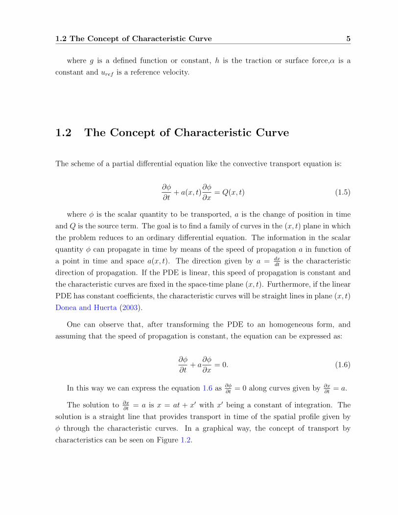
1.2 The Concept of Characteristic Curve
The scheme of a partial differential equation like the convective transport equation is:
∂φ
∂t+ a(x, t)
∂φ
∂x= Q(x, t) (1.5)
where φ is the scalar quantity to be transported, a is the change of position in time
and Q is the source term. The goal is to find a family of curves in the (x, t) plane in which
the problem reduces to an ordinary differential equation. The information in the scalar
quantity φ can propagate in time by means of the speed of propagation a in function of
a point in time and space a(x, t). The direction given by a = dxdt
is the characteristic
direction of propagation. If the PDE is linear, this speed of propagation is constant and
the characteristic curves are fixed in the space-time plane (x, t). Furthermore, if the linear
PDE has constant coefficients, the characteristic curves will be straight lines in plane (x, t)
Donea and Huerta (2003).
One can observe that, after transforming the PDE to an homogeneous form, and
assuming that the speed of propagation is constant, the equation can be expressed as:
∂φ
∂t+ a
∂φ
∂x= 0. (1.6)
In this way we can express the equation 1.6 as ∂φ∂t
= 0 along curves given by ∂x∂t
= a.
The solution to ∂x∂t
= a is x = at + x′ with x′ being a constant of integration. The
solution is a straight line that provides transport in time of the spatial profile given by
φ through the characteristic curves. In a graphical way, the concept of transport by
characteristics can be seen on Figure 1.2.
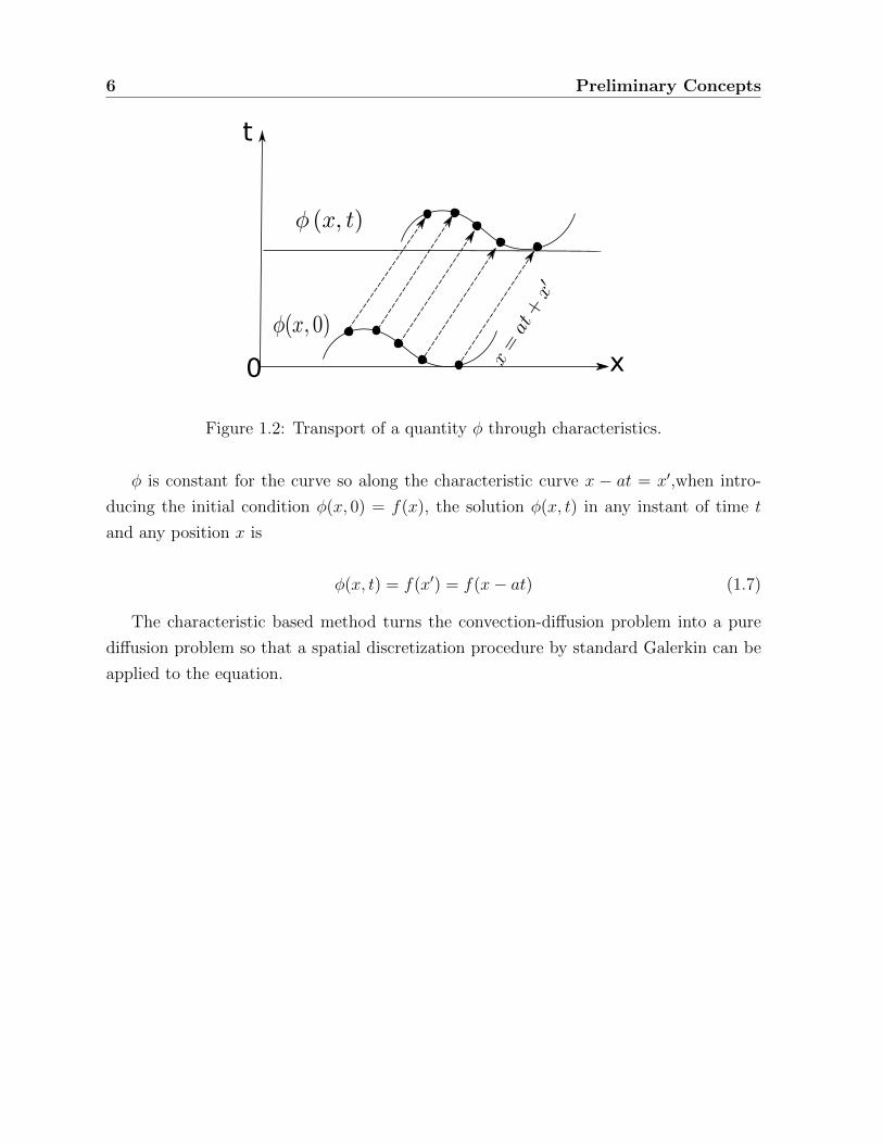
6 Preliminary Concepts
x
t
0
Figure 1.2: Transport of a quantity φ through characteristics.
φ is constant for the curve so along the characteristic curve x − at = x′,when intro-
ducing the initial condition φ(x, 0) = f(x), the solution φ(x, t) in any instant of time t
and any position x is
φ(x, t) = f(x′) = f(x− at) (1.7)
The characteristic based method turns the convection-diffusion problem into a pure
diffusion problem so that a spatial discretization procedure by standard Galerkin can be
applied to the equation.
Chapter 2
Characteristic-based Split Method
(CBS)
The characteristic based method is used to find a solution of fluid dynamics equations for
any condition of the flow (compressible or incompressible) by means of a standard Galerkin
procedure on characteristic curves. The method called CBS by Zienkiewicz et al. (2005)
is able to eliminate the convective part of the equation of momentum conservation after
setting it out in a Lagrangian fashion. Further discretization of the convection-diffusion
equation will provide ideas for the treatment of Navier Stokes Equations.
2.1 Galerkin Based Characteristic Method
2.1.1 Convection-diffusion equation
After laying out the concept of characteristic curves, the solution of mass and momentum
equations (Navier-Stokes Equations) for velocity and pressure variables (u and p) is con-
sidered. The main idea is to achieve the solution of these equations following a Galerkin
procedure based on characteristics.
In this method, the convection-diffusion equation can be split in two parts, a convective
term and a diffusive term that are discretized in a separate style. We have then the
7
8 Characteristic-based Split Method (CBS)
convection-diffusion equation:
∂φ
∂t︸︷︷︸T ime term
+∂
∂xj(ujφ)︸ ︷︷ ︸
Convective term
− ∂
∂xi
(k∂φ
∂xi
)︸ ︷︷ ︸Diffusive term
+ Q︸︷︷︸Source term
= 0. (2.1)
The split is done according to (2.2) as
φ = φ∗ + φ∗∗ (2.2)
∂φ∗
∂t+ U
∂φ
∂x= 0
∂φ∗∗
∂t− ∂
∂x
(k∂φ
∂x
)+Q = 0. (2.3)
This split will be explained subsequently while discretizing the Navier Stokes Equa-
tions.
The idea of the characteristic based Galerkin method is to perform a time discretiza-
tion for the convection-diffusion equation in moving coordinates (characteristics). This
operation is done having in mind the elimination of the convective term and the use of a
standard Galerkin procedure for the spatial discretization of remaining terms.
Taking the convection-diffusion equation on moving coordinates x′:
∂φ(x′)
∂t︸ ︷︷ ︸T ime term
− ∂
∂x′i
(k∂φ
∂x′i
)︸ ︷︷ ︸Diffusive term
+ Q(x′)︸ ︷︷ ︸Source term
= 0. (2.4)
Discretization of the time term is performed by setting out an approximation of the
scalar quantity φ in two different states of time: present time (t = tn), and a later time
(t = tn+1). The approximation uses an operator L acting on the scalar quantity to be
transported on both time moments
∂φ
∂t= L(φ) (2.5)
∂φ
∂t≈φn+1 − φn
∆t= L(φ)
L(φn+1) Unknown (Implicit)
L(φn) Known (Explicit)(2.6)
The approximation of the spatial, diffusive and source terms can be done following
an implicit, semi-implicit or explicit scheme according to a parameter θ. The most used
2.1 Galerkin Based Characteristic Method 9
scheme is the semi-implicit(θ = 1
2
), often called Crank-Nicolson.
∂φ
∂t≈φn+1 − φn
∆t= θL(φn+1) + (1− θ)L(φn)
θ = 1 Implicit
θ = 12
Semi− implicit
θ = 0 Explicit
(2.7)
After the discretization process, an expression for the explicit convection-diffusion
equation is achieved,
φn+1 − φn = −∆t
[∂(Ujφ)
∂xj− ∂
∂xi
(k∂φ
∂xi
)+Q
]t=n
+
∆t2
2Uk
∂
∂xk
[(∂(Ujφ)
∂xj
)− ∂
∂xi
(k∂φ
∂xi
)+Q
]t=n
.
(2.8)
The advantage of using this equation is that it is written in conservative form, and is
explicit because it is evaluated at present time t = n.
2.1.2 Navier Stokes equation
In a similar fashion we can discretize the Navier–Stokes equations in time:
In the Navier Stokes Equations the quantity to be transported is the velocity φ =
ρui = Ui. The convective term becomes the convective acceleration and the diffusive
term is the divergence of the strain forces, which are in fact given by the gradient of the
velocity. Finally, the pressure term is treated as a source term as well as the body forces.
Hence, the Navier–Stokes equations represent the convection-diffusion of momentum per
unit mass
∂Ui∂t
+∂
∂xj(ujUi)−
∂τij∂xj
+∂p
∂xi− ρgi︸ ︷︷ ︸
Source term
= 0. (2.9)
The scalar quantity is given by Ui = ρui.
After discretization of the Navier–Stokes Equations followed by a Crank Nicholson
10 Characteristic-based Split Method (CBS)
scheme with θ = 12, we can obtain an explicit equation for a time instant t = n
∆Ui =−∆t
[∂
∂xj(ujUi)−
∂τij∂xi
+∂p
∂xi− ρgi
]n+
∆t2
2uk
∂
∂xk
[∂
∂xj(ujUi)−
∂τij∂xi
+∂p
∂xi− ρgi
]n.
(2.10)
The following step is to split the equation isolating the pressure terms and expressing the
change of velocity ∆Ui as the sum of two auxiliary variables ∆U∗i and ∆U∗∗i , according
to (2.11):
∆Ui = ∆t
[− ∂
∂xj(ujUi) +
∂τij∂xi
+ ρgi
]n−∆t
∂pn+θ2
∂xi
+∆t2
2uk
∂
∂xk
[∂
∂xj(ujUi)−
∂τij∂xi− ρgi
]n︸ ︷︷ ︸
∆U∗i
+∆t2
2uk
∂
∂xk
(∂pn+θ2
∂xi
)︸ ︷︷ ︸
∆U∗∗i
(2.11)
∆Ui = ∆U∗i + ∆U∗∗i . (2.12)
The pressure terms that were separated are stored in the auxiliary variable ∆U∗∗i ,
whereas remaining terms are stored in ∆U∗i . Higher order terms in the stress tensor are
neglected
∆U∗i = ∆t
[−∂(ujUi)
∂xj+∂τij∂xj
+ ρgi +∆t
2uk
∂
∂xk
(∂(ujUi)
∂xj− ρgi
)]n. (2.13)
∆U∗∗i = −∆t∂pn+θ2
∂xi+
∆t2
2uk
∂2pn
∂xk∂xi(2.14)
As there is an additional unknown in the system (the pressure) we need an additional
equation to find it. Regarding the mass conservation equation, it is necessary to take
it to an alternate form in order to discretize and solve it. Depending on the problem
conditions, i.e. a compressible problem, density can be interpolated. Let us use the speed
of sound denoted by c
2.1 Galerkin Based Characteristic Method 11
∂ρ
∂t+ div(ρu) = 0 (2.15)
and also1
c2
∂p
∂t= − div(ρu).
Therefore,∂ρ
∂t=
1
c2
∂p
∂t= − div(ρu) = −∂Ui
∂xi
Using a θ time approximation for the conservation equation
∆ρ
∆t=
(1
c2
)n∆p
∆t= −∂U
n+θ1i
∂xi, (2.16)
which can be expanded as(1
c2
)n∆p
∆t= −∂U
n+θ1i
∂xi= −
[∂Un
i
∂xi+ θ1
∂∆Ui∂xi
],
and splitting the velocity(1
c2
)n∆p
∆t= −
[∂Un
i
∂xi+ θ1
∂
∂xi(∆U∗i + ∆U∗∗i )
].
Using the equation for ∆U∗∗ (2.14)(1
c2
)n∆p
∆t= −
[∂Un
i
∂xi+ θ1
∂
∂xi
(∆U∗i +−∆t
∂pn+θ2
∂xi+
∆t2
2uk
∂2pn
∂xk∂xi
)].
Since the last term is of superior order, and expanding pn+θ2 = pn + θ2∆p,(1
c2
)n∆p
∆t= −
[∂Un
i
∂xi+ θ1
∂∆U∗i∂xi
+−∆tθ1∂
∂xi
(∂pn
∂xi+ θ2
∂∆p
∂xi
)]. (2.17)
The method finishes with the solution of the equations after a Galerkin procedure in
the following order:
1. Solve (2.13) to obtain ∆U∗i .
2. Solve (2.17) to obtain ∆p o ∆ρ.
12 Characteristic-based Split Method (CBS)
3. Solve (2.14) to establish values for velocity and pressure in tn+1.
If a compressible problem is treated, it becomes necessary to get the energy equation
solved.
2.2 Spatial discretization
2.2.1 Step 1
The time discretization process through the characteristic based Galerkin method provides
a solution procedure for which it is necessary to follow a spatial discretization of equations
using the standard Galerkin method in order to achieve a matricial system of equations.
The process starts with the variational treatment of equation 2.13 to be taken to its weak
form
∆U∗i = ∆t
[−∂(ujUi)
∂xj+∂τij∂xj
+ ρgi +∆t
2uk
∂
∂xk
(∂(ujUi)
∂xj− ρgi
)]n.
The equation can be expressed in vector notation as follows:
∆U ∗ = ∆t
[− div(u⊗U) + div(τ ) + b+
∆t
2[∇(div (u⊗U)− b)]u
]n(2.18)
Both sides of the equation are multiplied by an arbitrary function v, with the same
features and from the same space of u, and integrated over the whole domain of analysis
Ω. ∫Ω
∆U ∗ · v︸ ︷︷ ︸1
=
∫Ω
∆t
[− div(u⊗U)︸ ︷︷ ︸
2
+ div(τ )︸ ︷︷ ︸3
+ b︸︷︷︸4
+∆t
2
∇(div(u⊗U)− b)u︸ ︷︷ ︸5
n · v. (2.19)
The suitable form of discretizing the equation is taking each one of the terms separately
to the matricial form. Before starting the discretization of each term, it is necessary to
define the way the functions U and v are approximated. Functions are approximated
multiplying the base functions of the element with the variables at each node . The initial
velocity vector u will be interpolated in the same manner as the unknown velocity vector
2.2 Spatial discretization 13
U
Ui(x) =∑b
U biN
b(x) vi(x) =∑a
vaiNa(x) (2.20)
with a, b: node number and i: dimension index. u can be expressed in vector notation as
u =∑i b
ubiNb(x)ei (2.21)
which we will call index approximation of the vector field. And the compact notation
which requires to be written as
N = [N1, N2, . . . , Nn], ui =
u1i...
uni
,where n is the number of nodes. Then
ui = Nui and u = Nu
where u is the matrix, form by the nodal values in the 1, 2 and 3 directions
u = N [u1u2u3] = N
u1
1 u12 u1
3...
......
un1 un2 un3
As said before, we must start the process with the first term.
1.∫
Ω∆U∗i · vi ∫
Ω
∆U∗i · vi ≈∫
Ω
N b∆U b∗i N
avia = vai ∆U
b∗i
∫Ω
NaN b
The product of both basis function vectors gives the mass matrix of the equation,
Mab
vai Mab∆U b∗
i =⟨vi , M∆U
∗i
⟩.
14 Characteristic-based Split Method (CBS)
2.∫
Ωdiv(u⊗U) · v
Let us continue with the discretization of the second term denoted by 2 in (2.19):∫Ω
div(u⊗U) · v.
∫Ω
∂
∂xj(ujUi)vi ≈
∫Ω
∂
∂xj(ujU
biN
b)vaiNa
= vai Ubi
∫Ω
∇(uN b)Na︸ ︷︷ ︸Cab
= vai CabU b
i
=⟨vi , CU i
⟩.
3.∫
Ωdiv(τ ) · v
The third term is the divergence of the deviatoric stress tensor τ . We must begin
integrating by parts the inner product of the divergence tensor with the arbitrary
function v
∫Ω
∂τij∂xj
vi =
∫Ω
div(τ ) · v =
∫Ω
div(τ i)vi
where τ i = [τi1, τi2, τi3], is the ith row of the stress tensor. Using the divergence
theorem 1 ∫Ω
div(τ i)vi = −∫
Ω
〈τ i,∇vi〉+
∫Γ
〈τ ivi,n〉 .
1 Given F a vector function and g a scalar function, the divergence theorem stands∫Ω
div (F g) =
∫Ω
(div (F ) g + 〈F ,∇g〉
)=
∫Γ
〈F g, n〉 .
2.2 Spatial discretization 15
The same result can be obtained using index notation and integration by parts∫Ω
∂τij∂xj
vi = −∫
Ω
τij∂vi∂xj
+
∫Γ
τijvinj
= −∫
Ω
∇v : τ︸ ︷︷ ︸a
+
∫Γ
〈t,v〉︸ ︷︷ ︸b
where ti = τijnj is the traction on the surface
After integration we get two terms, the first one (a) is integrated over the domain
and contains a Frobenius inner product of matrices often called double dot product,
whereas the other (b) is simply evaluated at the boundary and contains the traction
or product between the stress tensor and a normal vector on the surface.
A : B =∑ij
AijBij
a. First, the term integrated over the domain is discretized:
For a Newtonian fluid the following relationship is true,
τ = 2µ
(ε− 1
3div(ε)I
)with ε =
1
2(∇u+∇uT ),
where µ is the dynamic viscosity, ε = ε(u) is the strain rate and I is the identity
matrix. It should be noted that ε and τ are linear functionals. That is, given
u and v in V a vector space of admissible velocities, and given α ∈ R, then
(i) ε(u+ v) = ε(u) + ε(v)
(ii) ε(αv) = αε(u).
The same holds for the divergence and grad operators
div(αu+ βv) = α div(u) + β div(v)
∇(αu+ βv) = α∇(u) + β∇(v).
Using the linearity of these operators we can rewrite the strain rate, the diver-
gence and the the stress in terms of the base, (2.21). For the strain rate we
16 Characteristic-based Split Method (CBS)
have
ε(u) = ε(ubiNbei) = ubiε(Nbei).
By definition,
ε(u)rs =1
2(ur,s + ur,s) ,
so in the same manner
ε(Nbei)rs =1
2((Nbei)r,s + (Nbei)r,s)
=1
2(Nb,sδir +Nb,rδis) .
Therefore,
ε(u)rs = ubiε(Nbei)rs =ubi2
(Nb,sδir +Nb,rδis) . (2.22)
In the divergence case
div(u) = u,kk,
therefore
div(ubiNbei) = ubi(Nbei),kk = ubiNb,kδik, (2.23)
and in the gradient case
∇(v) = vr,s,
therefore
∇(vajNaej) = (vajNaej)r,s = vajNa,sδjr. (2.24)
Merging (2.22), (2.23) (2.24), and using index notation
σ : ∇v = 2µ
(ε(u)− 1
3div(ε)I
): ∇v
= 2µ
(ε(u)rs −
1
3ukkδrs
)vr,s
= µubi
((Nb,sδir +Nb,rδis)−
2
3Nb,kδikδrs
)vaiNa,sδjr.
Now, this expresion must be integrated over the domain, so it can be expressed
2.2 Spatial discretization 17
in a compact form as ∫Ω
σ : ∇v = ubivaiK
abji , (2.25)
with
Kabij =
∫Ω
((Nb,sδir +Nb,rδis)−
2
3Nb,kδikδrs
)Na,sδjr. (2.26)
Combining two indexes in one yields
α = 2(a− 1) + j
β = 2(b− 1 + i).
We can rewrite the expression above in simple matrix notation as
〈v,Ku〉 .
b. The term integrated over the boundary Γ contains the traction and is dis-
cretized as follows:
∫Γ
t · v ≈∫
Γ
tiNavai
= vai
∫Γ
tiNa
= vai2
fai
where ∫Γ
tiNa =
2
fai (2.27)
in compact form, and combining subindices the last product can be interpreted
as a dot product. The final discrete expression for the term is∫Ω
div(τ ) · v → 〈v,Ku〉+
⟨v,
2
f
⟩(2.28)
4.∫
Ωb · v
The fourth term related to body forces, is discretized assuming constant density for
18 Characteristic-based Split Method (CBS)
the element
∫Ω
b · v ≈∫
Ω
ρgiNavai
= vai
∫Ω
ρgiNa
= vai1
fai
=
⟨v,
1
f
⟩where ∫
Ω
ρgiNa =
1
fai . (2.29)
5.∫
Ω∇(div(u⊗U)− b)u · v
The next term to discretize is the stabilizing term denoted by number 5. It should
be mentioned that this term has two components: a matrix and a vector. To ease
the process, we may take advantage of alternative ways to face up the reduction of
this term by using the Frobenius inner product of matrices and integration by parts
(First Green identity).
This term can now be discretized following this procedure:
∫Ω
[∇ (div (u⊗U)− b)︸ ︷︷ ︸αij
u] · v (2.30)
∫Ω
[∇α]ijujvi ≡∫
Ω
[∇α] : (v ⊗ u) ≡∫
Ω
(∂αi∂xj
)viuj.
This term must be integrated by parts:
∫Ω
(∂αi∂xj
)viuj = −
∫Ω
αi
(∂viuj∂xj
)+
∫Γ
αi(viuj)nj
= −∫
Ω
〈α, div(v ⊗ u)〉.
2.2 Spatial discretization 19
Now, we can replace α for its original expression from (2.30). Operating the inner
product, the idea is to discretize resulting terms separately:
∫Ω
〈div (u⊗U)− b, div(v ⊗ u)〉
∫Ω
〈div (u⊗U), div(v ⊗ u)︸ ︷︷ ︸5.1
〉 −∫
Ω
〈b, div(v ⊗ u)︸ ︷︷ ︸5.2
〉.
Let us start with the first integral:
5.1 ∫Ω
〈div (u⊗U), div(v ⊗ u)〉 =
∫Ω
∂ujUi∂xj
∂viuk∂xk
≈∫
Ω
∂(ujNbU b
i )
∂xj
∂(Navai uk)
∂xk
≈ vai Ubi
∫Ω
∂(ujNb)
∂xj
∂(ukNa)
∂xk
≈ vai Ubi
∫Ω
∇(uN b)∇(uNa)︸ ︷︷ ︸Kab
s
≈⟨vai , K
abs U
bi
⟩.
The second integral results in a vector:
20 Characteristic-based Split Method (CBS)
5.2 ∫Ω
〈b, div(v ⊗ u)〉 =
∫Ω
ρgi∂(viuk)
∂xk
≈∫
Ω
ρgi∂(Navai uk)
∂xk
≈ vai
∫Ω
ρgi∂(Nauk)
∂xk
≈ vai
∫Ω
ρgi∇(uNa)︸ ︷︷ ︸fas
≈ 〈vai , fas 〉 .
At this point, each of the terms of (2.19) is discretized so we can replace the compact
form into the equation: ⟨va , Mab∆U b∗
i
⟩=
∆t[−⟨vai , C
abU bi
⟩−⟨vai , K
abτ u
bi
⟩+ 〈vai , f〉+ ∆t
2
⟨vai , K
abs U
bi
⟩− 〈vai , fas 〉
].
Since v is an arbitrary function, we can express the system of equations for ∆U∗i as:
Mab∆U b∗i = ∆t
[− CabU b
i − Kabτ u
bi + f +
∆t
2Kabs U
bi −
∆t
2fas
]
∆U b∗i = − 1
Mab∆t
[CabU b
i + Kabτ u
bi − f −
∆t
2
(Kabs U
bi + fas
)].
2.2.2 Step 2
Discretization of step 2 is done in a similar way as Step 1. Let us recall the pressure
equation
∆ρ =
(1
c2
)t=n
∆p = −∆t
[∂Ui∂xi
+ θ1∂∆U∗i∂xi
−∆tθ1
(∂2pn
∂xi∂xi+ θ2
∂2∆p
∂xi∂xi
)].
The goal of step 2 is to find the value of ∆p after approximating velocity and pressure
as shown in (2.20):
2.2 Spatial discretization 21
∆ρ =
(1
c2
)t=n
∆p = −∆t
[∂Un
i
∂xi+ θ1
∂∆U∗i∂xi
−∆tθ1∂
∂xi
(∂pn+θ2
∂xi
)].
Multiplying this equation by an arbitrary function v, and integrating over the domain
Ω (1
c2
)t=n
∆p · v = −∆t
[∂Ui∂xi
+ θ1∂∆U∗i∂xi
−∆tθ1∂
∂xi
(∂pn+θ2
∂xi
)]· v
(1
c2
)t=n
∆p ·Navai = −∆t
∫Ω
∂
∂xi
[Ui + θ1∆U∗i −∆tθ1
(∂pn+θ2
∂xi
)]·Na
p vai
(1
c2
)t=n
∆p ·Nap v
ai = −∆t
∫Ω
Nap
∂
∂xi
[Ui + θ1∆U∗i −∆tθ1
(∂pn+θ2
∂xi
)]· vai
(1
c2
)t=n
∆p ·Nap v
ai = −vai ∆t
∫Ω
Nap︸︷︷︸F
∂
∂xi
[Ui + θ1∆U∗i −∆tθ1
(∂pn+θ2
∂xi
)]︸ ︷︷ ︸
G
.
The integration by parts process recalls the equation:∫Ω
(∂F
∂xiG + F
∂G
∂xi
)dΩ =
∫Γ
FGnidΓ
Then, integrating by parts the right side of (2.2.2), we obtain two terms, one over the
domain and other over the surface:
(1
c2
)t=n
∆p ·Nap v
ai =
vai
∆t
∫Ω
∂Nap
∂xi
[Ui + θ1∆U∗i −∆tθ1
(∂pn+θ2
∂xi
)−∫
Γ
Nap
(Ui + θ1∆U∗i −∆tθ1
(∂pn+θ2
∂xi
)ni
)]To simplify the treatment of terms over the domain, let us multiply each term in
brackets and rewrite the boundary term as fp:
22 Characteristic-based Split Method (CBS)
(1
c2
)t=n
∆p ·Nap v
ai =
vai
[∆t
∫Ω
∂Nap
∂xiUi + θ1∆t
∫Ω
∂Nap
∂xi∆U∗i −∆t2θ1
∫Ω
∂Nap
∂xi
(∂pn+θ2
∂xi
)
−∆t
∫Γ
Nap
(Ui + θ1∆U∗i −∆tθ1
(∂pn+θ2
∂xi
)ni
)︸ ︷︷ ︸
fp
Interpolation of velocity U gives:
(1
c2
)t=n
∆p ·Nap v
ai =
vai
[∆t
∫Ω
∂Nap
∂xiN bU b
i + θ1∆t
∫Ω
∂Nap
∂xiN b∆U b∗
i −∆t2θ1
∫Ω
∂Nap
∂xi
(∂pn
∂xi+ θ2
∂∆p
∂xi
)− fp
].
Interpolation of pressure p gives:
(1
c2
)t=n
N bp∆p ·Na
p vai =
vai
[∆t∫
Ω
∂Nap
∂xiN bU b
i + θ1∆t∫
Ω
∂Nap
∂xiN b∆U b∗
i −∆t2θ1
∫Ω
∂Nap
∂xi
(∂(Nb
p pn)
∂xi
)−∆t2θ1θ2
∫Ω
∂Nap
∂xi
(∂(Nb
p∆p)
∂xi
)− fp
].
Now, it is necessary to arrange together the terms for ∆p and p:
2.2 Spatial discretization 23
(
1
c2
)t=n
N bpN
ap︸ ︷︷ ︸
Mab
+∆t2θ1θ2
∫Ω
∂Nap
∂xi
(∂N b
p
∂xi
)︸ ︷︷ ︸
Hab
∆pvai =
vai ∆t
∫
Ω
∂Nap
∂xiN b︸ ︷︷ ︸
Gab
U bi + θ1
∫Ω
∂Nap
∂xiN b︸ ︷︷ ︸
Gab
∆U b∗i −∆tθ1
∫Ω
∂Nap
∂xi
(∂N b
p
∂xi
)︸ ︷︷ ︸
Hab
pn − fp
.
Due to the features of the arbitrary function v, we can remove it from the equation,
obtaining a system of equations for ∆p
[Mab + ∆t2θ1θ2H
ab]
∆p = ∆t[GabU b
i + θ1Gab∆U b∗
i −∆tθ1Habpn − fp
].
2.2.3 Step 3
After calculating ∆U∗i and ∆p, it is time to calculate the correction of velocity given in
(2.14):
∆U∗∗i = −∆t∂pn+θ2
∂xi+
∆t2
2uk
∂2pn
∂xk∂xi.
Let us remember the split proposed at the beginning of the section:
∆Ui = ∆U∗i + ∆U∗∗i .
Then, we must accomplish a new discretization process to obtain values for ∆Ui.
Multiplying the equation by an arbitrary function v following Galerkin’s procedure,
∆Ui · v = ∆U∗i · v + ∆U∗∗i · v
∆Ui · v = ∆U∗i · v +
(−∆t
∂pn+θ2
∂xi+
∆t2
2uk
∂2pn
∂xk∂xi
)· v.
Approximating v results in
24 Characteristic-based Split Method (CBS)
∫Ω
∆Ui ·Navai =
∫Ω
∆U∗i ·Navai +
∫Ω
(−∆t
∂pn+θ2
∂xi+
∆t2
2uk
∂2pn
∂xk∂xi
)·Navai .
Now, interpolation of ∆Ui and ∆U∗i yields:
∫Ω
N b∆U bi ·Navai =
∫Ω
N b∆U b∗i ·Navai −
∫Ω
∆t∂pn+θ2
∂xiNavai +
∫Ω
∆t2
2uk
∂2pn
∂xk∂xiNavai
We can relate both terms for velocity, the auxiliary term ∆U∗, and the change of
velocity ∆U , and then take out nodal expressions from the integrals:
∫Ω
N b∆U bi ·Navai −N b∆U b∗
i ·Navai = −∫
Ω
∆t∂pn+θ2
∂xiNavai +
∫Ω
∆t2
2uk
∂2pn
∂xk∂xiNavai
∫Ω
(∆U b
i −∆U b∗i
)NaN bvai = −
∫Ω
∆t∂pn+θ2
∂xiNavai +
∫Ω
∆t2
2uk
∂2pn
∂xk∂xiNavai
(∆U b
i −∆U b∗i
)vai
∫Ω
NaN b = −∆t
∫Ω
∂pn+θ2
∂xiNavai +
∆t2
2
∫Ω
uk∂2pn
∂xk∂xiNavai .
It is time to interpolate the pressure terms and operate them in order to obtain a
matricial form:(∆U b
i −∆U b∗i
)vai
∫Ω
NaN b =−∆t
∫Ω
(∂pn
∂xi+ θ2
∂∆p
∂xi
)Navai
+∆t2
2
∫Ω
uk∂
∂xk
(∂pn
∂xi
)Navai .
Interpolating pressure terms
2.2 Spatial discretization 25
(∆U b
i −∆U b∗i
)vai
∫Ω
NaN b =−∆t
∫Ω
(∂(N b
p pn)
∂xi+ θ2
∂(N bp∆p)
∂xi
)Navai
+∆t2
2
∫Ω
uk∂Na
∂xk
(∂(N b
p pn)
∂xi
)vai
and expanding
(∆U b
i −∆U b∗i
)vai
∫Ω
NaN b = −∆tvai pn
∫Ω
Na∂N b
p
∂xi−∆tvai θ2∆p
∫Ω
Na∂N b
p
∂xi
+∆t2
2vai p
n
∫Ω
uk∂Na
∂xk
(∂N b
p
∂xi
).
Notice that some terms are equal to those achieved in Step 2
(∆U b
i −∆U b∗i
)vai
∫Ω
NaN b︸ ︷︷ ︸Mab
= −∆tvai pn
∫Ω
Na∂N b
p
∂xi︸ ︷︷ ︸Gab
−∆tvai θ2∆p
∫Ω
Na∂N b
p
∂xi︸ ︷︷ ︸Gab
+∆t2
2vai p
n
∫Ω
∂(ukNa)
∂xk
(∂N b
p
∂xi
)︸ ︷︷ ︸
Pab
.
Rewriting by using the matrices in curl brackets, and factoring:
(∆U b
i −∆U b∗i
)vaiM
ab = −∆tvai
[Gab
(pn + θ2∆p
)+
∆t
2P abpn
].
As in the other steps, the arbitrary function v can be removed:
(∆U b
i −∆U b∗i
)Mab = −∆t
[Gab
(pn + θ2∆p
)+
∆t
2P abpn
]
∆U bi = ∆U b∗
i −1
Mab∆t
[Gab
(pn + θ2∆p
)+
∆t
2P abpn
].
In summary, the three matricial equations to solve are:
26 Characteristic-based Split Method (CBS)
1. Find ∆U∗i
∆U b∗i = − 1
Mab∆t
[CabU b
i + Kabτ u
bi − f −
∆t
2
(Kabs U
bi + fas
)].
2. Find ∆p
[Mab + ∆t2θ1θ2H
ab]
∆p = ∆t[GabU b
i + θ1Gab∆U b∗
i −∆tθ1Habpn − fp
].
3. Find ∆Ui for time tn+1
∆U bi = ∆U b∗
i −1
Mab∆t
[Gab
(pn + θ2∆p
)+
∆t
2P abpn
].
2.3 Fixed Grid implementation
Regarding the discretization process, it is necessary to describe the way the main vari-
ables in the analysis, specifically those who appear after proposing the weak formulation,
are interpolated. The analysis is based on four-node, squared elements proposed in the
physical coordinate space, this means that it is not required for the element to be trans-
formed into other coordinate system. Because of the features of the proposed method,
the mesh is fixed and the integration can be done analytically over one element. The in-
terpolation functions that are used here belong to the family of Lagrange elements based
on n-th order Lagrange polynomials. For the case of study the mesh will remain fixed in
time, interpolation functions are given by Reddy (2006). The interpolation functions are
described based on Figure 2.1, this configuration makes possible the use of rectangular or
square elements.
2.3 Fixed Grid implementation 27
1 2
34
x
y
a
b
Figure 2.1: Node numbers and connectivity order for a square element in a cartesian grid
The functions are
N1 =(
1− x
a
)(1− y
b
)N2 =
x
a
(1− y
b
)(2.31)
N3 =xy
ab
N4 =(
1− x
a
) yb,
where a and b are the dimensions of the element in x and y directions, respectively.
As the changes in density are negligible when treating incompressible flow regimes, the
time term of conservation equation can be dismissed. When using explicit time stepping
schemes, the transient density term can be changed by an equivalent pressure term, both
terms are linked by a compressibility parameter, the speed of sound c. When the speed of
sound is very high (approaches infinity) a stern limitation of the time step appears affecting
the explicit feature of the solution. Because of this consideration, the use of an artificial
compressibility parameter β instead of the speed of sound, eliminates the restriction of
the time step at the second step of the split. The selection of the artificial compressibility
parameter is based on the convective and diffusive velocities of the problem, and calculated
locally. In the present work, as the mesh is fixed, this parameter is calculated once. β
is taken as the maximum value between both convective and diffusive velocities, and a
constant parameter ε.
28 Characteristic-based Split Method (CBS)
uconv =√uiui (2.32)
udiff =2
hRe(2.33)
In these equations, h is the local element size, unique for this work, and Re is the Reynolds
number. Now, after calculating both velocities, the timestep is obtained from choosing
the minimum value of the following relation:
4t = min(4tconv,4tdiff ) (2.34)
where:
4tconv =h
uconv + β; 4tdiff =
h2Re
2(2.35)
In order to accelerate convergence of the method, Nithiarasu (2003) proposes the use
of a safety factor varying from 0.5 to 2.0 depending on the problem. This factor can be
seen multiplying the calculated 4t in the work of de Carvalho et al. (2009).
As reported in Nithiarasu (2003) and Manzari (1999), the results of the lid driven
cavity problem (see section 3.2) for low Reynolds numbers present some difficulties when
using several artificial compressibility schemes. The results reported by Nithiarasu (2003)
evindenced good behavior at low Reynolds numbers for coarse structured and unstruc-
tured meshes, but showed that for high Reynolds numbers the mesh must be refined near
the boundaries of the cavity in order to capture vortices and to achieve convergence of
the method. The work from Zienkiewicz et al. (1999) showed an excellent behavior for
the lid driven problem as well as other benchmarks. Nevertheless, for Reynolds numbers
of 5000 and above the mesh is needed to be adapted in order to capture vorticity effects
and stable solutions. Other results reported by Wang et al. (2011) showed that results are
improved when the timestep value is decreased and it is also accurate and stable for small
mesh density (30x30) The Characteristic Based Split method is adequate for simulating
any condition of Newtonian flows but it has some trouble with the imposition of boundary
conditions, and the setup of Artificial Compressibility parameters.
2.4 Discussion 29
2.4 Discussion
The method was implemented using a fully explicit scheme as proposed by Zienkiewicz
et al. (2005) but presented some difficulties when choosing the timestep and the selec-
tion of the parameters. Explicit methods are conditioned by the selection of appropriate
timesteps, therefore it may be necessary to choose small timesteps in order to capture the
behavior of convection. Despite of using a Crank Nicolson scheme for the time discretiza-
tion, the resulting matricial system was sparse and the solution became expensive for the
aim of the project. Furthermore, when using the Artificial Compressibility Method, it was
tough to find decent values for the timestep, so a freely chosen timestep of 1e−6 was used,
which reduced even more the efficiency of calculations. The discretization process of the
CBS scheme is not very clear and despite the advantages for the treatment of convection,
the method itself presented some parameters for which the setup was somehow tricky.
Because of these issues, the solution of the Navier Stokes Equation under a Lagrange-
Galerkin Method is presented in chapter 3. The Fixed Grid approach is considered for
the new proposal of solution, but for this case, an additional node is placed at the center
of the element. The advantage of using this type of element is that it is still linear and
satsfies the LBB condition. The results of using this type of element are similar to the
obtained with quadratic elements with the asset of using fewer degrees of freedom (DOF).
Further description of the element is presented in chapter 3, section 3.2.
Chapter 3
Solution of the NS Equation using
the Lagrange-Galerkin method
3.1 Lagrange Galerkin Method
The Lagrange-Galerkin method is used to find the solution to a problem involving con-
vection. The method is suitable to find the solution to any hyperbolic equation like the
Navier Stokes set. The solution of the convective part is done in a lagrangian fashion,
following the trajectory of each material point in the domain, which is fixed in space.
The advantage of performing such solution is to get rid of remeshing thus avoiding for
example the formulation of ALE methods. The use of large timesteps makes this method
more efficient than Eulerian schemes Giraldo (1998), Ferretti (2013). The procedure is
intended to solve the equations for incompressible flow only. Let’s recall the Navier-Stokes
Equations,
ρ
(∂u
∂t+ (u · ∇)u
)− µ4u+∇p = ρf
div (u) = 0 (3.1)
Where u is the velocity field, p is the pressure, µ is the dynamic viscosity and ρ is the
density. The convective acceleration can be ignored if the fluid velocity is low compared
to viscous forces (Stokes flow) but in case of high speed flows this is the dominant term
of the equation. Dividing both sides of the equation to the density, constant for the case
30
3.1 Lagrange Galerkin Method 31
of incompressible flow, an alternate formulation of the problem can be achieved.(∂u
∂t+ (u · ∇)u
)− ν4u+
1
ρ∇p = f
div (u) = 0 (3.2)
To complete the set of equations, boundary and initial conditions are needed. Ini-
tial condition u (x, t = 0) = u0 (x) must be divergence-free. Boundary conditions are of
Dirichlet and Neumann type. In general, the Dirichlet boundary condition is defined as
a function g (x, t = t) at the boundary ∂Ω,whereas the homogeneous Dirichlet condition
used to define the No slip condition is set as u (x, t = t) = g (x, t = t) in∂Ω, (uΓ = 0) The
mixed condition, derived from the variational formulation is defined as µ∂u∂n−pn = g in ΓN .
3.1.1 Variational formulation and spatial discretization
The equation is transformed from its strong form to a discrete system of matricial equa-
tions. The process starts with the multiplication of each term of the equation with a
test function defined over an adequate vector space, and integration using Green’s for-
mula. Functional spaces are defined as V = H10 (Ω) for the velocity and Q = L2
0 (Ω) =q ∈ L2 (Ω) ;
∫Ωq dx = 0
for the pressure.
In this way we get,∫Ω
∂u
∂t· v dx+
∫Ω
[(u · ∇)u] · v dx−∫
Ω
ν4u · v dx+1
ρ
∫Ω
∇p · v dx =
∫Ω
f · v dx∫Ω
div (u) · q dx = 0 (3.3)
After multiplying the test function, the diffusive and pressure terms are integrated by
parts and expanded.∫Ω
∂u
∂t· v dx+
∫Ω
[(u · ∇)u] · v dx︸ ︷︷ ︸Total accel.
+ ν
∫Ω
∇u : ∇v dx︸ ︷︷ ︸A
−
32 Solution of the NS Equation using the Lagrange-Galerkin method∫p · div(v) dx︸ ︷︷ ︸
BT
− ν∫∂Ω
∂u
∂nv ds+
∫∂Ω
pv · n ds =
∫Ω
f · v dx
∫Ω
div (u) · q dx︸ ︷︷ ︸B
= 0 (3.4)
It can be observed that after rearranging terms, the discrete formulation can be lead
into a matricial system involving a matrix A for the laplacian operator, a matrix B involv-
ing the pressure gradient as well as its transpose which has into account the divergence
of the velocity field in the mass conservation equation. According to Elman et al. (2006),
the matricial system is A 0 BTx
0 A BTy
Bx By 0
ux
uy
p
=
Fx
Fy
0
(3.5)
where,
A = BTx
∫Ω
∇u : ∇v; BTx = −
∫Ω
p · div(vx); BTy = −
∫Ω
p · div(vy)
Bx = −∫
Ω
q · div(ux); By = −∫
Ω
q · div(uy) (3.6)
The mixed formulation of the matricial system suggests that the discrete spaces to
approximate velocity and pressure fields, must be compatible, accomplishing the inf-sup
condition. Matrix A is positive definite, implying that exists a unique solution regarding
velocity, nevertheless, it may exist more than one solution for the pressure, generating the
spurious pressure modes Elman et al. (2006). Although simple approximations for the
mixed formulation exist, they may be unstable and, in some cases, they can be conditioned
to mesh size. One way to avoid the indetermination of the pressure solution is to define
the pressure in one point of the domain or to define an average of zero pressure over the
domain. One procedure to remove the spurious pressure modes and be able to achieve
a unique solution is by using stabilization techniques that modify the incompressibility
condition (Quarteroni and Valli (2008), Gunzburger (1989)). In this case, a penalization
method, in which a perturbation coefficient ε > 0 is introduced in the mass conservation
3.1 Lagrange Galerkin Method 33
equation.∫Ω
∂u
∂t· v dx+
∫Ω
[(u · ∇)u] · v dx−∫
Ω
ν4u · v dx+1
ρ
∫Ω
∇p · v dx =
∫Ω
f · v dx∫Ω
div (u) · q dx− ε∫
Ω
p · qdx = 0 (3.7)
After the approximation it is possible to introduce a mass matrix that multiplies the
perturbation coefficient. This matrix must be inverted and may become inefficient when
using small values of ε because the resulting system may be ill conditioned and present
trouble when solving via iterative methods Segal (2011). In this case a value of ε = 1e−4
is used. A way to penalize the mixed system and eliminate the pressure term is by lumping
of the mass matrix and its multiplication with the perturbation coefficient. However, the
solution is equivalent to replace the mass matrix for the identity matrix so additional
computation is avoided Gunzburger (1989)
The system to solve now becomes, A 0 BTx
0 A BTy
Bx By −εI
ux
uy
p
=
Fx
Fy
0
(3.8)
3.1.2 Temporal discretization
The set of local and convective acceleration define the concept of total acceleration or
material derivative in the Navier Stokes equation. The material derivative is the starting
point to perform the temporal discretization process in characteristic curves. According to
Pironneau (1982) and Donea and Huerta (2003) , with reference to a Lagrangian point of
view, along the characteristic curve, the material derivative is reduced to a time derivative
which can be discretized by an implicit method in a finite difference method scheme.
Du
Dt=
(∂u
∂t+ (u · ∇)u
)=un+1 − un∗
dt(3.9)
34 Solution of the NS Equation using the Lagrange-Galerkin method
In this way the Navier Stokes Equation becomes,
un+1 − un∗dt
− ν4un+1 +1
ρ∇pn+1 = fn+1
div(un+1
)= 0 (3.10)
The un∗ term is obtained after solving the characteristic curve equation for a material
point of the mesh. According to Pironneau (1982) and Bermudez et al. (2006), for a given
point (x, y) ∈ Ω , the characteristic curve that passes through that point is the function
X(x, t) that solves the Initial Value Problem,
∂X
∂τ= u (X, τ)
X (t) = x (3.11)
The idea of the method is to follow the trajectory of a material point in the domain
through its characteristic curve, finding the position where the point was an instant of
time before, performing there the calculation of the scalar quantity being transported.
For the case of the Navier Stokes equation, the transported variable is the velocity un∗ .
After solving this velocity variable, it is replaced on equation 3.10 and the system is solved
for time tn+1. This procedure is done iteratively until the convergence of the method is
reached (1e− 5 for velocity and pressure residuals)
Figure 3.1: Trajectory of a material point through its characteristic curve
Figure 3.1 shows the trajectory of a material point of the domain, travelling from
a position labeled (tn+1) to the position where it was before at time tn. Gray squares
in the figure represent the divisions of the characteristic curve for the time integration
3.1 Lagrange Galerkin Method 35
process,done by using a Backward Euler scheme (see equation 3.12)
x∗ = x− u(x)dt (3.12)
where x∗ is the position where the particle was an instant before, x is the position on
the grid, and u(x) the value of the velocity evaluated on the grid.
The general algorithm for the Navier Stokes solver is presented in 1. The basic features
of a CFD simulation are defined on this algorithm.
Algorithm 1 General algorithm for the Navier Stokes solverPreprocessingDefine physical propertiesDetect boundaries in the domainAssign boundary and initial conditionsCreate local matricesProcessingAssembly global matricesSolve the transient term (Characteristics)Solve the Stokes systemPost processingPlot results
Regarding the temporal part of the equation, the detailed algorithm for the treatment
of the characteristics is:
36 Solution of the NS Equation using the Lagrange-Galerkin method
Algorithm 2 Computation of the characteristicsPreprocessing
for t = 0 to t = tfinal with increments dt do
Create internal node array
for Each internal node do
Find position (xn+1, yn+1)
Find velocity at (xn+1, yn+1)
for τ = 0 to dt do
Call Backward Euler function
Find element number
Find connectivity
Find node coordinates
Call the interpolation function to obtain un∗
Update velocity Update position
end for
Solve the Stokes system
Store results
end for
Update variables
end for
Plot results
The inner cycle is used to calculate the position where the material point was at time
tn. It is important to mention that the inner cycle uses an internal timestep value denoted
by τ
The implementation was done in C++ using SuiteSparse, a suite of sparse matrix
packages, for the solution of the matricial system.
3.2 Case study: Lid Driven Cavity Flow
The problem of the lid driven cavity flow is widely known for being a benchmark to
validate new numerical methods in fluid mechanics. The case is a square cavity with a no
slip velocity condition (u = 0, v = 0) in all the walls excepting the top one, in which water
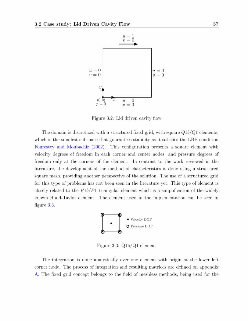
is flowing with a dimensionless velocity of u = 1, v = 0 , see figure 3.2. The behavior of
the fluid is different depending which Reynolds number is used.
3.2 Case study: Lid Driven Cavity Flow 37
Figure 3.2: Lid driven cavity flow
The domain is discretized with a structured fixed grid, with square Q1b/Q1 elements,
which is the smallest subspace that guarantees stability as it satisfies the LBB condition
Fourestey and Moubachir (2002). This configuration presents a square element with
velocity degrees of freedom in each corner and center nodes, and pressure degrees of
freedom only at the corners of the element. In contrast to the work reviewed in the
literature, the development of the method of characteristics is done using a structured
square mesh, providing another perspective of the solution. The use of a structured grid
for this type of problems has not been seen in the literature yet. This type of element is
closely related to the P1b/P1 triangular element which is a simplification of the widely
known Hood-Taylor element. The element used in the implementation can be seen in
figure 3.3.
Figure 3.3: Q1b/Q1 element
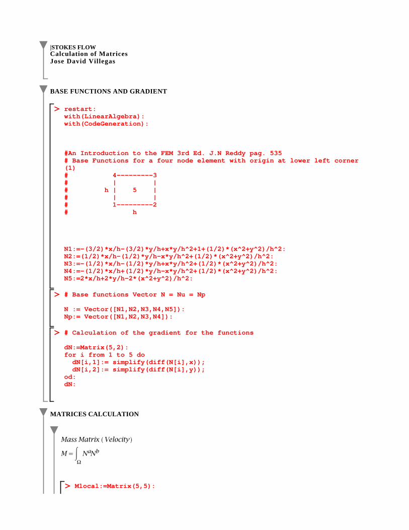
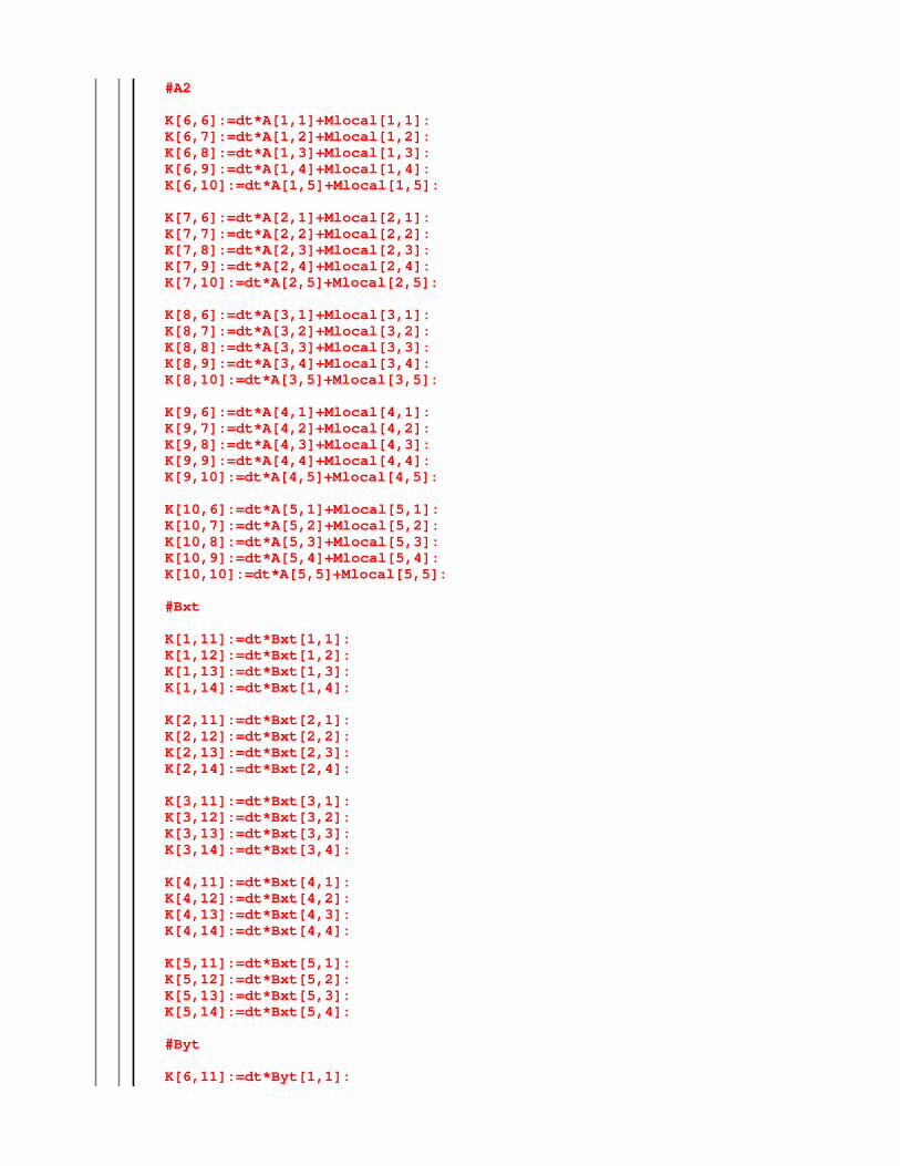
The integration is done analytically over one element with origin at the lower left
corner node. The process of integration and resulting matrices are defined on appendix
A. The fixed grid concept belongs to the field of meshless methods, being used for the
38 Solution of the NS Equation using the Lagrange-Galerkin method
treatment of problems in which the geometry of the domain changes in time. The method
has been used for phase change problems, elasticity problems, and it might be suitable for
problems involving fluid structure interaction. The advantage of using this approach is
because there is no need for remeshing, ideal for the characteristic curve implementation.
Regarding to the implementation, the points of the mesh are not stored but calulated
according the maximum dimensions of the domain. In this way, the mesh data (points
and connectivity) is only needed for post processing the results. In figure 3.4 a fixed mesh
of 32 x 32 elements can be seen. Observe that the node at the center of each element is
not plotted.
Figure 3.4: Finite Element Fixed Grid (32 x 32) elements
3.3 Results
The case study was solved using several values for the Reynolds number (Re=100,400,1000,3200)
and it is named as charNS. The results show good behavior of the flow when compared to
other experimental works done by Ghia et al. (1982) and openFOAM. The way to validate
the method is comparing the velocity profiles from a vertical and a horizontal line that
cross the geometric center of the cavity.
3.3 Results 39
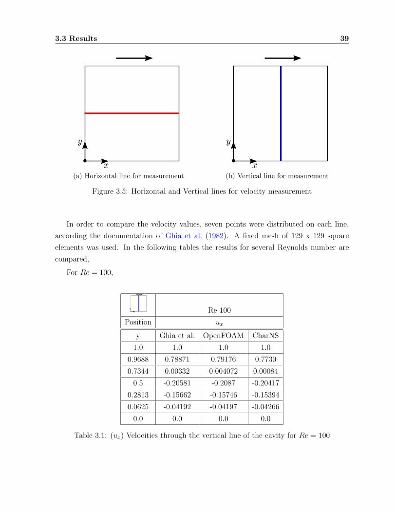
(a) Horizontal line for measurement (b) Vertical line for measurement
Figure 3.5: Horizontal and Vertical lines for velocity measurement
In order to compare the velocity values, seven points were distributed on each line,
according the documentation of Ghia et al. (1982). A fixed mesh of 129 x 129 square
elements was used. In the following tables the results for several Reynolds number are
compared,
For Re = 100,
Re 100
Position ux
y Ghia et al. OpenFOAM CharNS
1.0 1.0 1.0 1.0
0.9688 0.78871 0.79176 0.7730
0.7344 0.00332 0.004072 0.00084
0.5 -0.20581 -0.2087 -0.20417
0.2813 -0.15662 -0.15746 -0.15394
0.0625 -0.04192 -0.04197 -0.04266
0.0 0.0 0.0 0.0
Table 3.1: (ux) Velocities through the vertical line of the cavity for Re = 100
40 Solution of the NS Equation using the Lagrange-Galerkin method
Re 100
Position uy
x Ghia et al. OpenFOAM CharNS
1.0 0.0 0.0 0.0
0.9609 -0.07391 -0.07805 -0.08019
0.8594 -0.22445 -0.23354 -0.22714
0.5 0.05454 0.05751 0.05342
0.2266 0.17507 0.17901 0.1759
0.0703 0.10091 0.10336 0.10389
0.0 0.0 0.0 0.0
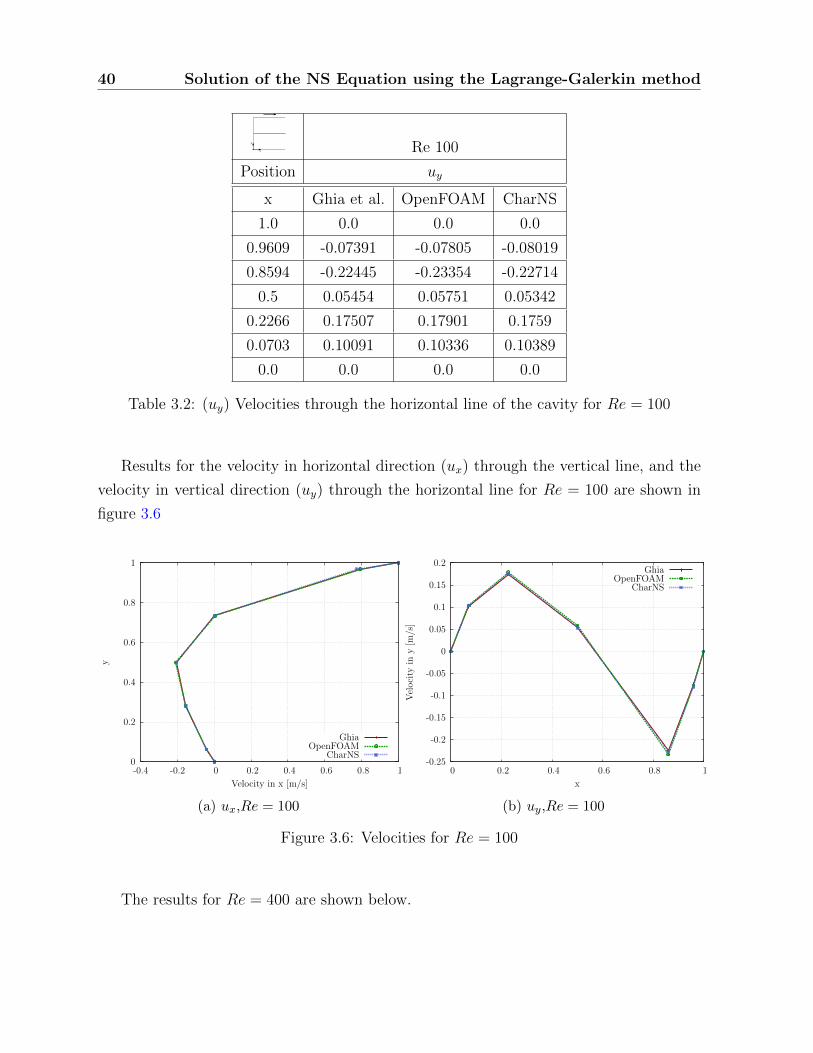
Table 3.2: (uy) Velocities through the horizontal line of the cavity for Re = 100
Results for the velocity in horizontal direction (ux) through the vertical line, and the
velocity in vertical direction (uy) through the horizontal line for Re = 100 are shown in
Table 3.4: (uy) Velocities through the horizontal line of the cavity for Re = 400
Re 400
Position ux
y Ghia et al. OpenFOAM CharNS
1.0 1.0 1.0 1.0
0.9688 0.68439 0.6863 0.6513
0.7344 0.16256 0.16149 0.1451
0.5 -0.11477 -0.11498 -0.1213
0.2813 -0.32726 -0.32625 -0.2993
0.0625 -0.09266 -0.09216 -0.0788
0.0 0.0 0.0 0.0
Table 3.3: (ux) Velocities through the vertical line of the cavity for Re = 400
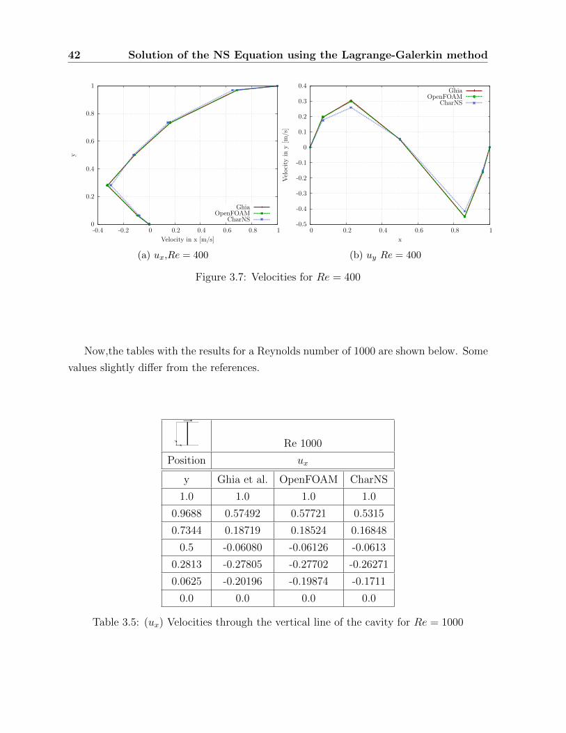
Plotting the results for Re = 400 in figure 3.7
42 Solution of the NS Equation using the Lagrange-Galerkin method
0
0.2
0.4
0.6
0.8
1
-0.4 -0.2 0 0.2 0.4 0.6 0.8 1
y
Velocity in x [m/s]
GhiaOpenFOAM
CharNS
(a) ux,Re = 400
-0.5
-0.4
-0.3
-0.2
-0.1
0
0.1
0.2
0.3
0.4
0 0.2 0.4 0.6 0.8 1
Vel
oci
tyin
y[m
/s]
x
GhiaOpenFOAM
CharNS
(b) uy Re = 400
Figure 3.7: Velocities for Re = 400
Now,the tables with the results for a Reynolds number of 1000 are shown below. Some
values slightly differ from the references.
Re 1000
Position ux
y Ghia et al. OpenFOAM CharNS
1.0 1.0 1.0 1.0
0.9688 0.57492 0.57721 0.5315
0.7344 0.18719 0.18524 0.16848
0.5 -0.06080 -0.06126 -0.0613
0.2813 -0.27805 -0.27702 -0.26271
0.0625 -0.20196 -0.19874 -0.1711
0.0 0.0 0.0 0.0
Table 3.5: (ux) Velocities through the vertical line of the cavity for Re = 1000
3.3 Results 43
Re 1000
Position uy
x Ghia et al. OpenFOAM CharNS
1.0 0.0 0.0 0.0
0.9609 -0.27669 -0.28819 -0.2681
0.8594 -0.42665 -0.42197 -0.39546
0.5 0.02526 0.02575 0.02555
0.2266 0.33075 0.32940 0.30655
0.0703 0.29012 0.29008 0.25719
0.0 0.0 0.0 0.0
Table 3.6: (uy) Velocities through the horizontal line of the cavity for Re = 1000
Plotting the results for Re = 1000 in figure 3.8
0
0.2
0.4
0.6
0.8
1
-0.4 -0.2 0 0.2 0.4 0.6 0.8 1
y
Veloccity in x [m/s]
GhiaOpenFOAM
CharNS
(a) ux,Re = 1000
-0.5
-0.4
-0.3
-0.2
-0.1
0
0.1
0.2
0.3
0.4
0 0.2 0.4 0.6 0.8 1
Vel
oci
tyin
y[m
/s]
x
GhiaOpenFOAM
CharNS
(b) uy,Re = 1000
Figure 3.8: Velocities for Re = 1000
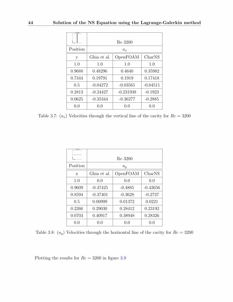
The last simulated case was Re = 3200, which means a flow in the transition regime,
almost turbulent. It can be seen that vortices are found without the inclusion of turbulence
models.
44 Solution of the NS Equation using the Lagrange-Galerkin method
Re 3200
Position ux
y Ghia et al. OpenFOAM CharNS
1.0 1.0 1.0 1.0
0.9688 0.48296 0.4640 0.35982
0.7344 0.19791 0.1919 0.17418
0.5 -0.04272 -0.03561 -0.04511
0.2813 -0.24427 -0.231938 -0.1923
0.0625 -0.35344 -0.36277 -0.2885
0.0 0.0 0.0 0.0
Table 3.7: (ux) Velocities through the vertical line of the cavity for Re = 3200
Re 3200
Position uy
x Ghia et al. OpenFOAM CharNS
1.0 0.0 0.0 0.0
0.9609 -0.47425 -0.4885 -0.42656
0.8594 -0.37401 -0.3628 -0.2737
0.5 0.00999 0.01372 0.0221
0.2266 0.29030 0.28412 0.23192
0.0703 0.40917 0.38948 0.28326
0.0 0.0 0.0 0.0
Table 3.8: (uy) Velocities through the horizontal line of the cavity for Re = 3200
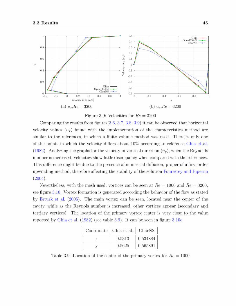
Plotting the results for Re = 3200 in figure 3.9
3.3 Results 45
0
0.2
0.4
0.6
0.8
1
-0.4 -0.2 0 0.2 0.4 0.6 0.8 1
y
Velocity in x [m/s]
GhiaOpenFOAM
CharNS
(a) ux,Re = 3200
-0.5
-0.4
-0.3
-0.2
-0.1
0
0.1
0.2
0.3
0.4
0.5
0 0.2 0.4 0.6 0.8 1
Vel
oci
tyin
y[m
/s]
x
GhiaOpenFOAM
CharNS
(b) uy,Re = 3200
Figure 3.9: Velocities for Re = 3200
Comparing the results from figures(3.6, 3.7, 3.8, 3.9) it can be observed that horizontal
velocity values (ux) found with the implementation of the characteristics method are
similar to the references, in which a finite volume method was used. There is only one
of the points in which the velocity differs about 10% according to reference Ghia et al.
(1982). Analyzing the graphs for the velocity in vertical direction (uy), when the Reynolds
number is increased, velocities show little discrepancy when compared with the references.
This difference might be due to the presence of numerical diffusion, proper of a first order
upwinding method, therefore affecting the stability of the solution Fourestey and Piperno
(2004).
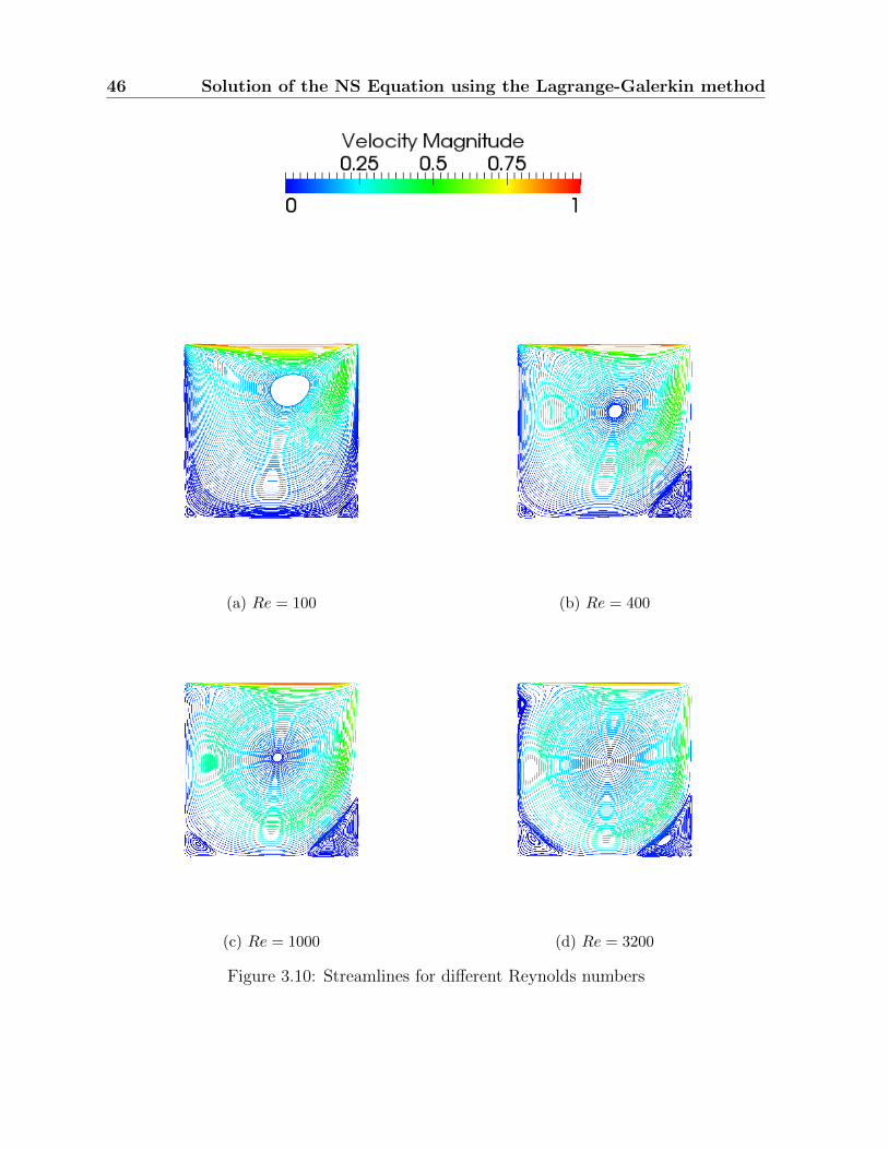
Nevertheless, with the mesh used, vortices can be seen at Re = 1000 and Re = 3200,
see figure 3.10. Vortex formation is generated according the behavior of the flow as stated
by Erturk et al. (2005). The main vortex can be seen, located near the center of the
cavity, while as the Reynols number is increased, other vortices appear (secondary and
tertiary vortices). The location of the primary vortex center is very close to the value
reported by Ghia et al. (1982) (see table 3.9). It can be seen in figure 3.10c
Coordinate Ghia et al. CharNS
x 0.5313 0.534884
y 0.5625 0.565891
Table 3.9: Location of the center of the primary vortex for Re = 1000
46 Solution of the NS Equation using the Lagrange-Galerkin method
(a) Re = 100 (b) Re = 400
(c) Re = 1000 (d) Re = 3200
Figure 3.10: Streamlines for different Reynolds numbers
3.4 Conclusion 47
3.4 Conclusion
The development of the Lagrange-Galerkin method is able to solve the Navier Stokes
equation for incompressible flow combining advantages from the Eulerian and Lagrangian
schemes, as it can be implemented on a fixed mesh avoiding the process of remeshing.
When using this method, transient problems can be solved efficiently using large timesteps
whenever the characteristic curve is sufficiently smooth, in other words, if it can be split
in small sections. Compared to the CBS scheme, the discretization process is much clearer
as it derives from a variational formulation of the Stokes problem and the material deriva-
tive is treated as a simple time derivative which can be discretized in a finite difference
manner. Moreover, the imposition of boundary conditions is also clearer because of the
appearance of these in the variational formulation in a natural way.
Regarding to the results, despite the existence of concordance with the calculated val-
ues and those reported on the references, when the Reynolds number is increased, the
values begin to differ, being necessary the change of the characteristic curve approxima-
tion to a second order scheme in order to lessen numerical dissipation. Another way to
improve the solution is by doing a mesh refinement on zones where vortices tend to ap-
pear. The main advantages of the method are the ability to handle the convective term in
a Lagrangian fashion, the clear variational formulation and the use of large timestepping.
Appendix A
Stokes flow: calculation of local
matrices
48
|STOKES FLOWCalculation of MatricesJose David Villegas
BASE FUNCTIONS AND GRADIENT
restart:with(LinearAlgebra):with(CodeGeneration):
#An Introduction to the FEM 3rd Ed. J.N Reddy pag. 535# Base Functions for a four node element with origin at lower left corner (1)# 4---------3# | |# h | 5 | # | | # 1---------2# h