86
SOLUTIONS OF THE TWO-DIMENSIONAL HELMHOLTZ EQUATION Robert S. Jones, Ph.D. November 5, 2004 1
SOLUTIONS OF THE TWO-DIMENSIONAL
HELMHOLTZ EQUATION
Robert S. Jones, Ph.D.
November 5, 2004
1
0 INTRODUCTION 2
0 INTRODUCTION
NOTE: This is a re-entry of my Ph.D. thesis I wrote in 1993 at The Ohio State University,
Physics Department. It is as close as practical to the original with some grammar fixes,
re-numbering, and some formatting changes.
–R.S. Jones, Autumn 2004
In this project, I examine the solutions of the two-dimensional Helmholtz equation within
several domains formed by piecing together identical 30◦-60◦-90◦ triangles. These shapes
were chosen partly because of their relation to the hexagonal region and partly because
they may be compared to the closed-form equilateral triangle eigenmodes. This study is
motivated by two important physical applications. The first is the quantum-mechanical,
three-body problem with one-dimensional infinite square wells {[4], [10]}. The second is
the electromagnetic waveguide problem [25]. Both applications involve essentially identical
mathematical formulations.
The Helmholtz equation plus the appropriate boundary conditions constitute the eigen-
value problem of the Laplacian,
∇2Ψ + λΨ = 0. (1)
The Helmholtz equation results from the Schrodinger equation for the quantum mechanical
problem {[30], for example} and from the Maxwell equations for the waveguide problems
{[11], for example}. Much physics is contained in the boundary conditions. In this project,
only Dirichlet and Neumann boundary conditions are considered. Specific boundary condi-
tions restrict the possible values (spectrum) of λ to a denumerable, infinite set (with a lower
bound).
Pedagogical as well as practical applications of the Helmholtz equation typically involve
domains for which the eigenfunctions Ψ and eigenvalues λ are well known in closed form.
The only two-dimensional domains for which complete sets of ‘exact’ or closed-form results
exist are the equilateral-triangle, the rectangle, the ellipse, and special cases of these (such as
the square, isosceles right triangle, circle, half circle, etc.). The rectangular and the elliptical
modes are unique in that they may be obtained by separation of variables. The triangular and
rectangular modes are similar in that they may be expressed as a finite sum of plane waves
0 INTRODUCTION 3
and that they may tile the plane using the Riemann-Schwarz reflection principle. There
exist no other two-dimensional domains for which complete sets of modes are expressible in
closed form, known or otherwise [35].
The closed-form equilateral triangle modes were first discovered by Lame in 1852 [16].
Curiously, these results have been left out of the modern curriculum; I have been able to
find only two textbooks which discuss these equilateral triangle modes {[22], [29]1}, despite
the fact that this problem provides a unique and elementary example of a non-separable
solution of the two-dimensional Helmholtz equation. Over the years, authors appear to
have ‘rediscovered’ these closed-form results in one form or another. Consequently, novel
derivations and interesting discussions are scattered throughout the literature. In addition
to [29] and [22], a list of modem references which refer to the closed-form modes includes
{[15], [31], [4], [5], [21], [10], [9], [26], [8], [13], [34], [20], [25], [35], [39]}.2 Appendix A of this
thesis collects important results.3
Interesting physical systems exist for which solutions within other domains are appro-
priate. For the three-body problem, the important regions include the regular hexagon and
the 60◦ rhombus, both satisfying Dirichlet boundary conditions. The application to the
waveguide problem is more practical and less pedagogical than the three-body square-well
problem. Also, it is slightly more general since more regions - with both Dirichlet and
Neumann boundary conditions - are studied. (Here, the ‘region’ or ‘domain’ refers to the
cross-section of the guide.) Indeed, five domains are considered, each of which is formed by
piecing together identical 30◦-60◦-90◦ triangles. (The hexagon also satisfies this property.)
A large part of this dissertation is concerned with the numerical solution of the eigenvalue
problem. Two different and independent methods of solutions are used, both very success-
fully.4 The first is a combination of the imaginary time-step [12] and finite-difference [1]
1However, see [25] regarding Ref. [29].2Much thanks to P. L. Overfelt for pointing out some of these to me.3I also provide my own discussion, including a simple and practical algorithm for tabulating and clasifying
the modes.4Other methods were tried and abandoned because of moderate or low success. For example, Rayleigh-
Ritz, five parameter polynomial trial-functions provided upper-bounds to only the very lowest eigenmodes
with only three or four digit accuracy in the eigenvalue.
0 INTRODUCTION 4
(ITS/FD) methods, with which 69 regular hexagon modes with Dirichlet boundary condi-
tions were computed to at least five digit accuracy in the eigenvalue. The second method
of solution is the point-matching or collocation method, whereby an exact solution of the
Helmholtz equation is made to satisfy the boundary conditions approximately.5 The TE
(Neumann) and TM (Dirichlet) modes6 of the regions of Fig. 6 (Chapter 3) are divided up
into eight symmetry classes, four of which correspond to the closed-form modes. A total
of 26 non-closed-form modes are computed to a very high (and quite possibly an unprece-
dented) precision. For example, using the point-matching method with seventy matching
points, I have determined the cutoff wavenumber of the lowest regular hexagon TM mode
(with unit-length edges) to lie between 2.674946522 and 2.674946580; whereas (to my knowl-
edge), the previous best result [4] was 2.67495 (unbounded) using Richardson extrapolation
of finite-difference results.
Perhaps the strongest advantages of both the ITS/FD and the point-matching methods
are that they are simple to implement and guaranteed to work reliably. The application
of both methods to the problem at hand was straightforward. With the ITS/FD method,
a complete FORTRAN program was developed within one week. Computation of the 69
hexagon modes to the desired precision required hundreds of CPU hours on the VAX cluster
and was completed within about two months (real time). With the point-matching method,
the symbolic/numerical programming language MAPLE was used. MAPLE programs were
developed and run within days, requiring only tens of CPU hours on the VAX cluster for
comparable results. The chosen languages were well suited to each method.7
It appears that the point-matching method is far superior to the ITS/FD method. First,
as suggested above, the amount of computer effort is significantly less for the point-matching
method. Second, the ITS/FD method required that the values at each of the 15,000 grid
5As reviewed in Chapter 3, this is done by enforcing the boundary conditions at a finite set of points on
the boundary.6The notation ‘TE’ and ‘TM’ stands form respectively transverse electric and transverse magnetic waveg-
uide modes.7It may be mentioned that MAPLE is an interpretive language which can perform arithmetic operations
to arbitrary precision, implemented in software; FORTRAN is a compiled language and numerical precision
is (essentially) limited to that of the hardware precision.

0 INTRODUCTION 5
points for each eigenfunction be stored – thus requiring a significant amount of disk space.
The point-matching method did not require any storage of the eigenfunctions. Related to this
is the disparate number of parameters used to represent each eigenfunction: ITS/FD (N ≈5, 000 corresponding to the number of grid points) vs point-matching (N < 50 corresponding
to the number of matching points) for comparable precision within the 30◦-60◦-90◦ triangle.
Third, with the ITS/FD method the precision and accuracy of each eigenmode depended
upon the precision and accuracy of the lower modes. The point-matching method was used to
determine each mode, independent of any other mode. Finally, and probably most important,
the point-matching method was used to provide very tight upper and lower bounds to each
eigenvalue. Although it is possible to estimate more accurately the eigenvalues using the
Richardson extrapolation,8 it is difficult to bound the eigenvalues using the finite-difference
method {[13], Sec. 141}. Furthermore, nothing analogous to ‘Richardson extrapolation’
exists for the eigenfunction.
Of course, using independent methods has an advantage because results can be compared.
Thus, some duplication in work paid off in that estimates of precision using the ITS/FD
method were obtained. Some other checks of precision included comparison of the numerical
results to closed-form results, and comparison of degenerate modes within separate symmetry
classes. Ten of the lowest 69 hexagon modes correspond to closed-form equilateral triangle
modes.
This thesis is logically divided into four chapters. First, I discuss the physics of the
quantum-mechanical three-body problem. It is shown that the one-dimensional three-body
problem with infinite square-well potentials is equivalent to the Dirichlet eigenvalue problem
of the hexagon or the rhombus – plus the trivial center-of-mass motion. The usual classi-
fication scheme for the eigenmodes according to permutation symmetry and parity is also
discussed. This is especially useful in understanding the relation between the hexagon and
rhombus modes and the three-body system. Appendix B collects some useful coordinate
transformation results.
Second, I describe the algorithm of the ITS/FD method and its application to the hexagon
8This is done by calculating the eigenvalues at low grid resolution and extrapolating to the limit of infinite
grid resolution.

0 INTRODUCTION 6
eigenmodes. The lowest 69 eigenfunctions results are reported using contour plots. These
contour plots are particularly interesting because they reveal both the complexity and an
inherent beauty of the problem. Because of their voluminous nature, the pictures are given
in Appendix C. The (Dirichlet) rhombus modes are not solved using this method.
Third, the waveguide problem is discussed. A relation between the modes of the various
regions shown in Fig. 6 (Chapter 3) is derived, based on the symmetry properties, and
boundary conditions of the respective eigenvalue problems. This is an interesting result based
on elementary considerations. Finally, I describe the point-matching method as a way to solve
the eigenvalue problem and how it is used to solve the three-body problem (Chapter 1) and
the waveguide problem (Chapter 3). To begin, the eigenfunction is expanded in a Fourier-
Bessel series. Next, the point-matching method provides an algorithm to determine the
expansion coefficients and the eigenvalue. I apply this method to each mode with minimal-
order computations to gain insight into how it works. Then, I apply it using high-order
computations to the non-closed-form modes. In this process, two important properties are
revealed. As mentioned above, one property is that relatively tight bounds to the eigenvalues
can be obtained. The other property is that a simple relation exists between the expansion
coefficients.

1 THE THREE-BODY PROBLEM 7
1 THE THREE-BODY PROBLEM
1.1 Preliminaries
I begin by posing the following physical problem:
Consider the quantum-mechanical three-body problem with one-dimensional in-
finite square wells. For simplicity, assume the particles are of equal mass and the
range of each square well is identical. Determine the eigenfunctions and eigen-
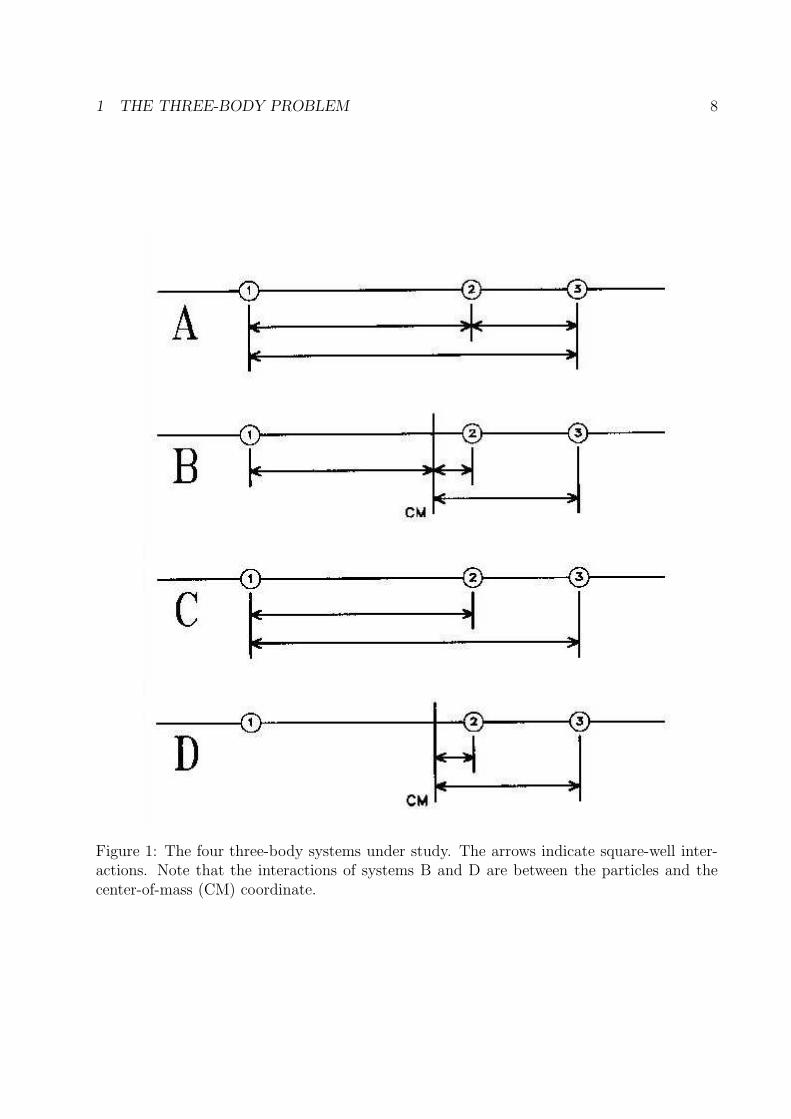
values of the four possible variants illustrated in Fig. 1. In systems A and C,
the bonds occur between the pairs of particles; in systems B and D, the bonds
exist between each particle and the center-of-mass location. (Systems A and B
include three bonds, while systems C and D include only two bonds.) Classify the
eigenmodes according to the symmetry group of each system and determine geo-
metrical and accidental degeneracies, if present. Also, determine any closed-form
results, if possible.
Elementary quantum texts quite often make use of the infinite square well as a model
to introduce many physical concepts such as bound states and spectra. This is primarily
because the relative simplicity of the mathematics does not obscure the physics. Curiously,
the texts rarely – if ever – go beyond the one- or two-body problem, despite the fact that
most real systems consist of several to many particles. The physical problem posed above
is perhaps the most elementary extension of introductory considerations since it contains
three particles, Despite its benign appearance, this three-body paradigm is not trivial, and
understanding this model provides a window into the very interesting world of multi-particle
systems.
This chapter is devoted to examining the solution of the systems A-D. The solution con-
sists in first separating the (trivial) center-of-mass motion from the internal dynamics. Then,
for each system, the ‘internal’ eigenstates are determined by solving the two-dimensional
Helmholtz equation - with Dirichlet boundary conditions - within either the regular hexagon
{[7], [4]} (systems A and B) or the 600 rhombus [32] (systems C and D). Invariances or
symmetries of the systems consist of spatial inversion (parity) and particle permutation.
1 THE THREE-BODY PROBLEM 8
Figure 1: The four three-body systems under study. The arrows indicate square-well inter-actions. Note that the interactions of systems B and D are between the particles and thecenter-of-mass (CM) coordinate.

1 THE THREE-BODY PROBLEM 9
Consequently, the states are classified according to the irreducible representations of these
groups. In addition, the symmetry properties directly translate into simple geometrical
operations on the hexagon or rhombus eigenmodes.
It should be emphasized that none of the systems A-D is equivalent to the system con-
sisting of three independently interacting particles, each of which interacts with a com-
mon one-dimensional infinite square well. In this system - call it E - the center-of-mass is
fixed (i.e., not free to move) and the states are equivalent to the Dirichlet modes within
a three-dimensional rectangular Parallelepiped.9 Nevertheless, contrasting and comparing
these systems is instructive.10 The central-potential problem E is the direct product of three
one-body problems; therefore, the states of E are products of closed-form single-particle
states – or linear combinations of such products. As with systems A through D, the states
of E may be classified according to the ‘three-body symmetry groups,’ i.e., permutations
(where appropriate) plus inversion.
A most interesting feature of the systems A through D is that some of the three-body
states are expressible in closed form. These closed-form states correspond to those hexagonal
or rhombic modes in which nodal lines divide the domain into equilateral triangles. This
is because the equilateral triangle modes are expressible in closed form. Physically, these
closed-form modes are shown to correspond to the fully antisymmetric states of system A,
the fully symmetric states of system B, the states antisymmetric in particles 2 and 3 of
system C, and the states antisymmetric in particle 1 with respect to the center-of-mass of
system D. Appendix A examines the closed-form equilateral triangle modes and includes
references.
9The Dirichlet problem within a rectangular parallelepiped (with various applications) is treated in many
elementary texts such as {[30], [23], [11], [28]}. if the particles are identical, the geometry is a cube.10Curiously, Ref. [8] transforms some three-dimensional cubical modes (antisymmetric states of the three-
body problem of type E) into the two-dimensional equilateral triangular modes (antisymmetric states of
the three-body of type A) simply by transforming the coordinates. Although mathematically correct, the
physical argument that systems A and E are equivalent is faulty. For example, the spectra, degeneracies,
etc., are very different.

1 THE THREE-BODY PROBLEM 10
1.2 Setting-up the Problem
In this section, the Schrodinger equation is separated according to the internal and center-of-
mass motions. The canonical form of the problem is described. It is shown that the internal
Schrodinger problem with infinite square wells is equivalent to the Dirichlet Helmholtz prob-
lem inside a regular hexagon or a 60◦ rhombus.
For equal mass particles, the Schrodinger equation is
− h2
2m
[∂2
∂r21
+∂2
∂r22
+∂2
∂r23
]Ψ(r1, r2, r3) = [ETOT − V ] Ψ(r1, r2, r3) (2)
where the translationally invariant potential V is one of
VA = v(r1 − r2) + v(r2 − r3) + v(r3 − r1); (3)
VB = v(r1 −RCM) + v(r2 −RCM ) + v(r3 − RCM); (4)
VC = v(r1 − r2) + v(r3 − r1); (5)
VD = v(r2 −RCM) + v(r3 −RCM ); (6)
and where the center-of-mass location is
RCM =r1 + r2 + r3
3. (7)
The one-dimensional infinite square well potential is defined by
v(x) =
0 if |x| < a
∞ if |x| > a, (8)
where a is the range of the force. The boundary conditions on the wavefunction are imposed
by requiring Ψ ≡ 0 unless V = 0. This occurs only if all of the arguments of the v’s have
magnitude less than a. For example, ΨA ≡ 0 unless VA = 0. Thus, if either |r1 − r2| > a,
|r2 − r3| > a, or |r3 − r1| > a, then ΨA ≡ 0.
The distance between a particle coordinate and the center-of-mass of the entire system
can be related to the distance between that particle and the center-of-mass of the remaining
pair, for example,
r1 − RCM ≡2
3
(r1 −
r2 + r3
2
). (9)

1 THE THREE-BODY PROBLEM 11
This is important because it easily generalizes problems B and D – with little or no additional
work – to those problems in which each particle interacts with the center-of-mass of the
remaining pair.
Since the center-of-mass is free to move, the eigenfunction Ψ is not normalizable. How-
ever, using the considerations reviewed in Appendix B, the center-of-mass motion is easily
isolated from the internal dynamics. The internal eigenfunction is normalizable and has a
discrete bound-state spectrum. It is this internal problem which is interesting.
Let the letters (i, j, k) represent a cyclic permutation of (1, 2, 3). Using the equal mass
condition and the transformations of Appendix B; namely11
xi =
√1
2(rj − rk) ; (10)
yi = −√
3
2(ri −RCM ) = −
√2
3
(ri −
rj + rk2
); (11)
zi =√
3RCM ; (12)
the Schrodinger equation is transformed into the two-dimensional version
−[∂2
∂x2+
∂2
∂y2
]ψ(x, y) =
2m
h2 [E − V ]ψ(x, y) (13)
where
Ψ(r1, r2, r3) = e±iκzψ(x, y) ; (14)
E = ETOT −h2κ2
2m. (15)
Note that E is the internal energy and assumes discrete positive values. Also note that if no
subscripts appear on x or y, any one of the three sets of coordinates can be used.
The parameter κ is proportional to the center-of-mass momentum PCM = p1 + p2 + p3,
since κ z = PCMRCM . Thus
κ =PCM√
3(16)
11Appendix B treats the general mass case and it is convenient to include the masses in those transfor-
mations. Here, it is more convenient to factor the mass out and not include it in the transformations. One
easy way to transcribe the results of Appendix B to this section is to first assume that m = mi = 1, and in
the end restore m 6= 1.

1 THE THREE-BODY PROBLEM 12
The internal energy is thus
E = ETOT −h2P 2
CM
2 · 3m (17)
which may have been obtained directly from elementary principles. The fact that κ can
assume arbitrary values demonstrates that the center-of-mass motion forms a doubly degen-
erate continuum of states. Indeed, the plus or minus sign on the exponential corresponds to
the fact that the bound system can be traveling as a plane wave to the right (e+iκz) or left
(e−iκz) in the one-dimensional particle configuration space. With this said, continue with
the more interesting internal problem.
Each point of the two-dimensional configuration space with coordinates (x1, y1), (x2, y2),
or (x3, y3) represents an internal configuration of the three-body system. These coordinates
can be expressed in terms of each other. Expressing the ‘2’ and ‘3’ coordinates in terms of
the ‘1’ coordinates,
x2 = −1
2x1 +
√3
2y1 (18)
y2 = −√
3
2x1 −
1
2y1 (19)
x3 = −1
2x1 −
√3
2y1 (20)
y3 = +
√3
2x1 −
1
2y1 (21)
These transformations correspond to rotations by ±2π/2 in the plane. Fig. 2 shows, these
coordinates.
Each sixty degree wedge defined by the three y-axes specifies an ordering of the particles
along the one-dimensional particle configuration space. When ‘crossing’ the yi-axis, the
particles j and k switch places. To determine the orderings, it is only necessary to use
xi ∝ rj − rk, and decide if xi > 0 or if xi < 0 for i = 1, 2, 3 within each 60◦ wedge.
These considerations are helpful in understanding the symmetry of the states. For example,
exchanging the particles at rj and rk, corresponds to the reflection (xi, yi)→ (−xi, yi). This
is described in more detail in the next section.
The potential V is translationally invariant; therefore, it does not depend on RCM . In-
deed,
VA = v(γx1) + v(γx2) + v(γx3); (22)

1 THE THREE-BODY PROBLEM 13
VB = v(γ′y1) + v(γ′y2) + v(γ′y3); (23)
VC = v(γx2) + v(γx3); (24)
VD = v(γ′y2) + v(γ′y3); (25)
where (for convenience)
γ ≡√
2 and γ′ ≡√
2
3(26)
For the infinite square well potentials, the regions in which V = 0 define polygons in the
xy-plane:
VA = 0 only if |xi| < a/γ for i = 1, 2, 3;
VB = 0 only if |yi| < a/γ′ for i = 1, 2, 3;
VC = 0 only if |xi| < a/γ for i = 2, 3;
VD = 0 only if |yi| < a/γ′ for i = 2, 3.
(27)
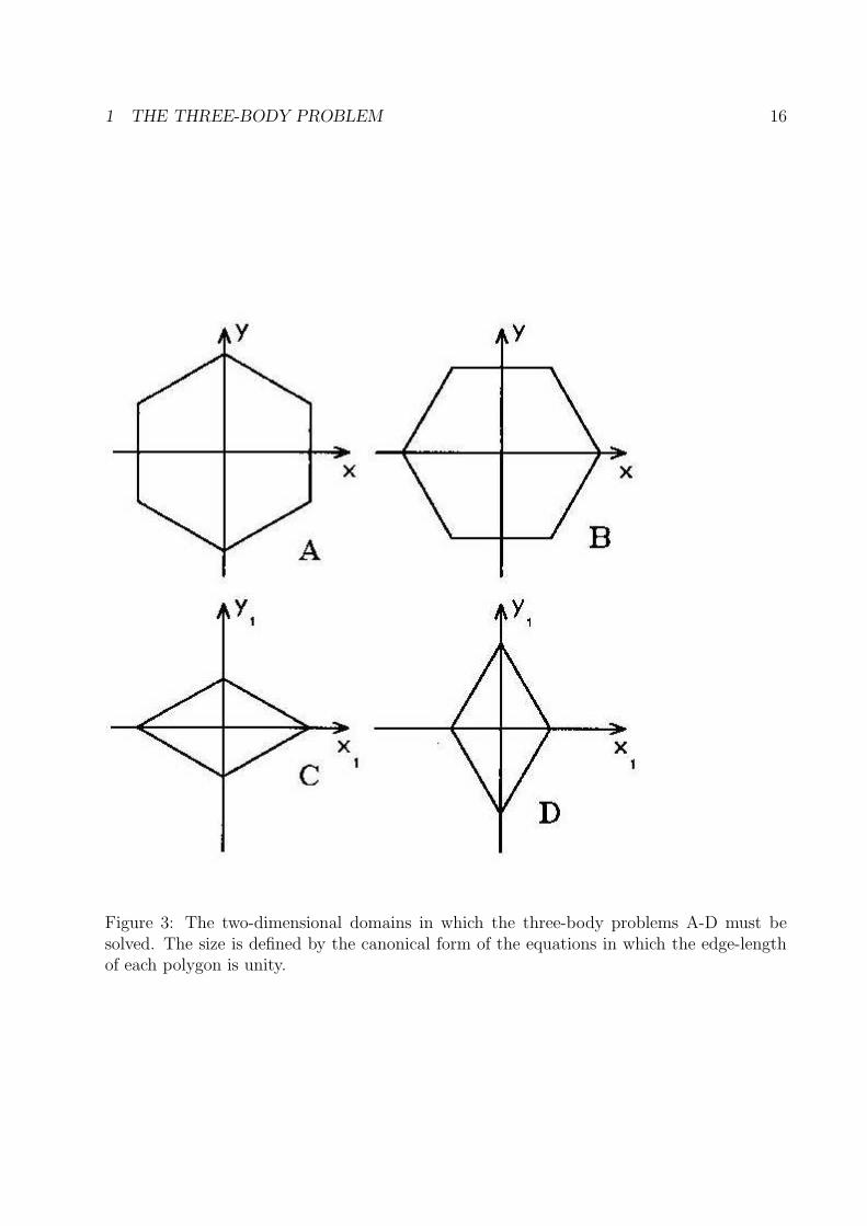
To draw the polygons, draw the lines xi = ±a/γ for VA and VC , and yi = ±a/γ′ for VB and
VD. These shapes are shown in Fig. 3. For VA and VB, the region is a regular hexagon, and
for VC and VD the region is a 60◦ rhombus. Note that – as described below – the edge length
of each polygon is chosen to be unity.
The internal problem is thus reduced to that of the Helmholtz equation, with Dirichlet
boundary conditions, within the regular hexagon or the 60◦ rhombus. To express the problem
in a canonical form, first let k be the eigenparameter such that Eq. (13) becomes
[∂2
∂x2+
∂2
∂y2+ k2
]ψ(k; x, y) = 0. (28)
This eigenparameter k is related to the internal-energy eigenvalue according to
E =h2k2
2m. (29)
Of course, the eigenfunction ψ is constrained to vanish on the edge of the polygonal domains
shown in Fig. 3.
Next, the domains are chosen to have unit edge-length in the xy-plane. This corresponds
to fixing the value of a according to, respectively,
system A : |rj − rk| = γ|xi| < a = γ√
32
⇒ aA ≡√
3
2; (30)

1 THE THREE-BODY PROBLEM 14
Figure 2: The internal two-dimensional configuration space of the one-dimensional three-body problem.

1 THE THREE-BODY PROBLEM 15
system B : |ri −RCM | = γ′|yi| < a = γ′√
32⇒ aB ≡
√1
2; (31)
system C : |rj − rk| = γ|xi| < a = γ√
34
⇒ aC ≡1
2
√3
2; (32)
system D : |ri −RCM | = γ′|yi| < a = γ′√
34⇒ aD ≡
1
2
√1
2. (33)
These are the conditions on the range which lead to unit-edged polygons. Note that the
canonical ranges of the systems C and D are one half those of systems A and B respectively.
Of course, it is possible to extend the results to an arbitrary ‘range’ of the potential by
using the scale invariance of the Helmholtz problem. Thus, if we transform the problem
according to (x, y)→ (βx, βy), where β is an arbitrary scale factor, then the range and the
eigenparameter change according to
a→ a′ = βa and k → k′ =k
β(34)
This corresponds to changing the edge-length of the respective polygon by a factor of a.
In the Chapters 2 and 4, the numerical solutions of these problems for 0 < k < 20 are found
to a very high precision. It is determined that there are 69 hexagon states and 21 rhombus
states in this range of k, some of which are expressible in closed form.
It may be mentioned that the present problem is equivalent to that in which a particle
is confined by the two-dimensional domains of the regular hexagon and the 60◦ rhombus.
The results may be used to examine the correspondence principle relating the classical and
quantal systems of the hexagonal and rhombical ‘billiard’ problems [35], for example.
In the next section, the symmetry of the states examined and a classification scheme is
described.
1.3 Classification of the Three-Body States
The group under which the internal three-body system is invariant consists of particle per-
mutations and spatial inversion. For systems A and B, the permutations include all three
particles, while for systems C and D, particle 1 is left out of the permutations. For two
particles, the group is S2 and consists of only the transposition of particles 2 and 3. For
1 THE THREE-BODY PROBLEM 16
Figure 3: The two-dimensional domains in which the three-body problems A-D must besolved. The size is defined by the canonical form of the equations in which the edge-lengthof each polygon is unity.
1 THE THREE-BODY PROBLEM 17
three particles, the permutation group is S3 and consists of six operations. All four systems
are invariant under inversion i.
The states are classified according to the irreducible representations of the symmetry
group. First, states are even or odd under inversion, which corresponds to the parity of the
state. A superscripted, parenthesized plus or minus sign is used to indicate the parity of a
quantity.
Regarding the two-dimensional configuration space (x, y), each axis may be either even
or odd. In general, an axis or other straight line is ‘odd’ if there is a node in the eigenfunction
along this line; while it is ‘even’ if contour lines of the eigenfunction cross this axis at right
angles.
The Riemann-Schwarz reflection principle can be used to continue a harmonic function12
through a straight even or odd edge. Indeed, if x = 0 is an even or odd line for the
eigenfunction ψ(x, y), then ψ(−x, y) = ±ψ(x, y) respectively. This process can be repeated
as long as the eigenfunction remains single valued.
Under the permutation of particles 2 and 3, systems C and D are either even or odd.
Thus, in terms of the rhombus modes, the symmetry across the y1, axis is either even or odd,
since xi ∝ r2 − r3. The closed-form states are those states of system C which are odd under
(x1, y1)→ (−x1, y1) and those states of system D which are odd under (x1, y1)→ (x1,−y1).
This is easy to visualize since in both cases the rhombus is divided into equilateral triangles.
Together with inversion, the four symmetry classes of the rhombus states are obtained by
specifying the evenness or oddness of the x and y axes.
Chapter 3 discusses the rhombus modes in more detail using waveguide language. Chap-
ter 4 examines the lowest 21 rhombus eigenmodes (with Dirichlet boundary conditions)
numerically using the point-matching method and closed-form results.
Under permutations, systems A and B are fully symmetric S, fully antisymmetric A, or
mixed M. The mixed states come in degenerate pairs that are13 respectively odd and even
under permutations of particles 2 and 3. Since x1 ∝ r2−r3 and y1 ∝ r1− (r2 +r3)/2 are also
odd and even respectively under this transformation, we can label the mixed states using the
12I.e., any solution of Eq. (28).13or ‘can be made’

1 THE THREE-BODY PROBLEM 18
notation Mx and My. Thus, if an eigenfunction transforms like x1 (y1) under permutation
of particles 2 and 3, i.e. (r1, r2, r3) → (r1, r3, r2), and is a ‘mixed’ state, then it is classified
under Mx (My).
The symmetric and antisymmetric states are easy to identify. These are the states with
respectively all even or all odd lines along each of the three y axes. Indeed, if a state
is symmetric it must not change sign under any particle permutation. The transposition
of particles j and k, of course, corresponds to the transformations (xi, yi) → (−xi, yi) for
i = 1, 2, 3; since xi ∝ rj − rk and yi ∝ ri − (rj + rk)/2.
Thus, there are eight possible types of the ‘hexagon’ states. They are S (+), S(−), A(+),
A(−), M(+)x , M(−)
x , M(+)y , and M(−)
y . The hexagon contour plots shown in Appendix C are
classified using the system A. The states of system B are trivially obtained by rotating each
hexagon by ninety degrees.
There are several characteristics common to all hexagon states of a given type or classifi-
cation. Quite simply, these can be identified at-a-glance by noting the symmetry of the state
under reflection through the xi and yi axes. For example, those states which have nodes
connecting all three pairs of opposite vertices divide the hexagon into equilateral triangles.
These hexagon modes correspond to closed-form modes (Appendix A).
To classify the states of either system A or B, use these rules. With each contour plot
listed in Appendix C,14 choose the first one occurring in this list:
• S(+): All xi and yi are even;
• S(−): All xi are even and all yi are odd;
• A(+): All xi and yi are odd;
• A(−): All xi are odd and all yi are even;
• M(+)x : Only x1 and y1 are odd;
• M(−)x : Only x1 is odd and y1 is even;
14Caution: The classification of the states listed in Appendix C is for the system A. Thus, a symmetric
odd-parity system-A state corresponds to an antisymmetric odd parity system-B state; only S (−)is given in
the label.

1 THE THREE-BODY PROBLEM 19
• M(+)y : Only x1 and y1 are even;
• M(−)y : Only x1 is even and y1 is odd.
Thus, for example, if a hexagon mode is even in every x and every y axis, it corresponds
to a symmetric, even parity state.
Only the antisymmetric states (of either parity) of system A are closed form. Only the
symmetric states (of either parity) of system B are closed form. For values of k < 20, there
is no accidental degeneracy.
In systems A and B, the mixed modes come in pairs, each member of which has the same
parity, viz., (M(+)x , M(+)
y ) and (M(−)x , M(−)
y ). In system A, the antisymmetric states come
in degenerate pairs due to a geometrical symmetry of the equilateral triangle. These pairs
of states have opposite parity, viz,, (A(+), A(−)). Likewise, the geometrically degenerate
symmetric states of system B come in pairs with opposite parity, (S (+), S(−)).

2 NUMERICAL SOLUTION OF THE HEXAGON MODES 20
2 NUMERICAL SOLUTION OF THE HEXAGON MODES
“Numerical Analysis is partially a science and partially an art, and short of writ-
ing a textbook on the subject it has been impossible to indicate where and under
what circumstances the various formulas are used or accurate, or to elucidate the
numerical difficulties to which one might be led by uncritical use.”
- P. J. Davis and L. Polonsky {[1], page 877}
2.1 Preliminaries
In this chapter, I discuss the method by which I numerically solved for the Dirichlet modes
within the regular hexagon. The method is a combination of the imaginary-time-step (ITS)
and the finite-difference (FD) [1] procedures. The ITS algorithm is an iterative, relaxation
method whereby the eigenfunctions and eigenvalues are determined. Actual numerical rep-
resentation of the eigenfunctions using two-dimensional arrays require that a FD procedure
be used. I refer to the combination of these methods as the ‘ITS/FD’ procedure.15
This document lists no FORTRAN code since such inclusion (I believe) would be of
limited utility. However, the algorithm is presented in such a way that translation into your
favorite computer language is elementary. This is more useful since many of the techniques
discussed here are applicable to a whole class of eigenvalue problems of which the bound-state
Schrodinger problem is only one.
Using the ITS/FD procedure, 69 of the hexagon modes were determined. The numerous
contour plots are given in Appendix C for easy reference. The modes are divided up into
four symmetry classes according to the symmetry along the x and y axes. The eigenvalues
were computed to more than five digits in precision. Tables ????? 2-5 collect the numerical
results. For comparison, other published results [4], the point-matching results (Chapter
IV), and closed-form results (Appendix A) are included in these tables.
Regarding the accuracy of the hexagon modes, Ref. [13] (page 178) suggests that the
15The techniques of the ITS/FD algorithm as described in this chapter were taught to me by Dave Wasson,
to whom I owe much thanks. A recent paper which discusses the imaginary-time-step procedure can be found
in [12].
2 NUMERICAL SOLUTION OF THE HEXAGON MODES 21
non-closed-form results of [4] should be recomputed.16 My results do provide such a re-
computations and a comparison shows that the relative difference is less than 10−5. (For the
6-EE state, the relative discrepancy ∆k/k is the greatest at 8× 10⁻⁶.) In addition, the very
tight bounds obtained using the point-matching method (Chapter ??????IV) are also useful
for comparison; however, not all hexagon modes were computed this way.
2.2 The Eigenvalue Problem
The general eigenvalue problem and its desired solution are presented in the usual form. Let
H be the time-independent Hamiltonian of a system; then the orthonormalized eigenfunc-
tions ψns and the corresponding eigenvalues En of H satisfy the following relations,
Hψns = Enψns (35)
〈ψns|ψn′s′〉 = δnn′δss′ (36)
0 < E1 < E2 < · · · (37)
n = 1, 2, 3, · · · (38)
s = 1, 2, 3, · · · , gn gn is the multiplicity of En (39)
The inner product 〈f |g〉 of two well-behaved functions f and g is appropriate to the function
space under consideration. Regarding Eq. (37), it is tacitly assumed that the spectrum of H
has a lower bound. Thus, an inconsequential constant may be added to H (without changing
the physics) so that Eq. (37) is satisfied. Of course, the lower bound of the hexagon spectrum
is zero; therefore, this is not a problem.
Four symmetry classes are obtained by applying the symmetry conditions (Dirichlet
or Neumann) along the x and y axes. This division of the modes is convenient because
it separates the geometrically degenerate modes according to a simple rule.17 A useful
byproduct of doing this is that modes within separate computations may be compared. For
example, if two degenerate mixed modes agree in the eigenvalue only to d digits, we can be
confident that the eigenvalue may not be precise to more than d digits.
16This is because [4] used an incorrect Richardson extrapolation formula. Since I did not use Richardson
extrapolation, I can not make the same mistake.17Imposing the edge conditions along the x and y axes is relatively straightforward.

2 NUMERICAL SOLUTION OF THE HEXAGON MODES 22
Figure 4: The region in which the Helmholtz equation is solved. Also shown are the gridpoints (N = 5) used in the finite-difference algorithm.

2 NUMERICAL SOLUTION OF THE HEXAGON MODES 23
In the first quadrant of the hexagonal domain shown in Fig. ????4, the relevant equations
for the hexagon modes are
H = −[∂2
∂x2+
∂2
∂y2
](40)
〈f |g〉 =∫ √3/2
0dx
∫ 1−x/√
3
0dyf(x, y)g(x, y) (41)
There are four edges along which conditions must be imposed. The Dirichlet conditions
along an odd edge are imposed by requiring that the eigenfunction vanish along that edge.
The Neumann conditions along an even edge are imposed by requiring that the normal
derivative of the eigenfunction vanish across that edge. The actual method of imposing the
edge conditions depends upon the representation of the eigenfunction.
Let Px and Py be operators that reflect an eigenfunction through the x and y axes,
respectively. Then,
Pxψ(x, y) = ψ(−x, y) = ±ψ(x, y) ⇒
ψ|y=0 ≡ 0 (ψ odd in x)
∂ψ∂x|y=0 ≡ 0 (ψ even in x)
(42)
Pyψ(x, y) = ψ(x,−y) = ±ψ(x, y) ⇒
ψ|x=0 ≡ 0 (ψ odd in y)
∂ψ∂y|x=0 ≡ 0 (ψ even in y)
(43)
These symmetry relations are easily imposed along the x and y axes.
The inversion operator Q is obtained by successively operating with Px and Py (in either
order) on the eigenfunction. The parity of the eigenfunction is thus related to the eigenvalues
of Px and Py. Let ψ(q)(x, y) be an eigenfunction of Q = PxPy; then
Qψ(q)(x, y) = PxPyψ(q)(x, y) = ψ(q)(−x,−y) = qψ(q)(x, y) (44)
where q = ±1 is the parity.
I use an ordered pair of letters out of ‘E’ for even and ‘O’ for odd to form the notation
whereby each state is classified according to the symmetry under Px and Py, respectively.
Thus the four possibilities: ‘EE’, ‘EO’, ‘OE’, and ‘OO’. Each of these classifications can easily
be related to the three-body systems A and B. The classification scheme is summarized in
Table 2. Note that the EE and OO states have even parity and the EO and the OE states
have odd parity.

2 NUMERICAL SOLUTION OF THE HEXAGON MODES 24
Table 1: Classification scheme of the hexagon States as they relate to the three-body sys-tems A and B.
S(+) M(+)y M(+)
x A(+) A(−) M(−)x M(−)
y S(−)
EE AB AB
OO AB AB
OE A A B B
EO B B A A
This division of states separates geometrically degenerate states and is significant for two
reasons. The first is that degeneracies are removed from each computation. For example, a
tower of EE modes can be computed in which each state is not degenerate with any other
state within this EE tower.18 The second is that different computations can be compared. If
fact, it is possible to compare each of the four towers – from the lowest states to the highest –
by linking degenerate modes. The degenerate pairs must have the same eigenvalue. Thus
for system A, the (A(+), A(−)) pairs link the OO and OE towers; the (M(+)x , M(+)
y ) pairs
link the EE and OO towers; and the (M(−)x , M(−)
y ) pairs link the EO and OE towers. This
linking is shown in Fig. 5.
2.3 The Imaginary-Time-Step (ITS) Method
To introduce the ITS method, it is convenient to begin with the formal solution of the
time-dependent Schrodinger equation,
HΨ(t) = i∂
∂tΨ(t) ⇒ Ψ(t) = e−iHtΨ(0) (45)
where Ψ(0) is some ‘initial’ state. Expanding Ψ(0) in the eigenfunctions of H, given by
Eqs. (35) through (39), yields the following result,
Ψ(0) =∑
ns
cnsψns ⇒ Ψ(t) =∑
ns
cnse−iEntψns (46)
Next, replace the time t by a parameter τ using the substitutions
t→ −iτ and Ψ(t)→ Φ(τ) (47)
18See footnote 19.

2 NUMERICAL SOLUTION OF THE HEXAGON MODES 25
where Φ(0) ≡ Ψ(0), to obtain
Φ(τ) = e−τHΦ(0) (48)
The parameter τ is an ‘imaginary time’.
I next show how to obtain the lowest eigenvalue E1 and the corresponding eigenfunc-
tion ψ1. Then the method is generalized to excited states.
2.3.1 Ground-state
As the value of τ is made to increase, the operator exp(−Hτ) projects out of Ψ(0) the
lowest-energy state (or a linear combination of such states). To see this, expand Φ(τ) in
terms of the ψns, according to Eq. (46) and observe that the coefficients multiplying ψns.
effectively become exponentially decaying functions of τ ; viz.,
Φ(τ) =∑
ns
(cnse
−Enτ)ψns (49)
Thus, it becomes evident that the term(s) with the lowest value of En will ‘decay’ at the
slowest rate. If all of the cns are non-zero, then, in the limit as τ →∞, those terms with the
smallest energy eigenvalue will survive.
If there is a degeneracy in the eigenvalue, a linear combination of the corresponding
modes will be obtained. Thus,
limτ→∞Φ(τ) = e−E1τ
∑
s
c1,sψ1,s (50)
This is inconvenient. Degeneracy is usually not of concern for the ground state, but it may
be for excited states. It is possible to separate geometrically degenerate modes according
to the symmetry group of H (as is done with the hexagon modes).19 From now on, assume
that there is no degeneracy so that we can drop the index s. Thus Eq. (50) becomes
limτ→∞Φ(τ) = e−E1τc1ψ1 (no degeneracy) (51)
19Accidental degeneracies and near degeneracies are more difficult to anticipate. Accidental degeneracies
do occur with the (closed-form) hexagonal modes; however, the computed values of E are well below the
first occurrence.

2 NUMERICAL SOLUTION OF THE HEXAGON MODES 26
The operator exp(−Hτ) is not unitary and therefore the normalization of the approximate
eigenfunction Φ(τ) is not maintained.20 Any practical algorithm must re-normalize the
eigenfunctions as τ increases, so that the entire wavefunction does not decay away according
to Eq. (51). Thus, multiply Φ(τ) by
N(τ) =1√
〈Φ(τ)|Φ(τ)〉(normalization) (52)
to define the normalized function,
φ1(τ) ≡ N(τ)Φ(τ) (53)
satisfying
〈φ1(τ)|φ1(τ) = 1 and limτ→∞φ1(τ) = ψ1 (54)
To determine the eigenvalue E1, compute the expectation value of the Hamiltonian
〈H〉1(τ) ≡ 〈ψ1(τ)|Hψ1(τ)〉 (55)
As τ increases, 〈H〉1(τ) approaches the lowest eigenvalue,
limτ→∞〈H〉1(τ) = E1 (56)
Note that – in the spirit of the Rayleigh-Ritz method – the value of 〈H〉1(τ) approaches E1
from above since ψ1(τ) is a linear combination of ψ1, ψ2, etc.
2.3.2 Excited states
The excited states are obtained by applying the above procedure with the only additional
condition that each state must be orthogonalized with respect to the lower, previously de-
termined states. In this way a tower of orthonormalized states is determined.
Assume Eµ and ψµ for µ = 1, 2, · · · , n− 1 have been determined to some desired degree
of precision. Then, the next approximate eigenfunction ψn must be orthogonal to each of
these. Thus,
ψn(τ) = Nn(τ)Φn(τ) (57)
20Indeed, let A = exp(−Hτ), then A†A = exp(−2Hτ) 6= 1. Note that H† = H means that H is Hermitian
and its eigenvalues are real. Of course, exp(−iHt) [with t, not τ ] is unitary.

2 NUMERICAL SOLUTION OF THE HEXAGON MODES 27
where
Nn(τ) =1√
〈Φn(τ)|Φn(τ)〉(58)
Φn(τ) = Φ(τ)−n−1∑
µ=1
ψµ〈ψµ|Φ(τ)〉 (59)
Note that we can let Φ1(τ) ≡ Φ(τ) so that the n = 1 case is recovered. Also note that the
operator
Pn ≡ 1−n−1∑
µ=1
|ψµ〉〈ψµ| (60)
is a projection operator, since it is idempotent, i.e., P 2n = Pn. In effect, Pn projects out
of Φ(τ) that part which is orthogonal to the lower states ψµ for m = 1, 2, · · · , n− 1.
For any value of τ , these orthonormalized functions φn(τ) and ψµ for µ = 1, 2, · · · , n− 1
satisfy
〈ψµ|φn(τ)〉 = 0 for µ = 1, 2, 3, · · · , n− 1 (61)
〈φn(τ)|φn(τ)〉 = 1 (62)
Using φn(τ), the expectation value of the Hamiltonian is
〈H〉n(τ) ≡ 〈ψn(τ)|Hψn(τ)〉 (63)
In the limit that τ increases to infinity, we have the following results,
limτ→∞φn(τ) = ψn (64)
limτ→∞〈H〉n(τ) = En (65)
These are valid because φn(τ) approaches the ‘lowest’ state subject to the condition φn(τ)
is orthogonal to ψµ for µ = 1, 2, · · · , n− 1. As with the n = 1 case, 〈H〉n(τ) approaches En
from above if the lower states are sufficiently exact.
2.3.3 Stepping through values of τ
The Hamiltonian requires differentiation. The inner product requires integration. Thus
‘Hψµ’ and ‘〈ψµ|ψν〉’ are relatively straightforward to implement numerically and/or symbol-
ically.

2 NUMERICAL SOLUTION OF THE HEXAGON MODES 28
What is less straightforward is the propagation of Φ(τ) according to Eq. (48) since the
exponentiated Hamiltonian contains derivatives. We may attempt to overcome this difficulty
by first choosing a small imaginary time step τ → δτ + τ and then Taylor expanding the
exponential. To lowest order,
Φ(τ + δτ) = e−HδτΦ(τ) ≈ Φ(τ)− δτ ·HΦ(τ) (66)
This suggests an iterative method with the result that after k-steps
Φ(k · δτ) = [1− δτ ·H]k Ψ(0) (67)
Formally (i.e., in an exact treatment), since the function space is infinite and the Hamiltonian
does not have an upper bound on its spectrum, Eq. (67) does not converge, no matter how
small δτ > 0 is.21 However, in an actual computation the function space must be truncated;
therefore, there exists a maximum eigenvalue Emax and corresponding eigenfunction ψmax.
As a consequence, there exists a value of δτ > 0 (call it δτ ) below which Eq. (67) ‘converges’
to the lowest state, and above which it ‘diverges’ to the maximum state. In particular,
limτ→∞φn(τ) =
ψn if δτ > δτ > 0 (convergence)
ψmax if 0 < δτ < δτ (divergence)(68)
limτ→∞〈H〉n(τ) =
En if δτ > δτ > 0 (convergence)
Emax if 0 < δτ < δτ (divergence)(69)
Determining an optimal value of δτ that gives the fastest convergence is desirable, since
this can reduce the required computer time. In practice, the optimum value of δτ was slightly
less than than δτ . Heuristically, the value of δτ must be such that
Emax · δτ ≈ 1 (70)
Thus, the optimum value is slightly less than 1/Emax.
Calculating the optimum value of δτ required an estimate of Emax. Letting the procedure
diverge by selecting a large value of δτ was the easiest way to determine Emax.22
21The mathematical proof is analogous to the elementary proof that (1− x)k is finite as k →∞, if and
only if |x| < 1. Eigenvalues of H [do] exist such that δτ · E > 1.22If it doesn’t diverge to the maximum state, simply increase δτ until it does. Even if the initial state
is a pure eigenstate, finite numerical precision soon introduces other components. Thus, the trial function
always either converges to the lowest state ψn, or it diverges to the highest state ψmax.

2 NUMERICAL SOLUTION OF THE HEXAGON MODES 29
One important criterion for precise results is that the computed eigenvalues must lie well
below Emax. This condition is well satisfied in the present application as described below.
2.4 Finite Differences (FD)
Numerical representation of the eigenfunction is realized with a two dimensional FORTRAN
array. Differentiating and integrating is practical and convenient with this representation
using finite differences.
A rectangular grid is laid over the first quadrant of the hexagon and numerical values of
the eigenfunction at each grid point are estimated using the ITS/FD method.23 The grid
size is chosen such that grid points lie on the hexagon boundary as well as the x and y axes.
This is so that the boundary and symmetry conditions may be easily imposed. The x and y
grid spacings are defined by
δx =
√3
2Nand δy =
1
2N(71)
where N is a positive integer. The positions of the grid points are given by
xi = i · δx where i = 0, 1, 2, · · · , N (72)
yj = j · δy where j = 0, 1, 2, · · · , 2N − i (73)
Note that yj also depends on i because the maximum value of y depends on the value of x.
Also note that the number of intervals along the x-axis (from zero to√
3/2) is N , whereas
the number of intervals in the y direction decreases from 2N (at x = 0) to N (at x =√
3/2).
The total number of grid points is (3N/2 + 1)(N + 1) ≈ 3N 2/2; however, FORTRAN must
reserve a rectangular array of size (2N + 1)(N + 1) ≈ 2N 2.
The numerical values of each eigenfunction at the grid-points are stored in an array,
ψn[i, j] ≡ ψn(xi, yj) (74)
Similarly, the numerical values of Hψn are stored in an array at the same grid points and
approximated [1] (Eq. 25.3.23), (to lowest order) according to
(Hψ)n[i, j] = − 1
δx2{ψn[i+ 1, j]− 2ψn[i, j] + ψn[i− 1, j]}
23Ref. [4] used a equilateral triangular array.
2 NUMERICAL SOLUTION OF THE HEXAGON MODES 30
− 1
δy2{ψn[i, j + 1]− 2ψn[i, j] + ψn[i, j − 1]} (75)
Higher order approximations [1] (Eq. 25.3.24) yield better results.
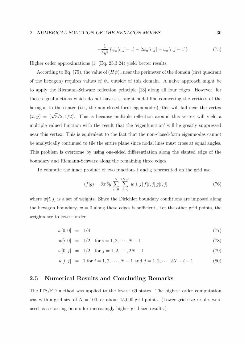
According to Eq. (75), the value of (Hψ)n near the perimeter of the domain (first quadrant
of the hexagon) requires values of ψn outside of this domain. A naive approach might be
to apply the Riemann-Schwarz reflection principle [13] along all four edges. However, for
those eigenfunctions which do not have a straight nodal line connecting the vertices of the
hexagon to the center (i.e., the non-closed-form eigenmodes), this will fail near the vertex
(x, y) = (√
3/2, 1/2). This is because multiple reflection around this vertex will yield a
multiple valued function with the result that the ‘eigenfunction’ will he greatly suppressed
near this vertex. This is equivalent to the fact that the non-closed-form eigenmodes cannot
be analytically continued to tile the entire plane since nodal lines must cross at equal angles.
This problem is overcome by using one-sided differentiation along the slanted edge of the
boundary and Riemann-Schwarz along the remaining three edges.
To compute the inner product of two functions f and g represented on the grid use
〈f |g〉 = δx δyN∑
i=0
2N−1∑
j=0
w[i, j] f [i, j] g[i, j] (76)
where w[i, j] is a set of weights. Since the Dirichlet boundary conditions are imposed along
the hexagon boundary, w = 0 along these edges is sufficient. For the other grid points, the
weights are to lowest order
w[0, 0] = 1/4 (77)
w[i, 0] = 1/2 for i = 1, 2, · · · , N − 1 (78)
w[0, j] = 1/2 for j = 1, 2, · · · , 2N − 1 (79)
w[i, j] = 1 for i = 1, 2, · · · , N − 1 and j = 1, 2, · · · , 2N − i− 1 (80)
2.5 Numerical Results and Concluding Remarks
The ITS/FD method was applied to the lowest 69 states. The highest order computation
was with a grid size of N = 100, or about 15,000 grid-points. (Lower grid-size results were
used as a starting points for increasingly higher grid-size results.)
2 NUMERICAL SOLUTION OF THE HEXAGON MODES 31
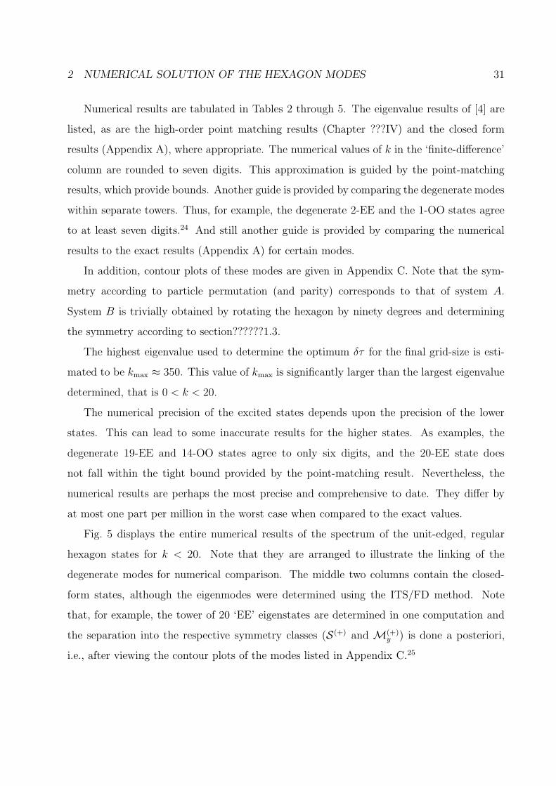
Numerical results are tabulated in Tables 2 through 5. The eigenvalue results of [4] are
listed, as are the high-order point matching results (Chapter ???IV) and the closed form
results (Appendix A), where appropriate. The numerical values of k in the ‘finite-difference’
column are rounded to seven digits. This approximation is guided by the point-matching
results, which provide bounds. Another guide is provided by comparing the degenerate modes
within separate towers. Thus, for example, the degenerate 2-EE and the 1-OO states agree
to at least seven digits.24 And still another guide is provided by comparing the numerical
results to the exact results (Appendix A) for certain modes.
In addition, contour plots of these modes are given in Appendix C. Note that the sym-
metry according to particle permutation (and parity) corresponds to that of system A.
System B is trivially obtained by rotating the hexagon by ninety degrees and determining
the symmetry according to section??????1.3.
The highest eigenvalue used to determine the optimum δτ for the final grid-size is esti-
mated to be kmax ≈ 350. This value of kmax is significantly larger than the largest eigenvalue
determined, that is 0 < k < 20.
The numerical precision of the excited states depends upon the precision of the lower
states. This can lead to some inaccurate results for the higher states. As examples, the
degenerate 19-EE and 14-OO states agree to only six digits, and the 20-EE state does
not fall within the tight bound provided by the point-matching result. Nevertheless, the
numerical results are perhaps the most precise and comprehensive to date. They differ by
at most one part per million in the worst case when compared to the exact values.
Fig. 5 displays the entire numerical results of the spectrum of the unit-edged, regular
hexagon states for k < 20. Note that they are arranged to illustrate the linking of the
degenerate modes for numerical comparison. The middle two columns contain the closed-
form states, although the eigenmodes were determined using the ITS/FD method. Note
that, for example, the tower of 20 ‘EE’ eigenstates are determined in one computation and
the separation into the respective symmetry classes (S (+) and M(+)y ) is done a posteriori,
i.e., after viewing the contour plots of the modes listed in Appendix C.25

2 NUMERICAL SOLUTION OF THE HEXAGON MODES 32
Table 2: Even-even (EE) hexagon eigenvalues. The first column lists the symmetry accordingto permutation S3 and inversion i The finite-difference values of k are rounded to seven digits.For comparison, the Bauer-Reiss results of Ref. [4] and the bounded point-matching resultsof chapter ???IV are also listed.
Finite-difference Bauer-Reiss Point-Matching
i⊗ S3 mode k mode k mode k
S(+) 1-EE 2.674947 1 2.67495 1-(oee) 2.6749465 8022
M(+)y 2-EE 5.696653 5 5.69666
S(+) 3-EE 6.123018 6 6.12303 2-(oee) 6.1230 2111
M(+)y 4-EE 8.374984 12 8.37500
M(+)y 5-EE 9.355850 14 9.35586
S(+) 6-EE 9.489908 15 9.48994 3-(oee) 9.489 9288
S(+) 7-EE 10.99398 19 10.99401 4-(oee) 10.9939 8652
M(+)y 8-EE 12.06157
M(+)y 9-EE 12.86524
S(+) 10-EE 12.99310 5-(oee) 12.993 1206
M(+)y 11-EE 13.68729
S(+) 12-EE 14.83148 6-(oee) 14.831 5240
M(+)y 13-EE 15.35073
M(+)y 14-EE 16.23500
S(+) 15-EE 16.54452 7-(oee) 16.544 5548
M(+)y 16-EE 16.57898
M(+)y 17-EE 17.73468
S(+) 18-EE 17.97028 8-(oee) 17.970 3513
M(+)y 19-EE 18.88865
S(+) 20-EE 18.99836 9-(oee) 18.99838 5901

2 NUMERICAL SOLUTION OF THE HEXAGON MODES 33
Table 3: Odd-Odd (OO) hexagon eigenvalues. The first column lists the symmetry accordingto permutation S3 and inversion i. The finite-difference values of k are rounded to sevendigits. For comparison, the Bauer-Reiss results of Ref [BR-78] and equilateral triangle closed-
form results (Appendix A, k = 4π√λ/3) are also listed.
Finite-difference Bauer-Reiss Closed-form
i⊗ S3 mode k mode k λ k
M(+)x 1-OO 5.696653 4 5.69666
M(+)x 2-OO 8.374984 11 8.37500
M(+)x 3-OO 9.355850 13 9.35586
A(+) 4-OO 11.08250 21 11.08252 7 11.08250
M(+)x 5-OO 12.06157
M(+)x 6-OO 12.86524
M(+)x 7-OO 13.68729
A(+) 8-OO 15.10289 13 15.10290
M(+)x 9-OO 15.35073
M(+)x 10-OO 16.23500
M(+)x 11-OO 16.57900
M(+)x 12-OO 17.73469
A(+) 13-OO 18.25849 19 18.25851
M(+)x 14-OO 18.88862
A(+) 15-OO 19.19543 21 19.19545

2 NUMERICAL SOLUTION OF THE HEXAGON MODES 34
24Of course, they could both be wrong by the same amount.25The symmetry according to particle permutation and spatial inversion of systems A and B are listed
under the figure and may be helpful in identifying the system B symmetry of the contour plots.

2 NUMERICAL SOLUTION OF THE HEXAGON MODES 35
Table 4: Odd-even (OE) hexagon eigenvalues. The first column lists the symmetry accordingto permutation S3 and inversion i. The finite-difference values of k are rounded to sevendigits. For comparison, the Bauer-Reiss results of Ref. [BR-78] and equilateral triangle
closed-form results (Appendix A, k = 4π√λ/3) are also listed.
Finite-difference Bauer-Reiss Closed-form
i⊗ S3 mode k mode k λ k
M(−)x 1-OE 4.258131 2 4.25814
A(−) 2-OE 7.255197 8 7.25520 3 7.255197
M(−)x 3-OE 7.752748 9 7.75276
M(−)x 4-OE 9.712134 17 9.71215
A(−) 5-OE 11.08250 20 11.08250 7 11.08250
M(−)x 6-OE 11.18237
M(−)x 7-OE 12.35573
M(−)x 8-OE 13.54386
A(−) 9-OE 14.51039 12 14.51039
M(−)x 10-OE 14.74507
A(−) 11-OE 15.10289 13 15.10290
M(−)x 12-OE 16.31809
M(−)x 13-OE 16.81988
M(−)x 14-OE 17.68348
A(−) 15-OE 18.25849 19 18.25851
M(−)x 16-OE 18.33968
A(−) 17-OE 19.19543 21 19.19545

2 NUMERICAL SOLUTION OF THE HEXAGON MODES 36
Table 5: Even-odd (EO) hexagon eigenvalues. The first column lists the symmetry accordingto permutation S3 and inversion i. The finite-difference values of k are rounded to sevendigits. For comparison, the Bauer-Reiss results of Ref. [BR-78] and the bounded point-matching results of chapter??? IV are also listed.
Finite-difference Bauer-Reiss Point-Matching
i⊗ S3 mode k mode k mode k
M(−)y 1-EO 4.258131 3 4.25814
S(−) 2-EO 6.901403 7 6.90142 1-(ooe) 6.90140 3523
M(−)y 3-EO 7.752748 10 7.75276
M(−)y 4-EO 9.712133 16 9.71215
S(−) 5-EO 10.50498 18 10.50503 2-(ooe) 10.5049 9753
M(−)y 6-EO 11.18237
M(−)y 7-EO 12.35573
M(−)y 8-EO 13.54386
S(−) 9-EO 13.76639 3-(ooe) 13.766 4331
M(−)y 10-EO 14.74507
S(−) 11-EO 14.98915 4-(ooe) 14.9891 5845
M(−)y 12-EO 16.31809
M(−)y 13-EO 16.81987
S(−) 14-EO 17.22765 5-(ooe) 17.227 7133
M(−)y 15-EO 17.68347
M(−)y 16-EO 18.33971
S(−) 17-EO 19.06539 6-(ooe) 19.065 4433

2 NUMERICAL SOLUTION OF THE HEXAGON MODES 37
Figure 5: The spectrum of the unit-edged, regular hexagonal region with Dirichlet boundaryconditions. The symmetry of the systems A and B is listed at the bottom. Note that thelevels are arranged so that degenerate levels line up for easy comparison. The middle twocolumns correspond to closed-form modes.

3 THE WAVEGUIDE PROBLEM 38
3 THE WAVEGUIDE PROBLEM
3.1 Preliminaries
The closed-form eigenmodes26 of the equilateral triangle were first published by Lame [16]
in 1852. Properties and derivations of these closed-form eigenmodes are discussed in the
literature in many places. Modern applications include the electromagnetic waveguide prob-
lem {[29], [21], [25], [39]} and several quantum-mechanical problems {[31], [10], [9], [8], [20],
[35]}. In addition, the eigenvalue problem is treated in Refs. {[22], [26], [13]}. Appendix A
contains a summary of the closed-form modes.
This report examines the relationship between eigenmodes of waveguides with various
cross sections which are constructed by piecing together identical 30◦-60◦-90◦ triangles, as
shown in Fig. 6 [25]. For simplicity, the guides are assumed to be uniform and perfectly
conducting. The shapes include (I) the 30◦-60◦-90◦ triangle, (II) the equilateral triangle,
(111) the kite quadrilateral, (IV) the 30◦-120◦-30◦ triangle, and (V) the rhombus. These
cross sections were chosen because many of their modes are expressible in closed form and
because this set includes all possible cross sections with a 30◦-60◦-90◦ triangular, fundamental
region with simple edge conditions.27
In the next chapter, the point-matching method is described and numerical estimates
of the eigenmodes are presented. One utility and selling point of this method is that a
relatively large number of eigenmodes are obtained with a modest amount of work. In
addition, a small number of parameters are required to represent the eigenfunctions. Using
five or six parameters, 53 distinct eigenfunctions – accurate to at least three digits in the
eigenvalue – are reported. Some additional benefits are that, with the chosen representation
of the approximate eigenfunctions, the modes may be easily compared to the modes within
a circular cross section; and unlike other methods, such as finite elements [4], (for example),
the numerical accuracy of each mode does not depend upon the accuracy of lower modes.
It was discovered that the point-matching method, when applied to the present problem,
26By ’closed-form’, it is meant that each eigenfunction may be written as a finite sum of plane waves.27The fundamental region of the regular hexagon is also a 30◦-60◦-90◦ triangle since its symmetry group
is of order twelve; however, the edge conditions are generally more complicated.

3 THE WAVEGUIDE PROBLEM 39
Figure 6: The waveguide cross-sections formed by piecing together identical 30◦-60◦-90◦
triangles. The dashed lines indicate the symmetry axes. These are the only shapes forwhich complete sets of eigenmodes may be obtained using the eight symmetry classes of the30◦-60◦-90◦ triangle.

3 THE WAVEGUIDE PROBLEM 40
may provide arbitrarily tight upper and lower bounds to each eigenvalue. Since bracketing
eigenvalues is in general rather difficult, this is a very important result. There do exist
other bracketing methods (which may use the point-matching results) {[15], [24], [14], [13]};however, they appear to provide much wider bounds for equivalent amounts of work.
3.2 The Eigenvalue Problem
The waveguide modes are determined [11] by solving the eigenvalue problem[∂2
∂x2+
∂2
∂y2+ k2
]ψ(x, y) = 0 (81)
inside the respective cross section and subject to the appropriate boundary conditions. The
eigenparameter k is the cutoff wavenumber. The Dirichlet and Neumann boundary con-
ditions divide the modes into two types – namely, the transverse magnetic (TM) and the
transverse electric (TE) modes, respectively. Let S be the boundary of the cross section;
then the boundary conditions are
TM : ψ|S = 0 (82)
TE : ∂ψ/∂n|S = 0 (83)
where ∂/∂n|S is the normal derivative on S. Note that by re-scaling the coordinates, results
may be extended; thus under the transformation (x, y)→ (ax, ay) the cutoff wavenumber k
becomes k/a.
The Riemann-Schwarz reflection principle [13] (for example) may be used to analytically
continue a harmonic function u(x, y) through a straight-line bounding edge as long as the
function remains single valued. Let x = 0 be such a line; then this line is even or odd
according to whether u(−x, y) = ±u(x, y). For any convex polygon cross section, and in
particular those of Fig. 6, the bounding edges of the TE and TM modes are respectively
even and odd.
3.3 Geometrical Classification Scheme
The geometrical symmetry of the cross section provides a classification scheme for the eigen-
modes. The cross sections of Fig. 6 have symmetry axes indicated by the dashed lines defined

3 THE WAVEGUIDE PROBLEM 41
by the joining of the 30◦-60◦-90◦ triangles. Every mode may be classified as either even or
odd with respect to reflection through these axes. This divides the modes into separate
orthogonal, symmetry classes, each of which contains an infinite set of modes such that
0 < λ0 ≤ λ1 ≤ λ2 ≤ · · · (84)
where λ = k2. There are no accumulations in the eigenvalue [27]. However, accidental
degeneracies of the closed-form modes may become arbitrarily large {[31], [26]}.Using the Riemann-Schwarz reflection principle, the complete sets of modes for each
symmetry class, boundary condition, and cross section of Fig. 6 may be constructed from
the complete sets of eigenmodes inside the 30◦-60◦-90◦ triangle with the eight possible edge
conditions.28 The set of cross-sections of Fig. 6 contains all of the possible domains for which
this method works. The 30◦-60◦-90◦ triangle is called the fundamental region since it is the
smallest region from which all of the modes may be obtained using reflections. The size and
orientation of the fundamental region is shown in Fig. 7.
Denote each set of edge conditions with an ordered triple of letters out of ’e’ (for even)
and ’o’ (for odd) to represent the symmetry of the edges A, B, and C respectively. For
example, if A, B, and C are even, odd, and even, respectively, then use (eoe) to denote
the edge conditions. If one or more edge conditions are arbitrary or unspecified, use an
asterisk as a place holder; thus, for example, all modes with odd edge B and even edge C
are symbolized using (*oe). The eight symmetry classes are illustrated in Fig. 8.
The classification scheme is summarized in Table 6 and makes explicit the relation be-
tween the eight symmetry classes of the fundamental region and the TE and TM modes of
the cross sections of Fig. 6. Note that the edge condition of the hypotenuse C determines
the boundary condition of the rhombus, and use, for example, ’eo-TE’, to indicate that the
shorter and longer symmetry axes are, respectively, even and odd for a TE mode.
In passing, we note that sets of modes with more complicated cross sections may be
obtained using the reflection principle. For example, each of the fundamental region eigen-
modes with an even (odd) leg A may be repeatedly reflected through legs B and C to obtain
sets of regular hexagon TE (TM) modes {[29], [4], [35]}. However, not all hexagon modes
28The 30◦-60◦-90◦ triangle TE (TM) modes correspond to all even (odd) edges.

3 THE WAVEGUIDE PROBLEM 42
Figure 7: Size and orientation of the 30◦-60◦-90◦ triangular, fundamental region. Both theCartesian coordinates (x, y) and Polar coordinates (r, θ) are shown. The edge lengths areLA = 1/2, LB =
√3/2, and LC = 1.
Table 6: Classification scheme of modes with the five cross sections shown in Fig. 6. Notethat the first four symmetry classes correspond to those closed form-modes of the equilateraltriangle. Thus, for example, only the even-TE and odd-TM modes of the kite quadrilateralshape (III) are expressible in closed form.
(ABC) I II III IV V
(eee) TE e-TE e-TE e-TE ee-TE
(eoe) o-TE eo-TE
(oeo) e-TM oe-TM
(ooo) TM o-TM o-TM o-TM oo-TM
(eeo) o-TE ee-TM
(oee) o-TE oe-TE
(eoo) e-TM eo-TM
(ooe) e-TM oo-TE

3 THE WAVEGUIDE PROBLEM 43
Figure 8: This diagram illustrates the eight symmetry classes of the 30◦-60◦-90◦ triangle.The even (Neumann) and odd (Dirichlet) edges are indicated using dashed and solid linesrespectively.
3 THE WAVEGUIDE PROBLEM 44
are obtained in this way. In fact only those TE (edge-A even) or TM (edge-A odd) hexagon
modes with three even (edge-C even) or three odd (edge-C odd) lines connecting opposite
pairs of vertices and three even (edge-B even) or three odd (edge-B odd) lines connecting the
centers of opposite edges are obtained using the 30◦-60◦-90◦, triangle modes with the eight
possible edge conditions. Contour plots of the lowest 69 TM hexagon modes are displayed
in appendix C.
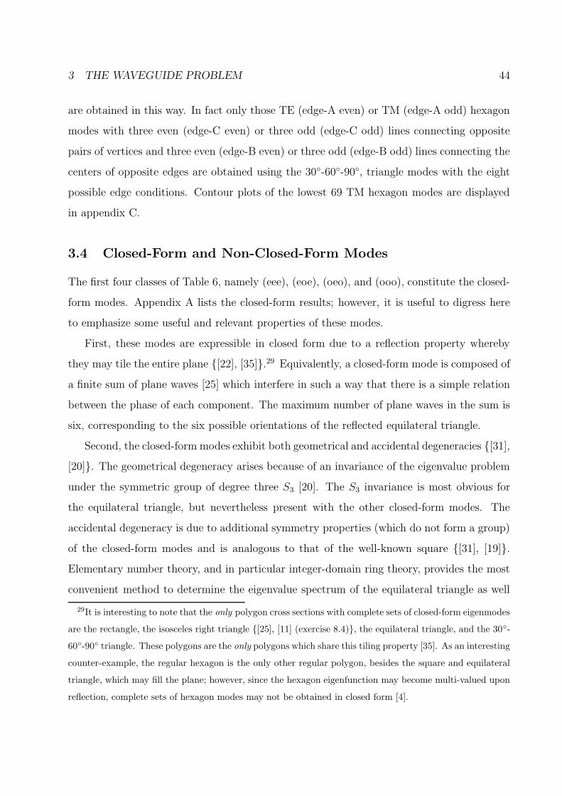
3.4 Closed-Form and Non-Closed-Form Modes
The first four classes of Table 6, namely (eee), (eoe), (oeo), and (ooo), constitute the closed-
form modes. Appendix A lists the closed-form results; however, it is useful to digress here
to emphasize some useful and relevant properties of these modes.
First, these modes are expressible in closed form due to a reflection property whereby
they may tile the entire plane {[22], [35]}.29 Equivalently, a closed-form mode is composed of
a finite sum of plane waves [25] which interfere in such a way that there is a simple relation
between the phase of each component. The maximum number of plane waves in the sum is
six, corresponding to the six possible orientations of the reflected equilateral triangle.
Second, the closed-form modes exhibit both geometrical and accidental degeneracies {[31],
[20]}. The geometrical degeneracy arises because of an invariance of the eigenvalue problem
under the symmetric group of degree three S3 [20]. The S3 invariance is most obvious for
the equilateral triangle, but nevertheless present with the other closed-form modes. The
accidental degeneracy is due to additional symmetry properties (which do not form a group)
of the closed-form modes and is analogous to that of the well-known square {[31], [19]}.Elementary number theory, and in particular integer-domain ring theory, provides the most
convenient method to determine the eigenvalue spectrum of the equilateral triangle as well
29It is interesting to note that the only polygon cross sections with complete sets of closed-form eigenmodes
are the rectangle, the isosceles right triangle {[25], [11] (exercise 8.4)}, the equilateral triangle, and the 30◦-
60◦-90◦ triangle. These polygons are the only polygons which share this tiling property [35]. As an interesting
counter-example, the regular hexagon is the only other regular polygon, besides the square and equilateral
triangle, which may fill the plane; however, since the hexagon eigenfunction may become multi-valued upon
reflection, complete sets of hexagon modes may not be obtained in closed form [4].

3 THE WAVEGUIDE PROBLEM 45
as the square {[6], [31], [26], [13], [20]}.Finally, a practical result is that the first accidental degeneracy within a given symmetry
class occurs for a relatively large cutoff wavenumber. Specifically, accidental degeneracy is
absent in the lowest 19 (eee), 15 (eoe), 24 (oeo), and 19 (ooo) eigenvalues. However, the first
accidental degeneracy is between the second (eee) mode and the lowest (oeo) mode.
The last four classes of Table 6, namely (eeo), (oee), (eoo), and (ooe), constitute the
non-closed-form modes. Since these modes are not invariant under any symmetry group
with an irreducible representation of dimension greater than one, geometrical degeneracies
are impossible. Also, since these modes may not tile the entire plane, and do not have the
same high symmetry properties as the closed-form modes, any degeneracy in these modes is
very unlikely and probably absent.
In the next chapter, a great effort is made to estimate the eigenvalues and eigenfunc-
tions of the 30◦-60◦-90◦ triangular domain. This is done by expanding the eigenfunction
in a Fourier-Bessel series and using the point-matching method to estimate the expansion
coefficients and cutoff wavenumbers.
3.5 Concluding Remarks
In this chapter, the waveguide modes within guides of several cross-sectional shapes formed
by piecing together 30◦-60◦-90◦ triangles are examined. They are divided up into eight
symmetry classes, based on simple edge conditions along the edges of the 30◦-60◦-90◦ triangle.
Four of the eight symmetry classes are expressible in closed form and only these modes may
be analytically continued to tile the entire plane.
Our next step is to determine precisely the lowest eigenvalues (i.e., cutoff wavenumbers)
and eigenfunctions of the eight symmetry classes of the 30◦-60◦-90◦ triangle, at least for
those non-closed-form modes. Once this is done, practical applications which require these
lowest may be made.
4 THE POINT-MATCHING METHOD 46
4 THE POINT-MATCHING METHOD
4.1 Preliminaries
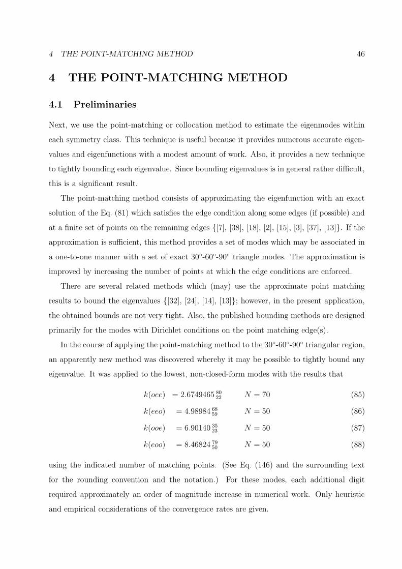
Next, we use the point-matching or collocation method to estimate the eigenmodes within
each symmetry class. This technique is useful because it provides numerous accurate eigen-
values and eigenfunctions with a modest amount of work. Also, it provides a new technique
to tightly bounding each eigenvalue. Since bounding eigenvalues is in general rather difficult,
this is a significant result.
The point-matching method consists of approximating the eigenfunction with an exact
solution of the Eq. (81) which satisfies the edge condition along some edges (if possible) and
at a finite set of points on the remaining edges {[7], [38], [18], [2], [15], [3], [37], [13]}. If the
approximation is sufficient, this method provides a set of modes which may be associated in
a one-to-one manner with a set of exact 30◦-60◦-90◦ triangle modes. The approximation is
improved by increasing the number of points at which the edge conditions are enforced.
There are several related methods which (may) use the approximate point matching
results to bound the eigenvalues {[32], [24], [14], [13]}; however, in the present application,
the obtained bounds are not very tight. Also, the published bounding methods are designed
primarily for the modes with Dirichlet conditions on the point matching edge(s).
In the course of applying the point-matching method to the 30◦-60◦-90◦ triangular region,
an apparently new method was discovered whereby it may be possible to tightly bound any
eigenvalue. It was applied to the lowest, non-closed-form modes with the results that
k(oee) = 2.6749465 8022 N = 70 (85)
k(eeo) = 4.98984 6859 N = 50 (86)
k(ooe) = 6.90140 3523 N = 50 (87)
k(eoo) = 8.46824 7950 N = 50 (88)
using the indicated number of matching points. (See Eq. (146) and the surrounding text
for the rounding convention and the notation.) For these modes, each additional digit
required approximately an order of magnitude increase in numerical work. Only heuristic
and empirical considerations of the convergence rates are given.

4 THE POINT-MATCHING METHOD 47
To compare the above results with other results, I obtained ‘unbounded’ values of k(oee) =
2.67494652 and k(ooe) = 6.9014027, using finite elements. Ref. [4] cites k(oee) = 2.67495
and k(ooe) = 6.90142, which are obtained using Richardson extrapolation of low-order finite-
difference results. For the lowest (eeo) mode, Ref. [32] gives a bound of 4.988 < k(eeo) < 4.998,
using an affine transformation method. It may be added that the results of Eqs. (85)-(88)
are probably the world’s best for this problem to date.
The closed-form modes have a considerably faster rate of convergence – by many orders
of magnitude – than their non-closed-form cousins. This is true despite the facts that the
Bessel functions represent ‘circular waves,’ and both closed-form and non-closed-form modes
are treated equivalently.30 (See the comment made in Ref. [32] (Sec. 7) regarding ability to
tightly bound eigenvalues in the rhombus.)
The lowest closed-form (eee) mode was bounded using only two through five matching
points with the results
k(eee) =
4.188 8877 N = 2
4.188 790 204 8948 N = 3
4.188 790 204 786 39 1208 N = 4
4.188 790 204 786 390 984 616 8 7631 N = 5
(89)
(See Eq. (146) and the surrounding text for the rounding convention and the notation.)
These consistently bound the exact value of
k(eee) =4π
3= 4.188 790 204 786 390 984 616 857 844 · · · (90)
thus verifying the new bounding method. Similar incredible results were obtained for several
of the other closed-form modes; however, they are not reported here. (An obtuse method of
30May this difference in convergence rates be used as a flag to identify yet undiscovered closed-form modes
of other geometries and dimensions? For example, are certain modes of the regular tetrahedron expressible
in closed form? This shape is interesting because (analogous to the equilateral triangle in two dimensions)
its modes may fill the space using reflections. See Refs. [8], [34], for a related problem. Another interesting
geometry is the regular dodecahedron since it can be related to the one-dimensional, quantum-mechanical
four-body problem with infinite square-wells. In particular, are the four-body, antisymmetric states (Dirichlet
modes in a pyramid with a pentagon base) expressible in closed-form?

4 THE POINT-MATCHING METHOD 48
tightly bounding π is thus obtained. This is vaguely analogous to the suggestion that the
point-matching and a bounding method may be used to bracket the zeros of certain Mathieu
functions [15].)
To begin, it is necessary to consider under what conditions the point matching method
is valid and reliable {[18], [2], [3], [37]}. For this reason, all details are given in the next
section.
4.2 Details of the Point-Matching Method
With the usual polar coordinates defined by
x = r cos(θ) and y = r sin(θ) (91)
Eq. (81) becomes [∂2
∂r2+
1
r
∂
∂r+
1
r2
∂2
∂θ2+ k2
]ψ(r, θ) = 0 (92)
An arbitrary, finite solution of Eq. (92) may be expanded in a Fourier-Bessel series,
ψ(k; r, θ) =∑
m
αmφm(k; r, θ) (93)
where the sum is over all non-negative integers, the αm are coefficients, and the basis func-
tions are either
φm(k; r, θ) = Nm Jm(kr) cos(mθ) (94)
or
φm(k; r, θ) = Nm Jm(kr) sin(mθ) (95)
depending on the edge-B conditions, i.e., the symmetry of the eigenfunction under θ → −θ or
(x, y)→ (x,−y). (These results are elementary and may be found in Ref. [33], for example.)
The normalization constant Nm is given below by Eq. (115), and Jm(x) is the Bessel function
of integral order m. For any fixed value of k 6= 0, the φm(k; r, θ) form a complete set of finite
basis functions in the plane containing the origin. (If the origin is excluded, the Ym(x) must
be included to form a complete set of finite basis functions.)

4 THE POINT-MATCHING METHOD 49
The choice of basis functions φm is convenient since exact edge conditions along the longer
edges B and C may be trivially satisfied. In particular, using an obvious notation,
ψ(∗ee)(k; r, θ) =∑
m=0,6,12,···αmNm Jm(kr) cos(mθ) (96)
ψ(∗oo)(k; r, θ) =∑
m=6,12,18,···αmNm Jm(kr) sin(mθ) (97)
ψ(∗eo)(k; r, θ) =∑
m=3,9,15,···αmNm Jm(kr) cos(mθ) (98)
ψ(∗oe)(k; r, θ) =∑
m=3,9,15,···αmNm Jm(kr) sin(mθ) (99)
Note that the value of k in Eqs. (96)–(99) is not specified. To fix the value of k, the edge
condition along A must be enforced, which is done with either
ψ(o∗∗)∣∣∣A
= 0 or∂
∂xψ(e∗∗)
∣∣∣A
= 0 (100)
For a given set of edge conditions, there exists an infinite set of eigenfunctions and eigenval-
ues. Let ki for i = 1, 2, 3, · · ·; be the distinct cutoff wavenumbers where 0 < ki < ki+1. Also
let γi be the multiplicity of ki.31 Then, an exact eigenfunction may be written
ψ(s,i)(ki; r, θ) =∑
m
α(s,i)m φm(ki; r, θ) (101)
where s = 1, 2, · · · , γi labels degenerate eigenfunctions.
The point matching method provides a reliable and convenient method to determine the
numerical values of the k and α(s,i)m . In addition, the values of the coefficients permit a
simple physical interpretation of each eigenfunction by allowing a comparison between the
well-known circular modes and the 30◦-60◦-90◦ triangular modes.32 This comparison, in turn,
provides an elementary procedure to determine which terms of Eq. (101) are important. This
is good because, in practice, the sum (101) must be truncated above a certain number of
31This notation is more convenient than that of Eq. (84).32See Eq. (128) and the surrounding text for the interpretation. Briefly, α2
m is approximately equal to
the probability that the eigenfunction has a given ‘m-value’ within a hexagonal domain. Using the quantal
analog of a particle confined within a regular hexagonal domain (TM hexagon modes), this m-value is sort
of like an angular momentum (in units of h) of the particle. Of course, since the hexagon is not continuously
rotationally invariant, angular momentum is not a good quantum number and the interpretation need not
be taken literally.

4 THE POINT-MATCHING METHOD 50
terms. Before proceeding, it is necessary to examine some properties of the eigenfunctions
and basis functions.
One drawback and difficultly of the Fourier-Bessel series is that the basis functions are
orthonormalized in a circular region, not a polygonal region.33 For this reason, it is convenient
to define a 30◦ circular sector with an area equal to that of the 30◦-60◦-90◦ triangular,
fundamental region [4]. In addition, this circular region is oriented similar to the fundamental
region. More precisely, edges A, B, and C correspond respectively to the arc at r = R and
0 < θ < π/6, and the radii 0 < r < R at θ = 0 and θ = π/6. With equal-area regions (see
Eq. (113)), the radius of the sector is
R =
√3√
3
2π≈ 0.90939 (102)
Analogous to the eight symmetry classes of the 30◦-60◦-90◦ triangle, there exist eight sym-
metry classes of the 30◦ sector. The φm(k; r, θ) are normalized eigenfunctions within the
circular sector {[11], (Ex. 8.3)}. Imposing edge conditions on the arc at r = R gives the
possible values of k,
kmn ≡
jmn/R Dirichlet condition at r = R
j ′mn/R Neumann condition at r = R(103)
where jmn and j ′mn are the zeros (or roots) defined by Jm(jmn) = 0 and J′m(j ′mn) = 0, for
n = 1, 2, 3, · · · {[1], sec 9.5}. Since j ′0,1 = 0 is by convention the only vanishing zero, this
mode is trivial and may be ignored. The zeros interlace {[1], Eq. 9.5.2 and Table 9.5}according to
m ≤ j ′m,1 < jm,1 < j ′m,2 < jm,2 < j ′m,3 < · · · (104)
m < jm,1 < jm+1,1 < jm,2 < jm+1,2 < jm,3 < · · · (105)
m ≤ j ′m,1 < j ′m+1,1 < j ′m,2 < j ′m+1,2 < j ′m,3 < · · · (106)
where the equalities occur only with the unphysical j ′0,1 = 0. It is interesting to note that the
zeros of Jm and Jm+2 also interlace [36]; however, those of Jm and Jm+3 do not. In addition,
the only coincidences in the zeros occur with j ′0,n = j1,n−1 for n = 2, 3, 4, · · ·; this is because
J′0(z) = −J1(z) {[1], Eq. 9.5.1}.33Analogous to fitting a round peg (φm) into a polygonal hole (the edge conditions of ψ).

4 THE POINT-MATCHING METHOD 51
Imposing the edge conditions along the radii yield the normalized eigenfunctions in the
30◦ sector;
φ(∗ee)m (kmn; r, θ) = Nm Jm(kmnr) cos(mθ) where m = 0, 6, 12, · · · (107)
φ(∗oo)m (kkm; r, θ) = Nm Jm(kr) sin(mθ) where m = 6, 12, 18, · · · (108)
φ(∗eo)m (kmn; r, θ) = Nm Jm(kmnr) cos(mθ) where m = 3, 9, 15, · · · (109)
φ(∗oe)m (kmn; r, θ) = Nm Jm(kmnr) sin(mθ) where m = 3, 9, 15, · · · (110)
Compare these equations with Eqs. (96)–(99). The interlacing relations given by Eqs. (104)–
(106) prove that there is no degeneracy within any symmetry class of the 30◦ sector. How-
ever, a geometrical degeneracy exists between modes of different symmetry classes with
similar edge A conditions. Specifically, for m 6= 0, there exist pairs of degenerate modes
(φ(eee)m , φ(eoo)
m ); (φ(oee)m , φ(ooo)
m ); (φ(eeo)m , φ(eoe)
m ); and (φ(oeo)m , φ(ooe)
m ). These modes are obtained
from one another by rotation in the plane about the origin by π/2, which in effect trans-
forms the ‘sin’ into a ‘cos’ or visa-versa. There is no other degeneracy in these modes.34
Define the inner products of two well-behaved real functions, f and g,
(f |g) ≡ ∫ π/60 dθ∫ R0 r dr f(r, θ)g(r, θ) (30◦ sector) (111)
〈f |g〉 ≡ ∫√
3/20 dx
∫ x/√30 dy f(x, y)g(x, y) (30◦-60◦-90◦ triangle) (112)
The parentheses are used for the 30◦ circular sector (curved) while the angle brackets are
used for the 30◦-60◦-90◦ triangle (angled). The area of the sector and the fundamental region
is given by
A ≡ (1|1) =πR2
12= 〈1|1〉 =
√3
8(113)
This is used to fix the value of R given by Eq. (102).
The basis functions of a given symmetry class are partially orthonormalized in the 30◦
sector using
(φm(k)|φm′(k)) = A δmm′ (114)
34Recall that since the relevant m-values are multiples of three, the fact that j ′0,n = j1,n−1 (for n =
2, 3, 4, · · ·) does not lead to any accidental degeneracies. Of course, with a circular guide, the TE modes
J0(j′0,nr/R) are accidentally degenerate with the pairs of TM modes J1(j1,n−1r/R) sin(θ), cos(θ) {[11]
(Ex. 8.3)}

4 THE POINT-MATCHING METHOD 52
where δmm′ is the Kronecker delta function and k > 0 is (for now) arbitrary [15].35 Using
this normalization, the value of Nm depends only on the dimensionless parameter kR and is
determined using Eq. (114) with m = m′,
πR2
12= N 2
m ×[∫ π/6
0cos2(mθ) dθ
]×[k−2
∫ kR
0J2m(η) η dη
](115)
The integrals of Eq. (115) are elementary.36 Solving for Nm as a function of kR yields
Nm(kR) =
√2
σm
[J2m+1(kR) + J2
m(kR)−{
2m
kR
}Jm(kR) Jm+1(kR)
]−1/2
(116)
where σ0 = 2 and σm = 1 for m = 3, 6, 9, · · ·.The basis functions are approximately orthogonal in the fundamental region,
〈φm(k)|φm′(k)〉 = A [ δmm′ + εmm′(k)] ≈ A δmm′ (117)
where
εmm′(k) ≡[Nm(kR)Nm′(kR)
A k2
](118)
×∫ π/6
0dθ cos(mθ) cos(m′θ)
∫ k√
32 cos θ
kRη dη Jm(η) Jm′(η) (119)
is assumed to be small compared to unity. [In general, let f and g be well-behaved functions
in the plane such that (f |f) ≈ (g|g) ≈< f |f >≈< g|g >≈ A, then < f |g > −(f |g) ≡ Aε. If,
near r = R, there is either a node in f or g, or if f and g are relatively constant, then ε will
be small compared to unity. It is numerically verified that for k < 20, the |εmm′(k)| < 0.01.
For example, ε00(4.189) = −0.000218.]
With distinct value of k, the inner product of the basis functions becomes more compli-
cated. An exact treatment of the basis functions yields
(φm(kmn)|φm′(km′n′)) = Aδmm′δnn′ (120)
35The orthonormalization is partial in that only one value of k is considered. The more general expression
(φm(k)|φm′(k′)) is considered below.
36The Bessel function integral is∫ z
0 J2m(η)η dη = (z2/2)
[J′2m(z) + (1−m2/z2)J2
m(z)]{[33], Eq. 5.14.5},
where the derivative of the Bessel function is given by J′m(z) = mJm(z)/z − Jm+1(z) {[33], Eq. 5.2.6}.

4 THE POINT-MATCHING METHOD 53
where the kmn are given by Eq. (103). On the other hand, with arbitrary k 6= k′,
(φm(k)|φm′(k′)) = A δmm′Nm(kR)Nm(k′R)
R(k2 − k′2
)
(121)
× [ k′Jm(kR) J′m(k′R)− kJm(k′R) J′m(kR)] (122)
For kR and/or k′R not near a node of either Jm(η) or J′m(η), this expression is not necessarily
small. Note that in both of Eqs. (120) and (122), the δmm′ comes from the angular integration.
The coefficients in the expansion (101) may be determined using
(φm(ki)
∣∣∣ψ(s,i)(ki))
= Aα(s,i)m (123)
where ki is an ‘exact’ eigenvalue of the 30◦-60◦-90◦ triangle. However, note the approximation
⟨φm(ki)
∣∣∣ψ(s,i)⟩
= A[α(s,i)m +
∑
m′εmm′(k)α
(s,i)m′
]≈ Aα(s,i)
m (124)
The eigenfunctions within a given symmetry class are orthonormalized in the fundamental
region according to
⟨ψ(s,i)(ki)
∣∣∣ψ(t,j)(kj)⟩
= A δij δst =∑
mm′α(s,i)m α
(t,j)m′
⟨φm(ki)
∣∣∣φm′(kj)⟩
(125)
On the other hand, within the 30◦ sector the same two eigenfunctions satisfy
(ψ(s,i)(ki)
∣∣∣ψ(t,j)(kj))
=∑
mm′α(s,i)m α
(t,j)m′
(φm(ki)
∣∣∣φm′(kj))
(126)
[Editor’s note (2004): Eqs. (125) and (126) differ in the type of inner product, and the latter
is not proportional to δijδst.] Setting i = j (same eigenvalue), and using the approximation
of Eq. (117), Eqs. (125) and (126) yield the approximate relation for the coefficients
δst =∑
m
α(s,i)m α(t,i)
m +∑
mm′α(s,i)m εmm′(ki)α
(t,i)m′ ≈
∑
m
α(s,i)m α(t,i)
m (127)
Eqs. (124) and (127) suggest that α(s,i)m is approximately the amount of the basis function
φm(ki; r, θ) in the exact eigenfunction ψ(s,i)(ki; r, θ). The relative importance of each term is
determined by comparing each
P (s,i)m ≡
[α(s,i)m
]2(128)
in complete analogy with the quantum mechanical interpretation of the coefficients. (The
Pm are non-negative and approximately less than unity since∑m Pm ≈ 1). Although the
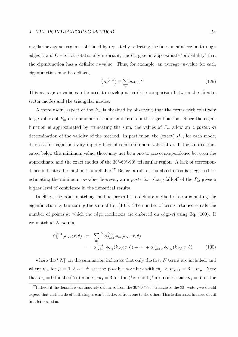
4 THE POINT-MATCHING METHOD 54
regular hexagonal region – obtained by repeatedly reflecting the fundamental region through
edges B and C – is not rotationally invariant, the Pm give an approximate ‘probability’ that
the eigenfunction has a definite m-value. Thus, for example, an average m-value for each
eigenfunction may be defined,⟨m(s,i)
⟩≡∑
m
mP (s,i)m (129)
This average m-value can be used to develop a heuristic comparison between the circular
sector modes and the triangular modes.
A more useful aspect of the Pm is obtained by observing that the terms with relatively
large values of Pm are dominant or important terms in the eigenfunction. Since the eigen-
function is approximated by truncating the sum, the values of Pm allow an a posteriori
determination of the validity of the method. In particular, the (exact) Pm, for each mode,
decrease in magnitude very rapidly beyond some minimum value of m. If the sum is trun-
cated below this minimum value, there may not be a one-to-one correspondence between the
approximate and the exact modes of the 30◦-60◦-90◦ triangular region. A lack of correspon-
dence indicates the method is unreliable.37 Below, a rule-of-thumb criterion is suggested for
estimating the minimum m-value; however, an a posteriori sharp fall-off of the Pm gives a
higher level of confidence in the numerical results.
In effect, the point-matching method prescribes a definite method of approximating the
eigenfunction by truncating the sum of Eq. (101). The number of terms retained equals the
number of points at which the edge conditions are enforced on edge-A using Eq. (100). If
we match at N points,
ψ(s,i)N (kN,i; r, θ) ≡
∑
m
[N ]α
(s,i)N,m φm(kN,i; r, θ)
= α(s,i)N,m1
φm1(kN,i; r, θ) + · · ·+ α(s,i)N,mN
φmN (kN,i; r, θ) (130)
where the ‘[N ]’ on the summation indicates that only the first N terms are included, and
where mµ for µ = 1, 2, · · · , N are the possible m-values with mµ < mµ+1 = 6 + mµ. Note
that m1 = 0 for the (*ee) modes, m1 = 3 for the (*eo) and (*oe) modes, and m1 = 6 for the
37Indeed, if the domain is continuously deformed from the 30◦-60◦-90◦ triangle to the 30◦ sector, we should
expect that each mode of both shapes can be followed from one to the other. This is discussed in more detail
in a later section.

4 THE POINT-MATCHING METHOD 55
(*oo) modes. Each ψ(s,i)N thus has N+1 parameters, namely, kN,i and the N coefficients α
(s,i)N,m.
Matching at N points yields N independent, constraint equations; thus, together with the
normalization, it is possible to determine values of the N + 1 parameters for each of the
eigenfunctions. Implicit are the assumptions that the set of matching points are distinct and
exclude those points where the edge conditions are satisfied trivially – as may occur at the
end-points of A.
In the limit that the matching points become infinitely dense along the edge A, the
approximate values must approach the exact values. In particular, if δy is the maximum
separation between adjacent matching points, then
limδy→0
kN,i = ki and limδy→0
α(s,i)N,m = α(s,i)
m (131)
which imply that
limδy→0
ψ(s,i)N = ψ(s,i) (132)
These are valid because the edge conditions are satisfied exactly in the limit that δy = 0. Note
that if the matching points are (approximately) equally spaced along A, then δy ≈ 1/(2N),
and the above limits are equivalent to the N →∞ limit. For convergence to the ‘exact’
value, necessary condition is that δy → 0 [corrected 2004] which requires that N →∞.38
Next, a general rule-of-thumb criterion is given for estimating the minimum number
of terms necessary for a reliable truncation. To be definite, consider the application to
the modes with cutoff wavenumbers between zero and some maximum value, 0 < k < kmax.
These results, however elementary, appear to be new.
First consider the (o**) modes. Ignoring the possibility of cancellation between terms,
the dominant terms, i.e., those with large Pm, heuristically should have a node near r = R,
i.e. near edge A. These nodes are governed by the nodes of the Bessel functions. Keeping in
mind interlacing relation Eq. (105), it is obvious that the truncation must not occur below
order m where
kmaxR < jm,1 (odd edge A) (133)
38The N → ∞ limit does not imply that δy → 0. For example, exclusion of the points between y = 0
and y = y0, where 0 < y0 < 1/2, prevents δy from becoming smaller than y0 no matter how large N may
become.

4 THE POINT-MATCHING METHOD 56
The Bessel functions of order greater than m do not support nodes at values of r < R, and
they serve to refine the eigenfunctions near the edge A. On the other hand, the dominant
terms govern the behavior of the eigenfunctions within the interior region.
The arguments for the (e**) modes are similar. Specifically, the dominant terms should
have an node in the derivative (with respect to r) near r = R with the result that
kmaxR < j ′m,1 (even edge A) (134)
where m is again the highest order.
If the number of terms in the expansion is sufficient, a contour along which the edge A
conditions are satisfied must pass continuously from edge B, through the matching points,
to edge C. This is a more difficult criterion to enforce, yet it must be satisfied for any
approximation to be valid.
In the numerical analysis, the normalization given by Eq. (127) is inconvenient because it
involves approximations. Therefore – instead of determining the εmm′ of Eq. (119) – impose
1 ≡∑
m
[N ] [α
(s,i)N,m
]2and α
(s,i)N,m1
≥ 0 (135)
for each of the approximate eigenfunctions ψ(s,i)N given by Eq. (130). The general meaning of
the coefficients is not lost; instead, the normalization of the eigenfunction is slightly modified.
However, this modification does not affect the values of kN,i.
To illustrate the practical technique used in this project for the (o**) modes, consider an
approximate eigenfunction given by an abbreviated version of Eq. (130)
ψN(k; η) = αm1φm1(k; η) + αm2φm2(k; η) + · · ·+ αmNφmN (k; η) (136)
where η = (r, θ) and k are (for now) arbitrary. Let ηµ (for µ = 1, 2, · · · , N) denote the
N matching points on edge A. For simplicity assume that 0 ≤ yµ < yµ+1 ≤ 1/2 where
yµ = rµ sin(θµ) and xµ =√
3/2. Thus, the N independent constraints are ψN (k; ηµ) = 0.
For each non-trivial eigen-solution, the determinant must vanish,
∆N(k; {η}) ≡
∣∣∣∣∣∣∣∣∣∣∣∣∣∣
φm1(k; η1) φm2(k; η1) · · · φmN (k; η1)
φm1(k; η2) φm2(k; η2) · · · φmN (k; η2)...
.... . .
...
φm1(k; ηN) φm2(k; ηN) · · · φmN (k; ηN)
∣∣∣∣∣∣∣∣∣∣∣∣∣∣
= 0 (137)

4 THE POINT-MATCHING METHOD 57
This function ∆N (k; {η}) depends upon the number of matching points N , the distribution
of these points symbolized by {η}, and the eigenparameter k. Restricting the search to
values of k such that 0 < k < kmax < jmN ,1/R, the zeros of ∆N (k; {η}) are determined and
identified with the kN,i. After the kN,i are found, the coefficients α(s,i)N,m are determined subject
to Eq. (135). It is estimated numerically that a small induced error k → k ± δk, changes the
coefficients by αm → αm ± δαm where |δαm| < |δk|.The procedure is similar for the (e**) modes except that the constraints are ∂ψN (k; ηµ)/∂x = 0
and the values of k are limited by 0 < k < kmax < j ′mN ,1/R. It may be added that the com-
putation of the (e**) modes is a bit more involved because of the derivatives.
To speed up numerical computations for relatively large values of N , the matrix elements
of ∆N(k; {η}) were expanded in second or third order Taylor series about an estimate of
the eigenvalue κ ≈ kN . An improved value of κ′ ≈ kN was then determined. By repeating
this procedure and expanding about κ′, it was verified that this expansion method converges
very quickly, and in particular well within the reported precision.
Also, accidental degeneracies (which are possible with the closed-form triangle modes
as pointed out in Appendix A) are not encountered. This may be anticipated since (the
arbitrary value of) kmax = 20 is considerably smaller than the lowest accidental degeneracy
at k = 4π√
49/3 ≈ 29.3215. This is fortunate since an accidental degeneracy will result
(approximately) in a double root of ∆N (k; {η}). More effort must be made in examining the
behavior of the solutions in such a case.
4.3 Low-Order Point-Matching Results
Low order computations were performed for values of k from zero to twenty for all of the
symmetry classes. Each of the eigenvalues may be compared to exact values obtained using
higher order computations (done in a later section) or other methods. However, in this
section it is demonstrated that with a modest amount of numerical work, a relatively large
number of modes may be determined with a precision of three or more digits.
For simplicity, the N point-matching coordinates were chosen such that the subtended

4 THE POINT-MATCHING METHOD 58
angle between successive points is equal; namely,
θµ =π
6N
(µ− 1
2
)(138)
rµ =
√3/2
cos(θµ)(139)
where µ = 1, 2, . . . , N . This set of matching points satisfies the necessary condition that the
maximum distance between adjacent points δy → 0 as N →∞. The endpoints of edge A
are excluded because in some cases the edge conditions are trivially satisfied at these points.
This choice of distribution is not optimal and rather arbitrary. Any attempt to bound the
eigenvalues using the present computations is not made here.
For kmax = 20, Eqs. (133) and (134) yield m(A odd) = 13.1 and m(A even) = 16.1 re-
spectively. All computations included m-values of at least m = 18 which is the smallest
multiple of three greater than 16. The results are listed in Tables 7 through 14. Selected
values of N were four or five. Since the closed-form modes appear to converge more quickly,
N = 4 seemed very sufficient. In addition, the ‘odd-edge-A’ non-closed-form modes were
slightly easier to compute than the ‘even-edge-A’ non-closed-form modes; therefore, a larger
value of N (equal to five) was used.39
The 30◦ sector modes are given by Eqs. (107)–(110). The last two columns of Tables 7
through 14 list the values of (m,n) and kmn. given by Eq. (103). These are simply ordered
according to the values of kmn. The insight gained by comparing these modes is that the
correspondence between the modes is remarkable. Indeed, at least for the lowest modes, the
eigenvalues of both shapes agree to within several percent and the m-value of the dominant
term corresponds to the m-value of the circular mode. For example, the 4-(oee) mode has an
eigenvalue k = 10.9948 and a dominant coefficient α6 = 0.9265; whereas the corresponding
circular mode (m,n) = (6, 1) has k6,1 = 10.9261. The agreement gets worse as the eigenvalue
increases in value. I return to this in the next section.
One important observation is the a posteriori fact that enough terms were included in
the truncated eigenfunction. This can be seen from the one-to-one correspondence between
the circular modes and the triangular modes. Also, the Pm = α2m (for each mode) decreases
39In a later section, high-order computations of the non-closed-form modes are made, therefore, the present
limitations are not severe.
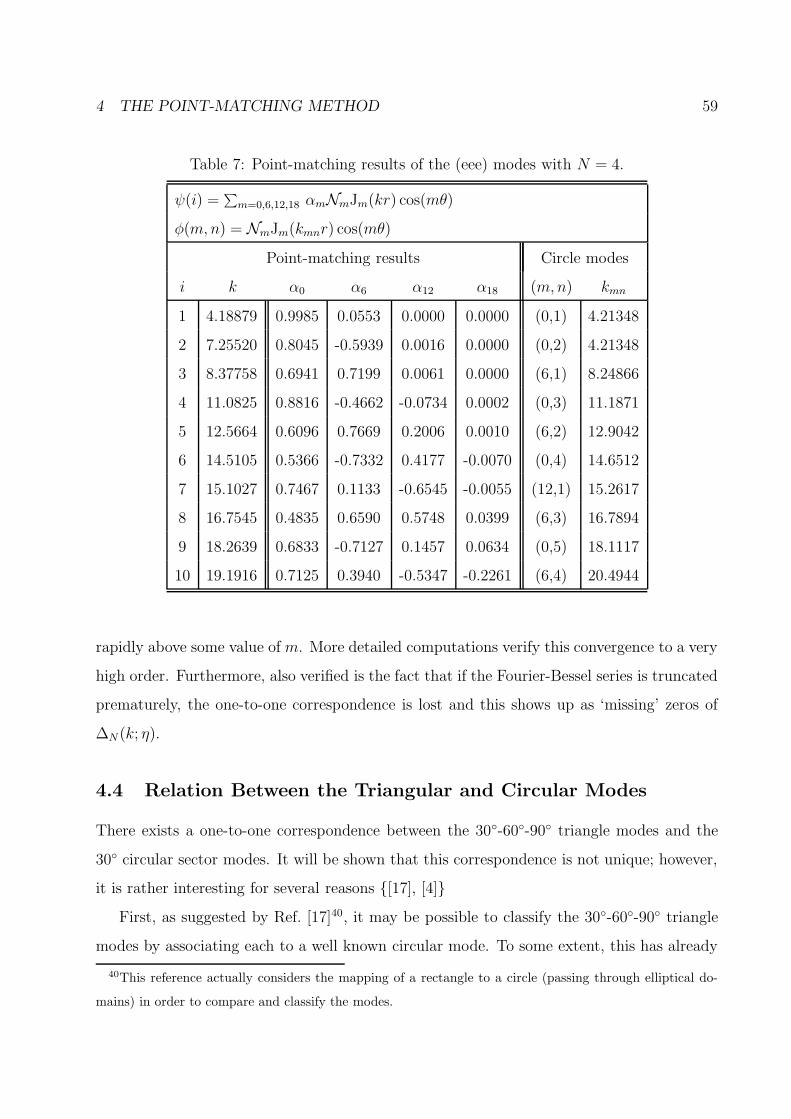
4 THE POINT-MATCHING METHOD 59
Table 7: Point-matching results of the (eee) modes with N = 4.
ψ(i) =∑m=0,6,12,18 αmNmJm(kr) cos(mθ)
φ(m,n) = NmJm(kmnr) cos(mθ)
Point-matching results Circle modes
i k α0 α6 α12 α18 (m,n) kmn
1 4.18879 0.9985 0.0553 0.0000 0.0000 (0,1) 4.21348
2 7.25520 0.8045 -0.5939 0.0016 0.0000 (0,2) 4.21348
3 8.37758 0.6941 0.7199 0.0061 0.0000 (6,1) 8.24866
4 11.0825 0.8816 -0.4662 -0.0734 0.0002 (0,3) 11.1871
5 12.5664 0.6096 0.7669 0.2006 0.0010 (6,2) 12.9042
6 14.5105 0.5366 -0.7332 0.4177 -0.0070 (0,4) 14.6512
7 15.1027 0.7467 0.1133 -0.6545 -0.0055 (12,1) 15.2617
8 16.7545 0.4835 0.6590 0.5748 0.0399 (6,3) 16.7894
9 18.2639 0.6833 -0.7127 0.1457 0.0634 (0,5) 18.1117
10 19.1916 0.7125 0.3940 -0.5347 -0.2261 (6,4) 20.4944
rapidly above some value of m. More detailed computations verify this convergence to a very
high order. Furthermore, also verified is the fact that if the Fourier-Bessel series is truncated
prematurely, the one-to-one correspondence is lost and this shows up as ‘missing’ zeros of
∆N (k; η).
4.4 Relation Between the Triangular and Circular Modes
There exists a one-to-one correspondence between the 30◦-60◦-90◦ triangle modes and the
30◦ circular sector modes. It will be shown that this correspondence is not unique; however,
it is rather interesting for several reasons {[17], [4]}First, as suggested by Ref. [17]40, it may be possible to classify the 30◦-60◦-90◦ triangle
modes by associating each to a well known circular mode. To some extent, this has already
40This reference actually considers the mapping of a rectangle to a circle (passing through elliptical do-
mains) in order to compare and classify the modes.

4 THE POINT-MATCHING METHOD 60
Table 8: Point-matching results of the (eoe) modes with N = 4.
ψ(i) =∑m=3,9,15,21 αmNmJm(kr) sin(mθ)
φ(m,n) = NmJm(kmnr) sin(mθ)
Point-matching results Circle modes
i k α3 α9 α15 α21 (m,n) kmn
1 4.18879 1.0000 0.0008 0.0000 0.0000 (3,1) 4.61978
2 8.37758 0.9908 0.1351 0.0002 0.0000 (3,2) 8.81384
3 11.0825 0.6795 -0.7336 0.0021 0.0000 (9,1) 11.7787
4 12.5664 0.7720 0.6354 -0.0189 0.0000 (3,3) 12.4764
5 15.1029 0.8180 -0.5542 -0.1539 0.0004 (3,4) 16.0391
6 16.7553 0.7235 0.6419 0.2540 0.0034 (9,2) 16.8099
7 18.2586 0.3172 -0.7706 0.5526 -0.0110 (15,1) 18.7162
8 19.1953 0.7663 -0.1197 -0.6308 -0.0213 (3,5) 19.5611
Table 9: Point-matching results of the (oeo) modes with N = 4.
ψ(i) =∑m=3,9,15,21 αmNmJm(kr) cos(mθ)
φ(m,n) = NmJm(kmnr) cos(mθ)
Point-matching results Circle modes
i k α3 α9 α15 α21 (m,n) kmn
1 7.25520 0.9988 -0.0499 0.0000 0.0000 (3,1) 7.01586
2 11.0825 0.9952 0.0974 -0.0065 0.0000 (3,2) 10.7336
3 14.5104 0.7458 -0.6611 0.0816 -0.0003 (3,3) 14.3120
4 15.1029 0.6764 0.7325 -0.0775 -0.0008 (9,1) 14.6849
5 18.2585 0.8843 -0.4587 -0.0857 0.0125 (3,4) 17.8399
6 19.1956 0.4944 0.8479 0.1897 -0.0244 (9,2) 18.9591

4 THE POINT-MATCHING METHOD 61
Table 10: Point-matching results of the (ooo) modes with N = 4.
ψ(i) =∑m=6,12,18,24 αmNmJm(kr) sin(mθ)
φ(m,n) = NmJm(kmnr) sin(mθ)
Point-matching results Circle modes
i k α6 α12 α18 α24 (m,n) kmn
1 11.0825 0.9965 -0.0836 -0.0001 0.0000 (6,1) 10.9261
2 15.1029 0.9877 0.1558 -0.0156 -0.0000 (6,2) 14.9433
3 18.2585 0.5976 -0.7922 0.1237 -0.0004 (12,1) 18.3620
4 19.1954 0.8100 0.5833 -0.0611 -0.0027 (6,3) 18.6980
Table 11: Point-matching results of the (eeo) modes with N = 4.
ψ(i) =∑m=3,9,15,21 αmNmJm(kr) cos(mθ)
φ(m,n) = NmJm(kmnr) cos(mθ)
Point-matching results Circle modes
i k α3 α9 α15 α21 (m,n) kmn
1 4.99048 0.9997 0.0239 -0.0020 0.0004 (3,1) 4.61978
2 9.15640 0.9989 0.0475 0.0060 -0.0008 (3,2) 8.81384
3 11.8582 0.2970 -0.9543 -0.0322 0.0037 (9,1) 11.7787
4 13.0088 0.9483 0.3172 0.0072 0.0003 (3,3) 12.4764
5 16.3337 0.8023 -0.5860 -0.1130 -0.0117 (3,4) 16.0391
6 17.0568 0.6609 0.7279 0.1820 0.0138 (9,2) 16.8099
7 18.8026 0.0371 -0.4551 0.8893 0.0267 (15,1) 18.7162
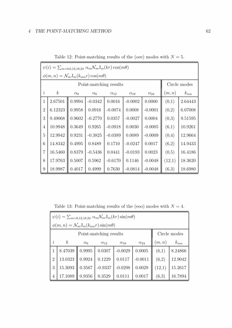
4 THE POINT-MATCHING METHOD 62
Table 12: Point-matching results of the (oee) modes with N = 5.
ψ(i) =∑m=0,6,12,18,24 αmNmJm(kr) cos(mθ)
φ(m,n) = NmJm(kmnr) cos(mθ)
Point-matching results Circle modes
i k α0 α6 α12 α18 α24 (m,n) kmn
1 2.67501 0.9994 -0.0342 0.0016 -0.0002 0.0000 (0,1) 2.64443
2 6.12323 0.9958 0.0916 -0.0074 0.0008 -0.0001 (0,2) 6.07008
3 9.49068 0.9602 -0.2770 0.0357 -0.0027 0.0004 (0,3) 9.51595
4 10.9948 0.3649 0.9265 -0.0918 0.0030 -0.0005 (6,1) 10.9261
5 12.9942 0.9231 -0.3825 -0.0389 0.0089 -0.0009 (0,4) 12.9664
6 14.8342 0.4995 0.8489 0.1710 -0.0247 0.0017 (6,2) 14.9433
7 16.5460 0.8379 -0.5436 0.0441 -0.0193 0.0023 (0,5) 16.4186
8 17.9763 0.5007 0.5962 -0.6170 0.1146 -0.0048 (12,1) 18.3620
9 18.9987 0.4017 0.4999 0.7630 -0.0814 -0.0048 (6,3) 18.6980
Table 13: Point-matching results of the (eoo) modes with N = 4.
ψ(i) =∑m=6,12,18,24 αmNmJm(kr) sin(mθ)
φ(m,n) = NmJm(kmnr) sin(mθ)
Point-matching results Circle modes
i k α6 α12 α18 α24 (m,n) kmn
1 8.47039 0.9995 0.0307 -0.0029 0.0005 (6,1) 8.24866
2 13.0323 0.9924 0.1229 0.0117 -0.0011 (6,2) 12.9042
3 15.3093 0.3567 -0.9337 -0.0298 0.0029 (12,1) 15.2617
4 17.1089 0.9356 0.3529 0.0111 0.0017 (6,3) 16.7894

4 THE POINT-MATCHING METHOD 63
Table 14: Point-matching results of the (ooe) modes with N = 5.
ψ(i) =∑m=3,9,15,21,27 αmNmJm(kr) sin(mθ)
φ(m,n) = NmJm(kmnr) sin(mθ)
Point-matching results Circle modes
i k α3 α9 α15 α21 α27 (m,n) kmn
1 6.90190 0.9975 -0.0705 0.0034 -0.0006 0.0001 (3,1) 7.01586
2 10.5062 0.9908 0.1342 -0.0160 0.0016 -0.0001 (3,2) 10.7336
3 13.7697 0.9082 -0.4215 0.0704 -0.0047 0.0006 (3,3) 14.3120
4 14.9895 0.4625 0.8811 -0.0988 0.0002 -0.0002 (9,1) 14.6849
5 17.2330 0.9058 -0.4163 -0.0774 0.0182 -0.0014 (3,4) 17.8399
6 19.0686 0.5391 0.8164 0.2045 -0.0319 0.0010 (9,2) 18.9591
been done by dividing the 30◦ triangle modes up according to the edge conditions and
ordering them according to the cutoff wave number. The circular modes Jm(kmnr) cos(mθ)
and Jm(kmnr) sin(mθ) have m diametrical nodes and n − 1 interior circular nodes. The
diametrical nodes (antinodes) translate directly into Dirichlet (Neumann) conditions along
edges B and C of the 30◦-60◦-90◦ triangle. However, the circular nodes do not have such a
simple interpretation. Although the triangular modes do not possess circular nodes, a loose
connection may be drawn if we compare the typical wavelengths (which depend upon the
eigenvalue) in the different shapes.
Second, inscribed and circumscribed circles provide, respectively, upper and lower bounds
of the hexagon eigenvalues ([4], for example). These bounds are certainly not very tight and
are not used in this project. A failing of this bounding method is that it is not a priori
evident which eigenvalue is bounded, since the mapping is not unique.
Finally, the comparison between the modes can provide great insight into devising accu-
rate methods of solution. The point-matching method provides an appropriate example.
How may the one-to-one correspondence be shown? And how may the uniqueness fail?
First, imagine that the boundary of each region is continuously deformed from the 30◦-60◦-90◦
triangle to the 30◦ circular sector. Each intermediate shape (with appropriate edge condi-

4 THE POINT-MATCHING METHOD 64
tions) supports an infinite set of modes which may be associated in a one-to-one manner
with the modes of each nearby, nearly identical shape. Thus, given a definite method of de-
formation, each mode may be unambiguously and continuously followed (i.e. mapped) from
beginning to end and the one-to-one correspondence is established. This also demonstrates
that there is no creation or ‘destruction’ of modes in the mapping process. To be unique, the
one-to-one correspondence must be independent of the method of deformation. Uniqueness
may be proved if it can be shown that there are never any degenerate modes anywhere in the
mapping process. For, if this is true, every mode may be ordered according to the eigenvalue
and this ordering remains intact and the mapping is unique. The negative of the converse
is also valid; namely, if there may ever be any degenerate modes, then the mapping is not
unique. This is because the mapping depends upon the linear combination of degenerate
modes. Consider, for example, a definite method of deformation which supports two inter-
mediately degenerate modes, ψ and φ. Working from this intermediate shape, mapping the
linear combination aψ + bφ back to the circular and triangular modes depends upon the
(arbitrary) values of a and b. In effect, the levels may either actually cross or simply come
together and touch without crossing.41 Thus, the mapping in this case is ambiguous.
It is easy to see that the mapping is not unique. This is especially true for the closed-form
triangle modes since they may support arbitrarily high degeneracies. However, for any set
of modes, by simply choosing an isosceles right triangle (with appropriate edge conditions)
as an intermediate shape, every eigenvalue (with only one exception) may be brought into
coincidence with another. Thus, the mapping cannot be unique. The only exception occurs
with the lowest (ooo) mode, since this mode may never be degenerate for any domain.
For several modes, it was numerically verified that if the boundary is minimally deformed
from the 30◦-60◦-90◦ triangle to the 30◦ sector, the ordering of the eigenvalues is maintained.
The minimal deformation – of the edge connecting edges B and C – was given by
x2 + εy2 = εR2 + (1− ε) · 3
4(140)
where ε varies continuously from zero (triangle, x =√
3/2) to unity (sector, x2 + y2 = R2).
The ‘radial’ edges B and C remained intact and the area of the intermediate regions did not
41A ‘crossing’ indicates that the ordering of the eigenvalues changes in the mapping process.

4 THE POINT-MATCHING METHOD 65
vary by more than a few percent.
The coefficients αm(ε) and the eigenparameter k(ε) can be considered functions of the
parameter ε. When ε = 0, the values of the αm(ε = 0) and k(ε = 0) correspond to those
of those of the 30◦-60◦-90◦ triangle mode. At the other extreme, when ε = 1, the values
correspond to those of the 30◦ sector mode. And, since the basis functions are eigenfunctions
of the sector, only one of the coefficients is non-zero. Specifically, for each mode,
αm(ε = 1) = ±δmm′ (141)
where m′ is the m-value of the circular sector eigenmode to which the triangle mode is
mapped. The sign is determined using the normalization of Eq. (135).
Fig. 9 plots the approximate cutoff wavenumber and the values of the leading coefficients
as the eighth and ninth (oee) modes are mapped from the triangle to the sector. Observe that,
for example, the ninth (oee) mode is mapped into the ninth circular mode (m,n) = (6, 3)
despite the fact that α212(0) ≈ 0.58 is significantly greater than the other dominant terms
with α26(0) ≈ 0.25 and α2
0(0) ≈ 0.16. This provides an example of the fact that the largest
Pm = α2m for a given triangle mode does not necessarily determine the m-value of the asso-
ciated circular mode. Note that the computations were performed with N = 5, equiangular
matching points; and only the first four coefficients are plotted, since the fifth coefficient (in
both cases) is always less than 0.01 in magnitude.
4.5 High-Order Point-Matching Results
High order computations were performed for the non-closed form modes using the point-
matching method. In addition to the properties mentioned in the previous sections, two
important discoveries were made. One was that very tight bounds to the eigenvalues may
be obtained. The other was that, above a given order, the coefficients of the Fourier-Bessel
series follow a simple rule.
First, observe that the numerical values of the parameters (and their accura- cies) depend
upon the distribution as well as the number of matching points. For each approximate
eigenfunction ψN , with N fixed, there exists an optimal distribution of matching points.
This distribution is such that the maximum value of |ψN | or |∂ψN/∂x| along edge A is a
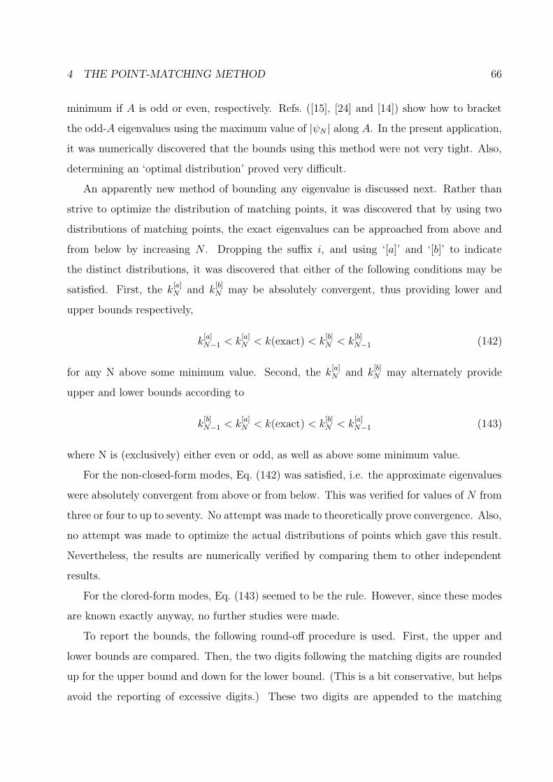
4 THE POINT-MATCHING METHOD 66
minimum if A is odd or even, respectively. Refs. ([15], [24] and [14]) show how to bracket
the odd-A eigenvalues using the maximum value of |ψN | along A. In the present application,
it was numerically discovered that the bounds using this method were not very tight. Also,
determining an ‘optimal distribution’ proved very difficult.
An apparently new method of bounding any eigenvalue is discussed next. Rather than
strive to optimize the distribution of matching points, it was discovered that by using two
distributions of matching points, the exact eigenvalues can be approached from above and
from below by increasing N . Dropping the suffix i, and using ‘[a]’ and ‘[b]’ to indicate
the distinct distributions, it was discovered that either of the following conditions may be
satisfied. First, the k[a]N and k
[b]N may be absolutely convergent, thus providing lower and
upper bounds respectively,
k[a]N−1 < k
[a]N < k(exact) < k
[b]N < k
[b]N−1 (142)
for any N above some minimum value. Second, the k[a]N and k
[b]N may alternately provide
upper and lower bounds according to
k[b]N−1 < k
[a]N < k(exact) < k
[b]N < k
[a]N−1 (143)
where N is (exclusively) either even or odd, as well as above some minimum value.
For the non-closed-form modes, Eq. (142) was satisfied, i.e. the approximate eigenvalues
were absolutely convergent from above or from below. This was verified for values of N from
three or four to up to seventy. No attempt was made to theoretically prove convergence. Also,
no attempt was made to optimize the actual distributions of points which gave this result.
Nevertheless, the results are numerically verified by comparing them to other independent
results.
For the clored-form modes, Eq. (143) seemed to be the rule. However, since these modes
are known exactly anyway, no further studies were made.
To report the bounds, the following round-off procedure is used. First, the upper and
lower bounds are compared. Then, the two digits following the matching digits are rounded
up for the upper bound and down for the lower bound. (This is a bit conservative, but helps
avoid the reporting of excessive digits.) These two digits are appended to the matching

4 THE POINT-MATCHING METHOD 67
Figure 9: Plots of the eighth and ninth (oee) eigenmodes as the cross section is deformedaccording to Eq. (140). The mapping is made as ε varies from zero (30◦-60◦-90◦ triangle) tounity (30◦ circular sector). Top: The eigenvalue mapping. Bottom: The coefficient mapping.
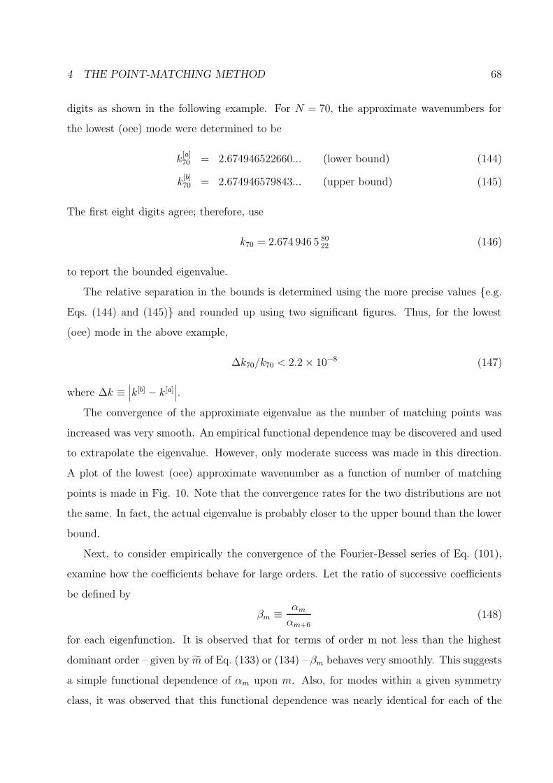
4 THE POINT-MATCHING METHOD 68
digits as shown in the following example. For N = 70, the approximate wavenumbers for
the lowest (oee) mode were determined to be
k[a]70 = 2.674946522660... (lower bound) (144)
k[b]70 = 2.674946579843... (upper bound) (145)
The first eight digits agree; therefore, use
k70 = 2.674 946 5 8022 (146)
to report the bounded eigenvalue.
The relative separation in the bounds is determined using the more precise values {e.g.
Eqs. (144) and (145)} and rounded up using two significant figures. Thus, for the lowest
(oee) mode in the above example,
∆k70/k70 < 2.2× 10⁻⁸ (147)
where ∆k ≡∣∣∣k[b] − k[a]
∣∣∣.
The convergence of the approximate eigenvalue as the number of matching points was
increased was very smooth. An empirical functional dependence may be discovered and used
to extrapolate the eigenvalue. However, only moderate success was made in this direction.
A plot of the lowest (oee) approximate wavenumber as a function of number of matching
points is made in Fig. 10. Note that the convergence rates for the two distributions are not
the same. In fact, the actual eigenvalue is probably closer to the upper bound than the lower
bound.
Next, to consider empirically the convergence of the Fourier-Bessel series of Eq. (101),
examine how the coefficients behave for large orders. Let the ratio of successive coefficients
be defined by
βm ≡αmαm+6
(148)
for each eigenfunction. It is observed that for terms of order m not less than the highest
dominant order – given by m of Eq. (133) or (134) – βm behaves very smoothly. This suggests
a simple functional dependence of αm upon m. Also, for modes within a given symmetry
class, it was observed that this functional dependence was nearly identical for each of the

4 THE POINT-MATCHING METHOD 69
Figure 10: Plot of the approximate wavenumber as a function of the number of matchingpoints for the lowest (oee) mode. This illustrates the convergence from above and frombelow using two different distributions of matching points. (Convergence for this mode wasactually verified up to N = 70.)

4 THE POINT-MATCHING METHOD 70
modes. The difference between the modes is of course indicated by different wavenumbers
and different leading order terms (i.e. the αm for m < m). Also, the larger the |βm| as m
increases, the more rapidly the series converges.
In Fig. 11, the ratio of coefficients βm is plotted for m-values from 6 to 394 for the
lowest (eoo) mode. This includes 49 terms. The number of matching points used in this
computation is N = 50. For simplicity, I use the notation mµ, where µ = 1, 2, · · · , N , in
which case, mµ = 6µ. Note that above µ = 40 (m = 240), the βm assume apparently
random values. This is probably a byproduct of the point-matching method, not numerical
‘round-off’.42 In fact, this random behavior of several of the highest order terms is present
in all computations, no matter what the value of N . More important is the behavior of the
first few terms (in this case, one) and the intermediate terms before the apparently erratic
behavior. Note that the values of βm for m > 6 are negative, indicating that the coefficients
alternate in sign. Also, with the normalization of Eq. (135), the value α6 ≈ 0.99954. Some
unsuccessful attempts were made to fit the smooth curve to elementary functions of m.43
The distributions of points which successfully bounded the eigenvalues are described
next. One set, which consistently gives lower bounds for each non-closed-form symmetry
class, were equally spaced points along edge A,
xµ =
√3
2and yµ =
1
2N
[µ− 1
2
](149)
for µ = 1, 2, · · · , N . These points exclude the end points and so may be used for each
symmetry class without modification. The other set of points, which consistently give com-
plementary upper bounds, are also equally spaced along edge A; however, they include the
end points of A only where appropriate,
xµ =
√3
2and yµ =
(µ−1)2(N−1)
for (*ee) modes
mu2N
for (*oe) modes
(µ−1)2N
for (*eo) modes
µ2(N−1)
for (*oo) modes
(150)
42The program MAPLE was used in the calculations. Setting the ‘Digits’ variable to increasingly larger
values from 20 up to 50 did not reduce the erratic behavior of the last few coefficients. Round-off error is
thus excluded.43For example, βm = A+B/m+ C/m2 + · · · did not work very well.

4 THE POINT-MATCHING METHOD 71
Figure 11: Plot of βm = αm/αm+1 for the lowest (eoo) mode using the approximation withN = 50. Fore convenience, on the abscissa, i = 1, 2, · · · , 49 is used where mi = 6i. Note thatthis mode has k ≈ 8.46825 and α6 ≈ 0.99954. Also, β6 ≈ 32.9871 and β12 ≈ −11.0693 areoff the vertical scale.
for µ = 1, 2, · · · , N . The excluded end points are locations where the edge conditions axe
satisfied trivially. (If they are included, the determinant ∆(k, {η}) vanishes identically.)
Note that the points of each distribution (149) and (150) are interleaved.
Although no mathematical proof is available, a heuristic argument is offered which ex-
plains why these distributions may give upper and lower bounds. The explanation is based
on the fact that increasing (decreasing) the area of the 30◦-60◦-90◦ decreases (increases) the
eigenvalue. Consider the slightly curved contour passing through the matching points where
the edge A conditions are enforced. Thus, if A is odd (or even), a node (or antinode) must
pass through the matching points and intersect with edges B and C. These ‘curved’ con-
tours, together with the radial edges, define two regions of slightly different shapes and sizes.
Although the eigenvalue depends upon the shape as well as the area, I conjecture that the
region with a slightly larger (smaller) area gives a slightly smaller (larger) eigenvalue. The
eigenfunctions appear to be most sensitive to the matching points near the intersections of
edges A and C. I also conjecture that the distribution given by Eq. (150) gives a contour
which bounds a slightly smaller region than that given by Eq. (149). Both regions approach
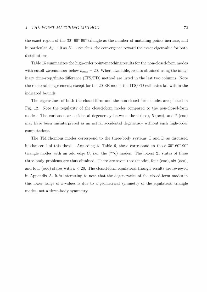
4 THE POINT-MATCHING METHOD 72
the exact region of the 30◦-60◦-90◦ triangle as the number of matching points increase, and
in particular, δy → 0 as N →∞; thus, the convergence toward the exact eigenvalue for both
distributions.
Table 15 summarizes the high-order point-matching results for the non-closed-form modes
with cutoff wavenumber below kmax = 20. Where available, results obtained using the imag-
inary time-step/finite-difference (ITS/FD) method are listed in the last two columns. Note
the remarkable agreement; except for the 20-EE mode, the ITS/FD estimates fall within the
indicated bounds.
The eigenvalues of both the closed-form and the non-closed-form modes are plotted in
Fig. 12. Note the regularity of the closed-form modes compared to the non-closed-form
modes. The curious near accidental degeneracy between the 4-(eeo), 5-(oee), and 2-(eoo)
may have been misinterpreted as an actual accidental degeneracy without such high-order
computations.
The TM rhombus modes correspond to the three-body systems C and D as discussed
in chapter I of this thesis. According to Table 6, these correspond to those 30◦-60◦-90◦
triangle modes with an odd edge C, i.e., the (**o) modes. The lowest 21 states of these
three-body problems are thus obtained. There are seven (eeo) modes, four (eoo), six (oeo),
and four (ooo) states with k < 20. The closed-form equilateral triangle results are reviewed
in Appendix A. It is interesting to note that the degeneracies of the closed-form modes in
this lower range of k-values is due to a geometrical symmetry of the equilateral triangle
modes, not a three-body symmetry.

4 THE POINT-MATCHING METHOD 73
Table 15: Summary of the bounded eigenvalues obtained using the point-matching method.Only the non-closed-form modes with k < 20 are given here. Where available, the lastcolumns list the mode and cutoff wavenumber (rounded to at least seven digits), obtainedwith the finite-difference method (Chapter II).
Point-matching Finite-difference
mode N kN ∆kN/kN mode k
1-(oee) 70 2.674 946 5 8022 2.2× 10⁻⁸ 1-EE 2.674 946 5
2-(oee) 20 6.123 0 2111 1.5× 10⁻⁶ 3-EE 6.123 018
3-(oee) 20 9.489 9288 3.4× 10⁻⁶ 6-EE 9.489 908
4-(oee) 20 10.993 9 8652 3.1× 10⁻⁶ 7-EE 10.993 98
5-(oee) 20 12.993 1206 3.4× 10⁻⁶ 10-EE 12.993 10
6-(oee) 20 14.831 5240 7.0× 10⁻⁶ 12-EE 14.831 48
7-(oee) 20 16.544 5548 3.4× 10⁻⁶ 15-EE 16.544 52
8-(oee) 20 17.970 3513 1.2× 10⁻⁵ 18-EE 17.970 28
9-(oee) 25 18.998 38 5901 2.6× 10⁻⁷ 20-EE 18.998 36
1-(eeo) 50 4.989 84 6859 1.5× 10⁻⁷
2-(eeo) 20 9.155 8 1201 1.2× 10⁻⁶
3-(eeo) 20 11.851 2210 1.1× 10⁻⁵
4-(eeo) 20 13.008 789 6250 8.9× 10⁻⁹
5-(eeo) 20 16.327 2616 5.4× 10⁻⁶
6-(eeo) 20 17.050 5646 5.2× 10⁻⁶
7-(eeo) 20 18.777 8855 1.8× 10⁻⁵
1-(ooe) 50 6.901 40 3523 1.7× 10⁻⁷ 2-EO 6.901 403
2-(ooe) 20 10.504 9 9753 4.1× 10⁻⁶ 5-EO 10.504 98
3-(ooe) 20 13.766 4331 8.2× 10⁻⁶ 9-EO 13.76639
4-(ooe) 20 14.989 1 5845 7.9× 10⁻⁷ 11-EO 14.989 15
5-(ooe) 20 17.227 7133 1.0× 10⁻⁵ 14-EO 17.227 65
6-(ooe) 20 19.065 4433 5.2× 10⁻⁵ 17-EO 19.065 39
1-(eoo) 50 8.468 24 7950 3.4× 10⁻⁷
2-(eoo) 20 13.029 6357 3.9× 10⁻⁶
3-(eoo) 20 15.298 9675 1.3× 10⁻⁵
4-(eoo) 20 17.108 6 1106 2.4× 10⁻⁷

4 THE POINT-MATCHING METHOD 74
Figure 12: The spectrum of the 30◦-60◦-90◦ trianglular region with the eight possible edgeconditions. The closed-form and non-closed-form modes are listed in the left and right halvesrespectivley. Note the regular behavior of the closed-form spectrum. The only degeneraciesoccur in the closed-form eigenvalues; however, note the near degeneracy of the 4-(eeo),5-(oee), and 2-(eoo) modes.
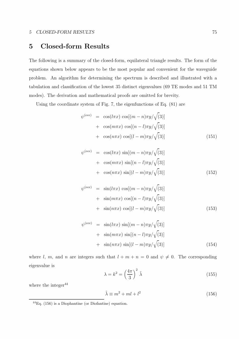
5 CLOSED-FORM RESULTS 75
5 Closed-form Results
The following is a summary of the closed-form, equilateral triangle results. The form of the
equations shown below appears to be the most popular and convenient for the waveguide
problem. An algorithm for determining the spectrum is described and illustrated with a
tabulation and classification of the lowest 35 distinct eigenvalues (69 TE modes and 51 TM
modes). The derivation and mathematical proofs are omitted for brevity.
Using the coordinate system of Fig. 7, the eigenfunctions of Eq. (81) are
ψ(eee) = cos(lπx) cos[(m− n)πy/√
(3)]
+ cos(mπx) cos[(n− l)πy/√
(3)]
+ cos(nπx) cos[(l −m)πy/√
(3)] (151)
ψ(eee) = cos(lπx) sin[(m− n)πy/√
(3)]
+ cos(mπx) sin[(n− l)πy/√
(3)]
+ cos(nπx) sin[(l −m)πy/√
(3)] (152)
ψ(eee) = sin(lπx) cos[(m− n)πy/√
(3)]
+ sin(mπx) cos[(n− l)πy/√
(3)]
+ sin(nπx) cos[(l −m)πy/√
(3)] (153)
ψ(eee) = sin(lπx) sin[(m− n)πy/√
(3)]
+ sin(mπx) sin[(n− l)πy/√
(3)]
+ sin(nπx) sin[(l −m)πy/√
(3)] (154)
where l, m, and n are integers such that l + m + n = 0 and ψ 6= 0. The corresponding
eigenvalue is
λ = k2 =(
4π
3
)2
λ (155)
where the integer44
λ ≡ m2 +ml + l2 (156)
44Eq. (156) is a Diophantine (or Diofantine) equation.
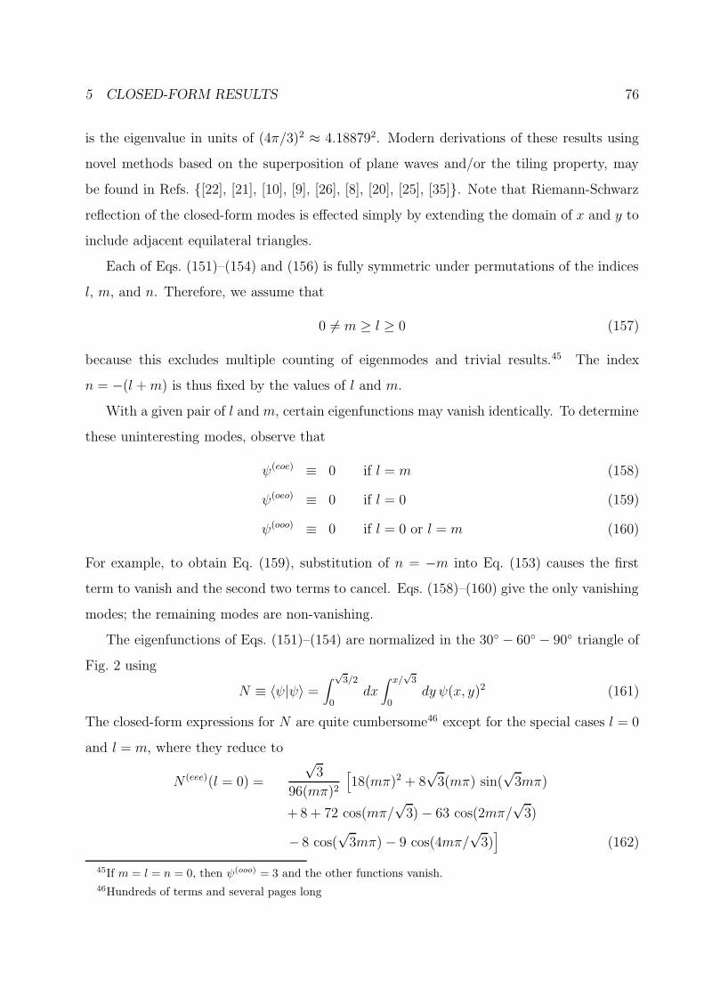
5 CLOSED-FORM RESULTS 76
is the eigenvalue in units of (4π/3)2 ≈ 4.188792. Modern derivations of these results using
novel methods based on the superposition of plane waves and/or the tiling property, may
be found in Refs. {[22], [21], [10], [9], [26], [8], [20], [25], [35]}. Note that Riemann-Schwarz
reflection of the closed-form modes is effected simply by extending the domain of x and y to
include adjacent equilateral triangles.
Each of Eqs. (151)–(154) and (156) is fully symmetric under permutations of the indices
l, m, and n. Therefore, we assume that
0 6= m ≥ l ≥ 0 (157)
because this excludes multiple counting of eigenmodes and trivial results.45 The index
n = −(l +m) is thus fixed by the values of l and m.
With a given pair of l and m, certain eigenfunctions may vanish identically. To determine
these uninteresting modes, observe that
ψ(eoe) ≡ 0 if l = m (158)
ψ(oeo) ≡ 0 if l = 0 (159)
ψ(ooo) ≡ 0 if l = 0 or l = m (160)
For example, to obtain Eq. (159), substitution of n = −m into Eq. (153) causes the first
term to vanish and the second two terms to cancel. Eqs. (158)–(160) give the only vanishing
modes; the remaining modes are non-vanishing.
The eigenfunctions of Eqs. (151)–(154) are normalized in the 30◦ − 60◦ − 90◦ triangle of
Fig. 2 using
N ≡ 〈ψ|ψ〉 =∫ √3/2
0dx∫ x/
√3
0dy ψ(x, y)2 (161)
The closed-form expressions for N are quite cumbersome46 except for the special cases l = 0
and l = m, where they reduce to
N (eee)(l = 0) =
√3
96(mπ)2
[18(mπ)2 + 8
√3(mπ) sin(
√3mπ)
+ 8 + 72 cos(mπ/√
3)− 63 cos(2mπ/√
3)
− 8 cos(√
3mπ)− 9 cos(4mπ/√
3)]
(162)
45If m = l = n = 0, then ψ(ooo) = 3 and the other functions vanish.46Hundreds of terms and several pages long

5 CLOSED-FORM RESULTS 77
N (eoe)(l = 0) =
√3
96(mπ)2
[18(mπ)2 + 8
√3(mπ) sin(
√3mπ)
+ 8− 72 cos(mπ/√
3) + 63 cos(2mπ/√
3)
− 8 cos(√
3mπ) + 9 cos(4mπ/√
3)]
(163)
N (eee)(l = m) =
√3
96(mπ)2
[18(mπ)2 + 2
√3(mπ)
{sin(2
√3mπ)
+ 4 sin(√
3mπ)}
+ 9− 9 cos(2√
3mπ)]
(164)
N (oeo)(l = m) =
√3
96(mπ)2
[18(mπ)2 − 2
√3(mπ)
{sin(2
√3mπ)
+ 4 sin(√
3mπ)}− 9 + 16 cos(
√3mπ)
− 7 cos(2√
3mπ)]
(165)
The asymptotic value of Eqs. (162)–(163) is N = 3√
3/16 +O(1/m). If m > l > 0, then the
asymptotic value is N = 3√
3/32 +O(1/m) +O(1/l). For small values of m, the values of
N do not vary by much more than ten percent of these asymptotic values. These results do
not appear in the published literature.
There are two types of accidental degeneracy. The first type occurs if the Diophantine
problem, namely Eq. (156) subject to Eq. (157), admits multiple solutions. The second type
occurs if two or more distinct modes with the same l and m do not belong to the mixed
representation of S3. To determine the exact nature of the spectrum and the classification
of the closed-form modes, we need some results from elementary number theory.
Every integer λ of the form m2 +ml + l2 has the unique Gaussian factorization
λ =
[3α ·
r∏
i=1
pγii
]· 2β0 ·
k∏
j=1
qβjj
2
(166)
where the p and q are rational primes congruent to respectively 1 and 5, modulo 6.47 (The
converse is true, any number given by Eq. (166) is an eigenvalue λ of the form m2 +ml + l2.)
The lowest values of these primes are
p = 7, 13, 19, 31, 37, 43, 61, ... (167)
q = 5, 11, 17, 23, 29, 41, 47, ... (168)
47In other words, p and q are primes of the form p = 6µ+ 1 and q = 6µ− 1 where µ = 1, 2, 3, ....

5 CLOSED-FORM RESULTS 78
Table 16: The accidental degeneracy of an eigenvalue within each symmetry class.
α γ g(eee) g(eoe) g(oeo) g(ooo)
even even (g + 2)/4 (g + 2)/4 (g − 2)/4 (g − 2)/4
odd even (g + 2)/4 (g − 2)/4 (g + 2)/4 (g − 2)/4
odd g/4 g/4 g/4 g/4
The exponents α (of 3) and the r non-zero γ ≡ {γi|i = 1, 2, 3, ..., r} (of the pi) play an
essential role in this formalism. We use the notation that if all of the γi are even, then γ
is said to be ’even’; while if some or all of the γi are odd, then γ is said to be ’odd’. To
illustrate, if α and γ are both even, then λ is the square of an integer.
A number-theoretic result using integer-domain ring theory is that the total number of
distinct TE and TM modes belonging to a given eigenvalue λ is
g = 2r∏
i=1
[γi + 1] (169)
Furthermore, the number of distinct solutions of the Diophantine problem, Eqs. (156) and
(157), is (g + 2)/4 is γ is even and g/4 if γ is odd. Table 16 lists the accidental degeneracy
of an eigenvalue within each symmetry class. Discussion and proof of these results may be
found in Refs. {[6], [31], [26]}.Multiple solutions of the Diophantine problem yield linearly independent solutions within
each symmetry class; however, degenerate eigenfunctions are not necessarily orthogonal.48
The Gram-Schmidt orthogonalization procedure {[22], for example} may be used to obtain
orthogonal functions.
The equilateral triangle eigenvalue problem is invariant under the geometrical point
group S3, i.e., the symmetry group of degree three [20]. Thus it is helpful to further classify
the closed-form modes according to the irreducible representations of S3 – namely, the one-
dimensional symmetric S, the one-dimensional antisymmetric A, and the two-dimensional
mixed M representations. According to S3 invariance, the only geometrical degeneracy
48The TE (TM) modes within separate symmetry classes are orthogonal by construction.

5 CLOSED-FORM RESULTS 79
occurs in the pairs of mixed modes; any other degeneracy is accidental.
The symmetric and antisymmetric eigenfunctions have respectively even and odd lines
connecting each of the three vertices to the center of the opposite edge of the equilateral
triangle. A judicious linear combination of the degenerate mixed modes is made such that
each pair is split into separate symmetry classes [25]. Specifically, these mixed modes,Meand
Mo, have exactly one even and one odd line, respectively, connecting a vertex to the center
of the opposite edge.
If α > 0 for a given eigenvalue, then the modes belong to either the symmetric or
antisymmetric representations. But, if α = 0, then the modes come in pairs of mixed modes.
The classification scheme is summarized in Table 17. The only geometrical degeneracy due
to S3 invariance occurs with pairs of either TE (Me-TE and Mo-TE) or TM (Me-TM and
Mo-TM) modes. Every other degeneracy is accidental, including multiple sets of mixed
modes.
The reason why modes with α = 0 belong to the M representation, while those with
α > 0 belong to either the Aor Srepresentations, is related to a reflect-and-shrink property.
Indeed, any closed form 30◦ − 60◦ − 90◦ triangle mode ψ with eigenvalue λ may be reflected
three times to form another larger 30◦ − 60◦ − 90◦ triangle mode. If this is reduced to the
size of the original triangle (using (x, y)→ (x/3, y/3)), we obtain an Aor Smode ψ ′ with
eigenvalue 3λ. Every Sand Amode may be obtained this way.
The edge conditions of ψ determine the S3 symmetry and boundary conditions of ψ′.
Thus, if the edge conditions of ψ are (eee), (eoe), (oeo), or (ooo), then, the edge conditions
of ψ′ are (eee)=S-TE, (oeo)=S-TM, (eoe)=A-TE, or (ooo)=A-TM, respectively. If α = 0,
then this mode cannot be obtained using the reflect-and-shrink property of a lower mode
and must consequently be an Mmode, since it is neither and Snor an Amode. Because not
all inverses exist, the reflect-and-shrink operations do not form a group.
Tabulation of the eigenmodes is obtained using the following procedure: First, select
a number λmax > λ and fill in the triangular array as shown in Fig. 13 keeping in mind
Eq. (157). In this example, λmax = 100. Note that λ = 49 and 91 appear twice.
Second, arrange the possible l, m, and λ as shown in the first three columns of Table 18.
In the first column, prime factor each λ according to Eq. 166.

5 CLOSED-FORM RESULTS 80
Table 17: Classification of the closed-form modes according to S3 based on the value of α.
eee eoe oeo ooo
α = 0 Me-TE Mo-TE Me-TM Mo-TM
α > 0 S-TE A-TE S-TM A-TM
9 81 91
8 64 73 84 97
7 49 57 67 79 93
6 36 43 52 63 76 91
5 25 31 39 49 61 75
4 16 21 28 37 48 –
3 9 13 19 27 – –
2 4 7 12 – – –
1 1 3 – – – –
m/l 0 1 2 3 4 5
Figure 13: Tabulation of the possible λ < 100.

5 CLOSED-FORM RESULTS 81
Third, for each pair l and m, determine the modes of Eqs. (151)–(154) which vanish
identically by applying the rules of Eqs. (158)–(160). Mark a ’–’ in columns 4-6 of Table 18
for each vanishing mode.
Finally, classify each non-vanishing mode according to S3, using the value of α and
Table 17. From Table 18, we observe that there are five possibilities for a given pair of l and
m. They are illustrated with (l, m) = (0, 1), (1, 1), (1, 2), (0, 3), and (1, 4).
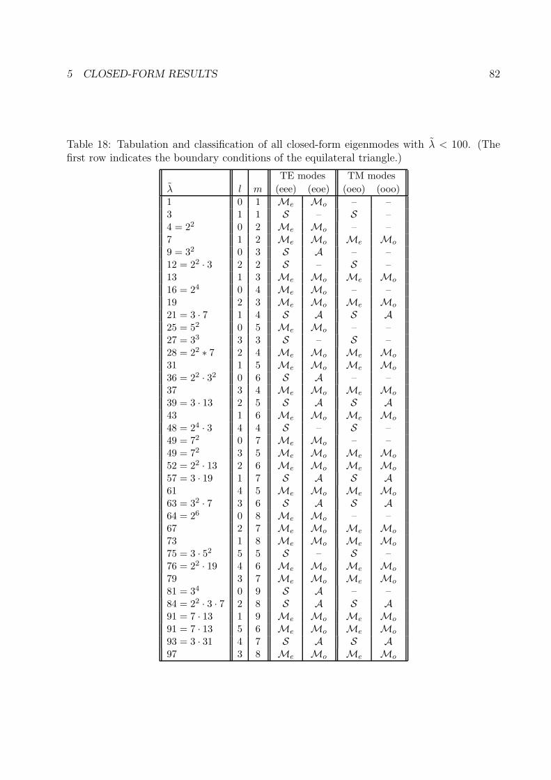
5 CLOSED-FORM RESULTS 82
Table 18: Tabulation and classification of all closed-form eigenmodes with λ < 100. (Thefirst row indicates the boundary conditions of the equilateral triangle.)
TE modes TM modes
λ l m (eee) (eoe) (oeo) (ooo)
1 0 1 Me Mo – –3 1 1 S – S –4 = 22 0 2 Me Mo – –7 1 2 Me Mo Me Mo
9 = 32 0 3 S A – –12 = 22 · 3 2 2 S – S –13 1 3 Me Mo Me Mo
16 = 24 0 4 Me Mo – –19 2 3 Me Mo Me Mo
21 = 3 · 7 1 4 S A S A25 = 52 0 5 Me Mo – –27 = 33 3 3 S – S –28 = 22 ∗ 7 2 4 Me Mo Me Mo
31 1 5 Me Mo Me Mo
36 = 22 · 32 0 6 S A – –37 3 4 Me Mo Me Mo
39 = 3 · 13 2 5 S A S A43 1 6 Me Mo Me Mo
48 = 24 · 3 4 4 S – S –49 = 72 0 7 Me Mo – –49 = 72 3 5 Me Mo Me Mo
52 = 22 · 13 2 6 Me Mo Me Mo
57 = 3 · 19 1 7 S A S A61 4 5 Me Mo Me Mo
63 = 32 · 7 3 6 S A S A64 = 26 0 8 Me Mo – –67 2 7 Me Mo Me Mo
73 1 8 Me Mo Me Mo
75 = 3 · 52 5 5 S – S –76 = 22 · 19 4 6 Me Mo Me Mo
79 3 7 Me Mo Me Mo
81 = 34 0 9 S A – –84 = 22 · 3 · 7 2 8 S A S A91 = 7 · 13 1 9 Me Mo Me Mo
91 = 7 · 13 5 6 Me Mo Me Mo
93 = 3 · 31 4 7 S A S A97 3 8 Me Mo Me Mo

REFERENCES 83
References
[1] M. Abromowitz and (editors) I. Stegun. Handbook of Mathematical Functions With
Formulas, Graphs, and Mathematical Tables. Dover, NY, 1972.
[2] R. H. T. Bates. The point-matching method for interior and exterior two-dimensional
boundary value problems. IEEE Trans. Microwave Theory and Tech., MTT-15:185–187,
1967.
[3] R. H. T. Bates. The theory of the point-matching method for perfectly conducting
waveguides and transmission lines. IEEE Trans. Microwave Theory and Tech., 6:294–
301, 1969.
[4] L. Bauer and E. L. Reiss. Cutoff wavenumbers and modes of hexagonal waveguides.
SIAM J. Appl. Math., 35:508–514, 1978.
[5] P. Berard. Analyse mathematique. – spectres et groups cristallographiques. C. R. Acad.
Sc. Paris, 288:1059–1060, 1979.
[6] E. D. Bolker. Elementary Number Theory. Benjamin, NY, 1970. Page 121.
[7] H. D. Conway. The bending, buckling, and flexural vibrations of simply supported
polygonal plates by point matching. Trans. ASME J. Appl. Mech., 83E:288–291, 1961.
[8] H. R. Krishnamurthy H. S. Mani and H. C. Verma. Exact solutions of the schrodinger
equation for a particle in a tetrahedral box. J. Phys. A: Math. Gen., 9:2131–2137, 1982.
[9] R. N. Hill. An exactly solvable one dimensional three-body problem with hard cores.
J. Math. Phys., 21:1083–1085, 1980.
[10] R. N. Hill. Systematic improvement of hall-post-stenschke lower bounds to eigenvalues
in the few-body problem. J. Math. Phys., 21:1070–1082, 1980.
[11] J. D. Jackson. Classical Electromagnetics, 2nd edition. John Wiley & Sons, 1962. See
chapter 8 for a discussion of the waveguide problem. This popular text does not mention
the equilateral triangle solutions.
REFERENCES 84
[12] Kosloff and Tal-ezer. A direct relaxation method for calculating eigenfunctions and
eigenvalues of the schrodinger equation on a grid. Chem. Phys. Let., 127:163–230, 1986.
[13] J. R. Kuttler and V. G. Sigilito. Eigenvalues of the laplacian in two dimensions. SIAM
Rev., 26:163–193, 1984.
[14] J. R. Kuttler and V. G. Sigillito. Bounding eigenvalues of elliptic operators. SIAM J.
Math. Anal., 9:768–773, 1978.
[15] P. Henrici L. Fox and C. Moler. Approximations and bounds for eigenvalues of elliptical
operators. SIAM J. Numer. Anal., 4:89–102, 1967.
[16] G. Lame. Lecons sur la theorie mathematique de l’elasticite des corps solides. Bachelier,
Paris, 1852.
[17] T. Larsen. On the relation between modes in rectangular, elliptical, and parabolic
waveguides and a mode-classifying system. IEEE Trans. Microwave Theory and Tech.,
MTT-20:379–384, 1972.
[18] P. A. Laura. Applications of the point-matching method in waveguide problems. IEEE
Trans. Microwave Theory and Tech., MTT-14:251, 1966.
[19] W-K. Li. Degeneracy in the particle-in-a-square problem. Am. J. Phys., 50:666, 1982.
[20] W-K. Li and S. M. Blinder. Solution of the schrodinger equation for a particle in an
equilateral triangle. J. Math. Phys., 26:2784–2786, 1985.
[21] Weigan Lin. Microwave Theory and Techniques. Science Press, Beijing, 1979. (In
Chinese).
[22] J. Mathews and R. L. Walker. Mathematical Methods for Physicists. Benjamin, NY,
1970.
[23] E. Merzbacher. Quantum Mechanics, second edition. John Wiley & Sons, NY, 1970.
[24] C. B. Moler and L. E. Payne. Bounds for eigenvalues and eigenvectors of symmetric
operators. IAM J. Numer. Anal., 5:64–71, 1968.

REFERENCES 85
[25] P. L. Overfelt and D. J. White. Te and tm modes of some triangular cross-section
waveguides using superposition of plane waves. IEEE Trans. Microwave Theory and
Tech., MTT-34:161–167, 1986.
[26] M. A. Pinsky. The eigenvalues of an equilateral triangle. SIAM J. Math. Anal., 11:819–
827, 1980.
[27] F. Pockels. Uber die partielle Differentialgleichung ∇2u+ k2u = 0 und deren Auftreten
in die mathematischen Physik. Teubner, Leipzig, 1891. (In German).
[28] F. Reif. Fundamentals of Statistical and Thermal Physics. McGraw-Hill, NY, 1965.
[29] S. A. Schelkunoff. Electromagnetic Waves. Van Nostrand Company, 1943. See reference
[25] for some noteworthy corrections.
[30] L. I. Schiff. Quantum Mechanics, third edition. McGraw-Hill, NY, 1968.
[31] G. B. Shaw. Degeneracy in the particle-in-a-box problem. J. Phys. A, 7:1537–1546,
1974.
[32] J. T. Stadter. Bounds to eigenvalues of rhombical membranes. J. SIAM Appl. Math.,
14:324–341, 1966.
[33] N. N. Lebedev (translated and edited by R. Silverman). Special Functions and Their
Applications. Dover, NY, 1972.
[34] J. W. Turner. On the quantum particle in a polyhedral box. J. Phys. A: Math. Gen.,
17:2791–2797, 1984.
[35] M. Pauri V. Amar and A. Scoitti. Schrodinger equation for convex plane polygons:
A tiling method for the derivation of eigenvalues and eigenfunctions. J. Math. Phys.,
32:2442–2449, 1991.
[36] G. N. Watson. A Treatise on the Theory of Bessel Functions, second edition. Cambridge
University Press, London, 1962.
REFERENCES 86
[37] R. F. Millar (with reply by R. H. T. Bates). On the legitamacy of an assumption
underlying the point-matching method. IEEE Trans. Microwave Theory and Tech.,
MTT-18:325–327, 1970.
[38] H. Y. Yee and N. F. Audeh. Uniform waveguides with arbitrary cross-section considered
by the point-matching method. IEEE Trans. Microwave Theory and Tech., MTT-
13:847–851, 1965.
[39] J. Zhang and J. Fu. Comments on ‘te and tm modes of some triangular cross-section
waveguides using supperposition of plane waves’. IEEE Trans. Microwave Theory and
Tech., 39:612–613, 1991.
![Unique continuation for the Helmholtz equation using a ... · Unique continuation for the Helmholtz equation using ... I Laplace equation [Burman’14] ... Unique continuation for](https://static.documents.pub/doc/80x56/5ae0fc9a7f8b9a595d8b4a83/unique-continuation-for-the-helmholtz-equation-using-a-continuation-for-the.jpg)


![Green’s Functionof3-D Helmholtz Equation for … · arXiv:math/0408186v1 [math.AP] 13 Aug 2004 Green’s Functionof3-D Helmholtz Equation for Turbulent Medium: Application toOptics](https://static.documents.pub/doc/80x56/5b85b6787f8b9af12d8b5a65/greens-functionof3-d-helmholtz-equation-for-arxivmath0408186v1-mathap.jpg)


