Spatiotemporal Analysis of Drought Variability over...

Pakistan Journal of Meteorology Vol. 13, Issue 25: Jul, 2016

51

Spatiotemporal Analysis of Drought Variability over Pakistan by Standardized Precipitation Index (SPI)

Haroon, M. A.1, Z. Jiahua2

Abstract

This study examined the spatial and temporal variability of drought occurrences over Pakistan

during 1960-2013.For this purpose, standardized precipitation index on 3 monthly time scale (SPI3)

was calculated form the observed precipitation data. The prevai ling wetness and dryness conditions

on provincial scale were identified by respective SPI3 time series. The spatio -temporal variability

of SPI3 values over the entire country was analyzed by principal component analysis (PCA).We

choose first three dominant modes those explain 45.8 % variability in the data. The first dominant

spatial pattern (EOF1) scores are positively correlated with the regions getting higher precipitation

amount in Pakistan. The second dominant pattern represented by component EOF2 divi des the

whole country into northern and southern regions. The distribution of third spatial pattern (EOF3)

divides the whole country into north, south and central parts. All the PCA time series did not display

any significant linear trend but however there are some cyclic patterns present in the data as

revealed by spectral analysis. There is a major cycle of 10.7 years in the occurrence of drought

intensive period possibly related to solar cycle of 11 years in sunspot activity in which a weak

sunspot activity leads to a strong rainfall variability. The second dominant cycle of 6.1 years is

present in SPI3 time series that could be explained with the help of El Nino southern oscillation

whose periodicity lies in the range of 3-6 years. Another cycle of 2.7 years in rainfall variability

could be explained with the help of Quasi-biennial oscillation (QBO) that is a cyclic phenomenon

of reversal of winds between easterlies to westerlies over the equatorial stratosphere. These

highlighted spatio-temporal patterns of drought incidences and their periodic behavior would help

policy makers to implement well-coordinated water resources planning and drought preparedness

strategies over the country to mitigate its possible adverse impacts.

Key Words: Pakistan; Drought; Standardized Precipitation Index; Principal component analysis; Spectral analysis.

Introduction

Drought is a natural climatic phenomenon that may occur worldwide but its adverse impacts vary from region to region (Wilhite 1997). The natural imbalance between demand and supply of water in an ecosystem due to persistent below normal precipitation results into dry conditions in the region. The situation become worsens if these conditions persist for several years. Thus, it is very important to assess and monitor the drought conditions in a particular region on continuous basis so that the adverse impacts could be prevented. There are many studies in the literature about drought and the scientists proposed many indices to quantify drought occurrences (Gibbs & Maher, 1967; Palmer, 1965, 1968; Shafer & Dezman, 1982).

The standardized precipitation index (SPI) proposed by McKee et al. (1993) is one of the indeces that is most widely used in drought studies. The main reasons behind its wide acceptance include: it is very easy to calculate based only on precipitation data, the comparison could be made among different regions since it is a standardized index and it could deal with different drought types on the basis of different SPI time scales. In the past, many studies in different regions of the world investigated the spatial and temporal variability of drought phenomenon. The studies like (Lloyd-Hughes and Saunders 2002; Bonaccorso et al. 2003; Piccarreta et al. 2004; Bordi et al. 2006; Vicente-Serrano and Cuadrat-Prats 2007; Vergni and Todisco 2011) presented an overall decreasing linear trend in drier conditions over Europe as observed in SPI time

1 [email protected], Pakistan Meteorological Department, Pitras Bukhari Road, Sector H-8/2, Islamabad, Pakistan. 2 Institute of Remote Sensing and Digital Earth, CAS, Beijing, China.

Spatiotemporal Analysis of Drought Variability over Pakistan by Standardized Precipitation Index (SPI) Vol. 13

52

series. But despite the similar observed trend, spatial variability of drought events vary from region to region that must be evaluated for effective planning and mitigation purposes.

The principal component analysis (PCA) is a multivariate technique often used in atmospheric and meteorological science to identify spatio-temporal patterns in the data. The purpose of PCA is to reduce the original variable into smaller number of uncorrelated components in terms of keeping maximum variability into account. PCA technique project the data into a new space called principal component space. The Eigen vectors calculated from the covariance matrix of the data form the basis of the new space. The first principal component accounts for the maximum possible variance in the data. An inspection of the first several principal components that account for the majority of the variance of the transformed variances enables identification of the major spatial pattern and temporal modes in a high-dimensional data-set. The application of PCA could be found in literature as Bonaccorso et al. (2003), Vicente-Serrano. (2006), and Santos et al. (2010).Also the presence of dry and wet cycles in PCA temporal modes could be highlighted by applying spectral analysis (Fleming et al.,2002).

In this paper, SPI time series at different time scales (3, 6, 12 months) are evaluated and analyzed to identify spatiotemporal variability of droughts in Pakistan. The analyses were based on the precipitation data collected from Pakistan Meteorological Department (PMD) for the period 1961 to 2013 at 51 climatic stations uniformly distributed over the entire country. PCA analysis was performed over SPI time series that was calculated over the entire country in order to find dominant spatial and temporal patterns in the data and spectral analysis revealed the presence of major cycles present in the data.

Materials and Methods

Study Area and Data

Pakistan is located in South Asia and stretches between (23o - 38o) North latitude and (61o - 78o) East longitude and covers an area of (796096) square kilometer. In the south, it borders with Arabian Sea having (650) miles coast line and in the north it stretches to Hindukush-Karakorum-Himalaya (H.K.H) region. It shares the border in the East with India, in the west with Afghanistan and Iran and in north with China.

Climate of Pakistan

The climate of Pakistan has great regional variations as shown in Figure 1.The climate is divided into four seasons, the hot dry spring (MAM), summer season (JJA) that receive monsoon precipitation,

Figure 1: Pakistan Map of Köppen - Geiger climate classification (K.P.K: Khyber Pakhtunkhwa, AJ&K:

Azad Jammu & Kashmir, G.B: Gilgit Baltistan (Peel et al., 2007).

Issue 25 Haroon, M. A., Z. Jiahua

53

autumn season (SON) and winter season (DJF). The climate in Pakistan is characterized by hot summers and cold winters. The extreme northern part of Pakistan is generally cold due to the presence of snowcapped mountains and wet while the southern part is hot and dry.

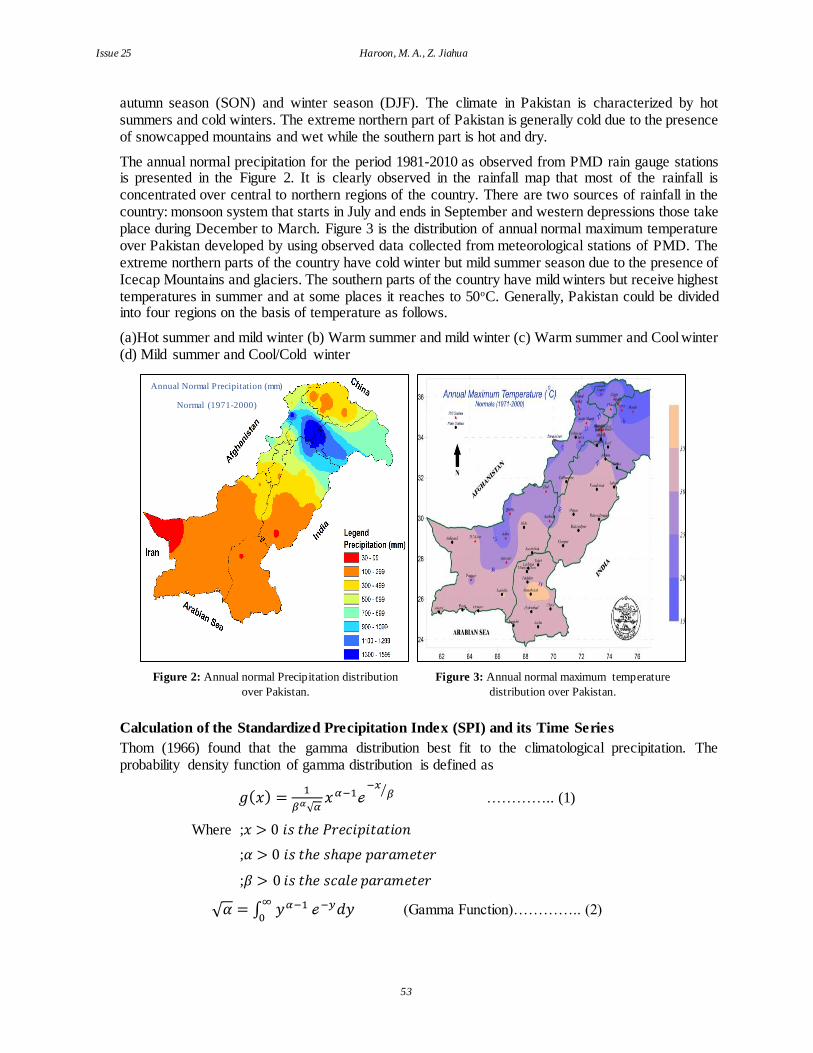
The annual normal precipitation for the period 1981-2010 as observed from PMD rain gauge stations is presented in the Figure 2. It is clearly observed in the rainfall map that most of the rainfall is concentrated over central to northern regions of the country. There are two sources of rainfall in the country: monsoon system that starts in July and ends in September and western depressions those take place during December to March. Figure 3 is the distribution of annual normal maximum temperature over Pakistan developed by using observed data collected from meteorological stations of PMD. The extreme northern parts of the country have cold winter but mild summer season due to the presence of Icecap Mountains and glaciers. The southern parts of the country have mild winters but receive highest temperatures in summer and at some places it reaches to 50oC. Generally, Pakistan could be divided into four regions on the basis of temperature as follows.

(a)Hot summer and mild winter (b) Warm summer and mild winter (c) Warm summer and Cool winter (d) Mild summer and Cool/Cold winter

Calculation of the Standardized Precipitation Index (SPI) and its Time Series

Thom (1966) found that the gamma distribution best fit to the climatological precipitation. The probability density function of gamma distribution is defined as

𝑔(𝑥) =1

𝛽𝛼√𝛼𝑥 𝛼−1ℯ

−𝑥𝛽⁄

………….. (1)

Where ;𝑥 > 0 𝑖𝑠 𝑡ℎ𝑒 𝑃𝑟𝑒𝑐𝑖𝑝𝑖𝑡𝑎𝑡𝑖𝑜𝑛

;𝛼 > 0 𝑖𝑠 𝑡ℎ𝑒 𝑠ℎ𝑎𝑝𝑒 𝑝𝑎𝑟𝑎𝑚𝑒𝑡𝑒𝑟

;𝛽 > 0 𝑖𝑠 𝑡ℎ𝑒 𝑠𝑐𝑎𝑙𝑒 𝑝𝑎𝑟𝑎𝑚𝑒𝑡𝑒𝑟

√𝛼 = ∫ 𝑦𝛼−1∞

0ℯ−𝑦𝑑𝑦 (Gamma Function)………….. (2)

Figure 2: Annual normal Precipitation distribution

over Pakistan.

Figure 3: Annual normal maximum temperature

distribution over Pakistan.

Annual Normal Precipitation (mm)

Normal (1971-2000)


54

The shape and scale parameters of the gamma distribution function can be estimated for each station and time under consideration by using the formulae

𝛼 =1

4𝐴[1 + √1 +

4𝐴

3] ………….. (3)

𝛽 =𝑋

𝑎 …..………. (4)

𝐴 = ln(𝑋) −∑ ln(𝑥)

𝑛 …………. (5)

n=Number of Precipitation observation

The values of these parameters are then used to find resultant commutative probability distribution function G(x) of the incomplete gamma function as

𝐺(𝑥) = ∫ 𝑔(𝑥)𝑥

0 𝑑𝑥 =1

𝛽𝛼√𝛼∫ 𝑥𝛼−1ℯ

−𝑥𝛽⁄𝑥

0 𝑑𝑥 ……. (6)

Since gamma function is undefined at x=0, but the precipitation distribution may contain zero, therefore commutative probability distribution function for precipitation is defined as

𝐻(𝑥) = 𝑞 + (1 − 𝑞)𝐺(𝑥) ………. (7)

The probability of a zero in H(x) is included by the factor (q). This probability is then transformed to Z value having zero mean and variance of one and is defined as Standardized Precipitation Index (SPI). More details about mathematical formulation could be found in Edwards and McKee (1997) or Lloyd-Hughes and Saunders (2002).It was firstly calculated by McKee et al. (1993) for 3, 6, 12, 24, and 48 months timescales to address the different impacts, but the index can be calculated for any weekly or monthly timescale. Since SPI values are standardized and are achieved by applying probability distribution function on historical data of precipitation at any location, therefore it is equally suited for comparison of any climatic conditions may they be wet or dry. The positive SPI values are related to greater than median precipitation and negative values are related to less than median precipitation (Bordi & Sutera, 2001). The magnitude of SPI value can also be linked to the severity of a current event since the frequency of occurrence of each event is known in a historical perspective. This is one of the features that distinguishes SPI from the other indices. The SPI is now the accepted standard worldwide and is recommended by World Meteorological Organization (WMO, 2009) as the primary meteorological drought index to be used by national meteorological and hydrological agencies to monitor drought.

Table 1: Drought classification according to SPI

SPI Index Value Class

Non Drought

SPI >= 2.0 Extremely Wet

1.5 =< SPI <= 1.99 Severely Wet

1.0 =< SPI <= 1.49 Moderately Wet

0.5 =< SPI <= 0.99 Slightly Wet

-0.49 =< SPI <= 0.49 Normal

Drought

-0.5 =< SPI <= -0.99 Mild Drought

-1.0 =< SPI <= -1.49 Moderate Drought

-1.5 =< SPI <= -1.99 severe Drought

SPI <= -2.00 Extreme Drought

McKee et al (1993) used the classification system shown in the Table 1 that defines multiple categories of drought in terms of SPI values. They also defined the criteria for a drought event for any of the timescales. A drought event occurs any time the SPI is continuously negative and reaches an intensity


55

of -1 or less. The drought event ends when the SPI becomes positive. Each drought event, therefore, has a duration defined by its beginning and end, and intensity for each month that the event continues.

The SPI-3 values are based on 3 monthly precipitation, those compare the precipitation over a specific 3-month period with the historical precipitation for the same 3-month period for all the years included in the record. In other words, a 3-month SPI at the end of March at a particular location compares the January to March precipitation total in that particular year with the January to March precipitation totals of all the years on record for that location. Each year new data is added to the record and SPI values are calculated, thus the values from all the years are used again. The values will change as the current year is compared historically and statistically to all prior years in the record of observation. SPI-3 reflects short and medium-term moisture conditions and provides a seasonal estimation of precipitation. In primary agricultural regions, SPI-3 is more effective in capturing moisture conditions than the currently available hydrological indices. Thus SPI-3 at the start of the growing season gives an indication of available soil moisture that is very important for initial growth of the crop.

Description of Principal Component Analysis (PCA) and Spectral Analysis

PCA is also known as empirical orthogonal function (EOF) analysis (Lorenz, 1956). It is a non-parametric multivariate technique that is used for dimension reduction. PCA linearly transformed data in order to project it onto a new space. The basis of the new space consists of eigenvectors of a covariance or correlation matrix of the data, which are orthonormal and called principal components (PCs) or empirical orthogonal functions (EOFs). They are selected to maximize the variance of transformed variables in such a way that the first principal component has the largest variance any linear combination can have and each succeeding principal component has the highest possible variance. The majority of the variance in the data is captured by first few EOFs those represent the major spatial and temporal modes of variability in the data. Spectral analysis is a method that transformed the data from time domain to frequency domain in order to identify cyclic patterns in the data. It decomposes a complex time series into a few sinusoidal functions of particular wavelengths by using Fourier transformation technique. The results of the analysis might uncover just a few periodic cycles of different lengths present in the data.

Results

Temporal Evolution of SPI Time Series

As described in materials and methods section, the SPI is computed over multiple time scales ranging from 1 to 48 months that reflect the impact of drought on different water resources. Users are agreed about the fact that the SPI on shorter time scales (1, 3, 6 months) can be tailored to drought events affecting agriculture while longer ones (9, 12 months) are more related to water resource management. This analysis is focused on short term dry conditions those are related to agriculture sector therefore temporal variability of SPI time series on three monthly bases (SPI-3) is presented as shown in Figures 4 & 5. The negative values of SPI-3 are presented by red bars in the Figures and correspond to dry conditions in the region in the respective year. Similarly, wet conditions are displayed by blue bars and present positive SPI-3 values. The analysis was carried out on regional and provincial scale. The analysis revealed that there are persistent wet and dry periods present in the data but this study is focused only on dry conditions. If we analyze the SPI-3 time series, there are some periods when dryness conditions prevail for longer time span like 2000-2003 drought episode is considered as the worst drought in recent history and it is quite apparent in all temporal maps of SPI-3 over the entire country. By categorizing SPI values corresponding to drought intensity proposed by McKee et al. 1993 and presented in Table.1, the worst drought years of 2000-2003 in the study area show extreme dry conditions over Kashmir and moderate to severe drought situation in other parts of the country. However, looking at the SPI patterns during the normal years, with the exception of a few stations the SPI values dominantly range between 0 and 2.0, indicate moderately wet conditions. The large negative values of the SPI experienced at a few stations might be caused by large intra-seasonal variation in


56

rainfall patterns and low mean seasonal precipitation. Such problems often arise when applying the SPI at short time scales (1, 2 or 3 months) to a region of low seasonal precipitation (Loukas et al., 2003).

Figure 4: Temporal evolution of SPI-3 trend over Gilgit-Baltistan, Kashmir and Khyber Pakhtunkhwa (K.P.K).

Spatial and Temporal Dominant Patterns in SPI

The PCA was applied on the correlation matrix of SPI values of all time scales. The use of the correlation matrix, as opposed to the covariance matrix, allows dry regions to be directly compared to relatively wet regions (Comrie and Glenn, 1998).We only chose first three components those account


57

half of the variability in the data and their related statistics are presented in Figure 6. Since all SPI values account same percentage of variability in the data, therefore we only choose SPI-3 spatial pattern maps to display here. In guiding a proper interpretation of the results, we remark that the spatial patterns (eigenvectors), properly normalized (divided by their Euclidean norm and multiplied by the square root of the corresponding eigenvalues), are called “loadings”; they represent the correlation between the original data (in our case, the SPI-3 time series at single station) and the corresponding principal component time series. For the purpose of mapping, the kriging spatial interpolation method available in ArcGIS 10.1 was utilized.

Figure 5: Temporal evolution of SPI-3 trend over Punjab, Sindh and Baluchistan.


58

As illustrated in Figure. 6 a, b, c, the spatial patterns provide more localized areas of drought variability. The three loadings explain 30.7 %, 9.1 % and 6 % of the total variance respectively, while the cumulative variance remains 45.8%. The first loading (EOF1) has positive correlation values in the central parts of the country, reaching maximum values in upper parts of Punjab and central K.P.K. The physical interpretation of the spatial patterns could be explained with the precipitation regime of the region as shown in Figure 2. The regions getting higher precipitation are positively correlated with EOF1 loadings. The corresponding PC scores (PC1, Figure 6d) shows multi-year fluctuations and remarkable dry events of severe magnitudes are expected to be occurred at single stations in the central parts of the country around 1967, 1985, 2000 and 2001. Moreover, a weak long-term linear positive trend from the eighties onward is detectable but such a trend of the signal is not statistically significant at 95 % confidence level (Table 2). The second loading has positive high values mainly in the north of the study area and the corresponding score (PC2) shows multi-year fluctuations embedded on a long-term linear trend towards negative values, e.g. dry periods (Figure 6e). However, the unveiled trend explains only a small percentage of the PC2 variance, i.e. 9.1 %, and this trend is also statistically non-significant (Table 2). Similarly, the third loading accounts for 6 % variability in the data (Figure 6f) and has identified the spatial pattern that has positive correlation values on northern and southern regions and negative over the central parts. The temporal trend of the signal as mentioned by PC3 is positive but this trend is also non-significant at 95 % confidence level (Table 2).

Table 2: Statistical Significance of Linear Trend.

Source Value Standard Error

t Pr > t Lower bound (95 %)

Upper bound (95 %)

PC1 -2.316 0.879 -2.635 0.009 -4.042 -0.590

PC2 0.885 0.479 1.846 0.065 -0.057 1.826

PC3 -1.838 0.383 -40.794 0.01 -2.591 -1.085

(a) (b)

(c)


59

Figure 6: Loading Patterns and time series of first three principle components for SPI-3.The green

and orange lines show the linear and leading nonlinear trend.

PCA analysis revealed the spatiotemporal variability in the data that could help policy makers to implement water resource management strategies. The EOF1 is the dominant spatial pattern that contribute towards major variability in the data and has positive correlation values in central parts of the country. Therefore it is needed to monitor central parts of the country on regular basis as drier conditions in these region would ultimately affect large parts of the country.

Spectral Analysis of PC Time Series

Although, the PC scores did not display linear trend but the cyclic behavior is apparent in the time series. Low values of PC scores correspond to dry periods while high values represent wet conditions. To analyze the cyclic behavior of the PC score time series, we performed a spectral analysis. It is a technique that decomposes a time series into linear combinations of sinusoids with different frequencies by using the Fourier transformation. A Periodogram is used to identify the dominant periods or frequencies in a time series. The analysis of the power spectrum reveals about the contribution of the sinusoids of varying frequency to the original time series. The Figures 7 a, b & c represent the power spectrum of first three dominant principal components of 3 monthly SPI (SPI3) time series.

(d) (e)

(f)


60

Figure 7: Periodogram of SPI3 PC scores of first three principle components (a) PC1 (b) PC2 (c) PC3

The largest spike in PC1 time series as shown in Figure 7(a) occurs at a frequency of 0.00586 cycles per month that corresponds to a period of 1/0.00781 = 128 months or 10.7 years. It concludes that the dominant pattern in the SPI data follow a 10.7 years cycle. The reasons and causes of the existed periodicity could be explained with the help of sunspot data. If the rainfall variability follows similar periods as that of sunspot activity, we may conclude that both phenomenon influence each other. The

(a)

(b)

(c)


61

sunspot activity has an 11 years cycle. This solar cycle could be related to major cycle present in SPI data, in which a weak sunspot activity leads to a strong rainfall variability. This result is quite in agreement with the previous study that concluded that rainfall variability over India is related to 11-year solar cycle (Hiremath, 2006).

The largest contributor to PC2 scores as in Figure 7(b) is the frequency of 0.01367 cycles per month that corresponds to a period of 1/0.01367 = 6.1 years that means that PC2 time series follow a 6.1 years cycle. This periodic behavior of rainfall variability in terms of SPI could be explained with the help of El Nino southern oscillation whose periodicity lies in the range of 3-6 years. Similarly, the power spectrum of PC3 scores as observed in Figure 7(c) follows a periodicity of 2.7 years. This result is consistent with the previous study that also highlighted 2.7 years cycle in monsoon rainfall variability over India (Hiremath et al., 2004).This oscillation in rainfall variability could be related to Quasi-biennial oscillation (QBO) that is one of the most significant phenomena in the Earth's atmosphere (Reed et al., 1964). Over the tropical stratosphere, strong zonal winds between easterlies and westerlies blow around the Earth with a mean period of 28 to 29 months (Holten & Lindzen., 1972).

Conclusion

The application of principal component analysis (PCA) revealed the dominant spatio-temporal patterns present in the data. The first dominant spatial component EOF1 scores are positively correlated in central parts of the country. These regions in normal conditions get higher precipitation amount and any deficit in precipitation amount in these regions affect large parts of the country. Therefore, it is needed to monitor rainfall in central parts of the country on regular basis. The second dominant pattern represented by component EOF2 divides the whole country into north and south regions. The distribution of third spatial pattern (EOF3) divides the whole country into north, south and central parts. There is no significant linear trend present in the PCA time series, however the spectral analysis of the PC1 time series revealed the presence of major drought cycle of 10.7 years. The presence of this cycle in rainfall variability could be related to 11 years solar cycle present in sunspot activity. There is a cycle of 6.1 years present in SPI3 time series. This periodicity could be explained with the help of El Nino southern oscillation whose periodicity lies in the range of 3-6 years. There is another cycle of 2.7 years in rainfall variability that could be explained with the help of Quasi-biennial oscillation (QBO) that is a cyclic phenomenon of reversal of winds between easterlies to westerlies over the equatorial stratosphere. Pakistan as an Agricultural country needs abundant water for irrigation but facing serious shortage of water availability. These highlighted spatio-temporal patterns of drought incidences and their periodic behavior would help policy makers to implement well-coordinated water resources planning and drought preparedness strategies over the country to mitigate its possible adverse impacts.

References

Bonaccorso, B., I. Bordi, A. Cancelliere, G. Rossi, A. Sutera, 2003: Spatial variability of drought and analysis of the SPI in Sicily. Water Resources Management 17,273–296.

Bordi, I., A. Sutera, 2001: Fifty years of precipitation: some spatially remote teleconnections. Water Resources Management 15, 247-280.

Bordi, I., K. Fraedrich, M. Petitta, and A. Sutera, 2006: Large-scale assessment of drought variability based on NCEP/NCAR and ERA-40 re-analyses. Water Resour Manag 20:899–915.

Comrie, AC., EC. Glenn, 1998: Principal components-based regionalization of precipitation regimes across the southwest United States and northern Mexico with an application to monsoon precipitation variability. Climate Research 10: 201–215.

Edwards, D. C., T. B. McKee, 1997: Characteristics of 20th Century Drought in the United States at Multiple Timescales. Colorado State University, Fort Collins, p. 155.


62

Fleming, S. W., A. M. Lavenue, A. H. Aly, and A. Adams, 2002: Practical applications of spectral analysis to hydrologic time series, Hydrological Processes.,16,565–574,doi:10.1002/hyp.523.

Gibbs, W. M., and J. V. Maher, 1967: Rainfall deciles as drought indicators. Australia. Bureau of Meteorology, Bulletin no. 48. Melbourne, AUS: Commonwealth Bureau of Meteorology.

Hiremath, K. M., 2006: The influence of solar activity on the rainfall over India: cycle-to-cycle variations. Journal of Astrophysics and Astronomy, 27,367-372.

Hiremath, K. M., P. I Mandi, 2004: Influence of the solar activity on the Indian monsoon rainfall. New Astronomy, 9,651-662.

Holton, J. R., R. S. Lindzen, 1972: An updated theory for the quasi-biennial cycle of the tropical stratosphere. Journal of Atmospheric Science, 29, 1076-1080.

Lloyd-Hughes, B., MA. Saunders, 2002: A drought climatology for Europe. International Journal of Climatology. 22, 1571–1592.

Lorenz, E. N., 1956: Empirical orthogonal functions and statistical weather prediction. Science Rep. 1, Statistical Forecasting Project, Department of Meteorology, MIT (NTIS AD 110268), 49 pp.

Loukas, A., L. Vasiliades, N. R. Dalezios, 2003: Intercomparison of meteorological drought indices for drought assessment and monitoring in Greece. In: Proceedings of International Conference on Environmental Science and Technology, Lemnos Island, Greece.

McKee, T. B., N. J. Doesken, and J. Kleist, 1993: The relationship of drought frequency and duration of time scales. Eighth Conference on Applied Climatology, American Meteorological Society, pp.179-186.

Palmer, W. C., 1965: Meteorological Drought. Research Paper, 45, US Weather Bureau, Washington, DC, 58 p.

Palmer, W. C., 1968: Keeping track of crop moisture conditions, nationwide: the crop moisture index. Weatherwise 21, 156–161.

Peel, M. C., B. L. Finlayson, and T. A. McMahon, 2007: Updated world map of the Köppen–Geiger climate classification. Hydrology and Earth System Science. 11, 1633–1644. DOI: 10.5194/hess-11-1633-2007.ISSN 1027-5606.

Piccarreta, M., D. Capolongo, F. Boenzi, 2004: Trend analysis of precipitation and drought in Basilicata from 1923 to 2000 within southern Italy context. International Journal of Climatology 24:907–922.

Reed, R. J., 1964: A tentative model of the 26-month oscillation in tropical latitudes. Quarterly Journal of Royal Meteorological Society. 90,441-466.

Santos, J.F., I. Pulido Calvo, MM. Portela, 2010: Spatial and temporal variability of droughts in Portugal. Water Resources Research, 46:W03503.

Shafer, B. A., and L. E. Dezman, 1982: Development of a Surface Water Supply Index (SWSI) to assess the severity of drought conditions in snowpack runoff areas. IN Proceedings of the (50th) 1982 Annual Western Snow Conference, pp 164-75 Fort Collins, CO: Colorado State University.

Thom, H. C. S., 1966: Some methods of climatological analysis. WMO Technical Note Number 81, Secretariate of the World Meteorological Organization, Geneva, Switzerland, 53 pp.

Vergni, L., F. Todisco, 2011: Spatio-temporal variability of precipitation, temperature and agricultural drought indices in Central Italy. Agric For Meteorol 151,301–313.

Vicente-Serrano, SM., JM. Cuadrat-Pratts, 2007: Trends in drought intensity and variability in the middle Ebro valley (NE of the Iberian Peninsula) during the second half of the twentieth century. Theoretical and Applied Climatology, 88,247–258.


63

Wilhite, D. A., 1997: Responding to Drought: Common Threads from the Past, Visions for the Future. Journal of the American. Water Resources Association 33,951-959.

WMO, 2009: Lincoln declaration on drought indices. World Meteorological Organization (WMO).<http:// www.wmo.int/pages/prog/wcp/agm/meetings/wies09/documents/Lincoln_Declaration_Drought_Indices.pdf>

Date post:	24-May-2020
Category:	Documents
Upload:	others
View:	13 times
Download:	0 times

Spatiotemporal Analysis of Drought Variability over...

Documents