26
Stat 512 – Lecture 14 Analysis of Variance (Ch. 12)
| Date post: | 19-Dec-2015 |
| Category: |
Documents |
| View: | 223 times |
| Download: | 0 times |

Stat 512 – Lecture 14
Analysis of Variance (Ch. 12)
Recap
Comparing means Male/female body temperatures Average improvement with/without enough sleep
Comparing proportions Newspaper believability in 1998/2002 Survival with and without letrozole
Comparing more than two proportions Probability of selecting a woman juror among 7
judges
Recap – Chi-Square Procedures Why use Chi-Square procedures?
Each test (at the 5% level of significance) has a 5% chance of making a Type I Error
With 21 tests, have a 66% chance of at least one false rejection of the null hypothesis
With the overall chi-square procedure, have a 5% chance of making a type I error
Downside? Only get to say “at least one judge differs”

Recap – Chi-Square Procedures How carry out a chi-square test?
Minitab Enter two-way table of observed counts
Not row and column totals Is test statistic too large? Interpret p-value as usual if all expected counts
are at least 5 and have randomness in study design
Can do some follow-up analysis on chi-square contributions

Recap – Chi-Square Procedures When use chi-square procedures?
Answer 1: Whenever have two qualitative variables on each observational unit

Answer 2
Chi-square tests arise in several situations
1. Comparing 2 or more population proportions H0:
Ha: at least one i differs
2. Comparing 2 or more population distributions on categorical response variable
H0: the population distributions are the same
Ha: the population distributions are not all the same
0%
20%
40%
60%
80%
100%
Judge1
Judge2
Judge3
Judge4
Judge5
Judge6
Judge7
Men on jury list
Women on jury list
0%
10%
20%
30%
40%
50%
60%
70%
80%
90%
100%
1989 1993
Can’t
Rating 1
Rating 2
Rating 3
Rating 4

Answer 2 (cont.)
3. Association between 2 categorical variables Ho: no association between var 1 and var 2
(independent) Ha: is an association between the variables
Technical conditions: Random
Case 1 and 2: Independent random samples from each population or randomized experiment
Case 3: Random sample from population of interest Large sample(s)
All expected cell counts >5
0%
10%
20%
30%
40%
50%
60%
70%
80%
90%
100%
darkness night light room light
myopia
emmetropia
hyperopia

PP 11 – Problem 1
(a) Technical conditions“valid,” “appropriate” vs. “can we”Population size? Populations normal? Both sample
sizes? Both samples random?
(b)-(c) Inference proceduresInclude all the steps!Population vs. sample valuesThe confidence interval is from 14.94 to 65.05
(d) Would you pay money to improve your scores this much?

PP 11 – Problem 2
Let w represent the probability of a winner living this long, with N for the nominees and C for the controls.
H0: W = N = C (the long-term survival rate is the same for the 3 processes)
Ha: at least one differs We are considering these three groups to be
independent random samples from the award winning process. The expected counts (smallest = 124.98) are large enough for the chi-square approximation to be accurate.

PP 11 – Problem 2
The chi-square value (13.229) is large and the p-value (.001) small so we reject the null hypothesis. We have very strong evidence that the three population probabilities are not the same.
The largest contributions to the chi-square sum arise from the deaths among controls, where we observed more than we would have expected had the three probabilities all been equal.
died
alive
HW Questions?
Note HW 7 is posted online

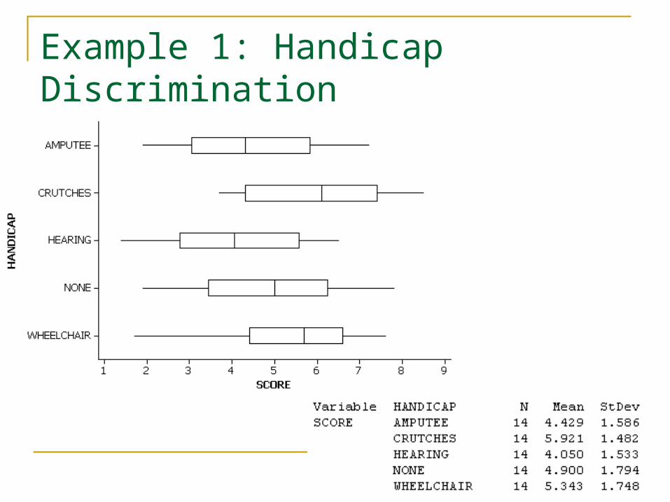
Example 1: Handicap Discrimination In 1984, handicapped individuals in the labor
force had an unemployment rate of 7% compared to 4.5% in the non-impaired labor force.
Cesare, S.J., Tannenbaum, R.J., and Dalessio, A. (1990), “Interviewers’ Decisions Related to Applicant Handicap Type and Rater Empathy,” Human Performance 3(3): 157-71.

Example 1: Handicap Discrimination Observational units?
Undergraduate students Explanatory variable
Which type of handicap in video (qualitative) Response variable
Qualification rating (quantitative) Type of study
Experiment since randomly assigned them to different videos

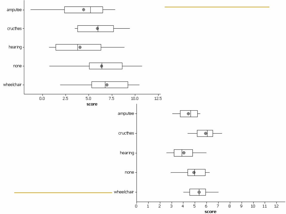
Example 1: Handicap Discrimination Is it possible that there is no treatment effect
but the observed treatment group means are 4.429, 5.921, 4.050, 4.900, 5.343?
How decide? Let i = underlying true mean treatment
response H0: none = leg amp = crutches= hearing =wheel
Ha: at least one differs
Example 1: Handicap Discrimination

Inference Procedure
Want one procedure for comparing the 5 treatment means simultaneously Take into account the distances between the
sample means relative to the variability in the data Comparisons of “between group” variability to
“within group” variability (“by chance”)

“Analysis of Variance” (ANOVA) F statistic = discrepancy in group means
variability in data
If F statistic is large, have evidence against the null hypothesis
p-value = probability of observing an F statistic at least this large when H0 is true
ErrorforSquareMean
TreatmentsforSquareMean
gN
sn
YYn
g
iii
g
iii
1
2
1
2
)1(
1) - (g

Minitab
Stat > ANOVA > One-Way

Notes
The test statistic takes the sample sizes into account, giving more weight to the group with larger sizes.
Producing a pooled estimate of the overall variability in the data requires us to assume that each population/treatment group has the same variability 2.

Checking the Technical Conditions Normal populations
Equal variances Ratio of largest SD/smallest SD < 2
Independence Random samples/randomization

Example 1: Handicap Discrimination The samples look reasonably symmetric with similar standard
deviations, so it is appropriate to apply the Analysis of Variance procedure. There is moderate evidence that the mean qualification ratings differ depending on the type of handicap (p-value = .030). Descriptively, the candidates with crutches appear to have higher ratings and the candidates with hearing impairments slightly lower ratings (other procedures could be used to follow-up to test the significance of these individual differences). This was a randomized experiment so we can attribute these differences to the handicap status but we must be cautious in thinking the students in this study are representative of a larger population, particularly, a population of employers who make hiring decisions.

Example 2: Restaurant Spending Hypotheses Technical conditions? How do different factors affect the size of the p-
value? when the population means are further apart, the p-value is
usually smaller (more evidence they aren’t equal) when the within group variability is larger, the p-value is
larger (less evidence didn’t happen by chance) when the sample sizes are larger, and there is a true
difference between the population means, then the p-value is smaller

Example 3: Follow-up Analysis Multiple comparison procedures control
overall Type I Error rate Are several different such procedures
Bonferroni, Tukey, Scheffe’… Let Minitab do all the work

Example 4: Lifetimes of Notables Which professions appear to differ?
For Thursday
Submit PP 12 in Blackboard Continue reading Ch. 12
Preview Example 5, complete (a) and (b)


