Statisticalmodelling: Theoryandpractice GillesGuillot · Stochasticsimulationandresamplingmethods...

Stochastic simulation and resampling methodsStatistical modelling: Theory and practice

Gilles Guillot

[email protected]

October 22, 2013

Gilles Guillot ([email protected]) Stochastic simulation and resampling methods October 22, 2013 1 / 32

1 Simulations, what for?

2 Pseudo uniform random number generation

3 Beyond uniform numbers on [0, 1]

4 Random number generation in R

5 An application: the bootstrap

6 Exercises


Introduction

Analysis of a stochastic model

A stochastic model involvingD: something observed (or observable) about the system (data)θ: a known or unknown parameterP (θ,D): a probability model (not necessarilly known as a nicefunction)

Three questionsOne has observed some data D, what does it say about θ? (inference)If θ is known to be equal to θ0, what does it say about D? (prediction)One has observed some data D, what does it say about future datavalue D∗? (joint inference and prediction)

Stochastic simulations used to produce some “fake data” used tounderstand/learn something about the data generating process.Much more in June course Stochastic Simulation 02443.


http://www2.imm.dtu.dk/courses/02443/

Introduction

Stochastic simulations as a tool in ordinary numericalanalysis

Integration in large dimension

Optimization and equation solving


Pseudo uniform random numbers

Pseudo uniform random number generation

Computer = most deterministic thing on earthIdea here: produce deterministic sequence that mimics randomnessMethods originate in von Neuman’s work in theoretical physics duringWWII coined “Monte Carlo” simulationsToday’s lecture:

basic idea used to produce uniform numbers in [0, 1]a statistical application: the bootstrap method



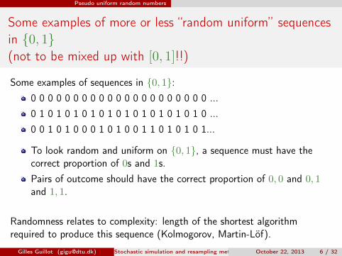
Some examples of more or less “random uniform” sequencesin {0, 1}(not to be mixed up with [0, 1]!!)

Some examples of sequences in {0, 1}:0 0 0 0 0 0 0 0 0 0 0 0 0 0 0 0 0 0 0 0 0 ...0 1 0 1 0 1 0 1 0 1 0 1 0 1 0 1 0 1 0 1 0 ...0 0 1 0 1 0 0 0 1 0 1 0 0 1 1 0 1 0 1 0 1...

To look random and uniform on {0, 1}, a sequence must have thecorrect proportion of 0s and 1s.Pairs of outcome should have the correct proportion of 0, 0 and 0, 1and 1, 1.

Randomness relates to complexity: length of the shortest algorithmrequired to produce this sequence (Kolmogorov, Martin-Löf).



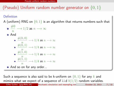
(Pseudo) Uniform random number generator on {0, 1}

DefinitionA (uniform) RNG on {0, 1} is an algorithm that returns numbers such that

#0

n−→ 1/2 as n −→∞

And#(0, 0)

n−→ 1/4 as n −→∞

#(0, 1)

n−→ 1/4 as n −→∞

#(1, 0)

n−→ 1/4 as n −→∞

#(1, 1)

n−→ 1/4 as n −→∞

And so on for any order...

Such a sequence is also said to be k-uniform on {0, 1} for any k andmimics what we expect of a sequence of i.i.d b(1/2) random variables.



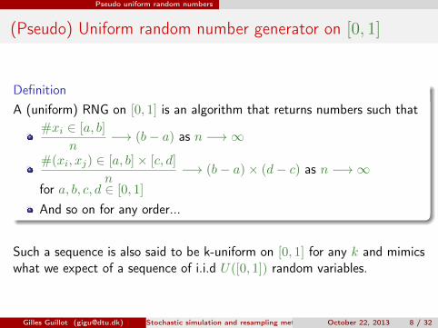
(Pseudo) Uniform random number generator on [0, 1]

DefinitionA (uniform) RNG on [0, 1] is an algorithm that returns numbers such that

#xi ∈ [a, b]

n−→ (b− a) as n −→∞

#(xi, xj) ∈ [a, b]× [c, d]

n−→ (b− a)× (d− c) as n −→∞

for a, b, c, d ∈ [0, 1]

And so on for any order...

Such a sequence is also said to be k-uniform on [0, 1] for any k and mimicswhat we expect of a sequence of i.i.d U([0, 1]) random variables.



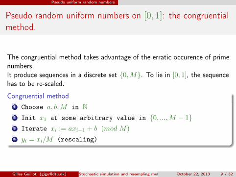
Pseudo random uniform numbers on [0, 1]: the congruentialmethod.

The congruential method takes advantage of the erratic occurence of primenumbers.It produce sequences in a discrete set {0,M}. To lie in [0, 1], the sequencehas to be re-scaled.

Congruential method1 Choose a, b,M in N2 Init x1 at some arbitrary value in {0, ...,M − 1}3 Iterate xi := axi−1 + b (mod M)

4 yi = xi/M (rescaling)



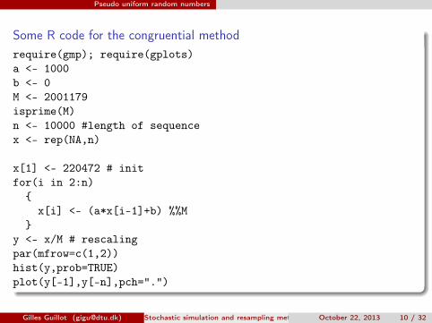
Some R code for the congruential methodrequire(gmp); require(gplots)a <- 1000b <- 0M <- 2001179isprime(M)n <- 10000 #length of sequencex <- rep(NA,n)

x[1] <- 220472 # initfor(i in 2:n)

{x[i] <- (a*x[i-1]+b) %%M

}y <- x/M # rescalingpar(mfrow=c(1,2))hist(y,prob=TRUE)plot(y[-1],y[-n],pch=".")



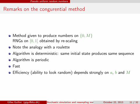
Remarks on the congurential method

Method given to produce numbers on {0,M}RNGs on [0, 1] obtained by re-scalingNote the analogy with a rouletteAlgorithm is deterministic: same initial state produces same sequenceAlgorithm is periodicFastEfficiency (ability to look random) depends strongly on a, b and M



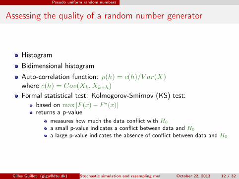
Assessing the quality of a random number generator

HistogramBidimensional histogramAuto-correlation function: ρ(h) = c(h)/V ar(X)where c(h) = Cov(Xk, Xk+h)

Formal statistical test: Kolmogorov-Smirnov (KS) test:based on max |F (x)− F ?(x)|returns a p-value

measures how much the data conflict with H0

a small p-value indicates a conflict between data and H0

a large p-value indicates the absence of conflict between data and H0



A state-of-the-art method: the Mersenne twister

Previous method in use untill late 80’sMersenne twister: algorithm proposed by Matsumoto and Nishimura in1998Iterative methodBased on a matrix linear recurrenceHas period 219937 − 1 when using 32-bit wordsName derives from the fact that period length is chosen to be aMersenne prime numberBest pseudo-RNG to dateDefault algorithm in R (cf ? RNG), Splus and Matlab


Beyond uniform numbers on [0, 1]

Simulating non-uniform random numbers

Most common families of methods include:Rejection methodsTransformation methodsMarkov chain methods


Random number generation in R

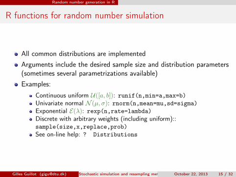
R functions for random number simulation

All common distributions are implementedArguments include the desired sample size and distribution parameters(sometimes several parametrizations available)Examples:

Continuous uniform U([a, b]): runif(n,min=a,max=b)Univariate normal N (µ, σ): rnorm(n,mean=mu,sd=sigma)Exponential E(λ): rexp(n,rate=lambda)Discrete with arbitrary weights (including uniform)::sample(size,x,replace,prob)See on-line help: ? Distributions


The bootstrap

The bootstrap


The bootstrap

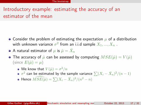
Introductory example: estimating the accuracy of anestimator of the mean

Consider the problem of estimating the expectation µ of a distributionwith unknown variance σ2 from an i.i.d sample X1, ..., Xn .A natural estimator of µ is µ = Xn

The accuracy of µ can be assessed by computing MSE(µ) = V (µ)(since E(µ) = µ)

We know that V (µ) = σ2/nσ2 can be estimated by the sample variance

∑(Xi − Xn)2/(n− 1)

Hence MSE(µ) =∑

(Xi − Xn)2/(n2 − n)


The bootstrap

Now imagine for a while that we do not know that V (µ) = σ2/n

or that σ2 =∑

(Xi − Xn)2/(n− 1)


The bootstrap

A fairly general situation:

An unknown parameter θAn estimator θNo known formula for the variance (or MSE) of θ


The bootstrap

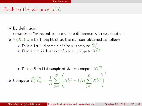
Back to the variance of µ

By definition:variance = “expected square of the difference with expectation”V (Xn) can be thought of as the number obtained as follows

Take a 1st i.i.d sample of size n, compute X(1)n

Take a 2nd i.i.d sample of size n, compute X(2)n

...

...Take a B-th i.i.d sample of size n, compute X(B)

n

Compute V (Xn) =1

B

B∑j=1

X(j)n − 1/B

B∑j=1

X(j)n

2


The bootstrap

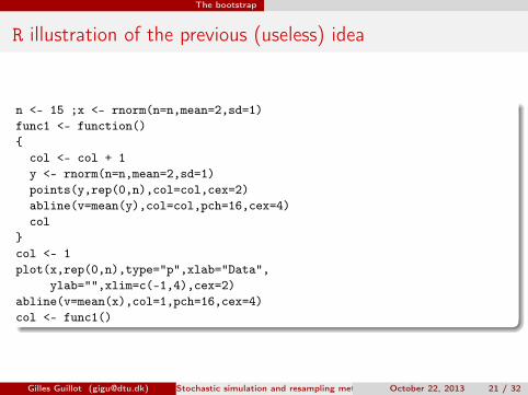
R illustration of the previous (useless) idea

n <- 15 ;x <- rnorm(n=n,mean=2,sd=1)func1 <- function(){

col <- col + 1y <- rnorm(n=n,mean=2,sd=1)points(y,rep(0,n),col=col,cex=2)abline(v=mean(y),col=col,pch=16,cex=4)col

}col <- 1plot(x,rep(0,n),type="p",xlab="Data",

ylab="",xlim=c(-1,4),cex=2)abline(v=mean(x),col=1,pch=16,cex=4)col <- func1()


The bootstrap

The previous quantity estimates V (µ) more and more accurately as Bincreases (law of large numbers)Little problem: we do not have B samples of size n, we have only one!There is a get around ... just pull your bootstraps!


The bootstrap

Estimating V (µ) with the so-called bootstrap estimator(Efron, 1979)

We have a single dataset (X1, ..., Xn)We can pretend to have B different samples of size n:

sample Y (1)1 , ..., Y

(1)n in (X1, ..., Xn) uniformly with replacement,

compute Y (1)n

sample Y (2)1 , ..., Y

(2)n in (X1, ..., Xn) uniformly with replacement,

compute Y (2)n

...

...sample Y (B)

1 , ..., Y(B)n in (X1, ..., Xn) uniformly with replacement,

compute Y (B)n

Note that Y (b)1 , ..., Y

(b)n usually have ties

Compute V (Xn) =1

B

B∑j=1

Y (j)n − 1/B

B∑j=1

Y (j)n

2


The bootstrap

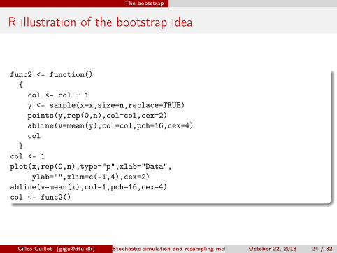
R illustration of the bootstrap idea

func2 <- function(){

col <- col + 1y <- sample(x=x,size=n,replace=TRUE)points(y,rep(0,n),col=col,cex=2)abline(v=mean(y),col=col,pch=16,cex=4)col

}col <- 1plot(x,rep(0,n),type="p",xlab="Data",

ylab="",xlim=c(-1,4),cex=2)abline(v=mean(x),col=1,pch=16,cex=4)col <- func2()


The bootstrap

Key idea underlying bootsrtap techniques:The true unknown probability distribution F of X is approximated by theempirical distribution F ∗.(Recall that F ∗ is the discrete distribution putting an equal weight 1/n oneach observed data value.)

This approximation makes sense as soon as n (sample size) is large.


The bootstrap

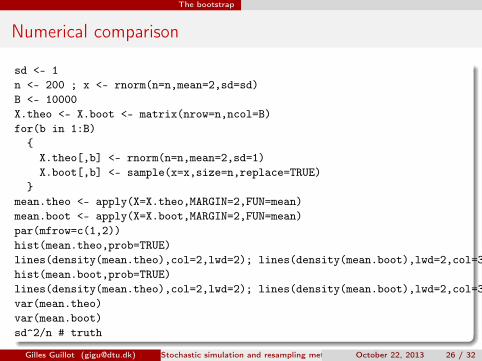
Numerical comparison

sd <- 1n <- 200 ; x <- rnorm(n=n,mean=2,sd=sd)B <- 10000X.theo <- X.boot <- matrix(nrow=n,ncol=B)for(b in 1:B)

{X.theo[,b] <- rnorm(n=n,mean=2,sd=1)X.boot[,b] <- sample(x=x,size=n,replace=TRUE)

}mean.theo <- apply(X=X.theo,MARGIN=2,FUN=mean)mean.boot <- apply(X=X.boot,MARGIN=2,FUN=mean)par(mfrow=c(1,2))hist(mean.theo,prob=TRUE)lines(density(mean.theo),col=2,lwd=2); lines(density(mean.boot),lwd=2,col=3)hist(mean.boot,prob=TRUE)lines(density(mean.theo),col=2,lwd=2); lines(density(mean.boot),lwd=2,col=3)var(mean.theo)var(mean.boot)sd^2/n # truth


The bootstrap

Summary

A collection of several samples can be mimicked by resampling thedataA theoretical parameter that can be expressed as an expectation canbe estimated by an average over the “fake” samplesThe idea is very general (see example for the median below)


The bootstrap

Bootstrap-based confidence intervals

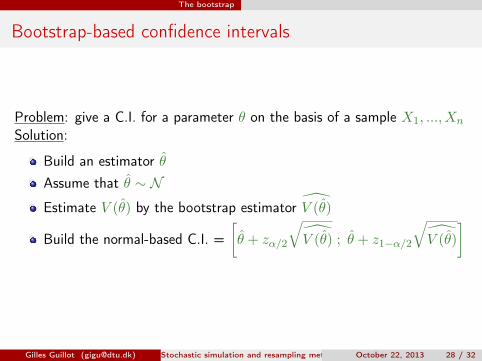
Problem: give a C.I. for a parameter θ on the basis of a sample X1, ..., Xn

Solution:

Build an estimator θAssume that θ ∼ NEstimate V (θ) by the bootstrap estimator V (θ)

Build the normal-based C.I. =[θ + zα/2

√V (θ) ; θ + z1−α/2

√V (θ)

]


The bootstrap

Take home messages

1 Stochastic simulations useful in the analyis of stat. models andordinary numerical analysis

2 Computers can produce numbers that look random3 Congruence method fast but outcome of varying quality. Default

algorithm implemented in R and Matlab highly reliable4 Lack of data can be supplemented by resampled data which involves

(simple) simulations


The bootstrap

References

Bootstrap: Chapter 8 of All of Statistics, Larry Wasserman, Springer,2004. Available on Google books.Introducing Monte Carlo Methods with R, C.P. Robert & G. CasellaSpringerlink


http://books.google.com/books?id=th3fbFI1DaMC&printsec=frontcover&dq=All+of+Statistics,+Larry+Wasserman,+Springer,+2004&hl=fr&ei=vsJpTt7_BsqSOsnzyN0F&sa=X&oi=book_result&ct=result&resnum=1&ved=0CCoQ6AEwAA#v=onepage&q=All%20of%20Statistics%2C%20Larry%20Wasserman%2C%20Springer%2C%202004&f=false

http://www.springerlink.com.globalproxy.cvt.dk/content/978-1-4419-1575-7/#section=625973&page=1

Date post:	13-Sep-2018
Category:	Documents
Upload:	phamdang
View:	215 times
Download:	0 times

Statisticalmodelling: Theoryandpractice GillesGuillot · Stochasticsimulationandresamplingmethods...

Documents