14
1 Stochastic Processes Monday, November 14, 11

1
Stochastic Processes
Monday, November 14, 11

2
Definition and Classification
X( , t): stochastic process:
X : ⌦⇥ T ! R( , t) X( , t)
where ⌦ is a sample space and T is time. {X( , t) is a family of r.v. defined on
{⌦,A,P and indexed by t 2 T .
• For a fixed 0, X(( 0, t) is a function of time or a sample function
• For a fixed t0, X(( , t0) is a random variable or a function of 2 ⌦
Discrete-time random process: n 2 T , X( , n)Continuous-time random process: t 2 TX( , n)
Monday, November 14, 11
3
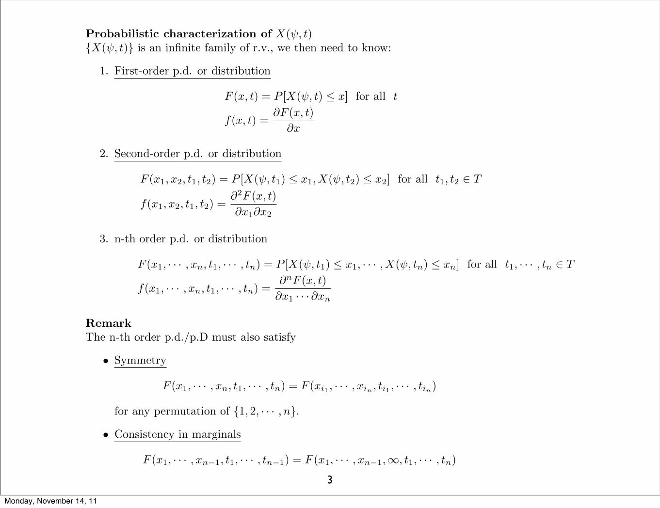
Probabilistic characterization of X( , t)
{X( , t)} is an infinite family of r.v., we then need to know:
1. First-order p.d. or distribution
F (x, t) = P [X( , t) x] for all t
f(x, t) =
@F (x, t)
@x
2. Second-order p.d. or distribution
F (x1, x2, t1, t2) = P [X( , t1) x1, X( , t2) x2] for all t1, t2 2 T
f(x1, x2, t1, t2) =@
2F (x, t)
@x1@x2
3. n-th order p.d. or distribution
F (x1, · · · , xn, t1, · · · , tn) = P [X( , t1) x1, · · · , X( , tn) xn] for all t1, · · · , tn 2 T
f(x1, · · · , xn, t1, · · · , tn) =@
nF (x, t)
@x1 · · · @xn
Remark
The n-th order p.d./p.D must also satisfy
• Symmetry
F (x1, · · · , xn, t1, · · · , tn) = F (xi1 , · · · , xin , ti1 , · · · , tin)
for any permutation of {1, 2, · · · , n}.
• Consistency in marginals
F (x1, · · · , xn�1, t1, · · · , tn�1) = F (x1, · · · , xn�1,1, t1, · · · , tn)
Monday, November 14, 11
4
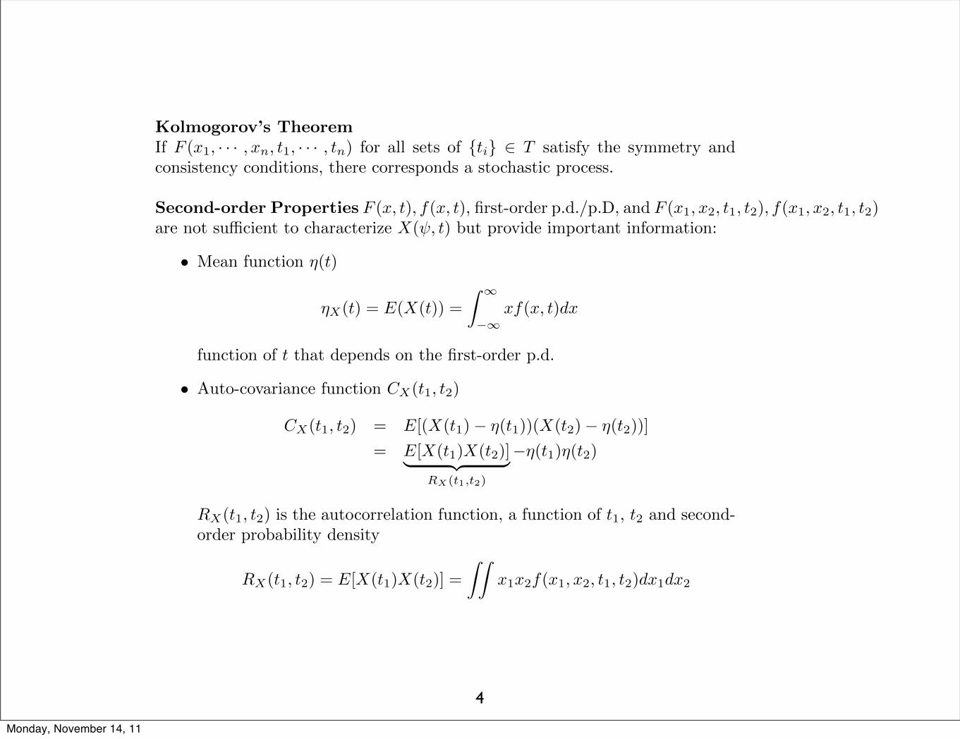
Kolmogorov’s Theorem
If F (x1, · · · , xn, t1, · · · , tn) for all sets of {ti} 2 T satisfy the symmetry and
consistency conditions, there corresponds a stochastic process.
Second-order Properties F (x, t), f(x, t), first-order p.d./p.D, and F (x1, x2, t1, t2), f(x1, x2, t1, t2)
are not su�cient to characterize X( , t) but provide important information:
• Mean function ⌘(t)
⌘X(t) = E(X(t)) =
Z 1
�1xf(x, t)dx
function of t that depends on the first-order p.d.
• Auto-covariance function CX(t1, t2)
CX(t1, t2) = E[(X(t1)� ⌘(t1))(X(t2)� ⌘(t2))]
= E[X(t1)X(t2)]| {z }RX(t1,t2)
�⌘(t1)⌘(t2)
RX(t1, t2) is the autocorrelation function, a function of t1, t2 and second-
order probability density
RX(t1, t2) = E[X(t1)X(t2)] =
ZZx1x2f(x1, x2, t1, t2)dx1dx2
Monday, November 14, 11

5
Remarks
• Note that
CX(t, t) = E[(X(t)� ⌘(t))2] = �2X(t)
or the variance of X(t).
• CX(t1, t2) relates r.v.’s at times t1 and t2, i.e., in time, while CX(t, t)relates the r.v. X(t) with itself, i.e., in space.
Correlation coe�cient
rX(t1, t2) =CX(t1, t2)
�X(t1)�X(t2)
Cross-covariance
X(t), Y (t) real processes
CXY (t1, t2) = E[(X(t1)� ⌘X(t1))(Y (t2)� ⌘Y (t2))]
= E[X(t1)Y (t2)]| {z }RXY (t1,t2)
�⌘X(t1)⌘Y (t2)
RXY (t1, t2) is the cross-correlation function.
X(t), Y (t) are uncorrelated i↵ CXY (t1, t2) = 0 for all t1 and t2 2 T .
Monday, November 14, 11
6
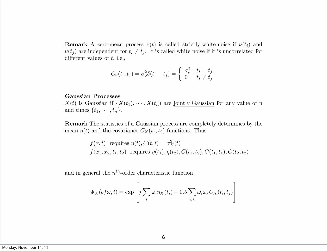
Remark A zero-mean process ⌫(t) is called strictly white noise if ⌫(ti) and
⌫(tj) are independent for ti 6= tj . It is called white noise if it is uncorrelated for
di↵erent values of t, i.e.,
C⌫(ti, tj) = �
2⌫�(ti � tj) =
⇢�
2⌫ ti = tj
0 ti 6= tj
Gaussian Processes
X(t) is Gaussian if {X(t1), · · · , X(tn) are jointly Gaussian for any value of n
and times {t1, · · · , tn}.
Remark The statistics of a Gaussian process are completely determines by the
mean ⌘(t) and the covariance CX(t1, t2) functions. Thus
f(x, t) requires ⌘(t), C(t, t) = �
2X(t)
f(x1, x2, t1, t2) requires ⌘(t1), ⌘(t2), C(t1, t2), C(t1, t1), C(t2, t2)
and in general the n
th-order characteristic function
�X(bf!, t) = exp
2
4j
X
i
!i⌘X(ti)� 0.5
X
i,k
!i!kCX(ti, tj)
3
5
Monday, November 14, 11
7
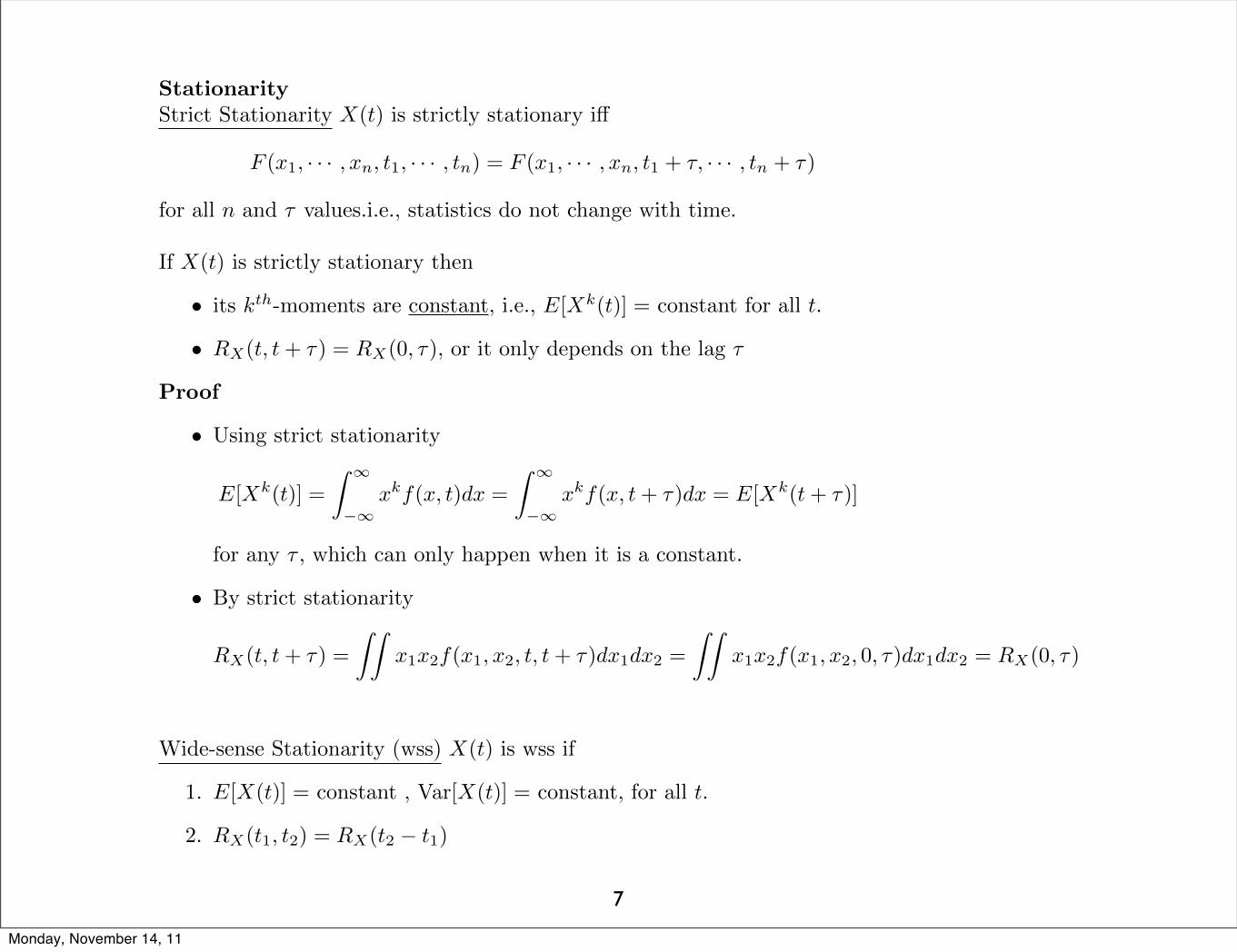
Stationarity
Strict Stationarity X(t) is strictly stationary i↵
F (x1, · · · , xn, t1, · · · , tn) = F (x1, · · · , xn, t1 + ⌧, · · · , tn + ⌧)
for all n and ⌧ values.i.e., statistics do not change with time.
If X(t) is strictly stationary then
• its k
th-moments are constant, i.e., E[X
k(t)] = constant for all t.
• RX(t, t+ ⌧) = RX(0, ⌧), or it only depends on the lag ⌧
Proof
• Using strict stationarity
E[X
k(t)] =
Z 1
�1x
kf(x, t)dx =
Z 1
�1x
kf(x, t+ ⌧)dx = E[X
k(t+ ⌧)]
for any ⌧ , which can only happen when it is a constant.
• By strict stationarity
RX(t, t+ ⌧) =
ZZx1x2f(x1, x2, t, t+ ⌧)dx1dx2 =
ZZx1x2f(x1, x2, 0, ⌧)dx1dx2 = RX(0, ⌧)
Wide-sense Stationarity (wss) X(t) is wss if
1. E[X(t)] = constant , Var[X(t)] = constant, for all t.
2. RX(t1, t2) = RX(t2 � t1)
Monday, November 14, 11
8
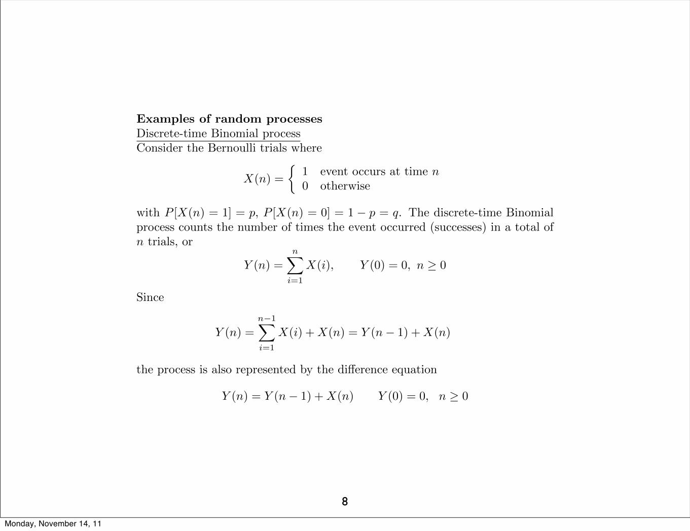
Examples of random processes
Discrete-time Binomial process
Consider the Bernoulli trials where
X(n) =
⇢1 event occurs at time n0 otherwise
with P [X(n) = 1] = p, P [X(n) = 0] = 1 � p = q. The discrete-time Binomial
process counts the number of times the event occurred (successes) in a total of
n trials, or
Y (n) =nX
i=1
X(i), Y (0) = 0, n � 0
Since
Y (n) =n�1X
i=1
X(i) +X(n) = Y (n� 1) +X(n)
the process is also represented by the di↵erence equation
Y (n) = Y (n� 1) +X(n) Y (0) = 0, n � 0
Monday, November 14, 11

9
Characterization of Y (n)First-order p.d.
f(y, n) =nX
k=0
P [Y (n) = k]�(y � k) =nX
k=0
✓n
k
◆�(y � k), 0 k n
Second and higher-order p.d. are di�cult to find given the dependence of the
Y (n)’s.Statistical averages
E[Y (n)] =
nX
i=1
E[X(i)]| {z }p
= np
Var[Y (n)] = E[(Y (n)� np)2] = E[(
nX
i=1
(X(i)� p)2]
=
X
i,j
E[(X(i)� p)(X(j)� p)] =X
i,j
E[X(i)� p]E[X(j)� p]| {z }=0 if i 6=j
independence of X(i)
=
nX
i=1
E[(X(i)� p)2]| {z }Var(X(i))=(12⇥p+0⇥q)�p2=pq
= npq
Notice that E[Y (n)] = np, so it depends on time n, and Var[Y (n)] = npq also
a function of time n, so the discrete binomial process is non-stationary.
Monday, November 14, 11

10
Random Walk Process Let the discrete binomial process be defined by Bernoulli
trials
X(n) =
⇢s event occurs at time n�s otherwise
so that
Y (n) =nX
i=1
X(i), Y (0) = 0, n � 0
Possible values at times bigger than zero
n = 1 Y (1) = �1, 1n = 2 Y (2) = 2, 0,�2
n = 3 Y (3) = �3, 1,�1, 3.
.
.
.
.
.
In general, at step n = n0 Y (n) can take values {2k � n0, 0 k n0}, so for
instance for n = 2, Y (2) can take values 2k � 2, 0 k 2 or �2, 0, 2.
Monday, November 14, 11
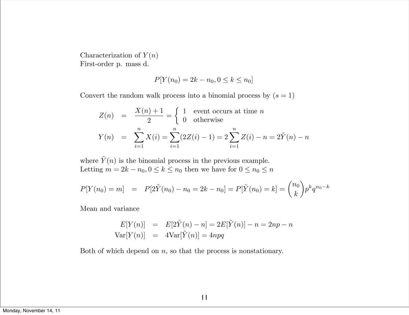
11
Characterization of Y (n)First-order p. mass d.
P [Y (n0) = 2k � n0, 0 k n0]
Convert the random walk process into a binomial process by (s = 1)
Z(n) =
X(n) + 1
2
=
⇢1 event occurs at time n0 otherwise
Y (n) =
nX
i=1
X(i) =nX
i=1
(2Z(i)� 1) = 2
nX
i=1
Z(i)� n = 2
˜Y (n)� n
where
˜Y (n) is the binomial process in the previous example.
Letting m = 2k � n0, 0 k n0 then we have for 0 n0 n
P [Y (n0) = m] = P [2
˜Y (n0)� n0 = 2k � n0] = P [
˜Y (n0) = k] =
✓n0
k
◆pkqn0�k
Mean and variance
E[Y (n)] = E[2
˜Y (n)� n] = 2E[
˜Y (n)]� n = 2np� n
Var[Y (n)] = 4Var[
˜Y (n)] = 4npq
Both of which depend on n, so that the process is nonstationary.
Monday, November 14, 11

12
Sinusoidal processes
X(t) = A cos(⌦t+ �)
A constant,frequency ⌦ and phase � are random and independent. Assume
� ⇠ U [�⇡,⇡]. The sinusoidal process X(t) is w.s.s.
E[X(t)] = AE[cos(⌦t+ �)] = AE[cos(⌦t) sin(�)� sin(⌦t) cos(�)]
= A[E[cos(⌦t)]E[sin(�)]| {z }0
�E[sin(⌦t)]E[cos(�)]| {z }0
] independence
= 0
The
E[sin(�)] =
Z ⇡
�⇡
1
2⇡sin(�)d� = 0
area under a period of the sinusoid T0 = 2⇡, likewise for E[cos(�)] = 0.
The autocorrelation
RX(t+ ⌧, t) = E[X(t+ ⌧)X(t)] = A2E[cos(⌦(t+ ⌧) + �) cos(⌦t+ �)]
=
A2
2
E[cos(⌦⌧) + cos(2⌦t+ ⌦⌧ + 2�)]
=
A2
2
E[cos(⌦⌧)] +
⇢A2
2
E[cos(2⌦t+ ⌦⌧) sin(2�)]� A2
2
E[sin(2⌦t+ ⌦⌧) cos(2�)]
�
| {z }0
=
A2
2
E[cos(⌦⌧)]
where the zero term is obtained because of the independence and that the ex-
pected values E[sin(2�)] = E[cos(2�)] = 0 by similar reasons as above.
Monday, November 14, 11

13
X(t) = A cos(!0t), A ⇠ U [0, 1], !0 constant. X(t) is non-stationary.
t X(t)0 A cos(0) = A ⇠ U [0, 1]
⇡4!0
A cos(
⇡/4) =
Ap2
2 ⇠ U [0,p2/2]
⇡!
o
�A ⇠ U [�1, 0]
For each time the first-order p.d. is di↵erent so the process is not strictly
stationary. The process can be shown not to be wide-sense stationary:
E[X(t)] = cos(!0t)E[A] = 0.5 cos(!0t)
RX(t+ ⌧, t) = E[A2] cos(!0(t+ ⌧)) cos(!0t)
= �2A[cos(!0⌧) + cos(!0(2t+ ⌧))]
RX(t, t) = Var[X(t)] = �2A(1 + cos(2!0t)
which gives that the mean and the variance are not constant, and the auto-
correlation is not a function of the lag, therefore the systems is not wide-sense
stationary.
Monday, November 14, 11
14
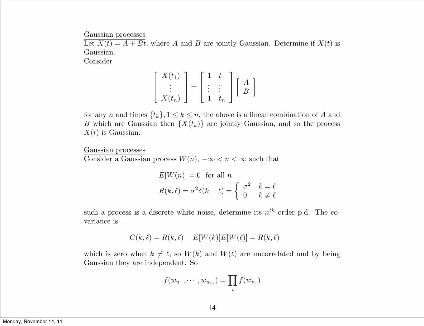
Gaussian processes
Let X(t) = A+ Bt, where A and B are jointly Gaussian. Determine if X(t) isGaussian.
Consider
2
64X(t1)
.
.
.
X(tn)
3
75 =
2
641 t1.
.
.
.
.
.
1 tn
3
75
AB
�
for any n and times {tk}, 1 k n, the above is a linear combination of A and
B which are Gaussian then {X(tk)} are jointly Gaussian, and so the process
X(t) is Gaussian.
Gaussian processes
Consider a Gaussian process W (n), �1 < n < 1 such that
E[W (n)] = 0 for all n
R(k, `) = �2�(k � `) =
⇢�2 k = `0 k 6= `
such a process is a discrete white noise, determine its nth-order p.d. The co-
variance is
C(k, `) = R(k, `)� E[W (k)]E[W (`)] = R(k, `)
which is zero when k 6= `, so W (k) and W (`) are uncorrelated and by being
Gaussian they are independent. So
f(wn1 , · · · , wnm) =
Y
i
f(wni)
Monday, November 14, 11


