125


Studies and reports in hydrology 29

Recent titles in this series
20. Hydrological maps . Co-édition Unesco-WMO. 21 * World catalogue of very large floods/Répertoire mondial des très fortes crues. 22. Floodflow computation. Methods compiled from world experience. 23. Water quality surveys. 24. Effects of urbanization and industrialization on the hydrological regime and on water quality. Proceedings
of the Amsterdam Symposium, October 1977/Effets de l'urbanisation et de l'industrialisation sur le régime hydrologique et sur la qualité de l'eau. Actes du Colloque d'Amsterdam, octobre 1977. Co-edition IAHS-Unesco/Coédition AISH-Unesco.
25. World water balance and water resources of the earth. (English edition). 26. Impact of urbanization and industrialization on water resources planning and management. 27. Socio-economic aspects of urban hydrology. 28. Casebook of methods of computation of quantitative changes in the hydrological régime of river basins due to human
activities 29. Surface water and groundwater interaction.
* Quadrilingual publication : English — French — Spanish — Russian.
For details of the complete series please see the list printed at the end of this work.
Surface water and groundwater interaction
A contribution to the International Hydrological Programme
Report prepared by the International Commission on Groundwater
Edited by C . E . Wright
lunssco

The designations employed and the presentation of material throughout the publication do not imply the expression of any opinion whatsoever on the part of Unesco concerning the legal status of any country, territory, city or area or of its authorities, or concerning the delimitation of its frontiers or boundaries.
Published, in 1980 by the United Nations Educational, Scientific and Cultural Organization 7 place de Fontenoy, 75700 Paris
Printed by Imprimerie de la Manutention, Mayenne
I S B N 92-3-101862-0
O Unesco 1980
Primed in France
Preface
The "Studies and Reports in Hydrology" series, like the related collection of "Technical Papers in Hydrology", was started in 1965 when the International Hydrological Decade ( I H D ) was launched by the General Conference of Unesco at its thirteenth session. The aim of this undertaking was to promote hydrological science through the development of international co-operation and the training of specialists and technicians.
Population growth and industrial and agricultural development are leading to constantly increasing demands for water, hence all countries are endeavouring to improve the evaluation of their water resources and to m a k e more rational use of them. The I H D was instrumental in promoting this general effort. W h e n the Decade ended in 1974, I H D National Committees had been formed in 107 of Unesco's 135 M e m b e r States to carry out national activities and participate in regional and international activities within the I H D programme.
Unesco was conscious of the need to continue the efforts initiated during the International Hydrological Decade and, following the recommendations of M e m b e r States, the Organization decided at its seventeenth session to launch a new long-term intergovernmental programme, the International Hydrological Programme (IHP), to follow the decade. The basic objectives of the I H P were defined as follows: (a) to provide a scientific framevork for the general development of hydrological activities ; (b) to improve the study of the hydro-logical cycle and the scientific methodology for the assessment
of water resources throughout the world, thus contributing to their rational use; (c) to evaluate the influence of man's activities on the water cycle, considered in relation to environmental conditions as a whole; (d) to promote the exchange of information on hydrological research and on new developments in hydrology; (e) to promote education and training in hydrology; (f) to assist M e m b e r States in the organization and development of their national hydrological activities.
The International Hydrological Programme became operational on 1 January 1975 and is to be executed through successive phases of six years' duration. I H P activities are co-ordinated at the international level by an intergovernmental council composed of thirty M e m b e r States. The members are periodically elected by the General Conference and their representatives are chosen by national committees.
The purpose of the continuing series "Studies and Reports in Hydrology" is to present data collected and the main results of hydrological studies undertaken within the framework of the decade and the new International Hydrological Programme, as well as to provide information on the hydrological research techniques used. The proceedings of symposia will also be included. It is hoped that these volumes will furnish material of both practical and theoretical interest to hydrologists and governments and meet the needs of technicians and scientists concerned with water problems in all countries.

Contents
1. INTRODUCTION 11
1.1 Purpose and Scope of the Report 11
1.2 Formation and Activity of the Working Group 12
1.3 Relationship with other IHP Working Groups 13
2. DEFINITION OF THE INTERACTION I4
2.1 Part of Hydrological Cycle Considered 14
2.2 Recharge of Groundwater 15
2.2.1 Recharge by Precipitation 15
2.2.2 Recharge by Rivers and Canals 17
2.2.3 Recharge by Lakes 19
2.2.4 Artificial Recharge 20
2.3 Groundwater Component of River Flow 20
2.4 Influence of the Interaction on Water Quality 22
2.4.1 Surface Water to Groundwater 23
2.4.2 Groundwater to Surface Water 25
3. METHODS OF ASSESSING THE INTERACTION 27
3.1' Channel Water Balance 27
3.1.1 Compilation for River Reaches 28
3.1.2 Equations for River Reaches 28
3.1.3 Compilation for River Systems 29
3.1.4 Equations for River Systems 29
3.1.5 Computation of the Elements 30
3.1.5.1 Exchange Between Rivers and Aquifers 31
3.1.5.2 River Flow, Intermediate Inflow, Abstractions and Returned Water 32
3.1.5.3 Channel Regulation 32
3.1.5.4 Precipitation 32
3.1.5.5 Evaporation from Surface Water 32
3.1.5.6 Change of Stored Moisture 33
3.1.5.7 Ice Formation and Melting 33

3.1.5.8 Areal Definition of Flood Plain Reaches 33
3.2 Hydrograph Analysis 33
3.2.1 Flow Separation 33
3.2.2 Graphic Separation of River Hydrograph 36
3.2.3 Recession Curve for River Hydrograph Separation 39
3.3 Groundwater Table Fluctuations 41
3.3.1 Temperate Areas 42
3.3.2 Arid Areas 47
3.4 Use of Isotopes as Tracers 50
3.4.1 Introduction 50
3.4.2 Stable Isotopic Composition of Natural Waters 51
3.4.3 Environmental Tritium Concentration of Natural Waters 52
3.4.4 Recharge of Groundwater by Rivers 53
3.4.5 Recharge of Groundwater by Lakes 57
3.4.6 Groundwater to Surface Water 58
3.5 Use of Mathematical Models 59
3.5.1 Purpose of Modelling 59
3.5.2 Groundwater Recharge 60
3.5.3 Spring-Aquifer Interaction 61
3.5.4 Rivers and Canals 62
3.5.5 Lake-Aquifer Interaction 65
3.5.6 Example of Finite Element Analysis 66
3.5.7 Rainfall-Runoff Models 69
4. ACCURACY OF METHODS OF ASSESSMENT 74
4.1 Surface Water Flow 74
4.1.1 Temperate Areas 75
4.1.2 Arid and Semi-arid Areas 77
4.1.2.1 Measurement of Flood Flows 79
4.1.2.2 Measurement of Low Flows 80
4.2 Aquifer Characteristics 81
4.2.1 Hydraulic Conductivity 82
4.2.1.1 Laboratory Determination of Hydraulic Conductivity 82
4.2.1.2 Field Determination of Hydraulic Conductivity 82
4.2.2 Transmissivity 83
4.2.3 Specific Yield 84
4.2.4 Coefficient of Storage 84
4.2.5 Infiltration 86
4.3 Relative Accuracy of the Methods of Assessment 86
4.3.1 Channel Water Balance 87
4.3.2 Flow Separation 88
4.3.3 Mathematical Models 89

5. CASE STUDIES 93
5.1 Temperate Area: Great Ouse Pilot Scheme, UK 93
5.1.1 Introduction 93
5.1.2 Description of the Pilot Scheme Area 94
5.1.3 Measurements 97
5.1.4 Natural River Flow and Groundwater Level Relationship 98
5.1.5 Analysis of Group Pumping Tests, 1971 101
5.2 Temperate Area: The Moscow Artesian Basin, USSR 102
5.2.1 Introduction 102
5.2.2 The Moscow Basin 102
5.2.3 Analyses 103
5.2.4 Future Situation 104
5.3 Arid Area with Irrigation: Chu Valley, USSR 106
5.3.1 Introduction 106
5.3.2 The River Chu 106
5.3.3 Description of the Study Reaches 106
5.3.4 The Channel Water Balance 107
5.3.5 Summary 107
5.4 Arid Area: Groundwater Replenishment by Surface Water, Tunisia 109
5.4.1 Introduction 109
5.4.2 Aguifer Recharge in' the Kairouan Plain 109
5.4.3 Recharge by Surface Runoff from the Zeroud Wadi 109
6. CONCLUDING REMARKS AND RECOMMENDATIONS 113
6.1 Concluding Remarks 113
6.2 Recommendations 115
REFERENCES 116
SELECTED PAPERS FROM 1979 SYMPOSIA 123

Intvoäuation
i. Introduction 1.1 Purpose and Scope of the Report
There has been a tendency in past years for separate departments to develop specialising in
either surface water or groundwater systems. For this reason the understanding of the inter
action between surface water and groundwater and techniques for its analysis have tended to be
less well advanced than those for either discipline. In recent years the traditional division
between the disciplines has tended to be reduced with the result that some useful advances have
been made in understanding the interaction between surface water and groundwater. This report
does not attempt to review all the relevant research of recent years but rather to emphasise
and illustrate the importance of the subject.
Improvements in understanding the interaction can provide information useful in the
management of water resources. For example existing schemes may be operated more efficiently
and new techniques may be considered in planning the future development of resources. In all
areas where water is a relatively scarce commodity there is a positive requirement to define
the interaction accurately. One of the main purposes of this report is to assist developing
countries, especially those in arid areas, in the management of their water resources.
However, there are likely to be benefits arising as a result of accurately defining the inter
action in other regions such as those where the demand for water represents a high proportion
of the total resource and where changes in the interaction caused by man have a marked
beneficial or detrimental effect.
Detailed consideration has been confined to one part of the hydrological cycle, the
interaction between surface water and groundwater. In temperate regions the main aspect of
this process is the flow of groundwater to rivers, and in arid regions the flow is frequently
in the reverse direction with surface runoff recharging groundwater. Subject areas covered by
other Working Groups such as irrigation, groundwater models, water quality and low river flows
are referred to but not covered in detail. For example the effect of irrigation is included
in a case study, and sections of the report contain a discussion of groundwater models and
water quality. Changes in water quality due to the effect of man in polluting either surface
water or groundwater is a major topic that is referred to only briefly. Methods of assessing
the interaction between surface water and groundwater are described together with an
11

Introduction
assessment of their accuracy. Four case studies are included. Two describe investigations in
temperate regions and two describe aspects of the interaction process in arid regions.
Publications referred to in the text are listed in the references and an additional list of
selected relevant papers is given from symposia held during 1979 at Dortmund (FRG), Vilnius
(USSR) and Canberra (Australia).
1.2 Formation and Activity of the Working Group
The second session of the Intergovernmental Council of the International Hydrological
Programme (IHP), was held in June 1977, when the decision was taken to:
invite the Secretariat in co-operation with the International Commission on
Ground Water (ICGW) of the International Association for Hydrological
Sciences (IAHS). to prepare a technical report 'Improvement of methods of
assessment of the interaction between groundwater and river flow' and
report on the progress of this project to the third session of the Council.
Two sessions of the Working Group have been organised by the ICGW Secretary with the
assistance of the IHP Secretariat of Unesco. The first session was held at the Unesco
headquarters in Paris from 12 to 16 June 1978 and the second was held at Dortmund from 7 to
11 May 1979. The Working Group was composed as follows.
First Session Second Session
Mr V V Kuprianov (USSR) Mr 0 V Popov (USSR)
Mr J Soveri (Finland) Mr J Soveri (Finland)
Mr C E Wright (Chairman, UK) Mr C E Wright (Chairman, UK)
Mr H Zebidi (Tunisia) Mr M Ennabli (Tunisia)
In addition the following experts were invited to attend the sessions :
First Session Second Session
Mrs N Kapotova (USSR)
Mr C Pollett (Australia)
Mr J A Rodier
Mr G Castany
Mr M G Bos
(IAHS)
(IAH)
(ICID Committee on Irrigation Efficiencies)
The report has been prepared by the members of the Working Group together with the following
invited authors :
Mr C van den Akker (Netherlands)
Mr D A Kraijenhoff van de Leur (Netherlands)
Mr B R Payne (IAEA)
Mr J A Rodier (France)
Mr K R Rushton (UK)
12

Introduction
Mr H J Colenbrander, Mr C E Wright and Mr Y N Bogoyavlensky were responsible for the final
editing.
1.3 Relationship with other IHP Working Groups
Parts of the subject area of this report could overlap or are closely linked to the work of
other IHP Working Groups. The subjects associated with these Working Groups are listed to
enable further information to be obtained if required.
Project 5.1 Assessment of quantitative changes in the hydrological regime of river basins
due to human activities (1975-1980) - Preparation of a casebook on methods of
computation (1975-1979).
Project 5.4 Investigation of water regime of river basins affected by irrigation (1975-1980)
Preparation of a technical report (1978-1980).
Project 7.3 Investigations of processes of quality and quantity changes of groundwater
resources due to urban and industrial development.
Project 8.1 Physical and mathematical models for investigation and predicting the changes in
groundwater regimes due to human activities.
Project 8.2 Study of groundwater recharge, including water quality aspects.
Part of the terms of reference for project 7.3 include a review of the present knowledge
of the interaction between surface water and groundwater in the urban environment. Therefore
this report (project 3.6) does not include a section on the urban environment.
13

Definition of the Interaction
2. Definition of the interaction 2.1 Part of Hydrological Cycle Considered
The interaction between surface water and groundwater is a part of the hydrological cycle that
has been examined in some detail in recent years. There are two main aspects of this process,
firstly the flow of groundwater to support river flow and secondly the flow from rivers to
groundwater. The former is a common occurrence in temperate regions whereas the latter occurs
widely in arid regions. Figure 1 is a simplified conceptual model that illustrates the subject
area of this report. There is considerable scope for modifying the figure to allow for
local conditions. For example in highly permeable areas the surface storage component could
be negligible and therefore be omitted.
poration
Capillar
Rise
Precipitation
1 Surface
Storage
< Infiltratior
Storage in
Unsaturated Zone
i
i
1
Groundw
Rechar
Groundwater
Storage
ater
ge
Overland flow
Interflow
Base flow
<
Direct
Runoff
Total
Runoff
Figure 1 A conceptual model
River flow is derived essentially from precipitation less evaporation and the routes by
which precipitation becomes river flow are shown in Figure 1. In a natural river system with
14

definition of the Interaction
negligible abstractions and discharges there are two main components of river flow, namely
direct runoff and base flow. Direct runoff may be subdivided into channel precipitation,
overland flow and interflow, whereas base flow is that part of river flow that is derived from
groundwater. Groundwater flow is defined as flow within the saturated zone. In catchments
with more than one aquifer the base flow component may be subdivided according to the
contributing formation. The proportion of' direct runoff or base flow in total river flow may
vary substantially from one basin to another and from month to month because of the effect of
different soil types, geology, land use, topography, stream patterns and changes in
precipitation, evaporation and temperature.
In temperate regions groundwater recharge is derived mainly from precipitation less
evaporation, where evaporation is defined as including transpiration and interception losses
from vegetation. However, in arid regions, where annual potential evaporation exceeds
precipitation, groundwater recharge is frequently derived from temporary rivers that are in
flood. More generally both flood water and base flow from mountain rivers can recharge
aquifers in the foothills and adjacent relatively dry low lying areas. In addition groundwater
recharge may occur from lakes, canals and excess irrigation. If the groundwater table is near
to the surface of the ground, then the capillary rise may enable evaporation to deplete
directly the groundwater storage. The infiltration process and the movement of water in the
unsaturated zone are not discussed in detail in this report.
The storage, flow and quality characteristics of surface water and groundwater are
frequently dissimilar. For this reason the interaction is important in water-resource
development since advantage may be taken of the differing characteristics to increase yields or
improve the quality of water supplies. Changes in one part of the hydrological cycle may
induce beneficial or detrimental changes in another part of the cycle. A definition of the
water balance and its elements or component parts has been given by Brown et aZ.t (1972) .
2.2 Recharge of Groundwater
2.2.1 Recharge by Precipitation
The main source of groundwater recharge is generally directly from precipitation particularly
in those areas where annual average precipitation exceeds potential evaporation. Evaporation
may deplete water held in surface storage, in the soil or in the aquifer as shown in Figure 1.
Groundwater recharge occurs when the residual precipitation (precipitation less actual
evaporation) has infiltrated to the groundwater table. This may occur from several hours to
several months after the precipitation event. If the precipitation is in the form of snow then
infiltration is delayed indefinitely until there is a thaw.
To fully understand the characteristics of aquifer storage it is necessary to investigate
the characteristics of precipitation, evaporation, temperature and the unsaturated zone which
collectively determine the temporal distribution and rate of recharge. In some parts of
western Europe, consecutive monthly totals of precipitation may be regarded as independent
(random) events that are uncorrelated with past or future monthly totals, whereas evaporation
has a strong seasonal (cyclic) pattern that is repeated year after year. In such areas
15
Definition of the Interaction
significant random and cyclic components are observed in time-series recharge data. Where
precipitation and evaporation data display different properties the characteristics of recharge
data will vary accordingly and in colder regions will be significantly influenced by temp
erature as discussed in section 3.3.
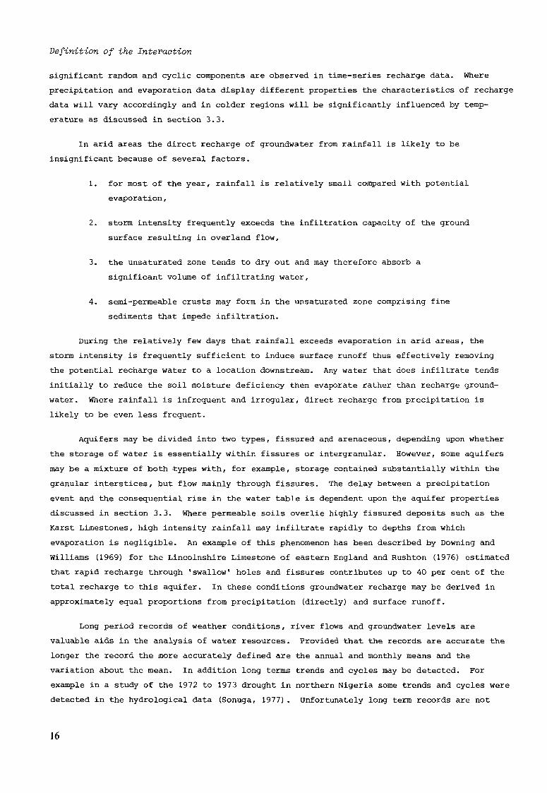
In arid areas the direct recharge of groundwater from rainfall is likely to be
insignificant because of several factors.
1. for most of the year, rainfall is relatively small compared with potential
evaporation,
2. storm intensity frequently exceeds the infiltration capacity of the ground
surface resulting in overland flow,
3. the unsaturated zone tends to dry out and may therefore absorb a
significant volume of infiltrating water,
4. semi-permeable crusts may form in the unsaturated zone comprising fine
sediments that impede infiltration.
During the relatively few days that rainfall exceeds evaporation in arid areas, the
storm intensity is frequently sufficient to induce surface runoff thus effectively removing
the potential recharge water to a location downstream. Any water that does infiltrate tends
initially to reduce the soil moisture deficiency then evaporate rather than recharge ground
water. Where rainfall is infrequent and irregular, direct recharge from precipitation is
likely to be even less frequent.
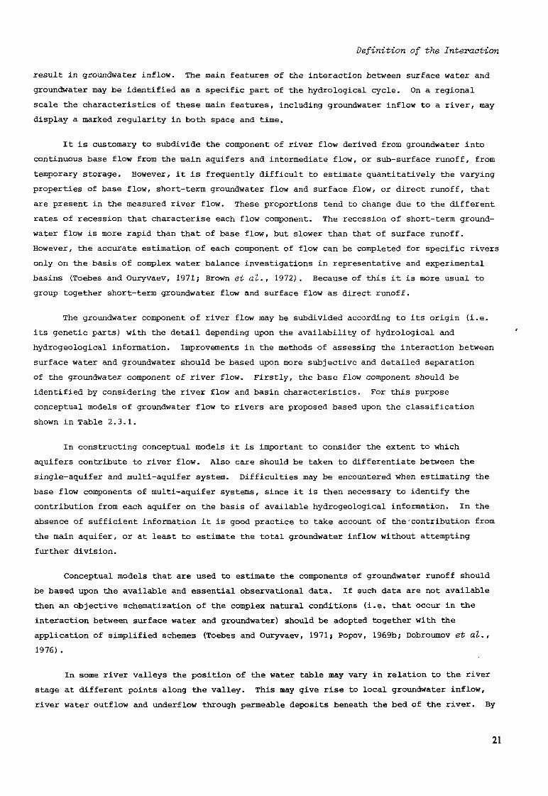
Aquifers may be divided into two types, fissured and arenaceous, depending upon whether
the storage of water is essentially within fissures or intergranular. However, some aquifers
may be a mixture of both types with, for example, storage contained substantially within the
granular interstices, but flow mainly through fissures. The delay between a precipitation
event and the consequential rise in the water table is dependent upon the aquifer properties
discussed in section 3.3. Where permeable soils overlie highly fissured deposits such as the
Karst Limestones, high intensity rainfall may infiltrate rapidly to depths from which
evaporation is negligible. An example of this phenomenon has been described by Downing and
Williams (1969) for the Lincolnshire Limestone of eastern England and Rushton (1976) estimated
that rapid recharge through 'swallow' holes and fissures contributes up to 40 per cent of the
total recharge to this aquifer. In these conditions groundwater recharge may be derived in
approximately equal proportions from precipitation (directly) and surface runoff.
Long period records of weather conditions, river flows and groundwater levels are
valuable aids in the analysis of water resources. Provided that the records are accurate the
longer the record the more accurately defined are the annual and monthly means and the
variation about the mean. In addition long terms trends and cycles may be detected. For
example in a study of the 1972 to 1973 drought in northern Nigeria some trends and cycles were
detected in the hydrological data (Sonuga, 1977) . Unfortunately long term records are not
16

Definition of the Interaction
available in many areas and the assessment of rainfall characteristics may be complicated by a
high variability of daily, monthly and annual rainfall within relatively small areas (Balek,
1978) .
Where long period weather records exist and a suitable model is available, it may be
possible to synthesise long sequences of aquifer recharge data. An abstract from such a
synthesised record is shown in Table 2.2.1 (Morel and Wright, 1978) which illustrates the
random and seasonal components of aquifer recharge for the Chalk of eastern England (West
Suffolk). This area has an annual average rainfall of 600 mm of which 450 mm is evaporated.
Recharge occurs mainly during the four months December to March, but may be negligible if
winter rainfall is insufficient to restore the soil to field capacity. The exceptionally dry
weather of 1972-73 and 1975-76 resulted in negligible groundwater recharge for periods of
18 months. From the long synthesised record it is apparent that such events may occur in this
area on average three or four times every 100 years.
Table 2.2.1 Typical values of monthly aquifer recharge in eastern England (1965-76)
(millimetres)
Year
1965
1966
1967
1968
1969
1970
1971
1972
1973
1974
1975
1976
Jan
0
20
23
39
57
49
70
51
0
0
54
0
Feb
0
54
36
22
49
50
10
30
0
46
13
0
Mar
12
0
0
1
37
23
23
24
0
2
64
0
Apr
10
9
12
0
0
29
0
0
0
0
22
0
May
0
0
21
0
20
0
0
0
0
0
0
0
Jun
0
0
0
0
0
0
0
0
0
0
0
0
Jul
0
0
0
0
0
0
0
0
0
0
0
0
Aug
0
0
0
13
0
0
0
0
0
0
0
0
Sep
0
0
0
56
0
0
0
0
0
0
0
0
Oct
0
0
0
24
0
0
0
0
0
0
0
0
Nov
24
24
0
28
0
0
2
0
0
88
0
0
Dec
91
67
40
42
0
0
15
0
0
21
0
17
Total
137
174
132
225
163
151
120
105
0
157
153
17
2.2.2 Recharge by Rivers and Canals
Recharge may occur whenever the stage in a river or canal is above that of the adjacent ground
water table, provided that the bed comprises permeable or semi-permeable material. This type
of groundwater recharge may be temporary, seasonal or continuous. Also it may be a natural
phenomenon or induced by man. For example intermittent recharge may occur in arid regions
when temporary rivers are flowing in valleys that are usually dry (Besbes et al., 1978),
seasonal flow can occur to and from bank storage (Popov, 1969), and there may be a
continuous flow to groundwater from rivers and canals (Smiles and Knight, 1979). In New
Zealand several groundwater bodies near the coast are recharged mainly by seepage from river
beds, and it is probable that similar processes occur in other places around the world
(Woudt et al., 1979). When there is seepage from a canal or ditch overlying a shallow water
17

Definition of the Interaction
table, water-logging of the soil at points some distance from the canal is a distinct
possibility (Bruch, 1979).
Man can induce groundwater recharge from rivers by lowering the water table adjacent to
rivers or by raising the river stage. The former is a relatively common occurrence which may
be caused by groundwater abstractions for supply or by mine drainage, and the latter may be
caused by reservoir releases (Kemp and Wright, 1977), weirs or other engineering works. A
serious deterioration in groundwater quality may result if the recharge water is saline or
significantly polluted. This is discussed in section 2.4.
Since the replenishment of groundwater by temporary rivers is frequently the main source
of aquifer recharge in arid regions, much of this section describes the process in such areas
and additional information is contained in two case studies. However, groundwater recharge
from rivers also occurs in other regions where the geological conditions are favourable,
especially where there are Karstic rocks.
In arid areas groundwater recharge from precipitation is generally limited because of
high rates of potential evaporation and other factors described in section 2.2.1. On the other
hand the replenishment of groundwater by rivers in flood is frequently the major source of
recharge. Temporary rivers are formed in the valleys, or wadis, following intense storms in
the hills which are sufficiently severe to generate surface runoff. These temporary rivers
may terminate either in spreading zones where the flood water infiltrates to the aquifer below,
or in chotts or sebkhats which are low lying areas where temporary lakes are formed. Water
that accumulates in these depressions evaporates leaving behind its salt content. In both
cases the aquifers are recharged mainly in the foothills, or piedmont zones, where the
surface runoff is concentrated and where topographical conditions and soil permeability tend
to be more favourable for infiltration to the saturated zone.
Several factors combine to enable recharge to take place in the piedmont zones:
1. in such areas there is a thickness of permeable detritus comprising sand,
gravel and talus (detritus fallen from a cliff face),
2. the beds of the wadis are higher than the groundwater table,
3. water may flow horizontally through the banks,
4. the surface water spreads out over the ground thus accelerating the process
of infiltration and subsoil saturation,
5. the finer sediments that could impede infiltration are carried to the
downstream periphery of the recharge zone.
Groundwater recharge from temporary rivers is very irregular in both time and space,
just like the storms that produce it. In contrast to direct recharge from precipitation it is
relatively localised and concentrated with a rapid and divergent groundwater flow at the
point where the valleys open out into the plain. After each flood event there is a period
18

Definition of the Interaction
during which the aquifer is recharged causing a rise in the water table in that area. The
observed changes in the piezometric surface are the result of the superimposition of the
recent and previous flood events, so that the effect of recharge from a specific flood is
superimposed upon the preceding recession of the water table.
The rise in groundwater levels is related to the size of the flood. However, there is a
delay in the response of the water table due to two factors. Firstly there is a delay due to
the thickness, permeability and porosity of the unsaturated zone, and secondly the horizontal
propagation of the flood wave in the saturated zone is related to the diffusivity of the
aquifer.
A recession of groundwater levels follows the rise caused by infiltrating flood water.
When flow through the unsaturated zone ceases, there is a recession in groundwater levels
until such time as the next major recharge episode. In areas close to the wadis the variabil
ity of inflows may be sufficient to prevent groundwater flow from reaching the steady state
condition, and the effect of major floods may be apparent even after several months. Further
away from the recharge zone the amplitude of groundwater level fluctuations decreases and the
flow approximates to or reaches a steady state condition.
In areas where aquifers are recharged by rivers or canals, the safe groundwater yield
(Q) may be expressed as (Bochever, 1979) :
Q = Q e + Q± 2.2(1)
where Q is that part of the yield derived from natural groundwater sources and Q. is the total
inflow from other sources such as rivers. The determination of Q. is dependent primarily upon
analyses of the interaction between groundwater and river water.
2.2.3 Recharge by Lakes
In the United States a large number of small reservoirs are being built and small lakes are
increasingly being used as a focal point in urban planning. This has given rise to pollution
and amenity problems that for their solution require some understanding of lake hydrology of
which the interaction between lakes and groundwater is an integral part (Cherkauer, 1977) .
In many studies of lake hydrology the precipitation, evaporation and inflow/outflow data
are available. However, evaporation assumptions in particular may lead to errors in the water
balance. If the residual is allocated to groundwater effects then serious misunderstandings
could arise concerning the interaction of lakes and groundwater. To investigate this inter
action, numerical model simulations were carried out (Winter, 1976).
Most natural lakes in the United States are caused by glaciation, and the studies by
Winter (1976) apply especially to those conditions. The lines separating the various types of
flow system, or divide, were obtained for various situations. In each case the groundwater
levels surrounding the lake were assumed to be at a higher level than the lake surface, and a
point was located on the divide where the head is a minimum. This minimum head may occur
19

Definition of the Interaction
beneath the shoreline on the downstream side of the lake and is called the stagnation point.
The relationship of the head at the stagnation point to the lake level is fundamental to
understanding the interaction of lakes and groundwater. If the head at the stagnation point
is greater than the lake level it is impossible for water to move from the lake to groundwater.
If a stagnation point is located then the divide is continuous, the lake cannot leak, and it
is the discharge point for the groundwater flow system. Alternatively if there is no stag
nation point then the lake can leak through part or all of its bed.
2.2.4 Artificial Recharge
To increase the natural replenishment of aquifers, man has used artificial recharge in
addition to those methods described in section 2.2.2 (rivers and canals). Natural infiltration
may be augmented in two ways. The first is through surface works, including recharge lagoons,
ditches, the building of low dams to cause flooding of riverside tracts, and excess irrigation.
These methods are, as with natural infiltration subject to evaporation losses and may occupy
large areas of land. The second means of augmentation is to inject the recharge water directly
into the aquifer through shafts and boreholes. While this method avoids evaporation losses and
reduces land use, there is the disadvantage that recharge water often requires extensive
treatment before injection to avoid serious clogging of the recharge wells. The normal source
of recharge water is surface runoff, but treated effluents and cooling water have been used.
Artificial recharge dates from early in the nineteenth century in Europe and near the
end of that century in the United States. More recently the experience in the United States
has been summarised by Todd (.1960) , in Israel by Harpaz (1970) and in the United Kingdom by
Rodda et dl., (1976). In arid and semi-arid regions, such as parts of the western United
States, salinity increases have been observed in both groundwater and surface water due to the
effects of irrigation practices. Much of the irrigation water is lost by evaporation, but some
recharges the aquifers and provides an increment to river flow. In these areas the
concentration of dissolved solids tends to increase and may reach a level intolerable to many
crops. In several places this effect is so pronounced that the quality of water rather than
the amount available restricts water use. This has led to the development of computer models
to predict changes in dissolved solid concentrations in response to varying hydrologie stresses
(Konikow and Bredehoeft, 1974).
The effect of excess irrigation upon aquifer recharge is such an important issue in arid
and semi-arid climates that a case study (section 5.3) concerning this subject is included in
this report. However, the subject area of irrigation and groundwater recharge is covered by
other IHP Working Groups (5.4 and 8.2) and it is therefore not covered in further detail in
this report.
2.3 Groundwater Component of River Flow
The groundwater component of river flow is derived from continuous and intermittent flows from
aquifers that drain to the river under varying degrees of hydraulic connection. It is the term
used to describe that part of river flow that has been formed by the complicated processes that
20
Definition of the Interaction
result in groundwater inflow. The main features of the interaction between surface water and
groundwater may be identified as a specific part of the hydrological cycle. On a regional
scale the characteristics of these main features, including groundwater inflow to a river, may
display a marked regularity in both space and time.
It is customary to subdivide the component of river flow derived from groundwater into
continuous base flow from the main aquifers and intermediate flow, or sub-surface runoff, from
temporary storage. However, it is frequently difficult to estimate quantitatively the varying
properties of base flow, short-term groundwater flow and surface flow, or direct runoff, that
are present in the measured river flow. These proportions tend to change due to the different
rates of recession that characterise each flow component. The recession of short-term ground
water flow is more rapid than that of base flow, but slower than that of surface runoff.
However, the accurate estimation of each component of flow can be completed for specific rivers
only on the basis of complex water balance investigations in representative and experimental
basins (Toebes and Ouryvaev, 1971; Brown et al., 1972). Because of this it is more usual to
group together short-term groundwater flow and surface flow as direct runoff.
The groundwater component of river flow may be subdivided according to its origin (i.e.
its genetic parts) with the detail depending upon the availability of hydrological and
hydrogeological information. Improvements in the methods of assessing the interaction between
surface water and groundwater should be based upon more subjective and detailed separation
of the groundwater component of river flow. Firstly, the base flow component should be
identified by considering the river flow and basin characteristics. For this purpose
conceptual models of groundwater flow to rivers are proposed based upon the classification
shown in Table 2.3.1.
In constructing conceptual models it is important to consider the extent to which
aquifers contribute to river flow. Also care should be taken to differentiate between the
single-aquifer and multi-aquifer system. Difficulties may be encountered when estimating the
base flow components of multi-aquifer systems, since it is then necessary to identify the
contribution from each aquifer on the basis of available hydrogeological information. In the
absence of sufficient information it is good practice to take account of the contribution from
the main aquifer, or at least to estimate the total groundwater inflow without attempting
further division.
Conceptual models that are used to estimate the components of groundwater runoff should
be based upon the available and essential observational data. If such data are not available
then an objective schematization of the complex natural conditions (i.e. that occur in the
interaction between surface water and groundwater) should be adopted together with the
application of simplified schemes (Toebes and Ouryvaev, 1971; Popov, 1969b; Dobroumov et al.,
1976) .
In some river valleys the position of the water table may vary in relation to the river
stage at different points along the valley. This may give rise to local groundwater inflow,
river water outflow and underflow through permeable deposits beneath the bed of the river. By
21

Definition of the Interaction
carefully siting river gauging stations it may be possible to minimise some of the
complications arising from these local conditions.
Table 2.3.1 Classification of groundwater discharge to rivers
Class Type Source of recharge
Hydraulic Connection
Present (P), Absent (A)
1. From unconfined aquifers
A. Intermittent Groundwater (inter-flow)
Temporary perched water ('Verkhovodka') in mountain rock
Water of raised bog
Water from intermittent springs and geysers
Intermittent flow from aquifer overlying permafrost
Melt water from groundwater frozen at surface ("aufies")
Return water or bank storage (flowing period)
Phreatic groundwater
Continuous flow from aquifer overlying permafrost
Groundwater flow between aquifers
Water flow below permafrost zone
B. Continuous
P, A
P, A
P
A
P, A
P, A
P, A
2. From confined aquifers (artesian)
A. Open flow
B. Close flow
Water of fen soil
Water of constant springs (spring flow)
Confined water, upper spring water discharging directly into the channel
Confined water moving into the overlying aquifer
P
A
P, A
2.4 Influence of the Interaction on Water Quality
Abstractions from surface water and groundwater for supply purposes are limited by both
quantity and quality considerations. Whenever there is a flow of water between the surface
and aquifers, in either direction, there is a relationship between the quality of water in the
two systems. Where pollution is tending to increase due to man ' s activities an understanding of
22

definition of the Interaction
the interaction is essential to reduce the effects of such pollution. Groundwater can pollute
surface water and surface water can pollute groundwater. Alternatively there may be
improvements in quality.
2.4.1 Surface Water to Groundwater
The various methods of natural and artificial recharge of groundwater are described in
section 2.2. Whenever groundwater is recharged by the infiltration of surface water, the
quality of the former depends to some extent upon the quality of the latter. In natural
conditions the recharge of groundwater from surface water tends to cause some reduction in the
quality of the groundwater with a consequential decreases in its usefulness. However, this
reduction in quality may be minimal because the infiltrating water receives some purification
caused by physical, biological and chemical processes, as it passes through the unsaturated
zone.
Infiltrating water is mechanically filtered and some substances are adsorbed. Biological
purification takes place either by oxic or anoxic dissimilation. The microbes on the soil
particles tend to exert a greater purifying effect the longer the water remains in the soil
stratum, and the slower the water flows. The most important chemical reactions are those
involving carbon, nitrogen, calcium, iron, manganese and sulphur. These reactions depend upon
the redox properties of the substances, but biological interference may change the approach to
equilibrium conditions as determined from thermodynamically known potentials. Thus the
reactions may have an importance which differs from that in the purely physico-chemical system.
The purifying activity in surface waters always depends upon the oxygen content. The
activity of microbes reduces the oxygen concentration with a resultant rise in the carbon
dioxide concentration. Firstly, the microbes use up the dissolved oxygen, then use organically
bound oxygen and the oxygen in nitrates and sulphates. Nitrate will be reduced only when the
oxygen content is less than 0.5 mg/1.
Organic substances in the infiltrating water disintegrate rather quickly as shown by
decreasing permanganate numbers. However the humic fraction does not disintegrate but forms
humâtes with metal compounds which become bound to the soil. In the Nordic countries a problem
exists because much of the surface water is derived from swamps and contains much soluble humic
material which is not retained by the soil but filters through to the groundwater. Table 2.4.1
contains the mean concentration of various substances in surface water and groundwater in
Finland.
Agricultural fertilizers may have some influence on the quality of groundwater. Organic
nitrogen is readily oxidized to nitrate after passing the ammonia stage, and groundwater may
contain all the oxidizing stages of nitrogen. Phpsphorus readily becomes closely bound to the
soil and thus groundwater tends to contain very little phosphorus.
Iron and manganese frequently detract from the usefulness of groundwater. These elements
have a solubility which depends on the redox potential and the pH value. Because biological
processes determine the redox state, certain organisms will influence the solubility of iron
23

Definition of the Interaction
and manganese.
Table 2.4.1 Changes in composition of water from a sandy soil in Finland based upon
analyses for snow-melt, lysimeter water and groundwater
Chemical Determinands
pH
Electrical Conductivity
NO - N
NH. - N
NO - N
PO, - P 4
CI
Total
Hardness
S 0 4
Na
K
Ca
Mg
Mn
Cu
Pb
Unit
mS/m
M / l
ug/1
M / l
ug/1
mg/l
mmol/1
mg/l
mg/l
mg/l
mg/l
mg/l
M / l
ug/1
ug/i
Snow-melt
S w
4.4
2.3
410
230
5
8
0.6
0.02
2.0
0.3
0.2
0.4
0.1
25
3
8
Lysimeter Water
L w
7.4
22.6
73
3
1
7
1.0
0.53
28.0
1.6
1.5
9.3
0.9
72
7
4
Ground-Water
G w
7.4
23.0
73
3
1
7
1.0
0.8
2.6
1.5
0.8
5.4
0.8
110
190
30
Change in Value
L -S w w
3.0
20.3
-337
-227
-4
-1
0.4
0.51
26.0
1.3
1.3
8.9
0.8
47
4
-4
G - L w w
0
0.4
0
0
0
0
0
0.27
-25.4
-0.1
-0.7
-3.9
-0.1
38
183
26
G -S w w
3.0
20 .7
-3.37
-227
-4
-1
0.4
0 .78
0.6
1.2
0.6
5.0
0.7
85
187
22
The influence of the-quality of surface water on groundwater is primarily determined by
the time lag and distance of flow through the unsaturated zone. In general the quality of
groundwater is quite good if the delay is two or three months or more, depending upon the
composition and permeability of the soil and underlying aquifer. When groundwater is recharged
from watercourses, the quality of the groundwater tends to improve with increasing distance
from the recharge area. However, in arid areas salinity may increase where evaporation occurs
from groundwater, such as in 'sebkhats' as described in section 2 . 2 . 2 . Geological factors
including the structure of the aquifer and the mineral composition of the soil and bedrock also
influence water quality. More substances will dissolve from minerals formed at high temp
eratures than from minerals which are less easily attacked and have crystallised at low
temperatures. Minerals that are easily attacked include micas, dark thermal minerals and
limestones which readily dissolve in water containing carbon dioxide. If the water is very
hard, calcareous deposits may form. Iron and manganese dissolve in reducing environments, but
may be precipitated when the oxygen content of the water rises. Most light halic minerals,
such as quartz and feldspar, which are the main minerals in granite, gneiss and quartzite will
withstand chemical attack best, and little will dissolve from these minerals.
24
Definition of the Interaction
Two relatively common forms of groundwater pollution due to the activity of man arise
from waste disposal and saline intrusion along coastlines and estuaries. Pollution from waste
disposal occurs from a wide range of man's activities such as domestic sewage, industrial
effluent and waste disposal tips. In addition serious pollution can arise due to accidents
during transportation of chemicals if these occur adjacent to an aquifer. The storage of
radio-active waste poses special problems due to the long life of the pollutant, its potency
and the uncertain rate of groundwater flow at appreciable depths below the surface of the
ground.
Saline intrusion is likely to occur if the water table is lowered by groundwater
abstraction at sites adjacent to the ocean of other salt water environments. For example there
are long stretches of coastline in England along which aquifers are in contact with the sea,
and the pumping of groundwater has resulted in saline water moving inland at a number of sites
including the Humber, Mersey and Thames estuaries and along parts of the south coast. In
Israel seawater may penetrate at depth to the Jordan-Dead Sea Rift Valley (Kafri and Arad,
19 79). Aquifers can also be contaminated by the upward flow of fossil brines where these occur
at depth below freshwater.
2.4.2 Groundwater to Surface Water
During prolonged periods of dry weather a high proportion of river flow tends to be derived
from groundwater seepage. Thus the quality of groundwater frequently tends to dominate the
quality of dry weather river flows. Groundwater is generally of good quality but if it is
polluted then there is the risk of surface waters becoming polluted, especially during low
flow conditions when there is a minimum of dilution of base flow. A relatively common example
of river pollution by groundwater is that caused by the discharge of mine drainage to water
courses. This type of pollution may occur when minewater is pumped or when there is a natural
overflow from a disused mine.
Mine drainage can effect both the flow regime and the quality, tending to be relatively
constant throughout the year and during dry periods may contribute significant flows to rivers.
However, in England the major effect results from the quality of mine drainage (Rae, 1978) .
The River Pollution Survey of England and Wales (1970) shows that a large percentage of
polluted and poor quality watercourses are in the coalfields. This is in part due to mine
drainage. In a typical mine-drainage water the concentration of chlorides, sulphate, calcium,
total dissolved solids and occasionally iron will be several hundreds of milligrams per litre.
This tends to decrease rapidly downstream of the discharge point leaving a ferruginous deposit
on the bed. Although this deposit may not be totally destructive to the local biological
system it is unsightly and may inhibit the use of rivers for water supply.
The hydrograph of total river flow can be divided into its main components of base flow
and direct runoff as described in section 2.3. The characteristics of flood waters are
frequently different to those of low flows (Subramanian, 1979). If each component tends to
retain its own characteristics of quality and temperature then it is possible to construct
mathematical models of river flow based upon hydrograph separation techniques and water
25
Definition of the Interaction
quality considerations. Conservative or nearly conservative determinands such as alkalinity
(as CaCo.) and ortho-phosphate (as PO.) have been modelled with some measure of success.
In arid regions the available water, because of its scarcity, may be used several times
for various purposes. The re-use of water can cause quality problems which may be associated
with the cycling of water from the surface to groundwater and then back to the surface.
Excess water applied for irrigation purposes may infiltrate to the water table, reach the
surface water channels as base flow then be abstracted and used again for irrigation. This
has caused severe water quality problems and reduced crop yields because of the build up of
salt in the soil.
Quality and quantity changes may occur in surface water as a result of changes in land
use, such as changes to or from arable, forest or urban environments. In arid and semi-arid
areas a significant increase in salinity may occur in surface runoff after natural vegetation
has been removed for agricultural or other purposes. This process has been observed for
example in south-western Australia (Peck and Hurle, 1973). The removal of forest cover could
reduce evaporation, increase aquifer recharge and increase stream flow; but the associated
rise in the water table could cause some pollution of the aquifer by bringing the water table
above a zone containing saline deposits.
Another form of groundwater and consequential surface water pollution may occur from
inorganic fertilizers, sewage effluent and atmospheric sources. In England and Wales
atmospheric sources provide the greatest amount of nitrogen annually followed by animal and
human wastes and inorganic fertilizers (UK, CWPU, 1977). Although inorganic fertilizers
contribute the least to the total it is this source that has caused concern because of its
steady increase from two per cent of the total in 1933 to rather more than 25 per cent in 1972.
The slow build up of nitrogen, or other substances, in groundwater can create surface water
quality problems especially at times of low flow.
26

Methods of Assessing the Interaction
3. Methods of assessing the interaction 3.1 Channel Water Balance
The interaction between surface water and groundwater may be determined by analysing their
regime features throughout a drainage basin. International guides have been published that
enable such studies to be carried out based upon water balance investigations (Brown et al.,
1972:, Sokolov and Chapman, 1974; Toebes and Ouryvaev, 1971). Generalized features of the
interaction are reflected sufficiently in water balance calculations for channel networks, to
enable objective studies of the interaction to include the compilation and analysis of the
Channel Water Balance (CWB) for specific river reaches and river systems (Anon, 19 77a).
To estimate the CWB elements, observational data are required and the most rational
method of calculation must be used consistent with the characteristics of each channel reach
being studied-. The independent determination of the CWB elements provides the most
comprehensive information concerning the relationship between surface water and groundwater
and the characteristics of their interaction.
The elements of the CWB equations are determined from a consideration of the character
istics of the regime for each reach and river system. Accordingly, various observational data
for estimating the water balance and solving the CWB equation are obtained from valleys, flood
plains and channels. In the absence of observational data the corresponding CWB elements can
be determined by less rigorous methods. The values of elements that are within the limits of
the error of their definition are not included in the CWB computation. Channel Water Balance
computations may be based upon a month, a year and for typical periods of the hydrological
year. All the elements necessary for the CWB computation are defined in terms of the mean
discharge for a given period with an indication of the quadratic error (see section 4.3.1).
Examples of the CWB compilation have been described for examining various hydrological
problems including studies of the interaction between surface water and groundwater (Anon,
1977a; WMO, 1975) . In the majority of cases the most appropriate method for estimating
groundwater flow and river flow is that based upon the CW3 using hydrometric data (WMO, 1975).
27
Methods of Assessing the Interaction
3.1.1 Compilation for River Reaches
The elements of the channel water balance are calculated by using the appropriate equation for
each type of river reach. Thus four reach types may be defined taking into account natural and
artificial factors.
1. without flood plain, reservoir and water intake,
2. without flood plain or reservoirs but with water intake for irrigation
or other purpose,
3. with flood plain or reservoir and without water intake,
4 . with a considerable flood plain.
When using the CWB method to study the interaction between groundwater and river water,
the reaches should be chosen with homogeneous conditions of water exchange between rivers
and aquifers. This enables a simple interpretation to be given to the CWB estimate in a
design period. Therefore a further four types of reach should be identified:
a. with a continuous groundwater inflow to the river,
b . with a continuous outflow of river water to groundwater,
c. where groundwater inflow may alternate with river water outflow (eg with bank
storage phenomenon and groundwater table depressions adjacent to the river and
below the river stage during the low flow season),
d. with sub-channel stream flow.
3.1.2 Equations for River Reaches
The CWB for reaches of type 1, i.e. without flood plains, reservoirs or intakes, is computed
from equation 3.1(1).
2l +Qlr - 2 2 í Q g l í Q u í 2 0 i Q w = 0 3.1(1)
where Q . and Q ? are the discharges at the upstream and downstream cross sections respectively,
Q^ is the intermediate inflow. Er
0 is the channel regulation discharge, minus when water accumulates in the reach
and plus during the abstraction periods,
Q , is the allowance for ice formation (minus) or ice melting (plus),
Q is the exchange between the river and aquifers, plus for inflow of groundwater
to the river and minus for the reverse flow.
28

Methods of Assessing the Interaction
0 is the residual or remainder term that characterises the discrepancy in the o
water balance equation due to computation errors and incomplete account taken
of the CWB elements.
The sign of the residual term is defined on the basis of the relationship between the
CWB elements thus :
*o *2 *1 *Er - *w - *gl - *u
3.1(3)
The CWB for reaches of type 2 is computed using equation 3.1(2).
0, + Q„ - Q 0 +Q - Q„ + Q + Q + Q = 0 3.1(2) *1 Er "2 *<r *ß _ «gi _ *u - *o
where 0 is the total abstraction at a water intake in the reach, oc
Q is the total water returned to the river, p
The CWB for reaches of type 3 is computed using equation 3.1(3).
Q, + Qv + Q - Q n - Q - Q„ + Q + Q + Q + Q + Q + Q = 0 *1 *£r *p *2 *EL Tit - *w - *gl - *u - *AM - AG - o
where Q is the river flow due to channel precipitation,
Q„T is the total evaporation from the water surface and transpiration from EL
vegetation along the reach that draws directly on channel storage,
Q is the evaporation from the flood plain and reservoir banks,
Q is the discharge corresponding to changes in the soil moisture storage
of the zone of aeration,
Q is the change in the groundwater storage in the flood plain and reservoir
banks.
The values of Q. and Q, are negative when the storage increases and positive when AM AG
storage decreases.
The CWB for reaches of type 4 is computed using equation 3.1(4).
*1 Er p 2 « Qß * QEL - QEt Í Qw i Qgl Í Qu
- *AM - AG - o 3.1(4)
3.1.3 Compilation for River Systems
To study the interaction between surface water and groundwater for river systems, the CWB can
be compiled for the main watercourse to the downstream outflow point of the basin.
3.1.4 Equations for River Systems
The CWB for the main part of the river system is computed using equation 3.1(5)
29

Methods of Assessing the Interaction
EQEr + EQP - Q2 - Z^ + ZQ& - £ Q E L - 2QEt + E ^ + 2Qgl + EQU
± Q AM± 0 A G Î 0 o = ° 3 - 1 ( 5 )
where EQ is the sum of the inflows to the main part of the river system above the downstream Er
cross section or outlet,
EQ is the total water added to the main river system from precipitation on the surface P
of the river channel, reservoirs and flood plain along the reach being studied,
Q„ is the discharge at the downstream cross section or outlet,
EQ is the total abstraction at water intakes along the main river from its mouth up to
the outlet,
EQ is the total returned surface water to the main river up to the outlet, P
EQ is the total evaporation from surface water, including transpiration from EL
vegetation in reservoirs and along the flood plain of the main river from the mouth
to the outlet, that draws directly on surface storage,
EQ„ is the total evaporation from exposed or dry flood plains or from the banks of Et
reservoirs.
EQ is the total discharge due to channel regulation and runoff controlled by reservoirs
and the inundation of flood plains, located along the main river above the outlet,
EQ is the total water discharge due to ice formation and ice melting,
ZQ is the total water discharge involved in the water exchange between the main river
and aquifers along the reach up to the outlet,
£QAM an(3 £QAr
a r e the total water discharges corresponding to changes in the moisture
content of the soil and sub-surface zone of aeration, and groundwater in dry flood
plain reaches and reservoir banks along the main river above the outlet,
Q is the remainder term of the equation.
If there is no flood plain or reservoir in the main river up to the outlet, the CWB for
the main part of the river system is calculated by equation 3.1(6).
ZQEr - Q2 - ZQ« + Z S ± ZQw i ZQgl ± ZQu ± Qo = ° 3" 1 ( 6 )
3.1.5 Computation of the Elements
General information concerning the computation of the CWB elements is given in this section.
A more detailed description is given by Anon (1977a), Sokolov and Chapman (1974) and WMO (1975).
30

Methods of Assessing the Interaction
3.1.5.1 Exchange between Rivers and Aquifers
The Channel Water Balance method may be used for the assessment of that part of the interaction
between surface water and groundwater that relates to the exchange between rivers and aquifers.
Moreover the method enables the principal elements in the equation to be determined which are:
1. groundwater inflow to the river,
2. outflow from the river to groundwater,
3. water discharged to or from bank storage,
4. sub-channel stream flow.
The CWB elements concerning the various types of groundwater exchange included in the
equation are defined on the basis of the analysis of hydrological and hydrogeological
information including in particular observational data of river and groundwater stages. The
direction of the flow or exchange between rivers and aquifers depends upon the differences in
stage and slope of the groundwater table adjacent to the channel. Groundwater exchange is
estimated by hydrodynamic computations, water balance and other methods depending upon the
natural conditions and the availability of hydrological and hydrogeological data (Anon, 19 77b;
Bochever et al., 1969; Brown et al., 1972; Kudelin, 1969; Popov, 1969).
To provide detailed quantitative estimates of the interaction between river water and
groundwater is generally a complicated problem that requires for its solution special field
observations of the hydrogeology and of the regime (Toebes and Ouryvaev, 1971; Brown et al.,
19 72). Therefore it is expedient to estimate the exchange between rivers and aquifers using
hydrometric methods of differences by solving the CWB equation for the relevant elements. Thus
suitable channel reaches are chosen bounded by two cross sections within which the inflow to or
outflow from the river may be estimated (Kudelin, 1979; WMO, 1975). The remaining elements of
the CWB equation can be calculated when the values significantly exceed the respective
computational errors (see section 4.3) (Anon, 1974).
In the computation of the CWB a proportion of the runoff may be derived from bank
storage, Qh_f and some allowance may be necessary when the duration of a flood exceeds the
limits of a design period. If a change in river stage takes place during a design period
(such as one month) causing some increase in bank storage of a backwater type (Popov, 1969) ,
then quantitative estimates of Q, may be obtained from equation 3.1(7). In such cases bank
storage increases because of groundwater flow rather than outflow from the river to ground
water.
QbC = Qc - AQ 3.1(7)
where Q is the initial outflow from bank storage in a quasi-stationary regime (before flood or
spring flood),
AQ is the mean additional discharge of a design period as determined by water level
31

Methods of Assessing the Interaction
changes in the channel (Anon, 1977a; Shestakov, 1973).
Along the flood plain, or inundating reaches, the augmentation of groundwater storage is
defined at the expense of river water infiltration provided that the inundation occurs during
a design period and after the water levels have risen, i.e. a backwater and infiltration type
of bank storage is available (Popov, 1969). This value is introduced into the CWB equation
for reaches of types 3 and 4 and is computed by methods that have been described in some
detail (Anon, 1977a; Brown et al., 1972).
When computing the CWB for reaches with considerable sub-channel stream flow its values
at the upstream and downstream cross sections must be estimated. In addition its magnitude
relative to the error, or remainder, term in the CWB equation should be examined together with
probable errors in the discharge measurements. The systematic study and computation of sub
channel flow and its related problems has been described (Anon, 1977a).
3.1.5.2 River Flow, Intermediate Inflow, Abstractions and Returned Water
Techniques for the measurement of discharge and the procedure for computing runoff are given
by Toebes and Ouryvaev (1971), Sokolov and Chapman (1974) and WMO (1975). The natural
intermediate inflow between two cross sections is computed by summing the water discharge
adjacent to the flood plain in the reach, from rivers, streams or valleys using available
observational or theoretical data. The CWB computation allows for abstractions at water
intakes and returned water from various sources (Anon, 1977c; WMO, 1975).
3.1.5.3 Channel Regulation
Channel regulation water is that which accumulates in the channel, flood plain or reservoir
because of an increase in the stage. It is a particularly important component of the balance
during a flood if the design period is relatively short. However, with longer design periods
of up to a year the channel'regulation value may be approximately zero especially in areas
where the hydrological regime has a pronounced annual cycle. Various methods of computing the
channel storage suitable for the CWB calculation have been described (Anon, 1977a).
3.1.5.4 Precipitation
Discharge derived from precipitation on the surface of channels, reservoirs and flood plains
must be considered in the calculation of the CWB. This includes snow melt within these areas.
If there is a considerable flood plain or reservoir and a relatively insignificant river flow
then this is likely to be a major component. Alternatively in reaches with a negligible flood
plain, precipitation and melt water have only a small influence on the CWB and are thus not
included in the calculations.
3.1.5.5 Evaporation from Surface Water
This section includes all evaporation from surface water regions, such as from vegetation
that draws on surface water (riparian areas) dried reaches of the flood plain and reservoir
banks. A considerable proportion of natural flows may be lost by evaporation from the water
32

Methods of Assessing the Interaction
surface and transpiration by vegetation in reaches with extensive inundations of the flood
plain. However, in reaches without flood plains evaporation may account for less than one per
cent of the river flow and is then not included in the CWB calculation.
During a period of flood plain inundation and reservoir filling a proportion of river
water in the design reach is accumulated in the soil and zone of aeration thus increasing its
moisture content. After the water has receded from the flood plain and when reservoir levels
are drawn down, some of the accumulated water is evaporated and this has to be included in the
CWB calculation. These elements of the CWB have to be estimated in the most objective way on
the basis of the experimental data after investigating the water balance of the appropriate
water body. Methods of computing the discharge for the elements have been described (Anon,
1977a).
3.1.5.6 Change of Stored Moisture
During inundations of the flood plain and reservoir filling some of the water accumulates in
the soil and sub-surface zone of aeration, and a further part increases groundwater storage
below the flood plain. In a dry period some of the water is evaporated, flows away or
increases groundwater storage. This causes a change in the moisture content in the zone of
aeration and in groundwater storage which has to be estimated from observational data for
soil, sub-surface moisture and groundwater levels (Anon, 1977a; Brown et at., 1972).
3.1.5.7 Ice Formation and Melting
In the autumn and winter periods a proportion of channel water may form into ice, which on
melting in the spring increases the flow in the design reach. The effect on river discharge
due to ice formation and melting is determined from changes in the volume of ice as indicated
by observational data (Anon, 1977a).
3.1.5.8 Areal Definition of Flood Plain Reaches
To determine particular CWB components in reaches with flood plains (Q„,» Q x , Ç) , Q„„, Q,„) gj. bu at ¿AM Ala
it is necessary to include the following elements in terms of water discharge: precipitation,
ice, evaporation from inundated and exposed or dry reaches of flood plains, change in moisture
content of the soil and sub-surface zone of aeration and groundwater storage. The areal
definition of flood plain inundations and their exposed reaches enables these components to be
calculated.
3.2 Hydrograph Analysis
3.2.1 Flow Separation
Improvements in the methods of assessing the interaction between surface water and groundwater
are closely connected with the development of computation techniques to determine the various
genetic components of river flow. Flow separation should be carried out as objectively as
possible and only in association with independent estimates of the genetic components from
detailed water balance studies for representative and experimental basins (Brown et al., 1972;
33

Methods of Assessing the Interaction
Toebes and Ouryvaev, 1971) . However, difficulties arise due to the absence of methods to
estimate the separate components directly. Various techniques may be used to analyse the
outflow from small drainage basins but these tend to lack a systematic basis. Therefore in
regional hydrological studies schematic flow separations are used (Kudelin, 1969; Toebes and
Ouryvaev, 1971).
The more complex hydrological and hydrogeological methods of flow separation may be
used either in their analytical or graphic versions to assess the methods of calculating the
various genetic classes of the groundwater component of river flow (Dobroumov et dl., 1976;
Kudelin, 1969; Popov, 1969). The main points of this procedure are now described.
River discharge is measured during a period when flow is essentially derived from ground
water, such as during seasons of low flow and when the flow is receding slowly and has
specific properties. From the results of this study quantitative estimates may be made of the
water exchange between the river and aquifers for the design periods. These typical river
discharges are then transformed into groundwater recharge, or flow to rivers, for selected
periods to enable the coefficients of the relevant equations defining the groundwater discharge
(interannual dynamics) to be determined for the basin under study. These coefficients may be
derived using different methods based upon hydrometeorological and hydrogeological data
(Dobroumov et al., 1976). When estimating the regional inflow of groundwater to rivers by
this procedure, the choice of cross section for estimating the typical water discharge and the
dynamic coefficients of groundwater inflow should be made with regard to the natural
discreteness of the flow formation in the basin under study (Popov, 19 75; Popov, 1978).
For aquifers that are drained by rivers the spatial discreteness of groundwater outflow
is closely linked to the different groundwater stages. The drained levels conform to
particular base levels of erosion in the basin, with the groundwater divide defining the
limits of typical homogeneous characteristics that occur in the interaction between river water
and groundwater. The characteristics of the inflow of groundwater to rivers may vary from one
groundwater stage to another depending upon the characteristics of the aquifer and the degree
of hydraulic connection between the aquifer and the river. Various combinations of the above
methods may be used to investigate the regularity of the interannual dynamics of groundwater
flow to a river and thus its component parts may be estimated.
Contemporaneous discreteness makes it possible to propose the following comprehensive
equations :
i = n W = E WTT. 3.2(1) ru Hi
i = l
where W is the sum of the groundwater flow to the river,
W . is the groundwater flow to the river for each drained groundwater stage above the
outlet.
The groundwater flow to the river may then be determined for successive increments of
reduction in the groundwater stage.
34

Methods of Assessing the Interaction
To estimate the interannual dynamics of groundwater flow to rivers is the most
important and complicated requirement of this method. Fully objective results may be achieved
only from analyses of hydrogeological and hydrometeorological information together with an
examination of the relationship between the interannual dynamics of groundwater flow to rivers
and a number of factors.
Analyses of the main features of the formation of the groundwater component of river flow
show that its interannual dynamics are primarily determined by changes over a period of time
in the main parameters of the surface water and groundwater regime. These parameters are:
Groundwater stage G, and stage H in the river basin, slope Y of the water table controlling
flow to the river, river stage H and groundwater levels H where there is an hydraulic
connection, and also the velocity of their change in a flood period, V„ and V„ respectively
(Dobroumov et al., \°ilb; Popov, 1969a; Popov, 1969b; Popov, 1975).
The computation of the interannual dynamics of groundwater flow to rivers for the main
types of regime is illustrated in Figure 2 and may be obtained from the solution of
equations 3.2(2) and 3.2(3) (Dobroumov, 1976).
Model for descending regime:
W = f ru G(t), Hu(t), Yru(t) 3.2(2)
Model for backwater regime :
Vrl W = f ru
Hr V, Hru
(t), Yru(t) , G(t) 3.2(3)
The accuracy of such calculations may be obtained by using appropriate probability and
statistical methods as described by Zektser (19 77).
Q
Figure 2
\ <̂ 2 ^3 \ <\z V
The main types of groundwater inflow for various hydrogeological conditions
35

Methods of Assessing the Interaction
Characteristic values of river discharge:
ql is the groundwater inflow to the river prior to the beginning of the river stage
rise; in most cases this inflow may be adopted to be equal to the river discharge
during the antecedent low-flow period.
q2 is the groundwater inflow corresponding to the peak of the total streamflow
hydrograph,
q3 is the groundwater inflow after the flood when river flow comprises only
groundwater.
Descending type of regime: a - qi<q2; <32<t^3
b - q i < q 2 ; q2<q3
Backwater type of regime: c - q-i^n' <32<<^)' < 1̂<< 3̂
d - q.x<12i q2<0; q ^ ^
where 1 is the groundwater inflow to the river; 2 is the outflow from the river to
groundwater.
In general this method requires field investigations with periodic hydrometric surveys
of river flow (Ratner, 1972). New approaches to improve the methods of estimating the
regional groundwater inflow to rivers are based upon the fact that previous methods of runoff
separation must be replaced by models designed with due regard to the actual characteristics
of the interaction process in the basin under study.
3.2.2 Graphic Separation of River Hydrograph
In practice this method is generally the most appropriate for determining the surface and
groundwater component of river flow. The method consists of plotting a line on the hydrograph
which separates the two components, and the groundwater inflow is then computed by determining
the area beneath the line by planimetry.
When plotting the line of separation it is assumed that the initial rise in the hydro-
graph corresponds to the beginning of the surface inflow to the river. Then sometime after
the flood peak, a decrease in the rapid recession rate indicates an end to the rapid surface
runoff and there follows a period when flow is derived essentially from soil storage and base
flow. However hydrograph separation can be very complicated because the hydrograph may
represent the surface runoff from successive storms and the dynamics of groundwater inflow may
be complex. Practically all of the numerous procedures that exist for hydrograph separation
differ from each other in their determination of the co-ordinates of the line of separation in
a design period (Brown et al., 1972, Popov, 1975; Popov, 1978; Sokolov and Chapman, 1974;
Toebes and Ouryvaev, 1972).
All methods of hydrograph separation provide approximate solutions. Their accuracy
depends upon the extent to which the conceptual models used for the separation reflect the
36

Methods of Assessing the Interaction
actual interaction process, the characteristics of the interannual groundwater inflow and the
regime type. A primitive scheme of hydrograph separation is a straight line drawn from the
point where the hydrograph begins to rise to the point where the rapid recession ends (Roche,
1966). This scheme corresponds with that for the descending type of groundwater inflow regime
that has a slow recession, possibly some increase in a flood period but otherwise an
insignificant fluctuation in time.
One of the simplest methods of separating the groundwater component is by means of a
straight line (horizontal) or smooth curve through the low flow points on the hydrograph for
winter and summer periods ('cut' method). This enables an estimate to be made of the ground
water inflow for descending and backwater regimes without bank storage which typically show
little change in groundwater inflow during a flood period.
Estimates of the groundwater component of river flow, Q , may be based upon minimum
discharges during a specified season. This is an analytical version of the 'cut' method and
is calculated as follows:
Qw + Qs Qn=—T-Kd 3.2(4)
where 0 and Q are the minimum discharges in the winter and summer low flow seasons of 30 days
duration, and
K, is an empirical coefficient.
The coefficient K, is determined for separate river basins from the relationship of
discharges in the low flow seasons as defined by equation 3.2(4) and also from detailed
analyses of groundwater inflow values derived from hydrometeorologlcal and hydrogeological
data for selected gauging stations in the basin under study (Popov, 1970) . In areas where
homogeneous conditions exist for the formation of groundwater inflow, including even some of
the larger river basins, K, has a constant value which enables the groundwater component of
river flow to be determined with satisfactory accuracy for 95% of the time.
It has been proposed for complicated hydrographs, such as those for mountain rivers,
that the separation line should be drawn through the low points as an 'envelope curve' as in
Figure 3 (Friedrich, 1954; Natermann, 1951). A similar separation scheme is recommended for
flood flow regimes that have a duration of a year or nearly a year, because these have no
clearly defined low flow season and the base flow could be approximately zero. The use of an
envelope curve should be based upon an objectively chosen conceptual model of groundwater
inflow to the river with a descending regime, together with a careful analysis of the
hydrometeorological conditions in the river basin under study (Amusia, 1974).
Schematic hydrograph separation is the method used for rivers with a descending regime
of groundwater inflow and substantial flow variability over a long period as shown in Figure 4
(Amusia, 1974). In such cases it is not possible to compute the co-ordinates of the
separation line during the flood period from independent hydrogeological data such as spring
flows or hydrometric analysis of the regime. Instead the separation has to be based upon the
37

Methods of Assessing the Interaction
Q M*/C I
Figure 3 Hydrograph separation based upon low envelope curve
low flow characteristics from a long flow record, and hydrographs are examined from years with
average flows and typical interannual flow distributions. The separation line, defining the
groundwater component, is plotted through points representing the beginning and end of the
flood period and an intermediate point when the maximum groundwater inflow occurs. The
abscissa representing the maximum groundwater inflow should coincide with the midpoint of the
flood period, and the ordinate should be selected to equal the mean monthly maximum flow in a
low flow season as determined from a long flow record and a month when flow is mainly formed
from groundwater inflow.
Among the various methods that may be used for hydrograph separation, there are few
that are based upon conceptual models of groundwater inflow. The majority of methods therefore
are subjective.
The characteristics of the mean long-term groundwater inflow may be determined from the
hydrograph separation. To achieve this it is expedient in practice to complete the hydrograph
38

Methods of Assessing the Interaction
(V/c
100 .
90 •
30 •
70 •
60 •
50 .
U0 .
30 •
20 •
10 -
0 ^ I ' M ' III ' IV ' V ' V I ' VII ' V I M ' IX. ' X ' X I ' XII '
Figure 4 Hydrograph separation with maximum groundwater inflow during a flood period
separation for each observational year, or water year, and analyse data from four selected
years. Two of these years should contain data with mean flow conditions, and the other two
should be dry and wet years equivalent approximately to 1 in 4 years frequency of
occurrence. The average percentage value of the groundwater component in the total river flow
of these four years is assumed to be the mean long-term value. Then the mean long-term
groundwater inflow is estimated from the above percentage value and the mean total river flow
derived from long-term data. If the selection of these four years is thorough and contains
data with typical interannual flow distributions, then the proportion of groundwater in the
total annual river flow should be estimated accurately (Anon, 1973).
3.2.3 Recession Curve for River Hydrograph Separation
•Recession curve' analysis is widely used in hydrograph separation (Amusia, 1974; Appolov,
1974; Brown et al., 1972; Toebes and Ouryvaev, 1971). The term 'recession curve' is defined
as the descending limb of a hydrograph, when no floods occur and when river flows decrease
uniformly at a rate that depends upon the rate of depletion of groundwater and surface water
storage in the basin. That part of the recession curve that reflects the uniform decrease of
flow as a result of depleted groundwater storage is termed the groundwater 'depletion curve'.
The beginning of the depletion curve coincides with that point of the recession curve
where river flow comprises groundwater inflow with negligible surface runoff. There are two
main ways for determining this point:
1. by estimating the time lag for surface flow to reach the outlet on the basis of
hydrometeorological information such as air temperature, precipitation and ice
39
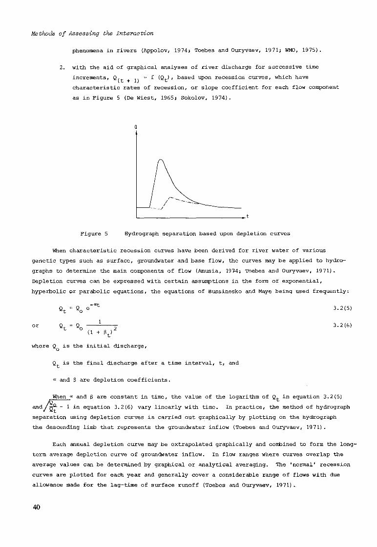
Methods of Assessing the Interaction
phenomena in rivers (Appolov, 1974; Toebes and Ouryvaev, 1971; WMO, 1975).
2. with the aid of graphical analyses of river discharge for successive time
increments, Q, = f (Q.), based upon recession curves, which have 11 + 1) t
characteristic rates of recession, or slope coefficient for each flow component
as in Figure 5 (De Wiest, 1965; Sokolov, 1974).
Figure 5 Hydrograph separation based upon depletion curves
When characteristic recession curves have been derived for river water of various
genetic types such as surface, groundwater and base flow, the curves may be applied to hydro-
graphs to determine the main components of flow (Amusia, 1974; Toebes and Ouryvaev, 1971).
Depletion curves can be expressed with certain assumptions in the form of exponential,
hyperbolic or parabolic equations, the equations of Bussinesko and Maye being used frequently:
*t o -Œt
ö t = Qo
(1 + 3t>"
3.2(5)
3.2(6)
where Q is the initial discharge,
Q is the final discharge after a time interval, t, and
œ and ¡3 are depletion coefficients.
v£ When <* and ß are constant in time, the value of the logarithm of p. in equation 3.2(5)
and/r^ - 1 in equation 3.2(6) vary linearly with time. In practice, the method of hydrograph
separation using depletion curves is carried out graphically by plotting on the hydrograph
the descending limb that represents the groundwater inflow (Toebes and Ouryvaev, 1971).
Each annual depletion curve may be extrapolated graphically and combined to form the long-
term average depletion curve of groundwater inflow. In flow ranges where curves overlap the
average values can be determined by graphical or analytical averaging. The 'normal' recession
curves are plotted for each year and generally cover a considerable range of flows with due
allowance made for the lag-time of surface runoff (Toebes and Ouryvaev, 1971).
40

Methods of Assessing the Interaction
To facilitate the extrapolation of recession curves one can use a semi-logarithmic scale,
the logarithmic one for discharge and linear one for time, which changes the depletion curve
into a straight line or a series of straight lines (De Wiest, 1965; Nutbrown and Downing,
1976).
During flood periods the depletion curve may be used to define the separation line and
estimate the period of maximum groundwater inflow. For this purpose the depletion curve is
extrapolated forwards in time at the start of the flood and back in time at the end of the
flood. The period of maximum groundwater inflow may be checked from regime data or from data
on the velocity of groundwater flow compared with that for river .flow. The chosen maximum
point is then connected by a straight line or smooth curve with the extrapolated depletion
curve.
In some cases it is necessary to estimate the separation line in a flood period by
extrapolating two depletion curves. The first has a relatively slow recession rate and is used
during the period when the total river flow is increasing, and the second is used to define
the groundwater recession after the period of maximum groundwater inflow as shown in Figure 6
(Riggs, 1953; Snyder, 1939). Use of the depletion curve analysis together with a water
balance equation for the river basin enables the flow separation to be completed in some
detail by analytical methods such as those described by Kalinin (1957).
Qn
2 5 •
za /
15 /
io A /
Figure 6 Determination of the depletion curve (1) and recessxon curve (2)
Improvements in the techniques of hydrograph separation using recession curves and
groundwater depletion curves must be based upon additional substantiating information,
including verification of the genetic classes of the flow components, conformity with the
hydrogeological basin characteristics as well as hydrometeorological and hydrogeological data.
3.3 Groundwater Table Fluctuations
Groundwater storage tends to fluctuate continuously in response to external factors in both
confined and unconfined aquifers. Corresponding fluctuations occur in the groundwater table
41

Methods of Assessing the Interaction
where variations in level may be either relatively rapid, such as seasonal, or long-term with
a duration of several years. The short-term variations may be caused by changes in atmospheric
pressure, earth tremors, precipitation or seepage from surface water. In addition human
interference such as the regulation of watercourses, drainage, and earth-works may cause short-
term or permanent and rapid changes in level.
This section is concerned with the variations in groundwater level caused by seasonal
changes in the hydrological cycle and with long-term changes caused by climatological
variations, mainly through their causal connection with surface water storage.
Groundwater storage changes occur because of differences between inflow rates to and
outflow rates from groundwater. This difference will vary in space and time, particularly from
one climatological zone to another due to different precipitation and evaporation patterns. In
some areas groundwater recharge may be derived predominantly from precipitation directly, and
in other areas from the infiltration of surface water. Groundwater level fluctuations in a
given locality tend to occur in a regular manner so that they may be used as an index of the
regime characteristics. Thus the groundwater regime may be classified by methods such as those
of Konoplyantsev and Kovalevsky (1963) which is based upon a water balance analysis and takes
-into account the interaction between surface water and groundwater. The main types of natural
groundwater regime of the USSR have been determined using this method. These main types of
regime are :
1. short-term recharge, mainly during the summer
2. seasonal recharge, mainly during the spring and autumn
3. annual recharge, mainly during the winter.
Divisions may be made within each of these three types to distinguish between the
various levels of recharge, whether of the abundant type of the temperate regions, scarce
type of the arid regions or hydrological types related to recharge from river flow. The
general characteristics of groundwater formation and its regime type depends upon various
natural factors. In the following sections the main features of groundwater level fluctuations
are described for two regions. Firstly for a temperate region (Nordic area) and secondly for
an arid region (northern Africa).
3.3.1 Temperate Areas
In temperate and humid environments where annual precipitation generally exceeds the annual
potential evaporation, groundwater is recharged mainly by precipitation. Groundwater flow in
these areas will tend to be towards rivers, where it becomes the base flow component of river
flow. Groundwater thereby combines with direct runoff to form the total river flow.
Where groundwater is recharged mainly from precipitation the changes in groundwater level
depend upon the characteristics and state of the unsaturated aquifer and overlying soil.
Important factors are the degree of saturation, effective porosity, permeability and the
42

Methods of Assessing the Interaction
distance that infiltrating water has to travel to reach the groundwater table. These factors
are responsible for a delay in the reaction of the groundwater table to rain. In the Nordic
countries the delay is usually small as the soil layer is generally rather thin and
predominantly Quaternary. This causes the groundwater table to follow closely the annual
rhythm of seasonal changes.
In the temperate areas of the Nordic countries the annual rhythm consists of three or
four distinct phases. The snow melt causes the groundwater table to rise with a maximum level
reached in March to May depending upon the locality. This is often the maximum for the year.
After this the groundwater table falls at a regular rate because of the effect of summer
evaporation. During the summer months evaporation is relatively high and there is a
negligible recharge of groundwater from precipitation. Groundwater recharge occurs again in
the autumn when rainfall exceeds evaporation and soils reach field capacity. Then in the
winter the surface of the soil becomes frostbound, infiltration more or less prevented and
the groundwater table again falls.
The effect of the soil frost in Nordic countries is to interrupt the hydrological cycle
for periods of two to seven months. This effect can be observed in groundwater hydrographs,
such as Figure 7 which shows the mean seasonal groundwater variation patterns for a number of
representative stations (Nordberg and Soveri, 19 78). The line showing mean groundwater levels
is based generally upon 10 to 26 years of record, and monthly mean precipitation and air
temperature is taken from adjacent official weather stations for the same period of observation.
There are four main groundwater regime patterns in the Nordic area. Denmark and southern
Sweden are in zone four, where the characteristic curves show a net recharge during the autumn
and winter months and declining groundwater levels for the remainder of the year. Proceeding
north from this area the increasing negative influence of the winter on recharge is apparent.
Over much of Sweden and Finland winter precipitation is in the form of snow, and since this
generally falls on frozen ground no groundwater recharge occurs in those months. This is also
true for much of Norway, but data from that country is at present insufficient to show the
different zones. Moreover, the steep topography and the influence of the Atlantic ocean pose
special problems that will have to be studied when more data becomes available. For these
reasons the lines on Figure 7 showing the boundaries of groundwater zones are not continued
into Norway.
Groundwater patterns in zone three indicate a secondary decrease in levels in the winter
which is observed mainly in a belt through south central Sweden. The characteristic patterns of
zone two show a more dominant influence of the winter, with the major recharge occurring in
connection with snow melt, and a minor recharge in the autumn before precipitation is in the
form of snow. Zone two occurs across north central Sweden, around the Gulf of Bothnia, in
southern Finland and in the adjacent parts of thé USSR. In zone one the characteristic pattern
indicates long winters with net groundwater recharge only during and immediately after snow
melt. This zone occupies the inland parts of northern Sweden, Finland and the USSR, with a
boundary some distance from the Baltic Sea (Nordberg and Soveri, 1978).
43

Methods of Assessing the Interaction
Figure 7 Mean seasonal groundwater variations in the Nordic countries and adjacent parts
of the USSR related to precipitation and air temperature
44
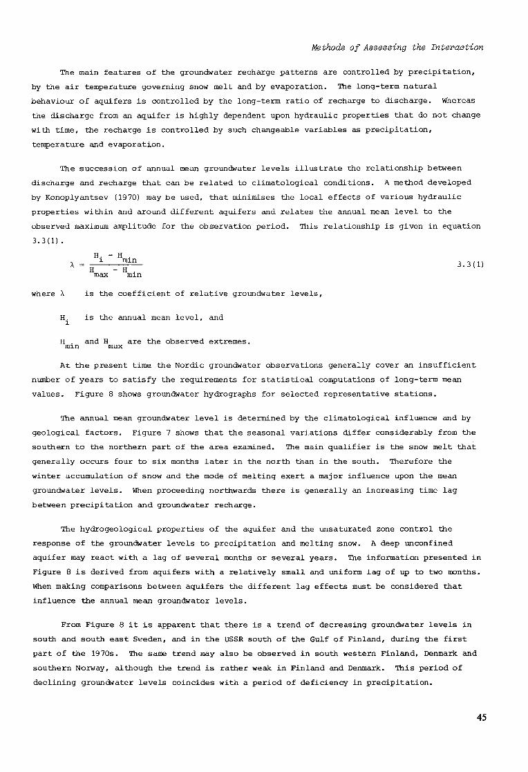
Methods of Assessing the Interaction
The main features of the groundwater recharge patterns are controlled by precipitation,
by the air temperature governing snow melt and by evaporation. The long-term natural
behaviour of aquifers is controlled by the long-term ratio of recharge to discharge. Whereas
the discharge from an aquifer is highly dependent upon hydraulic properties that do not change
with time, the recharge is controlled by such changeable variables as precipitation,
temperature and evaporation.
The succession of annual mean groundwater levels illustrate the relationship between
discharge and recharge that can be related to climatological conditions. A method developed
by Konoplyantsev (1970) may be used, that minimises the local effects of various hydraulic
properties within and around different aquifers and relates the annual mean level to the
observed maximum amplitude for the observation period. This relationship is given in equation
3.3(1) .
Hi ~ Hmin 3 < 3 ( 1 )
H - H . max m m
where X is the coefficient of relative groundwater levels,
H. is the annual mean level, and
H . and H are the observed extremes, mxn max
At the present time the Nordic groundwater observations generally cover an insufficient
number of years to satisfy the requirements for statistical computations of long-term mean
values. Figure 8 shows groundwater hydrographs for selected representative stations.
The annual mean groundwater level is determined by the climatological influence and by
geological factors. Figure 7 shows that the seasonal variations differ considerably from the
southern to the northern part of the area examined. The main qualifier is the snow melt that
generally occurs four to six months later in the north than in the south. Therefore the
winter accumulation of snow and the mode of melting exert a major influence upon the mean
groundwater levels. When proceeding northwards there is generally an increasing time lag
between precipitation and groundwater recharge.
The hydrogeological properties of the aquifer and the unsaturated zone control the
response of the groundwater levels to precipitation and melting snow. A deep unconfined
aquifer may react with a lag of several months or several years. The information presented in
Figure 8 is derived from aquifers with a relatively small and uniform lag of up to two months.
When making comparisons between aquifers the different lag effects must be considered that
influence the annual mean groundwater levels.
From Figure 8 it is apparent that there is a trend of decreasing groundwater levels in
south and south east Sweden, and in the USSR south of the Gulf of Finland, during the first
part of the 1970s. The same trend may also be observed in south western Finland, Denmark and
southern Norway, although the trend is rather weak in Finland and Denmark. This period of
declining groundwater levels coincides with a period of deficiency in precipitation.
45
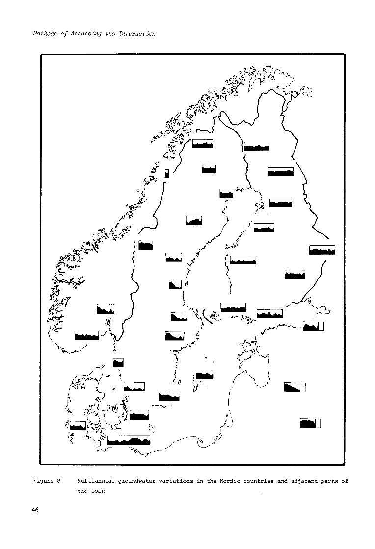
Methods of Assessing the Interaction
Figure 8 Multiannual groundwater variations in the Nordic countries and adjacent parts of
the USSR
46

Methods of Assessing the Interaction
The effects have been recorded in aquifers of many types, small and large, deep and shallow,
and confined and unconfined. In 1977 the decreasing trend was halted and some recovery took
place. Within areas of generally decreasing groundwater levels opposite trends have been
observed due to local conditions. In the remainder of the area shown in Figure 8 no clear
regional trends are detected. However several records from northern Sweden show increasing
levels during the 1970s (Nordberg and Soveri, 1978) .
The absolute change in groundwater level is qualified by the effective porosity and
permeability, and may vary from a few centimetres to several metres. This aspect is not
discussed in this report.
Periodicities in the multiannual variations have not been detected at a meaningful level
of significance possibly due in part to the rather short period of observation. Zaltsberg
(1977) reported periodicities of 4 to 5, 8 to 11, 16 to 17 and 25 to 27 years for groundwater
in western USSR and a periodicity of five years within an observation period of 11 years for
groundwater levels in Finland (Soveri, 1973). Rather longer periodicities were detected in
Lake Saima in Finland, and lake Vanern in Sweden (Nordberg and Soveri, 1978).
3.3.2 Arid Areas
In arid zones annual rainfall is always less than the potential evaporation. In most
instances there is not even a monthly water surplus. Because of the marked iregularity of i
rainfall a water surplus may be evident for just one day or a week during the wet period which
for example in Tunisia occurs from September to April. The response of the water table to this
discontinuous replenishment in the rainy season is a seasonal fluctuation in the piezometric
levels characterized by an annual minimum and maximum.
In parts of north Africa groundwater recharge occurs after the autumn rains, the water
table reaches the highest level in the spring and there is a recession throughout the summer.
When the water table is some depth below the soil surface infiltrating water may take some time
to pass through the unsaturated zone. Lowest levels often occur during September or October
and the highest levels in March or April. The volume of water involved in this seasonal
fluctuation of the water table defines the annual regulating capacity of an aquifer. Thus the
relationship between surface water and groundwater may be quantified by analysing the steady
state groundwater recession of the summer and the subsequent, water table recovery of the rainy
season.
In arid zones the direct infiltration of rainfall to groundwater does occur, but is
negligible compared with the inflow from rivers. Recharge from floods occurs mainly in the
piedmont zones. Consequently, in the case of an homogeneous aquifer, water table fluctuations
will generally be most apparent along the upstream part of an aquifer. This upstream zone
tends to be relatively permeable and it is in this region that the aquifer is periodically
recharged from surface flows during successive rainy seasons.
The rise of groundwater levels in the recharge zone after each flood is followed by a
gradual rise in the surrounding water table. The speed of this sideways movement of groundwater
47

Methods of Assessing the Interaction
depends upon the aquifer diffusivity and always occurs some time after the flood event. When
successive recharge events occur close together then recharge water from one flood will be
superimposed upon water from previous events, thus delaying the recession of groundwater levels
and adding to the groundwater storage. With increasing distance down gradient from the
recharge zone the fluctuations progressively decrease, until in the lower plains the effect of
floods is not easily measured. If there is no direct recharge by rainfall in the lower plains
then the effect of evaporation is to create almost steady state conditions with water table
fluctuations of less than one metre. In the recharge zone fluctuations may be several metres.
Where there are a sufficient number of piezometers and in cases where the aquifer is
approximately homogeneous it is possible to estimate the annual volume of recharge from surface
inflows. The areal extent of groundwater fluctuations of a given amplitude are plotted and
measured by planimetry to solve equation 3.3(2).
R = A. S. h 3.3(2)
where R is the volume of recharge
A is the area of groundwater fluctuation
S is the storativity or coefficient of storage, and
h is the mean amplitude of the fluctuations.
It is apparent that a lack of precision in determining the storativity (S) may
significantly reduce the accuracy of the estimated recharge. Indeed, this method demands a
considerable amount of field data. Also in the case of over-exploited aquifers it is necessary
to take into account the effect of pumping on the piezometer levels, because the demands of
water for agriculture are not related to the aquifer stage.
When the aquifer replenishment occurs mostly along one main river, the variations in
storage from a major replenishment event may be defined in a similar manner, but fewer
carefully sited piezometers are then necessary. In this case the volume of recharge water
during a rainy period may be estimated as follows:
1. identify for each piezometer and between two recession periods the aquifer
recovery after a flood (or successive floods),
2. draw similar recovery curves for the aquifer to determine the sections
saturated by flood water. This is achieved by plotting groundwater levels
along sections perpendicular to the river for successive time increments,
3. planimeter the recovery zones and estimate the specific yield.
This procedure ensures that the record of groundwater levels at each piezometer is
carefully analysed so that the flow increment corresponding to the rainy period is separated
analytically from the initial total flow of the aquifer when it was in a steady state
condition. To assist in the separation of the groundwater hydrograph it is necessary to know
48

Methods of Assessing the Interaction
the natural recession characteristics of the aquifer. With this information an estimate may be
made of the groundwater levels if aquifer recharge had not occurred. The general form of the
groundwater recession is similar to equation 3.2(6) and is:
qt = qo e"Πt 3.3(3)
where q is the groundwater flow at time t,
a is the groundwater flow when t = o, and
--f~»-£ -oct
In a laminar flow regime we also find that, h. = h e , where h and h represent the
hydraulic head related to the flow base level H. This base level is the asymptote towards
which h converges as t increases. To calculate the curve h (t) the first step is to estimate
H at any time during the steady state period, then the recession constant °= from the
experimental curve of groundwater level recession. The values of H and = depend upon the
position of the piezometer and on the diffusivity T/S at that point, and their determination
enables the characteristic recession curve to be drawn for the piezometer site. The recession
curves for all the other sites may be derived from a simple relationship based upon the delay
in groundwater recession. However, this method requires rather a precise knowledge of the
distribution of the specific yield for the whole area affected by the recovery of groundwater
levels. In addition, in zones far from the river relatively small variations in the water
table over large areas may be imprecisely estimated with a consequential decrease in the
accuracy of the inflow estimates. The main advantage of this method is its ability to
distinguish the contribution of each major flood to the aquifer replenishment.
Observations of groundwater level fluctuations over many years have shown that long
period variations exist which reveal the multiannual irregular characteristics of inflows.
There is a tendency for the random variation in rainfall to be stronger than the seasonal or
periodical variation with the result that seasonal variations in groundwater levels are not as
large as multiannular variations. The aquifers are able to store the inflows of successive
rainy years which slowly seep towards the lower plains and enter the next phase of the
hydrological cycle. Similarly, successive dry years may occur and result in a serious
depletion of groundwater flow. In parts of north Africa a ten year period has been observed
in the sequence of successive dry and wet years, and it is frequently observed that the
amplitudes of multiannual fluctuations are five times greater than the seasonal fluctuations.
The relationship between surface water and groundwater is difficult to evaluate in areas
with pronounced multiannual cycles because the variation of long cycles is more difficult to
characterise than short high frequency cycles. Long cycle variations may not be noticeable if
the period of observation is relatively short. Various integration techniques, such as the
'moving average' curve which smooth the amplitude of the series by filtering the high
fluctuations, may be used to analyse the variations of long inflow series as shown in Figure 9.
The relationship between inflows and the aquifer response may be examined by using moving
average techniques when these two variables are plotted with the same time scale.
49

Methods of Assessing the Interaction
800H
600 -
10
c ¡5
OC
(O 3 C C <
E 400 (0 0)
5
3 year moving average
rainfall
Groundwater Level
(in 0.1 m )
V. / Ma
i \ V \ /
h H \
I/ il
\ /
*y u ,•• "i
10 year moving average rainfall
V.
1920 1940 1960 Year
Figure 9 Groundwater levels and 3 and 10 year moving average rainfall in the Haut-Mornag,
Tunisia
Simple relationships may be derived between inflows (based upon rainfall or flood
discharge) and aquifer fluctuations using linear regression models with delayed effects. Long
series of data are frequently available for deriving such relationships which allow for the
effect of the aquifer inertia. These analyses include deriving a relationship (convolution
product) between the replenishment and a delay or transfer function which has assumed
parameters of length and shape. The transfer function is obtained from a knowledge of the input
series and output series (deconvolution). In some analyses an adjustment is made to the input,
flood inflows, and in estimates of the base level of the groundwater flow. However, these
techniques are essentially accurate only when applied to data from one piezometer and are
less useful for studying the phenomenon over larger areas. More complex models are suitable
for examining the relationship between surface water and groundwater in aquifer systems. These
include those based upon finite difference or finite element techniques.
3.4 Use of Isotopes as Tracers
3.4.1 Introduction
There are a number of problems associated with the interaction of surface water and groundwater
that may be solved conveniently by the use of a tracer, or built-in tracer, that reflects the
50

Methods of Assessing the Interaction
origin of the water. For example the question may arise as to whether pressure variations in
an aquifer indicate actual movement of water or a large range in values of aquifer permeability.
Tracers may be used to identify the mass transfer of water either from surface sources to
groundwater or in the reverse direction, and are useful in studies of water pollution.
The intentional injection of a tracer in groundwater is unlikely to give more than
relatively localised information on flow patterns except in cases of preferred flow paths in
fractured rock systems. However, the water molecules have built-in isotopic tracers that
reflect the origin of the water, and thus may be used to identify the occurrence and extent of
the movement of water between surface and groundwater systems. These natural tracers are the
stable isotopes deuterium and oxygen-18 and also the radioactive isotope of hydrogen known
as tritium, which although part of the water molecule, is not truly conservative because of its
radioactive decay. The term 'environmental isotope technique' in this context is defined as
the use of the variations in the environmental isotopic composition of natural waters as a tool
in hydrology. Other commonly used environmental isotopes in addition to the three already
mentioned include carbon-14 and carbon-13. The carbon isotopes are not actually part of the
water molecule but occur in water as dissolved inorganic carbon species.
This section summarises the causes which give rise to the variations in the environmental
isotopic composition of natural waters, the principles of their application to surface water-
groundwater interactions and examples of their use.
3.4.2 Stable Isotopic Composition of Natural Waters
The three main isotopic species of water, with their abundance in mean ocean water, are 16 16 18
H„ 0 (99.73%), HD 0 (0.031%) and H 0 (0.199%). The variations of the isotope ratios D/H •i O i /- ^
and 0/ 0 are measured in an isotope ratio mass spectrometer. The ratios are not measured
absolutely but are expressed in a S notation as a relative deviation from a standard.
6= ' ^ ' R s t d ' - 1 Q 3 3.4(1, Rstd
where R and R are the isotope ratios (D/H or 0 / 0) of the sample and standard
respectively.
The standard adopted is Vienna-SMOW (Standard Mean Ocean Water) which approximates to
the mean isotopic composition of the oceans. It will be noted that the delta values are
expressed in per mil. The usual analytical errors are 0.1%» and 1.0%« for oxygen-18 and
deuterium respectively.
When water changes phase, such as from vapour to liquid or vice versa, there is an
isotopic fractionation which results in a difference in stable isotopic composition of the
newly formed phase as compared to the other phase. The fractionation is greater the lower the
temperature. So in the condensation process for example there is a continual preferential
removal of the heavy isotopes deuterium and oxygen-18.
51

Methods of Assessing the Interaction
In practical terms this means that precipitation at higher latitudes is more depleted
than that at lower latitudes and winter precipitation is more depleted than slimmer
precipitation. Also, a very important property in applied hydrological studies, there is a
negative correlation of the heavy isotope content of precipitation with increase in altitude.
At any given season continental precipitation is more depleted in deuterium and oxygen-18 than
coastal precipitation. An overall global picture of the environmental isotopic composition of
precipitation is available from data obtained from the IAEA/WMO isotopes in precipitation
survey which commenced in 1961 (IAEA 1969; 1970; 1971; 1973; 1975; 1979). In the formation of
precipitation, deuterium and oxygen-18 behave in a similar way and the average global
correlation is:
ÔD = 8ô180 + 10 . 3.4(2)
Whereas the condensation process takes place in thermodynamic equilibrium this is not the
case for the evaporation process where the relationship given in equation 3.4(2) no longer
holds and the slope has a value in the range of about 4 to 6. Thus one finds that waters which
have been partially evaporated have a more enriched stable isotopic composition than their
feed water and fall below the meteoric water line defined by equation 3.4(2). In this way such
waters have a characteristic isotopic composition which may be used to study interactions
between lake water and groundwater.
3.4.3 Environmental Tritium Concentration of Natural Waters
Environmental tritium concentrations are normally expressed in TU (Tritium Units) where T —18
1 TU = — . 10 . Tritium (half life, 12.26 y) is produced by cosmic radiation in the upper H
atmosphere and also by the detonation of thermonuclear devices in the atmosphere.
Concentrations of tritium in precipitation resulting from cosmic ray production have been
estimated to be- about 10 to 20 TU depending upon geographic location. However, as a result of
the injection of tritium into'the atmosphere from thermonuclear devices, concentrations in
precipitation in the northern hemisphere were of the order of thousands of TU by 1963.
Concentrations in the southern hemisphere were very much less owing to the smaller number of
tests in that hemisphere and also the larger proportion of oceans to land mass. Since 1963
the concentrations have markedly decreased but in most parts of the world they are higher than
the estimated level of tritium due to the effect of cosmic rays.
Once precipitation with a given concentration of tritium has infiltrated into the ground
the tritium gradually decays and for all practical purposes no detectable tritium is present
after about 40 or 50 years. Surface waters forming from runoff from precipitation always
contain tritium. However, during prolonged dry periods when the proportion of groundwater in
river flow is high, quite low tritium concentrations may be observed. Because of the facts
outlined above it will be appreciated that the use of environmental tritium by itself is of
limited use for investigating the relationship between surface water and groundwater. However,
it may be useful when interpreting stable isotope data as a qualitative indication of the time
since recharge.
52

Methods of Assessing the Interaetion
3.4.4 Recharge of Groundwater by Rivers
The solution of a problem by isotope analysis in cases where groundwater is recharged by a
river is based upon the fact that a river contains water which has been derived from
precipitation falling on ground at higher altitudes than the area where river-groundwater
interactions are being studied. As a result of the effect of altitude the stable isotopic
composition of the river water will be more depleted than that of the groundwater if this has
been derived from the infiltration of precipitation falling directly on the area under
investigation. Therefore the stable isotopic composition of groundwater is compared with the
stable isotope indices estimated for the two potential sources of recharge.
The magnitude of the altitude effect for oxygen-18 is about -0.2 to -0.3%° per 100 m
change in elevation, that is two to three times the measurement accuracy. Normally a river
will contain water which has been derived from precipitation that has fallen at different
altitudes in the basin up to the maximum of the watershed. By the time the river has reached
the study area it will have integrated all the inputs from different elevations and the final
stable isotope index of the river water will reflect the oxygen-18 contents at different
elevations weighted by their respective volumetric inflows. Therefore it may be difficult to
estimate the stable isotope index purely from the topography of the basin.
A study in Ecuador illustrates the use of the isotopes as tracers (Payne and Schroeter,
1979) . The project area is about 20 km east of Guayaquil extending from Bucay, where the
River Chimbo leaves the Andes mountains, to Yaguachi in the western extremity. Shallow
groundwater was sampled at the end of the dry season from 51 open and closed wells fitted with
handpumps in a deltaic fan of sedimentary deposits in which the groundwater is about 3 m below
the ground surface (Figure 10). The variation in the stable isotopic composition of the
shallow groundwater extended over a range of 4%o and 30%o for oxygen-18 and deuterium
respectively (Figure 11). This indicated that the shallow groundwater is a mixture derived in
varying proportions from two sources each having its own characteristic stable isotopic
composition.
Figure 12 shows a histogram of the frequency distribution of the SD values of the shallow
groundwater excluding two samples which exhibit a marked effect due to evaporation. The
distribution is highly skewed with the maximum frequency close to the stable isotopic index
estimated for recharge by the infiltration of local precipitation. The lower frequency occurs
at delta (i.e. 6) values close to that of the river water. The latter being estimated from
actual river samples and groundwater which was clearly recharged by the river. Analyses of
water from individual wells indicated the proportions and areal extent of the river water
recharge to the shallow groundwater.
Morgante et al (1966) studied the infiltration of water from the Isonzo river to ground-18
water in the Gorizia plain in north eastern Italy. The 6 0 values of groundwater from 32 wells
were measured at various times between December 1963 and April 1965, and the Isonzo river water 18
was sampled between March 1964 and April 1965 at different locations. The mean 6 0 value was 18
close to -10%». It was apparent that the 6 0 values for groundwater became more positive with
53

Methods of Assessing the Intevaotion
•-25.7 • -24.1
O - 2 7 7
• -24.5 •-22.1
-29.10 9 # . 2 9 1 # . 2 5 1
-26.3 # . 3 A 8
\ * - 2 9 . 2
o OPEN WELLS
# . 2 7 5 • HAND-PUMPED WELLS
X Y A G U A C H I _^2 # -23 .6
Ly_ -46.8 • -29 9 T V MILAGRO0 -2°4 • "g3
#VVs/^~^2/ l7J -25.3 -258 ^
" 4 A 8 ^ ^ é - 2 6 2 . 0 0 - 2 7 ° O - ^ -23.5»^N^.557 • 0 . 2 7 1 SAN -2A.8. \ 3 7 ¿ ^ 6 o 2 4 6 C A R L O S
-23°2 . -261 ̂ i ¿ ß ^ ^ -23.6 Ä ^
•-29.5
N
\
• -28.1
• -29.6
• -30 0-24.9
• -29.3
^ r^T-^O CHIMBO BUCAy
_ - 4 0 . 9 • ••36.4 g —
RIO CHANCHAN ^ T • -276 V
• -43.8 N.
0 5 10Km -•vi ^ ^ 1
•
Figure 10 Deuterium content of shallow groundwater bordering the Rio Chimbo in Ecuador
-10T
-6 -5 -4
OXYGEN-18 %o
Figure 11 Stable isotopic composition of shallow groundwater
54
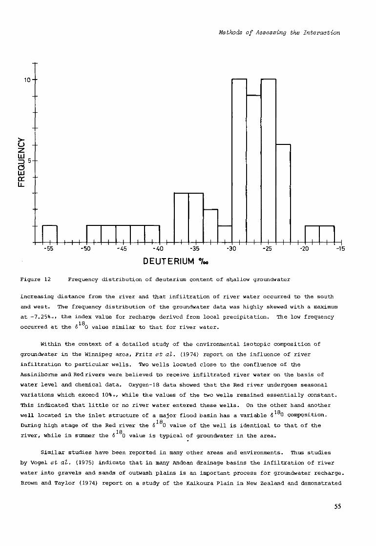
Methods of Assessing the Interaction
10--
>-O -f w R
a5
o LU er ü.
H—H- + 15 -55 -50 -45 -40 -35
DEUTERIUM %o -30 -25 -20
Figure 12 Frequency distribution of deuterium content of shallow groundwater
increasing distance from the river and that infiltration of river water occurred to the south
and west. The frequency distribution of the groundwater data was highly skewed with a maximum
at -7.25%o, the index value for recharge derived from local precipitation. The low frequency In
occurred at the 5 0 value similar to that for river water.
Within the context of a detailed study of the environmental isotopic composition of
groundwater in the Winnipeg area, Fritz et al. (19 74) report on the influence of river
infiltration to particular wells. Two wells located close to the confluence of the
Assiniborne and Red rivers were believed to receive infiltrated river water on the basis of
water level and chemical data. Oxygen-18 data showed that the Red river undergoes seasonal
variations which exceed 10%», while the values of the two wells remained essentially constant.
This indicated that little or no river water entered these wells. On the other hand another 18 well located in the inlet structure of a major flood basin has a variable 6 0 composition.
18 During high stage of the Red river the 6 0 value of the well is identical to that of the
18 river, while in summer the 6 0 value is typical of groundwater in the area.
Similar studies have been reported in many other areas and environments. Thus studies
by Vogel et al. (1975) indicate that in many Andean drainage basins the infiltration of river
water into gravels and sands of outwash plains is an important process for groundwater recharge.
Brown and Taylor (1974) report on a study of the Kaikoura Plain in New Zealand and demonstrated
55

Methods of Assessing the Interaction
the importance of recharge by infiltrations from the Kowhai river. The technique is also
proving valuable in arid zones for assessing recharge by flash floods in wadis.
An increasing number of municipal water supplies are indirectly or directly linked to
rivers. In many instances an improvement in water quality is possible if river water
infiltration is induced and the water pumped once it has passed through river gravels and sand.
However, if the wells are too far removed from the river they draw on both river water and
local groundwater. In a study of the water supply system of the city of Bern, Siegenthaler
and Schotterer (1977) demonstrated the increase of the groundwater component with increasing
distance from the Aare river.
To accurately estimate the proportion of river water in groundwater depends upon the
accuracy of the estimates of the stable isotopic indices of the two potential sources of
recharge and the difference between these indices. An estimate of the river index may be made
on the basis of samples taken from the river. This should be done at different times and river
stage to ascertain whether there are any significant variations in the stable isotopic
composition. If variations are evident then the mean value weighted for discharge should be
used. A quicker and preferable approach is to sample groundwater close to the river where
groundwater levels indicate that river water is the source of recharge. The estimation of the
index for recharge by infiltration of local precipitation may be based on measurements of
groundwater away from the influence of the river or, if sufficient data are available, on the
peak value of the skewed frequency distribution. If the errors in the estimates of the indices
of the two potential sources of recharge are not greater than the analytical error, then the
accuracy in the estimate of the proportion is better than 10%.
An example of the use of tritium and carbon-14 is provided by a study to assess the
environmental impact of the construction of a nuclear plant in the upper reaches of the Reno
river (Carlin et al., 1975).. The investigation assessed the relationship between the Reno
river water and groundwater in the area of Bologna. At two pumping stations the tritium and
carbon-14 content of the groundwater decreased with increasing distance from the river. This
demonstrated the contribution of river water to the aquifer. At a distance of about 700 m
from the river the effect of this contribution by the river was found to be negligible. At
another pumping station which was commissioned more recently and is located further from the
river, no influence of river water was detected. However, it is conceivable that as a result
of prolonged pumping water derived from the river may ultimately also reach this station. By
monitoring the tritium and carbon-14 content this possibility would be checked.
Conclusions concerning the origin of recharge water are based on the analyses of ground
water samples. This implies the availability of sampling points tapping specific horizons
that are sufficient in number and spatial distribution to provide a representative coverage of
the area under investigation. In practice the limitations of the method are not caused by the
method itself, but by the availability of meaningful samples.
56

Methods of Assessing the Interaction
3.4.5 Recharge of Groundwater by Lakes
The interaction between lake water and groundwater may be examined by isotope analysis
provided that the stable isotopic composition of the lake is significantly different from that
of recharge derived from local precipitation. Lake water undergoing partial evaporation is
enriched in deuterium and oxygen-18 along evaporation lines with a slope of four to six and
may therefore be differentiated from samples falling on the meteoric water line of slope 8.
In some cases the evaporation effect on the lake water may be minimal, but if the inflow to
the lake is derived from higher elevations then the problem may be treated in the same manner
as for river-groundwater interactions.
18 As early as 1962 Gonfiantini et al. published 6 0 data on groundwater in the region of
In Lake Bracciano in Italy. The average ô 0 of groundwater was -6.0%» while that of the lake
was 0.69%o which demonstrated the independence of the two systems. The samples covered the
period June 1960 to March 1961 and little or no variability outside analytical error was
evident.
Lake Chala is a volcanic crater lake located at 840 m on the SE slope of Mount
Kilimanjaro on the border between Kenya and Tanzania. The lake has neither surface inflow nor
outflow and in connection with the possible expansion of a nearby irrigation scheme the problem
was to know the relationship between the lake water and springs in the area (Payne, 1970).
Samples of groundwater were analysed for their stable isotopic composition from ten locations,
at different depths and on two occasions nine months apart. No significant variation greater
than the analytical error was found. Samples of spring water were analysed also and in most
cases over a period of three years.
Figure 13 shows that the stable isotopic composition of the lake is markedly different
from that of the groundwater samples which fall on the meteoric water line. It was therefore
concluded that none of the springs studied received any significant contribution of water from
Lake Chala. Taking into account measurement errors the maximum possible cpntribution to
individual springs would not be more than a few per cent of their respective discharges.
Fontes et al. (1970) studied the influence of water from Lake Chad on the groundwater
system in the neighbourhood of the lake. The groundwater close to the north east side of the
lake has a stable isotopic composition which is indicative of an appreciable contribution of
lake water but only over a relatively short distance from the lake. Further away from the lake
the groundwater becomes more depleted in stable isotopic composition which reflects the
increasing proportion of recharge from rainfall that infiltrates into the dunes during the
summer rainy season.
A quantitative assessment of the relationship between lake water and a groundwater system
is not possible with a small number of samples if there is some variability in the composition
of the lake and groundwater. In fact it is the seasonal variation of the isotopic composition
of lake water which is a limiting factor in the sensitivity of the method.
57

Methods of Assessing the Interaction
20.0T Ó D % O
LAKE CHALA
D Ô180%o
30.0-1-
Figure 13 Stable isotopic composition of Lake Chala and groundwater in the area
3.4.6 Groundwater to Surface Water
The tritium concentration in the river Thet, United Kingdom, was measured and compared with
the concentrations in rainfall and groundwater (section 5.1, Case Study 1). Analyses of
samples showed a seasonal trend in the tritium concentration for both rainfall and river flow.
Equation 3.4(3) is typical of those derived based upon 31 samples taken in 1968.
T = 41 + 0.7 T F d 3.4(3)
where T is the tritium concentration in river water, in TU
T is the tritium concentration in rainfall, in TU r '
F is the proportion of direct runoff in river flow.
Although this equation accounts for less than 70 per cent of the total variance in T, it
quantifies an important factor, that the tritium concentration in river water tends to increase
as the proportion of direct runoff increases. This is because the concentration in rainfall
tended to be relatively high, between 70 and 250 TUs in the example given, and the
concentration in groundwater is typically just above zero. In addition summer rainfall tended
to have a higher tritium concentration than winter rainfall with lower values frequently
associated with the more intense rainfall events. Thus there is a tendency for concentrations
in major flood flows to decrease.
In the summer months the tritium concentration in river flow is typically low in spite of
the fact that the value for rainfall is high. This can be explained by hydrograph separation
exercises which indicate that summer flows generally have a high groundwater component with a
58

Methods of Assessing the Interaction
low tritium concentration, and only a small proportion of summer rainfall reaches watercourses
due to the effect of evaporation.
3.5 Use of Mathematical Models
3.5.1 Purpose of Modelling
Quantitative assessments of the interaction between surface water and groundwater should be
based on mathematical modelling. In recent years computers have become increasingly available
to solve complex or tedious mathematical problems, and this development has increased the
understanding of the interaction process. Models of the interaction should be based on
conceptual models of the hydrological cycle, for specific conditions of the water body under
study and may include for example a coupled surface and groundwater model (Cunningham and
Sinclair, 1979). In particular an adequate account should be taken of the mechanisms that
lead to the formation of surface water and groundwater.
One of the main purposes of modelling the interaction process is to investigate whether
assumed parameters and mechanisms are realistic. Thus, for example, if the assumed interaction
between a river and an aquifer is incorrect, then this will result in an inadequate model
response in terms of groundwater heads or flows when comparisons are made with field data. In
such cases it may be possible to use the model to investigate the type of mechanism that should
be introduced. A frequent problem encountered in practice is insufficient reliable field data
and a simplified mathematical model may then be used.
Another purpose in modelling is to investigate the effects of human interference in the
surface water or groundwater regime such as the effect of groundwater abstraction, river
regulation and changes in water quality. Water quality models are not discussed in detail in
this report since they are covered by other IHP Working Groups such as 6.3 and 8.1.
When considering the effect of the groundwater level, it should be noted that it has
little influence upon the recharge mechanism except for shallow aquifers. In contrast the
groundwater level is of critical importance in the interaction between aquifers and springs,
rivers, canals and lakes. When water flows to or from an aquifer the quantity flowing is very
sensitive to the difference in head between the surface source and the aquifer, differences
of one metre having a very significant effect. A head difference of one metre is small
compared with a head difference of say 100 metres which may occur in some areas. This must be
seen in the context of modelling the groundwater head when the accuracy is usually no better
than three per cent or approximately three metres.
Another important feature is that springs, rivers or canals are small in dimension
compared with the overall aquifer. Thus a spring, river or canal is in effect a mathematical
singularity. The flow patterns are complex in the regions of the interaction between surface
water and groundwater because of the small size of the region of the interaction compared with
the overall size of the drainage basin or aquifer. Therefore it is advisable to use a
detailed model of the aquifer. Proven techniques are available for modelling regional
groundwater flow using finite difference or finite element methods (Prickett, 1975). There is
59

Methods of Assessing the Interaction
no basic difference in the methods and therefore, for simplicity of presentation, reference
will be made initially to the finite difference technique followed by an example based upon
finite elements.
3.5.2 Groundwater Recharge
There are many alternative methods of evaluating recharge to an aquifer. Some are based on a
soil moisture balance (Penman, 1949) whilst others consider the flow in the unsaturated zone
(Van Keulen, 1975). However the interaction between surface water and groundwater in the
outcrop area is often more complex than the above models suggest and they tend to underestimate
the quantity of water entering the aquifer due to precipitation. For example, the soil
moisture balance method of Penman assumes that recharge occurs only when the soil is at field
capacity, i.e. when there is no soil moisture deficit. Consequently it is estimated that in
temperate climates there is negligible aquifer recharge during the summer months. However,
observation well data indicates that recharge does occur sometimes during the summer as shown
by a partial recovery in the groundwater head. Furthermore, the quantity of recharge as
calculated by the above method often leads to excessive declines in the groundwater head when
incorporated in a mathematical model. Alternatively this may be due in part to errors in
evaporation estimates (Anon, 19 78).
A careful field investigation of outcrop areas indicates that a proportion of the
precipitation can enter an aquifer by-passing the soil zone. Sometimes this occurs when the
runoff from steeply sloping ground enters the aquifer via natural 'swallow' holes (Fox and
Rushton, 1976). In other situations natural drains lead directly into an aquifer. Though
field responses indicate that some water does enter certain aquifers by-passing the soil
moisture, it is essential to check such an assumed mechanism by incorporating it in a
mathematical model of the aquifer. Only then is it possible to check whether the correct
response occurs in the observation wells. Also the general trends in aquifer heads and flows
indicate whether the total recharge is of the correct order of magnitude (Spink and Rushton,
1979).
The depth of the water table below the soil zone can vary from a fraction of a metre to
hundreds of metres. Unless this distance is small, the passage through the unsaturated zone
can be important, particularly due to the effect of increasing nitrates in groundwater. Model
studies have shown that in some aquifers the flow mechanisms in the unsaturated zone are such
that the downward movement of water through the fissure system has a typical vertical flow rate
of 0.7 m/day whereas the vertical flow rate of the solutes is only 1 m/year (Oakes, 1977). In
this study the flow rate was estimated by an equation relating the response of the water table
to estimated infiltration at the surface. Approximately 15 per cent of the infiltration
reached the water table during the first month and the remainder in succeeding months. The
time taken for infiltration to flow through the unsaturated zone depends upon the distance
from the ground surface to the water table and the properties of the aquifer. In his
discussion on the rate of solute transport, Oakes considered the movement of both tritium and
nitrate profiles. If it is assumed that solutes diffuse from the infiltrating water into the
relatively static water in the rock matrix then this can account for the slow downward
60
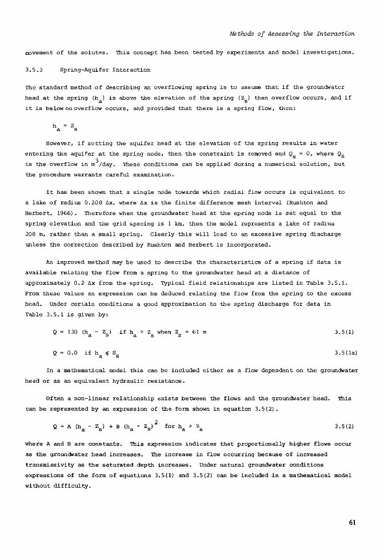
Methods of Assessing the Interaction
movement of the solutes. This concept has been tested by experiments and model investigations.
3.5.3 Spring-Aquifer Interaction
The standard method of describing an overflowing spring is to assume that if the groundwater
head at the spring (h ) is above the elevation of the spring (Z ) then overflow occurs, and if a s
it is below no overflow occurs, and provided that there is a spring flow, then:
h = Z a s
However, if setting the aquifer head at the elevation of the spring results in water
entering the aquifer at the spring node, then the constraint is removed and Q = 0 , where Qs
3 is the overflow in m /day. These conditions can be applied during a numerical solution, but the procedure warrants careful examination.
It has been shown that a single node towards which radial flow occurs is equivalent to
a lake of radius 0.208 Ax, where Ax is the finite difference mesh interval (Rushton and
Herbert, 1966). Therefore when the groundwater head at the spring node is set equal to the
spring elevation and the grid spacing is 1 km, then the model represents a lake of radius
208 m, rather than a small spring. Clearly this will lead to an excessive spring discharge
unless the correction described by Rushton and Herbert is incorporated.
An improved method may be used to describe the characteristics of a spring if data is
available relating the flow from a spring to the groundwater head at a distance of
approximately 0.2 Ax from the spring. Typical field relationships are listed in Table 3.5.1.
From these values an expression can be deduced relating the flow from the spring to the excess
head. Under certain conditions a good approximation to the spring discharge for data in
Table 3.5.1 is given by:
Q = 130 (h - Z ) if h > Z when Z = 61 m 3.5(1) cL S 3. S S
Q = 0.0 if h « S 3.5(la) a s
In a mathematical model this can be included either as a flow dependent on the groundwater
head or as an equivalent hydraulic resistance.
Often a non-linear relationship exists between the flows and the groundwater head. This
can be represented by an expression of the form shown in equation 3.5(2).
Q = A (h - Z ) + B (h - Z ) for h > Z 3.5(2) a & d o cl a
where A and B are constants. This expression indicates that proportionally higher flows occur
as the groundwater head increases. The increase in flow occurring because of increased
transmissivity as the saturated depth increases. Under natural groundwater conditions
expressions of the form of equations 3.5(1) and 3.5(2) can be included in a mathematical model
without difficulty.
61
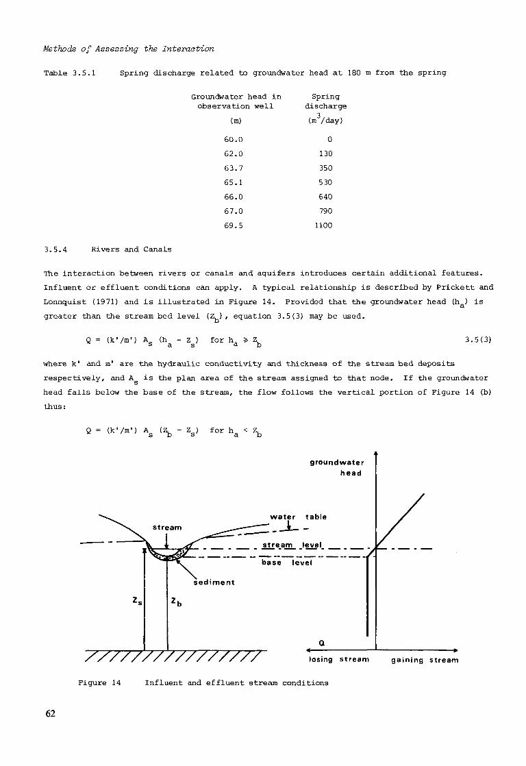
Methods of Assessing the Interaction
Table 3.5.1 Spring discharge related to groundwater head at 180 m from the spring
Groundwater head in observation
(m)
60.0
62.0
63.7
65.1
66.0
67.0
69.5
well Spring
discharge 3
(m /day)
0
130
350
530
640
790
1100
3.5.4 Rivers and Canals
The interaction between rivers or canals and aquifers introduces certain additional features.
Influent or effluent conditions can apply. A typical relationship is described by Prickett and
Lonnquist (1971) and is illustrated in Figure 14. Provided that the groundwater head (h ) is
greater than the stream bed level (ZL ) , equation 3.5(3) may be used.
Q = (k'/m') A (h - Z ) for h » Z^ 3.5(3) s a s a b
where k' and m' are the hydraulic conductivity and thickness of the stream bed deposits
respectively, and A is the plan area of the stream assigned to that node. If the groundwater
head falls below the base of the stream, the flow follows the vertical portion of Figure 14 (b)
thus:
Q = (k'/m1) As (Zb - Zg) for h & < Z^
groundwater head
water table
stream level
base level
sediment
/ / / / / / / / / / / / / / / / losing stream gaining stream
Figure 14 Influent and effluent stream conditions
62

Methods of Assessing the Intevaat-ion
There are a number of difficulties associated with equation 3.5(4). The first is that it
is difficult to ascertain the values of the parameters k' and m'. Equally important is the
difficulty of defining what is meant by the groundwater head at the stream h - An examination a
of the form of the flow pattern in the vicinity of a partially penetrating stream demonstrates
that significant changes in head may occur. In particular the groundwater head may vary
significantly on the vertical below the stream. Certain attempts have been made to allow for
the complex flow patterns near to a stream. Aravin and Numerov (1953) make allowances for this
effect by means of equivalent seepage resistances which are determined from analytical
solutions which represent the curvature of the streamline. Another approximation by Herbert
(1970) leads to similar results. These expressions for the additional resistance to flow can
be written in a form similar to equation 3.5(3) and can be included without difficulty in a
numerical model. In practice a non-linear relationship is often more appropriate with the flow
described by an expression of the form of equation 3.5(5) (Rushton and Tomlinson, 1979).
1 - exp { - D (h - Z ) } a. Ö
3.5(5)
where C and D are constants.
Although it is difficult to ascertain suitable values for the properties of the stream
bed, they do have a significant effect on the interaction between an aquifer and river or 3,
canal. For example when the inflow per unit length of a river is 0.225 m /day, a range of
head differences may be assumed to cause this leakage as shown in Table 3.5.2. The increase
in base flow in a specific reach is equivalent to the total leakage in that reach which may
be defined in terms of a leakage coefficient.
Table 3.5.2 Head differences related to leakage coefficient
Leakage Coefficient Head difference
(m) (m/day)
( k ' / m 1 ) A per unit length
0 .01 2 2 . 5
0.2 1.125
2 0.1125
5 0.045
The conditions with a head difference of 0.01 m approximate to those of a fully
penetrating river. Each of these values was used in turn in a finite difference model to
represent the flow to a river over a period of several years, and the results are shown in
Figure 15.
Using the four leakage coefficients relatively large and significant variations in
aquifer head are shown to occur compared with the small variations in the inflow along an 8 km
length of river. Indeed, when the recession part of the curve is examined in detail (Figure
16), the differences in flow are negligible for a relatively large variation in the leakage
coefficient. This result is particularly important because it indicates that an adequate
63

Methods of Assessing the Intevaction
85
80
•o 75 ra u
X
70
65
Leakage Coefficients
K ( m / d )
0 . 0 4 5
0 . 1 1 2 5
1.125
22.5
Year
Flow proportional to
head difference
v o> (D JÉ at
Year
Figure 15 Four year cycle of groundwater inflow to a river with variable head differences
and leakage coefficients
agreement between modelled and measured base flow during a recession period does not
necessarily mean that a satisfactory model of the river has been obtained. Also it indicates
why a model may appear to be satisfactory when a partially penetrating river has been assumed
to be fully penetrating if comparisons are made only between modelled and measured base flow.
64

Methods of Assessing the Interaction
In these circumstances the model could provide a poor representation of groundwater heads at
some distance from the river during recharge periods.
Leakage Coefficients
K( m/d)
*
o
Year 2
Figure 16 Annual cycle of groundwater inflow to a river with variable leakage coefficient
3.5.5 Lake-Aquifer Interaction
The interaction between a lake and an aquifer is different to that of a spring, river or canal
because the area of contact between the lake and the aquifer is much larger. Consequently
the flow patterns in the vicinity of the lake tend to be more complex, so that water may flow
from the aquifer into the lake in one region whereas in another region the same lake water may
be transmitted from the lake back into the aquifer. Two other features that often have a
dominant effect on the interaction are the hydraulic conductivity of the sediments at the
bottom of the lake and the ratio between the horizontal and vertical hydraulic conductivity
of the underlying aquifer.
Typical examples of the complexity of the flow patterns are given by Winter (1976). He
examines a number of single and multiple lake systems by the use of a mathematical model
65
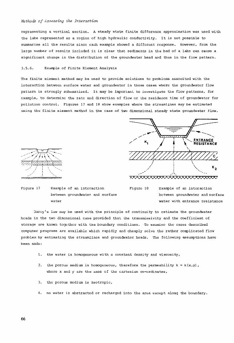
Methods of Assessing the Interaction
representing a vertical section. A steady state finite difference approximation was used with
the lake represented as a region of high hydraulic conductivity. It is not possible to
summarise all the results since each example showed a different response. However, from the
large number of results included it is clear that sediments in the bed of a lake can cause a
significant change in the distribution of the groundwater head and thus in the flow pattern.
3.5.6. Example of Finite Element Analysis
The finite element method may be used to provide solutions to problems associted with the
interaction between surface water and groundwater in those cases where the groundwater flow
pattern is strongly schematised. It may be important to investigate the flow patterns, for
example, to determine the rate and direction of flow or the residence time of groundwater for
pollution control. Figures 17 and 18 show examples where the streamlines may be estimated
using the finite element method in the case of two dimensional steady state groundwater flow.
V////^/}//)(/////^VA
9^y^TF7^^7^7^7^^l^5^5Si5i5l5'??^7 yJVWWWWJs^^
Figure 17 Example of an interaction
between groundwater and surface
water
Figure 18 Example of an interaction
between groundwater and surface
water with entrance resistance
Darcy's law may be used with the principle of continuity to estimate the groundwater
heads in the two dimensional case provided that the transmissivity and the coefficient of
storage are known together with the boundary conditions. To examine the cases described
computer programs are available which rapidly and cheaply solve the rather complicated flow
problem by estimating the streamlines and groundwater heads. The following assumptions have
been made :
1. the water is homogeneous with a constant density and viscosity,
2. the porous medium is homogeneous, therefore the permeability k = k(x,y),
where x and y are the axes of the cartesian co-ordinates,
3. the porous medium is isotropic,
4 . no water is abstracted or recharged into the area except along the boundary.
66

Methods of Assessing the Interaction
The area being examined is divided into elements and with the aid of computer programs
the potentials are calculated (case A). Using these potentials and the estimated inflow and
outflow along the boundary another groundwater flow problem is created (case B), such that the
calculated potentials for case B are the streamlines for case A.
The porous medium may be non-homogeneous with a discontinuity in the transmissivity as
shown in Figure 19. Values of the transmissivity used in case B now have to be determined.
Perpendicular to the plane of division the flow towards and from the plane is equal, so with
the notation in Figure 19:
Vnl = V n2
hence
dh dh
k l . — .cos91 = k2 . — 1
cos 6,
also
b = dl. dl„
sin 6,
or dl sin 6 = dl sin 9
Between two equipotential lines
dhL = dh2
hence kl t g 91 k2 * 62
3.5(6)
Figure 19 Porous medium with a discontinuity
To calculate the streamlines for case A there is the necessity of first determining the
equipotential lines of case B. If the equipotential lines in case A are perpendicular to the
equipotential lines of case B then:
67

Methods of Assessing the Interaction
tg 91 . tg V1 = -1
tg 92 . tgï2= -1
where f. and ¥ are the angles with the normal in case B.
3.5(8) it follows that:
k 2 ^ \
which means that to solve the flow problem, case B, the reciprocal values have to be used to
those for flow problem A.
As an illustration of the technique a schematical cross section has been drawn of two
aquifers and a drainage ditch with various assumed hydrogeological parameters (Figure 20).
The section has an impermeable base at a depth of 25 metres below the phreatic surface and the
vertical line below the centre of the ditch can be considered as representing an impermeable
boundary in the flow problem assuming that conditions are symmetrical about this line. At an
horizontal distance of 50 metres from the centre of the ditch, fixed head conditions are
assumed to exist in both aquifers with the head at that point being constant at 1 m above that
of the ditch. The input to the upper aquifer from effective rainfall is assumed to be 1 mm/day.
Separating the two aquifers is a semi-permeable layer with a resistance of 10 days and a thick
ness of 2 metres. On either side of this semi-permeable layer the aquifers have a permeability
of 5.1 m/day over a thickness of 2 metres, and the remainder of the aquifers have a
permeability of 10 m/day.
The ditch illustrated in Figure 20 is assumed to have a bed and sides with relatively
low permeability resulting in an entrance resistance of 1 day. Surrounding this area of low
permeability is an additional, layer with a thickness of 1 metre and a permeability of 5 m/day.
From this information the groundwater head may be estimated in each part of the cross section
using the finite element technique. For the solution of this problem the program 'STRATRECT2'
was applied which is available at the National Institute of Watersupply in the Hague. This
program uses rectangular elements of various sizes to schematise the reality. To solve the
problem outlined above the flow region was divided into 272 nodes and 240 elements. The output
gave the groundwater head at every nodal point and outflow or inflow of water along the
boundary.
The distribution of the heads is shown in Figure 21. From a knowledge of the estimated
inflows and outflows along the boundary the stream function along the boundary can be
calculated. Thus as described previously this stream function may now be used to define a new
groundwater flow problem (case B). Again the program 'STRATRECT2' is used to calculate the
heads with the results as illustrated in Figure 22. These equipotential lines are now the
streamlines for the first groundwater flow problem.
The advantage of this method is that the value of the stream function is calculated at
all the nodal points in the flow region. This means that the direction and volume of water
3.5(7)
3.5(8)
From equations 3.5(6), 3.5(7) and
68

Methods of Assessing the Interaction
Figure 20 Cross section with given hydrogeological parameters
flowing in any part of the section may be determined readily in addition to the residence
times which are important for example in problems associated with water quality. Thus the
characteristics of the interaction between groundwater and surface water can be determined by
varying the soil parameters such as the entrance resistances of ditches, the resistance of
clay layers and the permeability of the porous media.
3.5.7 Rainfall-Runoff Models
Many types of mathematical model have been developed for estimating river flows from weather
information (Clarke, 1975). Some contain conceptual representations of the hydrological cycle
including the inflow of groundwater to a river or the flow of river water to an aquifer. Other
models contain both conceptual and regression components.
The relationship between geology and streamflow characteristics has been studied for many
years with particular attention given to examining the areal variability of low flows
(Schneider, 1965} Vladimirov, 1966). Recent studies have included the ranking of rook types
according to their ability to maintain low flows and determining the relationship between
various low flow measures and basin characteristics. Thus an estimation of the flow duration
curve, flow frequency curve and storage-yield relationships for ungauged basins have been found
69

Methods of Assessing the Interaction
Figure 21 Equipotential lines for case A
Figure 22 Equipotential lines for case B which are identical to the flow lines for case A
70

Methods of Assessing the Interaction
to depend mainly upon an assessment of the properties of the underlying geology (UK, Inst, of
Hydrology, 1980). In addition certain geological formations and soil types have been shown to
have a major influence upon the magnitude of the mean annual flood (UK, NERC, 1975).
Various types of geological index have been used to quantify the influence of geology
on river flows. One form of this index is based upon the variability of daily, monthly or
seasonal low river flows. Another is the Base Flow Index that has been derived from the
recession characteristics of rivers (UK, Inst, of Hydrology, 1980). In this report the
results are presented for a monthly model that has been used to relate river flows to rainfall
less evaporation in over 70 representative basins in England and Wales (Wright, 1978). The
equations that were derived for each river have been examined to quantify certain aspects of
the influence of geology on river flows. Two examples of this influence are now discussed,
the maximum significant lag and flow variability.
The equations relating river flow to weather conditions indicated the number of months
that flows continue to be significantly influenced by the weather conditions in a given month.
This may be termed the memory of the model and is the number of months, termed lags, that
positive values of rainfall less evaporation are significant in the multiple regression
analysis. Physically this is associated with the groundwater storage and outflow characteris
tics of the river basin, together with rainfall characteristics and the length of the model
calibration period as shown in equation 3.5(9).
LAG = 6.6 + 4G - 0.007 R + 0.007 C 3.5(9) a
where LAG is the maximum significant lag in the regression equation, in months,
G is the description of basin geology. G = 1 for relatively impermeable basins.
G = 2 if 20% or more of basin comprises aquifers other than chalk. In this context
an aquifer is defined as a rock associated with a flow variability equivalent to a
coefficient of variation of 0.3 or less as shown in Table 3.5.7. G = 3 if 20% or
more of basin comprises Chalk,
R is the annual average rainfall, in mm,
C is the duration of the model calibration period, in months.
In the data set used to derive the equation, values of LAG varied between 1 to 18 months;
G was 1, 2 or 3; R varied between 580 to 2000 mm; and C varied between 60 to 1000 months. a
Approximately 85 per cent of the total varaiance in LAG was accounted for by the equation.
Although the dominant independent variable in equation 3.5(9) is G, basin geology, a
relatively coarse grouping of values was used 1, 2 or 3. Basins with a substantial groundwater
storage (G = 2 or 3) were those which sustain river flows during prolonged dry periods.
However it may not be easy to identify this characteristic if aquifers occur in wet areas with
relatively persistent rainfall (R > 1000 mm per annum). Aquifers in such areas may always be
full or nearly full, with the result that river flows in these basins comprise a very high
proportion of surface runoff. In contrast an identical aquifer in a drier area could dominate
71

Methods of Assessing the Interaction
the river flow characteristics with the major flow component being base flow. In the wetter
parts of England and Wales where there is a negligible surface, soil or groundwater storage,
the maximum number of significant lags may be one or two months. At the other extreme monthly
rainfall can significantly influence river flows for 15 months or more thereafter (LAG = 15+).
This characteristic is not unusual in the drier eastern part of England where groundwater is
derived from the Chalk.
Another feature to note in equation 3.5(9) is the effect of the length of the model
calibration period (C ). It is difficult to obtain a satisfactory equation relating river a
flows to weather conditions if a river has a high proportion of base flow and there is less
than five years of flow and weather data. Such a short calibration period is likely to be
unsatisfactory for several reasons including:
1. Probable lack of extreme weather conditions in a short calibration period, for
example lack of drought conditions and low flow data,
2. Limited range of groundwater levels and thus groundwater outflow in the data
set. This could apply in particular to aquifers such as sandstones that have a
high coefficient of storage,
3. An inadequate equation with too few lags, thus failing to define the long-
term aquifer storage and outflow characteristics»
A further analysis of the results from representative basins in England and Wales
indicated that the variability of monthly river flows was significantly related to various
factors, including the basin characteristics of annual average rainfall, soil type and solid
geology. These three factors were found to be of equal importance and collectively accounted
for over 80 per cent of the total variance in flow variability. For example flows have a
low coefficient of variation in those basins where the soils are permeable and there are
substantial aquifers (G = 2 or 3). Flow variability has been related to rock types for those
areas where annual average rainfall is between 580 and 1000 mm and the equivalent value for
evaporation approximately 450 mm. The results are shown in Table 3.5.3. The effect of flow
variability on model accuracy is discussed in section 4.3.3. It is necessary to emphasise
chat the coefficients in equation 3.5(9) and Table 3.5.3 are-valid for a certain part of
western Europe and different coefficients and variables are likely to be necessary elsewhere.
72

Methods of Assessing the Interaction
Table 3.5.3 Rock types related to flow variability
Rock type Example in England and Wales
Flow variability (Coefficient of variation)
minimum
0.3
0.4
0.2
0.2
0.4
0.1
0.15
0.2
0.15
maximum
0.4
0.5
0.4
0.3
0.5
0.2
0.3
0.4
0.3
Alluvium
Hill peat
Sand and gravel
Boulder clay - relatively permeable
Stiff boulder clay
Porous fissured limestone
Porous fissured limestone
Compact fissured limestone
Poorly cemented permeable sandstone
Poorly cemented permeable sandstone
Cemented fissured sandstone
Sandstones and mudstones
Clay - relatively impermeable
Hard compact sedimentary rocks
Igneous
Chalky Boulder Clay (East Anglia)
Upper and Middle Chalk
Great and Inferior Oolite Series
Carboniferous Limestone
Upper and Lower Greensand
Bunter Sandstone
Old Red Sandstone (Wales)
Coal Measures and Culm Measures
London, Weald and Oxford Clays
Lower Palaezoic and Pre-Cambrian
0.15
0.3
0.2
0.4
0.3
0.4
0.4
0.4
0.5
0.6
0.6
0.6
73

Accuracy of Methods of Assessment
4. Accuracy of methods of assessment 4.1 Surface Water Flow
There are various methods used to measure river flows such as those based upon floats,
chemicals, river sections calibrated by current meter, calibrated structures and ultrasonic
or electro-magnetic techniques (Herschy, 1978; ISO, 1973). Current meters are widely used for
the measurement of low flows, but there are difficulties in measuring very low velocities by
this method. The measurement of high flows may also require special techniques (Barnes, 1974;
Benson, 1968). A suitable site for flow measurement is not always easy to find and the method
of measurement employed may vary depending upon local requirements and the construction and
maintenance costs involved.
In recent years increasing use has been made of remote sensing from aircraft or
satellites to investigate a wide range of problems in hydrology. The subjact areas have been
listed by Moore (1979) and those of particular relevance to this report include:
inventory of springs and seepage areas
estimates of land surface permeability
delineation of aquifer boundaries
estimates of water table depth and saturated thickness
delineation of probable recharge and discharge areas.
For example a method of estimating spring discharge associated with an artesian basin in
an arid area has been described by Williams and Holmes (1978). The gauged spring discharge was
correlated with the area of associated swamp, and further deductions of spring discharge were
then made with the aid of areal photography. This section has been divided into two parts
because of the differing requirements and problems encountered in temperate and arid regions.
74

Aaaiœaay of Methods of Assessment
4.1.1 Temperate Areas
As character is reflected in handwriting, so the physical characteristics of a hydrological
system are expressed in its outflow hydrograph. For example the degree of smoothing and
persistence in a hydrograph is determined by the magnitude of active storage reservoirs in the
hydrological system. The water balance equation relates the changes in storage, including
gains from rainfall and snow melt on the'one hand and losses through outflow, evaporation and
other withdrawals on the other. After inflow ceases storage depletion occurs. Thus if the
only component of flow is groundwater runoff that appears as surface flow at the outlet, then
the hydrograph is a groundwater recession curve which indicates the extent of the active
groundwater storage and its accessibility to the drainage system.
In a temperate region, however, the regular supply of soil moisture usually supports an
active vegetation with roots reaching down to the deeper soil layers where periods of short
supply may be bridged by an upward capillary flow of groundwater to the root zone. Where this
type of groundwater depletion occurs there is no longer a straightforward relationship
between the volume of active groundwater storage and the outflow recession rate (Ineson and
Downing, 1964). This complication can be disentangled only by a separate calculation of
actual evaporation. Although considerable advances have been made recently with regard to the
role of interception, much research is still necessary before estimates of evaporation can be
considered sufficiently accurate, especially during flow recession periods. The rate of change
of groundwater storage can be estimated from the water balance equation if the other components
of the equation are known. These components include evaporation and surface runoff. Thus the
accuracy of channel flow measurements during periods of dry weather flow recession is an
important limitation on the accuracy of estimates of groundwater storage.
In the temperate regions the traditional hydrological interest has been centred mainly
on the measurement, prediction and regulation of high flows during the winter and the main
tenance of water levels in the summer. Unfortunately these management objectives have
resulted generally in the construction of weirs with a wide horizontal crest either fixed or
adjustable which have a limited range of accurate flow measurement. These weirs were
designed for the measurement of high flows with a certain percentage of error and like many
calibrated river sections are relatively less accurate in measuring low flows.
More recently, flow measuring structures such as those used for irrigation control that
maintain a proportional accuracy over a wide range of flows have become more widely used. In
irrigation schemes a structure is designed to measure a predetermined range of supply rates,
the objective being to measure quantities of water over certain intervals of time rather than
instantaneous rates. This objective is similar to that required of measuring flow as an
independent variable in the water balance equation. In this case also the flow rates are
integrated over certain time intervals and it follows that a proportional accuracy for the full
range of flows is required. However there remains a disadvantage with irrigation stuctures
that they have not been designed for the measurement of lowest flows. The lower limit of the
measuring range is set always by a certain minimum head over the crest or over the invert of
the control section. This is to avoid systematic errors such as those caused by floating
75

Accuracy of Methods of Assessment
debris as shown in Plate 1, algal growth (Plate 2), minor sediment deposits, viscosity, and
surface tension.
However real this lower limit is, it is not very satisfactory in groundwater studies
because it puts severe restrictions on the applicability of existing structures for the
accurate measurement of low flows. Some managers tend to ignore the implication of this lower
limit and consider that an approximate measurement is better than none at all. However, such
data are occasionally used indiscriminately in water management studies which thus contain
misleading information concerning low flows and any conclusions concerning groundwater aspects
may be seriously in error.
To illustrate this point 24 monthly values of outflow from the Hupsel Creek, a
research basin in the Netherlands, have been plotted on a logarithmic scale as shown in
Figure 23. The discharge from this 650 ha area may range between 3000 and a few litres per
second, and is measured in an H-flume as shown in Plate 3. The flume was calibrated using
two methods. For higher flows a model to a scale of 1:5 was constructed including the
approach conditions, and for low flows a true scale model was used in combination with a
volumetric calibration in situ.
For the purpose of this exercise the true flow rates were converted into heads over an
imaginary weir with a horizontal crest width of 2 m. The performance of this imaginary weir
may now be assessed as shown in Figure 23. If the lower limit of the measuring range is set
at a head of 5 cm (H = 5 cm) as shown by the horizontal line, then the flow would have been
measured with insufficient accuracy for more than 50 per cent of the time.
Algal growth on the sill and sediment deposits could readily create a positive error
A = 2.5 mm or up to 10 mm in the measurement of head. The consequences of A = 5 mm are shown
in the hydrograph in Figure 23, the measuring error of total flow over the first five months
then being 75 per cent. Figure 24 shows how the flow duration curve for the same period would
have been changed.
Finally the logarithm of the recession rates as plotted in Figure 25 show an over-
estimation of nearly 40 per cent in the characteristic time for groundwater storage when
A = 5 mm. It follows that such low flow hydrographs when subject to the inaccuracies described
are quite misleading when used for the study of groundwater storage.
The problems associated with measuring the full range of flow out of a drainage basin
can indeed be considerable. Local circumstances such as a very wide range of flows in flashy
streams, relatively uniform flows from forested areas, sediment transporation sometimes
including boulders, floating debris including weeds and logs, air entrainment, water pollution,
low temperatures, lack of sufficient head, accessibility, supervision and maintenance, require
a particular optimized solution for each individual case. Sometimes relatively straightforward
solutions are possible such as separate gauges for measuring high and low flows either in
parallel or in series. Plate 4 illustrates a solution for measuring a wide range of flows with
a restricted available head, the possibility of floating weeds and some sediment transportation.
76

Accuracy of Methods of Assessment
10'-9 8 7 6
5
L
o c 3
3-
2-
10'-9-8 7 6
5
i,-
3 -
2 - - -
10u-
5-
H = 5cm . _ ! . .
A=5mm i 1
i
J
ru
r-t
• i
i
I
t 72 V . 6 V . 19 V . 11V. error
i 1 1 1 1 1 1 1 1 1 1 1 1 1 1 1 1 1 1 1 1 1 1 r month 4 5 6 7 8 9 10 11 12 1 2 3 4 5 6 7 8 9 10 11 12 1 2 3 197« 1975 year
Figure 23 Measured outflows affected by an error in the crest level of 5 mm
In this case there is a good accessibility, supervision and maintenance.
Good solutions for the accurate measurement of the full range of flows may be expensive,
but poor quality data will result in costly errors in research, planning and management.
Groundwater studies in particular require an accurate measurement of low flows.
4.1.2 Arid and Semi-arid Areas
There are problems associated with measuring river flows in arid and semi-arid regions that are
not generally important in temperate regions. These problems arise due to the characteristics
of runoff which occurs in arid regions under certain conditions. In semi-arid regions, or in
arid regions during exceptionally wet years, flood flows may occur over a short season which
in some tropical zones may be two months in the summer or mainly in the autumn or spring as
in the north of the Sahara (Herschy, 1978, Chapter 13; Callede, 1977).
77

Aaauraay of Methods of Assessment
summer 1974
001 0.05 i 1 r
0 2 05 1 i 1 1 r
20 30 40 50 60 70 80 T 90
i 1 r 95 98 99
Figure 24
7o time equalled or exceeded
Flow duration curve affected by errors in crest level
An example of the extreme irregularity of runoff from one year to the next is that for
the Enneri Bardague at Bardai in the Sahara on the north side of the Tibesti massif where the
mean annual rainfall is 15 to 20 mm. During a period of nine years there were four years
without any runoff one with a flood of 425 m /sec and four years with one to three smaller
floods.
In addition hydrographie degeneration may occur, a phenomenon which has a considerable
importance in the measurement and evaluation of river flows. This phenomenon occurs when the
river channel is not well defined and there is a flow of surface water to groundwater. The
continuity of runoff is no longer obvious and minor floods in the headwaters may produce no
runoff further downstream. Where the slope of the channel reduces the river overtops its banks
and seeps into the flood plains. Effluent arms may leave the main channel and water is lost
78

Aoavœaoy of Methods of Assessment
= loge, cot got
A = 5mm
time units of 3hr
Figure 25 Recession curve affected by error in crest level
in marshy depressions. Also the main channel may reach an inner delta zone from whence only
a negligible runoff occurs in the downstream area.
Where hydrographie degeneration occurs some of the generally accepted terms used in
hydrology have little meaning. For example the concepts of a drainage basin and discharge in
terms of flow per square kilometre are hardly meaningful. The measurement of total runoff at
a given point should take account of these factors. In studies of groundwater recharge it may
be useful to estimate the downstream point of a river system where surface runoff occurs at
frequencies of once in 10 or 50 years.
4.1.2.1 Measurement of Flood Flows
The measurement of flood flows is important in arid regions where floods are frequently the
main source-of aquifer recharge. However there are few river gauging stations in such areas
because of the difficulties of access and operation. The very sparse network is supplemented
by hydrometric surveys carried out every few years. These surveys include the direct
measurement of flood flows or indirect measurements with investigations of flood level and
evaluation by the Manning or other formula. Investigations may include local enquiries,
observations of debris and the level of bank erosion.
Floods are often violent and difficult to measure accurately. For example in Tunisia 3 2
peak flows of 1 000 m /sec should be anticipated for a basin of 1 000 km in the mountainous areas, with the possibility of up to 10 000 m /sec in extreme cases (Cruette and Rodier, 1971).
In such conditions the high speed of the flow and the general instability of the bed make flow
measurement difficult at the permanent gauging stations. Cableways are required for current
79

Aaaurasy of Methods of Assessment
meter measurements, supplemented with floats when the flows are too high for current meters.
It should be possible to evaluate the flood flow within an accuracy of 10 to 15 per cent,
provided that there is a stable river control section, and a good organisation for flood
measurement including a regular channel shape and an adequate measuring reach for floats.
However, if the bed is unstable and it is impossible to follow the variation of the bed at the
calibrated river section, then the error can be substantially greater. In general the main
gauging stations are carefully sited where there are natural rock sills or alternatively
artificial controls are installed to stablize the bed. If it is not possible to stabilize
the bed then special allowances are made for variations in the depth of the river such as the
determination of the profile of the bed at the time of maximum water velocity. In most cases
the computation of flood flows should be accurate to within 20 to 40 per cent if they are based
upon systematic surveys of the traces of the flood event and local enquiries.
In flood plains the direct measurement of high discharges is not too difficult if a
strip along a cross section is carefully prepared and vegetation removed. The error in
measurement may then be within 15 to 30 per cent of the true value. However if flows are
estimated after the event from surveys of debris and erosion marks relating to the peak stage
then errors of 100 per cent are possible.
4.1.2.2 Measurement of Low Flows
If the recession is of very short duration, then the measurement of low flows is difficult
unless there are personnel located near the station to carry out this work. For events and
locations where the recession may continue for several weeks it may be possible to visit the
site several times. In most cases the measurement itself has to be carried out with great
care.
At first it is advisable to determine the reading of the water level recorder or staff
gauge at zero flow. This will probably be one measurement in arid regions which may be
determined with the greatest precision. However, it should be noted that runoff may cease at
the measuring section and reappear further downstream. This type of resurgence may occur if
the bed comprises alluvium and has a variable depth and permeability. If the surface flow is
continuous along the river then underflow at the measuring section may be checked by taking
several gaugings along that reach of the river.
The measurement of very low flows often demands special improvisation. For example the 3 / usual gauging station is seldom sufficiently sensitive to measure flows less than 0.2 m /sec
if it has been designed to measure floods in excess of 1 000 m /sec, even if an artificial
control has been installed. To adequately gauge low flows a small permanent canal may be
constructed and fitted with a portable weir. Alternatively a small temporary canal may be dug
and a miniature current meter used to measure velocities. Sometimes a second water level
recorder is required with a suitable scale to record the lowest levels, or the complete
recession may be established by interpolating between regular spot measurements from river
gauging. For small rivers it is advisable to check if the flow is subject to daily variations
80

Accuracy of Methods of Assessment
if the valley is covered with vegetation. The amplitude of this variation can reach 5 to 15
per cent of the mean low flow discharge.
The error in discharge evaluation is typically between 10 and 20 per cent if there is a
stable calibrated river section with regular and precise measurements of discharge and with due
allowance for diurnal flow variations. This represents the best conditions. At other river
gauging stations where the bed is reasonably stable and gauging accuracy is average, the error
in measurement is frequently greater than 20 per cent. The same result is obtained if the
station has a poor sensitivity at low discharges, such as those stations where the control is
a very broad rocky sill. If the bed is unstable and there are no measurements of discharge,
then large errors are possible, and even with careful estimation errors may be two or three
times greater or smaller than the true discharge.
Large errors may also occur in those cases where there is a very stable bed but the
rating curve has not been established for low flows by measurements. The extrapolation of a
rating curve can lead to errors in discharge estimates of 50 to 100 per cent. It should be
noted that even with a rock control there may be a lack of stability for discharges less than
0.05 m /sec. At these flows a relatively small rock or the branch of a tree can significantly
alter the rating curve. For this reason the relative precision for evaluating low flows is
generally worse than for flood flows. To accurately assess the interaction between surface
water and groundwater every effort should be made to improve the accuracy of low flow
measurements.
4.2 Aquifer Characteristics
The relationship between surface water and groundwater is strongly influenced by the
infiltration characteristics of surface water and four aquifer properties. These properties
are:
Hydraulic conductivity (K) and transmissivity (T) that govern the rate of
groundwater flow; and specific yield (Sy) and storativity (S) that relate
to the volume of water held in storage.
Each of these properties are briefly discussed in turn. A more detailed description has
been given elsewhere (Brown et at., 1972). When water is abstracted from an aquifer the
drawdown in groundwater levels increases with time and decreases with distance from the
abstraction"point. The determination of the transmissivity and storage functions is
necessary for evaluating in hydrodynamic terms the relationship between groundwater and the
aquifer boundaries over long time periods.
To investigate the effect of groundwater abstraction upon river flows a term called the 2
response time (T/SL ) may be used, where L is the distance from the river to the basin divide
parallel to the river. When a new abstraction regime starts there is some delay before the
aquifer reaches a new state of equilibrium. This delay is directly related to the response
time. If the response time is relatively high and the well is near the river, then a new
state of groundwater equilibrium is rapidly reached (Downing et al., 1973).
81

Accuracy of Methods of Assessment
4.2.1 Hydraulic Conductivity
The hydraulic conductivity as defined by Darcy's Law is expressed in terms of velocity, and
is similar to the coefficient of permeability. Since the aquifer may for structural reasons
have a preferred direction of flow, the hydraulic conductivity may also have a directional
variation. It is dependent also upon porosity, grain size and the specific surface of the
grains. The standard unit is given in terms of metres per second (m/s) at a temperature of o
20 C. Accurate estimates of hydraulic conductivity require temperatures to be considered
because it is influenced by viscosity which in turn is influenced by temperature. For example o o
a fall in temperature from 25 C to 5 C can lower the hydraulic conductivity by 40 per cent.
Other factors affecting hydraulic conductivity are the compaction or cementation of the
constituent grains of the aquifer and the nature of the water flow which is generally assumed
to be laminar. Typical values of hydraulic conductivity are given in Table 4.2.3.
Under natural conditions the variation in hydraulic conductivity is large, ranging from — 3 —8 —12
10 m/s for coarse sand down to 10 m/s or even 10 m/s for clay. However, samples taken from the same source can show large differences and the extent to which the hydraulic
conductivity varies is more significant than its precise value. Thus a variation of 20 per
cent may be considered negligible whilst one of 200 or 300 per cent would be highly
significant. The determination of hydraulic conductivity in the laboratory is likely to
produce results differing from those obtained in the field. This is due in the main to the
small volume of the samples and the comparatively short duration of the tests.
4.2.1.1 Laboratory Determination of Hydraulic Conductivity
The Hazen (1911) formula uses the relationship between grain size and permeability, and the
hydraulic conductivity is given by:
2 K = 116 (d _) in CGS units
where d is the effective grain size defined as the maximum grain size of the finest 10 per
cent of the sample.
Although the results obtained are only approximate, the method is useful since only a
short time is required for its determination. Alternatively, permeameters can be used for
direct measurements of hydraulic conductivity based either upon the constant head or falling
head type. However, undisturbed samples are necessary for realistic results and such samples
are often difficult to obtain.
4.2.1.2 Field Determination of Hydraulic Conductivity
The Le franc (1937) or Lugeon (1933) tests occupy only a very short period of time, but the
values obtained apply only to that part of the aquifer immediately adjacent to the well screen.
Pumping tests over a longer period of time permit the evaluation of hydraulic conductivity over
a zone extending some distance from the well. The results of such tests provide values which
reflect the average conditions throughout a considerable volume of aquifer and are thus more
82

Accuracy of Methods of Assessment
in keeping with the generalisations made previously. For steady state conditions the methods
proposed by Dupuit (1863) can be used. For non-steady state conditions, the methods proposed
by Theis (1935) and their many derivatives may be employed.
4.2.2 Transmissivity
Interpretation of pumping test data by the Theis (1935), Hantush (1964), and Cooper-Jacob
(1946) solutions of the diffusivity equation is widely used, and permits the determination of
the transmissivity with a high degree of accuracy.
The reactions within a pumped aquifer depend essentially upon the local value of
transmissivity, 'local' being defined as that area within the influence of the cone of
depression of the pumped well. Within this area of influence the aquifer is considered to be
homogeneous, and it is further assumed that the areal extent of the aquifer is infinite and
that boundary conditions can therefore be ignored. However, it is unsafe to extrapolate the
transmissivity values thus obtained to points distant in an extensive and heterogeneous
aquifer.
The accuracy of transmissivity estimates is also affected by the well-loss factor and by
partial penetration of the aquifer, whilst early cessation of pumping may result in
insufficient data being obtained. The well-loss factor can be determined by the analysis of
data obtained during the recovery period after pumping has stopped. Using methods such as
those of Kozeny or Hantush (1961) permits the calculation of the real transmissivity in cases
where either the depth of the well is inadequate or the duration of the pumping test is
insufficient (Prickett and Ungemach, 1970) . A frequent problem, particularly in alluvial
deposits is that the thickness of the aquifer is difficult to determine.
A comparison between transmissivity values from short duration pumping tests and from
long-term tests was made in Tunisia (Besbes, 1971). In that study the ratio between the
two values was less than 2.0 in 74 per cent of the tests analysed, and less than 5.0 in 96 per
cent of the cases.
Transmissivity may also be estimated by using the general equation to express drawdown
(A) in relation to the rate of pumping (Q):
A = AQ + BQ 4.2(1)
where A and B are constants.
However, this equation does not take into account the effects of clogging. In fact the
constant A is dependent upon transmissivity (T), storativity (S), degree of well penetration
and the disturbance of the aquifer adjacent to-the well. B is the well-loss constant, and
when B = 0 it is possible to express A as follows (for a fully penetrating, homogeneous and
isotropic aquifer):
83

Accuracy of Methods of Assessment
Q 4TTT
where u = ^
and W is the well function (Theis, 1935)
r is the radius of the well, and
t is the time from start of pumping.
The specific capacity j- is related to transmissivity, and Pollack (1967) attempted to
quantify this relationship. From an examination of results from 274 wells in the Paris basin,
Levassor and Talbot (1976) derived the following relationship:
T - 1.25 Ç-A
A geostatistical approach together with the application of Kriging techniques (Delhomme
and Delfiner, 1973) is useful for estimating transmissivities throughout an aquifer using all
available data. By using the fictive point method, it is possible to make an a priori
quantification of the reduction in uncertainty corresponding to any improvement in the
observation network (Delhomme et al., 1977).
4.2.3 Specific Yield
The volume of water that drains from an aquifer under the influence of gravity may be
characterised by the term 'specific yield' which is frequently expressed as a percentage by
volume of the drained formation.
The specific yield (effective porosity) may be determined in the field by the analysis
of pumping tests data, in the laboratory using undisturbed samples or in the absence of
experimental evidence by reference to tables of generalised values. Estimates of the specific
yield and hydraulic conductivity are of considerable value in the estimation of changes in
groundwater storage and the flow of groundwater into rivers. In the absence of experimental
verification approximate values of these coefficients may be used such as those in Table 4.2.3.
However they vary considerably with local conditions. For example experimental data has
been analysed by the Valdai Research Hydrological Laboratory (USSR) for river basins with
glacial deposits and a landscape featuring terminal moraines. In these conditions values of
the specific yield may vary within the limits shown in Table 4.2.4 (Kapotova, 1978).
4.2.4 Coefficient of Storage
The coefficient of storage, or storativity, of an aquifer may be defined as the volume of water
which an aquifer releases per unit surface area per unit decline in stage. In unconfined
conditions this coefficient approximates to the specific yield provided that drainage by
gravity is complete. For many confined aquifers, the coefficient of storage lies between
0.0001 and 0.001. The most precise method of measuring this parameter is by analysing pumping
84

Accuracy of Methods of Assessment
test data where observation boreholes (piezometres) have been used. When such data are not
available, there are two alternative methods for estimating the coefficient of storage.
The first method is based upon aquifer compressibility, and the equation for the
coefficient of storage is:
S = d . n - P - ( ß ^ + 3 ) water pores
where d is the thickness of the aquifer
n is the porosity
H is the specific weight of water
$ is the compressibility.
Table 4.2.3 Mean values of specific yield and hydraulic conductivity for selected
lithologies (glacial terrain)
4.2(3)
Range of mean values of coefficients
Lithology Specific
minimum
Q.10
0.15
0.20
0.25
0.02
0.O1
yield
maximum
0.15
0.20
0.25
0.35
0.03
0.10
Hydraulic (
minimum
1 X
6 x
6 x
2 x
1 x
2 x
lo"4
lO"4
lO"3
lO"2
lO"5
lO"3
con m/s)
ductivity
maximum
6
6
2
6
1
6
-4 x 10
x 10"3
-2 x 10
x 10"2
x 10"3
x 10"2
Very fine sand with loam
Fine sand with clay
Medium sand
Coarse sand and gravel
Argillaceous sandstone
Fissured limestone
There is also a relationship demonstrated by Fatt (in Craft and Hawkins, 1959) between
the reduction in pore space {$ ) and the compression of the aquifer. The latter parameter
is a function of the difference between the weight of the overburden and the hydrostatic
pressure within the aquifer. However, results obtained by this method are very approximate
and the degree of error is uncertain.
The second method is based upon the barometric effect (BE) which is defined as the ratio
between a change in piezometric head tAH) in the confined aquifer and the corresponding change
in atmospheric pressure expressed as metres of water. Using the same symbols as in equation
4.2(3) the coefficient of storage is calculated as follows:
(d . n . ß water
)/BE 4.2(4)
85
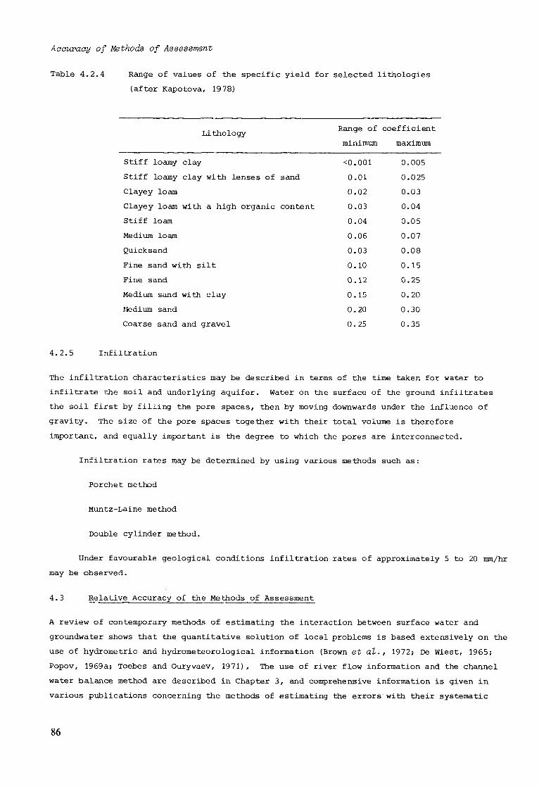
Aceuraoy of Methods of Assessment
Table 4.2.4 Range of values of the specific yield for selected lithologies
(after Kapotova, 1978)
T . ̂ , , Range of coefficient Lithology
Stiff loamy clay
Stiff loamy clay with le
Clayey loam
Clayey loam with a high
Stiff loam
Medium loam
Quicksand
Fine sand with silt
Fine sand
Medium sand with clay
Medium sand
Coarse sand and gravel
mses of
organic
sand
content
minimum
<0.001
0.01
0.02
0.03
0.04
0.06
0.03
0.10
0.12
0.15
0.20
0.25
maximum
0.005
0.025
0.03
0.04
0.05
0.07
0.08
0.15
0.25
0.20
0.30
0.35
4.2.5 Infiltration
The infiltration characteristics may be described in terms of the time taken for water to
infiltrate the soil and underlying aquifer. Water on the surface of the ground infiltrates
the soil first by filling the pore spaces, then by moving downwards under the influence of
gravity. The size of the pore spaces together with their total volume is therefore
important, and equally important is the degree to which the pores are interconnected.
Infiltration rates may be determined by using various methods such as:
Porchet method
Muntz-Laine method
Double cylinder method.
Under favourable geological conditions infiltration rates of approximately 5 to 20 mm/hr
may be observed.
4.3 Relative Accuracy of the Methods of Assessment
A review of contemporary methods of estimating the interaction between surface water and
groundwater shows that the quantitative solution of local problems is based extensively on the
use of hydrometric and hydrometeorological information (Brown et al., 1972; De Wiest, 1965;
Popov, 1969a; Toebes and Ouryvaev, 1971), The use of river flow information and the channel
water balance method are described in Chapter 3, and comprehensive information is given in
various publications concerning the methods of estimating the errors with their systematic
86

Accuracy of Methods of Assessment
and random components (Anon, 1977a; Popov, 1975; Sokolov and Chapman, 1974) . In addition
sections 4.1 and 4.2 discuss the problems associated with the accuracy of measuring runoff and
aquifer characteristics.
When examining the interaction process with the aid of available information and
conceptual models, some systematic errors.are likely to occur when comparing estimated and
observed groundwater levels and river flows. In most cases the determination of quantitative
estimates of the interaction is a very complicated problem.
4.3.1 Channel Water Balance
The availability and accuracy of field data has a strong influence on the reliability of the
channel water balance (CWB) calculation. The accuracy of the CWB calculation can be given in
terms of a mean quadratic value (the standard deviation) that incorporates the rather complex
errors arising from the computation of each element, ç., as shown in equation 4.3(1).
/i=n 2 fi™ C = J Ï C : = A 2 (d, Q H ) 2 4.3(1)
where d is the relative mean quadratic error (coefficient of variation) of discharge Q, and
n is the total number of the CWB components.
The relative errors, d, are determined for the elements of the CWB appropriate to the
methods adopted (Anon, 1977a; Anon, 1977c; WMO, 1965).
The results of the CWB computation are considered to be reliable if the absolute value
of the remainder term in the CWB equation is significantly different from the maximum error of
its determination.
I S> I » Œ Ç 4.3(2) 1 o ' p o
where Πis the p% confidence level from the error computation in terms of its mean
quadratic value, and p is the confidence coefficient or probability p.
For reliable estimates of the CWB computation, the minimum acceptable value of the
probability p may be given as p = 0.95, for which « = 2 . Therefore the criterion for a P
reliable CWB computation can now be written in-the form of the following inequality:
I Q 0 I > 2 C0 4.3(3)
or dQ $ 0.5 | Qo | 4.3(4)
For the case where relatively small changes in runoff occur in a reach, the accuracy of
computations depends mainly on the accuracy of discharge measurements at the upstream and
downstream cross sections. Errors in the other elements of the CWB should be neglected because
of their relatively small values. In this case the mean quadratic error of discharge
measurement in the reach (AQ) is estimated by the formula of Karasev:
87
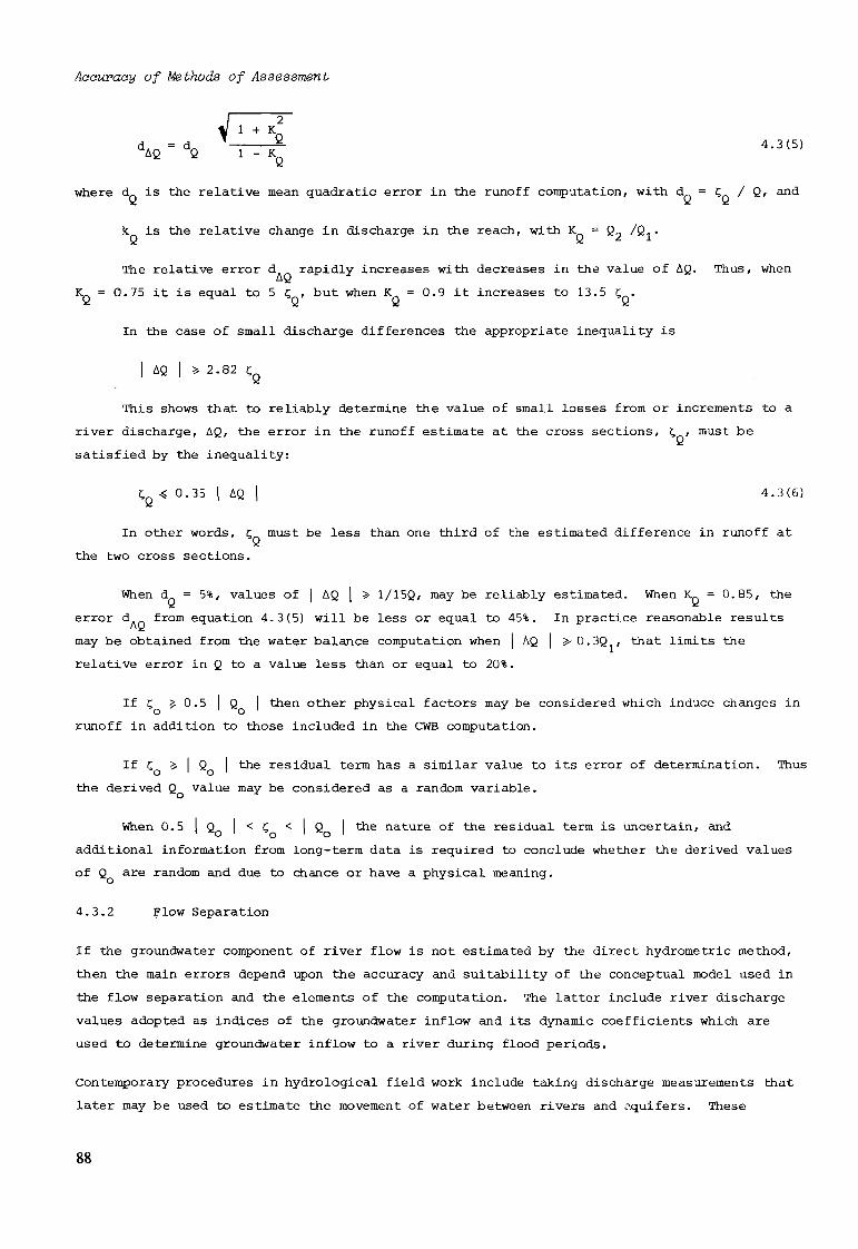
Accuracy of Methods of Assessment
V 1 + Kc 2
a - ̂ — - 2 - 4.3(5) AQ Q 1 - KQ
where d is the relative mean quadratic error in the runoff computation, with d = Ç / Q, and
k is the relative change in discharge in the reach, with K = Q9 /Q. . Q y ¿ i
The relative error d rapidly increases with decreases in the value of AQ. Thus, when
K = 0.75 it is equal to 5 ç , but when K = 0.9 it increases to 13.5 ç .
In the case of small discharge differences the appropriate inequality is
| AQ | » 2.82 ÇQ
This shows that to reliably determine the value of small losses from or increments to a
river discharge, AQ, the error in the runoff estimate at the cross sections, ç , must be
satisfied by the inequality:
ÇQ « 0.35 | AQ | 4.3(6)
In other words, ç must be less than one third of the estimated difference in runoff at
the two cross sections.
When d = 5%, values of [ AQ | » 1/15Q, may be reliably estimated. When K Q = 0.85, the
error d from equation 4.3(5) will be less or equal to 45%. In practice reasonable results
may be obtained from the water balance computation when | AQ | >0.3Q , that limits the
relative error in Q to a value less than or equal to 20%.
If Ç J- 0.5 | Q | then other physical factors may be considered which induce changes in
runoff in addition to those included in the CWB computation.
If ç 5- I Q I the residual term has a similar value to its error of determination. Thus o i o i
the derived Q value may be considered as a random variable.
When 0.5 Q I < ç < I Q I the nature of the residual term is uncertain, and 1 o ' o ' o '
additional information from long-term data is required to conclude whether the derived values
of Q are random and due to chance or have a physical meaning.
4.3.2 Flow Separation
If the groundwater component of river flow is not estimated by the direct hydrometric method,
then the main errors depend upon the accuracy and suitability of the conceptual model used in
the flow separation and the elements of the computation. The latter include river discharge
values adopted as indices of the groundwater inflow and its dynamic coefficients which are
used to determine groundwater inflow to a river during flood periods.
Contemporary procedures in hydrological field work include taking discharge measurements that
later may be used to estimate the movement of water between rivers and aquifers. These
88

Accuracy of Methods of Assessment
measurements have a specified accuracy (Ratner, 1970). However, to use the discharge values in
later computations, it is necssary to ascertain that river water is formed from groundwater
according to the assumptions inherent in the conceptual model. This should be done on the
basis of complementary information concerning the hydrometeorological and hydrogeological
regime.
In the absence of complete information about the groundwater regime, the quantitative
estimate of the local dynamic coefficients representing the groundwater inflow is rather
complicated. This is typically the case when hydrograph separation methods are used.
Improvements in the separation methods, and increased accuracy, must be based on studies of the
variations in space and time of the characteristics of the formation of groundwater inflow to
rivers. Thus correct allowances should be made for groundwater inflow from each major aquifer
and reach in the river basin under study.
4.3.3 Mathematical Models
There are several statistical measures that are used to describe the accuracy of mathematical
models and each of these measures can be influenced by physical and experimental factors.
In this section two measures of accuracy are discussed for rainfall-runoff models and their
relationship to various factors described based upon analyses for representative basins in
England and Wales (Wright, 1978). The examples are intended to give a general indication of
the factors that influence the accuracy of flow estimation and the important effect that basin
geology has on model accuracy.
The accuracy of equations relating river flows to weather data may be given in terms of
their residual error of estimate and the coefficient of multiple correlation. The residual
error is calculated from the difference between the measured and estimated flows for the
period of model.calibration and may be given in terms of a per cent of the flow. Thus an
equation with a residual error of 25 per cent would be expected to estimate flows within
50 per cent for 95 per cent of the time. Figure 26 shows the relationship between the residual
error, the coefficient of multiple correlation and flow variability for equations derived for
75 representative basins in England and Wales.
An equation relating rivers flows to weather data could have a residual error (E) of 25
per cent and a coefficient of multiple correlation (R) of 0.96 or 0.9 7 if the coefficient of
variation (C ) for monthly flows was between 0.3 and 0.4. The relationship between these
measures is given by equation 4.3(7).
E = C \1 - R2 4.3(7)
Table 3.5.7 indicates the rock types associated with specified values of flow
variability and weather conditions. Thus in areas with similar weather conditions and known
rock types it may be possible to estimate the probable accuracy of rainfall-runoff models
before equations have been derived. Rivers with a high proportion of groundwater flow will
tend to be characterised by relatively low values of flow variability because of the smoothing
89
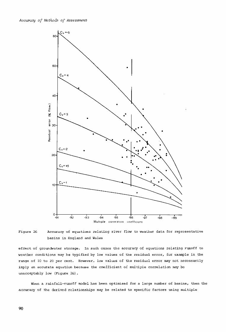
Accuracy of Methods of Assessment
Multiple correlation coefficient
Figure 26 Accuracy of equations relating river flow to weather data for representative
basins in England and Wales
effect of groundwater storage. In such cases the accuracy of equations relating runoff to
weather conditions may be typified by low values of the residual error, for example in the
range of 10 to 20 per cent. However, low values of the residual error may not necessarily
imply an accurate equation because the coefficient of multiple correlation may be
unacceptably low (Figure 26) .
When a rainfall-runoff model has been optimised for a large number of basins, then the
accuracy of the derived relationships may be related to specific factors using multiple
90

Accuracy of Methods of Assessment
regression techniques. For example the residual error (E) for equations to estimate river
flows in 55 representative basins in England and Wales has been related to several factors as
shown in equation 4.3(8) .
16300 C - 9 5 O'11
E = 4.3(8) l A G - 0 7 * * ! - 1 7 ™ - 1 8
where C is the coefficient of variation of monthly flows (range 0.1 to 0.6, examples given
in Table 3.5.3)
C is the length of the model calibration period, in months (range 60 to 1000 months),
LAG is the maximum significant lag in the equation in months (range 1 to 18 months),
RAI is the number of rainfall stations used to estimate mean catchment rainfall
(range 3 to 27) ,
RIV is the type of flow measuring station, 1 represents a calibrated river section,
2 a structure in the river not designed specifically for flow measurement and 3 a
structure designed for flow measurement.
All the coefficients for the five independent variables were significant at the 5 per
cent level, and the equation accounted for 84 per cent of the variance in the residual error.
The single most important independent variable is flow variability (C ), which accounts for
75 per cent of the total variance in the residual error.
Although equation 4.3(8) is limited in application to a part of western Europe, the
accuracy of other types of model may be expected to be subject to similar factors. For
example accuracy may depend upon:
1. Variability of the dependent variable such as groundwater levels or river flows,
2. Length of the model calibration period,
3. The lag effect of storage at the surface, in the unsaturated zone or in the
saturated zone,
4. The sampling density or number of sampling points for variables such as rainfall
or groundwater levels,
5. Accuracy of measuring or estimating the variables such as rainfall, evaporation,
groundwater levels and flow.
The use of remote sensing from aircraft and satellites may be used to improve the
accuracy of estimating certain components of the hydrological cycle such as the areal extent
of aquifers, wetlands, saturated soils, irrigation and types of land use and vegetation cover
(Moore, 1979). Of particular interest for modelling purposes is the use of radar for
91

Accuracy of Methods of Assessment
estimating the areal extent, duration and intensity of rainfall (Browning et al., 1977). The
extreme variability of thunderstorm rainfall is well known, but even widespread frontal rain
can include areas of substantially heavier rain. Thus radar is being developed to improve the
accuracy of areal rainfall estimates and this has some potential as an aid for assessing water
resource schemes in both temperate and arid regions. The areal coverage of rainfall stations
tends to be rather sparse in some parts of the world such as the tropical forest, desert and
mountainous regions of Asia, Africa and South America, although a better coverage often exists
along valleys (Anon, 1978).
In conclusion the accuracy of a mathematical model will depend upon how adequately the
components of the hydrological cycle are represented by mathematical equations. Thus
improvements in assessing the interaction between surface water and groundwater will depend
upon improving techniques for measuring the variables and improved modelling procedures
including a better understanding of the interaction process.
92
Case Studies
5. Case studies 5.1 Temperate Area: Great Ouse Pilot Scheme, UK
5.1.1 Introduction
Increasing effort has been directed in water resource development in England and Wales to make
more efficient use of groundwater stored in the Chalk and Triassic sandstones. One method
designed to achieve this objective is to regulate river flows by means of the intermittent
abstraction of groundwater to enable a relatively high river abstraction to be sustained at a
downstream point on the river system. This method of development maintains riverside amenities*
safeguards navigation interests and maximises the yield by utilising both surface runoff and
groundwater storage. The variability of river flows is reduced by the redistribution in time
of the groundwater component of river flow. In such schemes it is. essential to examine the
interaction of surface flow and groundwater to minimise both capital and operational costs.
The number and location of abstraction wells must be carefully designed to ensure that river
flows are adequately augmented in dry years to support the design yield.
Several experimental areas have been set up to examine the feasibility of regulating
river flows by the intermittent abstraction of groundwater. Groundwater abstraction losses in
pilot schemes have been estimated (Wright, 1974) and ascribed to either (a) pumped
intercepted base flow or (b) induced river bed infiltration (Kemp and Wright, 1977). This case
study describes some of the work carried out in the Thet pilot scheme in Norfolk. Figure 27
shows the mean annual rainfall less actual evaporation over a part of south-east England,
the Chalk and the Thet pilot scheme area.
Test pumping programmes for the 18 abstraction wells (Figure 28) were carried out
between 1968 and 1971 to determine the well and aquifer characteristics and provide some 2
practical experience in river regulation by groundwater. The pilot scheme area covers 71.5 km ,
varying in height from 15 m to 50 m above mean sea level. The land is mainly arable with some
forest and heath, and soils are free draining. A summary of the work carried out in the Great
Ouse pilot scheme area was described by Backshall et al. (1972), and due to the success of the
experiment proposals for development were outlined (Great Ouse River Authority, 1972).
93
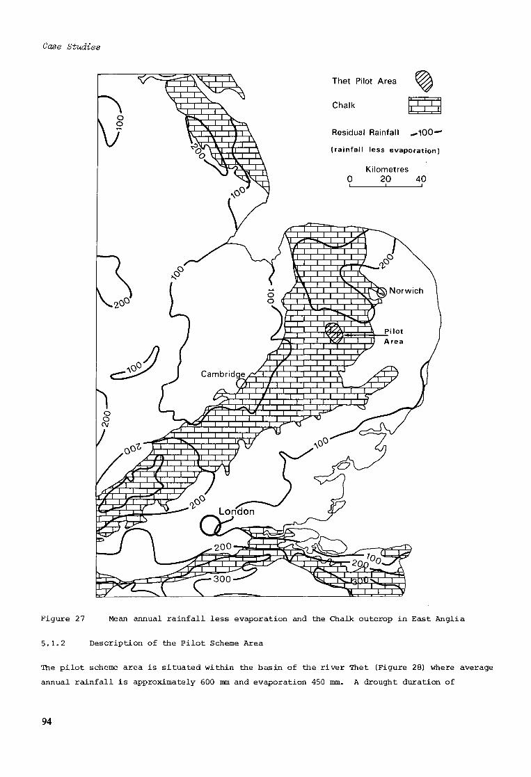
Case Studies
Thet Pilot Area
Chalk ' 1 ' 1 ' i i i
Residual Rainfall - .100—'
(rainfall less evaporation)
Figure 27 Mean annual rainfall less evaporation and the Chalk outcrop in East Anglia
5.1.2 Description of the Pilot Scheme Area
The pilot scheme area is situated within the basin of the river Thet (Figure 28) where average
annual rainfall is approximately 600 mm and evaporation 450 mm. A drought duration of
94

Case Studies
Thet Pilot Area • •
Gauging station V
Abstraction wells ®
Met. station 0
Kilometres 0 1 2 . 3
/ V»
S
<
I
\
t I
/
J
Figure 28 Thet groundwater Pilot Scheme
approximately 9 months is that which tends to be critical to the maintenance of water supplies
(a) in eastern England from small and medium surface reservoirs, and (b) from groundwater
storage such as that required to maintain flows in the river Thet at 50 per cent of the annual
mean value throughout a 1 in 50 year drought event. If greater use is made of groundwater
storage by maintaining river flows at a higher proportion of the mean, then minimum ground
water levels during a 1 in 50 year drought would tend to occur after 18 or 30 months,
similar to the critical duration for larger surface reservoirs (Downing et dl., 1973).
There are five flow gauging stations on the river Thet and its tributaries, four of
which measure flows into and out of the pilot area. The fifth gauge, at Melford Bridge, is
downstream of the pilot area and has the longest record. It is a triangular profile weir
specially designed for flow measurement and constructed in 1962. The drainage area to this 2
gauge is 316 km . Table 5.1.1 contains the average rainfall, evaporation and river flow
components for the basin to Melford Bridge. Groundwater flow in the river Thet is commonly a
high proportion of the total flow during the summer six months, April to September.
95

Case Studies
Table 5.1.1 Mean rainfall, evaporation and river flow components : River Thet to Melford
Bridge (mm)
Rainfall
Evaporation
Total flow
Base flow
Jan
57
6
31
11
Feb
43
10
28
13
Mar
39
18
24
14
Apr
48
32
19
13
May
46
60
13
11
Jun
45
78
9
7
Jul
65
78
6
5
Aug
59
70
5
4
Sep
57
50
5
4
Oct
59
23
8
4
Nov
64
15
15
6
Dec
55
10
23
8
Annual Total
637
450
187
100
The bed rock in the pilot area is the Upper Chalk which is overlain in places by super
ficial deposits comprising mainly sands and gravels or Chalky Boulder Clay. The geological
succession is given in Table 5.1.2, and a brief description is given of the characteristics of
the alluvium, boulder clay and the Chalk.
Table 5.1.2 Geological Strata in the Thet Pilot Scheme area
Period Stratigraphie Unit Approximate maximum
thickness (m)
Recent Blown sands
Alluvium
Terrace deposits
Pleistocene Loam
Boulder clay
Sand and gravel
5
30
15
Cretaceous Upper Chalk
Middle Chalk
Lower Chalk
Gault
120
70
60
65
Alluvium deposits occur along the flood plain of the rivers. The alluvium has a
variable lithology reflecting the properties of the nearby Pleistocene deposits of Boulder
Clay and sand and gravel. Much of the higher ground and parts of the valleys are covered by
Boulder Clay, which is a stiff clay with a variable lithology. Infiltration to the Chalk is
reduced beneath the Boulder Clay due to its relatively impermeable nature, and groundwater in
the Chalk tends to be confined in these areas.
Areas of bare ChdUi crop out along the sides of valleys between the Boulder Clay on the
hills and the valley alluvium. The Chalk is a soft white fine grained limestone composed
almost entirely of organic remains. Although it has a porosity of between 25 and 40 per cent
the pore spaces are very small and the mean flow of water occurs along joints, fissures.
96

Case Studies
bedding planes and flint surfaces. The size of fissures generally reduces with depth and
most groundwater is obtained from the top 30 m of the aquifer, although individual hard beds
of rock below this may contribute significant supplies. The transmissivity varies from less 2 2 2
than 10 m /day below the high ground to between 750 m /day and 1500 m /day or more at favourable localities in the valleys. Values for the specific yield are generally between
1.0 and 3.0 per cent.
The Chalk is subdivided into three divisions, the Lower, Middle and Upper Chalk.
Groundwater levels fluctuate within the Upper Chalk or in the overlying drift. At the base of
the Upper Chalk there are hard bands of rock up to 8 m thick which are an important water
bearing horizon- Likewise, a hard band of rock exists at the base of the Middle Chalk. The
Lowev Chalk is generally less favourable for groundwater development.
5.1.3 Measurements
Sub-surface geophysical work in connection with the Pilot Scheme was begun in 1967 with the
objective to determine the physical properties of the Chalk, the correlation of the strata
between the wells and the study of groundwater quality. A resistivity survey was run to a
depth of 180 m in the deepest available borehole with measurements at 1 m intervals. The log
obtained was later used to interpret resistivity logs from the 18 abstraction wells.
Measurements of electrical conductivity and temperature confirmed that the quality of the water
did not change with depth. In addition the following logs were run:
spontaneous potential continuously recorded
single electrode resistance continuously recorded
multiple electrode resistivity 0.5 m readings
Gamma ray continuously recorded
Caliper continuously recorded
Spinner flowmeter selected intervals
In the western part of the pilot area the final depths of the abstraction wells are
related to the base of the Upper Chalk, and the final depths of the wells were controlled by
the use of electric logs.
The hydrometric network was established in two stages. The first stage was
substantially completed by the end of 1967 and involved the drilling of 24 observation bore
holes of 153 mm diameter, the construction of five river flow gauges, and the installation of
eight rain gauges. The second stage included drilling a further 56 observation boreholes,
constructing a further six flow measuring points on springs and tributaries and building a
climate station near the centre of the area. The flow was measured from each abstraction well.
97

Case Studies
5.1.4 Natural River Flow and Groundwater Level Relationship
Measurements were made of river flows and groundwater levels prior to the start of groundwater
abstraction so that flow and level relationships could be derived for natural conditions.
Ideally at least two years of such records should be available to enable accurate
relationships to be derived for use in assessing the effects of groundwater abstraction.
Methods used to assess the effects of pumping included:
1. cross correlation of river flows,
2. rainfall-runoff models relating river flows to weather data,
3. aquifer characteristics, and
4. analogue model of groundwater flow.
The most accurate method of assessing the change in river flow due to groundwater
abstraction was found to be that based upon the cross correlation of river flows (Wright, 1974).
Measured and estimated natural river flows based upon this method are shown in Figure 29;
based upon five day means.
River flows may also be estimated from weather data. A monthly rainfall-runoff
regression model has been optimised for many basins in England and Wales (Wright, 1978), and
one of the basins examined was the river Thet to Melford Bridge. The derived rainfall-runoff
equation for this basin has a coefficient of multiple correlation of 0.984 and a residual error
of 15 per cent of the flow. During average weather conditions a positive increment of
rainfall less evaporation falling over the basin will continue to significantly influence river
flows for 14 months after the event due to the large groundwater storage in the Chalk. A
typical response of river flow to 10 mm of rainfall less evaporation is shown in Figure 30.
Rather more than 30 per cent of the basin comprises semi-permeable boulder clay overlying
the Chalk. This accounts for the rapid response of river flow to rainfall during wet weather.
When the soil is below field capacity a positive value of rainfall less evaporation has a
maximum effect upon river flows approximately one month after the rainfall event.
The analysis of river hydrographs and groundwater levels provided estimates of the
coefficient of storage using the following method. During long periods of dry weather the
river flow recession curve may be written as equation 3.2(5) which is:
Q t = Ô 0e - Œ t 5.1(1)
and after integration becomes:
S t = — 5.1(2)
The relationship between mean basin groundwater levels and base flow may be written as:
W = a + bF 5.1(3)
98

Case Studie
a) G R O U N D W A T E R ABSTRACTION
_ 0.5 -
5 o
1.5
1.0
5 o
0.5
b) R IVER F L O W
I I
I ' 1_J target
regulation
flow
f low
augmentation
estimated natural flow
T T Sept May July Nov
1 971
Figure 29 Regulation of river flow at Bridgham by groundwater, 1971
By definition the coefficient of storage is the change in volume of stored groundwater
divided by the change of groundwater levels during the same period, thus:
st - St Cl 2 S = x 100%
1 2 5.1(4)
Combining equations 5.1(3), 5.1(4) and 5.1(5) we obtain:

Case Studies
2A 1 0 m m of residual rainfall (rainfall less evaporation)
Figure 30 Response of river flow to rainfall less evaporation at Melford Bridge
If the water levels are in metres and the base flow is in millimetres of runoff for a
period of one month/ and the dry weather flow approximates to the base flow, then equation
5.1(6) reduces to:
S = 0.00329
°<b 5.1(6)
where Q and Q are the flows at time t and when t = o respectively,
S is the volume of groundwater in active storage at time t,
W is the mean basin groundwater level
S is the coefficient of storage
F is the mean monthly base flow
and e, Π, a and b are constants.
An analysis of the base flow and groundwater levels in the Thet catchment gave a value
of b = 0.19 in equation 5.1(3) , and a dry weather flow recession constant of = = 0.0113 in
equation 5.1(1). Using these values in equation 5.1(6) the storage coefficient was
calculated to be 1.5% which agreed with values derived by other methods.
An electrical analogue model was constructed of the Pilot Area and the surrounding
region based upon the analogue between Ohm's Law and Darcy's Law. The system was modelled as 2
a slow-time resistance-capacitance network covering an area of 1050 km . Resistor elements
simulated transmissivity and capacitative elements simulated the storage properties of the
Chalk. The average groundwater levels were modelled by simulating the annual average values
of infiltration and the variation in transmissivity within the aquifer. The response of the
model suggested that the storage coefficient varied from 3% where the Chalk crops out to
100
Case Studies
0.05% where the groundwater is confined by extensive boulder clay cover, giving an average
value for the area of 1.5%.
The analogue model enabled many pumping programmes to be investigated, and examined the
effect of inflow of groundwater into the Pilot Area during periods of maximum drawdown. In
regional developments this inflow would tend to reduce due to drawdown also occurring in
adjacent areas.
5.1.5 Analysis of Group Pumping Tests, 1971
During 1971 the groundwater abstraction rate was varied to regulate river flows at Bridgham to
predetermined rates, as shown in Figure 29. This method of river regulation increases low
flows and reduces flood peaks. Early in May the measured flows were similar to the estimated
flows indicating that the depressions in the groundwater table made by abstractions the
previous year had been substantially filled by the natural winter recharge. Later on in May
and June the groundwater abstraction was increased to keep the river flow at Bridgham near to
the initial regulation rate of 1000 1/sec. Minor floods in June and early August enabled
groundwater abstraction to cease from most wells for a day or two. At the beginning of each
day the flows at Redbridge and Bridgham were examined and the number of pumping wells
determined. The travel time of pumped groundwater discharges reaching Bridgham varied from
1 hour for nearby wells to 7 hours for those most distant, representing on average an effective
river flow velocity of 2 km/hr.
The pumping pattern in 1971 can be considered to comprise three stages separated by
prolonged periods of rain. During the first period which extended up to 9 June, the average
pumping rate was 300 1/sec and the average gain in flow 150 1/sec. The difference comprised
groundwater that was pumped which would naturally have found its way to the river as base flow.
Pumping in this period was mainly from wells at some distance from the main river channels
therefore induced infiltration through the river bed would have been negligible (Kemp and
Wright, 1977).
The second period of pumping, from 22 June to 27 July involved pumping 15 of the 18 wells
for much of the time. The net gain in flow generally varied between 70 to 80% -of the
abstraction rate which was similar to that for the third period which ended on 12 October.
Induced river bed infiltration probably did not exceed 10% of the groundwater abstraction.
Higher losses could have occurred during the 1970 tests when groundwater levels were lowered
below the river bed along several reaches.
Extensive tests in a number of pilot schemes have shown the economic advantages of care
ful selection of sites for abstraction wells. In areas where the river bed is relatively
impermeable wells may be sited close to the river to take advantage of the higher coefficients
of storage in such areas and reduced capital costs due to short pipelines to the river. Where
the river bed is permeable the wells have to be sited some distance from watercourses to avoid
induced river bed infiltration.
101

Case Studies
5.2 Temperate Area: The Moscow Artesian Basin, USSR
5.2.1 Introduc tion
This case study describes the interaction between river water and groundwater in the Moscow
Artesian Basin which is an area with intensive groundwater development. The groundwater regime
of the basin represents a complicated hydrodynamic system with the considerable groundwater
abstraction reducing groundwater runoff and modifying the natural interaction between ground
water and surface water.
In temperate climates a typical characteristic of the interaction is the groundwater
inflow to rivers. However high levels of groundwater development generally deplete both the
groundwater inflow (base flow) and the total runoff. Where the groundwater abstraction has
created a cone of depression that extends to the river channel runoff may be reduced also by
the loss of river water to groundwater. However the return of groundwater abstractions to
rivers will increase runoff in those areas where the groundwater would not otherwise have
contributed to runoff. Estimates are required of such changes in the natural interaction
between groundwater and river water to solve problems associated with hydrological aspects of
multi-purpose water resource schemes that include groundwater development.
5.2.2 The Moscow Basin
An analytical solution has been described by Minkin and Kontsebovsky (1979) to estimate the
decrease in runoff due to the effect of specified major groundwater abstractions. However the
solution for the Moscow basin is complicated by several factors such as the regional nature
of the problem caused by the extensive network of abstraction wells and the availability of
detailed hydrogeological information. Moreover an adequate account has to be taken of the
variation in runoff caused by the return of groundwater to rivers after for example domestic
or industrial use.
The regional assessment of the interaction between surface water and groundwater, and the
prediction of variations in runoff due to the effect of intensive groundwater development,
should be obtained by the analysis of hydrometric data (Anon, 1973b; Anon, 1974). Thus
artificial changes in runoff may be assessed by taking the difference between the measured
river flow and the estimated natural flow. To illustrate this method of investigating the
interaction some analyses are presented for the Moscow Artesian Basin.
The region under investigation has a temperate climate and lies near the centre of the
Eastern European plain. The countryside is typically undulating with hills, valleys, moraine
ridges and lowland areas, and is at the centre of the Moscow Artesian Basin. This basin is
hydrogeologically complex with aquifers that are drained by a network of surface channels that
have developed in the zone of intensive water exchange associated with the Quaternary and
Mesozoic deposits (Lebedeva, 1972).
102

Case Studies
5.2.3 Analyses
Base flow in this area is typically associated with a backwater type of regime as described in
section 3.2.1 and Figure 2. There is a relatively small variation in base flow during a year.
The effect of man's activities, in particular the intensive and substantial groundwater
development, has changed the hydrological regime of the river basins. Thus there now exists
the problem of determining the natural groundwater resources of the region and substantiating
the future safe groundwater yield based upon the available data. To solve this problem
required the estimation of the groundwater inflow to the rivers, together with the associated
inflow parameters and the determination of the difference between the measured river flows and
the estimated natural runoff.
Groundwater inflow values were obtained for successive reaches of the drainage basins by
analysing the measured long-term runoff data, supplemented by low flow measurements taken as
part of hydrometric surveys during notable historic dry periods. From this information the
long-term annual groundwater inflow values also were obtained (Ratner, 1978). The careful
location of river gauging stations, based upon hydrometric surveys, enables due account to be
taken of hydrogeological features that influence the formation and characteristics of ground
water inflow.
Annual values of the groundwater inflow were obtained using a simplified method based
upon low flow data recorded during the summer and winter low flow periods. This method is
suitable for those cases where there is a relatively small variability in groundwater runoff.
The groundwater runoff characteristics of the zone under consideration can be determined from
an examination of the relevant hydrogeological data (Popov, 1972).
Values of the natural groundwater inflow were estimated for those reaches with a
disturbed river flow regime caused by the effect of groundwater abstraction. Methods used to
reconstruct the river flow hydrograph included correlation, multiple correlation, channel water
balance and hydrological analogy. The method used for specific cases depended upon the
available data and the extent to which the natural regime, relating to the interaction between
groundwater and river water, was changed by man's actions (Ustiuzhanin, 1974). All the above
methods were used in deriving the probability distribution of the long-term groundwater inflow.
The deviations of the estimated actual groundwater inflow from the reconstructed natural
values for each water year were assumed to be equal to the change in the groundwater inflow
caused by groundwater abstraction.
This method may be applied to assess the natural groundwater resources in areas where
man has changed the natural interaction processes between river water and groundwater. Also
due account may be taken of the variations in groundwater inflow caused by intensive ground
water development. Thus up-to-date estimates can be made of variations in river flow caused
by reduced groundwater inflow or by the infiltration of river water to cones of depression in
the water table aaused by groundwater abstraction. The latter is applicable to specific
regions near industrial cities as shown in Table 5.2.1. The generalised regional situation
illustrating the disturbance to natural groundwater inflow to rivers in the central part of
103

Case Studies
the Moscow Artesian Basin is shown in Figure 31.
Table 5.2.1 Reduction in runoff caused by depressed groundwater levels in selected reaches
of rivers near industrial cities in the Moscow Artesian Basin
River
1
Kliazjma
Kliazjma
Pakhra
River Reach
2
near Noginsk
near Orekhovo-
zouevo
near Podolsk
Year
3
1970
1971
1970
1971
1970
1971
Basin Area
(km2)
4
210
210
2360
2360
1310
1310
Length of
reach
(km)
5
10.0
10.0
37.2
37.2
25.2
25 .2
reduced ground
water inflow
(m3/s)
6
0.6
0.45
0.80
2.50
1.40
0.70
Reduction in r
river water
infiltration
(m3/s)
7
0.2
0.65
0.00
0.00
0.44
1.18
unof f
total reduction
(m3/s)
6+7=8
0.80
1.10
0.80
2.50
1.84
1.88
(1/s.km2)
8-4=9
3.8
5.2
0.3
1.1
1.4
1.4
(1/s.km)
8*5=10
80.0
110.0
21.5
67.0
73.0
75.0
Moscow near 1971 4300 Lytkarino and Bronnitsy
54.0 10.0 2.3 185.0
Moscow near Kolomna
1971 2100 18.0 (8.3) (4.0) (460.0)
Kliazjma near Kovrovo
1972 3800 16.0 2.0 0.0 2.0 0.5 125.0
Within the area under consideration two main regions may be identified where there are
substantial disturbances to the natural interaction between groundwater and river water. These
two regions are within the influence of the so called 'Moscow' and 'Meshcherskij' depressions
in the water table caused by intensive groundwater development. At the present time in the
Moscow region the groundwater inflow to rivers is reduced by 20-35% of the annual natural
value, and the annual total runoff is reduced by 5-25%. The corresponding values for the
second region are 25-60% and 10-25% respectively. A comparison of these changes in runoff with
the rates of groundwater abstraction in the respective basins proves the decisive influence
that groundwater development has on these changes in runoff.
5.2.4 Future Situation
By the year 2000 the two regions are predicted to be within the area of a major depression in
the groundwater table caused by continued intensive groundwater development (according to
V.S. Plotnikov) . Therefore it is necessary to estimate a safe level of groundwater development
104

Case Studies
Key 1 Regional decrease in groundwater inflow 2 Increased runoff due to effluent discharges 3 Predicted regional lowering of groundwater table from the year 1980 to 2000 4 River reaches with reduction of groundwater inflow 5 River control sections 6 Reduction of groundwater flow as percentage of annual mean
Figure 31 Disturbance of groundwater inflow to rivers in the central part of the Moscow
Artesian Basin (after B.S. Ustiuzhanin)
for the whole of the Moscow Artesian Basin. Because the methods described are reasonably
accurate, they are used to estimate possible changes in runoff and regional changes in the
interaction between groundwater and river water. Thus the methods should be the basis for
organising future hydrological and hydrogeological investigations to enable an adequate assess
ment to be made of the impact of various water resource projects.
105
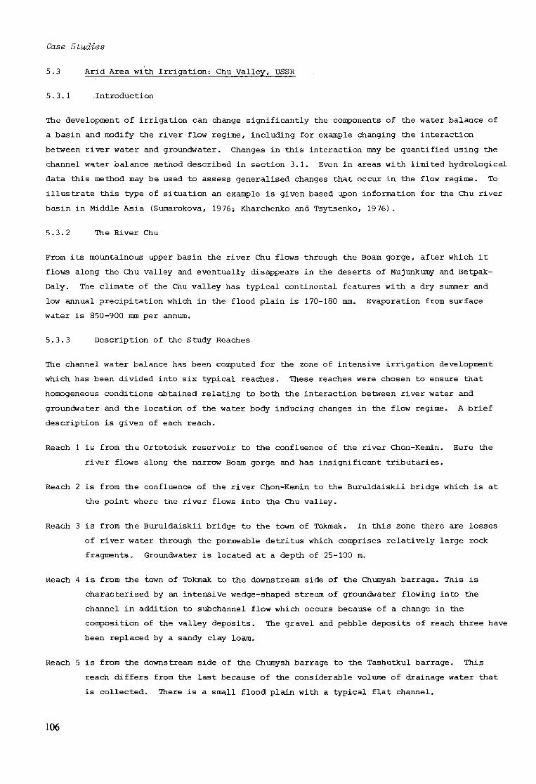
Case Studies
5.3 Arid Area with Irrigation: Chu Valley, USSR
5.3.1 . Introduction
The development of irrigation can change significantly the components of the water balance of
a basin and modify the river flow regime, including for example changing the interaction
between river water and groundwater. Changes in this interaction may be quantified using the
channel water balance method described in section 3.1. Even in areas with limited hydrological
data this method may be used to assess generalised changes that occur in the flow regime. To
illustrate this type of situation an example is given based upon information for the Chu river
basin in Middle Asia (Sumarokova, 1976} Kharchenko and Tsytsenko, 1976).
5.3.2 The River Chu
From its mountainous upper basin the river Chu flows through the Boam gorge, after which it
flows along the Chu valley and eventually disappears in the deserts of Mujunkumy and Betpak-
Daly. The climate of the Chu valley has typical continental features with a dry summer and
low annual precipitation which in the flood plain is 170-180 mm. Evaporation from surface
water is 850-900 mm per annum.
5.3.3 Description of the Study Reaches
The channel water balance has been computed for the zone of intensive irrigation development
which has been divided into six typical reaches. These reaches were chosen to ensure that
homogeneous conditions obtained relating to both the interaction between river water and
groundwater and the location of the water body inducing changes in the flow regime. A brief
description is given of each reach.
Reach 1 is from the Ortotoisk reservoir to the confluence of the river Chon-Kemin. Here the
river flows along the narrow Boam gorge and has insignificant tributaries.
Reach 2 is from the confluence of the river Chon-Kemin to the Buruldaiskii bridge which is at
the point where the river flows into the Chu valley.
Reach 3 is from the Buruldaiskii bridge to the town of Tokmak. In this zone there are losses
of river water through the permeable detritus which comprises relatively large rock
fragments. Groundwater is located at a depth of 25-100 m.
Reach 4 is from the town of Tokmak to the downstream side of the Chumysh barrage. This is
characterised by an intensive wedge-shaped stream of groundwater flowing into the
channel in addition to subchannel flow which occurs because of a change in the
composition of the valley deposits. The gravel and pebble deposits of reach three have
been replaced by a sandy clay loam.
Reach 5 is from the downstream side of the Chumysh barrage to the Tashutkul barrage. This
reach differs from the last because of the considerable volume of drainage water that
is collected. There is a small flood plain with a typical flat channel.
106

Case Studies
Reach 6 is from the downstream side of the Tashutkul barrage to the village of Furmanovka.
The characteristics are similar to those of reach five. Below Furmanovka the river
flows in the direction of the Aral Sea and disappears in sand.
5.3.4 The Channel Water Balance
The channel water balance of the separate reaches is computed by analysing the river flow data
for the upstream and downstream sections of the reach. Hydrometrie data and abstractions are
available for the period 1911-1973. Precipitation on the water surface and evaporation have
been considered to be practically equal. To reduce the effect of random errors in estimates
of some of the water balance components, the computation has been completed to show the main
characteristics based upon average values for successive five year periods. The results are
shown in Table 5.3.1. The channel water balance for the study period enables the following
conclusions to be made for each reach concerning the characteristics of the interaction
between river water and groundwater.
In reaches one and two there are alternating periods of groundwater inflow and outflow,
generally within the limits ..of 1—3 m / s . These flows are relatively small and close to the
errors associated with the discharge measurements for the reaches.
In the third reach there are relatively substantial losses to groundwater of 17-33 m /s .
The data from recent years have shown losses to be generally lower than in earlier years. This
is due to augmented river abstractions that have decreased the mean discharge of the reach.
There is a sustained groundwater inflow to the river in reach four with maximum values
coinciding with periods of maximum river water abstraction and the relatively wet ten year
period 1950-1960. The augmentation of groundwater inflow in such periods apparently reflects
the increasing volume of return water from irrigated areas.
In reach five there is an overall tendency for groundwater inflow to be augmented with
increasing irrigation. A considerable increase of groundwater inflow has been observed with
the opening of the West Great Chu canal. Although there has been an increase in irrigated
areas over the last two decades this has coincided with a more rational use of water for
irrigation. Thus from 1960 there has been a tendency for groundwater inflow to decrease even
during relatively wet years such as 1969 and 1970 (Sumarokova, 1976).
During the period under consideration stream flow losses in reach six have been modified
by increments of groundwater inflow from returned irrigation water.
5.3.5 Summary
By examining the information in Table 5.3.1 it is apparent that during the period of study
certain trends have occurred in the data that quantify the interaction process. The total
groundwater losses in all reaches have decreased from 40 to 22 m /s. During the same 63-year
period the total groundwater inflow, including returned irrigation water, increased from 3 3 3
23 m /s in 1911-1915 to a peak of 67 m /s in 1956-1960 after which it decreased to 33 m /s by
107

Case Studies
1971-1973. The errors associated with these estimates as 25-35% according to Karasseff
(In Anon, 1977a).
Table 5.3.1 Tabulated values of groundwater inflow and losses for selected reaches of the
river Chu, 1911-73
Reach
1
2
3
4
5
6
Losses
Gains
1911-15
3.42
1.30
-32.1
18.4
-0.50
-7.98
40.6
23.1
Mean gain (+) or Loss (-)
1916-20 1921-25 1926-30
0.60 1.30
-12.4
in period
1931-35
3.22
1.30
-33.7
15.7
4.05
-8.10
41.8
24.3
(m3/s)
1936-40
2.47
-0.70
-26.2
20.4
-3.37
-8.27
38.5
22.9
1941-45
2.10
0.42
-28.2
18.2
7.56
-7.93
36.1
28.2
Reach
1
2
3
4
5
6
Losses
Gains
1946-50
-1.00
0.10
-27.5
20.4
13.2
-10.5
39.0
33.7
Mean gain
1951-55
-0.67
1.39
-30.5
42.9
16.5
4.61
31.2
65.4
(+) or Loss
1956-60
1.02
-1.54
-24.4
33.2
23.7
9.73
25.9
67.6
(-) in
1961-65
-1.45
-2.52
-17.0
24.3
12.1
9.80
21.0
46.2
period (m /s)
1966-70
-3.67
-0.25
-17.6
29.4
10.3
15.0
21.5
54.7
i
1971-73
-3.97
-0.50
-17.7
14.6
11.0
6.53
22.2
32.1
Although parts of the channel water balance compilation described in this study are
approximate, nevertheless they are of considerable practical importance. In particular they
have become the basis of more detailed water balance studies for the Chu river basin to
establish the influence of irrigation schemes and the effect upon water resources of changes
in the flow regime. Moreover, the analyses relating to the interaction process have already
enabled a number of practical measures to be adopted for the more rational use of water
resources in the Chu valley. For example in areas where a significant loss of water has been
identified through the permeable detritus, these losses may be reduced to zero by facing the
channel with concrete. This case study shows that the channel water balance method may be used
with standard hydrometric data to quantify the interaction between groundwater and surface
water, without necessarily any special field investigations.
108

Case Studies
5.4 Arid Area: Groundwater Replenishment by Surface Water, Tunisia
5.4.1 Introduction
This case study is an example of aquifer replenishment from surface runoff in an arid region
and is for the plain of Kairouan in Tunisia (Besbes et al., 1978). The plain of Kairouan 2
has the largest groundwater storage in central Tunisia, with a surface area of 3 000 km . It
is replenished mainly by flood water from two ephemeral streams the wadis Zeroud and
Merguellil. Flood waters in this internal drainage basin spread out and infiltrate to the
groundwater table then flow to the sebkhas which are natural depressions with brackish water
and evaporate. The annual potential evaporation of 1 500 mm substantially exceeds the mean
annual rainfall of 300 mm.
5.4.2 Aquifer Recharge in the Kairouan Plain
The upper aquifer comprises a concave depression that has been filled with lenticular
Pliocene - quaternary detritus which is more than 500 m thick, in which the phreatic ground
water surface covers the entire plain. However, there exists a second aquifer at depth which
is contained within a semi-permeable Quaternary formation.
Recharge areas around the boundary of the plain provide a common intake area to both
aquifers. Figure 32 shows the groundwater levels in the Kairouan plain, with the higher levels
associated with the wadis Zeroud and Merguellil. This confirms that recharge occurs
preferentially in these areas. Although the low flows of these two wadis completely infiltrate
on reaching the plain, an examination of the movement of groundwater levels and surface runoff
events over a period of several years shows that the floodwaters play a major role in
replenishing the groundwater (Figure 33) .
Annual runoff from the Zeroud and Merguellil wadis that infiltrates to the groundwater 6 3 6 3
table in the Kairouan plain is estimated to average 12 x 10 m and 7 x 10 m respectively, 6 3
whereas direct recharge from rainfall is estimated as 6 x 10 m per annum over an area of
1 000 km .
5.4.3 Recharge by Surface Runoff from the Zeroud Wadi
The determination of effective increases in groundwater levels resulting from floods will be
described for the period of 18 months from January 1968 to June 1969. Most of the 23
piezometers in the network recorded changes in the groundwater level corresponding to the
passage of four flood events. These floods were measured at the river gauging station at Sidi
Saad during the following months:
6 3 1 February to April 1968, 15 x 10 m
6 3 2 June 1968, 54 x 10 m
6 3 3 September 1968, 4 x 10 m
6 3 4 April to May 1968, 7 x 10 m
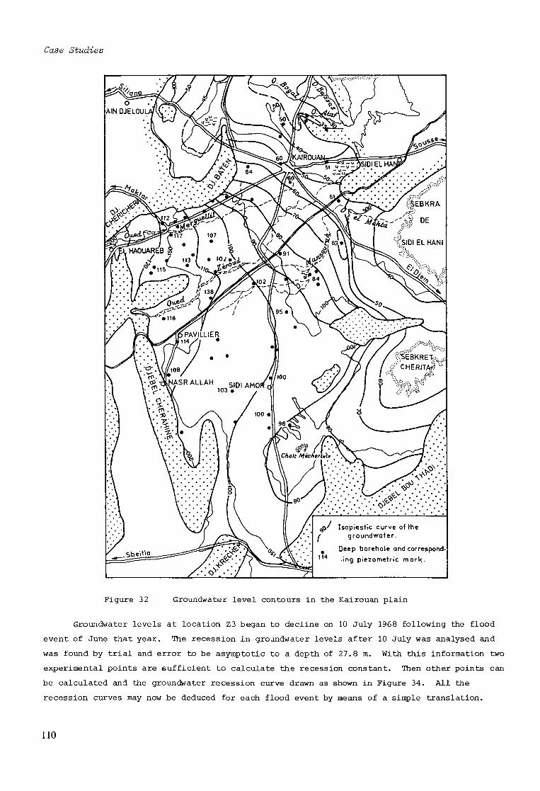
Case Studies
Figure 32 Groundwater level contours in the Kairouan plain
Groundwater levels at location Z3 began to decline on 10 July 1968 following the flood
event of June that year. The recession in groundwater levels after 10 July was analysed and
was found by trial and error to be asymptotic to a depth of 27.8 m. With this information two
experimental points are sufficient to calculate the recession constant. Then other points can
be calculated and the groundwater recession curve drawn as shown in Figure 34. All the
recession curves may now be deduced for each flood event by means of a simple translation.
110
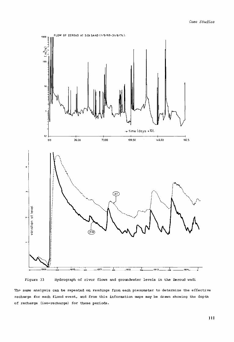
Case Studies
FLOW OF ZEROUD AT SIDI SAAD (1/9/69-31/8/74).
"E_
w^ time (days x10).
oo 36.50 73.00 109.50 146.00 182.5
Figure 33 Hydrograph of river flows and groundwater levels in the Zeroud wadi
The same analysis can be repeated on readings from each piezometer to determine the effective
recharge for each flood event, and from this information maps may be drawn showing the depth
of recharge (iso-recharge) for these periods.
Ill

Case Studies
Figure 34 Groundwater levels and increments of recharge at piezometer Z.., 1967 to 1969
The maps show that in the upper part of the plain the groundwater levels reach a maximum
level approximately 140 days after the flood event. In the downstrean part of the plain an
event such as that of June 1968 caused a significant increase in levels only by the winter of
1969. This lateral spread of the flood wave in the saturated zone is dependent upon the
aquifer characteristics. For example the porosity is 0.1 and 0.05 in the upstream and down
stream parts of the plain respectively. Calculations show that 140 days after the flood 6 3
recharge event, the volume of saturated rock increased by 150 x 10 m which was caused by 6 3
13.5 x 10 m of water reaching the water table. In addition flood water that has infiltrated
the surface may take four months to flow through 60 m of the unsaturated zone to reach the
aquifer below.
112

Concluding Remarks and Recommendations
6. Concluding remarks and recommendations 6 .1 Concluding Remarks
The traditional division between surface water and groundwater disciplines has tended to be
reduced in recent years with the result that some useful advances have been made in under
standing the interaction process. This report has emphasised the importance of understanding
the interaction between surface water and groundwater in different climatic conditions. In
different climates certain aspects of the interaction are dominant. For example, in arid
regions groundwater recharge may be derived from mountain rivers or from intermittent surface
runoff that is generated by intense storms, in temperate regions recharge is derived mainly
from precipitation and in colder regions recharge is associated with prevailing temperatures
and snow melt.
In many regions an understanding of the interaction process is necessary for the
satisfactory operation and long-term planning of water resource schemes. This may include a
study of the characteristics of groundwater recharge, aquifer properties, groundwater flow and
river flow. In temperate regions the groundwater component is frequently the main component of
low river flows, and in arid regions schemes may be designed to increase groundwater recharge
from surface runoff. Water resource schemes are beina developed to take advantage of the
differing storage, recharge and flow characteristics of surface water and groundwater. For
example some schemes are designed to utilise groundwater storage to artificially regulate river
flows. High flows are reduced and low flows are increased, thus reducing the natural
variability of river flows. The efficient development of water resources in all these cases
depends in part upon a study of the interaction between surface water and groundwater.
In arid areas techniques to fully utilise available water resources may include dams
strategically placed to induce a higher proportion of groundwater recharge during times of
flood flow. Thus a higher proportion of recharge occurs at a favourable location for
resource development and flows to the oceans, seas or other saline areas are reduced. Where
irrigation is practiced careful supervision is necessary to utilise fully the available water
and at the same time to minimise the build up of harmful chemicals in the soil. The continued
re-cycling of irrigation water through soils, aquifers and river channels may lead to salinity
problems and reduced crop yields.
113

Concluding Remarks and Recommendations
The development of groundwater resources in temperate regions is likely to have some
influence upon the quantity and quality of river water especially during periods of low river
flow. In addition, the direct abstraction of river water for supply purposes is limited by
quantity and quality considerations. During periods of low river flow the main component of
flow may be from groundwater sources. Thus, although the quality of groundwater generally is
very good, this can be maintained only by the careful control of possible sources of pollution.
Once a groundwater source has become polluted it may take several years and a considerable
cost to restore the aquifer to its original state. The quality of groundwater and base flow
may be affected seriously by fertilisers applied to farmland, waste disposal tips and
accidents such as oil or chemical spillage.
Various improvements have been made in recent years in the methods for assessing the
interaction between surface water and groundwater. These improvements are in several fields
such as instrumentation, the use of tracers and improved conceptual and mathematical models of
the system. Improvements have been made in the accuracy of estimating all elements of the
hydrological cycle. A method that has been used widely to assess the interaction process is
that based upon the channel water balance. Measurements of river flow are made at carefully
selected locations and appropriate meteorological and hydrogeological information is obtained.
In addition the analysis of river flow hydrographs including flow separation and recession
curve analysis can provide useful information.
A particularly useful aid in understanding the interaction process has been the use of
tracers. For example environmental isotope techniques now provide the hydrologist and hydro-
geologist with a method to study the actual mass transfer of water. The method has the
advantage that radioactive tracers are not introduced into the system so that problems of
health and safety do not arise. Furthermore the scale of the investigation is not limited
since studies may be carried out in different climatic regions far removed from the laboratory
where the analyses are made.
In many situations the use of a mathematical model is advisable and often essential to
investigate the interaction between surface water and groundwater. The models may comprise
mainly the groundwater aspects, the combined surface water and groundwater system, or mainly
the surface water components. In addition the model may include water quality considerations.
A complete knowledge of the hydrogeology and the geometry of a given problem area is rarely if
ever available. Thus estimates have to be made of suitable parameter values to be used in
models. Sensitivity analyses may be carried out over a range of parameter values to give an
indication of the reliability of a simulation exercise. Such analyses may be used also to
indicate what further field work is necessary so that each component of the hydrological
cycle can be represented adequately by the modelling technique.
In addition models may be used with long-term weather records, where available, to
synthesise long sequences of groundwater recharge and river flow data. By such means the
severity of historic droughts can be assessed and the synthesised data may be used to assist in
the management and design of water resource schemes.
114

Concluding Remarks and Recommendations
The further understanding of the interaction process will be of considerable benefit to
mankind. The management of water resources may be improved, in arid regions a scarce commodity
may be utilised more efficiently, crop production may be improved and safeguarded, and in
temperate regions local amenities and nevigation may be protected. The characteristics of the
interaction should be understood so that harmful developments are avoided and positive benefits
ensue. The international dissemination of knowledge as described in this report is intended to
contribute towards this objective.
6.2 Recommendations and Further Research
International co-operation should be maintained to disseminate information concerning the
development of new instruments and techniques that contribute to the understanding of the
interaction between surface water and groundwater.
Some elements of the hydrological cycle are not easy to measure. Those that require
further effort to improve the accuracy of measurement include, the estimation of areal rainfall
in arid areas, the estimation of evaporation for specific types of land use at various
latitudes, the estimation of flow characteristics within the unsaturated zone and the
estimation of river flows in arid areas.
The use of remote sensing for estimating areal rainfall and soil conditions should be
investigated further.
Changes in land use may directly or indirectly influence the quantity and quality of both
groundwater and river flow. Therefore the effect of changes in land use should continue to be
studied especially its effect upon evaporation, groundwater recharge and quality.
Water quality problems that may arise due to human interference includes those associated
with heavy metals such as cadmium, lead and mercury. These should be monitored together with
the presence of bacteria and viruses in groundwater and base flow.
The movement of water in the lower levels of aquifers and semi-permeable rocks should be
studied to assist in the location of waste disposal sites. In particular the location of
nuclear waste sites should take into account the movement of groundwater and its interaction
with surface water.
Techniques for estimating the age of groundwater may be developed further as an aid to
understanding the movement of groundwater at depth.
Many types of mathematical model are available for investigating groundwater and surface
water problems and these should be used to investigate the characteristics of the elements of
the interaction process.
115

References
REFERENCES
Amusia, A.Z. 1974. Priemy otsenki podzemnoi sostavliaiushchei stoka gornykh rek pri razlichnoi gidrogeologicheskoi izuchennosti (Methods of estimating the groundwater flow component of mountain rivers with variable information). Trans, gos. gidrol. Inst., vol. 213, p. 44-52.
Anon. 1968. Izuchenie podruslovogo stoka pri vodnobalansovykh issledovaniakh (studies of sub-channel runoff in water balance investigations). Leningrad. Trans, gos. gidrol. Inst. 44 p.
Anon. 1973. Metody issledovanii vodnoga balansa territorii i kartirovanie ego elementov (Methods of studying the areal water balance and variations in its elements). Moscow, Edition of Inst, of Geography SA SSSR, 220 p.
Anon. 1974. Otsenka podzemnogo pritoka v reki i estestvennykh resoursov podzermykh bod b usloviakh naroushenia rezhima reahnogo stoka (Estimates of groundwater inflow to rivers and groundwater resources in conditions of changes in the river flow regime). Leningrad, Gidrometeoizdat, 53 p.
Anon. 1977a. Metodicheskie- ukazania upravleniem Gidrometsluzhby N90. Sostavlenie ruslovykh vodnykh balansov (Methods recommended by the Chief Administration of the Hydrometeorological Service N90. Compilation of the channel water balance). Leningrad, Gidrometeoizdat, 103 p.
Anon. 1977b. Gidrometricheskaia otsenka vzaimodeistvia rechnykh i podzemnykh vod (Hydrometrie estimate of the interaction between groundwater and river water). Leningrad, 77 p.
Anon. 1977c. Metodicheskie rekomendatsii po otsenke tochnosti i gidrologicheskomu kontroliu dannykh gosudarstennogo ucheta vod i ikh ispolzovania (Recommended methods for estimating the accuracy, hydrological control and use of the state water data). Leningrad, Gidrometeoizdat, 117 p.
Anon. 1978. World water balance and water resources of the earth. Paris Unesco, studies and Reports in Hydrology No. 25, 663 p.
Appolov, B.A.; Kalinin, G.P.; Komarov, V.D. 1974. Kurs gidrologicheskikh prognozov (Courses on hydrological prediction). Leningrad, Gidrometeoizdat, 419 p.
Aravin, V.l.; Numerov, S.N. 1965. Theory of fluid flow in undeformable porpus media. Israel program for scientific translation, 511 p.
Backshall, W.F.; Downing, R.A.; Law, F.M. 1972. Great Ouse groundwater study. Wat. and Wat. Engng., vol. 76, p. 215-233.
Balek, J. 1978. A storm rainfall pattern above the Central African Plateau. Hydrol. Sei. Bull. vol. 23, no. 1, p. 151-156.
Barnes, H.H., Jr. 1974. Measurement of flash floods in the United States - State of the art. Symposium on Flash Floods, Paris. Publ. IAHS 112. p. 48-51.
Benson, M.A. 1968. Measurement of peak discharge by indirect methods. WMO Technical note 90, Publ. WMO 225, T.P. 119, Geneva.
Besbes, M. 1971. Etude des pertes de charge dans les forages - Application à la determination des transmissivités par essai de pompage de court durée. Ressources en Eau de Tunisie.
Besbes, M.; Delhomme, J.P.; de Marsily, G. 1978. Estimating recharge from ephemeral streams in arid regions: a case study at Kairouan, Tunisia. Wat. Resour. Res., vol. 14, no. 2, p. 281-290.
Bochever, F.M. 1969. Osnovy gidrogeologicheskikh raschetov (The fundamentals of hydrogeological computations). 2nd edition. Moscow, Nedra, 326 p.
116

References
Bochever, F . M . 1979. Principles and methods of evaluation of safe groundwater yield. International Association of Hydrogeologists Vilnius Congress, 10-15 July, mémoires, vol. xv, p . 8-11.
Brown, R . H . ; Konoplyantsev, A . A . ; Ineson, J. (eds.) 1972. Ground water studies. An international guide for research and practice. Paris, Unesco, Studies and reports in hydrology No. 7 .
Brown, L.J . ; Taylor, C . B . 1974. Geohydrology of the Kaikoura Plain, Marlborough, New Zealand. Proc. Symp. on Isotope Techniques in Groundwater Hydrology 1974, IAEA STI/PUB/373, 1, p . 169-188.
Browning, K . A . ; Bussell, R . B . ; Cole, J.A. 1977. Radar for rain forecasting and river management. Wat. Power and Dam Const., vol. 29, (12) p . 38-42.
Bruch, Jr., J .C. 1979. Seepage streams out of canal and ditches overlying shallow water tables. J. Hydrol., vol. 41, p . 31-41.
Callede, J. 1977. Oscillations journalières du bébit des rivières en l'absence de précipitations. Cahiers ORSTOM, Série Hydrologie vol. XIV no. 3, Paris.
Carlin, F . ; Magri, G . ; Cervellati, A . ; Gonfiantini, R. 1975. Use of environmental isotopes to investigate the interconnections between the Reno river and groundwater (Northern Italy). Proc. Symp. Isotope ratios as pollutant source and behaviour indicators. IAEA STI/PUB/ 382, p . 179-194.
Cherkauer, D . S . 1977. Effects of urban lakes on quantity and quality of baseflow. Wat. Resour. Bull., vol. 13, No. 6, p . 1119-1130.
Clarke, R . T . 1973. A review of some mathematical models used in hydrology, with observations on their calibration and use. J. Hydrol., vol. 19, p . 1-20.
Cooper, H . H . ; Jacob, C . E . 1946. A generalised graphical method for evaluating formation constants and summarizing well field history. Trans. Am. Geophys. Union, vol. 27, p . 526-534.
Craft, B . C . and Hawkins, M . F . 1959. Applied Petroleum Reservoir Engineering. New Jersey, Pentice Hall, 437 p .
Cruette, J.; Rodier, J.A. 1971. Mesures de débits de L'Oued Zeroud pendant les crues exceptionnelles de L'Automne 1969, Cahiers Orstom, série Hydrologie, vol. VIII, No. 1, Paris.
Cunningham, A . B . ; Sinclair, P.J. 1979. Application and analysis of a coupled surface and groundwater model. In: W Back and D A Stephenson (Guest-Editors) , Contemporary Hydrogeology - The George Burke Maxey Memorial Volume. J. Hydrol., vol. 43, p. 129-148.
Di Wiest, R . J . M . 1965. Geohydrology. New York, Wiley 366 pp.
Delhomme, J .P. ; Delfiner, P . 1973. Application du krigeage à l'optimisation d'une campagne pluviomátrique en zone aride. Actes du colloque Elaboration des projects d'utilisation des resources en eau sous données suffisantes, Unesco-AIHS-OMM. Madrid-Tome 1 p . 171-190.
Delhomme, J .P. ; Levassor, A . ; Frasnetti, J .C. 1977. Reconnaissance optimale du champ des transmissivités. International Association of Hydrogeologists Birmingham Congress, 24-30 July, mémoires, vol. xiii, part 1, p . E25-E39.
Dobroumov, B . M . ; Popov, O . V . ; Sokolov, B . L . 1976. Metody Kolichestvennoi otsenki podzemnogo pritoka v reki i ihk prakticheskoe primenenie. Trudy IV Vsesoiuznogo gldrologicheskogo siezda (Quantitative methods of estimating groundwater inflow to rivers and their practical application). Trans. IV All Union hydrological meeting. Leningrad, Gidrometeoizdat, p . 299-310.
117

References
Downing, R . A . ; Williams, B.P.J . 1969. The groundwater hydrology of the Lincolnshire Limestone. United Kingdom. Water Resources Board, Reading, 160 p .
Downing, R . A . ; Oakes, D . B . ; Wilkinson, W . B . j Wright, C E . 1973. Regional development of groundwater resources in combination with surface water. J. Hydrol., vol. 22, p . 153-177.
Dupuit, J. 1863. Etudes théoriques et pratiques sur le mouvement des eaux dans les canaux découverts et à travers les terrains permeables (2nd ed.) Paris, Dunod, 304 p .
Fontes, J . C . ; Gonfiantini, R . ; Roche, M . A . 1970. Deuterium et Oxygène-18 dans les eaux du Lac Tchad. Proa. Symp. in Isotope Hydrology 1970, IAEA STI/PUB/255, p . 387-402.
Fox, I .A.; Rushton, K . R . 1976. Rapid recharge in a limestone aquifer. Groundwater, vol. 14, p . 21-27.
Friedrich, W . 1954. Lysimetrmessung und andere gewa'sserkundliche Verfahren zur Ermittlung der Grundwassererneuerung. Z.dt. geol. Ges. Bd. 106, Teil 1, S. 41-48.
Fritz, P . ; Drimmie, R . J . ; Rendev, F . W . 1974. Stable isotope contents of a major Prairie aquifer in central Manitoba, Canada. Proa. Symp. on Isotope Techniques in Groundwater Hydrology, IAEA STI/PUB/373, vol. 1, p . 379-396.
Gonfiantini, R . ; Togliatti, V . ; Tongiorgi, E . 1962. II Rapporto 18Q/160 nell 'Acqua del Lago di Bracciano e delle Falde a Sud-Est del Lago, Noticiario del C.N.E.N., anno 8, 6, 3-9.
Great Ouse River Authority. 1972. Great Ouse groundwater pilot scheme. Final Report. Cambridge, 103 p .
Hantush, M . S . 1962. Drawdown around a partially penetrating well. Am. Soc. Civ. Eng. Trans., vol. 127, part I, p . 268-283.
Harpaz, Y . 1970. Practical experiences of well recharge. Water Research Centre, Medmenham. Artificial Groundwater Recharge Conference, paper 12.
Hazen, A . 1911. Discussion of: Dams on sand foundations by Koenig, A . C . Trans. Am. Soc. Civ. Eng. vol. 73, p . 199.
Herbert, R. 1970. Modelling partially penetrating rivers on aquifer models. Groundwater vol. 8, p . 29-36.
Herschy, R . W . (ed.) 1978. Hydrometry: principles and practices. Chichester, Wiley, 511 p .
Ineson, J.; Downing, R . A . 1964. The groundwater component of river discharge and its relationship to hydrogeology. J. Inst. Wat. Engrs., vol. 18, p . 519-541.
Institution of Civil Engineers. 1978. Thames groundwater scheme. Conference proceedings 12-13 April. Inst. Civil Eng., London 241 p .
International Atomic Energy Agency. 1969, 1970, 1971, 1973, 1975, 1979. Environmental isotope data nos. 1-6: world survey of isotope concentration in precipitation.
International Organisation for Standardisation. 19 70, 1973. Liquid flow measurement in open channels, slope-area method. I . S . O . , Geneva.
Jacob, C . E . 1950. Flow of groundwater. In: Engineering Hydraulics (Ed. Rouse, H . ) . New York, Wiley, p . 321-386.
Kafri, U . ; Arad, A . 19 79. Current subsurface intrusion cf Mediterranean seawater - a possible source of groundwater salinity in the Rift Valley system, Israel. J. Hydrol., vol. 44, p . 267-287.
Kalinin, G . P . ; Abalian, T . S . 1957. Ob opredelenii podzemnogo pitatia rek (On the determination of groundwater inflow to a river). Meteorología i gidrologia, No. 5, p . 12-20.
118
References
Kapotova, N . I . 1978. Izuchenie regima podzemnykh vod primenitelno k raschetu vodnogo balansa vodosborov. (Groundwater regime studies for the purpose of computation of the water balance of river basins). In Izuchenie: raschet elementov vodnogo balansa (Studies and computation of water balance elements), part II, edition GGI, Valday, USSR.
Kemp, J .B . ; Wright, C E . 1977. The assessment of river regulation losses. International Association of Hydrogeologists Birmingham Congress, 24-30 July, mémoires, vol. xiii, part 1, p . D1-D19.
Kharchenko, C.I.j Tsytsenko, K . V . 1976. Otsenka vliania irrigatsionnykh meropriatii na rechnoi stok : na primere r. Chu (Estimate of irrigation influence upon streamflow : the river Chu example). Trans, gos. gidrol. Inst., vol. 230, p . 6-24.
Konikow, L . F . ; Bredehoeft, J .D. 1974. Modelling flow and chemical quality changes in an irrigated stream-aquifer system. Wat. Resour. Res., vol. 10, no. 3, p. 545-562.
Konoplyantsev, A . A . 19 70. Evaluation of the groundwater balance of large territories. Symposium on world water balance. Vol. 1 IAHS-Unesco, Publ. 92. p . 71-77.
Kudelin, B. i . 1969. Printsipy regionalnoi otsenki estestvennykh resursov podzemnykh vod (Principle of the regional estimate of natural groundwater resources). Moscow, MGU 344p¿
Lebedeva, N . A . 1972. Estestvennye resoursy podzemnykh vod Moskovskogo artezianskogo basseina (Natural groundwater resources in the Moscow Artesian Basin). Moscow, Nauka, 147 p .
Levassor, A . ; Talbot, A. 1976. Sur le débit spécifique l'interprétation des essais de puits et les pertes de charge dans les forages d'eau. Ecole des Mines LHM/RD/76/8 .
Lugeon, M . 1933. Barrages et Geologie, Dunod, Paris.
Minkin, E . L . ; Kontsebovsky, S.J. 1979. Vlianie eksplouatatsii podzemnykh vod na poverkhnostny stok (Effect of groundwater development on surface runoff). International Association of Hydrogeologists Vilnius Congress, 10-15 July, mémoires, vol. xv, p . 22-26.
Moore, G . K . 1979. What is a picture worth? A history of remote sensing. Hydrol. Sei. Bull. vol. 24, no. 4, p . 477-485.
Morel, E . H . ; Wright, C . E . 1978. Methods of estimating natural groundwater recharge. Reading, United Kingdom, Central Water Planning Unit Technical Note No. 25, 40 p .
Morgante, S . ; Mosetti, F . ; Tongiorgi, E . 1966. Moderne indagini Idrologiche nella zona di Gorizia, Boll. Geofis. Teor. Appl., vol. 8, p . 114-138.
Natermann, E . 1951. Die Linie des landfristigen Grundwassere (Auz) und die Trockenwetterabflusslinie (TWL). Die Wasserwirtschaft, (Sonder H . ) .
Nordberg, L . ; Soveri, J. 1978. Seasonal and multiannual changes of groundwater storage in Norden and the adjacent part of the USSR. Nordic Hydrological Conference, Hanasaari.
Nutbrown, D . A . ; Downing, R . A . 1976. Normal-mode analysis of the structure of baseflow-recession curves. J. Hydrol., vol. 30, no. 4, p . 327-340.
Oakes, D . B . 1977. The movement of water and solutes through the unsaturated zone of the Chalk in the United Kingdom. 3rd International Hydrology Symposium, Fort Collins.
Payne, B . R . 1970. Water balance of lake Chala and its relation to groundwater from tritium and stable isotope data. J. Hydrol., vol. 11, p . 47-58.
Payne, B . R . ; Shroeter, P. 1979. The importance of infiltration from the Chimbo river in Ecuador to groundwater using environmental isotope variations. Proa. Symp. Isotope Hydrology 1978, I . A . E . A . , vol. I, p . 145-156.
Peck, A . J . ; Hurle, D . H . 1973. Chloride balance of some farmed and forested catchments in southwestern Australia. Wat. Resour. Res., vol. 9, No. 3, p. 648-657.
119
References
Penman, H . L . 1949. The dependence of transpiration on weather and soil conditions. J. Soil Science, Oxford, vol. 1, p . 74-89.
Pollack, Z . 1967. Possibility to use simplified method of estimation of transmissibility and coefficient of permeability according to unit specific yield. Mémoires de I.A.I.E. Tome VIII congrès d'Istanbul p . 481-485.
Popov, O . V . 1969a. Razvitie issledovanii podzemnogo pritoka v reki (Study of the development of groundwater inflow to a river). Trudy gos. gidrol. Inst., vol. 116, p . 5-28.
Popov, O . V . 1969b. Podzemnoe pitanie rek. (Groundwater feeding of the river). Leningrad/ Gidrometeoizdat.
Popov, o.v. 1970. Nekotorye elementy analiza vzaimodeistvia rechnykh i podzemnykh vod (Particular elements of the analysis of the interaction between groundwater and surface water). Trans, gos. gidrol. Inst., vol. 182, p . 5-25.
Popov, O . V . 1972. Prakticheskie zadachi v problème izouchenia vzaimodeistvia poverkhnostnykh i podzemnykh vod (Practical problems in investigation of the interaction between 'surface water and groundwater). Trans, gos. gidrol. Inst., vol. 188, p . 5-22.
Popov, O . V . 1975. Kteorii podzemnogo pritoka (On groundwater inflow). Trans, gos. gidrol. Inst., vol. 226, p . 5-18.
Popov, O . V . 1978. Raionirovanie prirodnykh regionov po usloviam formirovania podzemnogo pritoka (Natural regions based on groundwater inflow conditions). Trans, gos. gidrol. Inst., vol. 253, p . 3-15.
Prickett, T . A . ; Ungemach, P. 1970. Séminaire sur les applications des modèles analogiques a l'hydrogeologie, Strasbourg.
Prickett, T . A . ; Lonnquist, C G . 1971. Selected digital computer techniques for groundwater resources evaluation. Illinois State Water Survey, Bull. 55.
Prickett, T . A . 1975. Modelling techniques for groundwater evaluation. Advances in Hydroscience. Vol. 10. Academic Press, New York, p. 1-143.
Rae, G . 19 78. Mine drainage from coalfields in England and Wales a summary of its distribution and relationship to water resources. United Kingdom, Reading, Central Water Planning Unit Technical Note No. 24, 21 p .
Ratner, H . C . 1970. Tochnost ekspedistionnykh gidrometricheskikh rabot pri izuchenii podzemnogo stoka (Accuracy of hydrometric works in groundwater flow studies). Trans, gos. gidrol. Inst., vol. 182, p . 51-72.
Ratner, N . C . 1978. Raschet mnogoletnikh kharakteristik podzemnogo pritoka v reki po dannym gidrometricheskikh ciemok (Account of long-term data of groundwater inflow to rivers from hydrometric surveys). Trans, gos. gidrol. Inst., vol. 253, p . 31-41.
Ratner, N . S . 1972. Orazmechshenii seti pri gidrometricheskoi otsenke podzemnogo stoka (On the network location for hydrometric estimates of groundwater flow). Trans, gos. gidrol. Inst., vol. 188, p . 153-170.
Riggs, H . S . 1953. A method of forecasting low flow of streams. Trans. Am. Geophys. Un., vol. 34, no. 3.
Roche, M . 1966. Recherche d'un hydrogramme standard. Cahier Orstom d'Hydrologie. NO. G. Paris.
Rodda, J .C . ; Downing, R .A. j Law, F . M . 1976. Systematic hydrology. Newnes-Butterworth, 399 p .
Rushton, K . R . ; Herbert, R. 1966. Groundwater flow studies by resistence network. Geotechnlque, vol. xvi, p . 264-267.
Rushton, K . R . 1976. Rapid recharge in a limestone aquifer. Ground water, vol. 14(1).
120
References
Rushton, K . R . ; Tomlinson, L . M . 1979. Possible mechanisms for leakage between aquifers and rivers. J. Hydrol., vol. 40, p . 49-65.
Schneider, W . J . 1965. Areal variability of low flows in a basin of diverse geologic units. Wat. Resour. Res., vol. 1, no. 4 , p . 509-515.
Shestakov, V . M . 1975. Dinanrika podzemnykh Vod. (Groundwater dynamics). Moscow MGU, 327 p .
Smiles, D . E . ; Knight, J .H. 1979. The transient water table beneath a leaking canal. J. Hydrol., vol. 44, p. 149-162.
Snyder, F .F . 1939. A conception of runoff phenomena. Trans. Am. Geophys. Un., 20th annual meeting, p . 725-738.
Sokolov, A . A . ; Chapman, T . G . (eds.) 1974. Methods for water balance computations. An international guide for research and practice. Paris, Unesco. 127 p . (Studies and reports in hydrology, 17).
Sokolov, B . L . 1974. Ispolzovanie krivykh spada pri analize uslovii formirovania i raschetakh podzemnogo stoka v reki (Use of recession curves to analyse formation conditions and estimation of groundwater flow). Trans, gos. gidrol. Inst., vol. 213, p . 152-170.
Sonuga, J .O. 1977. Hydrological aspects of the drought event in Nigeria-1972/73. Hydrol. Sei. Bull. vol. 22, no. 4, p . 487-502.
Soveri, J. 1973. Pohjaveden korkeuden valtakunnallisesta havainnoinnista ja sen uudelleen jarjestelyist'á vesihallituksessa. Rakennusgeologisen yhdlstyksen julkaisuja. Vol. 8, Helsinki.
Spink, A . E . F . ; Rushton, K . R . 1979. The use of aquifer models in assessment of groundwater recharge. International Assoc, for Hydraulic Research. Proc. XVIII Congress, Sept. 1979. Cagliari, Italy.
Subramanian, V. 1979. Chemical and suspended-sediment characteristics of rivers in India. J. Hydrol., vol. 44, p . 37-55.
Sumarokova, V . V . 1976. Izmenenia vodoobmena rusia r. Chu s prilegalushchei territorii v sviazi s razvitiem oroshaemogo zemledelia (Water exchange fluctuation in the Chu river with adjacent areas in connection with irrigation development). Trans, gos. gidrol. Inst., vol. 230, p . 25-33.
Theis, C . V . 19 35. The relation between the lowering of the piezometric surface and the rate and duration of discharge of a well using groundwater storage. Trans. Am. geophys. Un., vol. 16, p . 519-524.
Todd, D . K . 1960. Groundwater hydrology. Wiley, 336 p .
Toebes, C . ; Ouryvaev, V . (eds.) 1970. Representative and experimental hasins. An international guide for research and practice. Paris, Unesco. 348 p . (Studies and reports in hydrology, 4) .
United Kingdom, Central Water Planning Unit. 1977. Nitrate and water resources with particular reference to groundwater, C W P U , Reading, 64 p .
United Kingdom, Department of the Environment and Welsh Office, 1970. Report of a river pollution survey of England and Wales. London, HMSO, 270 p .
United Kingdom, Institute of Hydrology, 1980. Low flow studies report. NERC, Wallingford.
United Kingdom, Natural Environment Research Council, 1975. Flood studies report, vol. 1 Hydrological studies, ÍERC, UK. 550 p .
References
Ustiuzhanin, B.S. 1974. Otsenka izmenenii stoka rek tsentralnoi chasti Moskovskogo artezianskogo basseina pod vlianiem kroupnykh vodozaborov podzemnykh vod (Estimate of runoff variation in the central part of the Moscow Artesian Basin under the effect of major groundwater abstractions). Trans, gos. gidral. Inst., vol. 213, p. 127-151.
Van Keulen, H. 1975. The use of simulation in the study of soil moisture transport processes. Modelling and simulation of water resource systems. North Holland Publishing Co. p. 291-298.
Vladimirov, A.M. 1966. Characteristics of formation and computation of minimum flow in the small rivers of the European USSR. Trans, gos. gidrol. Inst., No. 133.
Williams, A.F.; Holmes, J.W. 1978. A novel method of estimating the discharge of water from mound springs of the Great Artesian Basin, central Australia, J. Hydrol., vol. 38, p. 263-272.
Winter, T.C. 1976. Numerical simulation analysis of the interaction of lakes and groundwater. U.S. Geological Survey, Professional paper 1001, 45 p.
World Meteorological Organisation. 1965. Guide to hydrometerological practices. Geneva. (WMO Publication 168-TP82).
World Meteorological Organisation. 1975. Guide to hydrological practices. 3rd edition. Geneva, p. 9-513 (WMO Publication 168).
Woudt van't, B.D.; Whittaker, J.; Nicolle, K. 1979. Ground water replenishment from river flow. Wat. Resour. Bull., vol. 15, No. 4, p. 1016-1027.
Wright, C.E. 1974. The assessment of regional groundwater schemes by river flow regression equations. J. Hydrol., vol. 26. p. 209-215.
Wright, C.E. 1978. Synthesis of river flows from weather data. United Kingdom, Reading, Central Water Planning Unit Technical Note No. 26, 100 p.
Zaltsberg, E.A. 1977. Mnogoletnij rezhim orovnya gryntovyh vod znony izbytochnogo yvlazheniya evropejskoj territorii CCCP. Izvesitiya vsesoy oznogo geograficheskogo obshchectva. Tom 109.
Zektser, i.S. 1977. Zakonomernosti formirovania podzemnogo stoka i nauehno-metodicheskaia osnova ego izuchenia (Groundwater flow formation regularities and the scientific and systematic basis of its study). Moscow, Nauka 173 p.
122

Selected Papers from 1979 Symposia
SELECTED PAPERS FROM 1979 SYMPOSIA
Artificial Groundwater Recharge : Dortmund, FRG, 14-18 May
Bibby, R. ; Brown, S .K. Research into the conjunctive use of surface and groundwater with artificial recharge in Sussex, England.
Bize, J. Artificial recharge in the regions of Varamin and Garmsar, Iran.
Blasy, L . Infiltration of drainage water to maintain the natural groundwater regime. Planning and test results in connection with the projected airport at Munich 11.
Dedk, J. Investigation of the supplying and draining process of a regional groundwater flow system, using environmental isotopes.
Gholamali, F. Experiences with artificial groundwater recharge at Djahrom, Southern Iran.
Houdaille, F. The groundwater of the Albien in the surroundings of Paris : New possibilities of exploitation based upon artificial recharge.
Peck, A.J . Groundwater recharge and loss : invited review paper.
Peters, G . Aspects of planned artificial groundwater recharge in the 'Fuhrberger Feld' area.
Robert, A . Artificial recharge of groundwater in Croissy : Systems of discharge.
Tanwar, B . S . Effects of irrigation on the groundwater system in the semi-arid zone of Haryana, India.
Wildschut, R.J. Practical applications of artificial recharge in North-Holland.
Methods for Evaluation of Groundwater Resources : Vilnius, USSR, 10-15 July
Bochever, F . M . 1979. Principles and methods of evaluation of safe ground-water yield, p . 8-11.
Gokhberg, L . K . ; Roshal, A . A . The consideration of surface run-off variation in simulation of ground-water withdrawal in river valleys, p . 128-130.
Minkin, E . L . ; Kontsebovsky, S.Ya. Estimating the ground-water development effect on surface run-off. p . 22-30.
Usenko, V . S . ; Altshul, A . K h . ; Zlotnik, V . A . ; Kalinin, M . Y u . Improving methods for safe groundwater yield evaluation taking account of the water development effect on the environment, p . 333-335.
Vallner, L . K . Ground-water discharge to streams as a check criterion in regional groundwater flow evaluation (summary). p . 66-69.
International Symposium on the Hydrology of Areas of Low Precipitation : Canberra, Australia, 10-13 December
Bogomolov, G . V . ; Stankevich, R . A . ; Chaban, M . O . Interactions between groundwater and surface water at sites of large groundwater withdrawals and methods of their estimation.
Cabrera, G . ; Iroumé, A . A finite element model applied to stream-aquifer relations during floods.
Emery, P . A . Geohydrology of the San Luis Valley, Colorado, USA.
Gelhar, L . W . ; Gross, G . W . ; Duffy, C.J. Stochastic methods of analysing groundwater recharge.
Morel-Seytoux, H . J . ; Illangasekare, T . ; Peters, G . Field verification of the concept of reach transmissivlty.
123

Tilles in this series
1. T h e use of analog and digital computers in hydrology. Proceedings of the Tucson Symposium, June 1966 / L'utilisation des calculatrices analogiques et des ordinateurs en hydrologie: Actes du colloque de Tucson, juin 1966. Vol. I & 2. Condition IASH-Unesco / Coédition AIHS-Unesco.
2. Water in the unsaturated zone. Proceedings of the Wageningen Sympos ium, August 1967 / L'eau dans la zone non saturée: Actes du symposium de Wageningen, août 1967. Edited by/Édité par P . E . Rijtema & H . Wassink. Vol. 1 & 2. Co-edition IASH-Unesco I Coédition AIHS-Unesco.
3. Floods and their computation. Proceedings of the Leningrad Sympos ium, August 1967 / Les crues et leur évaluation: Actes du colloque de Leningrad, août 1967. Vol. 1 & 2. Co-edition lASH-Unesco-WMO / Coédition AIHS-Unesco-OMM.
4. Representative and experimental basins. A n international guide for research and practice. Edited by C . Toebes and V . Ouryvaev. Published by Unesco. (Will also appear in Russian and Spanish.)
4. Les bassins représentatifs et expérimentaux: Guide international des pratiques en matière de recherche. Publié sous la direction de C . Toebes et V . Ouryvaev. Publié par l'Unesco. (A paraître également en espagnol et en russe.)
5. Discharge of selected rivers of the world / Débit de certains cours d'eau du m o n d e / Caudal de algunos ríos del m u n d o / P a c x o a u B O U M H36paHHbix p e u M H p a . Published by Unesco / Publié par ¡'Unesco.
Vol. I: General and régime characteristics of stations selected / Vol. I: Caractéristiques générales et caractéristiques du régime des stations choisies / Vol. I: Características generales y características del régimen de las estaciones seleccionadas/ T O M I: 06uine H - p e w H M H u e xapanTepucriiKit ii36pannux CTamiutt.
Vol. II: Monthly and annual discharges recorded at various selected stations (from start of observations up to 1964)/ Vol. II: Débits mensuels et annuels enregistrés en diverses stations sélectionnées (de l'origine des observations à l'année 1964) / Vol. II: Caudales mensuales y anuales registrados en diversas estaciones seleccionadas (desde el comienzo de las observaciones hasta el año 1964) / T O M II: MecHMHbie H ro^oubie p a c x o a u B O A L I , 3aperHCTpnpOBaHHbie paajiHM-HtiMii H36panHbiMn CTaminuMii (c itanajia naOJiioaeHHñ n o 1964 roaa).
Vol. Ill: M e a n monthly and extreme discharges (1965-1969) / Vol. H I : Débits mensuels moyens et débits extrêmes (1965-1969) / Vol. Ill: Caudales mensuales medianos y caudales extremos (1965-1969) / T O M III: CpeflHe-MecHHHue H
3KCTpeMa.ibHbie p a c x o a w (1965—1969 rr.).
Vol. Ill (part II): M e a n monthly and extreme discharges (1969-1972) / Vol. Ill (partie II): Débits mensuels moyens et débits extrêmes (1969-1972) / Vol. III (parte II): Caudales mensuales medianos y caudales extremos (1969-1972) / T O M III (nacTb II); C p e a H e - M e c H i H w e u aKCTpe.Majibiiuc p a c x o a u (1969—1972 rr.).
Vol. Ill (part III): Mean monthly and extreme discharges (1972-1975) (English, French, Spanish, Russian). 6. List of International Hydrological Decade Stations of the world / Liste des stations de la Décennie hydrologique internationale
existant dans le m o n d e / Lista de las estaciones del Decenio Hidrológico Internacional del m u n d o / C H H C O K CTaminíl M e w n y -HapoflHoro rnflpoJiornlieCKoro ÄecfiTHJieTHH 3eMHoro m a p a . / Published by Unesco / Publié par ¡'Unesco.
7. Ground-water studies. A n international guide for practice. Edited by R . B r o w n , J. Ineson, V . Konoplyantzev and V . Kovalevski. (Will also appear in French, Russian and Spanish / Paraîtra également en espagnol, en français et en russe.)
8. Land subsidence. Proceedings of the Tokyo Sympos ium, September 1969 / Affaissement du sol: Actes du colloque de T o k y o , septembre 1969. Vol. 1 & 2. Co-edition IASH-Unesco / Coédition AIHS-Unesco.
9. Hydrology of deltas. Proceedings of the Bucharest Symposium, M a y 1969 / Hydrologie des deltas: Actes du colloque de Bucarest, mai 1969. Vol. 1 & 2. Co-edition IASH-Unesco / Coédition AIHS-Unesco.
10. Status and trends of research in hydrology / Bilan et tendances de la recherche en hydrologie. Published by Unesco / Publié par ¡'Unesco.
11. World water balance. Proceedings of the Reading Symposium, July 1970 / Bilan hydrique mondial : Actes du colloque de Reading, juillet 1970. Vol. 1-3. Co-edition IAHS-Unesco-WMO / Coédition AIHS-Unesco-OMM.
12. Research on representative and experimental basins. Proceedings of the Wellington ( N e w Zealand) Sympos ium, December 1970 / Recherches sur les bassins représentatifs et expérimentaux: Actes du colloque de Wellington ( N . Z . ) , décembre 1970. Co-edition IASH-Unesco / Coédition AIHS-Unesco.
13. Hydrometry: Proceedings of the Koblenz Symposium, September 1970 / Hydrometrie : Actes du colloque de Coblence, September 1970. Coédition IAHS-Unesco-WMO.
14. Hydrologie information systems. Co-edition Unesco-WNO, 15. Mathematical models in hydrology: Proceedings of the Warsaw Symposium, July 1971 / Les modèles mathématiques en hydro
logie: Actes du colloque de Varsovie, juillet 1971. Vol. 1-3. Co-edition IAHS-Unesco-WMO. 16. Design of water resources projects with inadequate data: Proceedings of the Madrid Symposium, June 1973 / Elaboration des
projets d'utilisation des resources en eau sans données suffisantes: Actes du colloque de Madrid, juin 1973- Vol. 1-3. Coédition Unesco-WMO-IAHS.
17. Methods for water balance computations. A n international guide for research and practice. 18. Hydrological effects of urbanization. Report of the Sub-group on the Effects of Urbanization on the Hydrological Environment. 19. Hydrology of marsh-ridden areas. Proceedings of the Minsk Symposium, June 1972. 20. Hydrological maps. Co-edition Unesco-WMO.

21. World catalogue of very large floods/Répertoire mondial des très fortes crues/Catalogo mundial de grandes crecidas/ BceMHpHbiü KaTaJior fxuibiUHX HaBonKOB
22. Floodflow computation. Methods compiled from world experience. 23. Guidebook on water quality surveys. (In press.) 24. Effects of urbanization and industrialization on the hydrological regime and on water quality. Proceedings of the Amsterdam
Symposium, October 1977, convened by Unesco and organized by Unesco and the Netherlands National Committee for the IHP in co-operation with I A H S / Effets de l'urbanisation et de l'industrialisation sur le régime hydrologique et sur la qualité de l'eau. Actes du Colloque d'Amsterdam, Octobre 1977, convoqué par l'Unesco et organisé par l'Unesco et le Comité national des Pays-Bas pour le P H I en coopération avec l'AISH. (In press / Sous presse).
25. World water balance and water resources of the earth. 26. Impact of urbanization and industrialization on water resources planning and m a n a g e m e n t . 27. Socio-economic aspects of urban hydrology. 28- Casebook of methods of computation of quantitative changes in the hydrological régime of river basins due to h u m a n activities 29. Surface water and groundwater interaction.

(I.) SC.80 /XX.29 /A


