Computers & Geosciences 58 (2013) 69–79

Contents lists available at SciVerse ScienceDirect

Computers & Geosciences

0098-30http://d

n CorrE-m

journal homepage: www.elsevier.com/locate/cageo

Surrogate-based optimization of hydraulic fracturing in pre-existingfracture networks

Mingjie Chen a,n, Yunwei Sun a, Pengcheng Fu a, Charles R. Carrigan a, Zhiming Lu b,Charles H. Tong c, Thomas A. Buscheck a

a Atmospheric, Earth and Energy Division, Lawrence Livermore National Laboratory, P.O. Box 808, L-223, Livermore, CA 94551, USAb Earth and Environmental Sciences Division, Los Alamos National Laboratory, Los Alamos, NM 87545, USAc Center for Applied Scientific Computing, Lawrence Livermore National Laboratory, Livermore, CA 94551, USA

a r t i c l e i n f o

Article history:Received 21 March 2013Received in revised form16 May 2013Accepted 17 May 2013Available online 28 May 2013

Keywords:Hydraulic fracturingFractal dimensionSurrogate modelOptimizationGlobal sensitivity

04/$ - see front matter & 2013 Elsevier Ltd. Ax.doi.org/10.1016/j.cageo.2013.05.006

esponding author. Tel.: +1 925 423 5004; fax:ail addresses: cmj1014@yahoo.com, chen70@l

a b s t r a c t

Hydraulic fracturing has been used widely to stimulate production of oil, natural gas, and geothermalenergy in formations with low natural permeability. Numerical optimization of fracture stimulation oftenrequires a large number of evaluations of objective functions and constraints from forward hydraulicfracturing models, which are computationally expensive and even prohibitive in some situations.Moreover, there are a variety of uncertainties associated with the pre-existing fracture distributionsand rock mechanical properties, which affect the optimized decisions for hydraulic fracturing. In thisstudy, a surrogate-based approach is developed for efficient optimization of hydraulic fracturing welldesign in the presence of natural-system uncertainties. The fractal dimension is derived from thesimulated fracturing network as the objective for maximizing energy recovery sweep efficiency. Thesurrogate model, which is constructed using training data from high-fidelity fracturing models formapping the relationship between uncertain input parameters and the fractal dimension, provides fastapproximation of the objective functions and constraints. A suite of surrogate models constructed usingdifferent fitting methods is evaluated and validated for fast predictions. Global sensitivity analysis isconducted to gain insights into the impact of the input variables on the output of interest, and furtherused for parameter screening. The high efficiency of the surrogate-based approach is demonstrated forthree optimization scenarios with different and uncertain ambient conditions. Our results suggest thecritical importance of considering uncertain pre-existing fracture networks in optimization studies ofhydraulic fracturing.

& 2013 Elsevier Ltd. All rights reserved.

1. Introduction

Hydraulic communication is a key factor for determininghydrocarbon or thermal energy recovery sweep efficiency in anunderground reservoir. Sweep efficiency is a measure of theeffectiveness of heat, gas or oil recovery process that depends onthe volume of the reservoir contacted by an injected fluid. In thepetroleum industry, hydraulic fracturing techniques have beenused for over 60 years to increase hydraulic communication andstimulate oil and gas production (Britt, 2012). Artificial (stimu-lated) hydraulic fractures are usually initiated by injecting fluidsinto the borehole to increase the pressure to the point where theminimal principal stress in the rock becomes tensile. Continuedpumping at an elevated pressure causes tensile failure in the rock,forcing it to split and generate a fracture that grows in thedirection normal to the least principal stress in the formation.

ll rights reserved.

+1 925 423 0153.lnl.gov (M. Chen).

Hydraulic fracturing activities often involve injection of a fractur-ing fluid with proppants in order to better propagate fractures andto keep them open (Britt, 2012). The design of fracturing treatmentshould involve the optimization of operational parameters, such asthe viscosity of the fracturing fluid, injection rate and duration,proppant concentration, etc., so as to create a fracture geometrythat favors increased sweep efficiency. The net present value (NPV)introduced by Ralph and Veatch (1986) as the economic criteria, isusually used as an objective for optimal fracturing treatmentdesign. Some studies have been reported to use a sensitivity-based optimization procedure coupled with a fracture propagationmodel and an economic model to optimize design parametersleading to maximum NPV (Balen et al., 1988; Hareland et al., 1993;Aggour and Economides, 1998). Nevertheless, this procedure,requiring brute-force parameter-sensitivity analysis, is tediousand incapable of exploring parameter space globally, which couldpotentially lead to the problem of converging to a local minimumof the objective function.

Rueda et al. (1994) optimized fracturing variables, including theinjected fluid volume, injection rate, fluid and proppant type, by

M. Chen et al. / Computers & Geosciences 58 (2013) 69–7970

applying a mixed integer linear programming (MILP) approach,which also lacks a global optimization capability. Mohaghegh et al.(1999) proposed a surrogate-based optimization approach byusing a genetic algorithm to fit the dataset generated from afracturing simulator that models both fracture propagation andproppant transport. Surrogate-based optimization refers to theidea of speeding optimization processes by using fast surrogatemodels. Surrogate-based optimization approaches have beenextensively studied in the past decade for applications in variousfields (e.g., Queipo et al., 2005; Wang and Shan, 2007; Forresterand Keane, 2009). Ensemble surrogate methods are also activelystudied to achieve more robust approximation by surrogatemodels (Goel et al., 2007; Sanchez et al., 2008). Queipo et al.(2002) applied a neural network algorithm to construct a “surro-gate” of the NPV for an optimal design of hydraulic fracturingtreatments. The objective function (NPV) was trained as a functionof inputs by a synthetic dataset produced from a high-fidelityphysics model, which integrated a fracturing simulator, a proppanttransport and sedimentation model, a post-fracturing productionmodel, and an economic model. This surrogate-based procedure iscomputationally less expensive for obtaining global minimumwithout executing physics-model simulations, which are compu-tationally prohibitive in some optimizations. However, none ofthese studies has considered optimizing the hydraulic fracturing ofa pre-existing fracture network, which is a very common feature ofrocks (Odling, 1992). Moreover, uncertainties of geomechanicalproperties and of the pre-existing fracture networks, resultingfrom the geologic architecture and fracture properties, such asfracture density, length, and orientation, etc. (Reeves et al., 2008),have not been rigorously studied for the optimization of hydraulicfracturing treatment.

It has been demonstrated from field studies that fluid flow infractured rock is primarily controlled by the fracture geometry andthe interconnectivity between fractures (Long and Witherspoon,1985; Cacas et al., 1990). A fractal is a self-similar geometric set(Mandelbrot, 1982) with Hausdorff–Besicovitch dimension exceed-ing the topological or Euclidian dimension, which is called fractaldimension. It is well recognized that natural fracture networks arefractal over a wide scale range (Barton, 1995; Bonnet et al., 2001),and fractal dimensions have been demonstrated to be efficientmetrics for natural fracture patterns (e.g., LaPointe, 1988; Barton,1995; Berkowitz and Hadad, 1997).

In this work, a surrogate-based optimization approach isproposed for optimizing hydraulic fracturing design in the pre-sence of uncertainties in a pre-existing natural fracture networkand its geomechanical properties. A state-of-the-art 2-D hydraulicfracturing code, GEOS-2D (Fu et al., 2012), is used to simulatedynamic fracture propagation within a pre-existing facture net-work. Instead of integrating physical models and economic modelsto maximize NPV as the objective function, we focus on physicalcriteria, that is, the optimal hydraulic fracture propagation underuncertain natural conditions. The fractal dimension of the con-nected fractures can be derived from the post-fracturing networksimulated by GEOS-2D to represent the network density andconnectivity. More importantly, the scale-invariant feature offractals allows observations from the core scale to be applied inanother scale (e.g., reservoir scale). Therefore, the fractal dimen-sion is chosen as the objective function to optimize the hydraulicfracturing well design. While a line, square, and cubic have theinteger dimensions of 1, 2, and 3, respectively, the fractals in thisstudy, which are applied to linear fractures in a 2-D plane, have anon-integer fractional dimension between 1 and 2.

In this paper, both non-parametric and parametric algorithmsare used to construct surrogate models. Both types of surrogatemodels are quantitatively evaluated for prediction performance bycross-validations, and the best quality model is then selected for

optimization. BOBYQA (Powell, 2009), a powerful and efficientderivative-free nonlinear optimization algorithm, is applied to drivea global search on the surrogate-modeled response surface. Com-pared to previous studies, our optimization methodology includesadvances in (1) incorporating uncertain pre-existing natural fracturenetworks, (2) constructing both non-parametric and parametricsurrogate models and conducting rigorous quality evaluations,(3) applying the high-efficient state-of-the-art optimizer, BOBYQA,and (4) deriving the scale-invariant fractal dimension as the objectivefunction.

2. Surrogate-based optimization approach

The proposed surrogate-based approach includes the followingkey steps (Fig. 1).

1.

Populate sample points in parametric space. 2. Setup numerical models and run simulations on those sample

points generated in the previous step.

3. Calculate the objective function from the simulated results. 4. Construct and validate surrogate models using the data from

the previous steps for predication.

5. Perform optimization using selected surrogate model.

2.1. Sampling in parameter space

As shown in Fig. 1 and Table 1, an 11-dimensional parameterspace is constrained by the ranges of the 11 input parameters.Latin Hypercube Sampling (LHS) procedure is used to draw Nsamples in the designed space following probability distributionfunctions (PDF) for each parameter. LHS is an effective stratifiedsampling approach in a high-dimensional space ensuring that allportions of a given partition are sampled (McKay et al., 1979). Eachpoint in the parameter space represents a deterministic vector forthe 11 input variables. Fig. 1 shows an example of a 3-D parametricspace, in which N¼800 sample points are generated from theuniform distribution within specified parameter ranges.

2.2. Hydraulic fracturing simulations

In this step, the computationally expensive physical models areconstructed and executed N times with each input configurationsampled in the previous step. On each sample point, an initialfracture network is generated and the corresponding hydraulicfracturing is simulated. The initial discrete fracture network isgenerated with fracture lengths controlled by the Pareto distribu-tion (Odling, 1997)

PðL4 lÞ ¼ C⋅l−a ð1Þwhere P is the probability of a fracture of length larger than l, C is aconstant that depends on the minimum fracture length in thesystem, which is assumed to be 5% of the domain size (100 m)in this study, and a is the power law exponent varying between1 and 3 for natural fracture networks (Davy, 1993; Renshaw, 1999;Reeves et al., 2008). Typically, the mean fracture length of thefracture network increases as a decreases. Natural fracture net-works usually consist of two fracture sets with most fractures in aset oriented in the same direction (LaPointe and Hudson, 1985;Ehlen, 2000). In this study, the fracture orientation refers to theangle between the fracture and the maximum principal stressdirection (east). The orientation of the first fracture set rangesbetween 01 and 1351, while that of the second set is always 451more than the first one. For example, the orientation of the firstfracture set in the pre-existing fracture network shown in Fig. 1 is

Table 1Preliminary experiment: parameter importance ranking for the fractal dimensions of opened fractures in post-fracking networks according to Sobol’ total sensitivity indices.

Parameter name PDFa Min Max Sample#1 Indices Rank

11. Fluid viscosity (Pa s) Log–U 0.0001 0.001 0.00025 0.51 16. Injection pressure/sh U 1 2 1.7 0.43 21. Fracture orientation (deg) U 0 135 25 0.050 32. Initial fracture numbers U 50 500 250 0.031 47. Young’s modulus (GPa) U 5 50 31 0.026 54. Minimum principal stress sh (MPa) U 10 15 10.1 0.022 65. Stress anisotropy (sH/sh) U 1 2 1.3 0.014 79. Poisson’s ratio U 0.1 0.5 0.2 0.0024 83. Fracture power law exponent U 1 3 1.8 0.001 98. Joint friction coefficient U 0.5 1.2 0.7 0.0 1010. Fracture toughness (MPa m0.5) U 0.2 2.0 1.0 0.0 11

a U and Log-U denote uniform and log-uniform distribution.

Parameter set11. Fluid viscosity10. Fracture toughness09. Poisson's ratio08. Joint friction coefficient07. Young's modulus06. Injection pressure/ σh05. Stress anisotropy (σH/σh)04. Minimum principal stress σh 03. Fracture power law index02. Fracture numbers01. Fracture orientation

11-D input parameter space (3D shown)1

2

N

1

2

N

Surrogate Models

Model fitting

Model validation & selection

Prediction

Analysis

Optimization

N values of

fractal dimensions

Pre-existing fracture

Model

Hydraulic fracturing

Model

Injection well

Fractal dimension

= 1.725

N sample points

Fig. 1. Surrogate-based modeling approach for simulated hydraulic fracturing.

M. Chen et al. / Computers & Geosciences 58 (2013) 69–79 71

M. Chen et al. / Computers & Geosciences 58 (2013) 69–7972

251 from the input sample, hence that of the second set is 701,with 451 from the first set.

Hydraulic fracturing under injected fluid pressure is simulatedusing an explicitly coupled hydro-geomechanical code, GEOS-2D,developed at Lawrence Livermore National Laboratory (Fu et al.,2012). This code couples a solid solver, a flow solver, a jointmodule, and a re-meshing module, and is capable of dynamicallysimulating fracture propagation in a pre-existing fracture network.Fig. 1 presents the simulated fracture distribution after hydraulicfracturing with an injection well located at (0, 0), at sample point1 with parameter values provided in Table 1.

2.3. Fractal dimension calculation

The fractal dimension of fractures opened by pressurized fluidscan be reasonably representative of the density and connectivity ofthe network. Owing to self-similarity of fractals, the fractaldimension calculated from borehole samples can be extrapolatedto reservoir-scale fracture networks. Due to these attractivefeatures, the fractal dimension calculated from the simulatedpost-fracturing distribution is used as objective function of surro-gate models for optimization. The box-counting method is used tomeasure the fractal dimension of the fracture network (Barton andLarsen, 1985; Chilès, 1988; Walsh and Watterson, 1993). It involvesoverlaying the fracture network with a sequence of grids withvarying cell size r, and counting the number of occupied cells N(r).The number of cells of side length r needed to cover the fracturenetwork is approximated as a power law relation

NðrÞ ¼ k⋅ð1=rÞD; ð2Þwhere k is a constant and D is the fractal dimension. By log-transforming the both sides, we obtain

LogðNðrÞÞ ¼D⋅Logð1=rÞ þ LogðkÞ: ð3ÞThus, the fractal dimension D can be derived as the slope of the

line linearly regressed from a series of size r and the correspondingN(r). Fig. 1 shows that the fractal dimension of the simulatednetwork is 1.725 from the well-fitted regression line with an R2

value of 0.9963.

2.4. Surrogate-based optimization

Since surrogate models can be quickly constructed once theexpensive training dataset is generated, we build alternatives fromwhich the best one is selected according to the model validationresults. The selected surrogate model is then used for evaluatingobjective functions for optimization or for other analyses.

2.4.1. Surrogate model constructionThe calculated fractal dimensions, paired with the correspond-

ing sample inputs, constitute the training data set for constructionof the non-linear relations between them. For n paired observa-tions, the model is given by

Yi ¼ f ðxiÞ þ εi; i¼ 1 to N: ð4ÞHere, xi is the input variable vector of sample i, Yi is the responseobservation (calculated fractal dimension), f ðxiÞ is the mean response,εi is the error, and N is the sample number. Generally speaking, thereare two kinds of fitting methods, namely, parametric and non-parametric regression. The parametric approaches, such as GaussianProcess (GSP) and Polynomial Regression (PRG), presume a uniformglobal function form between input variables and the responsevariable, and require the estimation of a finite number of coefficients(Williams and Rasmussen, 1996; Draper and Smith, 1998), while non-parametric approaches, such as Multivariate Adaptive RegressionSplines (MARS), use different types of local models in different

regions of the data to construct the overall model (Friedman, 1991).In our approach, we build MARS, GSP, and PRG models anddetermine which one performs the best by follow-up validation.Various PRG models are also built with different order and differentnumber of input variables that are the most sensitive ones ranked byglobal sensitivity analysis to be discussed in the next section. Thefirst, second, and third order PRG including Nv input variables can beexpressed as

f 1ðxÞ ¼ β0 þ ∑Nv

i ¼ 1βixi;

f 2ðxÞ ¼ f 1ðxÞ þ ∑Nv

i ¼ 1∑Nv

j ¼ iβijxixj; ð5Þ

f 3ðxÞ ¼ f 2ðxÞ þ ∑Nv

i ¼ 1∑Nv

j ¼ i∑Nv

k ¼ jβijkxixjxk;

where β0, βij, βijk are coefficients to be estimated. Higher order PRGcan be formulated by adding higher-order terms. With more inputvariables included in higher order PRG, the fitting is better, but thenumber of coefficients increases, which must be less than thenumber (N) of observations (training dataset). Because of the limitedtraining data, there is a trade-off between the order of PRG and thenumber of included variables for the best fit.

2.4.2. Global sensitivity analysisSensitivity is a measure of the contribution of an independent

variable to the total variances of the dependent variable. Sensitiv-ity analysis of a model system can be used as the followingpurposes.

1.

Parameter screening: fix one or more of the input variableswith negligible influence on the output variability.

2.

Variable prioritization: rank input variables according to theirsensitivity indices.

3.

Variable selection for reducing uncertainty: invest money tomeasure those sensitive variables that can reduce outputuncertainty to maximum extent.

There are numerous methods for sensitivity analysis (Frey andPatil, 2002), among which the Sobol’ (1993) method is used todrive global sensitivity analysis of input variables for the outputvariable, i.e., the fractal dimension. Sobol’ method is a variance-based sensitivity analysis, which decomposes the variances of theoutput into fractions attributed to each input (first-order indices)and their interactions (second- or higher-order indices). Thesefractions are interpreted as the sensitivities. Sobol’ total sensitivitymeasures the contribution to the output variances of each inputvariable, including all variances caused by its interactions with anyother input variables in all the orders. Using the training dataset,Sobol’s total sensitivity indices can be calculated to measure therelative importance of each input variable to the output of thehydraulic fracturing system. In this study, the sensitivity analysisfor the preliminary experiment screens out the non-sensitiveparameters to reduce the parameter dimension for the 2nd stageexperiment of optimization. The selection of input variables fromthe reduced-dimension parameter space in the PRG models is alsobased on the parameter ranking by Sobol’ indices.

2.4.3. Model validation and selectionA well-fitted surrogate model does not necessarily mean that it is

good for prediction. It is easy to over-fit data by including too manydegrees of freedom. One way to measure the predictive ability of asurrogate model is to test it using a test dataset, which is split fromthe sample data and not used in training. Nevertheless, it will limit

Horizontal Injection well

Fig. 2. An example of a horizontal well (center at y¼0 m and length¼40 m) placedin a pre-existing network (orientation ¼0o and number ¼250). The red solid line ishorizontal injection well with uncertain location and length along left y-axis. Thepre-existing fracture orientation and number of natural network are also uncertain.The maximum and minimum principal stress are assumed x- and y-direction,respectively. (For interpretation of the references to color in this figure caption, thereader is referred to the web version of this article.)

M. Chen et al. / Computers & Geosciences 58 (2013) 69–79 73

the data available for constructing the surrogate models. Alterna-tively, the popular leave-one-out cross-validation (LOOCV) methodcan make use of the available sample data much more efficiently(Picard and Cook, 1984). Given N input samples, a surrogate model isconstructed N times efficiently, each time leaving out one of the inputsample from training, and using the omitted sample to test themodel. The generalization error of the LOOCV can be estimated usingthe root mean square error (RMSE)

RMSE¼

ffiffiffiffiffiffiffiffiffiffiffiffiffiffiffiffiffiffiffiffiffiffiffiffiffiffiffiffiffiffiffiffiffi∑N

i ¼ 1ðYi−fð−iÞi Þ2

N

sð6Þ

where Yi represents the ith response observation (calculated fractaldimension), and f ð−iÞi denotes the prediction (interpolated fractaldimension) tested by sample i using the surrogate model fitted byall the other N-1 samples. The surrogate model with a minimumRMSE is selected for optimization.

2.4.4. OptimizerBound Optimization BY Quadratic Approximation (BOBYQA)

algorithm is applied to search the minimal objective function(negative fractal dimension) of the surrogate model f ðxÞ; x∈RN ,where RN is the N-dimensional parameter space constrained bythe range of each input variable. BOBYQA is a powerful numericaloptimization solver for derivative-free nonlinear problems, subjectto simple bound constraints (Powell, 2009). In the case studies,optimal hydraulic fracturing design parameters and natural fieldproperties corresponding to the minimal objective function arefound on the response surface using BOBYQA optimizer.

2.5. Implementation

The proposed approach was implemented in a Python codethat couples the hydraulic fracturing simulator GEOS-2D (Fu et al.,2012) with the uncertainty quantification tools contained withinthe PSUADE code (Tong, 2009). PSUADE (Problem Solving envir-onment for Uncertainty quantification And Design Exploration) isa suite of uncertainty quantification modules capable of addres-sing high-dimensional sampling, parameter screening, globalsensitivity analysis, response surface analysis, uncertainty assess-ment, numerical calibration, and optimization (Hsieh, 2007;Wemhoff and Hsieh, 2007; Sun et al., 2012). The computationallyexpensive hydraulic fracturing simulations for generation of thesynthetic training dataset (GEOS-2D) are executed using the highperformance computing facilities at Lawrence Livermore NationalLaboratory (LLNL). The hundreds of runs are distributed to a LLNLcluster equipped with Intel 6-core Xeon X5660 processors, 96nodes, and RAM with 48 GB/node. The box-counting method forderiving fractal dimension of connected fractures from the post-fracturing distribution is implemented in a Fortran code.

3. Case study: hydraulic fracturing well design optimization

In this section, the developed surrogate-based approach isapplied to optimizing the hydraulic fracturing well design (loca-tion and length) in a 2-D domain under uncertain natural-systemconditions. To reduce the dimensionality of the input parameterspace, preliminary simulations are performed to generate a train-ing dataset used to conduct global sensitivity analysis for para-meter screening. The input parameter sampling and numericalsimulations are presented in Fig. 1 and Table 1. Based on N¼800observation pairs, Sobol’ total sensitivity indices are derived andparameter importance is ranked (Table 1). Of the Nv¼11 inputparameters, two operational ones, working fluid viscosity andinjection pressure, are found to be the most important for effective

fracturing. The four least sensitive parameters with Sobol’ indicesless than 0.01 are screened out. The remaining variables—twoparameters related to pre-existing network, fracture orientationand number, and three parameters related to rock mechanicalproperties, Young’s modulus, minimum principal stress, and stressanisotropy, are included for the optimization experimentdescribed below.

3.1. Experimental design

As illustrated in Fig. 2, a horizontal injection well is placed inan experimental 2-D physical domain along its left-most boundary(along the y-axis). The pertinent design parameters of interest hereinclude the length of the open (perforated) injection interval (any-where from 0 to 40 m) and its center lying between y¼−20 and20 m. The design parameters and the five most important natural-system parameters determined above, are treated as uncertainparameters. A total of 529 input samples are drawn from theseven-dimensional parameter space using the LHS sampling method.Two of the seven parameters, fracture orientation and the number offractures in the pre-existing network, are fed into the pre-existingfracture model and the remaining five are applied to the hydraulicfracturing model. Instead of injection pressure, injection rate is usedas the source term of the fracturing model. The total injection rate isfixed at 0.25 m3/s, and is averaged over the perforated well length,which is subdivided into 2-m long injection nodes. As a result, theinjection rate applied on each injection node decreases linearly withincreasing horizontal-well length.

3.2. Synthetic dataset analysis

For each of 529 input samples, pre-existing network aregenerated and GEOS-2D models are executed, and nine snapshotsof post-fracturing network distributions are exported in ninesequential time steps from which the fractal dimensions are

Fig. 3. Global sensitivity of fractal dimension to the 7 input parameters for 9 sequential injection time steps. The 9 parameter sequences are ordered according to the last one.

M. Chen et al. / Computers & Geosciences 58 (2013) 69–7974

derived. Mean values of the 529 fractal dimensions increase withthe injection time or fluid volume (Fig. 3a), suggesting thatfracture networks keep growing with the continuous injection offluid. The time series of the mean fractal dimensions also indicatethat their growth rates are very high initially, and graduallydecreases to nearly zero from 11.4 to 51.1 s, suggesting that theeconomic benefit of hydraulic fracturing declines with time. Theprobability distribution of the 529 fractal dimension results in thelast snapshot at 51.1 s shows that most of them are between1.5 and 1.7, and the value with highest possibility (10%) is around1.65 (Fig. 3b). The corresponding cumulative probability indicatesthat about 25% of 529 fractal dimensions is less than 1.5, 50% lessthan 1.6, and 75% less than 1.65. Only 10% of these fracturedimension values are above 1.7 and the maximum value is 1.79.The nine sets of 529 observation pairs consisting of the seveninput variables and the corresponding fractal dimension areserved as the training and testing dataset for surrogate models.

3.3. Global sensitivity analysis

All seven input variables are normalized between zero and one,based on their upper and lower bounds. For each input sample,fracture distributions at nine sequential injection time steps weregenerated, from which the corresponding fractal dimensions arederived. Fig. 4 shows the global sensitivity of nine sets of fractaldimensions to the seven input variables sorted by the last set. Forall the nine time steps, the variability of fractal dimensions islargely influenced by the initial fracture number and well length(Sobol’ indices40.5), and moderately by the other 5 input vari-ables, indicating that the initial fracture number is the keyuncertain parameter influencing post-fracturing conditions. Injec-tion lengths (and the corresponding averaged injection rate) arethe key contributors to the variability of fractal dimensions at theearlier injection stages, while initial fracture number becomes thekey contributor at the later stages. Well center location stronglyaffects the fractal dimension (Sobol’ indices¼0.4), while becomingmarginally important (Sobol’ indices¼0.1) as injection proceeds.Overall, two stress parameters, minimum principal stress, stressanisotropy, and fracture set orientation, influence the objectivesomewhat more than Young’s modulus does. The sensitivity

information inferred above is used to rank variable prioritizationto be included in PRG models below.

3.4. Surrogate models evaluation

Non-parametric MARS, parametric GSP and 11 PRG modelswith various parameters and orders are constructed for the ninesnapshots, each using 529 observation pairs (input parametersversus fractal dimension). Table 2 shows the comparison of MARS,GSP and 11 PRG models constructed for the post-fracturingdistribution (i.e., the last snapshot). The natural-system para-meters included in PRG models are determined according to theimportance ranking by Sobol’ indices (Fig. 3). For examples,minimum principal stress is dropped off for the 6-parameterPRG model, and Young’s modulus is further excluded from the 5-parameter PRG model, because the two parameters are ranked asleast important for fracturing at the final time step. In terms offitting error, the more coefficients that are included, the higher theaccuracy of PRG models becomes. In fact, when the number ofcoefficients is greater than 125, PRG models fit the training datasetbetter than the MARS model does. Nevertheless, the predictiveability, tested against a new dataset, will usually get worse as moreterms are included, due to over-fitting. As shown in Table 2, theRMSE of cross-validation for each surrogate model confirms thatthe best fitted PRG model with 461 coefficients turns out to be theworst in prediction performance, and the quadratic PRG, withseven variables and just 35 estimated coefficients, had the bestprediction performance among 11 PRG models. Finally, the MARSmodel is selected for optimization due to its better predictionperformance than both GSP and the best PRG model.

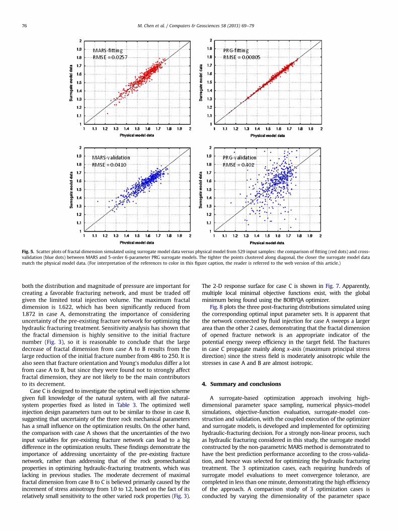
To illustrate the surrogate model quality regarding fitting andvalidation, the scatter plots of fractal dimension simulated bysurrogate models versus GEOS-2D from 529 sample inputs arecompared between MARS model and the best-fitted, but worst-validated PRG model (5-order 6-parameter) (Fig. 5). The closer thepoints are to the diagonal line, the better the surrogate modelmatches the physical model. It is seen that the points are clusteredclosely along the diagonal line for the PRG model fitting(RMSE¼0.00805), but are significantly scattered for cross-validation (RMSE¼0.401). Conversely, points in both the MARS

Table 2Evaluation of surrogate models for fracture network at final time.

Construction method Estimated Coefficients RMSE

Fitting Validation

MARS – 0.0257 0.0410GSP – 0.0278 0.04281-order 7-parameter PRG 7 0.0473 0.04832-order 6-parameter PRG 27 0.0390 0.04582-order 7-parameter PRG 35 0.0378 0.04363-order 5-parameter PRG 55 0.0326 0.04523-order 6-parameter PRG 83 0.0300 0.04583-order 7-parameter PRG 119 0.0283 0.04624-order 5-parameter PRG 125 0.0258 0.05064-order 6-parameter PRG 209 0.0221 0.05895-order 5-parameter PRG 251 0.0184 0.05684-order 7-parameter PRG 329 0.0169 0.08655-order 6-parameter PRG 461 0.00805 0.4010

Mean: 1.58

Std: 0.112

Fig. 4. Statistics of 529 derived fractal dimension: (a) mean for 9 injection time orvolumes and (b) PDF and CDF at finial time (51.1 s or 12.8 m3 injected fluid volume).

M. Chen et al. / Computers & Geosciences 58 (2013) 69–79 75

fitting and cross-validation scatter plots are moderately spread with0.0257 and 0.0410 of RMSE, respectively.

3.5. Horizontal well design optimization

The problem of interest is to find the favorable fracture-stimulation well design variables, namely, well center y location

and the perforation length, in the presence of natural-systemuncertainty. To investigate how natural-system uncertainty affectsoptimal well design, three optimization cases with sequentiallydecreasing natural-system uncertainty are performed for the lastsnapshot at an injection time of 51.1 s. Case A searches theminimum objective function (maximum fractal dimension) in a7-D parameter space, with two design variables and with fivenatural-system variables treated as uncertain. Case B is adaptedfrom case A, with the uncertainty reduced by fixing the fractureorientation and number, which are two parameters describing thepre-existing fracture network. In case C, only well location andlength are allowed to vary within the specified ranges during theoptimization process, by further fixing the three geomechanicalvariables affecting fracture propagation, minimal principal stress,stress anisotropy, and Young’s modulus. The objective function tobe minimized is the negative fractal dimension. All the threeoptimization cases are efficiently conducted using surrogate mod-els without rerunning the expensive physics-based GEOS-2D, dueto the flexibility of our surrogate-based approach. The BOBYQAoptimizer, coupled with the selected MARS models, is executed forthe three inverse problems.

Fig. 6 depicts the optimization processes, which involvessearching the minimal objective function for each of the threecases. It is seen that the number of evaluations of the surrogatemodel required to satisfy the convergence criteria (10−6) is 337,269 and 994, respectively. Each of the optimizations requireshundreds of model evaluations and can be completed in less thana minute, while a single realization conducted with the GEOS-2Dcode costs tens of hours. Moreover, a physics-based model isusually not as smooth as its surrogate, implying that a greaternumber of model evaluations are required for convergence thanrequired by surrogate-based optimization. As a result, the high-efficient surrogate-based optimization approach can make theotherwise computationally prohibitive procedure practicallyachievable. An example of an expensive procedure is Bayesianstochastic joint inversion modeling using hard (borehole core) andsoft data (geophysical survey), which usually entails expensiveMarkov Chain Monte Carlo sampling. Another advantage of thesurrogate-based approach is its high degree of flexibility. Once thetraining data is generated from the expensive physics-modelsimulations, numerous surrogate models can be constructed andvalidated for optimization within a very short time.

The optimal values of the parameter sets corresponding to theminimum objectives are listed in Table 3. Case A represents ascenario in which the hydraulic fracturing treatment is designedwith minimal knowledge of the targeted field; thus, a wide rangeof the natural-system properties must be accounted for. Theoptimal location of the well center is found to be 4.31 m on they-axis, and the optimal well length is 0.08 m. This indicates that, toobtain a maximum fractal dimension, the fluid should be injectedin just one injection node at y¼4 m, and at the rate of 0.25 m3/s,if fracturing is to be optimized for this level of natural-systemuncertainty. With the entire injection rate concentrated at onenode, the maximum possible hydraulic pressure is achieved,which confirms our intuition about what will maximize thegrowth of the fracture network.

Case B assumes that both the fracture orientation and fracturenumber of the pre-existing network are already determined to be11 and 2501, respectively, on the basis of borehole core data orother geophysical measurements. The optimal well design para-meters (position and length) are found to be 5.09 m and 21.3 m,which corresponds to a hydraulic fracturing scheme where fluid isinjected into 11 nodes, centered at y¼5 m, with each injected at arate of 0.25/11¼0.0227 m3/s. Unlike case A, where all of the fluidinjection (and pressurization) is concentrated in one node, pres-surization in case B is distributed along 11 nodes, suggesting that

Fig. 5. Scatter plots of fractal dimension simulated using surrogate model data versus physical model from 529 input samples: the comparison of fitting (red dots) and cross-validation (blue dots) between MARS and 5-order 6-parameter PRG surrogate models. The tighter the points clustered along diagonal, the closer the surrogate model datamatch the physical model data. (For interpretation of the references to color in this figure caption, the reader is referred to the web version of this article.)

M. Chen et al. / Computers & Geosciences 58 (2013) 69–7976

both the distribution and magnitude of pressure are important forcreating a favorable fracturing network, and must be traded offgiven the limited total injection volume. The maximum fractaldimension is 1.622, which has been significantly reduced from1.872 in case A, demonstrating the importance of consideringuncertainty of the pre-existing fracture network for optimizing thehydraulic fracturing treatment. Sensitivity analysis has shown thatthe fractal dimension is highly sensitive to the initial fracturenumber (Fig. 3), so it is reasonable to conclude that the largedecrease of fractal dimension from case A to B results from thelarge reduction of the initial fracture number from 486 to 250. It isalso seen that fracture orientation and Young’s modulus differ a lotfrom case A to B, but since they were found not to strongly affectfractal dimension, they are not likely to be the main contributorsto its decrement.

Case C is designed to investigate the optimal well injection schemegiven full knowledge of the natural system, with all five natural-system properties fixed as listed in Table 3. The optimized wellinjection design parameters turn out to be similar to those in case B,suggesting that uncertainty of the three rock mechanical parametershas a small influence on the optimization results. On the other hand,the comparison with case A shows that the uncertainties of the twoinput variables for pre-existing fracture network can lead to a bigdifference in the optimization results. These findings demonstrate theimportance of addressing uncertainty of the pre-existing fracturenetwork, rather than addressing that of the rock geomechanicalproperties in optimizing hydraulic-fracturing treatments, which waslacking in previous studies. The moderate decrement of maximalfractal dimension from case B to C is believed primarily caused by theincrement of stress anisotropy from 1.0 to 1.2, based on the fact of itsrelatively small sensitivity to the other varied rock properties (Fig. 3).

The 2-D response surface for case C is shown in Fig. 7. Apparently,multiple local minimal objective functions exist, with the globalminimum being found using the BOBYQA optimizer.

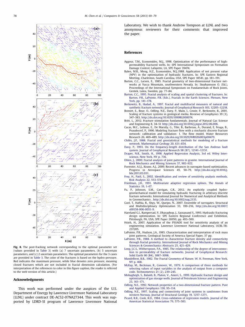
Fig. 8 plots the three post-fracturing distributions simulated usingthe corresponding optimal input parameter sets. It is apparent thatthe network connected by fluid injection for case A sweeps a largerarea than the other 2 cases, demonstrating that the fractal dimensionof opened fracture network is an appropriate indicator of thepotential energy sweep efficiency in the target field. The fracturesin case C propagate mainly along x-axis (maximum principal stressdirection) since the stress field is moderately anisotropic while thestresses in case A and B are almost isotropic.

4. Summary and conclusions

A surrogate-based optimization approach involving high-dimensional parameter space sampling, numerical physics-modelsimulations, objective-function evaluation, surrogate-model con-struction and validation, with the coupled execution of the optimizerand surrogate models, is developed and implemented for optimizinghydraulic-fracturing decision. For a strongly non-linear process, suchas hydraulic fracturing considered in this study, the surrogate modelconstructed by the non-parametric MARS method is demonstrated tohave the best prediction performance according to the cross-valida-tion, and hence was selected for optimizing the hydraulic fracturingtreatment. The 3 optimization cases, each requiring hundreds ofsurrogate model evaluations to meet convergence tolerance, arecompleted in less than oneminute, demonstrating the high efficiencyof the approach. A comparison study of 3 optimization cases isconducted by varying the dimensionality of the parameter space

M. Chen et al. / Computers & Geosciences 58 (2013) 69–79 77

without rerunning expensive physics-model simulations. Moreover,additional optimizations using surrogate models can be performedquickly and easily for particular purposes if necessary, for example,reducing the uncertainty of an input variable by narrowing its range.

The comparison study shows the optimization results whichdepend on the degree of uncertainty of the pre-existing fracturenetworks. This indicates the importance of incorporating informationabout pre-existing fracture networks into the process of optimizinghydraulic fracturing treatment, which has been largely overlooked byprevious optimization studies in the literature. In contrast, theinfluence of uncertainty in rock geomechanical properties on the

Table 3Optimization of well center location and length for fracture network at final time.

Input sample space Case A: 7-D

Range Opt.

Fracture orientation 0–135 121Initial fracture number 50–500 486Minimum principal stress sh (MPa) 10–15 13.02Stress anisotropy (sH/sh) 1.0–1.5 1.07Young’s modulus (GPa) 5–50 38.33Injection well center on y-axis (m) −20 to 20 4.31Injection well length (m) 0–40 0.08Maximum fractal dimension 1.872

Fig. 6. Minimal objective searching curve for optimization case with (a) 7 uncertainparameters, (b) 5 uncertain parameters, and (c) 2 uncertain parameters. Theoptimal parameter values for the 3 cases are proved in Table 3.

optimal injection scheme is found to be less important. These findingssuggest that the pre-existing fracture network, rather than thegeomechanical properties, should be the top priority to be character-ized before designing a hydraulic fracturing treatment.

The statistical analysis of the training data and fracture net-works for the three optimized hydraulic-fracturing cases indicatesthat fractal dimension is a useful metric for quantifying the densityand connectivity of a fracture network. Furthermore, the scale-invariant nature of the fractal makes it a universal indicator for thefracture network across wide range of spatial scales, from corethrough outcrop to aerial image scale. The successful incorporationof fractal dimension into the efficient surrogate-based approach inthis study provides a useful solution for other inverse problemsthat suffer from the heavy computational burden and multi-scalemeasurements, such as the stochastic joint inversion problem.

The decreasing growth rate of the mean fractal dimension withinjection time implies the diminishing value of continuing thehydraulic fracturing operation. Therefore, there exists a cost-efficient time to stop the fracturing operation, that is, the injectiontime and the rate need to be optimized for economic objective.Although this paper is focused on incorporating uncertainty of thenatural system into optimization and hence only considers thephysical criterion as the objective function, the presentedsurrogate-based optimization approach, can be modified to findoptimal injection rate and time by integrating an energy produc-tion model and economic model to derive both physical andeconomic criteria as the objective function.

Case B: 5-D Case C: 2-D

Range Opt. Range Opt.

1 – 1 –

250 – 250 –

10–15 13.27 12.5 –

1.0–1.5 1.00 1.2 –

5–50 48.65 25 –

−20 to 20 5.09 −20 to 20 5.090–40 21.3 0–40 21.9

1.622 1.547

Fig. 7. The visualized response surface with 2 uncertain design parameters, i.e.,horizontal well center at y-axis and well length.

Fig. 8. The post-fracking network corresponding to the optimal parameter set(values provided in Table 3) with (a) 7 uncertain parameters, (b) 5 uncertainparameters, and (c) 2 uncertain parameters. The optimal parameters for the 3 casesare provided in Table 3. The color of the fractures is based on the hydro-pressure.Red indicates the maximum pressure, while blue denotes zero pressure, meaningclosed fractures which are not included in fractal dimension calculation. (Forinterpretation of the references to color in this figure caption, the reader is referredto the web version of this article.)

M. Chen et al. / Computers & Geosciences 58 (2013) 69–7978

Acknowledgments

This work was performed under the auspices of the U.S.Department of Energy by Lawrence Livermore National Laboratory(LLNL) under contract DE-AC52-07NA27344. This work was sup-ported by LDRD-SI program of Lawrence Livermore National

Laboratory. We wish to thank Andrew Tompson at LLNL and twoanonymous reviewers for their comments that improvedthe paper.

References

Aggour, T.M., Economides, M.J., 1998. Optimization of the performance of high-permeability fractured wells. In: SPE International Symposium on FormationDamage Control, Lafayette, LA, SPE Paper 39474.

Balen, M.R., Meng, H.Z., Economides, M.J.,1988. Application of net present value(NPV) in the optimization of hydraulic fractures. In: SPE Eastern RegionalMeeting, Charleston, South Carolina, USA, SPE Paper 18541, pp. 181–191.

Barton, C.C., Larsen, E., 1985. Fractal geometry of two-dimensional fracture net-works at Yucca Mountain, southwestern Nevada. In: Stephannson O. (Ed.),Proceedings of the International Symposium on Fundamentals of Rock Joints,Gentek, Lulea, Sweden, pp. 77–84.

Barton, C.C., 1995. Fractal analysis of scaling and spatial clustering of fractures. In:Barton, P.R., LaPointe, P.R. (Eds.), Fractals in the Earth Sciences. Plenum, NewYork, pp. 141–178.

Berkowitz, B., Hadad, A., 1997. Fractal and multifractal measures of natural andsynthetic fracture networks. Journal of Geophysical Research 103, 12205–12218.

Bonnet, E., Bour, O., Odling, N.E., Davy, P., Main, I., Cowie, P., Berkowitz, B., 2001.Scaling of fracture systems in geological media. Reviews of Geophysics 39 (3),347–383, http://dx.doi.org/10.1029/1999RG000074.

Britt, L., 2012. Fracture stimulation fundamentals. Journal of Natural Gas Scienceand Engineering 8, 34–51 http://dx.doi.org/10.1016/j.jngse.2012.06.006.

Cacas, M.C., Ledoux, E., De Marsily, G., Tilie, B., Barbreau, A., Durand, E, Feuga, B.,Peaudecerf, P., 1990. Modeling fracture flow with a stochastic discrete fracturenetwork: calibration and validation: 1. The flow model. Water ResourcesResearch 26, 469–489, http://dx.doi.org/10.1029/WR026i003p00479.

Chilès, J.P., 1988. Fractal and geostatistical methods for modeling of a fracturenetwork. Mathematical Geology 20, 631–654.

Davy, P., 1993. On the frequency-length distribution of the San Andreas faultsystem. Journal of Geophysical Research 98 (B7), 12141–12151.

Draper, N.R., Smith, H., 1998. Applied Regression Analysis, 3rd ed. Wiley Inter-science, New York, NY p. 736.

Ehlen, J., 2000. Fractal analysis of joint patterns in granite. International Journal ofRock Mechanics and Mining Sciences 37, 902–922.

Forrester, A.I.J., Keane, A.J., 2009. Recent advances in surrogate-based optimization.Progress in Aerospace Sciences 45, 50–79, http://dx.doi.org/10.1016/j.bbr.2011.03.031.

Frey, H., Patil, S., 2002. Identification and review of sensitivity analysis methods.Risk Analysis 22, 553–578.

Friedman, J.H., 1991. Multivariate adaptive regression splines. The Annals ofStatistics 19, 1–67.

Fu, P., Johnson, S.M., Carrigan, C.R., 2012. An explicitly coupled hydro-geomechanical model for simulating hydraulic fracturing in arbitrary discretefracture networks. International Journal for Numerical and Analytical Methodsin Geomechanics , http://dx.doi.org/10.1002/nag.2135.

Goel, T., Haftka, R., Shyy, W., Queipo, N., 2007. Ensemble of surrogates. Structuraland Multidisciplinary Optimization 33, 199–216, http://dx.doi.org/10.1007/s00158-006-0051-9.

Hareland G.l., Rampersad, P., Dharaphop, J., Sasnanand S., 1993. Hydraulic fracturingdesign optimization. In: SPE Eastern Regional Conference and Exhibition,Pittsburgh, PA, USA, SPE Paper 26950, pp. 493–500.

Hsieh, H., 2007. Application of the PSUADE tool for sensitivity analysis of anengineering simulation. Lawrence Livermore National Laboratory, UCRL-TR-237205.

LaPointe, P.R., Hudson, J.A., 1985. Characterization and interpretation of rock massjoint patterns. Geological Society of America Special Paper, 37 pp.

LaPointe, P.R., 1988. A method to characterize fracture density and connectivitythrough fractal geometry. International Journal of Rock Mechanics and MiningSciences & Geomechanics Abstracts 25, 421–429.

Long, J.C.S., Witherspoon, P.A., 1985. The relationship of the degree of interconnec-tion to permeability of fracture networks. Journal of Geophysical Research:Solid Earth 90 (B4), 3087–3098.

Mandelbrot, B.B., 1982. The Fractal Geometry of Nature. W. H. Freeman, New York,NY p. 468.

McKay, M., Beckman, R., Conover, W., 1979. A comparison of three methods forselecting values of input variables in the analysis of output from a computercode. Technometrics 21 (2), 239–245.

Mohaghegh, S., Balanb, B., Platon, V., Ameri, S., 1999. Hydraulic fracture design andoptimization of gas storage wells. Journal of Petroleum Science and Engineering23, 161–171.

Odling, N.E., 1992. Network properties of a two-dimensional fracture pattern. Pureand Applied Geophysics 138, 95–114.

Odling, N.E., 1997. Scaling and connectivity of joint systems in sandstones fromwestern Norway. Journal of Structural Geology 19, 1257–1271.

Picard, R.R., Cook, R.D., 1984. Cross-validation of regression models. Journal of theAmerican Statistical Association 79, 575–583.

M. Chen et al. / Computers & Geosciences 58 (2013) 69–79 79

Powell, M.J.D., 2009. The BOBYQA algorithm for bound constrained optimizationwithout derivatives. Report DAMTP 2009/NA06, Centre for MathematicalSciences, University of Cambridge, UK.

Queipo, N.V., Verde, A.J., Canelon, J., Pintos, S., 2002. Efficient global optimizationfor hydraulic fracturing treatment design. Journal of Petroleum Science andEngineering 35, 151–166.

Queipo, N.V., Haftka, R.T., Shyy, W., Geol, T., Vaidyanathan, R., Tucker, P.K., 2005.Surrogate-based analysis and optimization. Progress in Aerospace Sciences 41,1–28, http://dx.doi.org/10.1016/j.paerosci.2005.02.001.

Ralph, W., VeatchJr.W., 1986. Economics of fracturing: some methods, examples andcase studies. In: SPE 61th Annual Technical Conference and Exhibition, NewOrleans, Atlanta, USA, SPE Paper 15509, pp. 1–16.

Renshaw, C.E., 1999. Connectivity of joint networks with power law lengthdistributions. Water Resources Research 35 (9), 2661–2670.

Reeves, D.M., Benson, D.A., Meerschaert, M.M., 2008. Transport of conservativesolutes in simulated fracture networks: 1. Synthetic data generation. WaterResources Research 44, http://dx.doi.org/10.1029/2007WR006069.

Rueda, J.I., Rahim, Z., Holditch, S.A., 1994. Using a mixed integer linear programmingtechnique to optimize a fracture treatment design. In: SPE Eastern RegionalMeeting, Charleston, South Carolina, USA, SPE Paper 29184, pp. 233–244.

Sanchez, E., Pintos, S., Queipo, N., 2008. Toward and optimal ensemble of kernel-basedapproximations with engineering applications. Structural and MultidisciplinaryOptimization 36, 247–261, http://dx.doi.org/10.1007/s00158-007-0159-6.

Sobol’, I, 1993. Sensitivity estimates for non-linear mathematical models. Mathe-matical Modeling and Computational Experiment 4, 407–414.

Sun, Y., Tong, C., Duan, Q., Buscheck, T.A., Blink, J.A., 2012. Combining simulation andemulation for calibrating sequentially reactive transport systems. Transport inPorous Media 92 (2), 509–526, http://dx.doi.org/10.1007/s11242-011-99170-4.

Tong, C., 2009. PSUADE user’s manual (Version 1.2.0). Lawrence Livermore NationalLaboratory, LLNL-SM-407882.

Walsh, J., Watterson, J.J., 1993. Fractal analysis of fracture pattern using thestandard box-counting technique: valid and invalid methodologies. Journal ofStructural Geology 15, 1509–1512.

Wang, G.G., Shan, S., 2007. Review of metamodeling techniques in support ofengineering design optimization. Journal of Mechanical Design 129 (4), 370–-380, http://dx.doi.org/10.1115/1.2429697.

Wemhoff, A.P., Hsieh, H., 2007. TNT Prout-Tompkins kinetics calibration withPSUADE. Lawrence Livermore National Laboratory, UCRL-TR-230194.

Williams, C.K.I., Rasmussen, C.E., 1996. Gaussian process for regression. In: Touretzky,D.S., Mozer, M.C., Hasselmo, M.E. (Eds.), Advances in Neural Information Proces-sing Systems, 8. MIT Press, Cambridge, pp. 514–520.