i Modeling and Simulation of Electromagnetic Damper to Improve Performance of a Vehicle during Cornering by Saad Bin Abul Kashem A Thesis Submitted to the Swinburne University of Technology In Fulfillment of the Requirements for the Degree of PhD in the Faculty of Engineering and Industrial Sciences Saad Bin Abul Kashem, 2013 Swinburne University of Technology Hawthorn, Melbourne, VIC 3122
Transcript
i
Modeling and Simulation of
Electromagnetic Damper to
Improve Performance of a Vehicle
during Cornering
by
Saad Bin Abul Kashem
A Thesis Submitted to the Swinburne University of Technology In Fulfillment of the
Requirements for the Degree of PhD
in the Faculty of Engineering and Industrial Sciences
Saad Bin Abul Kashem, 2013 Swinburne University of Technology
Hawthorn, Melbourne, VIC 3122
ii
Author's declaration
This is to certify that the thesis submitted to the Swinburne University of
Technology for the award of the degree of Doctor of Philosophy. The contents of
this thesis, in full or in parts, have not been submitted to any other Institute or
University for the award of any degree or diploma. I hereby declare that I am the
sole author of this thesis. To the best of my knowledge, the thesis contains no
material previously published or written by another person except where due
reference is made in the text.
Saad Bin Abul Kashem
iii
Abstract
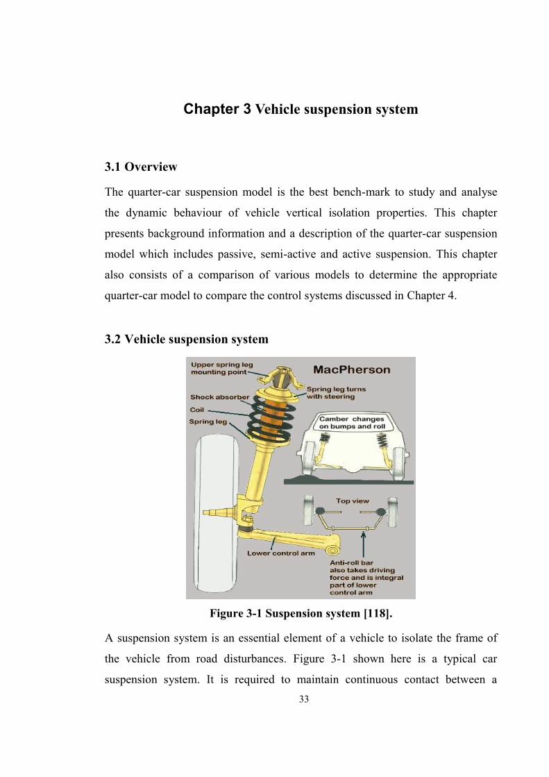
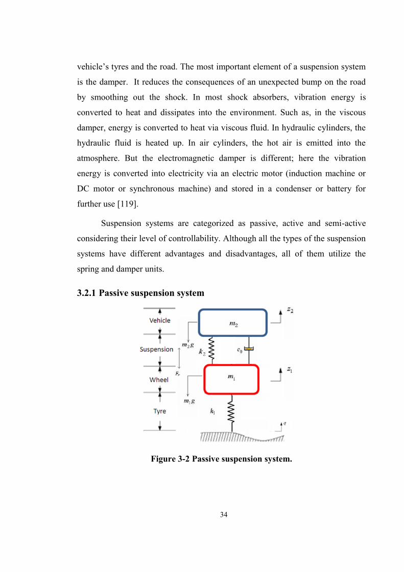
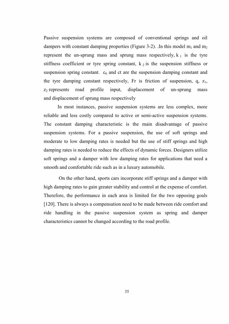
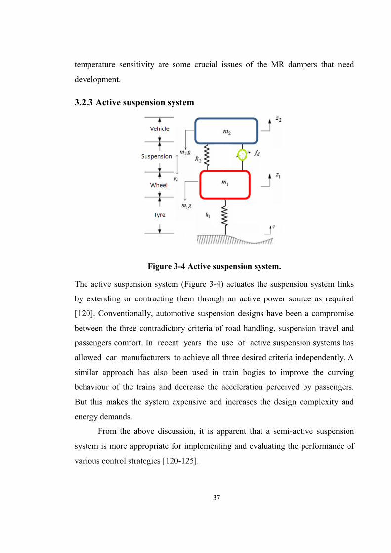
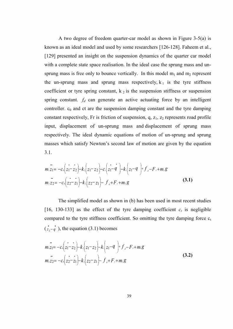
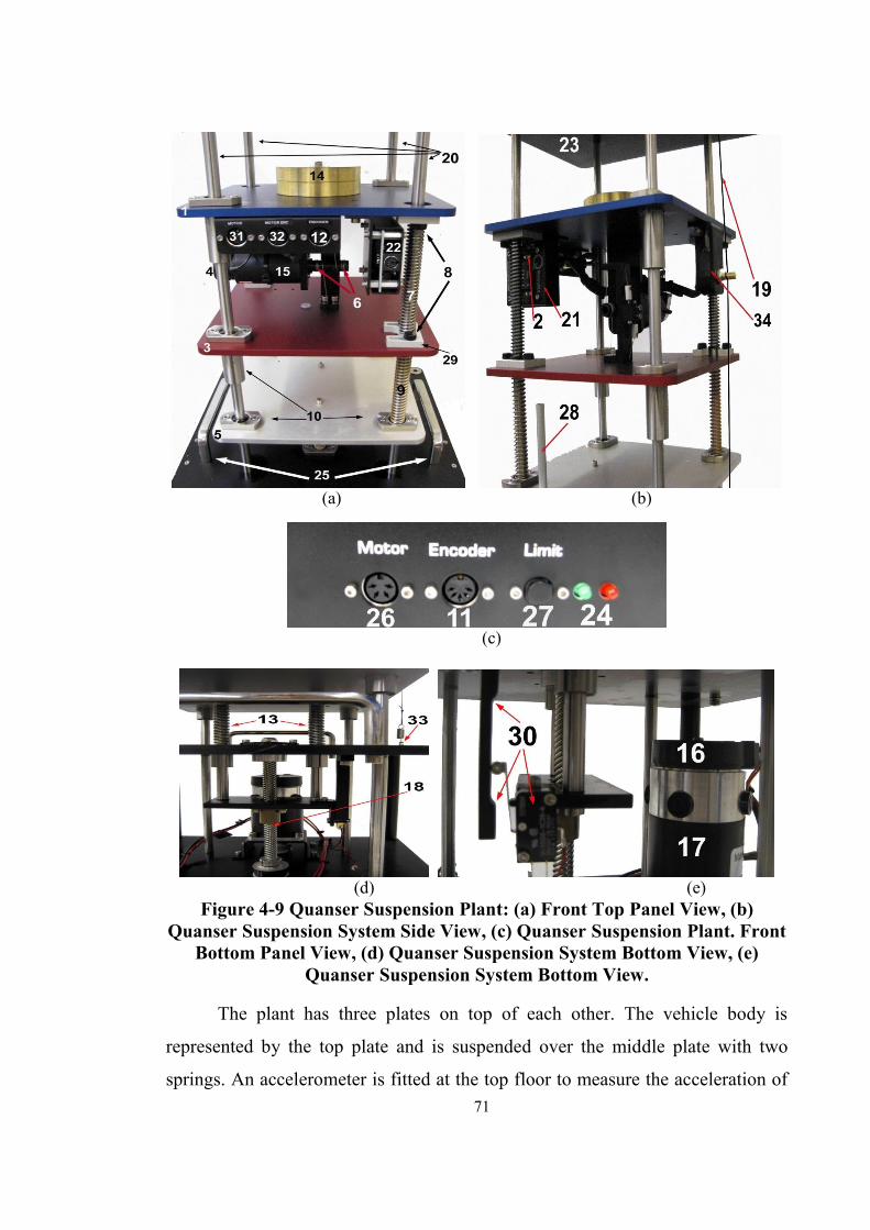
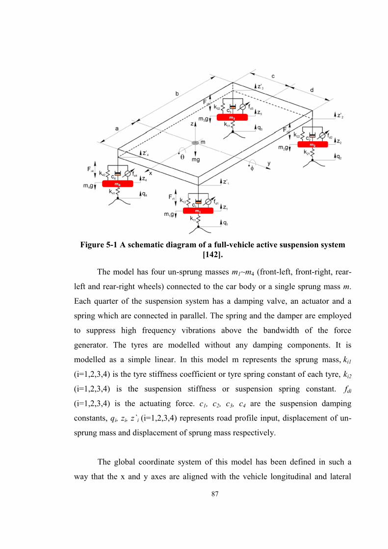
A suspension system is an essential element of a vehicle to isolate the frame of
the vehicle from road disturbances. It is required to maintain continuous contact
between a vehicle’s tyres and the road. In order to achieve the desired ride
comfort, road handling performance, many researches has been conducted. A
new modified skyhook control strategy with adaptive gain that dictates the
vehicle’s semi-active suspension system is presented. The proposed closed loop
feedback system first captures the road profile input over a certain period. Then it
calculates the best possible value of the skyhook gain for the subsequent process.
Meanwhile the system is controlled according to the new modified skyhook
control law using an initial or previous value of the skyhook gain. In this
research, the proposed suspension system is compared with passive and three
other recently reported skyhook controlled semi-active suspension systems
through a virtual environment with MatLab/SIMULINK as well as an
experimental analysis with Quanser suspension plant. Its performances have been
evaluated in terms of ride comfort and road handling performance. The model
has been validated in accordance to the international standards of admissible
acceleration levels ISO2631 and human vibration perception. This control
strategy has also been employed on the full car model to improve the isolation of
the vibration and handling performance of the road vehicle.
This thesis also describes the development of a new analytical full vehicle
model with nine degrees of freedom, which uses the new modified skyhook
strategy to control the full vehicle vibration problem. Nowadays, many
researchers are working on active tilting technology to improve vehicle
cornering. But in those work, the effect of road bank angle is not considered in
the control system design or in the dynamic model of the tilting standard
passenger vehicles. The non-incorporation of road bank angle creates a non-zero
steady state torque requirement. Therefore, in this research this phenomenon was
iv
addressed while designing the direct tilt control and the dynamic model of the
full car model.
This research has indicated the potential of the SKDT suspension system
in improving cornering performances of the vehicle and paves the way for future
work on vehicle’s integrated system for chassis control.
Appendix A ......................................................................................................... 248
Appendix B ......................................................................................................... 250
Appendix C ......................................................................................................... 255
xi
List of Figures Figure 1-1 Vehicle suspension system..............................................................................2 Figure 1-2 Rear suspension system without wheel of a vehicle.......................................2 Figure 1-3 The Passive, Semi-active and Active suspension system. ................................ 3
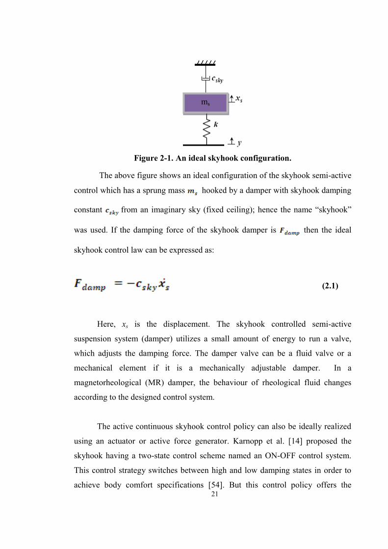
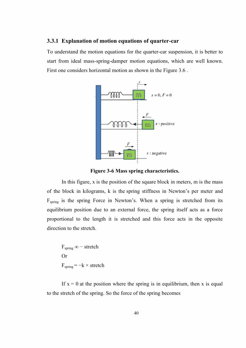
Figure 2-1. An ideal skyhook configuration. ................................................................... 21
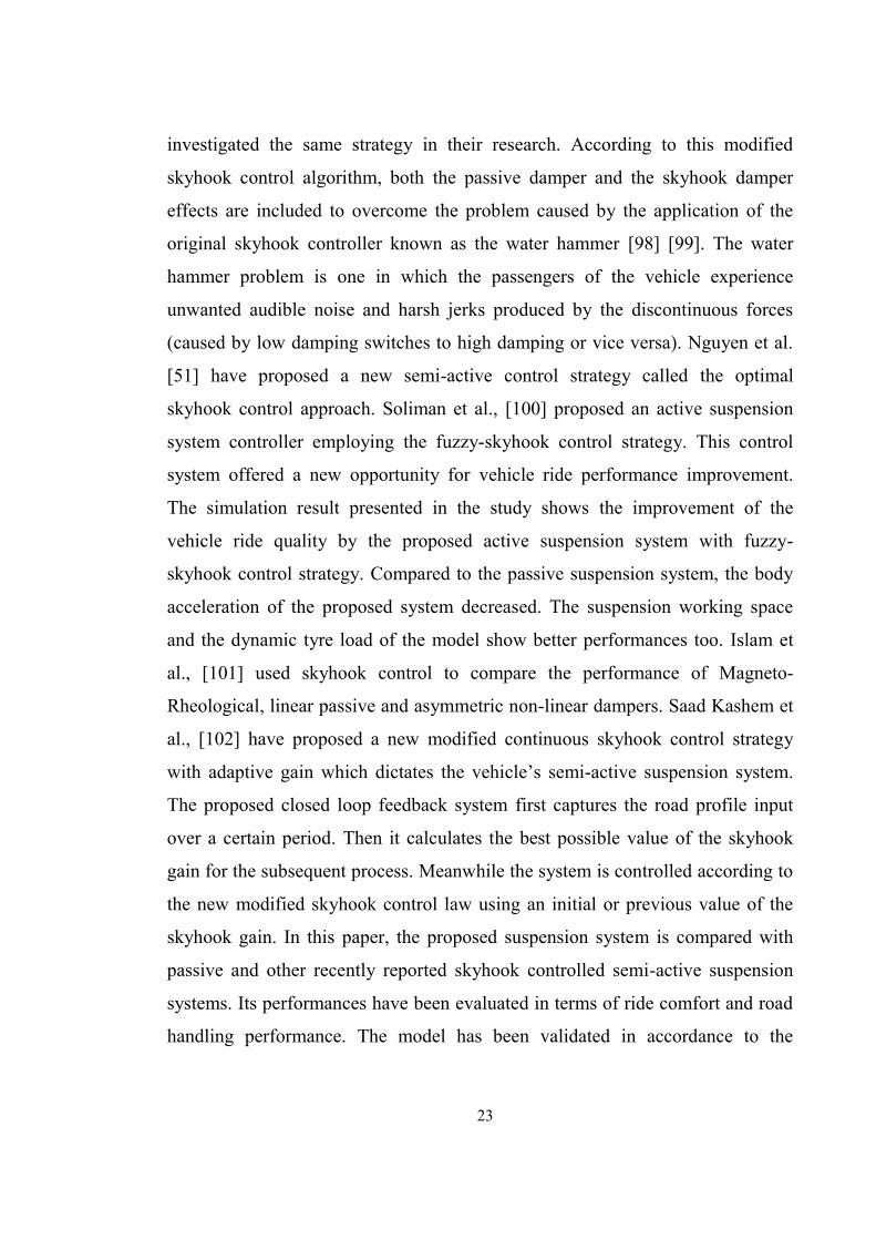
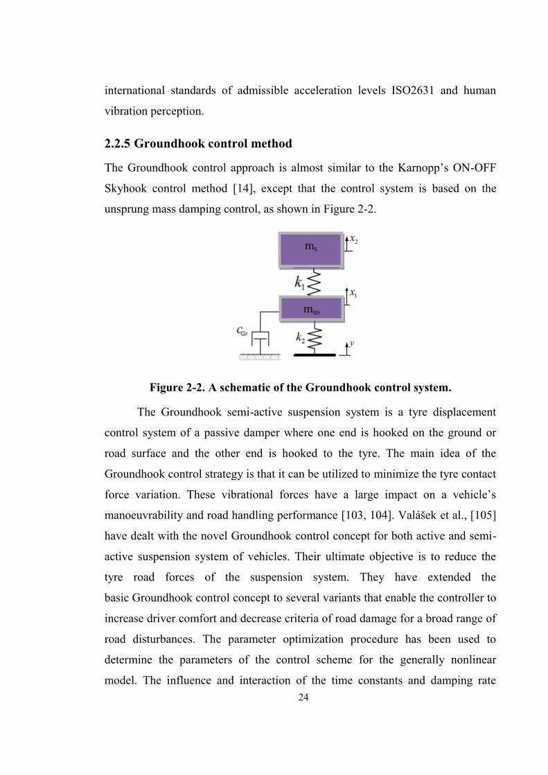
Figure 2-2. A schematic of the Groundhook control system. ......................................... 24
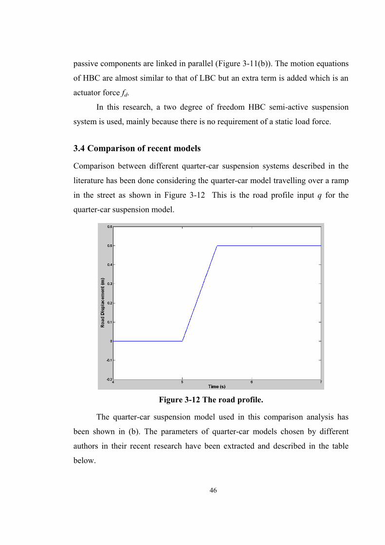
Figure 3-12 The road profile. .......................................................................................... 46
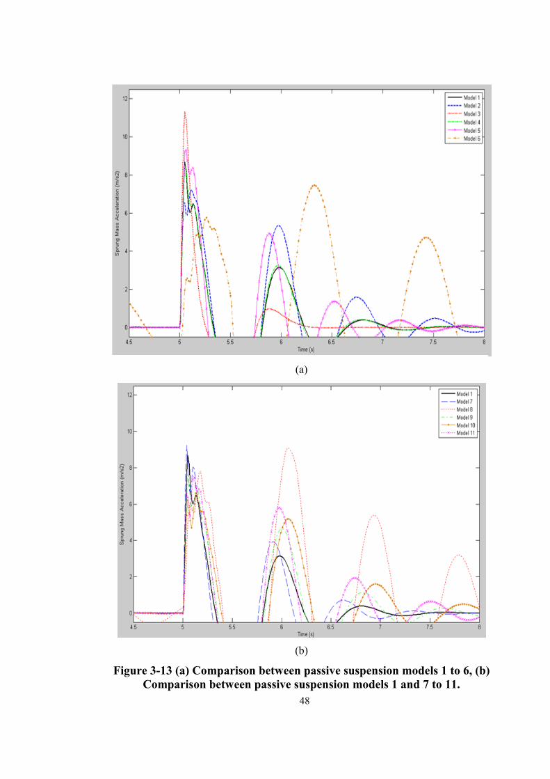
Figure 3-13 (a) Comparison between passive suspension models 1 to 6, (b) Comparison between passive suspension models 1 and 7 to 11. ....................................................... 48
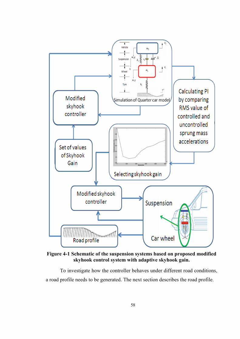
Figure 4-1 Schematic of the suspension systems based on proposed modified skyhook control system with adaptive skyhook gain....................................................................58 Figure 4-2 (a) The time histories of three classes of roads, (b) Power spectral density of three classes of road. ...................................................................................................... 61
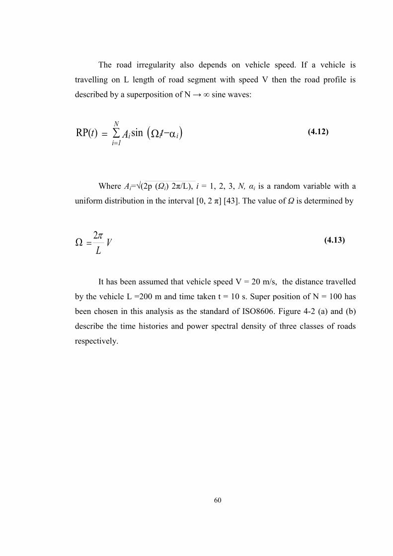
Figure 4-3 The time history of road profile. .................................................................... 63
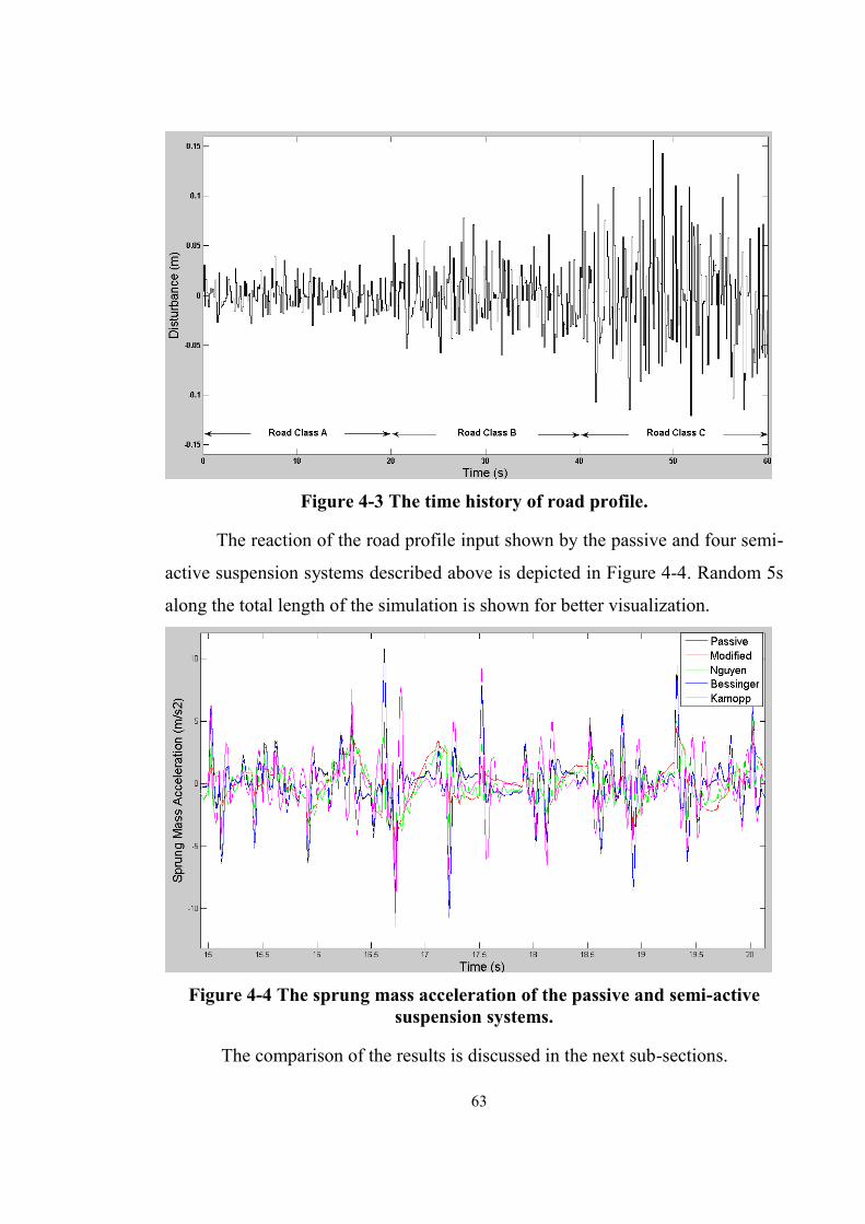
Figure 4-4 The sprung mass acceleration of the passive and semi-active suspension systems. ........................................................................................................................... 63
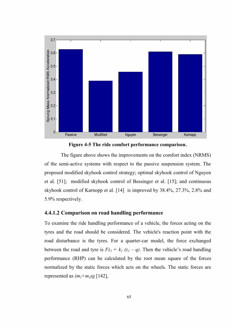
Figure 4-5 The ride comfort performance comparison. ................................................. 65
Figure 4-6 The road handling performance comparison. ............................................... 66
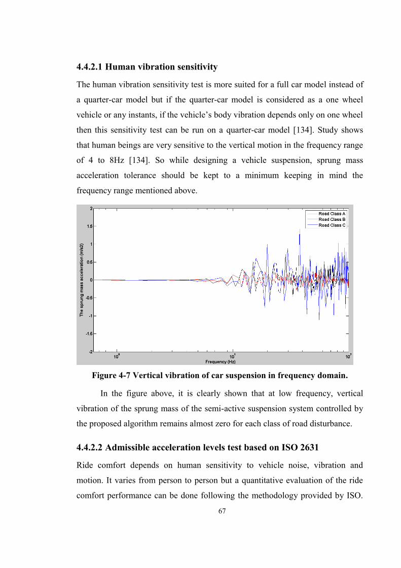
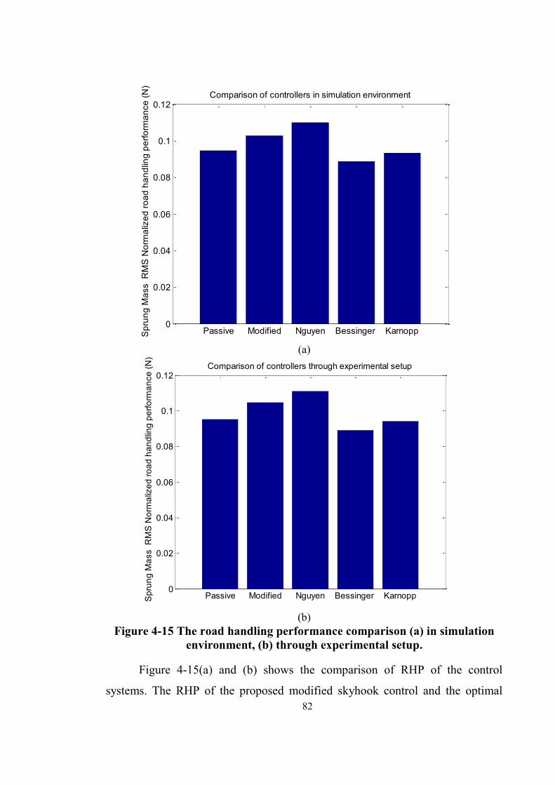
Figure 4-7 Vertical vibration of car suspension in frequency domain. ........................... 67
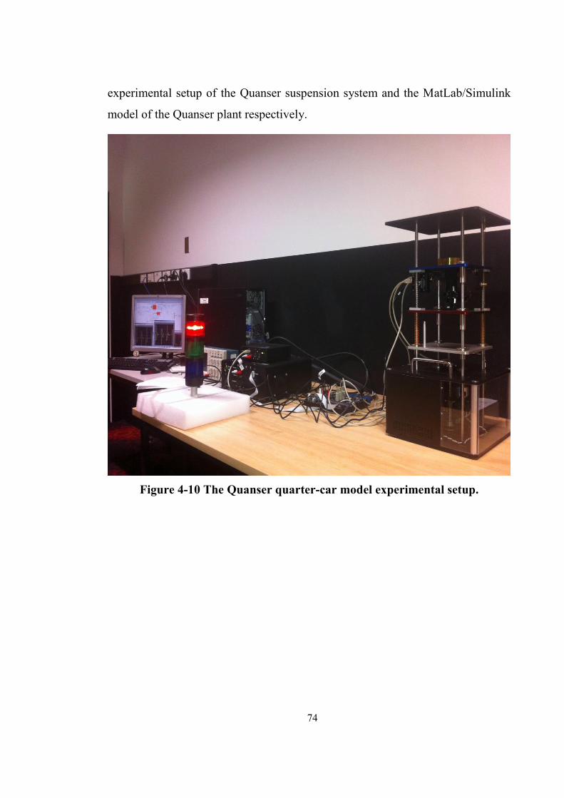
Figure 4-9 Vehicle suspension system............................................................................71 Figure 4-10 The Quanser quarter-car model experimental setup. ................................. 74
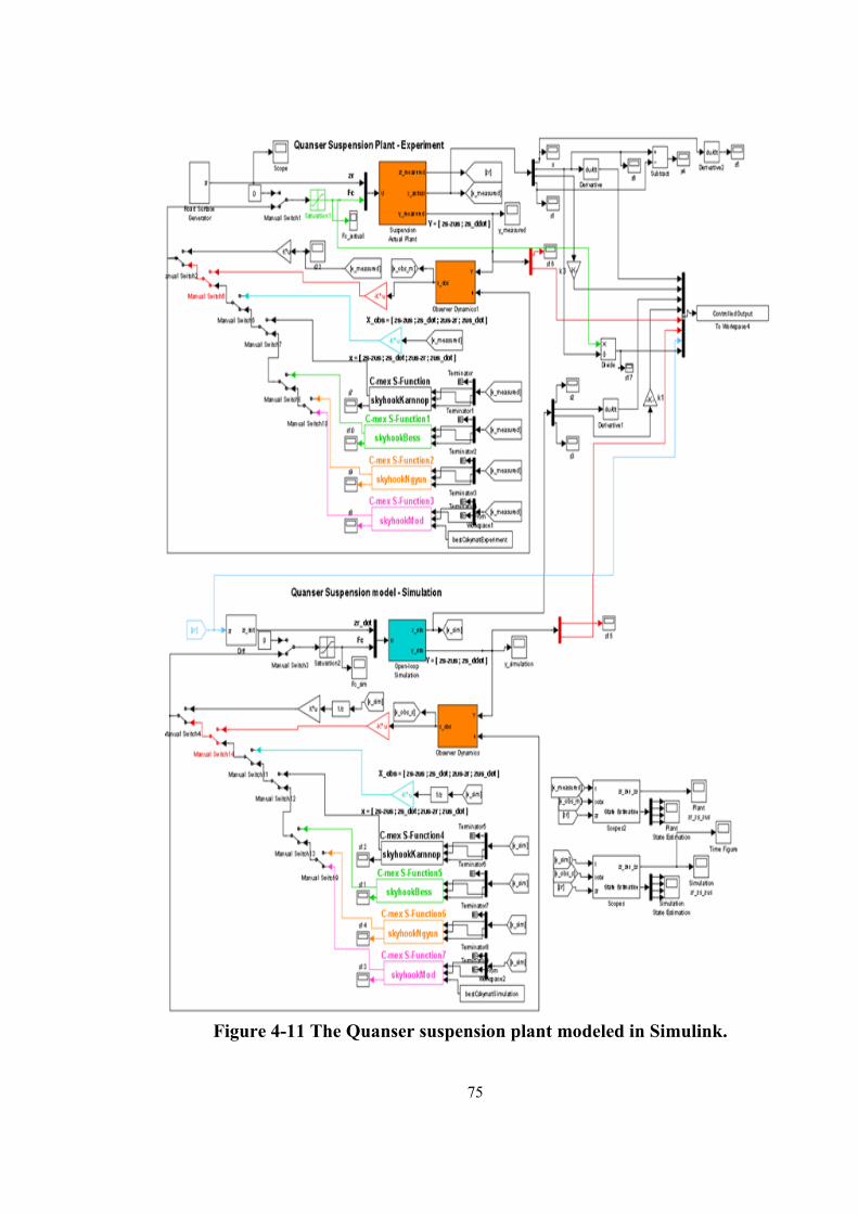
Figure 4-11 The Quanser suspension plant modeled in Simulink................................... 75
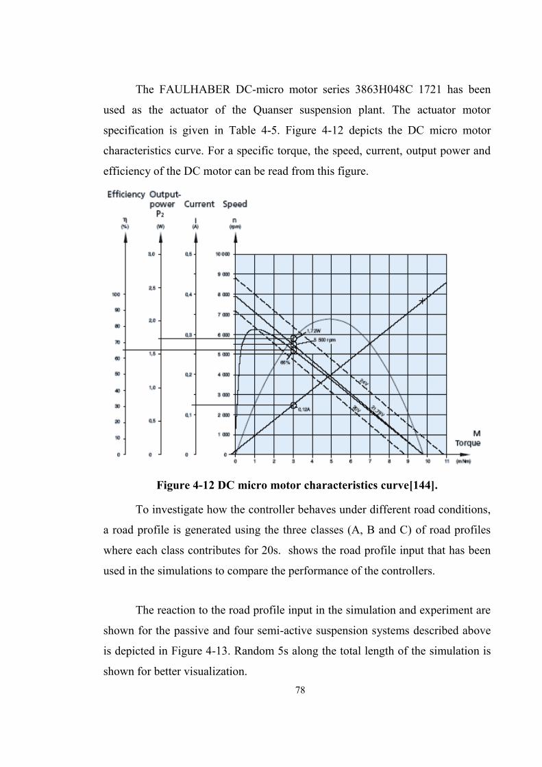
Figure 4-12 DC micro motor characteristics curve[144]. ................................................ 78
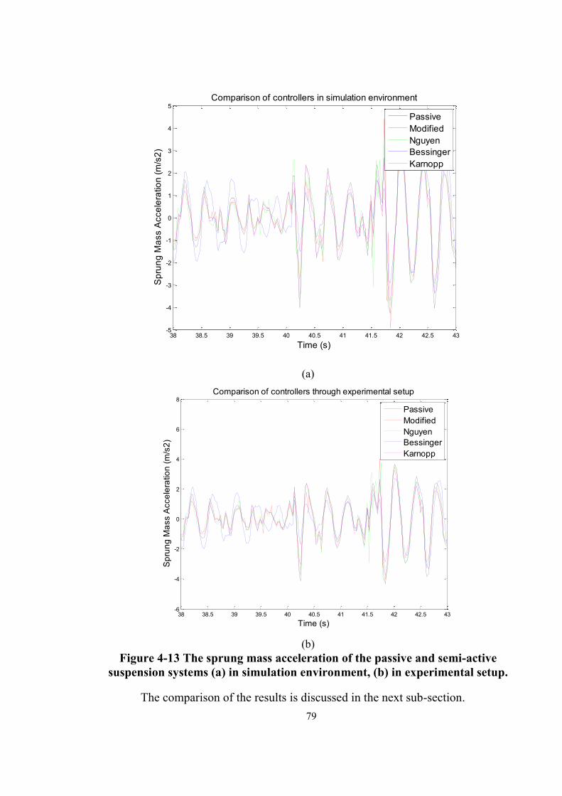
Figure 4-13 The sprung mass acceleration of the passive and semi-active suspension systems (a) in simulation environment, (b) in experimental setup. ............................... 79
Figure 4-14 The ride comfort performance comparison (a) in simulation environment, (b) through experimental setup. ..................................................................................... 81
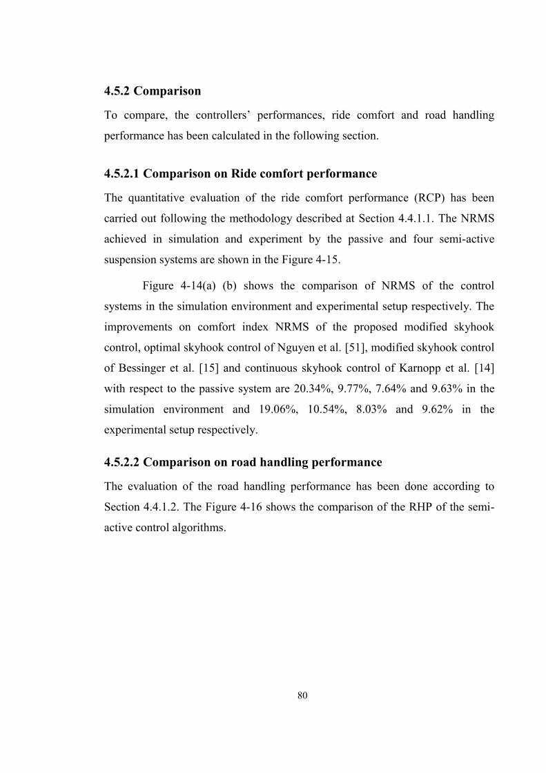
Figure 4-15 The road handling performance comparison (a) in simulation environment, (b) through experimental setup. .................................................................................... .82
xii
Figure 4-16 Vertical vibration of car suspension in frequency domain. ......................... 83
Figure 5-1 A schematic diagram of a full-vehicle active suspension system [142]......... 87
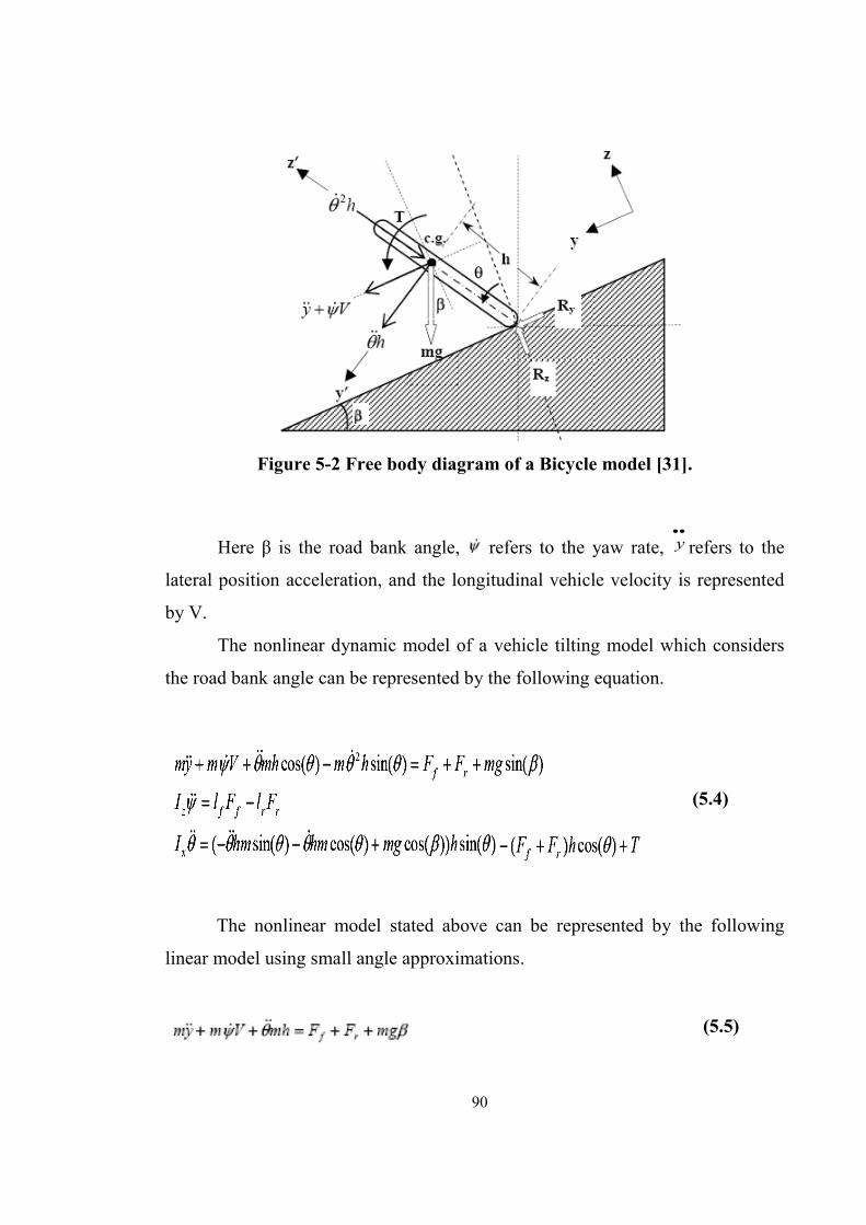
Figure 5-2 Free body diagram of a Bicycle model [31]. .................................................. 90
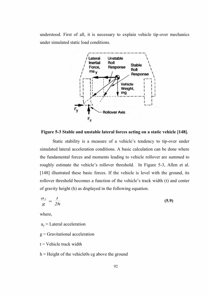
Figure 5-3 Stable and unstable lateral forces acting on a static vehicle [148]. .............. 92
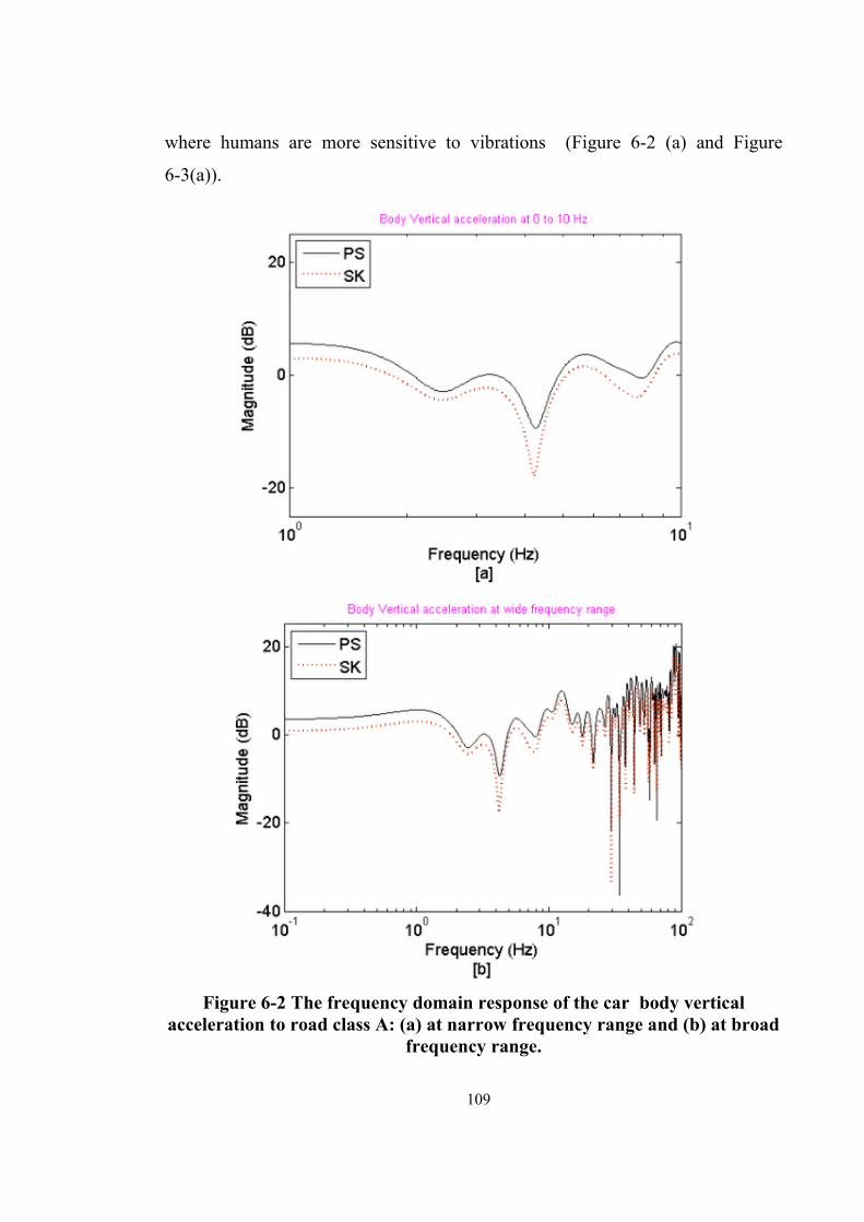
Figure 6-1 Simulink model............................................................................................107 Figure 6-2 The frequency domain response of the car body vertical acceleration to road class A: (a) at narrow frequency range and (b) at broad frequency range. ......... 109
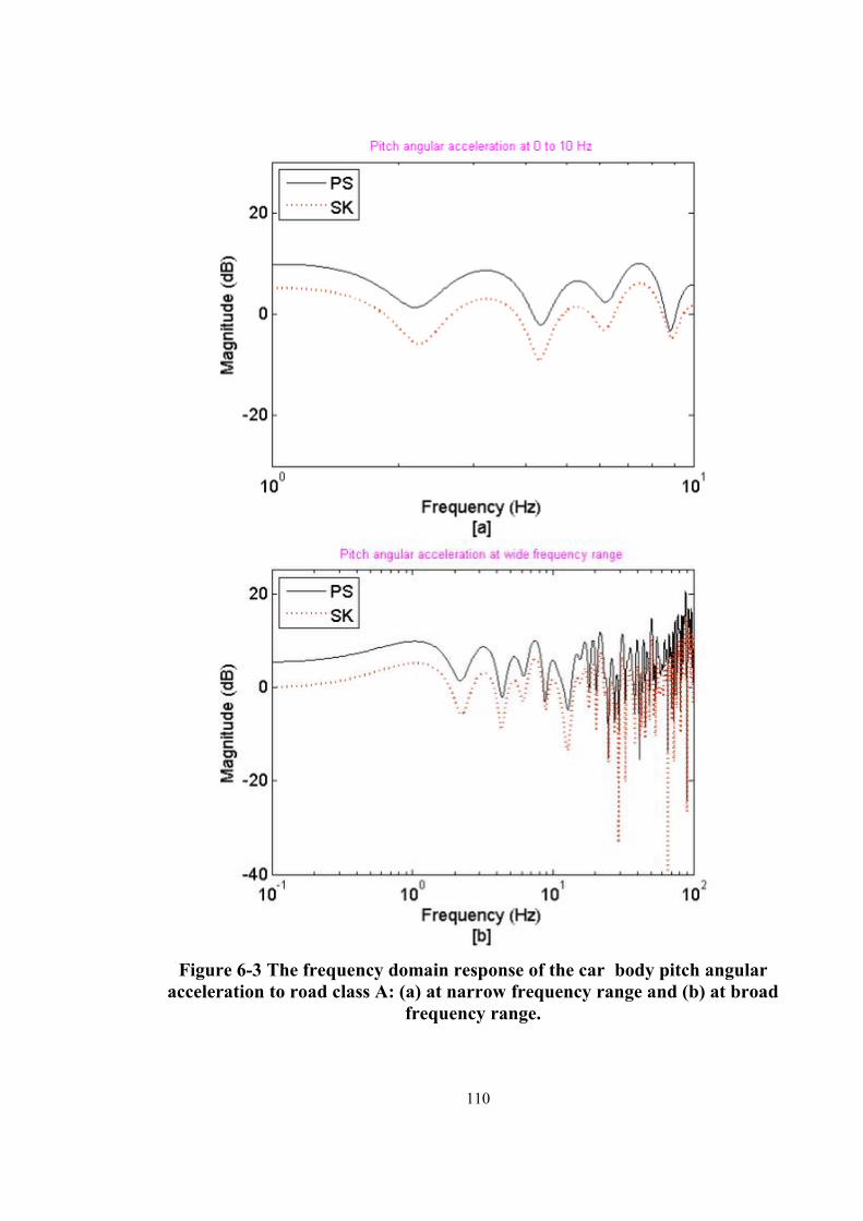
Figure 6-3 The frequency domain response of the car body pitch angular acceleration to road class A: (a) at narrow frequency range and (b) at broad frequency range. ..... 110
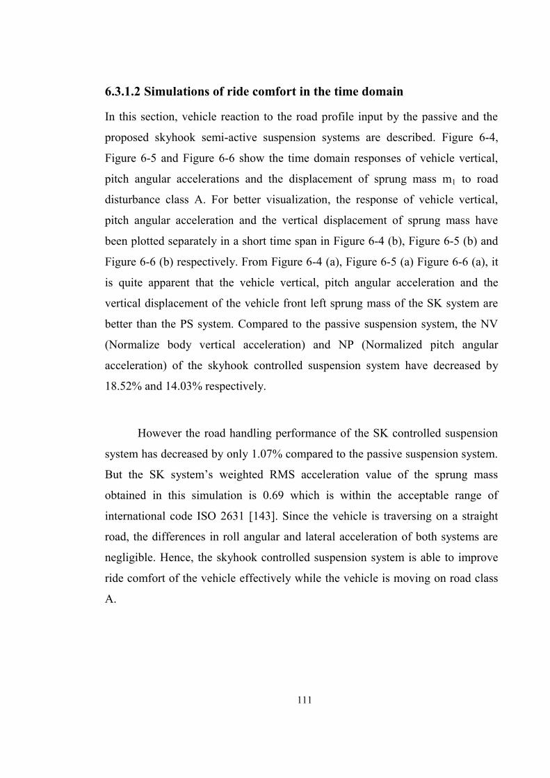
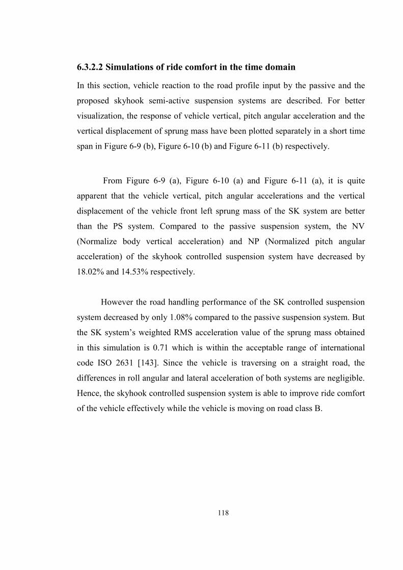
Figure 6-4 The time domain response of vehicle body vertical acceleration to road class A: (a) full trajectory and (b) short time span. ............................................................... 112
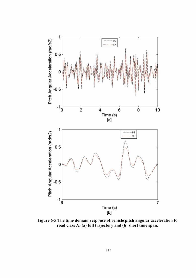
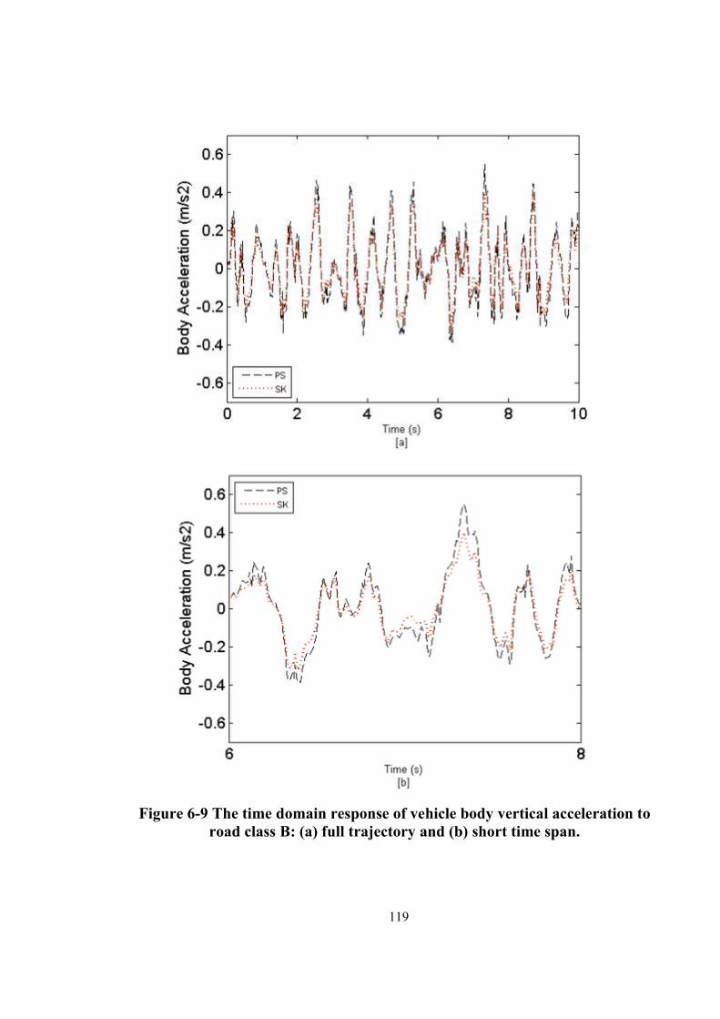
Figure 6-5 The time domain response of vehicle pitch angular acceleration to road class A: (a) full trajectory and (b) short time span. ............................................................... 113
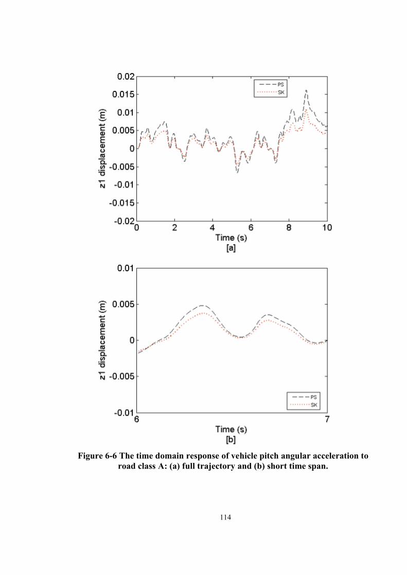
Figure 6-6 The time domain response of vehicle pitch angular acceleration to road class A: (a) full trajectory and (b) short time span. ............................................................... 114
Figure 6-7 The frequency domain response of the car body vertical acceleration to road class B: (a) at narrow frequency range and (b) at broad frequency range. ......... 116
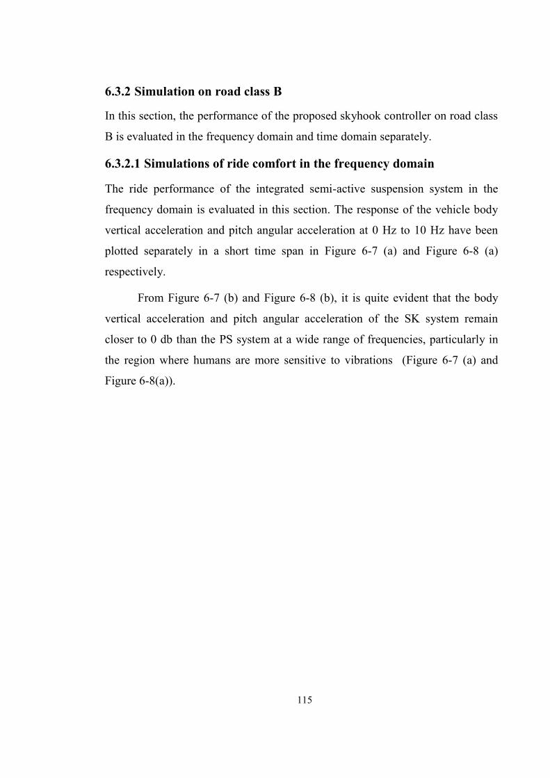
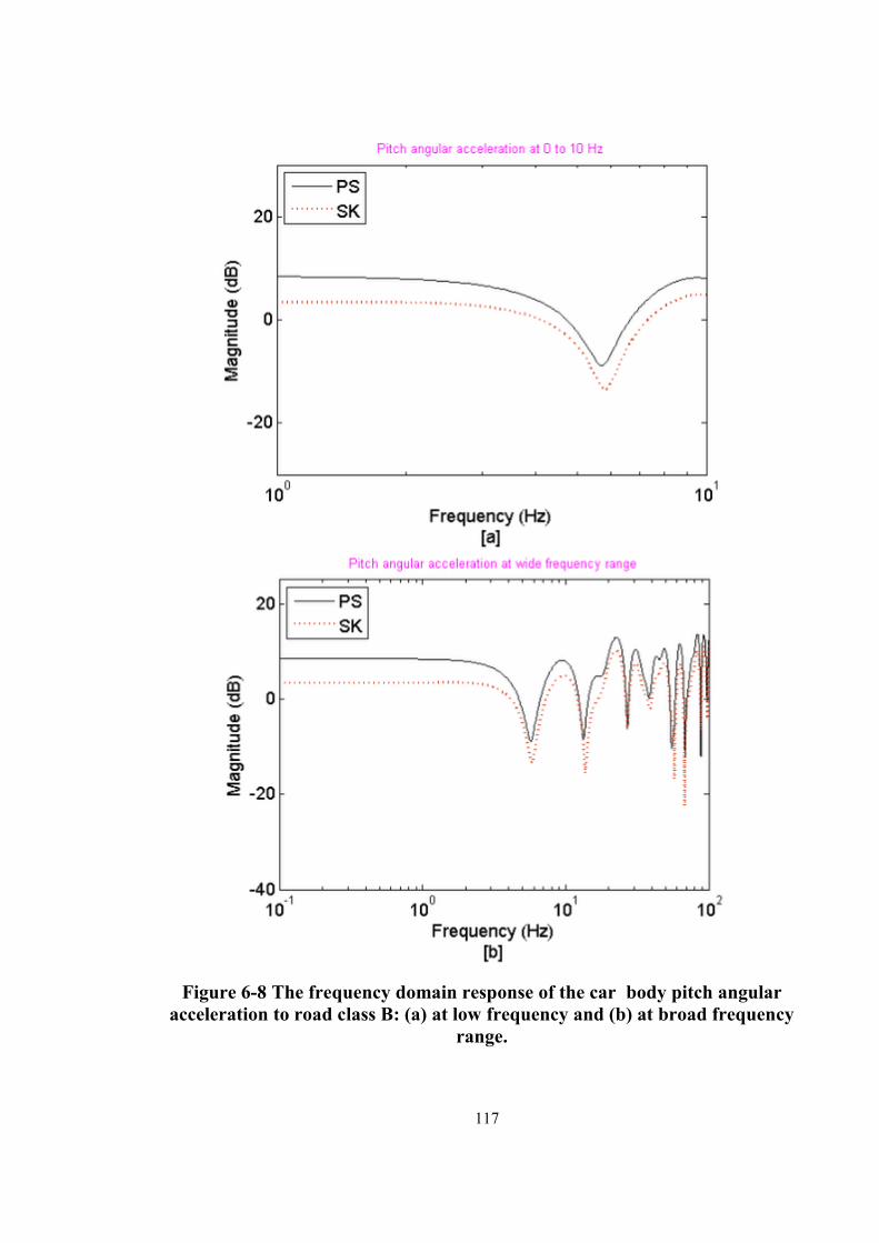
Figure 6-8 The frequency domain response of the car body pitch angular acceleration to road class B: (a) at low frequency and (b) at broad frequency range. ..................... 117
Figure 6-9 The time domain response of vehicle body vertical acceleration to road class B: (a) full trajectory and (b) short time span. ............................................................... 119
Figure 6-10 The time domain response of vehicle pitch angular acceleration to road class B: (a) full trajectory and (b) short time span. ....................................................... 120
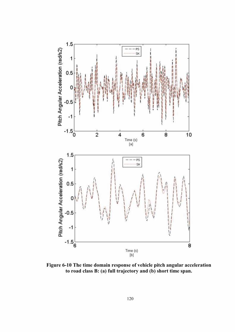
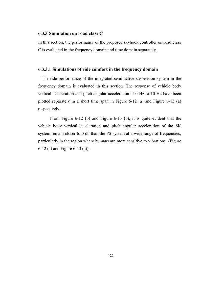
Figure 6-11 The time domain response of the vehicle sprung mass m1 vertical displacement to road class B: (a) full trajectory and (b) short time span. ................... 121
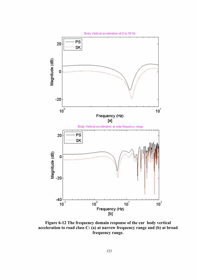
Figure 6-12 The frequency domain response of the car body vertical acceleration to road class C: (a) at narrow frequency range and (b) at broad frequency range. ......... 123
Figure 6-13 The frequency domain response of the car body pitch angular acceleration to road class C: (a) at narrow frequency range and (b) at broad frequency range. ..... 124
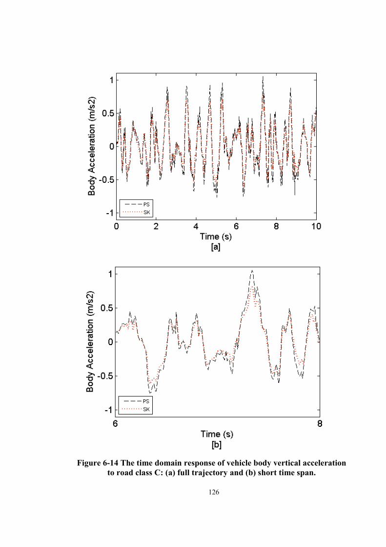
Figure 6-14 The time domain response of vehicle body vertical acceleration to road class C: (a) full trajectory and (b) short time span. ....................................................... 126
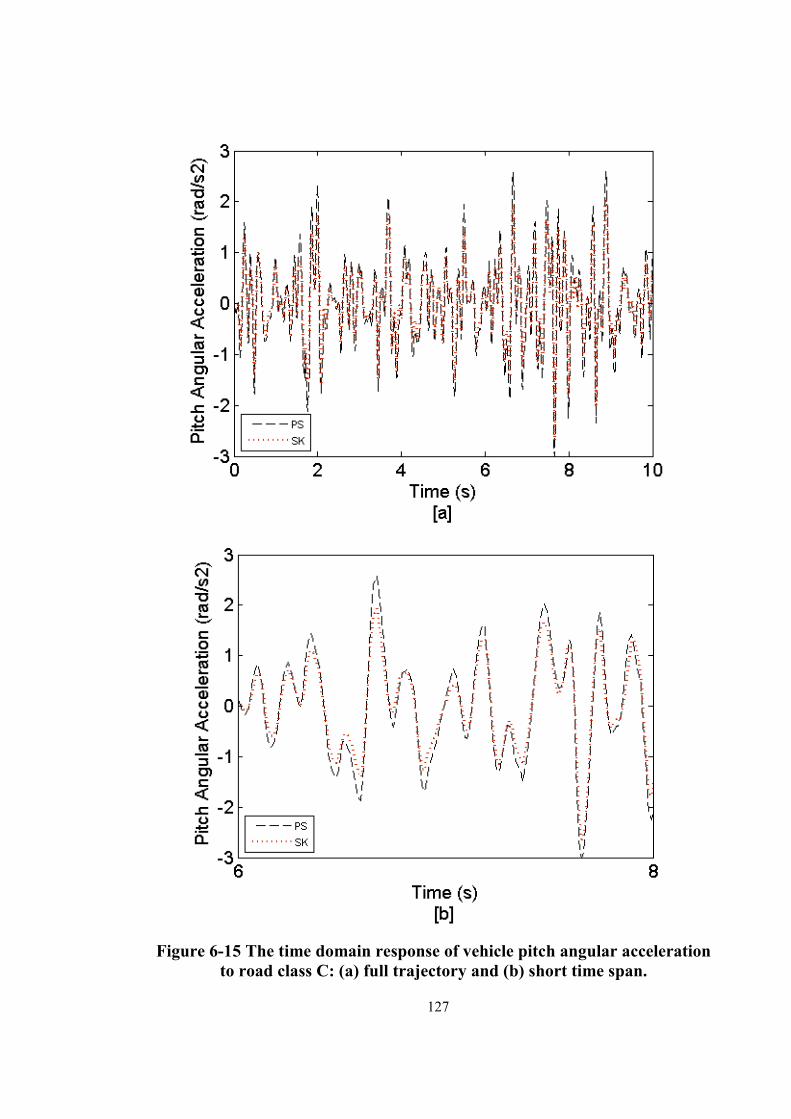
Figure 6-15 The time domain response of vehicle pitch angular acceleration to road class C: (a) full trajectory and (b) short time span. ....................................................... 127
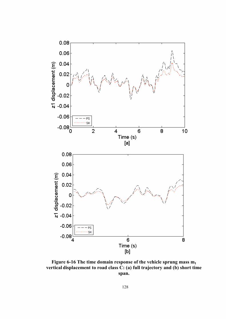
Figure 6-16 The time domain response of the vehicle sprung mass m1 vertical displacement to road class C: (a) full trajectory and (b) short time span. ................... 128
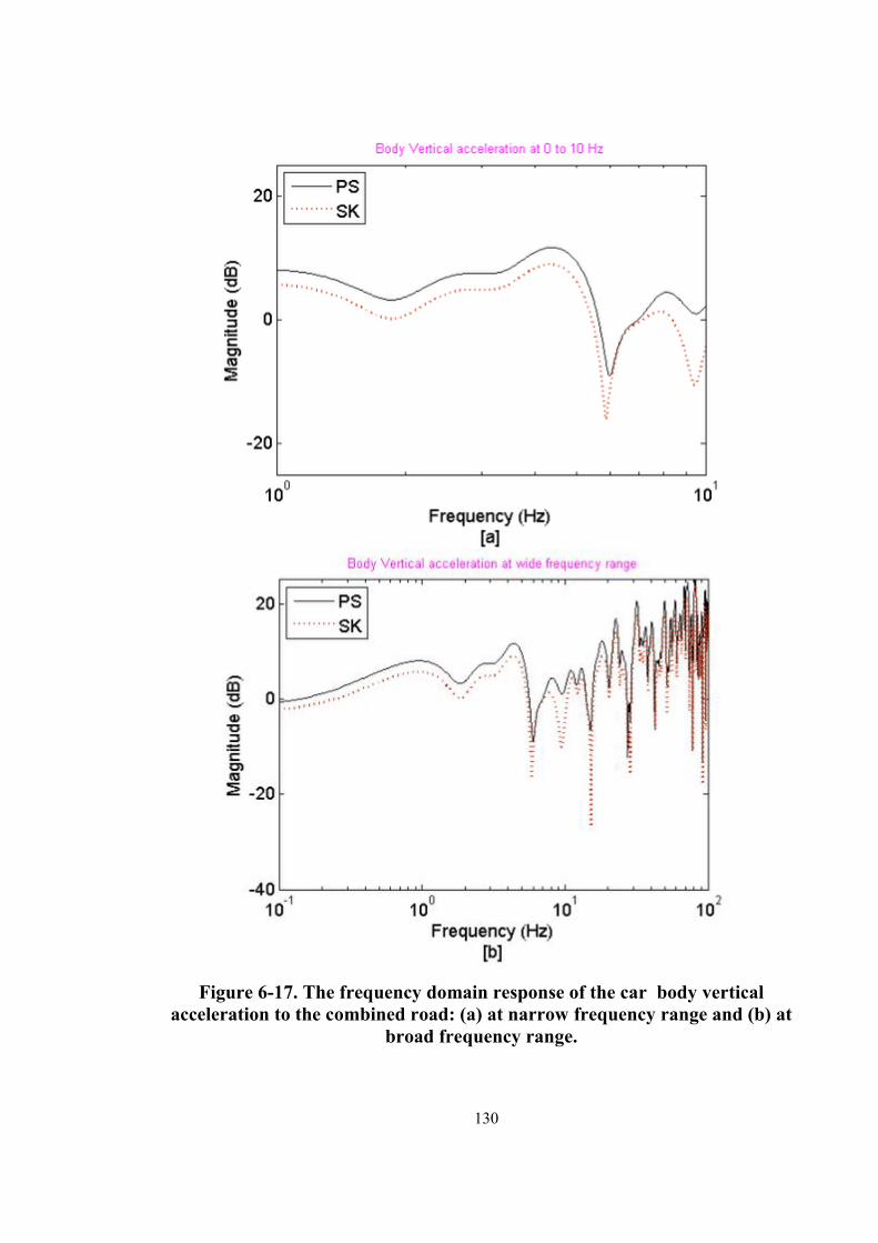
Figure 6-17. The frequency domain response of the car body vertical acceleration to the combined road: (a) at narrow frequency range and (b) at broad frequency range. ....................................................................................................................................... 130
xiii
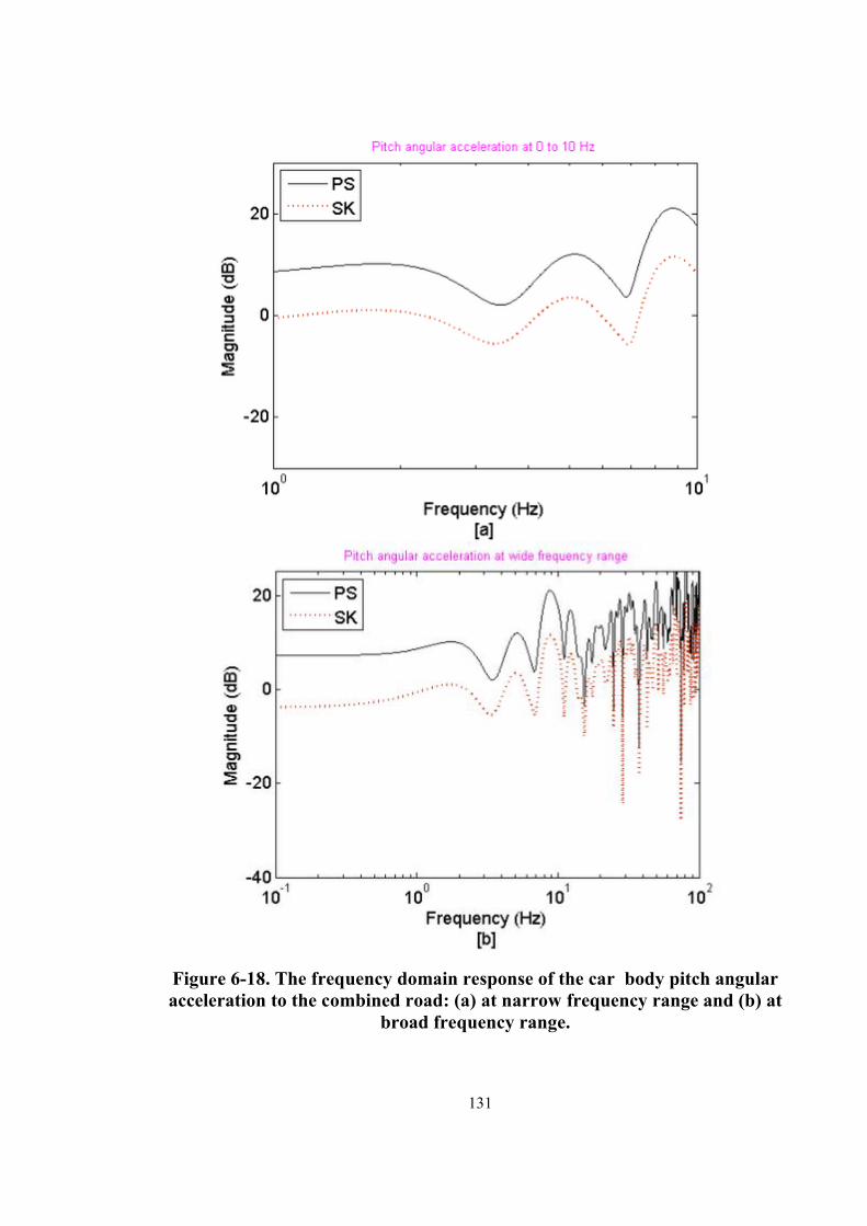
Figure 6-18. The frequency domain response of the car body pitch angular acceleration to the combined road: (a) at narrow frequency range and (b) at broad frequency range. ........................................................................................................... 131
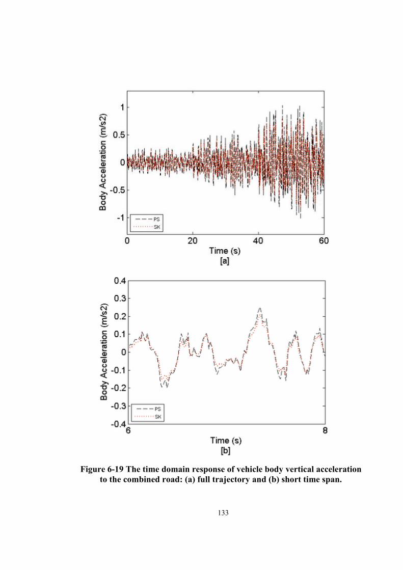
Figure 6-19 The time domain response of vehicle body vertical acceleration to the combined road: (a) full trajectory and (b) short time span. ......................................... 133
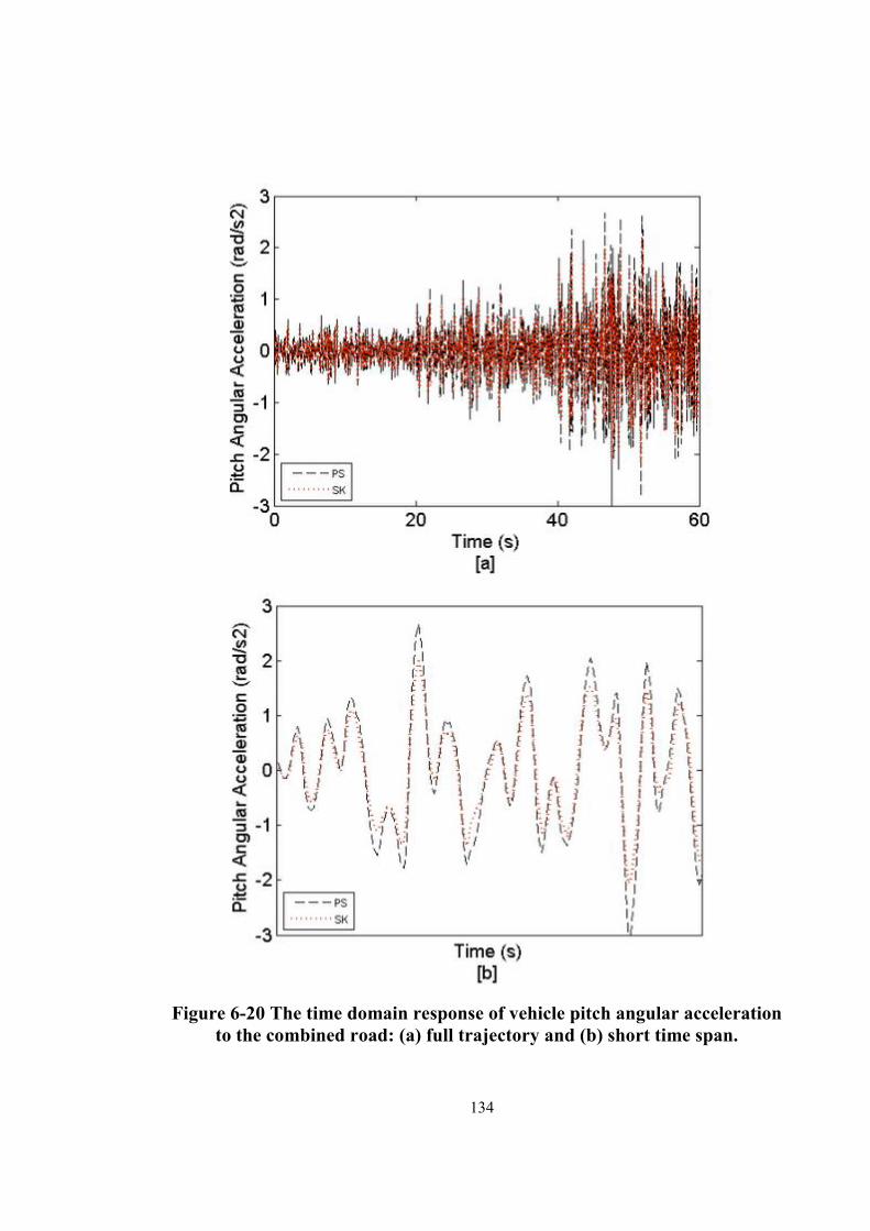
Figure 6-20 The time domain response of vehicle pitch angular acceleration to the combined road: (a) full trajectory and (b) short time span. ......................................... 134
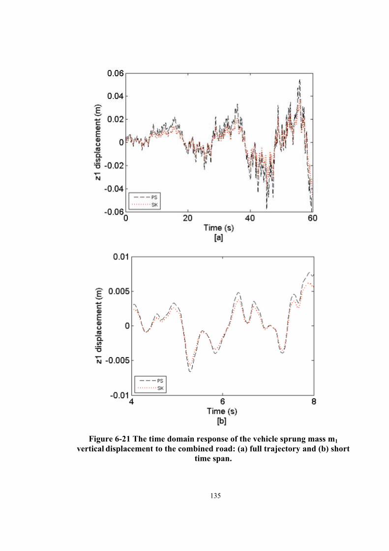
Figure 6-21 The time domain response of the vehicle sprung mass m1 vertical displacement to the combined road: (a) full trajectory and (b) short time span. ........ 135
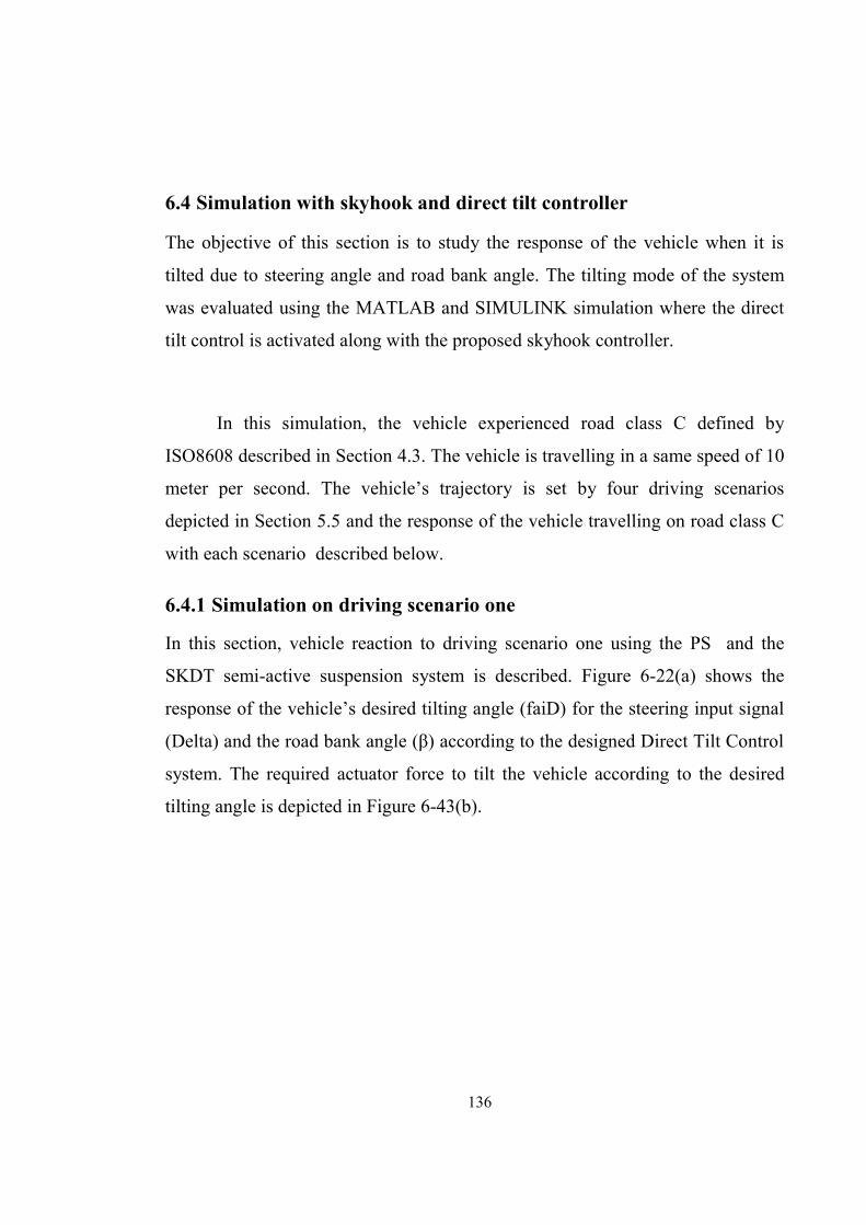
Figure 6-22 The response of steering and bank angle in driving scenario one: (a) Desired tilting angle (b) Required actuator force. ........................................................ 137
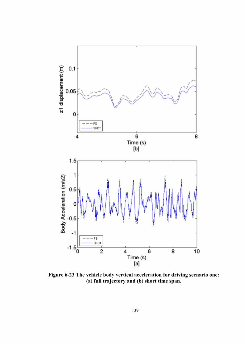
Figure 6-23 The vehicle body vertical acceleration for driving scenario one: (a) full trajectory and (b) short time span. ............................................................................... 139
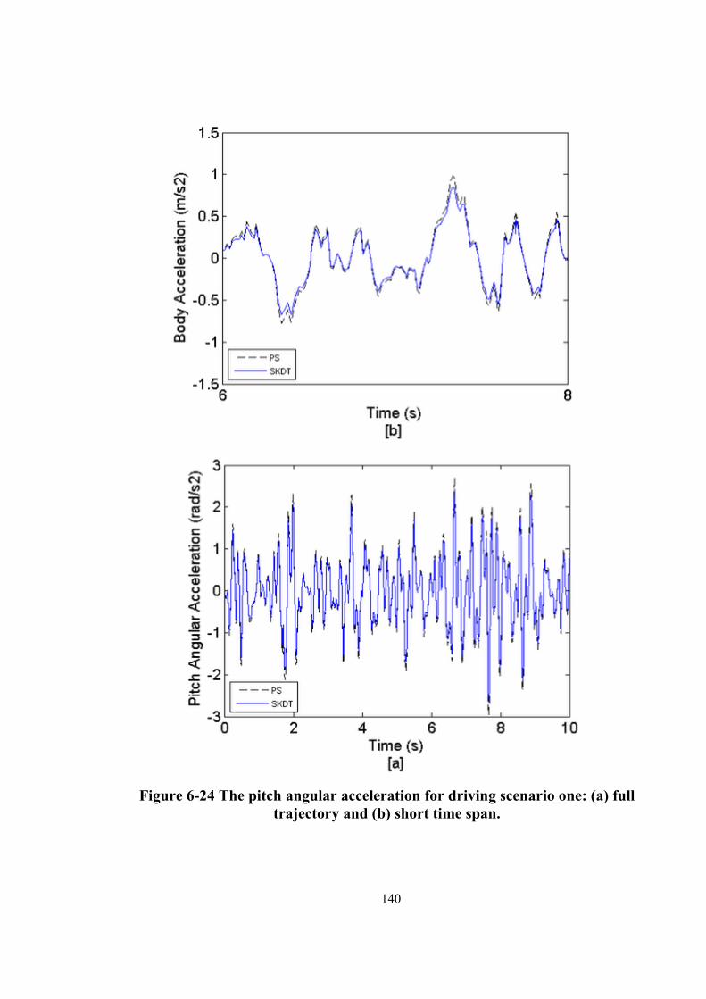
Figure 6-24 The pitch angular acceleration for driving scenario one: (a) full trajectory and (b) short time span. ................................................................................................ 140
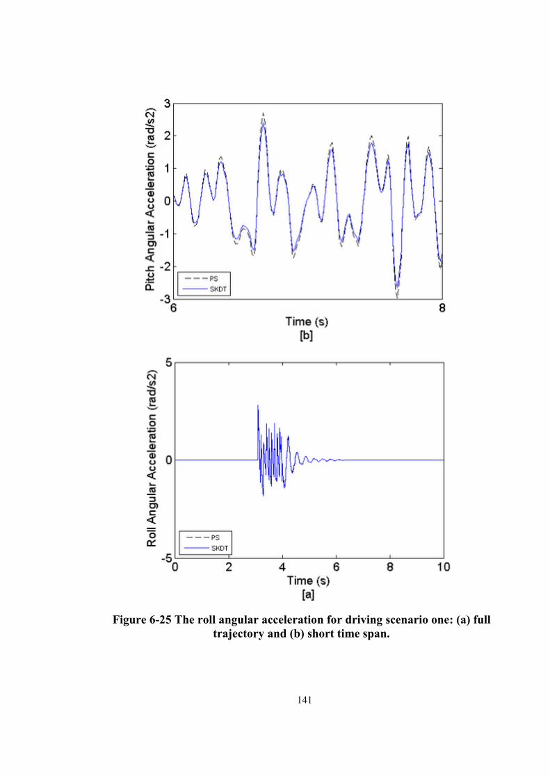
Figure 6-25 The roll angular acceleration for driving scenario one: (a) full trajectory and (b) short time span. ....................................................................................................... 141
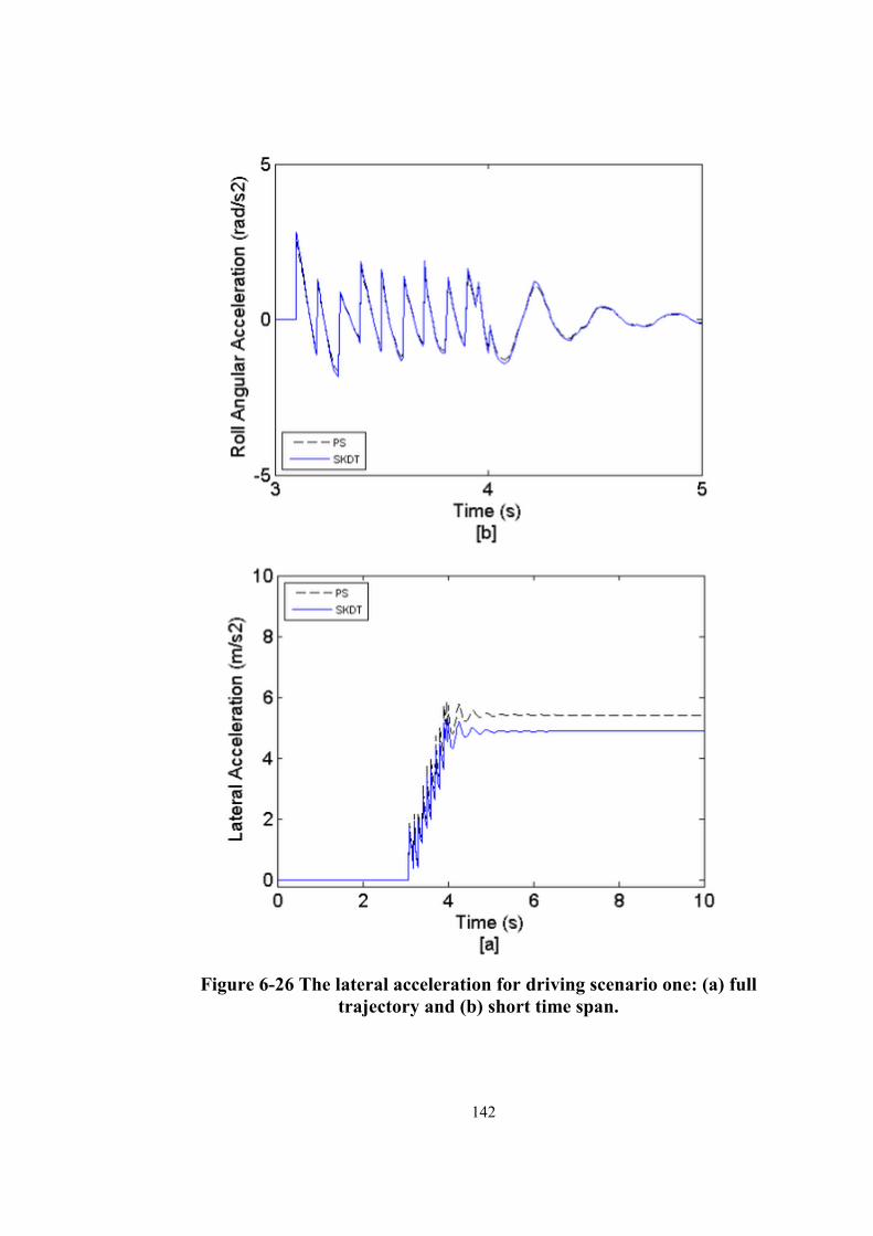
Figure 6-26 The lateral acceleration for driving scenario one: (a) full trajectory and (b) short time span. ............................................................................................................ 142
Figure 6-27 The vehicle sprung mass m1‘s vertical displacement for driving scenario one: (a) full trajectory and (b) short time span. ........................................................... 143
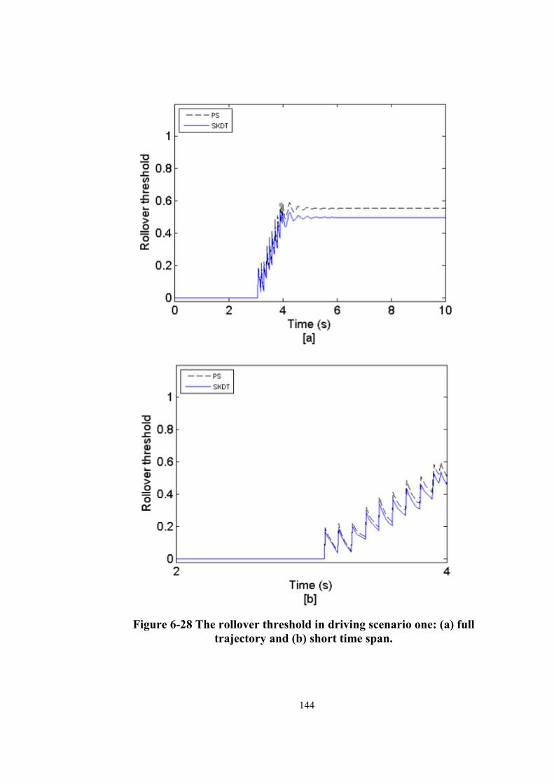
Figure 6-28 The rollover threshold in driving scenario one: (a) full trajectory and (b) short time span. ............................................................................................................ 144
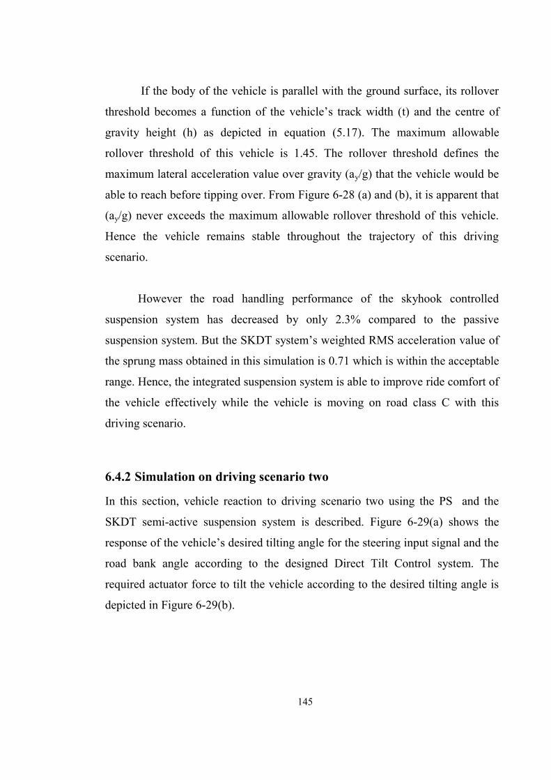
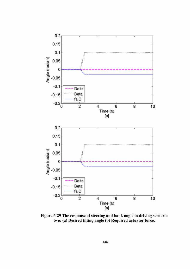
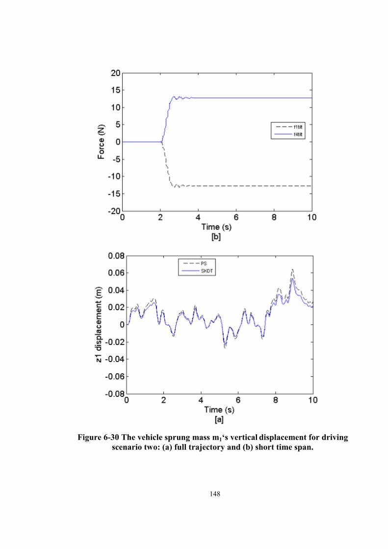
Figure 6-29 The response of steering and bank angle in driving scenario two: (a) Desired tilting angle (b) Required actuator force. ........................................................ 146
Figure 6-30 The vehicle sprung mass m1‘s vertical displacement for driving scenario two: (a) full trajectory and (b) short time span. ........................................................... 148
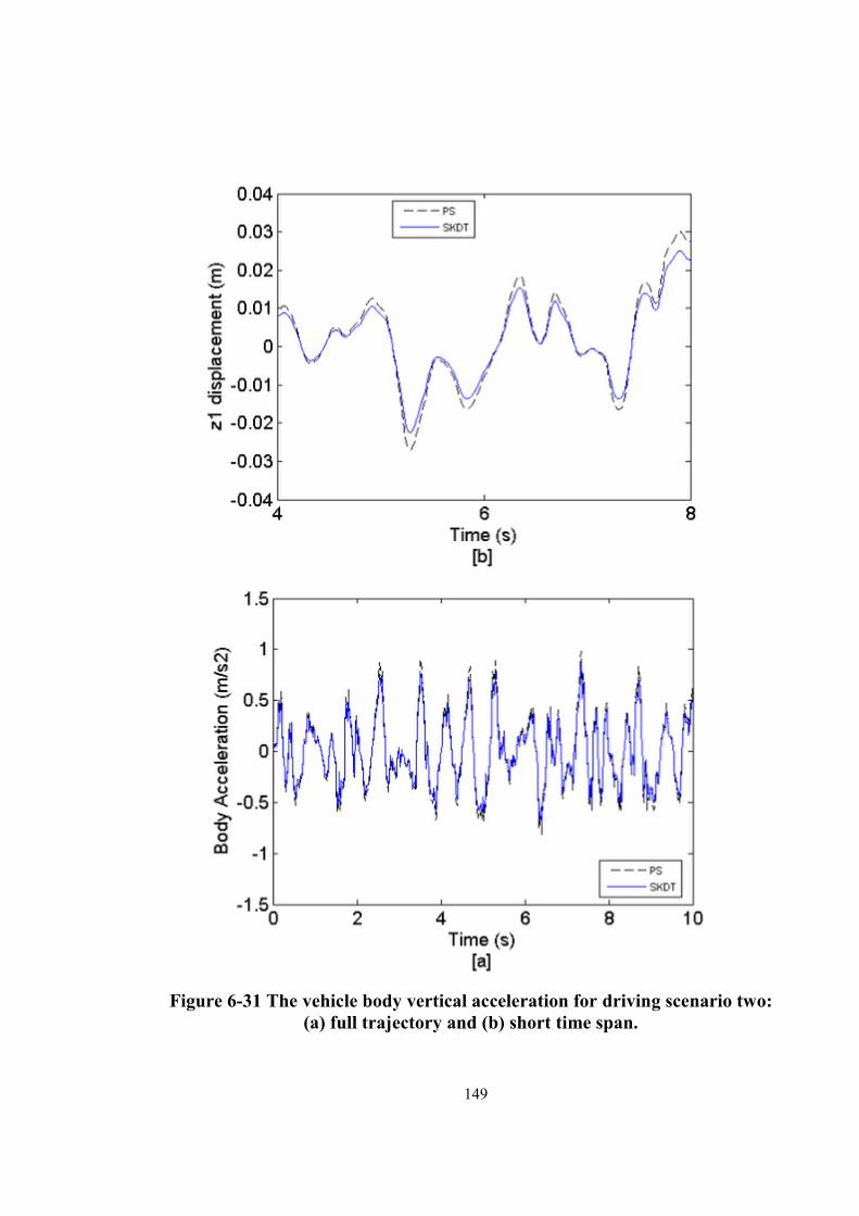
Figure 6-31 The vehicle body vertical acceleration for driving scenario two: (a) full trajectory and (b) short time span. ............................................................................... 149
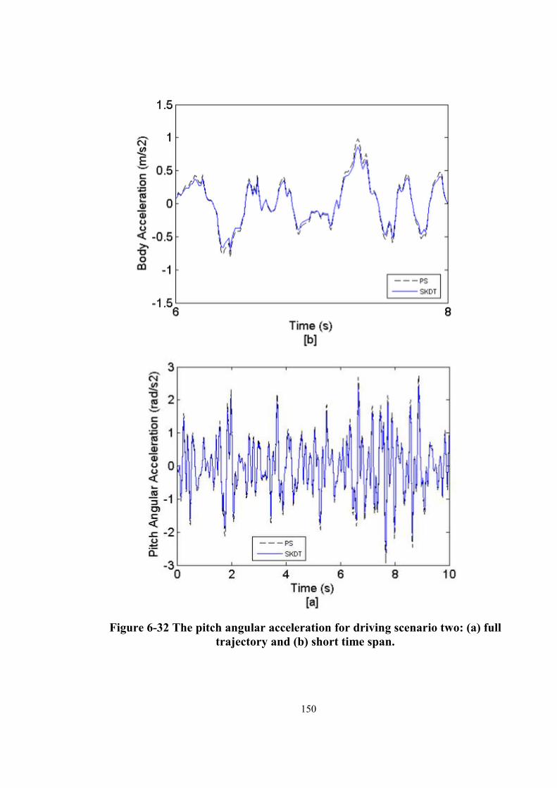
Figure 6-32 The pitch angular acceleration for driving scenario two: (a) full trajectory and (b) short time span. ................................................................................................ 150
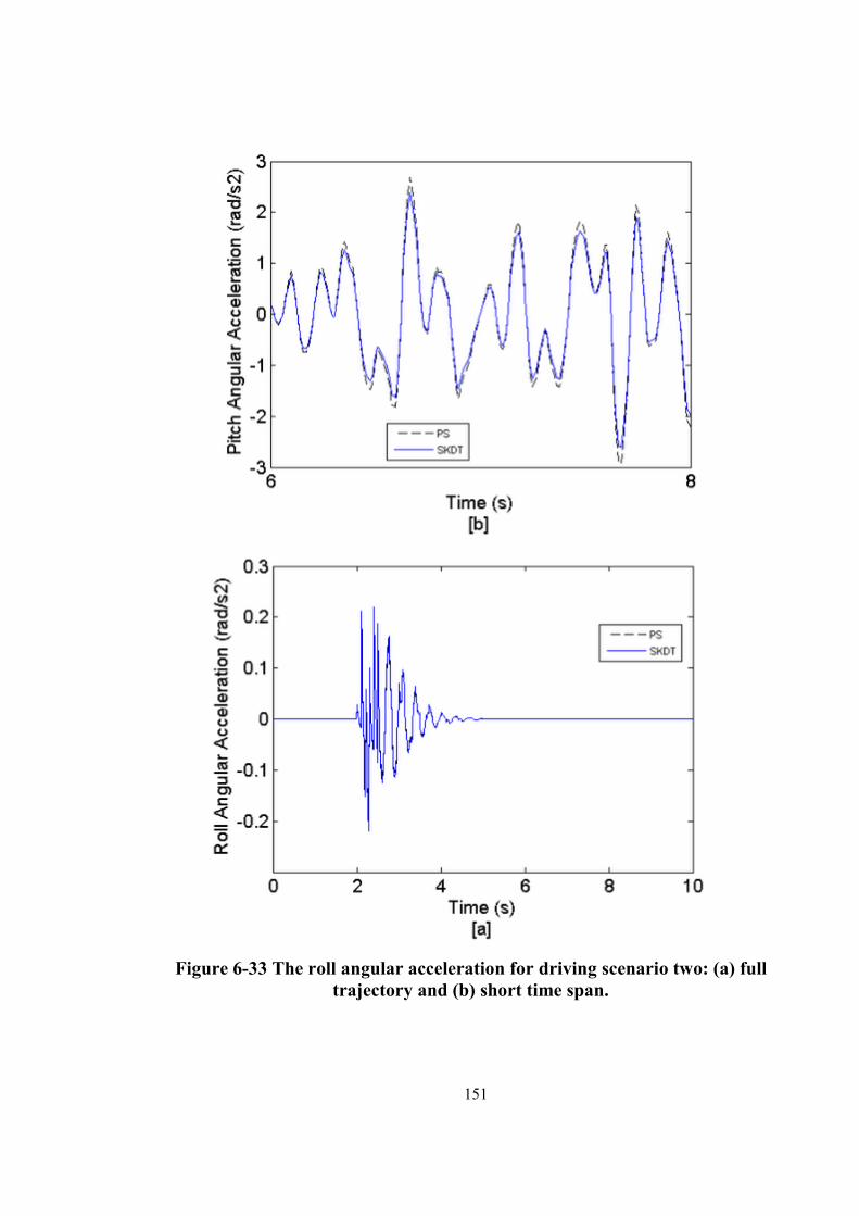
Figure 6-33 The roll angular acceleration for driving scenario two: (a) full trajectory and (b) short time span. ....................................................................................................... 151
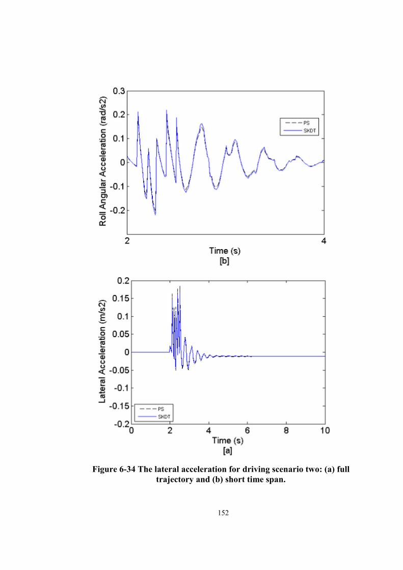
Figure 6-34 The lateral acceleration for driving scenario two: (a) full trajectory and (b) short time span. ............................................................................................................ 152
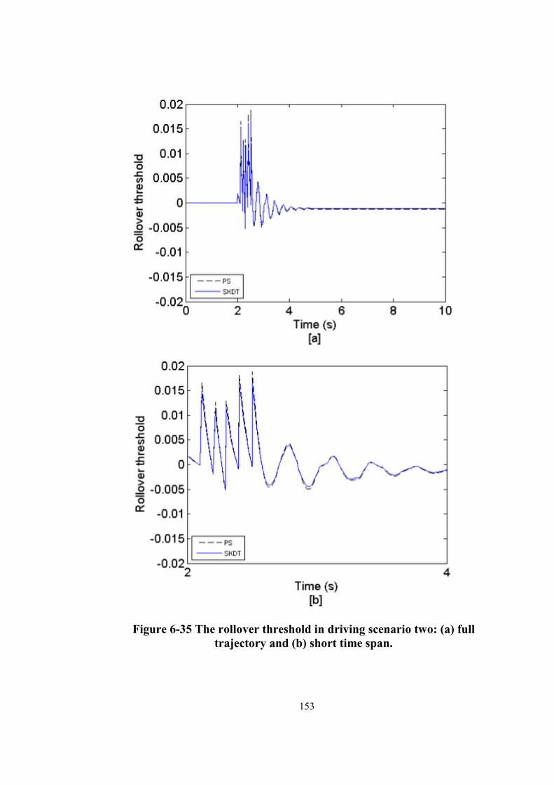
Figure 6-35 The rollover threshold in driving scenario two: (a) full trajectory and (b) short time span. ............................................................................................................ 153
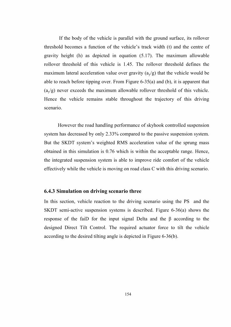
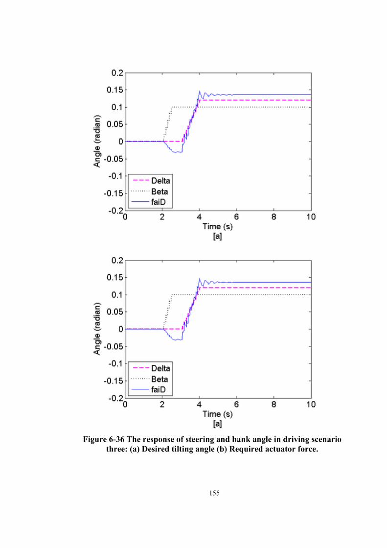
Figure 6-36 The response of steering and bank angle in driving scenario three: (a) Desired tilting angle (b) Required actuator force. ........................................................ 155
Figure 6-37 The vehicle sprung mass m1‘s vertical displacement for driving scenario three: (a) full trajectory and (b) short time span. ......................................................... 157
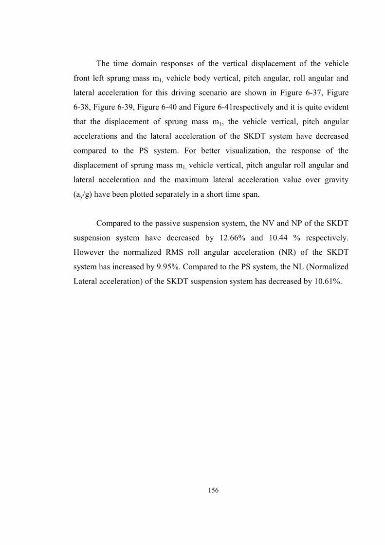
Figure 6-38 The vehicle body vertical acceleration for driving scenario three: (a) full trajectory and (b) short time span. ............................................................................... 158
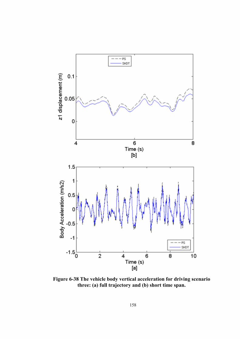
Figure 6-39 The pitch angular acceleration for driving scenario three: (a) full trajectory and (b) short time span. ................................................................................................ 159
xiv
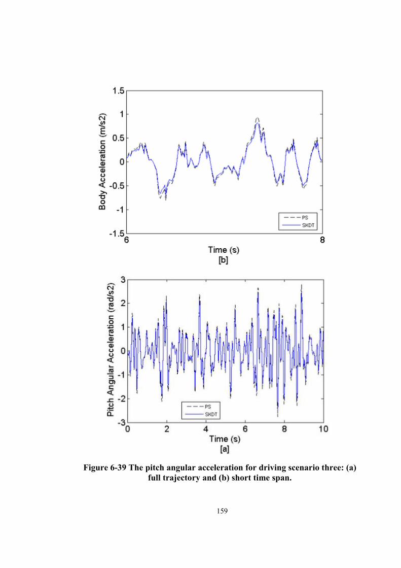
Figure 6-40 The roll angular acceleration for driving scenario three: (a) full trajectory and (b) short time span. ................................................................................................ 160
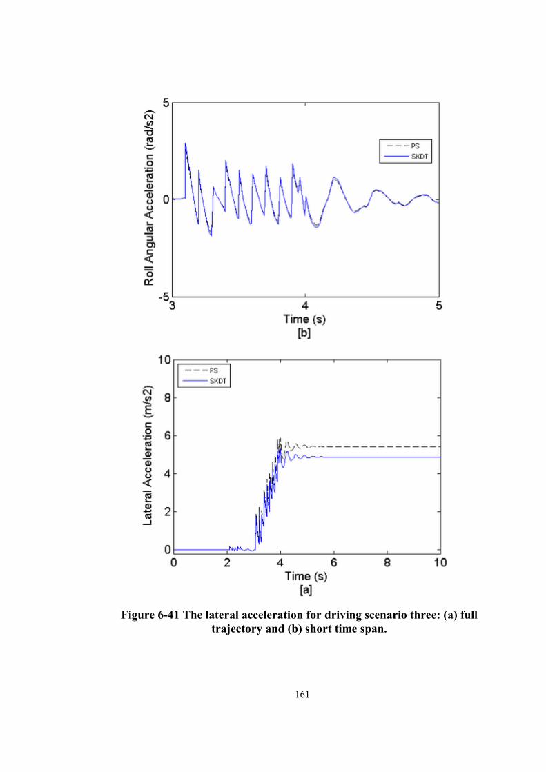
Figure 6-41 The lateral acceleration for driving scenario three: (a) full trajectory and (b) short time span. ............................................................................................................ 161
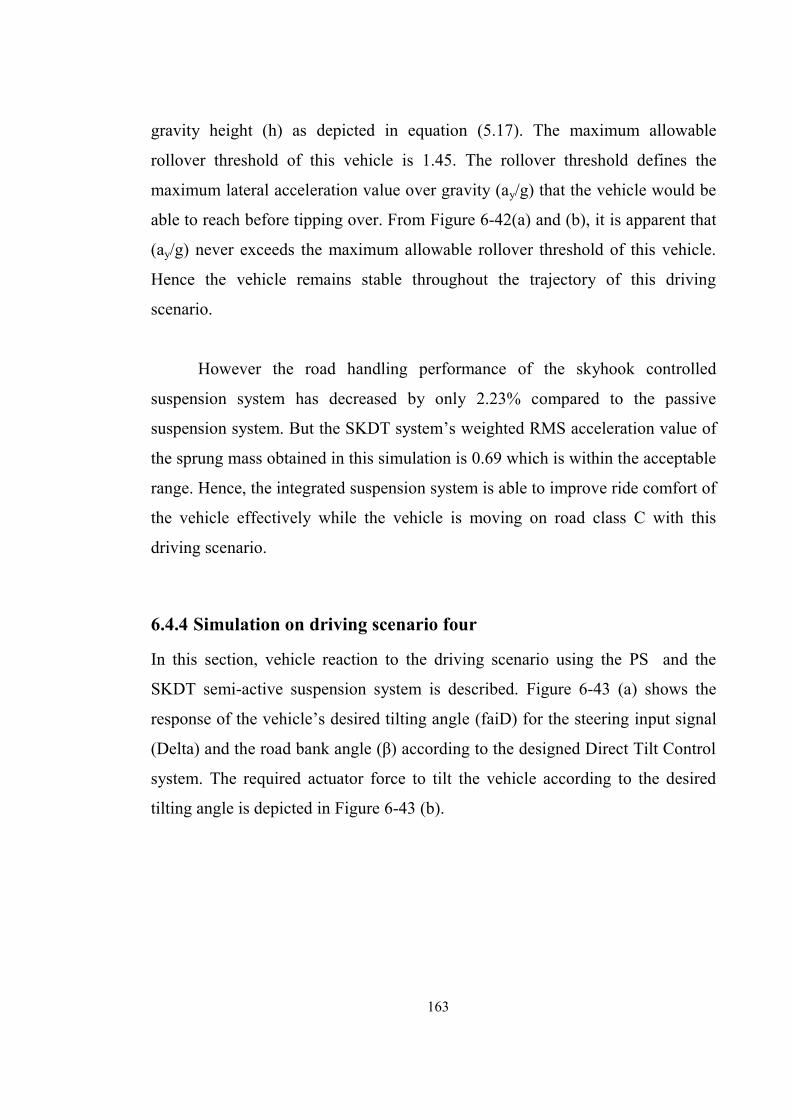
Figure 6-42 Vehicle suspension system........................................................................163 Figure 6-43 The response of steering and bank angle in driving scenario four: (a) Desired tilting angle (b) Required actuator force. ........................................................ 164
Figure 6-44 The vehicle sprung mass m1‘s vertical displacement for driving scenario four: (a) full trajectory and (b) short time span. ........................................................... 166
Figure 6-45 The vehicle body vertical acceleration for driving scenario four: (a) full trajectory and (b) short time span. ............................................................................... 167
Figure 6-46 The pitch angular acceleration for driving scenario four: (a) full trajectory and (b) short time span. ................................................................................................ 168
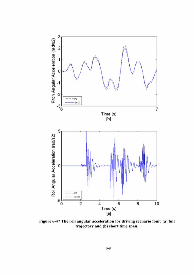
Figure 6-47 The roll angular acceleration for driving scenario four: (a) full trajectory and (b) short time span. ................................................................................................ 169
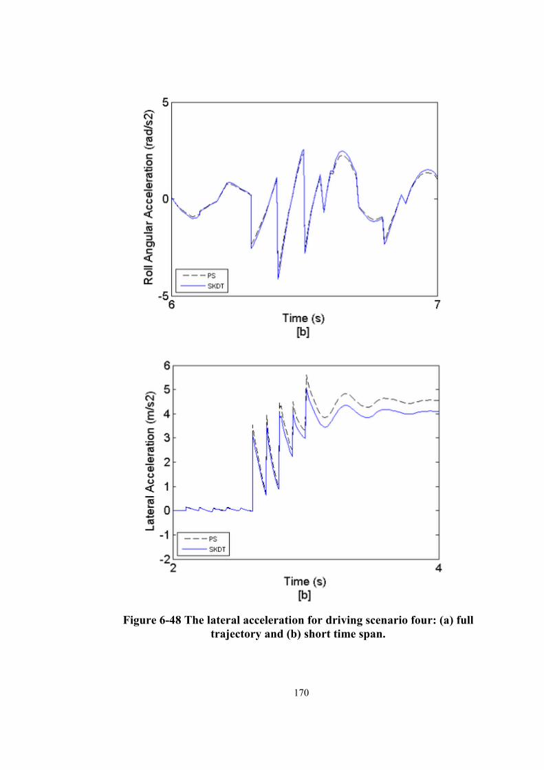
Figure 6-48 The lateral acceleration for driving scenario four: (a) full trajectory and (b) short time span. ............................................................................................................ 170
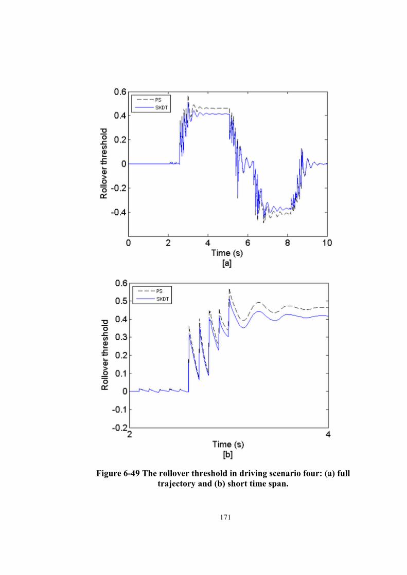
Figure 6-49 The rollover threshold in driving scenario four: (a) full trajectory and (b) short time span. ............................................................................................................ 171
Figure 6-50. The frequency domain response of the car body vertical acceleration: (a) at narrow frequency range and (b) at broad frequency range. .................................... 174
Figure 6-51. The frequency domain response of the car body pitch angular acceleration: (a) at narrow frequency range and (b) at broad frequency range. ........ 175
Figure 6-52. The frequency domain response of the car body roll angular acceleration: (a) at narrow frequency range and (b) at broad frequency range. .............................. 176
Figure 6-53 Vehicle suspension system.......................................................................179 Figure 6-54 The vehicle body vertical acceleration for driving scenario four and road class C: (a) full trajectory and (b) short time span. ....................................................... 179
Figure 6-55 The pitch angular acceleration for driving scenario four and road class C: (a) full trajectory and (b) short time span. ......................................................................... 180
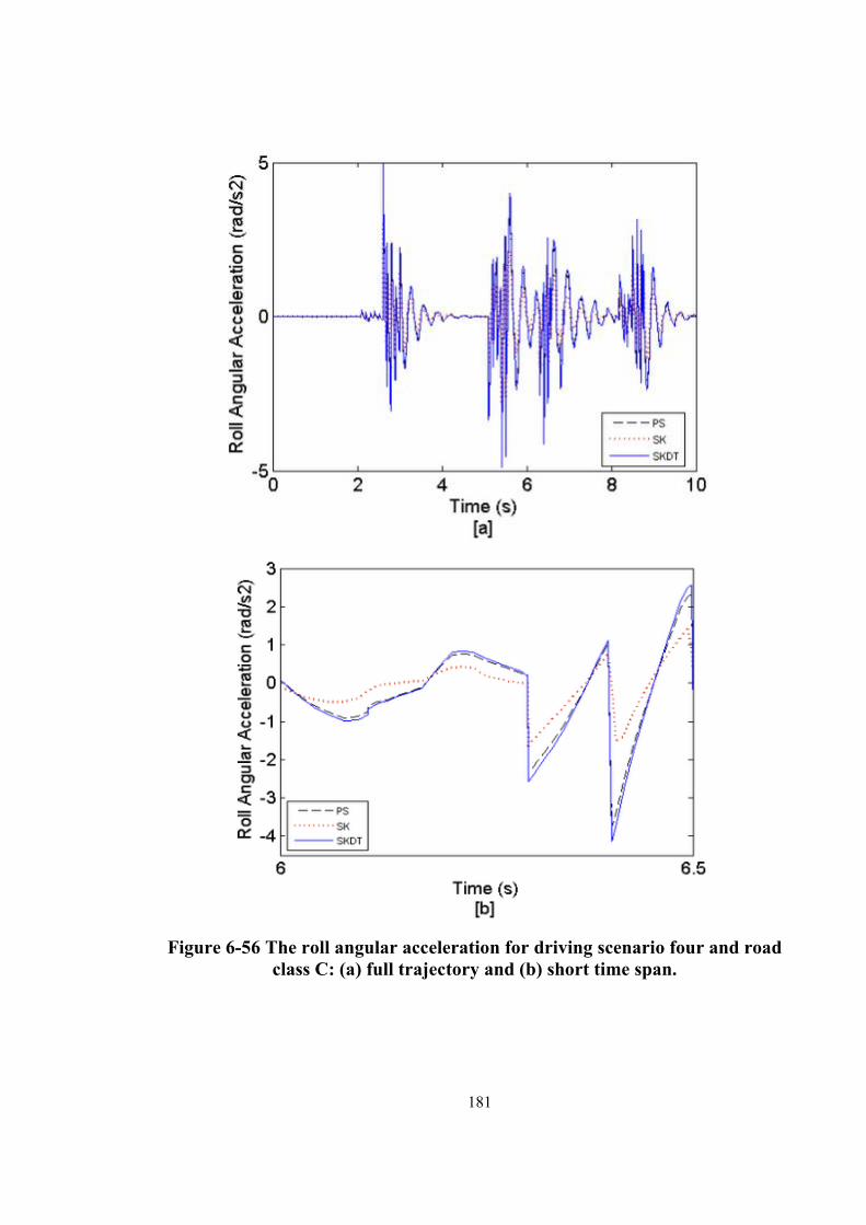
Figure 6-56 The roll angular acceleration for driving scenario four and road class C: (a) full trajectory and (b) short time span. ........................................................................ .181
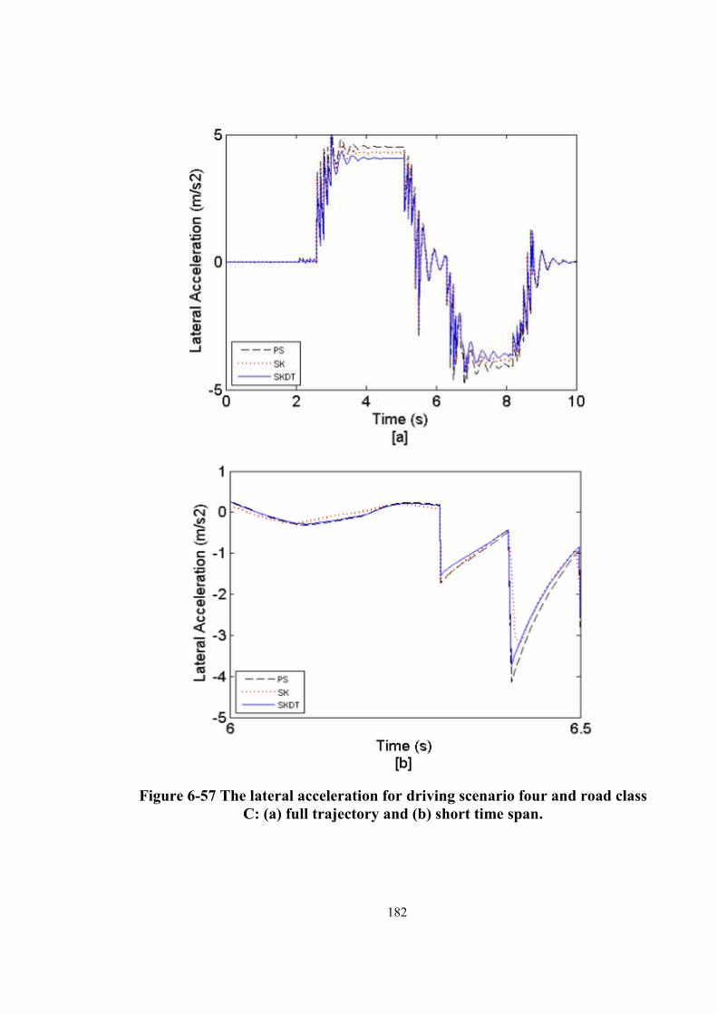
Figure 6-57 The lateral acceleration for driving scenario four and road class C: (a) full trajectory and (b) short time span. ............................................................................... 182
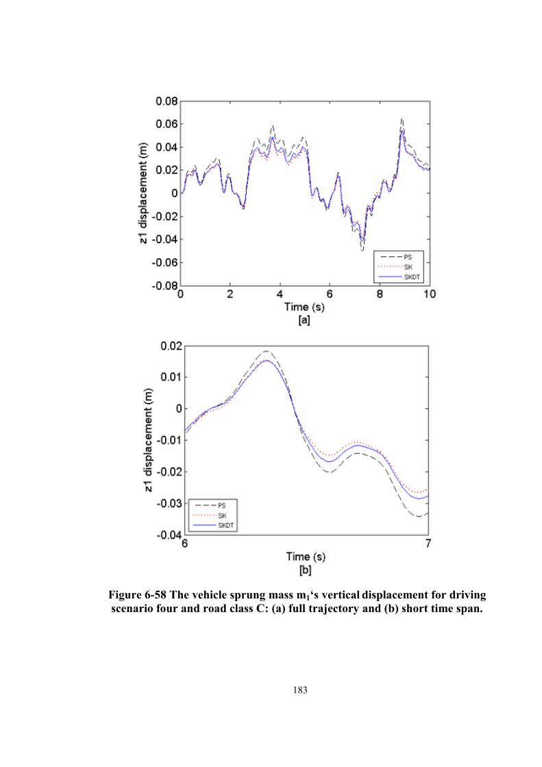
Figure 6-58 The vehicle sprung mass m1‘s vertical displacement for driving scenario four and road class C: (a) full trajectory and (b) short time span. ................................ 183
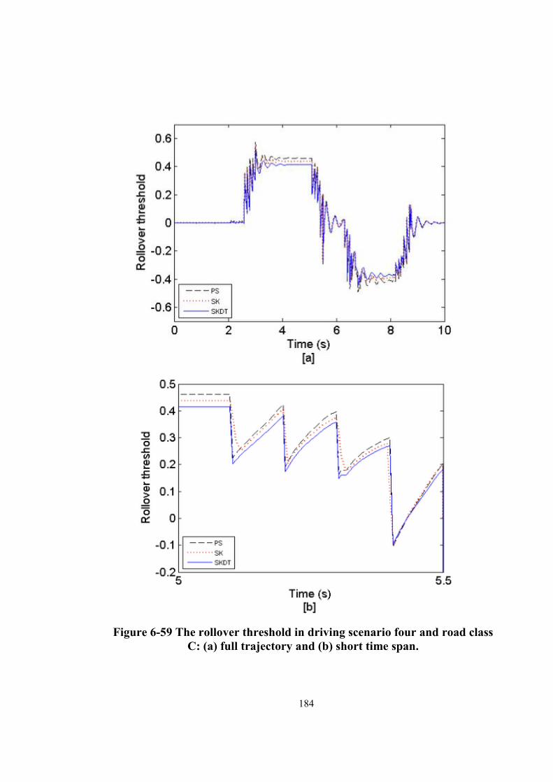
Figure 6-59 The rollover threshold in driving scenario four and road class C: (a) full trajectory and (b) short time span. ............................................................................... 184
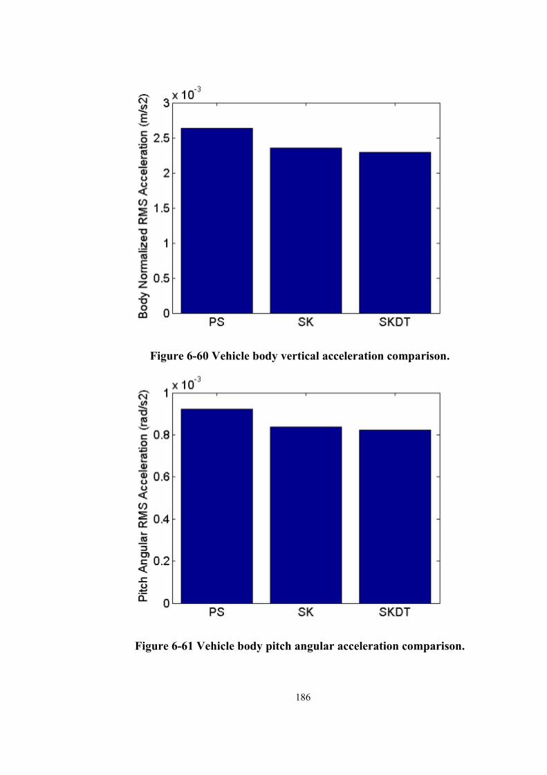
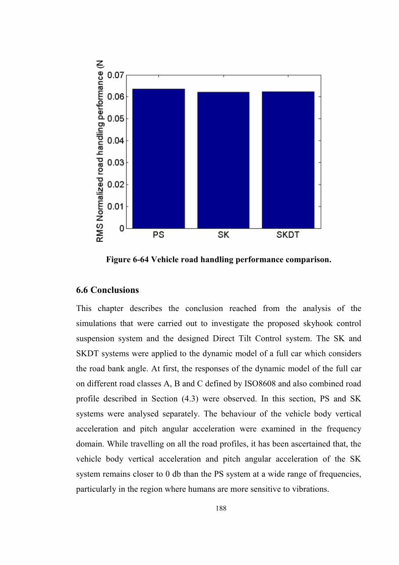
Figure 6-60 Vehicle body vertical acceleration comparison.........................................186 Figure 6-61 Vehicle body pitch acceleration comparison.............................................186 Figure 6-62 Vehicle body roll angular acceleration comparison. ............................. ....187
Figure 6-63.Vehicle body lateral acceleration comparison. ....................................... ..187
Figure 7-1 Quanser Simulink Model..............................................................................194 Figure 7-2 Quanser Intelligent Suspension Plant..........................................................195 Figure 7-3 The vehicle front left sprung mass vertical displacement. .......................... 196
xv
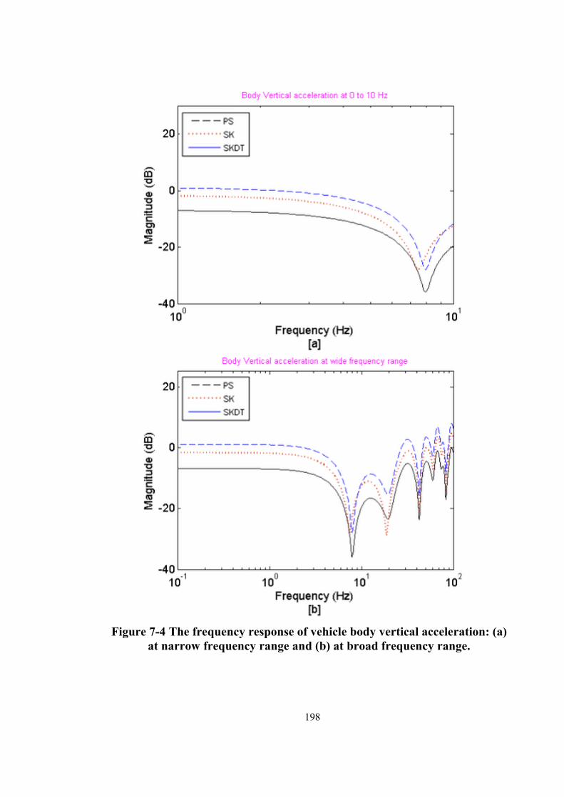
Figure 7-4 The frequency response of vehicle body vertical acceleration: (a) at narrow frequency range and (b) at broad frequency range. .................................................... 198
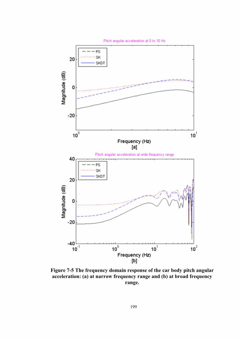
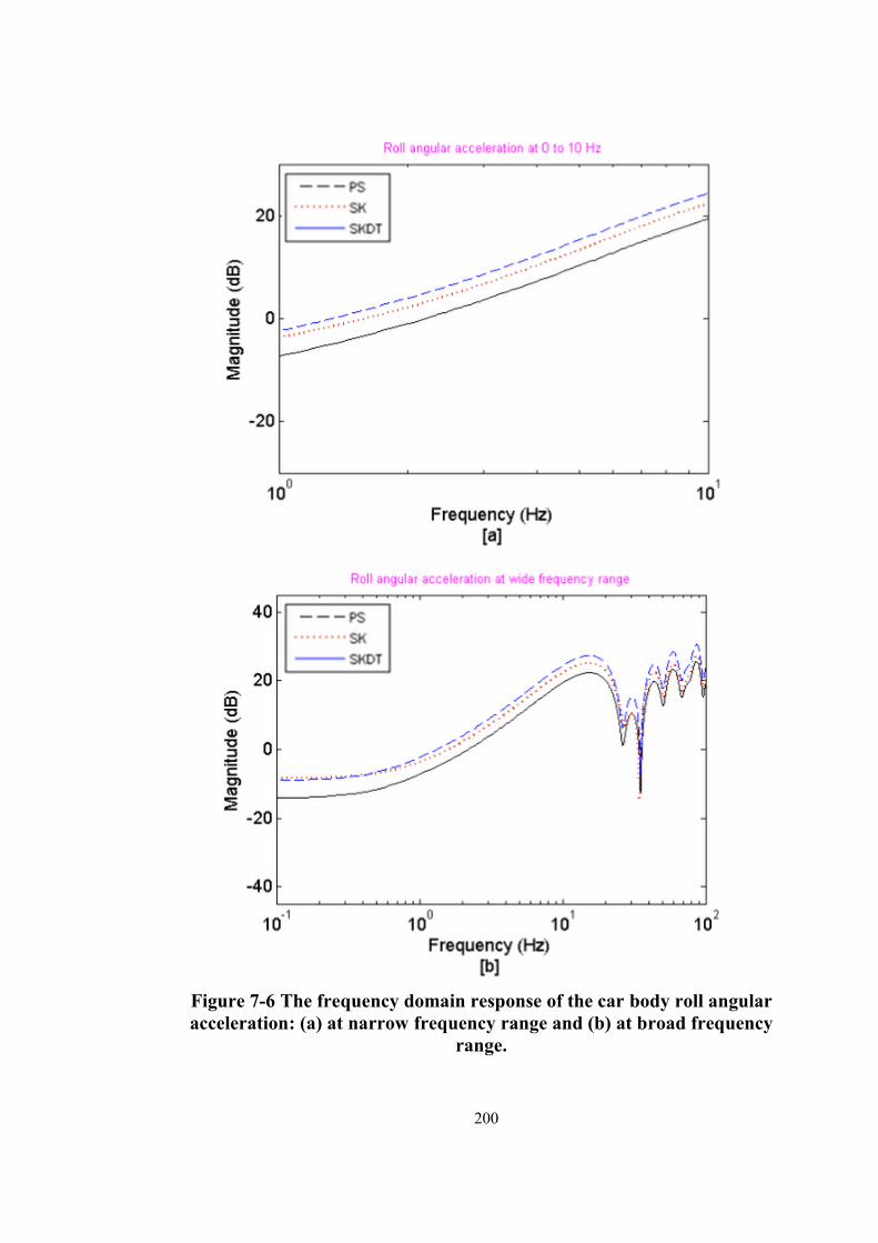
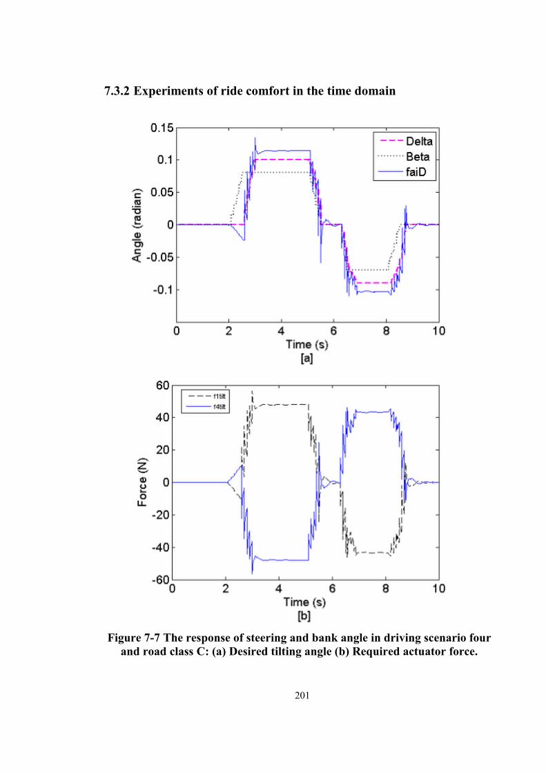
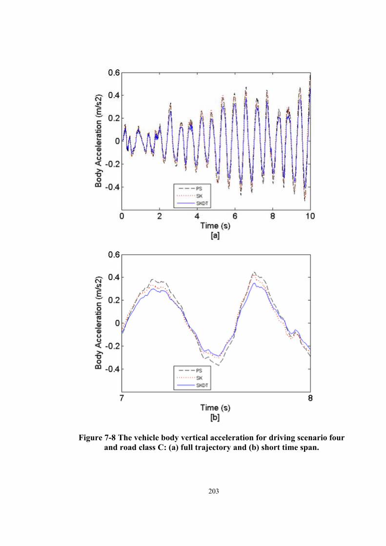
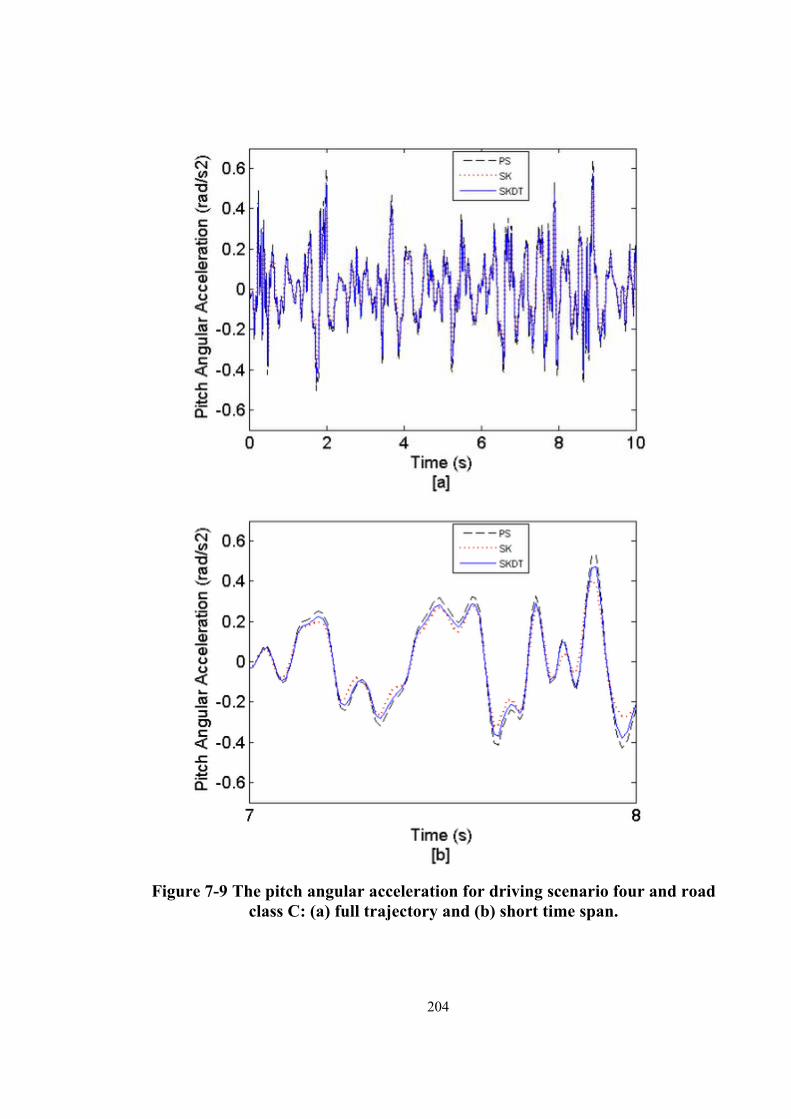
Figure 7-5 The frequency domain response of the car body pitch angular acceleration: (a) at narrow frequency range and (b) at broad frequency range................................199 Figure 7-6 The frequency domain response of the car body roll angular acceleration: (a) at narrow frequency range and (b) at broad frequency range................................200 Figure 7-7 The response of steering and bank angle in driving scenario four and road class C: (a) Desired tilting angle (b) Required actuator force........................................201 Figure 7-8 The vehicle body vertical acceleration for driving scenario four and road class C: (a) full trajectory and (b) short time span.........................................................203 Figure 7-9 The pitch angular acceleration for driving scenario four and road class C: (a) full trajectory and (b) short time span. ......................................................................... 204
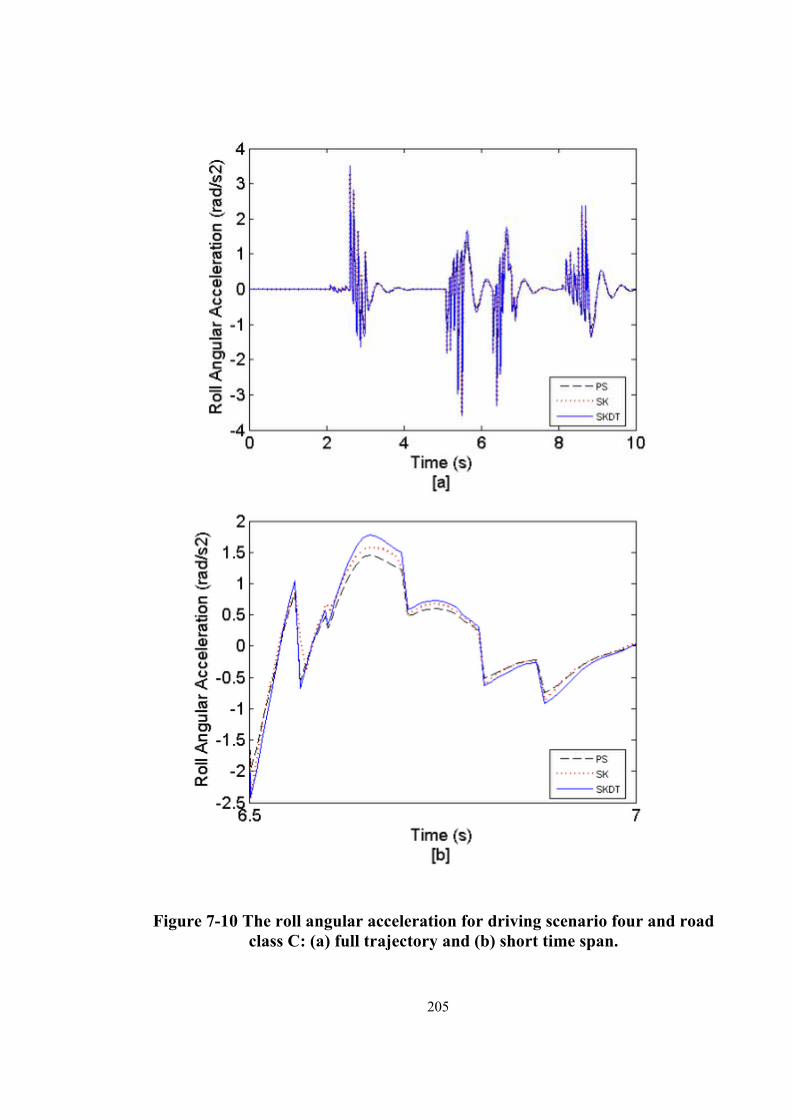
Figure 7-10 The roll angular acceleration for driving scenario four and road class C: (a) full trajectory and (b) short time span. ......................................................................... 205
Figure 7-11 The lateral acceleration for driving scenario four and road class C: (a) full trajectory and (b) short time span. ............................................................................... 206
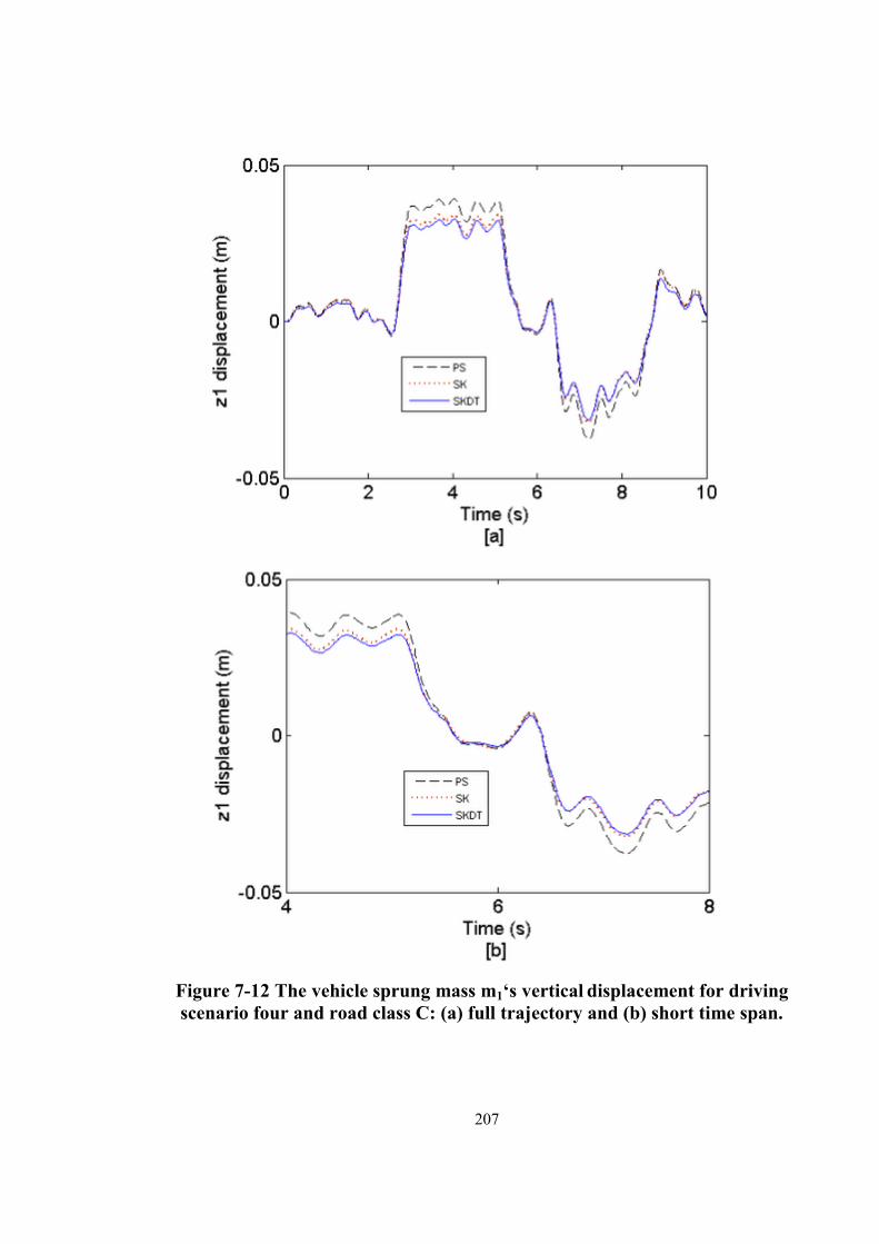
Figure 7-12 The vehicle sprung mass m1‘s vertical displacement for driving scenario four and road class C: (a) full trajectory and (b) short time span. ................................ 207
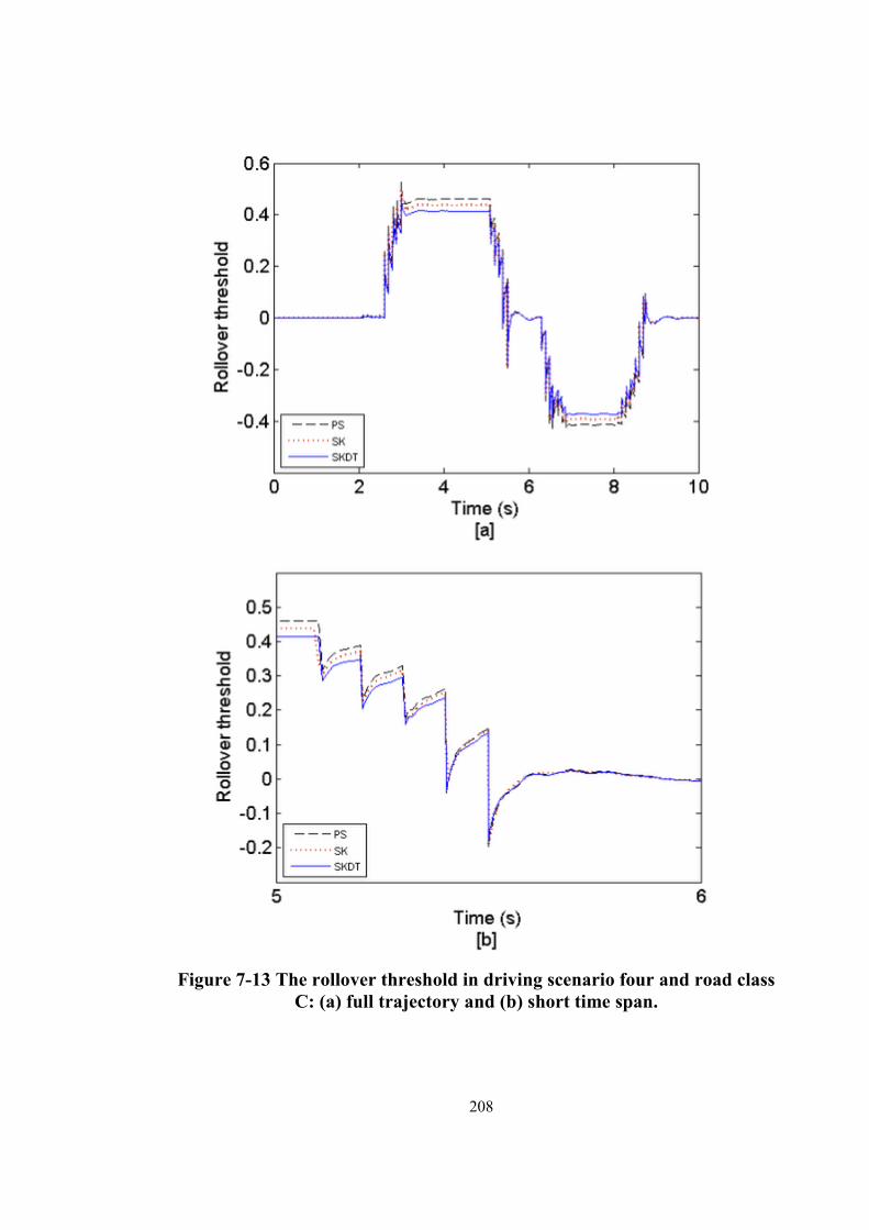
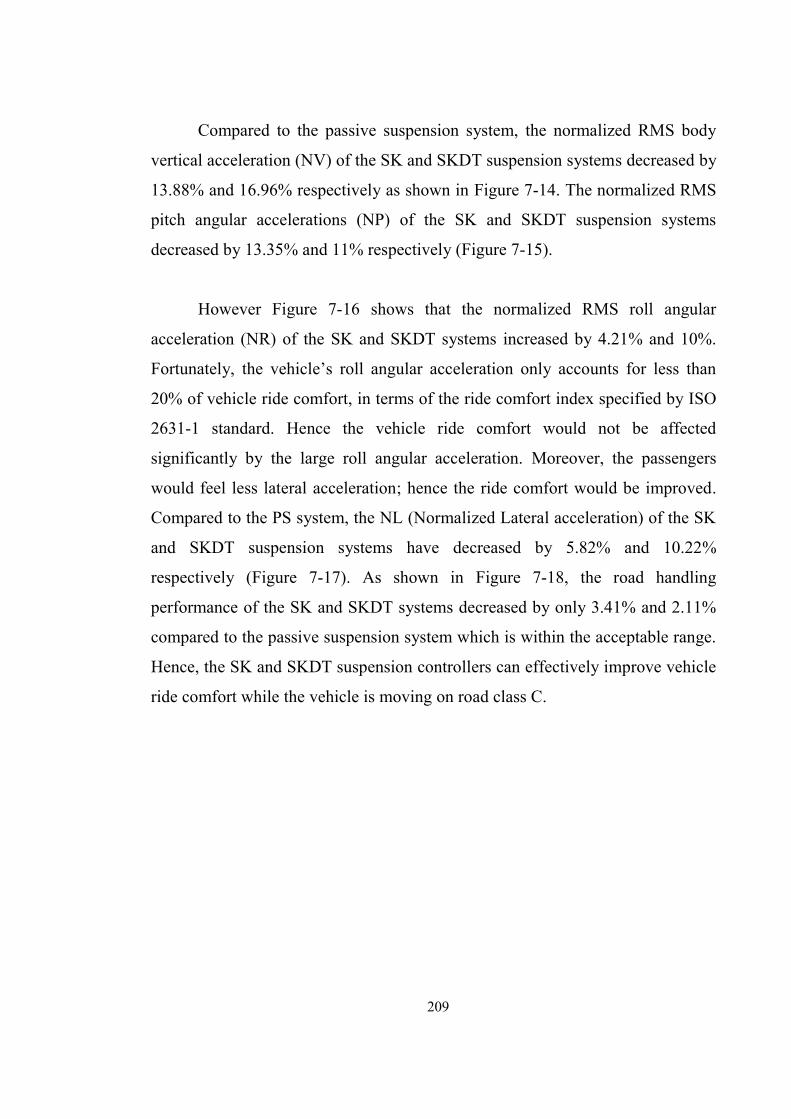
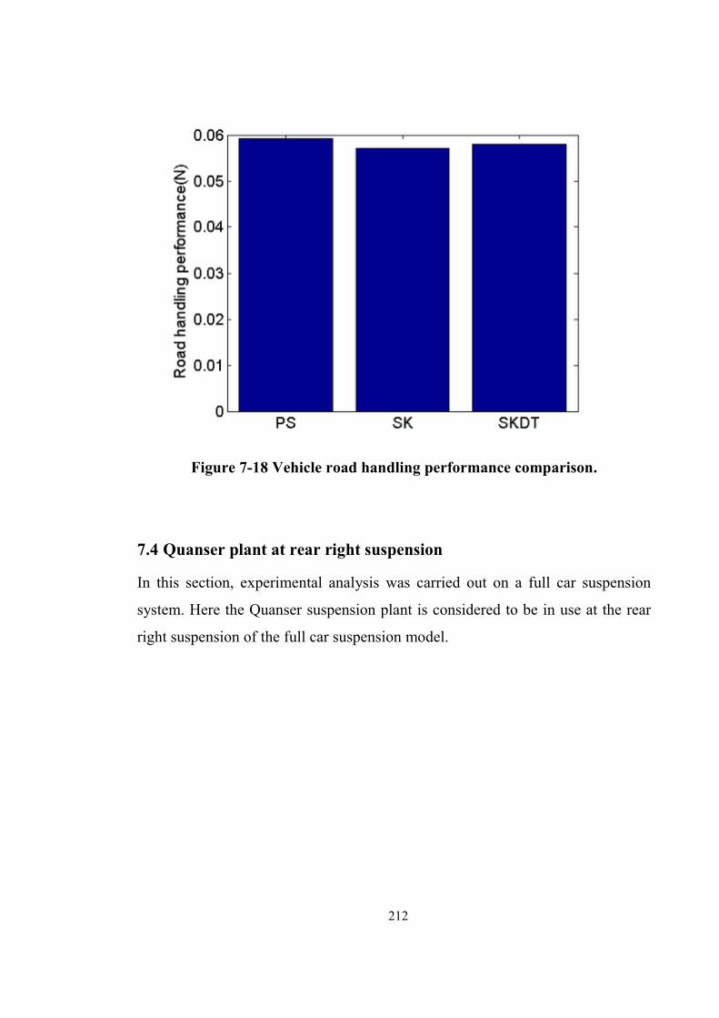
Figure 7-13 The rollover threshold in driving scenario four and road class C: (a) full trajectory and (b) short time span................................................................................208 Figure 7-14. Vehicle body vertical acceleration comparison. ....................................... 210
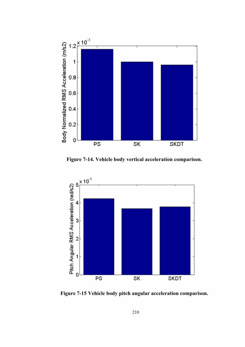
Figure 7-15 Vehicle body pitch angular acceleration comparison. .............................. 210
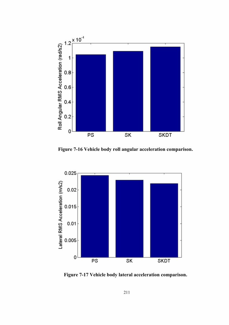
Figure 7-16 Vehicle body roll angular acceleration comparison. ................................. 211
Figure 7-17 Vehicle body lateral acceleration comparison. ......................................... 211
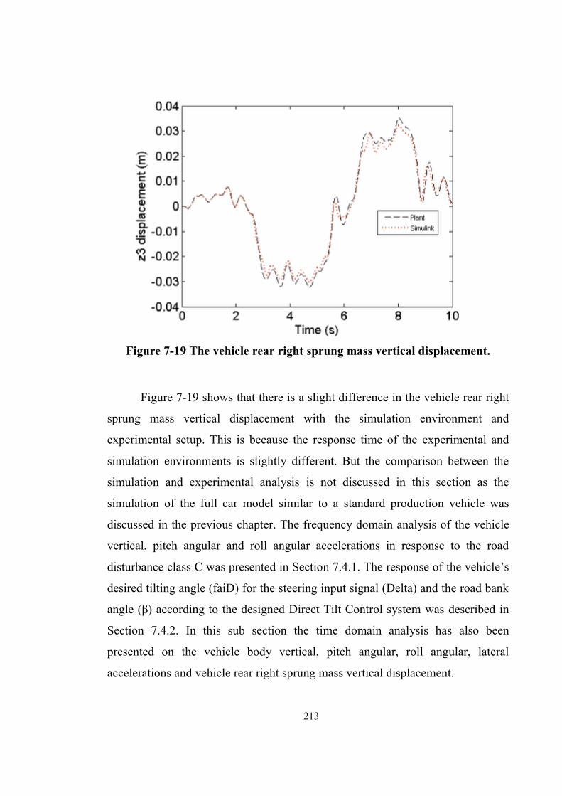
Figure 7-19 The vehicle rear right sprung mass vertical displacement. ....................... 213
Figure 7-20 The frequency response of vehicle body vertical acceleration: (a) at narrow frequency range and (b) at broad frequency range. .................................................... 215
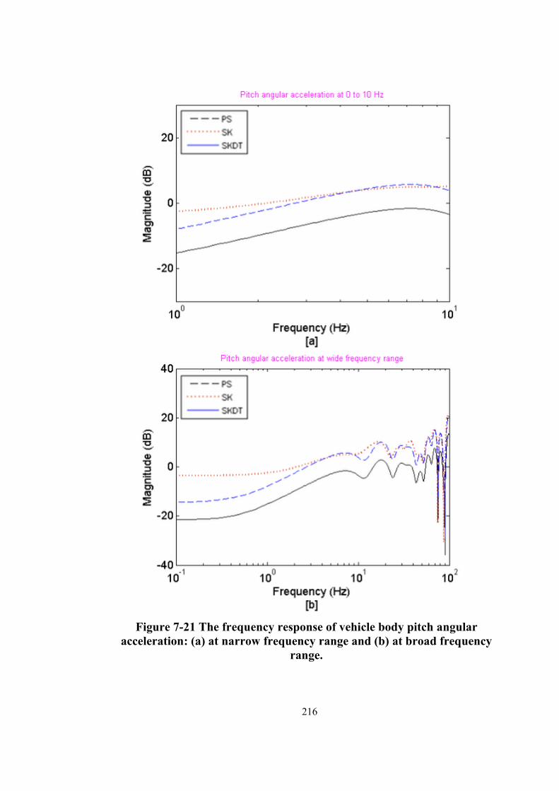
Figure 7-21 The frequency response of vehicle body pitch angular acceleration: (a) at narrow frequency range and (b) at broad frequency range. ........................................ 216
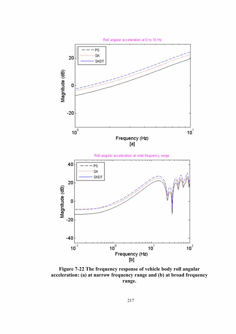
Figure 7-22 The frequency response of vehicle body roll angular acceleration: (a) at narrow frequency range and (b) at broad frequency range.........................................217 Figure 7-23 The response of steering and bank angle in driving scenario four and road class C: (a) Desired tilting angle (b) Required actuator force........................................218 Figure 7-24 The vehicle body vertical acceleration for driving scenario four and road class C: (a) full trajectory and (b) short time span.........................................................220 Figure 7-25 The pitch angular acceleration for driving scenario four and road class C: (a) full trajectory and (b) short time span. ......................................................................... 221
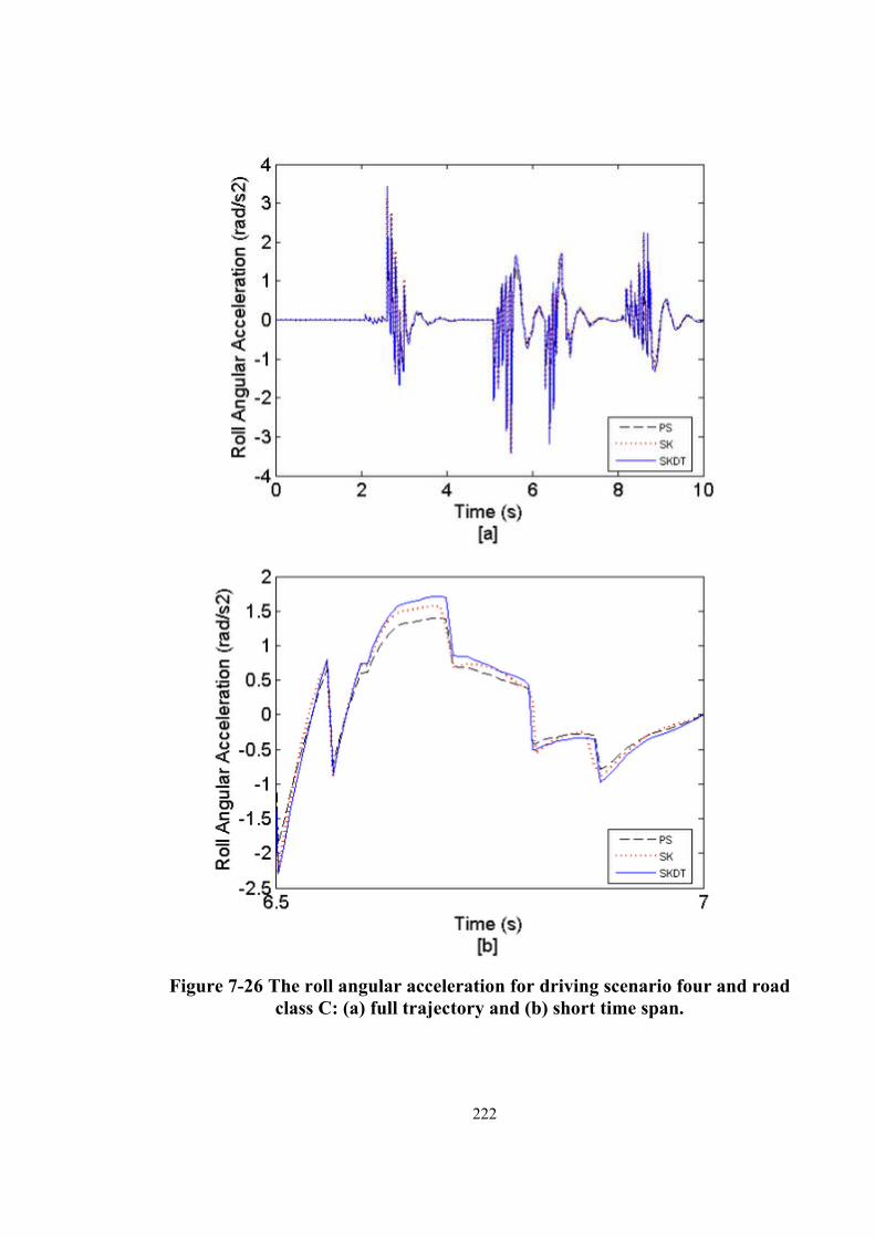
Figure 7-26 The roll angular acceleration for driving scenario four and road class C: (a) full trajectory and (b) short time span. ......................................................................... 222
Figure 7-27 The lateral acceleration for driving scenario four and road class C: (a) full trajectory and (b) short time span. ............................................................................... 223
Figure 7-28 The vehicle sprung mass m3‘s vertical displacement for driving scenario four and road class C: (a) full trajectory and (b) short time span. ............................... .224
xvi
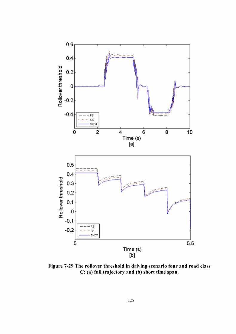
Figure 7-29 The rollover threshold in driving scenario four and road class C: (a) full trajectory and (b) short time span. ............................................................................... 225
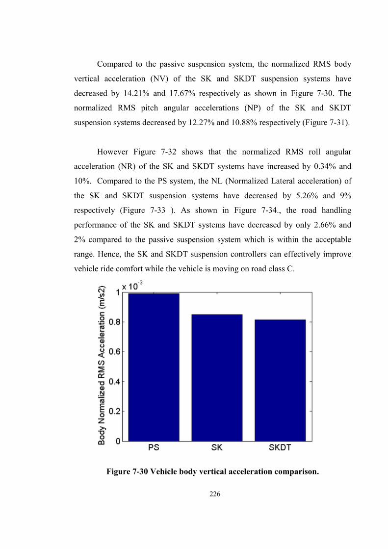
Figure 7-30 Vehicle body vertical acceleration comparison. ........................................ 226
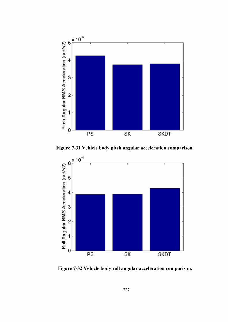
Figure 7-31 Vehicle body pitch angular acceleration comparison. .............................. 227
xvii
List of Tables Table 3-1 The parameters of quarter-car models ........................................................... 48
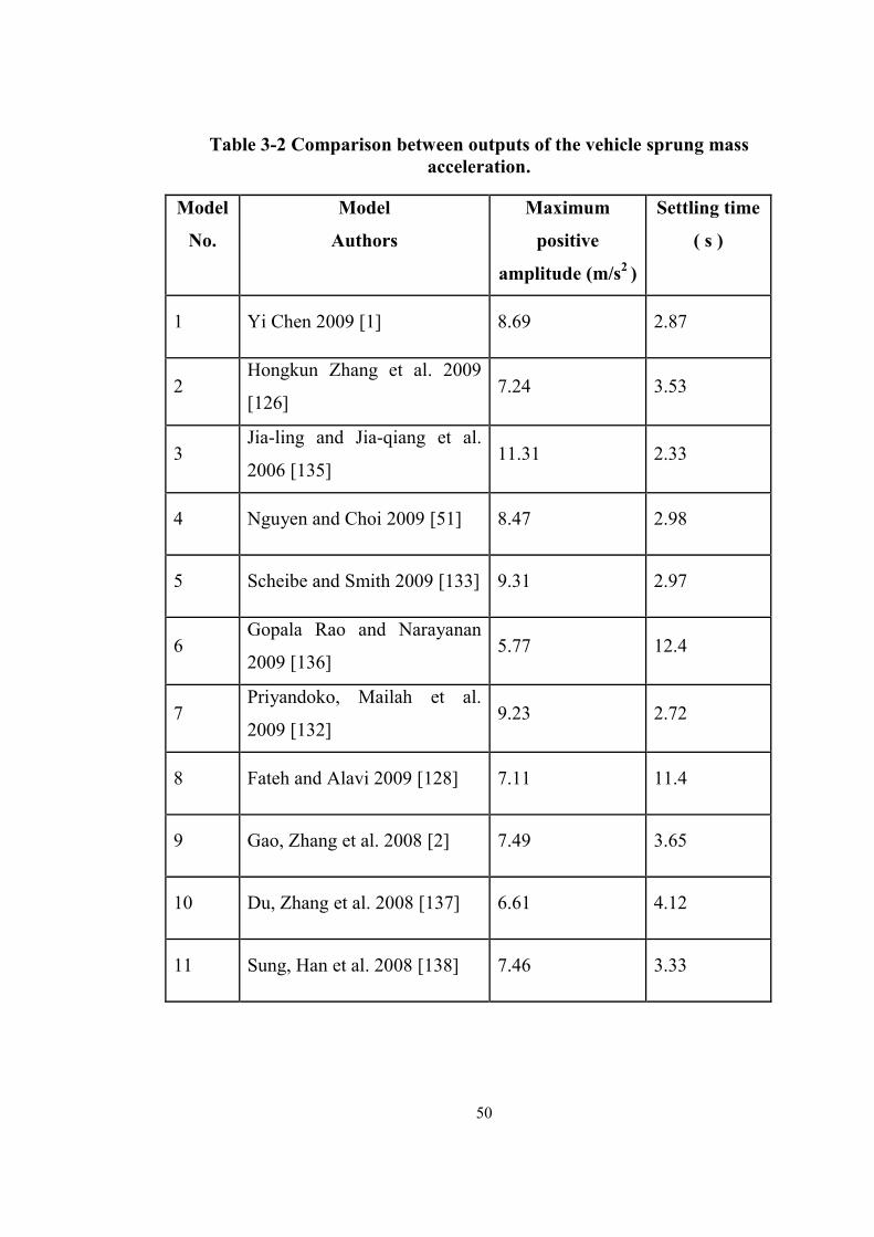
Table 3-2 Comparison between outputs of the vehicle sprung mass acceleration. ...... 50
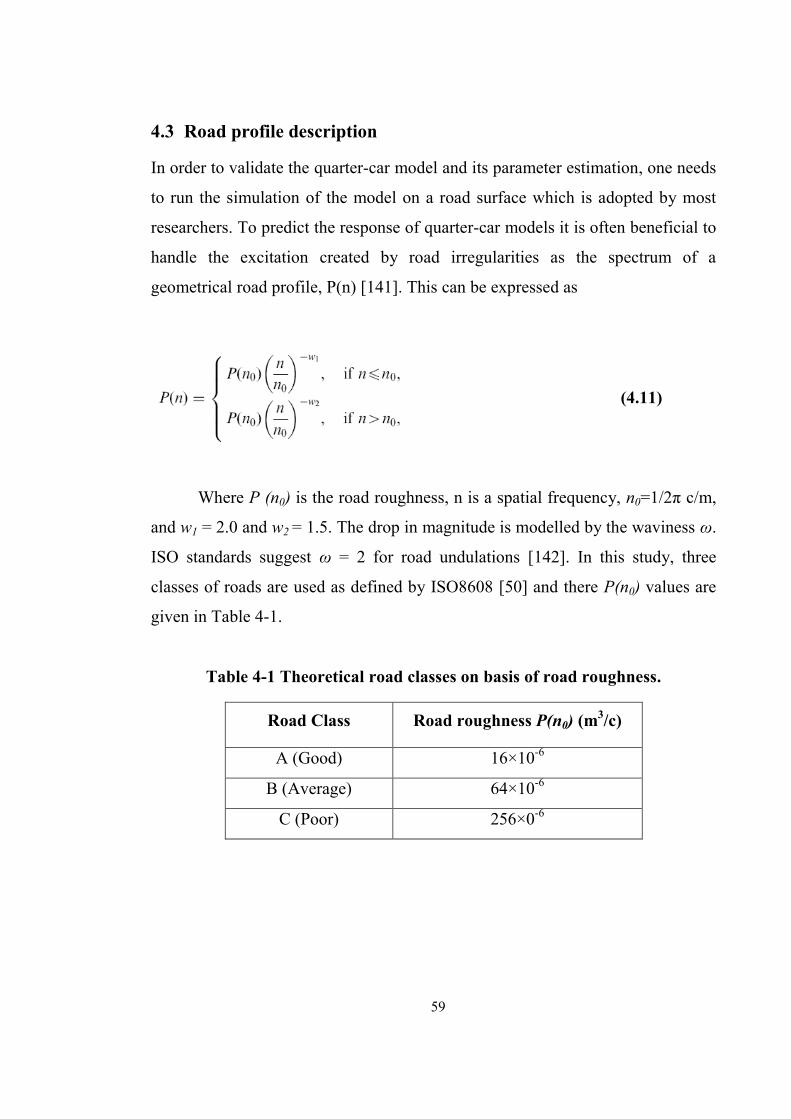
Table 4-1 Theoretical road classes on basis of road roughness. .................................... 59
Table 4-2 Nominal parameter values used in simulation. .............................................. 62
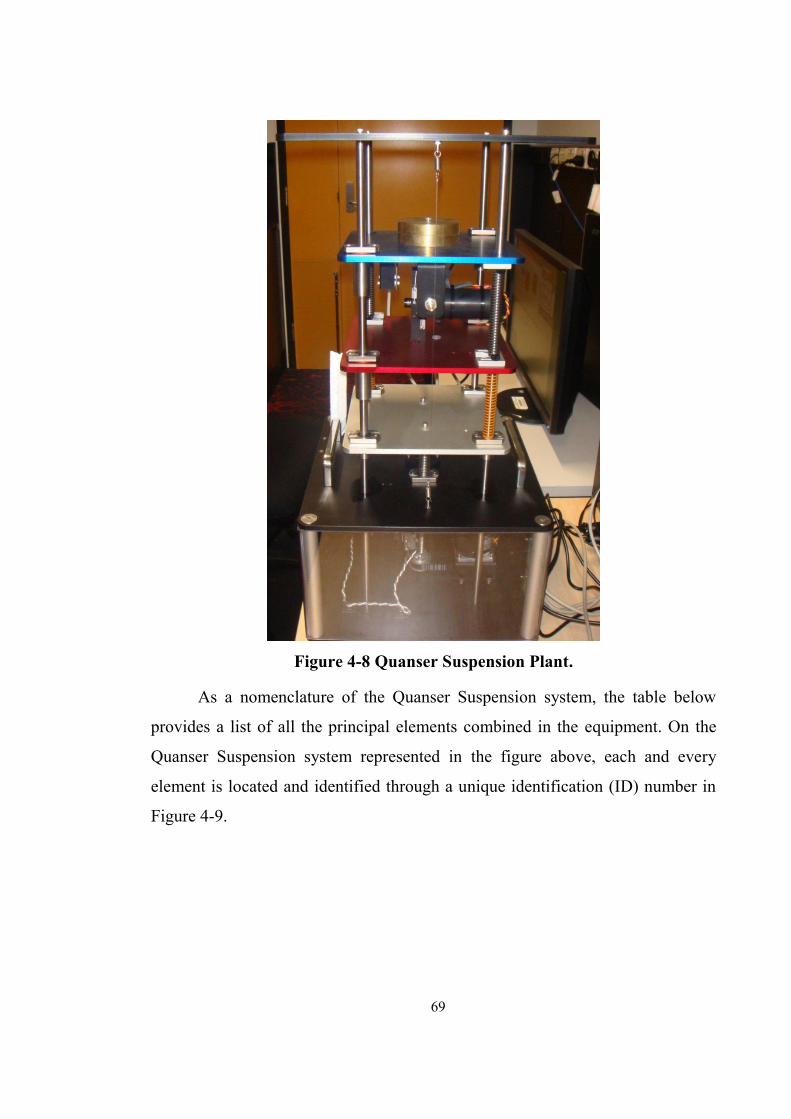
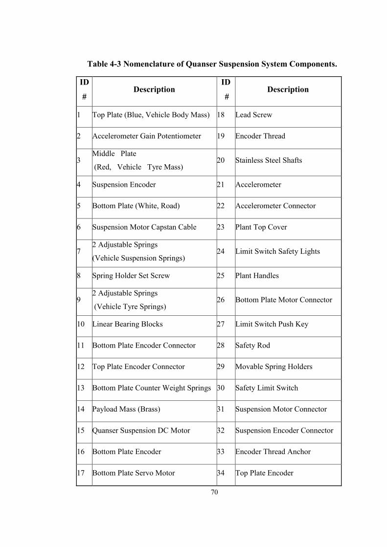
Table 4-3 Nomenclature of Quanser Suspension System Components. ........................ 70
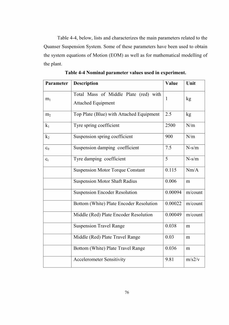
Table 4-4 Nominal parameter values used in experiment. ............................................ 76
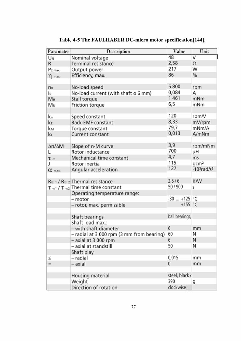
Table 4-5 The FAULHABER DC-micro motor specification[144]. .................................... 77
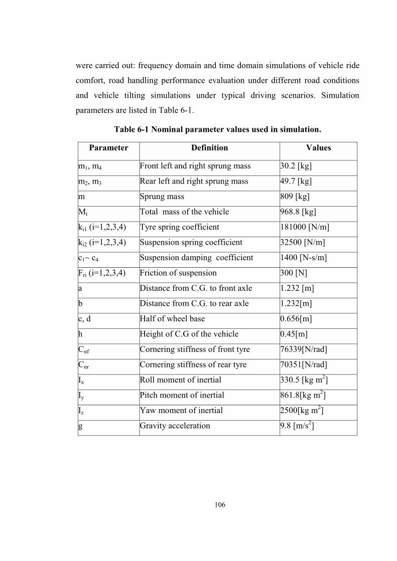
Table 6-1 Nominal parameter values used in simulation. ............................................ 106
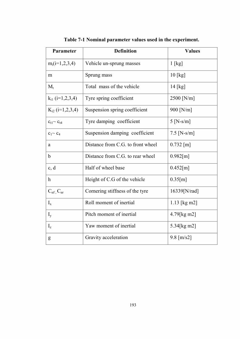
Table 7-1 Nominal parameter values used in the experiment. .................................... 193
1
Chapter 1 Introduction
1.1 Background
One of the most important considerations of the present automotive industry is to
provide passenger safety, through optimal ride comfort and road holding, for a
large variety of vehicle manoeuvres and road conditions. The comfort and safety
of the passenger travelling in a vehicle can be improved by minimizing the body
vibration, roll and heave of the vehicle body through an optimal road contact for
the tyres. The system in the vehicle that provides these actions is the vehicle
suspension, i.e., a complex system consisting of various arms, springs and
dampers that separate the vehicle body from the tyres and axles ( Figure 1-1and
Figure 1-2). In general, vehicles are equipped with fully passive suspension
systems due to their low cost and simple construction. The passive suspension
consists of springs, dampers and anti-roll bars with fixed characteristics. The
major drawback of the passive suspension design is that you cannot
simultaneously maximize both vehicle ride and handling performance. To
achieve better ride performance, a “soft” suspension needs to be introduced to
maintain contact between vehicle body and the tyre. The “soft” suspension easily
absorbs road disturbances. That is why most of the luxury cars employ “soft”
suspensions to provide a comfortable ride. The second characteristic of vehicle
performance is the road handling. This refers to a vehicle’s ability to maintain
contact between the vehicle’s tyre and the road during turns and other dynamic
manoeuvres. This can be achieved by “stiff” suspensions as seen in sports cars.
The challenge of the passive suspension system is in achieving the right
compromise between the two characteristics of vehicle performance which will
best suit the targeted consumer. However by introducing the active or semi-active
suspension system in the vehicle (Figure 1-3), a more desirable compromise can
be achieved between the benefits of the soft and stiff suspension system.
2
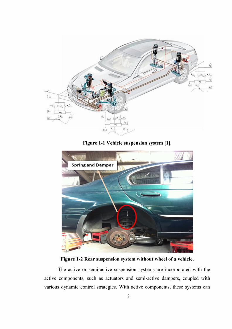
Figure 1-1 Vehicle suspension system [1].
Figure 1-2 Rear suspension system without wheel of a vehicle.
The active or semi-active suspension systems are incorporated with the
active components, such as actuators and semi-active dampers, coupled with
various dynamic control strategies. With active components, these systems can
3
provide adjustable spring stiffness and damping coefficients adapted to various
road conditions.
Since the early 1970s, many types of active and semi-active suspension
systems have been proposed to achieve better control of damping characteristics.
Although the active suspension system shows better performance in a wide
frequency range, its implementation complexity and cost prevents wider
commercial applications. That is why the semi-active suspension system has
been widely studied to achieve high levels of performance in terms of vehicle
suspension system. To control the damper of the semi-active suspension system,
many control strategies including Skyhook Surface Sliding Mode Control [1],
neural network control [2], H-infinity control [3], skyhook control, ground hook
control, Hybrid control [4],[5], fuzzy logic control [6],[7], neural network-based
fuzzy control [8], neuro-fuzzy control [9], discrete time fuzzy sliding mode
control [10], optimal fuzzy control [11] , adaptive fuzzy logic control [12], [13]
have been explored. Between all of the above control systems, the skyhook
control proposed by Karnopp et al. in 1974 [14] is widely used since it yields the
best compromise between vehicle performance and practical implementation of
semi-active suspension systems.
Figure 1-3 The Passive, Semi-active and Active suspension system.
4
In the past few decades researchers have modified the basic skyhook
control strategy by adding some variations and have named them optimal,
modified or adaptive type skyhook control strategies [15], [16]. But in most of
these studies, Skyhook Gain (SG) of the control strategy remains as a constant
value and it is usually chosen from a set of values as suited for the vehicle in the
simulation environment. One of the major goals of this research is to present a
new modified skyhook control strategy with adaptive SG.
This control strategy has also been employed on the full car model to
improve the isolation of the vibration and handling performance of the road
vehicle. The full car model designed in this research has nine degrees of freedom
and those are; the heave modes of four wheels and the heave, lateral, roll, pitch
and yaw modes of the vehicle body.
Nowadays, some researchers have focused on active steering control to
improve vehicle cornering [17-19]. Three types of active steering control
strategies have been proposed. These are the four wheel active steering system
(4WAS), the front wheel active steering system (FWAS) and the active rear
wheel steering system (RWAS). The four wheel active steering system (4WAS)
is the combination of the rear active steering system and the front active steering
system. In the FWAS system, the front wheel steer angle is determined by the
steering angle generated due to the driver’s direct steering input and a resultant
corrective steering angle input that is produced by the design of the active front
wheel steering controller.
Vehicle performance during cornering has been improved by most of the
car manufacturers by using electronic stability control (ESC). Car manufacturers
use different brand names for ESC, such as, Volvo named it DSTC (Dynamic
Stability and Traction Control); Mercedes and Holden called it ESP (Electronic
Stability Program); DSC (Dynamic Stability Control) is the term used by BMW
and Jaguar but despite the term used the processes are almost the same. To avoid
over steering and under steering during cornering, ESC extends the brake and
5
different torque on each wheel of the vehicle. But ESC reduces the longevity of
the tire as the tire skids while random braking. To overcome this problem a
vehicle can be tilted inwards via an active or semi-active suspension system.
The concept of ‘active tilting technology’ has become quite popular in
narrow tilting road vehicles and modern railway vehicles. Now in Europe, most
new high-speed trains are fitted with active tilt control systems and these trains
are used as regional express trains [20, 21]. To tilt the train inward during
cornering, tilting actuators are used as an element of the secondary active
suspension system. These actuators are named as bolsters. In a road vehicle
actuators are also used to affect the vehicle roll angle via an active suspension
system. Since the beginning of the 1950s, there has been extensive work done in
developing the Narrow Tilting Vehicle by both the automotive industry [22-25]
and academic researchers [26-30].
This particular small and narrow geometric property of the vehicle poses
stability problems when the vehicle needs to corner or change a lane. There are
also two types of control schemes that have been used to stabilize the narrow
tilting vehicle. These control schemes are defined as Direct Tilt Control (DTC)
and Steering Tilt Control (STC) systems as detailed in [27, 31, 32]. A typical
passenger vehicle body can be tilted up to 10° as the maximum suspension travel
is around 0.25 m. Then, the lateral acceleration of the tilted vehicle caused by
gravity can reach a maximum of about 0.17g [33]. Since the lateral acceleration
produced by normal steering manoeuvres is around 0.3–0.5 g, the active or semi-
active suspension systems have the potential of improving vehicle ride handling
performance [33]. Semi-active or active suspension systems can act promptly to
tilt the vehicle with the help of semi-active dampers or actuators. However, the
active suspension systems need to avoid over-sensitive reaction to driver’s
steering commands for vehicle safety. Recently Bose Corporation presented the
Bose suspension system [34] in which the high-bandwidth linear electromagnetic
dampers improved vehicle cornering. It is able to counter the body roll of the
6
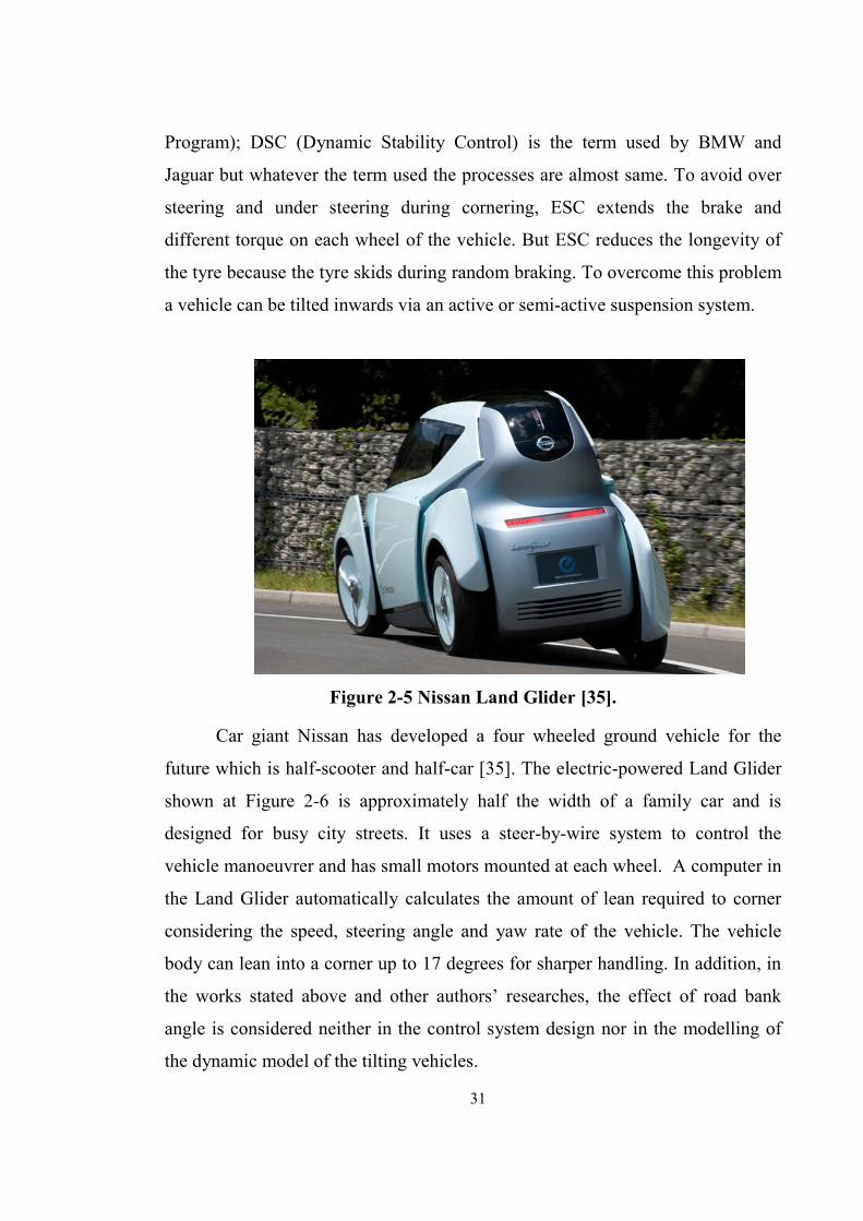
vehicle by stiffening the suspension while cornering. Car giant Nissan has
developed a four wheeled ground vehicle named Land Glider [35]. The vehicle
body can lean into a corner up to 17 degrees for sharper handling considering the
speed, steering angle and yaw rate of the vehicle. In addition, in the works stated
above and other research, the effect of road bank angle is neither considered in
the control system design nor in the dynamic model of the tilting standard
passenger vehicles [26, 27, 31, 32, 36-44]. Not incorporating the road bank angle
creates a non-zero steady state torque requirement. So this phenomena needs to
be addressed while designing the tilt control and the dynamic model of the full
car model. To lean a vehicle which incorporates the road bank angle, the
response time of the actuator or semi-active damper plays an important role.
The majority of the semi-active suspension systems use pneumatic or hydraulic
solutions as the actuator or semi-active damper [45-49]. These systems are
characterized by high force and power densities but suffer from low efficiencies
and response bandwidths. Commercial systems incorporating electromagnetic
elements (combine rotary actuators and mechanical elements) illustrate the
properties of the magneto-rheological fluids in damper technology to provide
adjustable spring stiffness. However, linear electromagnetic actuators appear as a
better solution for a semi-active suspension system in respect of their high force
densities, form factor and response bandwidth. The motivation and the
methodology of this research are described in the next section.
1.2 Research motivation and methodologies
The active suspension system has exploited superior performance in terms of
vehicle ride comfort and ride handling performances compared to other passive
and semi-active suspension systems in the automotive industry. Nevertheless,
they are not widely commercialized yet because of their high cost, weight,
complexity and energy consumption. Another major drawback of the active
suspension system is that it is not fail-safe in the situation of a power break-
7
down. That is why; the semi-active suspension system has been widely studied
and commercialized to achieve high levels of performance with ride comfort and
road handling. To control the damper of the semi-active suspension system,
many control strategies have been proposed but among all of them, skyhook
control proposed by Karnopp et al. in 1974 [14] is widely used since it yields the
best compromise between vehicle performance and practical implementation of
semi-active suspension systems. The skyhook control system has been adopted
and implemented to offer superior ride quality to commercial passenger vehicles.
However, this technology is still an emerging one, and elaboration and more
research work on different theoretical and practical aspects are required. In the
past few decades researchers have modified the basic skyhook control strategy by
adding some variations and naming them optimal, modified or adaptive type
skyhook control strategy [15] [16]. But in most of these studies, Skyhook Gain
(SG) of the control strategy remains as a constant value and it is usually chosen
from a set of values as suited for the vehicle in the simulation environment. One
of the major goals of this PhD research is to present a new modified skyhook
semi-active control strategy with adaptive skyhook gain.
According to this strategy, each wheel of the car behaves independently.
At first the road profile input has been captured for each wheel from the tyre
deflection measurements over a certain period of time. Then the quarter-car
model is simulated on board computer of the vehicle. It follows the new modified
skyhook control strategy with a range of SG. This method determines a certain
value of SG which is applied to the new modified skyhook control strategy to
dictate the semi-active suspension system of the corresponding car wheel.
Meanwhile the system behaves according to the modified skyhook control law
with an initial or previous value of the SG. After each period of time SG is
updated to match the road disturbance.
To evaluate the performance of the proposed closed loop feedback system,
a two degree of freedom quarter-car model has been used. The vibration isolation
8
and road handling performance of the proposed model has been analyzed and
compared with a passive system and three other skyhook controlled systems
subject to base excitation defined by ISO ISO8608 [50]. The other control
systems are the continuous skyhook control of Karnopp et al. [14], the modified
skyhook control of Bessinger et al. [15] and the optimal skyhook control of
Nguyen et al. [16]. An experimental evaluation of the proposed skyhook control
strategy has also been done by the Quanser Quarter-car Suspension plant. Then
the control strategy has been employed on the full car model to improve the
isolation of the vibration and handling performance of the road vehicle. The full
vehicle model designed in this research has nine degrees of freedom: the heave
modes of four wheels and the heave, lateral, roll, pitch and yaw modes of the
vehicle body.
Another major objective of this research is to improve the performance of
vehicles during cornering with little or no skidding using a new approach. That
approach tilts the standard passenger vehicle inward during cornering or sudden
lane change with consideration of the road bank angle, the steering angle, lateral
position acceleration, yaw rate and the velocity of the vehicle. The suspension
system considered here consists of linear electromagnetic damper (LEMD) in
parallel with the conventional mechanical spring and damper. This research has
two goals, firstly to find out the possibilities of tilting a car inwards through a
semi-active suspension system, and secondly to improve the vehicle ride comfort
and road handling performance. The stability control algorithm for tilting
vehicles has been designed in such a way that the driver does not need to have
special driving skills to operate the vehicle. In this research, the short comings of
existing direct tilt control systems are addressed. At first a dynamic model of a
tilting vehicle which considers the road bank angle is designed. Then an
improved direct tilt control system along with the modified skyhook control
system design is presented. This system takes into account the steering angle, the
road bank angle, lateral position acceleration, yaw rate and the velocity of the
9
vehicle. A yaw-rate sensor and a lateral acceleration sensor are placed at the
vehicle. The job of these sensors is to monitor the movement of the car body
along the vertical axis. The combined control system will do a comparative
analysis of the target value calculated and the actual value based on the driver's
input through the steering. Then control system will make a decision considering
the road bank angle, lateral position acceleration, yaw rate and velocity of the
vehicle. The moment the car begins to turn, the control system will intervene by
applying a precisely metered electromagnetic force using the separate linear
electromagnetic damper placed at each wheel. This lifts up the side of the
vehicle’s body opposite to the centre of the turn and turns down the side which is
on the same side of the turning point. This will make a certain angle between the
vehicle body and the road as directed by the controller. This angle, between the
road and the vehicle body, will move the vehicle’s centre of gravity towards the
turning point and will help the driver to turn smoothly using less road surface.
Moreover it will support the vehicle as it turns with more speed without skidding.
This research does not develop a new semi-active suspension physical model or a
linear electromagnetic damper. The application of semi-active suspension with
linear electromagnetic suspension system is suggested due to their reliability and
effectiveness over other technology and for practical implementation.
To achieve the research objectives, this thesis makes effective use of
different analysis methods, including MatLab/SIMULINK simulation processes;
and real-time tests and experiments where applicable. The next section outlines
the structure of the whole thesis.
1.3 Outline of the thesis
Following this introduction chapter, the remainder of the thesis is divided into
seven more chapters. Chapter 2 includes an extensive review of the literature on
different types of semi-active suspension control systems. Five widely known
control approaches are reviewed more deeply. Since the damper plays an
10
important role in the semi-active suspension system design, different types of
damper technologies are discussed including Quanser electromagnetic damper
which has been used in the experimental analysis of this research. Also described
is the tilting vehicle technology designed and developed by both the automotive
industry and academic researchers.
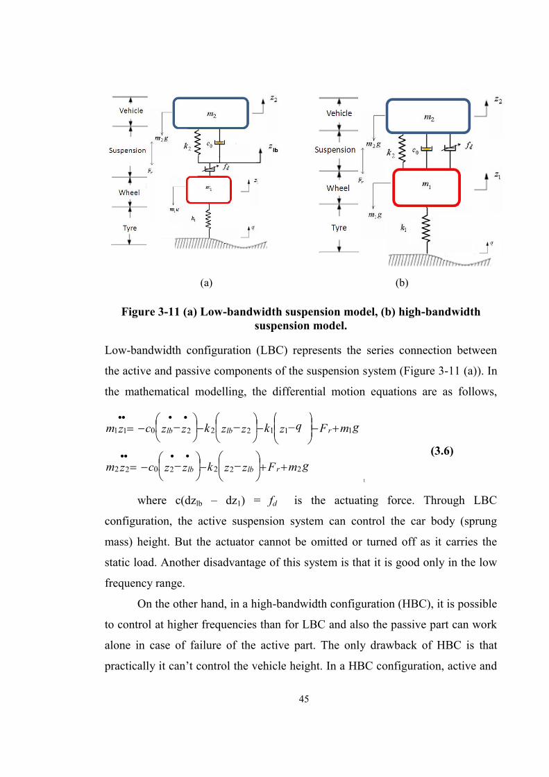
In Chapter 3, the vehicle suspension system is categorised and discussed
briefly. High and low bandwidth suspension system is also discussed. This
chapter also examines the uncertainties in modelling a quarter-car suspension
system caused by the effect of different sets of suspension parameters of a
corresponding mathematical model. From this investigation, a set of parameters
were chosen which showed a better performance than others in respect of peak
amplitude and settling time. These chosen parameters were then used to
investigate the performance of a new modified continuous skyhook control
strategy as set out in Chapter 4.
Chapter 4 consists of a brief discussion on the proposed modified skyhook
control approach, optimal skyhook control of Nguyen et al. [51], modified
skyhook control of Bessinger et al. [15] and continuous skyhook control of
Karnopp et al. [14]. A road profile was generated to study the performance of the
different controllers. The two degrees of freedom quarter-car model described in
Chapter 3 was simulated to compare the controller’s performances. Quanser
quarter-car suspension plant has been also used to compare the performance of
the controllers in the experimental environment. These models have also been
evaluated in terms of human vibration perception and admissible acceleration
levels based on ISO 2631 in this chapter.
Chapter 5 presents a methodology on how to integrate the proposed
skyhook control in a full car model to improve ride comfort and handling via a
semi-active suspension system. A technique to determine the vehicle rollover
propensity to avoid tipping over is also described. The road profile and four
driving scenarios are discussed in this chapter briefly which form a basis for the
11
analysis described in the next two chapters. A method to determine the
admissible acceleration level based on ISO 2631 is also discussed in this chapter.
The next chapter contains the simulation results of the semi-active suspension
system developed as described in this chapter.
In Chapter 6, the analysis of the simulation results of the dynamic model
of a full car model which considers the road bank angle is presented. The first
section describes the parameters of the full car that were used in the analysis
model and the environment of the simulation. The second section describes the
performance of the proposed skyhook control system under different road
conditions. In the third section the performance of the combined approach: the
proposed skyhook controller activated with the direct tilt control, is evaluated in
different driving scenarios. The next section is comprised of the summary of the
simulation while the vehicle is travelling on road class C and following driving
scenario four.
In Chapter 7, the analysis of the dynamics of a full car model is presented.
It incorporates the response of the Quanser quarter-car suspension plant as one of
the four wheels of the full car model. The performance of the combined approach
where the proposed skyhook controller is activated along with the direct tilt
control is evaluated in Sections 7.3 and 7.4 at frequency domain and time
domain.
Chapter 8 presents the overall conclusion of this Ph.D. thesis, followed by
future research recommendations.
12
Chapter 2 Literature review
2.1 Overview
In the literature available many robust and optimal control approaches or
algorithms were found in the design of automotive suspension systems. In this
chapter, some of these will be reviewed such as the linear time invariant H-
infinity control (LTIH), the linear parameter varying control (LPV) and model-
predictive controls (MPC). Five widely known control approaches, namely the
Linear quadratic regulator & Linear Quadratic Gaussian, sliding mode control,
Fuzzy and neuro-fuzzy control, sky-hook and ground-hook approaches are
reviewed more deeply. Since the damper plays an important role in the semi-
active suspension system design, different types of damper technologies are
discussed in the second section. This includes the Quanser electromagnetic
damper that was used in the experimental analysis in this research. Another
major objective of this research is to tilt the standard passenger vehicle inward
during cornering. So a brief literature review on automotive tilting technology is
included in the last section.
2.2 Control strategies
In general, a controlled system consists of a plant with sensors, actuators and a
control method is called a semi-active control strategy. A semi-active system is a
compromise between the active and passive systems. It offers some essential
advantages over the active suspension systems. The active control system
depends entirely on an external power source to control the actuators and supply
the control forces. In many active suspension applications this control approach
needs a large power source. On the other hand, semi-active devices need a lot
less energy than the active ones. Another critical issue of the active control
13
system is the stability robustness problem with respect to sensors or the whole
system failure; this issue becomes a big concern when centralized controllers are
employed in vehicle suspension design. The semi-active control device is similar
to the passive devices in which properties of the damper can be adjusted such
that spring stiffness and damping coefficient of the damper can be changed; thus,
they are robustly stable. That is why the semi-active suspension system is widely
used in the automotive industry.
Since Karnopp et al. [52] developed the Skyhook control strategy,
extensive research has been done in semi-active control strategies [1-4] [5, 6] [7-
11]. Most of this research has been done to find practical and easy
implementation methods or to achieve a higher level of vibration isolation, or
both. Adaptive-passive and semi-active vibration isolation is able to change the
suspension system properties, such as spring stiffness and damping rate of the
damper or actuator as a function of time. But the properties are changed
relatively slowly in an adaptive-passive suspension system. However in the semi-
active system, the suspension properties are able to change within a cycle of
vibration. The linear quadratic control is able to achieve both comfort and road
holding improvements through the semi-active or active suspension system. But
it requires the full state measurement or estimation which is difficult to achieve
[53][54]. Linear time invariant H-infinity control (LTIH) is able to provide
better results, improving both ride comfort and road handling ensuring pre-
defined frequency behaviour [54]. Due to the fixed weights, this control system
is limited to provide fixed performances [55, 56]. In 2006, Giorgetti et al. [57]
compared different semi-active control strategies based on optimal control. They
proposed a hybrid model with predictive optimal controller [54]. This control law
is implemented via a hybrid controller, which is able to switch between a large
numbers of controllers that depends on the function of the prediction horizon
[54]. It also requires a full state measurement which is difficult to achieve.
Recently, the uses of linear parameter varying (LPV) approaches have become
14
quite popular [54, 58, 59]. A LPV controller can either improve the robustness
considering the nonlinearities of the system or adapt the performances according
to measured signals of road displacement and suspension deflection [56, 60][54].
Another model-predictive control (MPC) system has been proposed by Canale et
al., in 2006 [61]. The MPC controller is able to provide good performances but it
requires an on-line fast optimization procedure [54]. As it involves optimal
control approach, a good knowledge of the model parameters and the full state
measurements are necessary to design the control system [62][54]. Choudhury et
al. [63] compared active and passive control strategies based on PID controller.
There are many semi-active control systems designed, implemented and tested by
many researchers. A few of them are described briefly in the following sub
sections.
2.2.1 Linear Quadratic Regulator & Linear Quadratic Gaussian
In the field of vehicle suspension control systems, the Linear Quadratic
Regulator (LQR) approach is a widely used and studied control system. It has
been studied and derived for a simple quarter-car model [64], half-vehicle models
[65] and also for a full vehicle [66]. An optimal result is possible to achieve
when tthe factors of the performance index such that acceleration of the body and
dynamic tyre load variation are taken into account. In the LQR approach, a state
estimator must be utilized if all the states are not available in the system, such as,
tyre deflections are difficult to measure in a moving vehicle. An estimator can
narrow the phase margin of the LQR suspension system to a great extent, but it
heightens the stability problems of the vehicle, especially if the suspension
system is a fully active system. To solve this problem, Doyle & Stein proposed
that the desired gain and phase properties can be obtained with a proper choice of
estimator gains [67]. When implementing the LQR system on a full vehicle,
another problem arises. The Riccati equation of the LQR system must be solved
numerically for a full vehicle model. The equation becomes very complex even
though the vehicle is assumed to be symmetrical and all the non-linear effects
15
created by the inertial effects and kinematical properties of the suspension system
are not included. Different types of numerical algorithms are proposed to solve
this issue but none of them could guarantee convergence and the stability of the
solution. The possibility of achieving a convergent solution decreases
significantly when the number of actuator decreases or the order of the control
system increases, or both, in a same system. [68].
The LQR approach has also the inability to take the changes in steady-
state into consideration. These changes are caused by the change of payload at
steady-state cornering of the vehicle. Elmadany & Abduljabbar [64], discussed a
method to overcome this problem. That method is integral control. The task of
integral control is to ensure the zero steady-state offset which would be applied
to a quarter-car model. For a full vehicle model, the integrator itself can
deteriorate the performance of the controller. The proper selection of the
integrator term and the gain of the integration time are a difficult problem in this
approach due to the external forces caused by the non-zero offset which vary
widely.
The optimal control method has been commonly used to accomplish a
better comfort or handling performance of a vehicle. Hrovat [69] has done
extensive research with half-car models, full-car models, one degree of freedom
models and two degree of freedom models. He minimized the cost functions of
the system combining excessive suspension stroke, sprung-mass jerk and sprung-
mass acceleration together using Linear Quadratic (LQ) optimal control.
Shisheie et al., [70] presented a novel algorithm based on the LQR
approach. It is able to optimally tune the PI controller’s gains of a first order plus
time delay system. In this approach, the cost function’s weighting matrices are
adjusted by damping ratio and the natural frequency of the closed loop system. In
1995 Prokop [71] used LQR and Linear Quadratic Gaussian (LQG) optimal
control theories utilizing road preview data or information to get better ride
16
quality. But the fact is, with respect to the system modelling errors, the LQG
controller is less robust and still today, determining the weighting coefficients for
the LQG is a very hard job. According to Shen [72], most of the weighting
coefficients for LQG/LQR control have been concluded by trial and error. Shen
also revealed that the renowned skyhook feedback strategy provides the best
outputs for the optimal feedback gain which reduces the mean square control
effort and the cost function of the sprung-mass’s mean square velocity.
2.2.2 Sliding mode control
In the last 20 years, sliding mode control (SMC) has become one of the most
active parts of control theory exploration. This exploration has established
successful applications in a variety of engineering control systems, for example,
aircrafts, automotive engines, suspension, electrical motors and robot
manipulators [73-75]. Shiri [76] has designed a sliding mode controller that is
robust to electric resistance changes and bounded mass and also able to reject
external disturbances. The simplicity system makes it adaptable to the
Electromagnetic Suspension System. The results of the simulation confirm the
robustness and the satisfactory performance of the designed controller against
uncertainties and disturbances. There has also been a considerable amount of
research done on the development of the theory of SMC problems for different
types of systems, such as, the fuzzy systems [77], the stochastic systems [78, 79]
and the uncertain systems [80].
In a real dynamical system, it is impossible to avoid uncertainties due to
the external disturbances and the modelling of the system. What is crucial is a
solution to the robust control problem for uncertain systems. SMC can be used to
deal with this problem. It is able to work with both uncertain linear and nonlinear
systems successfully in a unified frame work [81]. SMC design gives a
systematic approach to the problem of maintaining consistent performance and
17
stability in the face of the system’s modelling imprecision. Since the variable
structure with sliding mode (VSM) possesses the intrinsic nature of robustness,
the VSM is found to be an effective technique to control the systems with
uncertainties [82]. But the drawback of this system is; when the system reaches
the sliding mode state, the system with variable structure control becomes
insensitive to the variations of the plant parameters. Many different techniques to
design sliding mode controllers exist but the baselines of all the techniques are
very similar and can be divided into two main steps.
Firstly, design the control law of SMC in such a way that the trajectories
of the closed-loop motion of the system are directed towards the SMC sliding
surface and make an effort to keep the motion on the surface thereafter.
Secondly, develop the sliding surface in the state space in such a way that
the reduced-order sliding motion is able to satisfy the specifications specified by
the designers.
Utkin [82] introduced a novel PID type sliding mode control in which the
sliding mode starts at the initial instant. As a result, during the entire process, the
robustness of the system can be guaranteed. This system is also called an integral
sliding mode control (ISMC). Yagiz et al., [83] has proposed and developed a
sliding mode controller for a nonlinear vehicle model to overcome the problem
of fault diagnosis and tolerance. A modified SMC was designed by Chamseddine
et al., [84] for a linear full vehicle active suspension system with partial
knowledge of states of the system. For the conventional SMC strategy, the
desired dynamic state can only be achieved when the sliding mode occurs.
18
2.2.3 Fuzzy and neuro-fuzzy control
A vehicle suspension system is highly non-linear and very complicated.
Suspension actuation force changes when a vehicle rides on different road
conditions. Conventional control strategies are not able to adapt to different
environmental conditions. Fuzzy and neuro-fuzzy strategies can be used in
controlled suspension systems in many ways. Fuzzy Logic Control (FLC) is
appropriate for nonlinear systems. It can work with a complex system with no
precise math model. This is why; FLC is used in semi-active and active
suspension systems to control the disturbance rejection. FLC is able to be
insensitive to model and parameter inaccuracies with proper membership
functions and rule bases.
To calculate the desired damping coefficients for semi-active systems,
FLC can be utilized directly according to Al-Holou & Shaout [85]. Al-Holou &
Shaout compared FLC to both a passive and sky-hook controllers. The authors
employed FLC to the semi-active actuator to calculate the desired damping
coefficient. In this study, a wide range of semi-active actuators were used. An
important finding of this research was that most of the FLC systems show similar
results to the sky-hook control system. It has been found that compared to the
sky-hook control system, a fuzzy controlled semi-active suspension system
showed slightly smaller RMS-values of the body acceleration. Al-Holou &
Shaout also showed that the semi-active suspension system with FLC increased
the variation of dynamic tyre contact force compared to the skyhook controlled
semi-active suspension system.
FLC can also be used to calculate the required force for the active
suspension system [86]. Barr & Ray compared the fuzzy-controlled active system
with both the passive suspension system and the LQR active suspension systems.
The authors have shown that the ride handling characteristic (the variation of
19
dynamic tyre load) of FLC is better than the LQR and the passive suspension
system. This result is slightly surprising, at least in the LQR active suspension
system case. Moreover, the LQR-regulator cost function was not presented in this
research.
On the other hand, Neural Networks consists of a variety of alternative
features such as computation, distributed representation, massive parallelism,
adaptability, generalization ability, and inherent contextual information
processing. They can be utilized to model different types of ambiguities and
uncertainties, which are often experienced in real life. Zhang et al., [87]
presented a multi-body vehicle dynamics model using ADAMS and a multilayer
feed forward neural network of a series parallel structure. The weights and
threshold of neural networks have been optimized in this research. The result of
the combine simulation of MatLab and ADAMS shows that the network
convergence took place rapidly and the maximum error of identification is less
than 0.05%. The authors claimed that the designed genetic neural network can
avoid the difficulty of establishing accurately mathematical model for the vehicle
semi-active suspension system.
The main objective of the hybridization of the control systems (using
neural networks and fuzzy logic) is to overcome the weaknesses in one
technology by using the strengths of the other during its application with
appropriate integration. In the majority of the studies concerning neural networks
and fuzzy logic, the force of the actuator of the active suspension system or the
damping coefficient of the semi-active suspension system is not controlled
directly. Choi et al. [9] proposed a combination of neuro-fuzzy control approach
to dictate a military tracked vehicle semi-active suspension system. The
fuzzification phase of the presented controller was continuously modified
through a neural network. In this study, the models of real existing electro-
20
rheological semi-active actuator units and a 16-degree of freedom vehicle model
were utilized. For Direct Current Motor speed control on line, Youssef et al. [88]
have proposed an adaptive particle swarm optimization method for adapting the
weights of fuzzy neural networks. An adaptive neuro-fuzzy control has been
introduced by Khalid et al., [89] on the basis of particle swarm optimization
tuned subtractive clustering to provide critical information about the presence or
absence of a fault in a two tank process. Kashani & Strelow derived [90] a
control system which consists of multiple Linear Quadratic Gaussian controllers
around different operating points of the suspension system, and blended the
desired control actions of each controller with a fuzzy-logic mixed algorithm.
FLC was utilized to prevent the suspension from bottoming in this study.
Kashani & Strelow claimed that this type of blending of controller action is a
fruitful idea and able to improve the vehicle suspension system. But the
limitations of practical implementation; such as maximum free rattle space can
be taken into account with decision logic of fuzzy logic control.
2.2.4 Skyhook control method
The Skyhook control is an effective vibration control algorithm which is able to
dissipate the energy of the system at a high rate. For more than three decades, the
skyhook control strategy has been widely researched. In 1974, Karnopp et al.
[14] introduced the skyhook control strategy which is still used frequently in
vehicle suspension applications. The name ‘‘skyhook’’ originates from the idea
where a passive damper is imagined to be hooked from an imaginary inertial
reference point or the sky. Skyhook damping is a damping force that is in the
opposite direction to the sprung-mass absolute velocity and is proportional to the
absolute velocity of the sprung-mass.
21
Figure 2-1. An ideal skyhook configuration.
The above figure shows an ideal configuration of the skyhook semi-active
control which has a sprung mass hooked by a damper with skyhook damping
constant from an imaginary sky (fixed ceiling); hence the name “skyhook”
was used. If the damping force of the skyhook damper is then the ideal
skyhook control law can be expressed as:
(2.1)
Here, xs is the displacement. The skyhook controlled semi-active
suspension system (damper) utilizes a small amount of energy to run a valve,
which adjusts the damping force. The damper valve can be a fluid valve or a
mechanical element if it is a mechanically adjustable damper. In a
magnetorheological (MR) damper, the behaviour of rheological fluid changes
according to the designed control system.
The active continuous skyhook control policy can also be ideally realized
using an actuator or active force generator. Karnopp et al. [14] proposed the
skyhook having a two-state control scheme named an ON-OFF control system.
This control strategy switches between high and low damping states in order to
achieve body comfort specifications [54]. But this control policy offers the
ms
22
damping force as equal to zero when the direction of sprung mass velocity and
the relative velocity of the sprung mass with respect to un-sprung mass or ground
is opposite. But in practice applying zero damping force is not practicable for any
semi-active damper. In 1974 Karnopp et al. [14] realized the complexity of the
skyhook ON-OFF control method when it claims the force is need to be equal to
zero. However because of the simplicity and practical implementation of the
skyhook ON-OFF control strategy, it is widely used for vehicle suspension
control [91]. In 1983, Karnopp [92] also proposed a new approach for a semi-
active control system which consists of a variable stiffness method. In this
control scheme the damper is in a series connection with a spring of high
stiffness and the author suggested changing the stiffness of the spring according
to the change in the damping coefficient of the damper.
Ahmadian and Vahdati [5] revealed that much research has been done on
other variations of the skyhook control strategy in the past two decades, such as,
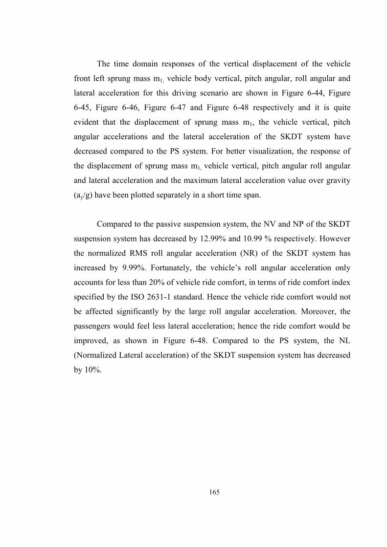
The time domain responses of the vertical displacement of the vehicle
front left sprung mass m1, vehicle body vertical, pitch angular, roll angular and
lateral acceleration for this driving scenario are shown in Figure 6-44, Figure
6-45, Figure 6-46, Figure 6-47 and Figure 6-48 respectively and it is quite
evident that the displacement of sprung mass m1, the vehicle vertical, pitch
angular accelerations and the lateral acceleration of the SKDT system have
decreased compared to the PS system. For better visualization, the response of
the displacement of sprung mass m1, vehicle vertical, pitch angular roll angular
and lateral acceleration and the maximum lateral acceleration value over gravity
(ay/g) have been plotted separately in a short time span.
Compared to the passive suspension system, the NV and NP of the SKDT
suspension system has decreased by 12.99% and 10.99 % respectively. However
the normalized RMS roll angular acceleration (NR) of the SKDT system has
increased by 9.99%. Fortunately, the vehicle’s roll angular acceleration only
accounts for less than 20% of vehicle ride comfort, in terms of ride comfort index
specified by the ISO 2631-1 standard. Hence the vehicle ride comfort would not
be affected significantly by the large roll angular acceleration. Moreover, the
passengers would feel less lateral acceleration; hence the ride comfort would be
improved, as shown in Figure 6-48. Compared to the PS system, the NL
(Normalized Lateral acceleration) of the SKDT suspension system has decreased
by 10%.
166
Figure 6-44 The vehicle sprung mass m1‘s vertical displacement for driving
scenario four: (a) full trajectory and (b) short time span.
167
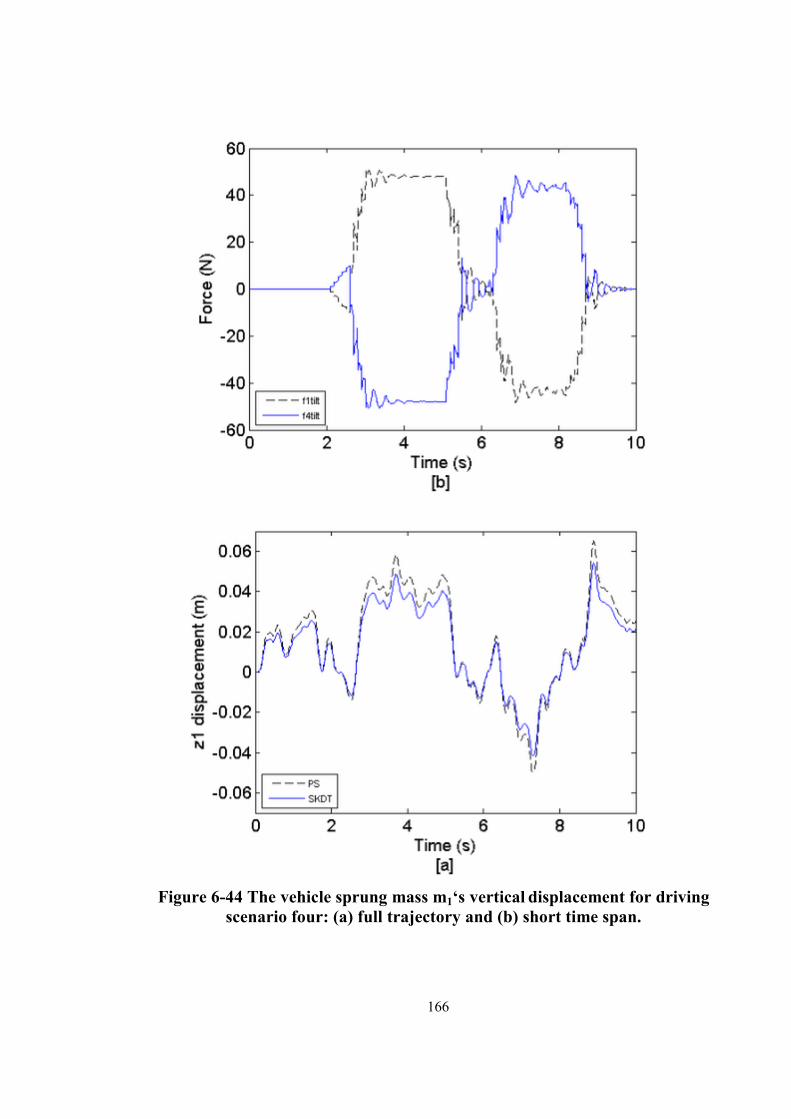
Figure 6-45 The vehicle body vertical acceleration for driving scenario four:
(a) full trajectory and (b) short time span.
168
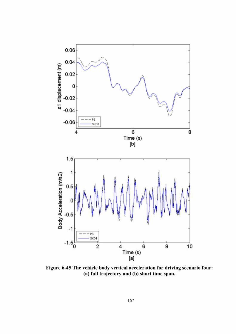
Figure 6-46 The pitch angular acceleration for driving scenario four: (a) full
trajectory and (b) short time span.
169
Figure 6-47 The roll angular acceleration for driving scenario four: (a) full
trajectory and (b) short time span.
170
Figure 6-48 The lateral acceleration for driving scenario four: (a) full trajectory and (b) short time span.
171
Figure 6-49 The rollover threshold in driving scenario four: (a) full trajectory and (b) short time span.
172
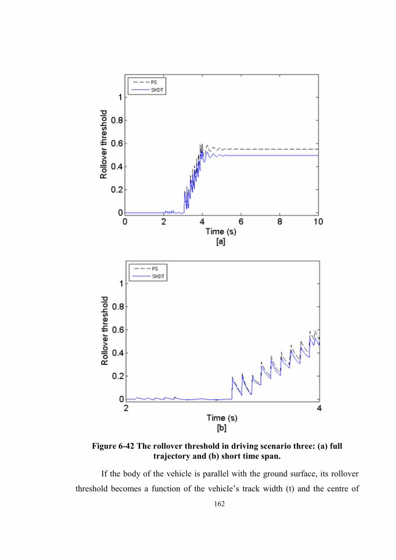
If the body of the vehicle is parallel with the ground surface, its rollover
threshold becomes a function of the vehicle’s track width (t) and the centre of
gravity height (h) as depicted in equation (5.17). The maximum allowable
rollover threshold of this vehicle is 1.45. The rollover threshold defines the
maximum lateral acceleration value over gravity (ay/g) that the vehicle would be
able to reach before tipping over. From Figure 6-49 (a) and (b), it is apparent that
(ay/g) never exceeds the maximum allowable rollover threshold of this vehicle.
Hence the vehicle remains stable throughout the trajectory of this driving
scenario.
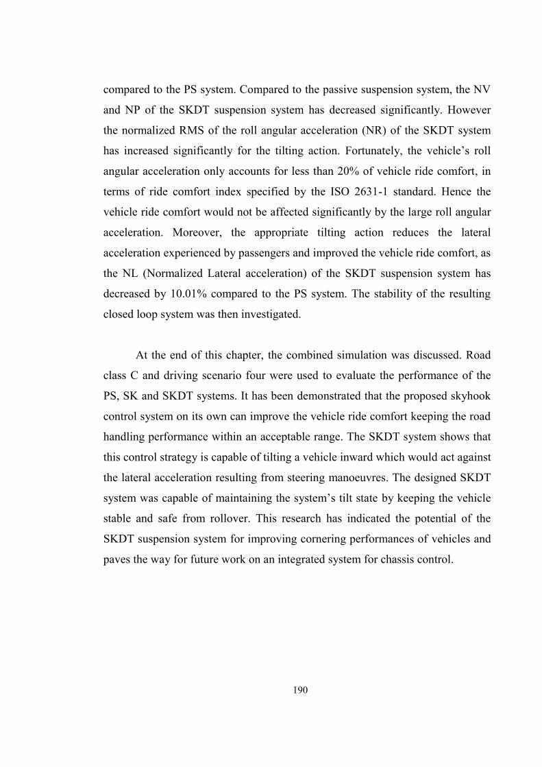
However the road handling performance of the skyhook controlled
suspension system has decreased by only 2% compared to the passive suspension
system. But the SKDT system’s weighted RMS acceleration value of the sprung
mass obtained in this simulation is 0.72 which is within the acceptable range.
6.5 Simulation Summary
The objective of this section is to summarize the evaluation of the SK system
(the proposed skyhook suspension system) and the SKDT system where the
direct tilt control is activated along with the proposed skyhook controller in the
same simulation. The performance of the SK and SKDT systems are compared to
the PS system (the passive suspension system). In this simulation, the vehicle
experienced road class C defined by ISO8608 described in Section 5.5. The
vehicle trajectory defined by the driving scenario four (Section 5.5). This driving
scenario has been used as if the vehicle experienced both left and right turns. The
frequency and time domain analysis are presented separately in the following
sections.
173
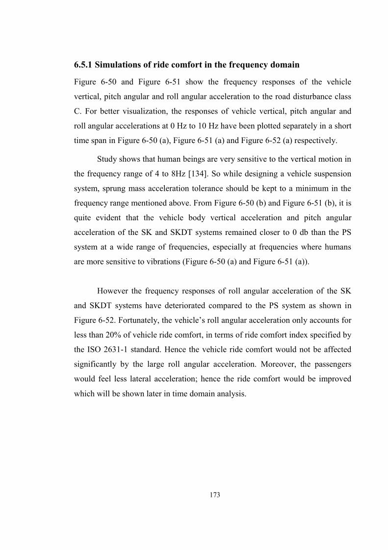
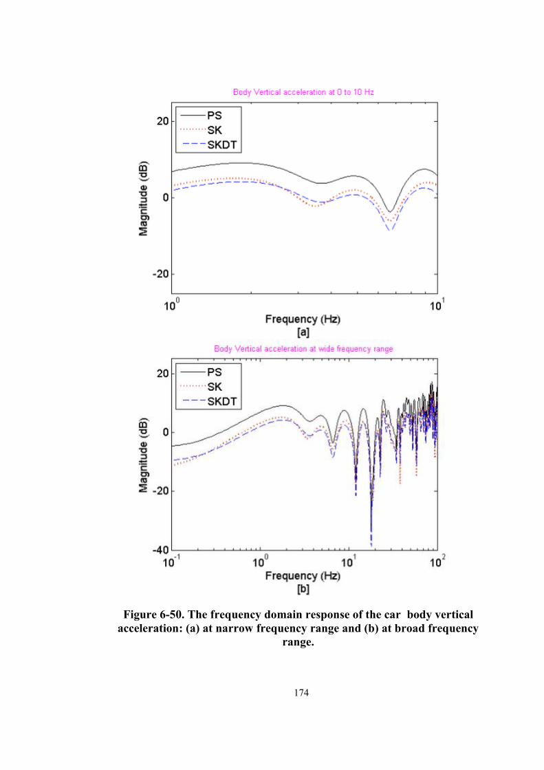
6.5.1 Simulations of ride comfort in the frequency domain
Figure 6-50 and Figure 6-51 show the frequency responses of the vehicle
vertical, pitch angular and roll angular acceleration to the road disturbance class
C. For better visualization, the responses of vehicle vertical, pitch angular and
roll angular accelerations at 0 Hz to 10 Hz have been plotted separately in a short
time span in Figure 6-50 (a), Figure 6-51 (a) and Figure 6-52 (a) respectively.
Study shows that human beings are very sensitive to the vertical motion in
the frequency range of 4 to 8Hz [134]. So while designing a vehicle suspension
system, sprung mass acceleration tolerance should be kept to a minimum in the
frequency range mentioned above. From Figure 6-50 (b) and Figure 6-51 (b), it is
quite evident that the vehicle body vertical acceleration and pitch angular
acceleration of the SK and SKDT systems remained closer to 0 db than the PS
system at a wide range of frequencies, especially at frequencies where humans
are more sensitive to vibrations (Figure 6-50 (a) and Figure 6-51 (a)).
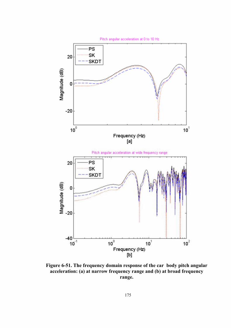
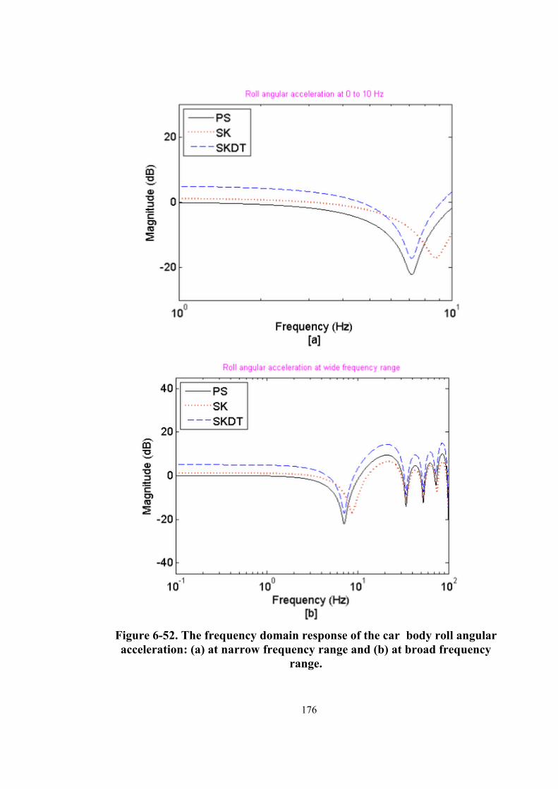
However the frequency responses of roll angular acceleration of the SK
and SKDT systems have deteriorated compared to the PS system as shown in
Figure 6-52. Fortunately, the vehicle’s roll angular acceleration only accounts for
less than 20% of vehicle ride comfort, in terms of ride comfort index specified by
the ISO 2631-1 standard. Hence the vehicle ride comfort would not be affected
significantly by the large roll angular acceleration. Moreover, the passengers
would feel less lateral acceleration; hence the ride comfort would be improved
which will be shown later in time domain analysis.
174
Figure 6-50. The frequency domain response of the car body vertical acceleration: (a) at narrow frequency range and (b) at broad frequency
range.
175
Figure 6-51. The frequency domain response of the car body pitch angular acceleration: (a) at narrow frequency range and (b) at broad frequency
range.
176
Figure 6-52. The frequency domain response of the car body roll angular acceleration: (a) at narrow frequency range and (b) at broad frequency
range.
177
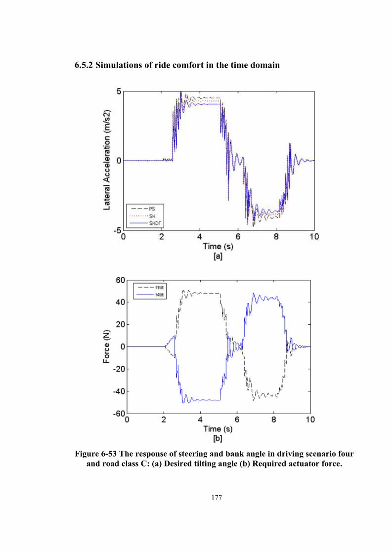
6.5.2 Simulations of ride comfort in the time domain
Figure 6-53 The response of steering and bank angle in driving scenario four
and road class C: (a) Desired tilting angle (b) Required actuator force.
178
In this section, vehicle reaction to the driving scenario using the PS and the
SKDT semi-active suspension system is described. Figure 6-53(a) shows the
response of the vehicle’s desired tilting angle (faiD) for the steering input signal
(Delta) and the road bank angle (β) according to the designed Direct Tilt Control
(Section 5.4.1). The required actuator force to tilt the vehicle according to the
desired tilting angle is depicted in Figure 6-53(b).
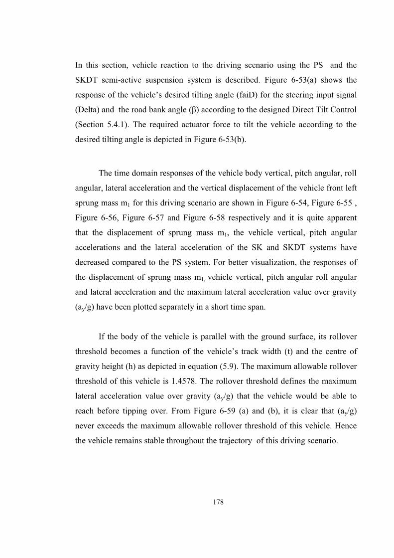
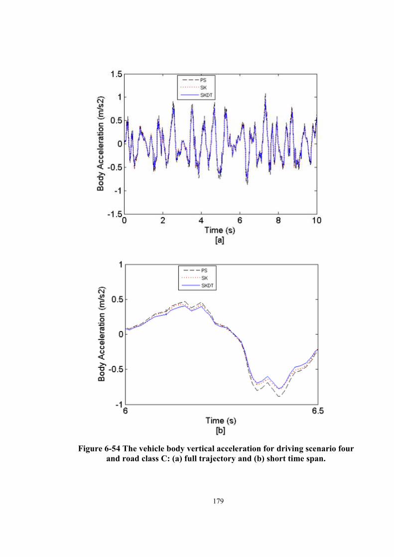
The time domain responses of the vehicle body vertical, pitch angular, roll
angular, lateral acceleration and the vertical displacement of the vehicle front left
sprung mass m1 for this driving scenario are shown in Figure 6-54, Figure 6-55 ,
Figure 6-56, Figure 6-57 and Figure 6-58 respectively and it is quite apparent
that the displacement of sprung mass m1, the vehicle vertical, pitch angular
accelerations and the lateral acceleration of the SK and SKDT systems have
decreased compared to the PS system. For better visualization, the responses of
the displacement of sprung mass m1, vehicle vertical, pitch angular roll angular
and lateral acceleration and the maximum lateral acceleration value over gravity
(ay/g) have been plotted separately in a short time span.
If the body of the vehicle is parallel with the ground surface, its rollover
threshold becomes a function of the vehicle’s track width (t) and the centre of
gravity height (h) as depicted in equation (5.9). The maximum allowable rollover
threshold of this vehicle is 1.4578. The rollover threshold defines the maximum
lateral acceleration value over gravity (ay/g) that the vehicle would be able to
reach before tipping over. From Figure 6-59 (a) and (b), it is clear that (ay/g)
never exceeds the maximum allowable rollover threshold of this vehicle. Hence
the vehicle remains stable throughout the trajectory of this driving scenario.
179
Figure 6-54 The vehicle body vertical acceleration for driving scenario four and road class C: (a) full trajectory and (b) short time span.
180
Figure 6-55 The pitch angular acceleration for driving scenario four and road class C: (a) full trajectory and (b) short time span.
181
Figure 6-56 The roll angular acceleration for driving scenario four and road class C: (a) full trajectory and (b) short time span.
182
Figure 6-57 The lateral acceleration for driving scenario four and road class C: (a) full trajectory and (b) short time span.
183
Figure 6-58 The vehicle sprung mass m1‘s vertical displacement for driving scenario four and road class C: (a) full trajectory and (b) short time span.
184
Figure 6-59 The rollover threshold in driving scenario four and road class C: (a) full trajectory and (b) short time span.
185
Compared to the passive suspension system, the normalized RMS body
vertical acceleration (NV) of the SK and SKDT suspension systems have
decreased by 10.68% and 12.99% respectively as shown in Figure 6-60. The
normalized RMS pitch angular accelerations (NP) of the SK and SKDT
suspension systems have decreased by 9.29% and 10.99% respectively (Figure
6-61).
However Figure 6-62 shows that the normalized RMS roll angular
acceleration (NR) of the SK and SKDT systems have increased by 0.61% and
9.99%. Fortunately, the vehicle’s roll angular acceleration only accounts for less
than 20% of vehicle ride comfort, in terms of ride comfort index specified by the
ISO 2631-1 standard. Hence the vehicle ride comfort would not be affected
significantly by the large roll angular acceleration. Moreover, the passengers
would feel less lateral acceleration; hence the ride comfort would be improved.
Compared to the PS system, the NL (Normalized Lateral acceleration) of the SK
and SKDT suspension systems have decreased by 0.46% and 10% respectively
(Figure 6-63).
As shown in Figure 6-64, the road handling performance of the SK and
SKDT systems have decreased by only 2.09% and 2% compared to the passive
suspension system. But the weighted RMS acceleration value of the sprung mass
obtained in this simulation is 0.65 and 0.72 for the SK and SKDT systems
respectively which are within the acceptable range of international code ISO
2631 [143]. Hence, the SK and SKDT suspension systems are able to improve
ride comfort of the vehicle effectively while the vehicle is moving on road class
C.
186
Figure 6-60 Vehicle body vertical acceleration comparison.
Figure 6-61 Vehicle body pitch angular acceleration comparison.
187
Figure 6-62 Vehicle body roll angular acceleration comparison.
Figure 6-63.Vehicle body lateral acceleration comparison.
This chapter describes the conclusion reached from the analysis of the
simulations that were carried out to investigate the proposed skyhook control
suspension system and the designed Direct Tilt Control system. The SK and
SKDT systems were applied to the dynamic model of a full car which considers
the road bank angle. At first, the responses of the dynamic model of the full car
on different road classes A, B and C defined by ISO8608 and also combined road
profile described in Section (4.3) were observed. In this section, PS and SK
systems were analysed separately. The behaviour of the vehicle body vertical
acceleration and pitch angular acceleration were examined in the frequency
domain. While travelling on all the road profiles, it has been ascertained that, the
vehicle body vertical acceleration and pitch angular acceleration of the SK
system remains closer to 0 db than the PS system at a wide range of frequencies,
particularly in the region where humans are more sensitive to vibrations.
189
The time domain analysis was also carried out on the full car model using
the PS and the SK systems separately. In this sub-section, vertical displacement
of the vehicle front left sprung mass m1, vehicle body vertical acceleration and
pitch angular acceleration were assessed. NV (Normalize body vertical
acceleration) and NP (Normalized pitch angular acceleration) were calculated
and the result is that the SK system significantly reduced the vehicle body
vertical acceleration and pitch angular acceleration in all instances compared to
the PS system. However the road handling performance of the SK controlled
suspension system decreased slightly compared to the passive suspension system.
But the SK system’s weighted RMS acceleration value of the sprung mass
obtained in this simulation was always within the acceptable range of
international code ISO 2631 [143]. Since the vehicle was traversing on a straight
road, the differences in roll angular and lateral acceleration of both systems were
negligible in this analysis.
Subsequently, the simulations of the dynamic model of the full car in
different driving scenarios (described in Section (5.4)) were carried out using the
SKDT system. Vehicle reaction to the driving scenarios of both the PS and the
SKDT semi-active suspension systems were described in this section. The
response of the vehicle’s desired tilting angle (faiD) for the corresponding
steering input signal (Delta) and the road bank angle (β) have been shown. The
required actuator force to tilt the vehicle according to the desired tilting angle
was also observed.
Here the time domain responses of the vertical displacement of the vehicle
front left sprung mass m1, vehicle body vertical, pitch angular, roll angular and
lateral acceleration for each driving scenario were shown and it was quite evident
that the displacement of sprung mass m1, the vehicle vertical, pitch angular
accelerations and the lateral acceleration of the SKDT system has decreased
190
compared to the PS system. Compared to the passive suspension system, the NV
and NP of the SKDT suspension system has decreased significantly. However
the normalized RMS of the roll angular acceleration (NR) of the SKDT system
has increased significantly for the tilting action. Fortunately, the vehicle’s roll
angular acceleration only accounts for less than 20% of vehicle ride comfort, in
terms of ride comfort index specified by the ISO 2631-1 standard. Hence the
vehicle ride comfort would not be affected significantly by the large roll angular
acceleration. Moreover, the appropriate tilting action reduces the lateral
acceleration experienced by passengers and improved the vehicle ride comfort, as
the NL (Normalized Lateral acceleration) of the SKDT suspension system has
decreased by 10.01% compared to the PS system. The stability of the resulting
closed loop system was then investigated.
At the end of this chapter, the combined simulation was discussed. Road
class C and driving scenario four were used to evaluate the performance of the
PS, SK and SKDT systems. It has been demonstrated that the proposed skyhook
control system on its own can improve the vehicle ride comfort keeping the road
handling performance within an acceptable range. The SKDT system shows that
this control strategy is capable of tilting a vehicle inward which would act against
the lateral acceleration resulting from steering manoeuvres. The designed SKDT
system was capable of maintaining the system’s tilt state by keeping the vehicle
stable and safe from rollover. This research has indicated the potential of the
SKDT suspension system for improving cornering performances of vehicles and
paves the way for future work on an integrated system for chassis control.
191
Chapter 7 Experimental analysis of full car model
7.1 Overview
In this chapter, the analysis of the dynamics of a full car model is presented. It
incorporates the response of the Quanser quarter-car suspension plant as one of
the four wheels of the full car model. Section 7.2 describes the environment of
the experimental analysis and the parameters of the full car that emulated from
the Quanser quarter-car suspension plant. The vehicle performance analysis
using the Quanser quarter-car suspension plant at the front left and rear right
wheel of the full car model is presented separately in Sections 7.3 and 7.4. The
performance of the combined approach where the proposed skyhook controller is
activated along with the direct tilt control is evaluated in Sections 7.3 and 7.4 at
frequency domain and time domain.
7.2 Experimental environment
One objective of the suspension control system design in this research is to tilt
the vehicle inward when it is steered. The proposed skyhook control and the
tilting mode of the system were investigated using the Quanser suspension plant.
The real time simulation environment with the experimental model was setup in
such a way that the road profile input interacting with the front left wheel of the
full vehicle model was fed into the Quanser quarter-car suspension plant using
the Simulink model illustrated in Figure 7-1. The output of the Quanser
suspension plant was then fed back to the full car model to complete the real time
simulation. An analysis was carried out using the Quanser quarter-car suspension
plant as the rear right wheel of the full car model. The Quanser suspension
system has three masses, each supported by two springs as shown in Figure 4-8.
The vehicle body is represented by the upper mass (blue) supported above the
192
suspension while the middle mass (red) represents one of the vehicle’s wheels. A
programmable motor is used to actuate the upper mass. The lower plate (silver)
emulates the road surface by moving vertically. The performance criteria can be
formulated into a mathematical model. The Ride Comfort is measurable through
an accelerometer located on the sprung mass. Suspension Travel is measured
using a linear capstan mechanism. The parameters that have been used in this
analysis are listed in Table 7-1.
The objective of this section is to describe the evaluation of the SK system
(the proposed skyhook suspension system) and the SKDT system (the direct tilt
control is activated along with the proposed skyhook controller). The
performance of the SK and SKDT systems are compared to the PS system (the
passive suspension system). In this analysis, the vehicle experienced road class C
defined by ISO8608 described in Section (4.3). The vehicle trajectory is defined
by driving scenario four (Section (5.5)). This driving scenario has been used as
the vehicle experiences both left and right turns. The vehicle performance
analysis using the Quanser quarter-car suspension plant at the front left and rear
right wheel of the full car model is presented separately in the following sections.
193
Table 7-1 Nominal parameter values used in the experiment.
Parameter Definition Values
mi(i=1,2,3,4) Vehicle un-sprung masses 1 [kg]
m Sprung mass 10 [kg]
Mt Total mass of the vehicle 14 [kg]
ki1 (i=1,2,3,4) Tyre spring coefficient 2500 [N/m]
Ki2 (i=1,2,3,4) Suspension spring coefficient 900 [N/m]
ct1~ ct4 Tyre damping coefficient 5 [N-s/m]
c1~ c4 Suspension damping coefficient 7.5 [N-s/m]
a Distance from C.G. to front wheel 0.732 [m]
b Distance from C.G. to rear wheel 0.982[m]
c, d Half of wheel base 0.452[m]
h Height of C.G of the vehicle 0.35[m]
Cαf , Cαr Cornering stiffness of the tyre 16339[N/rad]
Ix Roll moment of inertial 1.13 [kg m2]
Iy Pitch moment of inertial 4.79[kg m2]
Iz Yaw moment of inertial 5.34[kg m2]
g Gravity acceleration 9.8 [m/s2]
194
U = [ zr ; Fc ]
0
s8
Body wrt base
Vehicle Body
Body wrt base
Road
suspension_comp
zus
Tire_comp1
Suspension
Cmd Road (m1,x1)
Road simulator
zr
Road SurfaceGenerator Y
u
x_obs
Observer Dynamics1
Manual Switch
HILWrite
Digital
HIL Write Digital(HIL-1)
HIL InitializeHIL-1 (qpid_e-0)
[zr]
[Fc]
[accel]
Goto7
[zr]
[susp_comp]
[tire2base]
[body2base]
[road]
[tire_comp]
[Zr_measured]
[x_actual]
[y_measured][x_measured]
[x_obs_m]
[Fc]
[zr]
[susp_comp]
[x_sim]
[susp_comp]
[body2base]
[tire2base]
[tire_comp]
[body2base]
From13
[accel]
[road]
[x_measured]
In1Out2
Diff4
In1Out2
Diff1
F(N)
Control Actuator
(0 0 0 0 1)
Constant
skyhookMod
C-mex S-Function3
Accel
Accelerometer
U
zr_measured
x_actual
y _measured
SuspensionActual Plant
Figure 7-1 Quanser Simulink Model.
195
Figure 7-2 Quanser Intelligent Suspension Plant.
7.3 Quanser plant at front left suspension
In this section, the experimental analysis carried out on the full car suspension
system is described. Here the Quanser suspension plant is considered to be in use
at the front left suspension of the full car suspension model.
196
Figure 7-3 The vehicle front left sprung mass vertical displacement.
Figure 7-3 shows that there is a slight difference in the vehicle front left
sprung mass vertical displacement in the the simulation environment and
experimental setup. This is because the response time of the experimental and
simulation environment are slightly different. But the comparison between the
simulation and experimental analysis has not been carried out in this section as
the simulation of a full car model similar to a standard production vehicle has
been carried out in a previous chapter already. The frequency domain analysis of
the vehicle vertical, pitch angular and roll angular acceleration responses to road
disturbance class C has been presented at Section 7.3.1. The response of the
vehicle’s desired tilting angle (faiD) for the steering input signal (Delta) and the
road bank angle (β) according to the designed Direct Tilt Control system has
been described at Section 7.3.2. In this sub section the time domain analysis has
also been conducted on the vehicle body vertical, pitch angular, roll angular,
lateral acceleration and vehicle front left sprung mass vertical displacement.
197
7.3.1 Experiments of ride comfort in the frequency domain
Figure 7-4 and Figure 7-5 show the frequency responses of the vehicle vertical,
pitch angular and roll angular acceleration in response to road disturbance class
C. For better visualization, the responses of vehicle vertical, pitch angular and
roll angular accelerations at 0 Hz to 10 Hz have been plotted separately in a short
time span in Figure 7-4 (a), Figure 7-5 (a) and Figure 7-6 (a) respectively.
Studies show that human beings are very sensitive to the vertical motion
in the frequency range of 4 to 8Hz [134]. So while designing a vehicle
suspension system, sprung mass acceleration tolerance should be kept to a
minimum in the frequency range mentioned above. From Figure 7-4 and Figure
7-5, it is quite evident that the vehicle body vertical acceleration and pitch
angular acceleration of the SK and SKDT systems remained closer to 0 db than
with the PS system at a wide range of frequencies, especially at frequencies
where humans are more sensitive to vibrations (Figure 7-4 (a) and Figure 7-5
(a)).
However, the frequency responses of roll angular acceleration of the SK
and SKDT systems have deteriorated compared to the PS system as shown in
Figure 7-6. Fortunately, the roll angular acceleration of the vehicle only accounts
for less than 20% of vehicle ride comfort, in terms of the ride comfort index
specified by ISO 2631-1 standard. Hence the vehicle ride comfort would not be
affected significantly by the large roll angular acceleration. Moreover, the
passengers would feel less lateral acceleration; hence the ride comfort would be
improved. This is shown in a subsequent section in the time domain analysis.
198
Figure 7-4 The frequency response of vehicle body vertical acceleration: (a)
at narrow frequency range and (b) at broad frequency range.
199
Figure 7-5 The frequency domain response of the car body pitch angular acceleration: (a) at narrow frequency range and (b) at broad frequency
range.
200
Figure 7-6 The frequency domain response of the car body roll angular acceleration: (a) at narrow frequency range and (b) at broad frequency
range.
201
7.3.2 Experiments of ride comfort in the time domain
Figure 7-7 The response of steering and bank angle in driving scenario four
and road class C: (a) Desired tilting angle (b) Required actuator force.
202
In this section, vehicle reactions to the driving scenario using the PS and the
SKDT semi-active suspension systems are described. Figure 7-7(a) shows the
response of the vehicle’s desired tilting angle (faiD) for the steering input signal
(Delta) and the road bank angle (β) according to the designed Direct Tilt Control
system. The required actuator force to tilt the vehicle according to the desired
tilting angle is depicted in Figure 7-7(b).
The time domain responses of the vehicle body vertical, pitch angular, roll
angular, lateral acceleration and the vertical displacement of the vehicle front left
sprung mass m1 for this driving scenario are shown in Figure 7-8, Figure 7-9,
Figure 7-10, Figure 7-11 and Figure 7-12 respectively and it is quite obvious that
the displacement of sprung mass m1, the vehicle vertical, pitch angular
accelerations and the lateral acceleration of the SK and SKDT systems have
decreased compared to the PS system. For better visualization, the responses of
the displacement of sprung mass m1, vehicle vertical, pitch angular roll angular
and lateral acceleration and the maximum lateral acceleration value over gravity
(ay/g) have been plotted separately in a short time span.
If the body of the vehicle is parallel with the ground surface, its rollover
threshold becomes a function of the vehicle’s track width (t) and the centre of
gravity height (h) as depicted in equation (5.9). The maximum allowable rollover
threshold of this vehicle is 1.4578. The rollover threshold defines the maximum
lateral acceleration value over gravity (ay/g) that the vehicle would be able to
reach before tipping over. From Figure 7-13(a) and (b), it is clear that (ay/g)
never exceeds the maximum allowable rollover threshold of this vehicle. Hence
the vehicle remains stable throughout the trajectory of this driving scenario.
203
Figure 7-8 The vehicle body vertical acceleration for driving scenario four and road class C: (a) full trajectory and (b) short time span.
204
Figure 7-9 The pitch angular acceleration for driving scenario four and road class C: (a) full trajectory and (b) short time span.
205
Figure 7-10 The roll angular acceleration for driving scenario four and road class C: (a) full trajectory and (b) short time span.
206
Figure 7-11 The lateral acceleration for driving scenario four and road class C: (a) full trajectory and (b) short time span.
207
Figure 7-12 The vehicle sprung mass m1‘s vertical displacement for driving scenario four and road class C: (a) full trajectory and (b) short time span.
208
Figure 7-13 The rollover threshold in driving scenario four and road class C: (a) full trajectory and (b) short time span.
209
Compared to the passive suspension system, the normalized RMS body
vertical acceleration (NV) of the SK and SKDT suspension systems decreased by
13.88% and 16.96% respectively as shown in Figure 7-14. The normalized RMS
pitch angular accelerations (NP) of the SK and SKDT suspension systems
decreased by 13.35% and 11% respectively (Figure 7-15).
However Figure 7-16 shows that the normalized RMS roll angular
acceleration (NR) of the SK and SKDT systems increased by 4.21% and 10%.
Fortunately, the vehicle’s roll angular acceleration only accounts for less than
20% of vehicle ride comfort, in terms of the ride comfort index specified by ISO
2631-1 standard. Hence the vehicle ride comfort would not be affected
significantly by the large roll angular acceleration. Moreover, the passengers
would feel less lateral acceleration; hence the ride comfort would be improved.
Compared to the PS system, the NL (Normalized Lateral acceleration) of the SK
and SKDT suspension systems have decreased by 5.82% and 10.22%
respectively (Figure 7-17). As shown in Figure 7-18, the road handling
performance of the SK and SKDT systems decreased by only 3.41% and 2.11%
compared to the passive suspension system which is within the acceptable range.
Hence, the SK and SKDT suspension controllers can effectively improve vehicle
ride comfort while the vehicle is moving on road class C.
210
Figure 7-14. Vehicle body vertical acceleration comparison.
Figure 7-15 Vehicle body pitch angular acceleration comparison.
211
Figure 7-16 Vehicle body roll angular acceleration comparison.
Figure 7-17 Vehicle body lateral acceleration comparison.
In this section, experimental analysis was carried out on a full car suspension
system. Here the Quanser suspension plant is considered to be in use at the rear
right suspension of the full car suspension model.
213
Figure 7-19 The vehicle rear right sprung mass vertical displacement.
Figure 7-19 shows that there is a slight difference in the vehicle rear right
sprung mass vertical displacement with the simulation environment and
experimental setup. This is because the response time of the experimental and
simulation environments is slightly different. But the comparison between the
simulation and experimental analysis is not discussed in this section as the
simulation of the full car model similar to a standard production vehicle was
discussed in the previous chapter. The frequency domain analysis of the vehicle
vertical, pitch angular and roll angular accelerations in response to the road
disturbance class C was presented in Section 7.4.1. The response of the vehicle’s
desired tilting angle (faiD) for the steering input signal (Delta) and the road bank
angle (β) according to the designed Direct Tilt Control system was described in
Section 7.4.2. In this sub section the time domain analysis has also been
presented on the vehicle body vertical, pitch angular, roll angular, lateral
accelerations and vehicle rear right sprung mass vertical displacement.
214
7.4.1 Experiments of ride comfort in the frequency domain
Figure 7-20 and Figure 7-21 show the frequency responses of the vehicle
vertical, pitch angular and roll angular acceleration to road disturbance class C.
For better visualization, the responses of vehicle vertical, pitch angular and roll
angular accelerations at 0 Hz to 10 Hz have been plotted separately in a short
time span in Figure 7-20(a), Figure 7-21 (a) and Figure 7-22(a) respectively.
Study shows that human beings are very sensitive to the vertical motion in
the frequency range of 4 to 8Hz [134]. So while designing a vehicle suspension
system, sprung mass acceleration tolerance should be kept to a minimum in the
frequency range mentioned above. From Figure 7-20 and Figure 7-21, it is quite
evident that the vehicle body vertical acceleration and pitch angular acceleration
of the SK and SKDT systems remained closer to 0 db than the PS system at a
wide range of frequencies, especially at frequencies where humans are more
sensitive to vibrations (Figure 7-20(a) and Figure 7-21(a)).
However the frequency responses of roll angular acceleration of the SK
and SKDT systems have deteriorated compared to the PS system as shown in
Figure 7-22. Fortunately, the vehicle’s roll angular acceleration only accounts for
less than 20% of vehicle ride comfort, in terms of ride comfort index specified by
ISO 2631-1 standard. Hence the vehicle ride comfort would not be affected
significantly by the large roll angular acceleration. Moreover, the passengers
would feel less lateral acceleration; hence the ride comfort would be improved
which is shown later in the time domain analysis.
215
Figure 7-20 The frequency response of vehicle body vertical acceleration: (a)
at narrow frequency range and (b) at broad frequency range.
216
Figure 7-21 The frequency response of vehicle body pitch angular
acceleration: (a) at narrow frequency range and (b) at broad frequency range.
217
Figure 7-22 The frequency response of vehicle body roll angular
acceleration: (a) at narrow frequency range and (b) at broad frequency range.
218
7.4.2 Experiments of ride comfort in the time domain
Figure 7-23 The response of steering and bank angle in driving scenario four and road class C: (a) Desired tilting angle (b) Required actuator force.
219
In this section, vehicle reactions to a driving scenario using the PS and the
SKDT semi-active suspension systems are described Figure 6-53 (a) shows the
response of the vehicle’s desired tilting angle (faiD) for the steering input signal
(Delta) and the road bank angle (β) according to the designed Direct Tilt Control.
The required actuator force to tilt the vehicle according to the desired tilting
angle is depicted in Figure 6-53(b).
The time domain responses of the vehicle body vertical, pitch angular, roll
angular, lateral accelerations and the vertical displacement of the vehicle rear
right sprung mass m3 for this driving scenario are shown in Figure 7-24, Figure
7-25, Figure 7-26, Figure 7-27 and Figure 7-28 respectively. It is quite apparent
that the displacement of sprung mass m3, the vehicle vertical, pitch angular
accelerations and the lateral accelerations of the SK and SKDT systems have
decreased compared to the PS system. For better visualization, the responses of
the displacement of sprung mass m3, vehicle vertical, pitch angular roll angular
and lateral acceleration and the maximum lateral acceleration value over gravity
(ay/g) have been plotted separately in a short time span.
If the body of the vehicle is parallel with the ground surface, its rollover
threshold becomes a function of the vehicle’s track width (t) and the centre of
gravity height (h). The maximum allowable rollover threshold of this vehicle is
1.4578. The rollover threshold defines the maximum lateral acceleration value
over gravity (ay/g) that the vehicle would be able to reach before tipping over.
From Figure 7-29 (a) and (b), it is clear that (ay/g) never exceeds the maximum
allowable rollover threshold for this vehicle. Hence the vehicle remains stable
throughout the trajectory of this driving scenario.
220
Figure 7-24 The vehicle body vertical acceleration for driving scenario four and road class C: (a) full trajectory and (b) short time span.
221
Figure 7-25 The pitch angular acceleration for driving scenario four and road class C: (a) full trajectory and (b) short time span.
222
Figure 7-26 The roll angular acceleration for driving scenario four and road class C: (a) full trajectory and (b) short time span.
223
Figure 7-27 The lateral acceleration for driving scenario four and road class C: (a) full trajectory and (b) short time span.
224
Figure 7-28 The vehicle sprung mass m3‘s vertical displacement for driving scenario four and road class C: (a) full trajectory and (b) short time span.
225
Figure 7-29 The rollover threshold in driving scenario four and road class C: (a) full trajectory and (b) short time span.
226
Compared to the passive suspension system, the normalized RMS body
vertical acceleration (NV) of the SK and SKDT suspension systems have
decreased by 14.21% and 17.67% respectively as shown in Figure 7-30. The
normalized RMS pitch angular accelerations (NP) of the SK and SKDT
suspension systems decreased by 12.27% and 10.88% respectively (Figure 7-31).
However Figure 7-32 shows that the normalized RMS roll angular
acceleration (NR) of the SK and SKDT systems have increased by 0.34% and
10%. Compared to the PS system, the NL (Normalized Lateral acceleration) of
the SK and SKDT suspension systems have decreased by 5.26% and 9%
respectively (Figure 7-33 ). As shown in Figure 7-34., the road handling
performance of the SK and SKDT systems have decreased by only 2.66% and
2% compared to the passive suspension system which is within the acceptable
range. Hence, the SK and SKDT suspension controllers can effectively improve
vehicle ride comfort while the vehicle is moving on road class C.
Figure 7-30 Vehicle body vertical acceleration comparison.
227
Figure 7-31 Vehicle body pitch angular acceleration comparison.
Figure 7-32 Vehicle body roll angular acceleration comparison.
228
Figure 7-33 Vehicle body lateral acceleration comparison.
This chapter described the conclusions reached from the experimental analysis of
the full car model along with the Quanser quarter-car suspension plant that were
carried out to investigate the proposed skyhook control suspension system and
the Direct Tilt Control system. The vehicle performance analysis using the
Quanser quarter-car suspension plant at the front left and rear right wheel of the
full car model was presented separately in two different sections. It has been
observed that the results of the two environments are slightly different. The
reason is the distances from C.G. to the front and rear wheels are different for the
full car model.
The SK and SKDT control systems were applied to the dynamic model of
the full car. It takes the road bank angle into consideration to evaluate the
performances of the controllers. The behaviour of the vehicle body vertical
acceleration, pitch angular acceleration and roll angular acceleration were
evaluated in the frequency domain. While travelling on all the road profiles, it
has been ascertained that, the vehicle body vertical acceleration and pitch angular
acceleration of both the SK and SKDT systems remained closer to 0 db than the
PS system at a wide range of frequencies, especially at frequencies where
humans are more sensitive to vibrations.
Time domain analysis was also carried out to investigate the performance
of the systems. NV (Normalize body vertical acceleration) and NP (Normalized
pitch angular acceleration) have been calculated and it has been found that both
the SK and SKDT systems significantly reduced the vehicle body vertical
acceleration and pitch angular acceleration in all instances compared to the PS
system. However the normalized RMS of the roll angular acceleration (NR) of
the SKDT system increased significantly with the tilting action. Fortunately, the
vehicle’s roll angular acceleration only accounts for less than 20% of vehicle ride
230
comfort, in terms of ride comfort index specified by ISO 2631-1 standard. Hence
the vehicle ride comfort would not be affected significantly by the large roll
angular acceleration. Moreover, the appropriate tilting action reduced the lateral
acceleration experienced by passengers and improved the vehicle ride comfort, as
the NL (Normalized Lateral acceleration) of the SK and SKDT suspension
systems have decreased compared to the PS system. The road handling
performance of both suspension systems has also been evaluated and it has been
found that the performance decreased slightly compared to the passive
suspension system which is within the acceptable range. The stability of the
resulting closed loop system was then investigated.
The response of the vehicle’s desired tilting angle (faiD) for the
corresponding steering input signal (Delta) and the road bank angle (β) have been
shown. The required actuator force to tilt the vehicle according to the desired
tilting angle was also been observed. Overall it has been realized that the
proposed skyhook control system on its own can improve the vehicle ride
comfort keeping the road handling performance within an acceptable range. The
SKDT system shows that this control strategy is capable of tilting a vehicle
inward which would act against the lateral acceleration result of the steering
manoeuvres. The designed SKDT system was capable of maintaining the
system’s tilt state by keeping the vehicle stable and safe from rollover.
231
Chapter 8
Conclusions and recommendations
8.1 Introduction
This thesis began by considering two key elements as the main objectives of this
research project. The first goal was to develop a semi-active control strategy that
would reduce the unwanted effects of various road conditions and driving
manoeuvres on the vehicle body and the passengers. The second objective was to
design and study the performance of a semi-active suspension system suitable for
the standard passenger vehicle and to improve the cornering performance of the
vehicle.
In this thesis, various types of semi-active control approaches for vehicle
suspension systems have been studied. A new modified skyhook control strategy
with adaptive skyhook gain has been presented which is claimed as a novel idea
by the reviewers in the International Journal of Vehicle Mechanics and Mobility
titled, “Vehicle System Dynamics”.
An extensive literature review has been done on both academic research
and industrial advancement of vehicle tilting technology to improve cornering
performance. But to date, none of them considered the road bank angle in the
control system design and the modelling of the dynamic model of the standard
passenger tilting vehicles. This study designed and developed a new analytical
full vehicle model incorporating the road bank angle in the vehicle dynamics. A
direct tilt control method along with the proposed modified skyhook controlled
closed loop feedback system was developed to control the tilt action of the
vehicle. This system improved the performance of the vehicle during cornering
with little or no skidding. This was achieved by using a new approach of tilting
232
the standard passenger vehicle inward during cornering considering the road
bank angle along with the steering angle, lateral position acceleration, yaw rate
and velocity of the vehicle.
8.2 Overview of the study
After a brief introduction on automotive suspension systems in the first chapter,
an extensive literature review was done on many robust and optimal control
approaches or algorithms. This included linear time invariant H-infinity control
(LTIH), linear parameter varying control (LPV) and model-predictive controls
(MPC). Five widely known control approaches were reviewed more deeply,
namely the Linear quadratic regulator & Linear Quadratic Gaussian, sliding
mode control, Fuzzy and neuro-fuzzy control, sky-hook and ground-hook
approaches. It was found that the skyhook control strategy is the most widely
used among all other control strategies due to its simplicity for practical
implementation. But still there is a great scope of work to be done to modify the
skyhook control strategy to achieve better performance. Different types of
damper technologies have been also discussed in this thesis and it has been
ascertained that the linear electromagnetic damper is best for the semi-active
suspension system due to its fast response time which is better than the best
hydraulic device. A brief literature review on automotive tilting technology was
done in this thesis which suggests that a direct tilting method needs to be
developed to tilt the standard passenger vehicle inward during cornering
considering the road bank angle.
The vehicle suspension system has been categorised and discussed briefly.
It has been explained that the semi-active suspension system is the most suitable
for investigation in this research. A brief description of the quarter-car model has
been given as well as an explanation of the motion equations used in the model.
The high and low bandwidth suspension system has also been discussed. As
there is no requirement for a static load force in this research, a two degree of
233
freedom HBC semi-active suspension system was used to investigate different
semi-active control algorithms in this thesis. An extensive comparison of quarter-
car models extracted from the study of various researchers has been presented.
A brief discussion on a proposed modified skyhook control approach, the
optimal skyhook control of Nguyen et al. [51], modified skyhook control of
Bessinger et al. [15] and continuous skyhook control of Karnopp et al. [14] was
presented. A road profile has been generated to study the performance of the
different controllers. The two degree of freedom quarter-car model has been
simulated to compare the controllers’ performances. The Quanser quarter-car
suspension plant has been also used to compare the performance of the
controllers in an experimental environment. From the above simulation and
experimental analysis, it can be concluded that the proposed modified skyhook
controlled closed loop feedback system provides the best performance of those
investigated because it decreases sprung mass acceleration to a large extent
compared to the passive system and other skyhook controllers described in the
literature. It also keeps road handling performance within the acceptable range.
These models have also been evaluated in terms of human vibration perception
and admissible acceleration levels based on ISO 2631.
This thesis also presents a methodology on how to integrate the proposed
skyhook control in a full car model to improve ride comfort and handling via a
semi-active suspension system. It demonstrates the direct tilt control strategy
which can tilt a vehicle inwards to act against the roll movement due to steering
manoeuvres as well as road bank angle. A technique to determine the vehicle
rollover propensity has also been described. The road profile and four driving
scenarios have also been briefly discussed in this chapter which forms a basis for
the analysis described in the next following chapters. To compare and evaluate
the results of the simulation environment and experimental setup, three criteria
234
have been set. The ride comfort of the vehicle will be evaluated by comparing the
results of the normalized RMS value of vehicle body vertical acceleration,
vehicle pitch angular acceleration, roll angular acceleration and lateral
acceleration. Evaluation of road handling performance will be done by
comparing the tyre forces normalized to the static forces that acts on the vehicle’s
wheels.
The SK and SKDT systems were applied to the dynamic model of a full
car which considers the road bank angle. At first, the responses of the dynamic
model of the full car on different road class A, B and C defined by ISO8608 and
also a combined road profile have been observed. In this section, PS and SK
systems were analyzed separately. The behaviour of the vehicle body vertical
acceleration and pitch angular acceleration were examined in the frequency
domain. While travelling on all the road profiles, it has been ascertained that, the
vehicle body vertical acceleration and pitch angular acceleration of the SK
system remain closer to 0 db than the PS system at a wide range of frequencies,
particularly in the region where humans are more sensitive to vibrations.
The time domain analysis was also carried out on the full car model using
the PS and the SK system separately. In this sub-section, vertical displacement of
the vehicle front left sprung mass m1, vehicle body vertical acceleration and pitch
angular acceleration have been assessed. NV (Normalize body vertical
acceleration) and NP (Normalized pitch angular acceleration) have also been
calculated and it has been found that the SK system significantly reduced the
vehicle body vertical acceleration and pitch angular acceleration in all instances
compared to the PS system. However the road handling performance of the SK
controlled suspension system decreased slightly compared to the passive
suspension system. But the SK system’s weighted RMS acceleration value of the
sprung mass obtained in this simulation was always within the acceptable range
235
of international code ISO 2631 [143]. Since the vehicle was traversing on a
straight road, the differences in roll angular and lateral acceleration of both
systems were negligible in this analysis.
Subsequently, the simulations of the dynamic model of a full car with
different driving scenarios (described in Section (5.4)) was carried out using the
SKDT system. Vehicle reaction to the driving scenarios of both the PS and the
SKDT semi-active suspension systems have been described in this section. The
response of the vehicle’s desired tilting angle (faiD) for the corresponding
steering input signal (Delta) and the road bank angle (β) have been shown. The
required actuator force to tilt the vehicle according to the desired tilting angle
was also observed.
Here the time domain responses of the vertical displacement of the vehicle
front left sprung mass m1, vehicle body vertical, pitch angular, roll angular and
lateral acceleration for each driving scenario have been shown and it was quite
evident that the displacement of sprung mass m1, the vehicle vertical, pitch
angular accelerations and the lateral acceleration of the SKDT system have
decreased compared to the PS system. Compared to the passive suspension
system, the NV and NP of the SKDT suspension system have decreased
significantly. However the normalized RMS of the roll angular acceleration (NR)
of the SKDT system was increased significantly for the tilting action.
Fortunately, the roll angular acceleration of vehicle only accounts for less than
20% of vehicle ride comfort, in terms of ride comfort index specified by the ISO
2631-1 standard. Hence vehicle ride comfort would not be affected significantly
by the large roll angular acceleration. Moreover, the appropriate tilting action
reduces the lateral acceleration experienced by passengers and improved the
vehicle ride comfort, as the NL (Normalized Lateral acceleration) of the SKDT
236
suspension system was decreased by 10.01% compared to the PS system. The
stability of the resulting closed loop system was then investigated.
Road class C and driving scenario four were used to evaluate the
performance of the PS, SK and SKDT systems. It has been realized that the
proposed skyhook controlled closed loop feedback system on its own can
improve vehicle ride comfort keeping the road handling performance within an
acceptable range. The SKDT system shows that this control strategy is capable of
tilting a vehicle inward which would act against the lateral acceleration result of
the steering manoeuvres. The designed SKDT system was capable of maintaining
the system’s tilt state by keeping the vehicle stable and safe from rollover. This
research has indicated the potential of the SKDT suspension system in improving
cornering performances of the vehicle and paves the way of a future work on a
vehicle’s integrated system for chassis control.
The vehicle performance analysis using the Quanser quarter-car
suspension plant at front left and rear right wheel of the full car model is
presented separately in two different sections. It has been observed that the
results of the two environments are slightly different. The reason is the distances
from C.G. to the front and rear wheel are different for the full car model.
The SK and SKDT control systems were applied to the dynamic model of
the full car model which considers the road bank angle to evaluate the
performances of the controllers. The behaviour of the vehicle body vertical
acceleration, pitch angular acceleration and roll angular acceleration were
examined in the frequency domain. While travelling on all the road profiles, it
has been ascertained that, the vehicle body vertical acceleration and pitch angular
acceleration of both the SK and SKDT systems remained closer to 0 db than the
237
PS system at a wide range of frequencies, particularly in the region where
humans are more sensitive to vibrations.
The time domain analysis was also carried out to investigate the
performance of the systems. NV (Normalize body vertical acceleration) and NP
(Normalized pitch angular acceleration) have also been calculated and it has been
found that both the SK and SKDT system significantly reduced the vehicle body
vertical acceleration and pitch angular acceleration in all instances compared to
the PS system. However the normalized RMS of the roll angular acceleration
(NR) of the SKDT system increased significantly for the tilting action.
Fortunately, the roll angular acceleration of vehicle only accounts for less than
20% of vehicle ride comfort, in terms of ride comfort index specified by the ISO
2631-1 standard. Hence the vehicle ride comfort would not be affected
significantly by the large roll angular acceleration. Moreover, the appropriate
tilting action reduces the lateral acceleration experienced by passengers and
improved the vehicle ride comfort, as the NL (Normalized Lateral acceleration)
of the SK and SKDT suspension system decreased compared to the PS system.
The road handling performances of both suspension systems have also been
evaluated and it has been found that the performance decreased slightly
compared to the passive suspension system which is within the acceptable range.
The stability of the resulting closed loop system was then investigated.
The response of the vehicle’s desired tilting angle (faiD) for the
corresponding steering input signal (Delta) and the road bank angle (β) have been
shown. The required actuator force to tilt the vehicle according to the desired
tilting angle had also been observed. Overall it has been realized that the
proposed skyhook control system on its own can improve the vehicle ride
comfort keeping the road handling performance within an acceptable range. The
SKDT system shows that this control strategy is capable of tilting a vehicle
238
inward which would act against the lateral acceleration resulting from the
steering manoeuvres. The designed SKDT system was capable of maintaining the
system’s tilt state by keeping the vehicle stable and safe from rollover.
This thesis presents a novel idea on how to integrate vehicle ride comfort
and handling control via semi-active suspensions. It demonstrated that the
integrated suspension control strategy can tilt a vehicle inwards to act against the
roll moment due to steering manoeuvres.
8.3 Recommendations for future study
This research has indicated the potential of the SKDT suspension system in
improving cornering performances of the vehicle and paves the way for future
work on vehicle’s integrated system for chassis control. Based on my completed
research work on semi-active dampers and semi-active controlled suspension
systems, the following research is recommended for further study.
Development of a microcontroller for the proposed modified skyhook
controlled closed loop feedback system and the direct tilt control method is an
important aspect of future work. Theoretical and experimental studies of the
control methods have already been done.
Development of a commercial semi-active suspension system with linear
electromagnetic damper would be a potential work.
Real-time testing of the developed damper control strategies on an actual
standard passenger vehicle suspension system and testing on standard test tracks
is recommended. Comparing the real-time test results with the results obtained
through numerical simulation using CarSim or Adams/Car would be beneficial as
well.
239
References
[1] web8. (August, 2012). www.port.ac.uk. [2] Y. Chen, "Skyhook surface sliding mode control on semi-active vehicle
suspension systems for ride comfort enhancement," Engineering, vol. 1, pp. 23-32, 2009.
[3] W. Gao, et al., "A stochastic quarter-car model for dynamic analysis of vehicles with uncertain parameters," Vehicle System Dynamics: International Journal of Vehicle Mechanics and Mobility, vol. 46, pp. 1159 - 1169, 2008.
[4] S. B. Choi, et al., "H-infinity control performance of a full-vehicle suspension featuring magnetorheological dampers," Vehicle System Dynamics vol. 38(5), pp. 341-360, 2002.
[5] M. Ahmadian and D. E. Simon, "An analytical and experimental evaluation of magneto rheological suspensions for heavy trucks," Vehicle System Dynamics, vol. 37, pp. 38-49, 2003.
[6] M. Ahmadian and N. Vahdati, "Transient dynamics of semiactive suspensions with hybrid control," Journal of intelligent material systems and structures, vol. 17, pp. 145-153, 2006.
[7] N. Yagiz and L. E. Sakman, "Robust sliding mode control of a full vehicle without suspension gap loss," Journal of Vibration and Control, vol. 11(11), pp. 1357-1374 2005.
[8] M. Yu, et al., "Study on MR semi-active suspension system and its road testing," Journal of intelligent material systems and structures, vol. 17, pp. 801-806, 2006.
[9] N. Eslaminasab, et al., "A neural network based fuzzy control approach to improve ride comfort and road handling of heavy vehicles using semi-active dampers," International Journal of Heavy Vehicle Systems, vol. 14, pp. 135-157, 2007.
[10] S. Choi, et al., "A hysteresis model for the field-dependent damping force of a magnetorheological damper," Journal of Sound and Vibration, vol. 245, p. 375, 2001.
[11] K. G. Sung, et al., "Discrete-time fuzzy sliding mode control for a vehicle suspension system featuring an electrorheological fluid damper," Smart materials and structures, vol. 16, p. 798, 2007.
[12] X. Fang and W. Chen, "Fuzzy control technology and the application to vehicle semi-active suspension," Chinese journal of Mechanical Engineering, vol. 35, pp. 98-100, 1999.
[13] X. Dong, et al., "Adaptive Fuzzy Neural Network Control for Transient Dynamics of Magneto-rheological Suspension with Time-Delay," Advances in Neural Networks-ISNN pp. 1046-1051, 2006.
[14] J. Yang, et al., "Adaptive fuzzy control of lateral semi-active suspension for high-speed railway vehicle," Computational Intelligence, pp. 1104-1115, (2006.
[15] D. Karnopp, et al., "Vibration control using semi-active force generators," Journal of Engineering for Industry, vol. 96, pp. 619-626, 1974.
[16] F. Besinger, et al., "Force control of a semi-active damper," Vehicle System Dynamics, vol. 24, pp. 695-723, 1995.
[17] L. H. Nguyen, et al., "Modified skyhook control of a suspension system with hydraulic strut mount," in ICCAS-SICE 2009 - ICROS-SICE International Joint Conference 2009, Proceedings, 2009, pp. 1347-1352.
[18] R. Marino, et al., "Nonlinear PI front and rear steering control in four wheel steering vehicles," Vehicle system dynamics, vol. 45, pp. 1149-1168, 2007.
[19] B. Li and F. Yu, "Optimal model following control of four-wheel active steering vehicle," 2009, pp. 881-886.
[20] F. Du, et al., "Robust Control Study for Four-Wheel Active Steering Vehicle," in International Conference on Electrical and Control Engineering, ICECE,, 2010, pp. 1830-1833.
[21] R. Goodall, "Tilting trains and beyond-the future for active railway suspensions. 1. improving passenger comfort," Computing & Control Engineering Journal, vol. 10, pp. 153-160, 1999.
[22] R. Goodall, "Tilting trains and beyond. The future for active railway suspensions. 2. Improving stability and guidance," Computing & Control Engineering Journal, vol. 10, pp. 221-230, 1999.
[26] D. Karnopp and R. Hibbard, "Optimum roll angle behavior for tilting ground vehicles," ASME DYN SYST CONTROL DIV PUBL DSC, ASME, NEW YORK, NY(USA), 1992, vol. 44, pp. 29-37, 1992.
[27] R. Hibbard and D. Karnopp, "Twenty first century transportation system solutions-A new type of small, relatively tall and narrow active tilting commuter vehicle," Vehicle system dynamics, vol. 25, pp. 321-347, 1996.
[28] S. G. So and D. Karnopp, "Methods of controlling the lean angle of tilting vehicles," DSC, vol. 52, pp. 311-319, 1993.
[29] A. Saccon, et al., "A virtual rider for motorcycles: An approach based on optimal control and maneuver regulation," 2008, pp. 243-248.
[30] R. Frezza and A. Beghi, "Simulating a motorcycle driver," New trends in Nonlinear Dynamics and Control and their Applications, pp. 175-186, 2003.
[31] S. Kidane, et al., "Road bank angle considerations in modeling and tilt stability controller design for narrow commuter vehicles," in Proceedings of the American Control Conference, Minneapolis, Minnesota, USA, 2006, p. 6.
[32] D. Piyabongkarn, et al., "Active direct tilt control for stability enhancement of a narrow commuter vehicle," International Journal of Automotive Technology, vol. 5, pp. 77-88, 2004.
[33] J. Wang and S. Shen, "Integrated vehicle ride and roll control via active suspensions," Vehicle System Dynamics, vol. 46, pp. 495-508, 2008.
[34] W. Jones, "Easy ride: Bose Corp. uses speaker technology to give cars adaptive suspension," Spectrum, IEEE, vol. 42, pp. 12-14, 2005.
[36] J. B. Gohl, "Narrow Tilting Vehicles: Modeling and Steering Based, Tilt Control," University of Minnesota, 2003.
[37] R. Rajamani, et al., "Dynamics of narrow tilting vehicles," Mathematical and Computer modelling of dynamical systems, vol. 9, pp. 209-231, 2003.
[38] S. G. So and D. Karnopp, "Switching strategies for narrow ground vehicles with dual mode automatic tilt control," International journal of vehicle design, vol. 18, pp. 518-32, 1997.
[39] S. Sang-Gyun and D. Karnopp, "Switching strategies for narrow ground vehicles with dual mode automatic tilt control," International journal of vehicle design, vol. 18, pp. 518-32, 1997.
[40] Y. Li, et al., "An active roll mode suspension system for ground vehicles," Journal of Basic Engineering, vol. 90, p. 167, 1968.
[41] L. Mourad, et al., "A Lateral Control Strategy for Narrow Tilting Commuter Vehicle Based on the Perceived Lateral Acceleration," in 18th IFAC World Congress Milano (Italy), September 2011, pp. 6254-6259.
[42] N. Roqueiro, et al., "Sliding Mode Controller and Flatness Based Set-Point Generator for a Three Wheeled Narrow Vehicle," in 18th IFAC World Congress Milano (Italy), September, 2011, pp. 11925-11930.
[43] N. Amati, et al., "Dynamic modelling and experimental validation of three wheeled tilting vehicles," Vehicle system dynamics, vol. 49, pp. 889-914, July, 2012.
[44] J. Edelmann, et al., "Modelling and analysis of the dynamics of a tilting three-wheeled vehicle," Multibody System Dynamics, pp. 1-19, 2011.
[45] X. Jiang, et al., "Semi-active control of a vehicle suspension using magneto-rheological damper," Journal of Central South University, vol. 19, pp. 1839-1845, 2012.
[46] S. Z. Chen, et al., "Magnetorheological Semi-Active Suspension Demonstration for Off-Road Vehicles," Advanced Science Letters, vol. 12, pp. 1-6, 2012.
[47] P. Sun, et al., "A New Kind of Semi-Active Suspension Magnetorheological Fluid Shock Absorber Damping Force Model," Advanced Materials Research, vol. 549, pp. 856-860, 2012.
[48] E. Pellegrini, et al., "A dynamic feedforward control approach for a semi-active damper based on a new hysteresis model," 2011, pp. 6248-6253.
[49] W. R. Wang, et al., "Analysis of Vane Hydraulic Damp Static Seal Mechanism and Performance Influencing Factors," Applied Mechanics and Materials, vol. 152, pp. 1774-1778, 2012.
[50] ISO, "Mechanical vibration-road surface profiles-reporting of measured data, TC 108/SC 2 (Mechanical vibration and shock/measurement and evaluation of mechanical vibration and shocks as applied to machines, vehicles and structures), ISO 8608: E Standards," ISO, 1995.
[51] Q. H. Nguyen and S. B. Choi, "Optimal design of MR shock absorber and application to vehicle suspension," Smart materials and structures, vol. 18, p. 035012, 2009.
[52] D. Karnopp, et al., "Vibration Control Using Semi-Active Force Generators," ASME Pap, 1973.
[53] D. Hrovat, "Survey of advanced suspension developments and related optimal control applications," Automatica, vol. 33, pp. 1781-1817, 1997.
242
[54] C. Poussot-Vassal, et al., "A new semi-active suspension control strategy through LPV technique," Control Engineering Practice, vol. 16, pp. 1519-1534, 2008.
[55] C. Rossi and G. Lucente, "H∞ control of automotive semi-active suspensions," in In Proceedings of the 1st IFAC symposium on advances in automotive control Salerno, Italy, 2004.
[56] A. Zin, et al., "Switched H∞ control strategy of automotive active suspensions," in In Proceedings of the 16th IFAC world congress (WC), Praha, Czech Republic, 2005.
[57] N. Giorgetti, et al., "Hybrid model predictive control application towards optimal semi-active suspension," International Journal of Control, vol. 79, pp. 521-533, 2006.
[58] C. Poussot-Vassal, et al., "A self tuning LPV/H∞ suspension controller for a multi-body quarter vehicle model," in In Proceedings of the 10th mini-conference on vehicle system dynamics, identification and anomalies (VSDIA), Budapest, Hungary, 2007.
[59] P. Gaspar, et al., "Active suspension design using LPV control," in In Proceedings of the 1st IFAC symposium on advances in automotive control (AAC), (pp. 584–589), Salerno, Italy., 2004.
[60] A. Zin, et al., "Robust LPV–∞ control for active suspensions with performance adaptation in view of global chassis control," Vehicle System Dynamics, vol. 46, pp. 889-912, 2008.
[61] M. Canale, et al., "Semi-Active Suspension Control Using &# 8220; Fast&# 8221; Model-Predictive Techniques," Control Systems Technology, IEEE Transactions on, vol. 14, pp. 1034-1046, 2006.
[62] A. Giua, et al., "Design of a predictive semiactive suspension system," Vehicle System Dynamics, vol. 41, pp. 277-300, 2004.
[63] S. F. Choudhury and D. M. A. R. Sarkar, "An approach on performance comparison between automotive passive suspension and active suspension system (pid controller) using matlab/simulink," Journal of Theoretical and Applied Information Technology, vol. 43, pp. 295-300, 2012.
[64] M. M. ElMadany and Z. S. Abduljabbar, "Linear quadratic Gaussian control of a quarter-car suspension," Vehicle System Dynamics, vol. 32, pp. 479-497, 1999.
[65] R. Krtolica and D. Hrovat, "Optimal active suspension control based on a half-car model: An analytical solution," Automatic Control, IEEE Transactions on, vol. 37, pp. 528-532, 1992.
[66] D. Hrovat, "Optimal active suspensions for 3D vehicle models," in Proceedings of American control conference, 1991, pp. 1534-1541.
[67] J. Doyle and G. Stein, "Multivariable feedback design: Concepts for a classical/modern synthesis," Automatic Control, IEEE Transactions on, vol. 26, pp. 4-16, 1981.
[68] C. R. Fuller, et al., Active control of vibration. London, UK: Academic Press, 1997.
[69] D. Hrovat, "Applications of optimal control to advanced automotive suspension design," Journal of dynamic systems, measurement, and control, vol. 115, p. 328, 1993.
243
[70] R. Shisheie, et al., "Linear Quadratic Regulator Time-Delay Controller for Hydraulic Actuator," Journal of Basic and Applied Scientific Research, 2012.
[71] G. Prokop and R. Sharp, "Performance enhancement of limited-bandwidth active automotive suspensions by road preview," in IEEE Proceedings-Control Theory and Applications, 1995, pp. 140-148.
[72] Y. Shen, "Vehicle suspension vibration control with magnetorheological dampers," PhD. Thesis, University of Waterloo, 2005.
[73] G. Foo and M. Rahman, "Sensorless sliding-mode MTPA control of an IPM synchronous motor drive using a sliding-mode observer and HF signal injection," Industrial Electronics, IEEE Transactions on, vol. 57, pp. 1270-1278, 2010.
[74] R. Gupta, et al., "Multiband hysteresis modulation and switching characterization for sliding-mode-controlled cascaded multilevel inverter," Industrial Electronics, IEEE Transactions on, vol. 57, pp. 2344-2353, 2010.
[75] P. Shi, et al., "On designing of sliding-mode control for stochastic jump systems," Automatic Control, IEEE Transactions on, vol. 51, pp. 97-103, 2006.
[76] A. Shiri, "Robust Sliding Mode Control of Electromagnetic Suspension System with Parameter Uncertainty," Journal of Applied Sciences, Engineering and Technology, vol. 10, pp. 1677-1683, 2012.
[77] T. Orowska-Kowalska, et al., "Implementation of a sliding-mode controller with an integral function and fuzzy gain value for the electrical drive with an elastic joint," Industrial Electronics, IEEE Transactions on, vol. 57, pp. 1309-1317, 2010.
[78] L. Huang and X. Mao, "SMC design for robust H [infinity] control of uncertain stochastic delay systems," Automatica, vol. 46, pp. 405-412, 2010.
[79] L. Wu and D. W. C. Ho, "Sliding mode control of singular stochastic hybrid systems," Automatica, vol. 46, pp. 779-783, 2010.
[80] H. H. Choi, "LMI-based sliding surface design for integral sliding mode control of mismatched uncertain systems," Automatic Control, IEEE Transactions on, vol. 52, pp. 736-742, 2007.
[81] Y. W. Tsai, et al., "Sliding mode control for unmatched uncertain systems with totally invariant property and exponential stability," Journal of the Chinese Institute of Engineers, vol. 29, pp. 179-183, 2006.
[82] M. L. Chan, et al., "Sliding mode controller for linear systems with mismatched time-varying uncertainties," Journal of the Franklin Institute, vol. 337, pp. 105-115, 2000.
[83] N. Yagiz, et al., "Robust control of active suspensions for a full vehicle model using sliding mode control," JSME international journal. Series C, Mechanical systems, machine elements and manufacturing, vol. 43, pp. 253-258, 2000.
[84] A. Chamseddine, et al., "Control of linear full vehicle active suspension system using sliding mode techniques," 2006, pp. 1306-1311.
[85] N. Al-Holou, et al., "The development of fuzzy logic based controller for semi-active suspension system," 1994, pp. 1373-1376 vol. 2.
[86] A. J. Barr and J. Ray, "Control of an active suspension using fuzzy logic," in Proceedings of the Fifth IEEE International Conference on Fuzzy Systems, 1996, pp. 42-48 vol. 1.
244
[87] B. Yan, et al., "Design and test of a novel isolator with negative resistance electromagnetic shunt damping," Smart Materials and Structures, vol. 21, p. 035003, 2012.
[88] K. H. Youssef, et al., "Adaptive fuzzy APSO based inverse tracking-controller with an application to DC motors," Expert Systems with applications, vol. 36, pp. 3454-3458, 2009.
[89] H. Khalid, et al., "A PSO-trained adaptive neuro-fuzzy inference system for fault classification," in International Conference on Neural Computation, ICNC Valencia, Spain, 2010.
[90] R. Kashani and J. E. Strelow, "Fuzzy logic active and semi-active control of off-road vehicle suspensions," Vehicle system dynamics, vol. 32, pp. 409-420, 1999.
[91] Y. Shen, et al., "Semi-active vibration control schemes for suspension systems using magnetorheological dampers," Journal of Vibration and Control, vol. 12, pp. 3-24, 2006.
[92] D. Karnopp, "Active damping in road vehicle suspension systems," Vehicle system dynamics, vol. 12, pp. 291-311, 1983.
[93] H. Li and R. M. Goodall, "Linear and non-linear skyhook damping control laws for active railway suspensions," Control Engineering Practice, vol. 7, pp. 843-850, 1999.
[94] D. L. M. Professor, "Semi-active control of wheel hop in ground vehicles," Vehicle system dynamics, vol. 12, pp. 317-330, 1983.
[95] S. M. Savaresi, et al., "Acceleration-Driven-Damper (ADD): An optimal control algorithm for comfort-oriented semiactive suspensions," Journal of dynamic systems, measurement, and control, vol. 127, p. 218, 2005.
[96] S. M. Savaresi and C. Spelta, "Mixed sky-hook and ADD: Approaching the filtering limits of a semi-active suspension," Journal of dynamic systems, measurement, and control, vol. 129, p. 382, 2007.
[97] S. A. A. Bakar, et al., "Vehicle ride performance with semi-active suspension system using modified skyhook algorithm and current generator model," International Journal of Vehicle Autonomous Systems, vol. 6, pp. 197-221, 2008.
[98] L. R. Miller and C. M. Nobles, "Methods for eliminating jerk and noise in semi-active suspensions," presented at the SAE 1990 Transactions, 1990.
[99] R. T. Tong, Ride control: a two-state design for heavy vehicle suspension: University of Illinois at Chicago, 2001.
[100] A. M. A. Soliman, et al., "Fuzzy-Skyhook Control for Active Suspension Systems Applied to a Full Vehicle Model," International Journal of Engineering and Technology, vol. 2, pp. 01-12, 2012.
[101] A. S. M. S. Islam and A. Ahmed, "Comparative performance study of magneto-rheological fluid based damper for vehicle suspension," in Proceedings of the International Conference on Mechanical Engineering, 2005.
[102] S. B. A. Kashem, et al., "Comparison between different sets of suspension parameters and introduction of new modified skyhook control strategy incorporating varying road condition," Vehicle system dynamics, vol. 50, pp. 1173-1190, 2012.
[103] M. Valasek, et al., "Development of semi-active road-friendly truck suspensions," Control Engineering Practice, vol. 6, pp. 735-744, 1998.
245
[104] K. Yi, et al., Dynamic tire force control by semi-active suspensions: University of California Transportation Center, University of California, 1992.
[105] M. Valášek, et al., "Extended ground-hook-new concept of semi-active control of truck's suspension," Vehicle system dynamics, vol. 27, pp. 289-303, 1997.
[109] R. Rajamani, Vehicle dynamics and control: Springer Verlag, New York, . 2006. [110] web14. (August, 2012). http://www.bmwblog.com/2009/10/09/bmw-unveils-
http://delphi.com/manufacturers/auto/other/ride/magneride/ [112] A. Snell, "An active roll-moment control strategy for narrow tilting commuter
vehicles," Vehicle system dynamics, vol. 29, pp. 277-307, 1998. [113] A. Poelgeest, et al., "Development of a Steer Tilt Controller for a Three
Wheeled Tilting Vehicle," Proceedings of the ASME International Mechanical Engineering Congress and Exposition, IMECE, Seattle, USA, 2007.
[114] S. Kidane, et al., "A fundamental investigation of tilt control systems for narrow commuter vehicles," Vehicle system dynamics, vol. 46, pp. 295-322, 2008.
[115] J. Chiou, et al., "Tilting motion control in narrow tilting vehicle using double-loop PID controller," in Proceedings of the 7th Asian Control Conference, 978-89-956056-1/09, 2009, pp. 913-918.
[116] M. Defoort and T. Murakami, "Sliding-mode control scheme for an intelligent bicycle," Industrial Electronics, IEEE Transactions on, vol. 56, pp. 3357-3368, 2009.
[117] U. Nenner, et al., "Robust stabilization of an unmanned motorcycle," in Robotics, Automation and Mechatronics, IEEE Conference on, Chengdu, China, 2008, pp. 101-106.
[119] Y. Suda, et al., "Study on electromagnetic damper for automobiles with nonlinear damping force characteristics:(Road test and theoretical analysis)," Vehicle System Dynamics, vol. 41, pp. 637-646, 2004.
[120] T. Gillespie, "Development of semi-active damper for heavy off-road military vehicles," 2006.
[121] S. Irmscher and E. Hees, "Experience in semi-active damping with state estimators," in proceeding of AVEC, 1966, pp. 193-206.
[122] D. Konik, et al., "Electronic damping control with continuously working damping valves (EDCC)—system description and functional requirements," in International Symposium on Advanced Vehicle Control, Aachen, Germany, 1996, pp. 87-104.
[123] T. Nakayama, et al., "Development of semi-active control system with PUDLIS," in In Proceedings of International Symposium on Advanced Vehicle Control, AVEC'96, Aachen University of Technology, 1996, pp. 233-239.
[124] K. Yi and B. S. Song, "A new adaptive sky-hook control of vehicle semi-active suspensions," Proceedings of the Institution of Mechanical Engineers, Part D: Journal of Automobile Engineering, vol. 213, pp. 293-303, 1999.
[125] V. Sankaranarayanan, et al., "Semiactive suspension control of a light commercial vehicle," Mechatronics, IEEE/ASME Transactions on, vol. 13, pp. 598-604, 2008.
[126] H. Zhang, et al., "Comparison between Skyhook and Minimax Control Strategies for Semi-active Suspension System," World Academy of Science, Engineering and Technology, pp. 624-627, 2009.
[127] M. O. Abdalla, et al., "Linear matrix inequality based control of vehicle active suspension system," Vehicle System Dynamics: International Journal of Vehicle Mechanics and Mobility, vol. 47, pp. 121 - 134, 2009.
[128] M. M. Fateh and S. S. Alavi, "Impedance control of an active suspension system," Mechatronics, vol. 19, pp. 134-140, 2009.
[129] A. Faheem, et al., "The suspension dynamic analysis for a quarter car model and half car model," presented at the 3rd BSME-ASME International Conference on Thermal Engineering, Dhaka, 20-22 December 2006.
[130] A. Gupta, et al., "Design of electromagnetic shock absorbers," International Journal of Mechanics and Materials in Design, vol. 3, pp. 285-291, 2006.
[131] D. Guo, et al., "Neural network control for a semi-active vehicle suspension with a magnetorheological damper," Journal of Vibration and Control, vol. 10, pp. 461-471, 2004.
[132] G. Priyandoko, et al., "Vehicle active suspension system using skyhook adaptive neuro active force control," Mechanical Systems and Signal Processing, vol. 23, pp. 855-868, 2009.
[133] F. Scheibe and M. C. Smith, "Analytical solutions for optimal ride comfort and tyre grip for passive vehicle suspensions," Vehicle System Dynamics: International Journal of Vehicle Mechanics and Mobility, vol. 47, pp. 1229-1252, 2009.
[134] A. Kruczek and A. Stribrsky, "A full-car model for active suspension - Some practical aspects," in Proceedings of the IEEE International Conference on Mechatronics 2004, ICM'04, 2004, pp. 41-45.
[135] Y. Jia-ling and Z. Jia-qiang, "Semi-active Suspension System Design for Quarter-car Model using Model Reference Sliding Mode Control," in IEEE International Conference onVehicular Electronics and Safety, ICVES 2006, pp. 398-402.
[136] L. V. V. Gopala Rao and S. Narayanan, "Sky-hook control of nonlinear quarter car model traversing rough road matching performance of LQR control," Journal of Sound and Vibration, vol. 323, pp. 515-529, 2009.
[137] H. Du, et al., "Parameter-dependent input-delayed control of uncertain vehicle suspensions," Journal of Sound and Vibration, vol. 317, pp. 537-556, 2008.
[138] K. Sung, et al., "Road test evaluation of vibration control performance of vehicle suspension featuring electrorheological shock absorbers," Proceedings of the Institution of Mechanical Engineers, Part D: Journal of Automobile Engineering, vol. 222, pp. 685-698, 2008.
[139] C. Collette and A. Preumont, "High frequency energy transfer in semi-active suspension," Journal of Sound and Vibration, vol. 329, pp. 4604-4616, 2010.
247
[140] A. Shamsi and N. Choupani, "Continuous and Discontinuous Shock Absorber Control through Skyhook Strategy in Semi-Active Suspension System (4DOF Model)," in Proceedings of World Academy of Science, Engineering and Technology, 2008, pp. 746-750.
[141] O. Taniguchi, Vibration Engineers’ Handbook,: Yokendo Press,Tokyo, 1976. [142] S. Abramov, et al., "Semi-active suspension system simulation using Simulink,"
International Journal of Engineering Systems Modelling and Simulation, vol. 1, pp. 101-114, 2009.
[143] ISO, "Mechanical Vibration and Shock: Evaluation of Human Exposure to Whole-body Vibration. Part 1, General Requirements: International Standard ISO 2631-1: (E)," ISO, 1997.
[144] "Faulhaber DC MOTOR Technical information, Faulhaber DC motor specs, Germany," 2011.
[145] S. Ikenaga, et al., "Active suspension control of ground vehicle based on a full-vehicle model," in Proceedings of the American Control Conference, 2000, pp. 4019-4024.
[146] S. Ikenaga, et al., "Active suspension control using a novel strut and active filtered feedback: Design and implementation," in IEEE Conference on Control Applications - Proceedings, 1999, pp. 1502-1508.
[147] S. Sang-Gyun and D. Karnopp, "Active dual mode tilt control for narrow ground vehicles," Vehicle system dynamics, vol. 27, pp. 19-36, 1997.
[148] R. W. Allen, et al., "Computer Simulation Analysis of Light Vehicle Lateral/Directional Dynamic Stability," SAE transactions, vol. 108, pp. 482-497, 1999.