Symbolic Integration - KTH

Symbolic Integration

B J Ö R N T E R E L I U S

Master of Science Thesis Stockholm, Sweden 2009

Symbolic Integration

B J Ö R N T E R E L I U S

Master’s Thesis in Computer Science (30 ECTS credits) at the School of Engineering Physics Royal Institute of Technology year 2009 Supervisor at CSC was Inge Frick Examiner was Johan Håstad TRITA-CSC-E 2009:095 ISRN-KTH/CSC/E--09/095--SE ISSN-1653-5715 Royal Institute of Technology School of Computer Science and Communication KTH CSC SE-100 44 Stockholm, Sweden URL: www.csc.kth.se

AbstractSymbolic integration is the problem of expressing an in-definite integral

∫f of a given function f as a finite com-

bination g of elementary functions, or more generally, todetermine whether a certain class of functions contains anelement g such that g′ = f .

In the first part of this thesis, we compare different al-gorithms for symbolic integration. Specifically, we reviewthe integration rules taught in calculus courses and howthey can be used systematically to create a reasonable, butsomewhat limited, integration method. Then we presentthe differential algebra required to prove the transcenden-tal cases of Risch’s algorithm. Risch’s algorithm decides ifthe integral of an elementary function is elementary and ifso computes it. The presentation is mostly self-containedand, we hope, simpler than previous descriptions of the al-gorithm. Finally, we describe Risch-Norman’s algorithmwhich, although it is not a decision procedure, works wellin practice and is considerably simpler than the full Rischalgorithm.

In the second part of this thesis, we briefly discuss animplementation of a computer algebra system and some ofthe experiences it has given us. We also demonstrate animplementation of the rule-based approach and how it canbe used, not only to compute integrals, but also to generatereadable derivations of the results.

SammanfattningSymbolisk integration

Symbolisk integration är problemet att uttrycka en obe-stämd integral

∫f av en given funktion f som en änd-

lig kombination g av elementära funktioner, eller mera all-mänt, att avgöra huruvida en viss klass av funktioner inne-håller ett element g sådant att g′ = f .

I den första delen av det här arbetet jämför vi olika al-goritmer för symbolisk integration. Mer specifikt påminnervi om de integrationsregler som lärs ut i kurser i integral-kalkyl och hur de kan användas för att skapa en rimlig, omän något begränsad, integrationsmetod. Därefter presente-rar vi en den differentialalgebra som behövs för att bevisade transcendenta fallen i Risch’s algoritm. Risch’s algoritmavgör om integralen av en elementär funktion är elemen-tär och beräknar i så fall denna. Presentationen är i stortsett fristående och förhoppningsvis enklare än tidigare be-skrivningar. Slutligen beskriver vi Risch-Norman’s algoritmsom, trots att den inte kan avgöra om en integral är ele-mentär, ofta fungerar i praktiken. Den är också väsentligtenklare än Risch’s algoritm.

I den andra delen av rapporten diskuterar vi en im-plementation av ett datoralgebrasystem samt några av deerfarenheter det givit oss. Vi demonstrerar också en im-plementation av metoden med integrationsregler samt hurden kan användas, inte bara för att beräkna integraler, utanockså för att generera läsbara härledningar av resultaten.

Contents

1 Introduction 11.1 History . . . . . . . . . . . . . . . . . . . . . . . . . . . . . . . . . . 2

1.1.1 The mathematical history . . . . . . . . . . . . . . . . . . . . 21.1.2 The computational history . . . . . . . . . . . . . . . . . . . 3

2 Elementary techniques 52.1 Polynomials and rational functions . . . . . . . . . . . . . . . . . . . 52.2 Description of a heuristic algorithm . . . . . . . . . . . . . . . . . . . 5

2.2.1 Linearity . . . . . . . . . . . . . . . . . . . . . . . . . . . . . 52.2.2 Simple substitutions . . . . . . . . . . . . . . . . . . . . . . . 62.2.3 Special forms . . . . . . . . . . . . . . . . . . . . . . . . . . . 62.2.4 Other transformations . . . . . . . . . . . . . . . . . . . . . . 7

2.3 Uses for heuristic algorithms . . . . . . . . . . . . . . . . . . . . . . . 9

3 Integration of rational functions 113.1 The naive method . . . . . . . . . . . . . . . . . . . . . . . . . . . . 113.2 Hermite’s method for determining the rational part . . . . . . . . . . 123.3 Rothstein - Trager’s method for the logarithmic part . . . . . . . . . 12

3.3.1 The Lazard - Rioboo - Trager improvement . . . . . . . . . . 15

4 Liouville’s theorem 174.1 Differential algebra . . . . . . . . . . . . . . . . . . . . . . . . . . . . 174.2 Liouville’s theorem . . . . . . . . . . . . . . . . . . . . . . . . . . . . 21

4.2.1 Transcendental extensions . . . . . . . . . . . . . . . . . . . . 214.2.2 Algebraic extensions . . . . . . . . . . . . . . . . . . . . . . . 244.2.3 Strong form of Liouville’s theorem . . . . . . . . . . . . . . . 26

4.3 Examples . . . . . . . . . . . . . . . . . . . . . . . . . . . . . . . . . 26

5 Risch’s algorithm 295.1 Logarithmic extensions . . . . . . . . . . . . . . . . . . . . . . . . . . 29

5.1.1 Polynomial part . . . . . . . . . . . . . . . . . . . . . . . . . 305.1.2 Rational part . . . . . . . . . . . . . . . . . . . . . . . . . . . 315.1.3 Logarithmic part . . . . . . . . . . . . . . . . . . . . . . . . . 32

5.2 Exponential extensions . . . . . . . . . . . . . . . . . . . . . . . . . . 33

5.2.1 Polynomial part . . . . . . . . . . . . . . . . . . . . . . . . . 355.2.2 Rational part . . . . . . . . . . . . . . . . . . . . . . . . . . . 355.2.3 Logarithmic part . . . . . . . . . . . . . . . . . . . . . . . . . 37

6 The Risch differential equation 396.1 Canonical representation . . . . . . . . . . . . . . . . . . . . . . . . . 396.2 The denominator . . . . . . . . . . . . . . . . . . . . . . . . . . . . . 416.3 Degree bounds for the numerator . . . . . . . . . . . . . . . . . . . . 45

6.3.1 The base case . . . . . . . . . . . . . . . . . . . . . . . . . . . 456.3.2 Logarithmic extensions . . . . . . . . . . . . . . . . . . . . . 466.3.3 Exponential extensions . . . . . . . . . . . . . . . . . . . . . . 47

6.4 The SPDE algorithm . . . . . . . . . . . . . . . . . . . . . . . . . . . 486.5 The final solution . . . . . . . . . . . . . . . . . . . . . . . . . . . . . 49

7 Risch-Norman’s parallel algorithm 517.1 Preliminaries . . . . . . . . . . . . . . . . . . . . . . . . . . . . . . . 517.2 The algorithm . . . . . . . . . . . . . . . . . . . . . . . . . . . . . . . 53

8 Implementation of an algebra system 558.1 Existing systems . . . . . . . . . . . . . . . . . . . . . . . . . . . . . 558.2 Representation of expressions . . . . . . . . . . . . . . . . . . . . . . 568.3 Automatic simplification . . . . . . . . . . . . . . . . . . . . . . . . . 588.4 General implementation suggestions . . . . . . . . . . . . . . . . . . 59

8.4.1 Automatic memory management . . . . . . . . . . . . . . . . 608.4.2 Algorithm selection . . . . . . . . . . . . . . . . . . . . . . . . 608.4.3 Regression testing . . . . . . . . . . . . . . . . . . . . . . . . 608.4.4 Programming by contract . . . . . . . . . . . . . . . . . . . . 62

9 Results 639.1 Some simple examples . . . . . . . . . . . . . . . . . . . . . . . . . . 639.2 Generating hints . . . . . . . . . . . . . . . . . . . . . . . . . . . . . 649.3 Generating complete solutions . . . . . . . . . . . . . . . . . . . . . . 659.4 Integrals which remain unevaluated . . . . . . . . . . . . . . . . . . . 67

10 Discussion 6910.1 Extensions of Risch’s algorithm . . . . . . . . . . . . . . . . . . . . . 6910.2 Concerning the complexity of integration . . . . . . . . . . . . . . . 7010.3 Future work . . . . . . . . . . . . . . . . . . . . . . . . . . . . . . . . 70

10.3.1 A simpler proof of the Lazard-Rioboo-Trager formula . . . . 7110.3.2 Symbolic integration in numerical computations . . . . . . . 7110.3.3 Symbolic integration in education . . . . . . . . . . . . . . . 7110.3.4 Improvements of the implementation . . . . . . . . . . . . . . 72

10.4 Conclusions . . . . . . . . . . . . . . . . . . . . . . . . . . . . . . . . 72

Bibliography 75

Appendices 76

A Partial fractions decomposition 77

B Square-free factorization 79

C Greatest common divisors and the resultant 81

AcknowledgementsI would like to thank Dr. Inge Frick for supervising this project, which has takenmuch more time than I originally anticipated. As Inge Frick himself wrote one ofthe first computer algebra systems for tensor manipulations, I should have payedmore attention to his advice concerning the time an implementation would take.Nevertheless, implementing a computer algebra system has been very instructiveand I am grateful for having had the freedom to explore some interesting areas ofcomputer algebra.

I am also very grateful to Stiftelsen Frans von Sydows Hjälpfond for providing mewith generous grants during much of my studies at the Royal Institute of Technology.Last, but certainly not least, I would like to thank my family for the support theyhave given me while I was working on this thesis.

Chapter 1

Introduction

Symbolic integration is the problem of finding a formula g(x) for the indefiniteintegral of a given function f(x). That is, to find g(x) such that

g(x) =∫f(x)dx

or equivalently g(x)′ = f(x). From a mathematical perspective, we could just defineg(x) as

g(x) =∫ x

af(t)dt

for some arbitrary a. Clearly this is not very useful, as we have only replaced anindefinite integral whose properties we do not know with a function g(x) whoseproperties we also do not know. Furthermore, determining the properties of g(x) isjust as difficult as determining the properties of the integral itself. What we want todo is to express the integral using only a prescribed class of “well-known” functions.

Many people immediately think of Taylor- or Fourier series as a suitable classof functions in connection with algorithmic integration, and indeed the integrationproblem becomes easy with this representation. Using a series solution, however,causes other problems that one would likely avoid if one represented the integraldifferently. For example, the series will fail to converge outside its radius of conver-gence and even when it converges it may converge too slowly to be practical evenfor numerical evaluation. It is also very difficult to see whether the series can beexpressed as a product or composition of previously studied functions or series.

In symbolic integration one seeks a finite expression for the integral. To distin-guish from series solutions, the name integration in finite terms is sometimes usedinstead of symbolic integration.

Definition 1.1 Symbolic integration is the problem of expressing an indefinite in-tegral

∫f of a given function f as a finite combination g of elementary functions,

or more generally, to determine whether a certain class of functions contains anelement g such that g′ = f .

1

CHAPTER 1. INTRODUCTION

In the remainder of this thesis we will study the problem of integrating ele-mentary transcendental functions whose integrals are also elementary. We will alsosee examples of elementary functions whose integrals are not elementary and thuscannot be integrated in this sense.

1.1 History

1.1.1 The mathematical history

The problems of symbolically computing derivatives and indefinite integrals hasbeen studied ever since Newton and Leibniz invented calculus and discovered thefundamental theorem in the late 17th century, thereby relating the two concepts.The symbolic differentiation problem is easy to solve thanks to the product rule andchain rule. The lack of any corresponding rules relating the integral of a product tothe integrals of the factors, or the integral of a composition to the integrals of itsparts, makes the integration problem much more difficult. The conventional use ofintegration rules and special tricks does not explain why some functions cannot beintegrated in finite terms while similar integrands can be integrated easily, even byelementary methods.

The systematic study of when an integral can be expressed in finite terms beganin the early 19th century. In 1820, Laplace remarked that the integral of a functioncannot contain other radicals than those in the function, or in his own words

“l’intégrale d’une fonction différentielle ne peut contenir d’autres quan-tités radicaux que celle qui entrent dans cette fonction”

About a decade later, Liouville stated and proved a stronger and more precise theo-rem which roughly states that if the integral of an elementary function is elementary,then it can be expressed using only functions that appear in the integrand and alinear combination of logarithms of such functions. This theorem is now known asLiouville’s theorem or Liouville’s principle.

In 1845 the Russian mathematician Ostrogradsky discovered a method for com-puting the rational part of the integral of a rational function, but his discovery didnot become widely known outside of Russia. In 1872 Hermite found a different andin some ways simpler method for computing the rational part of the integral.

Some of the first books on the general integration problem were written byMordukhai-Boltovskoi in 1910 and 1913, and Hardy in 1916. Hardy [16] describedmethods for integrating certain types of functions, but he did not believe that therecould be a decision procedure for the general case of integrating elementary functionsor even the case of algebraic function, as indicated by the following statement.

“But no method has been devised as yet by which we can always de-termine in a finite number of steps whether a given elliptic integral is

2

1.1. HISTORY

pseudo-elliptic, and integrate it if it is, and there is reason to supposethat no such method can be given.”1

Possibly because he did not consider the case of purely transcendental integrands,Hardy regarded integrating transcendental functions as a fundamentally more dif-ficult problem than that of integrating algebraical functions.

“The theory of integration of transcendental functions is naturally muchless complete than that of the integration of rational or even of alge-braical functions. It is obvious from the nature of the case that thismust be so, . . . ”

This remark is interesting because modern texts on the subject take the oppositeview, usually only outlining integration of algebraic functions if not omitting itentirely.

In the mid 20th century, mathematicians applied new techniques from abstractalgebra to the problem of integration in finite terms. The integration problem wasrephrased as a problem of differential algebra by Ritt in the 1940s, and Liouville’stheorem was generalized to its modern form by Ostrowski. Recently there have beensome extensions of Liouville’s theorem for integration in terms of non-elementaryfunctions [1, 25], but they are somewhat complicated and beyond the scope of thistext.

1.1.2 The computational history

The idea of symbolic computation in general originated at least as early as in the1840s when Lady Augusta Ada King, Countess of Lovelace, translated an article onBabbage’s Analytical Engine. In her extensive annotations to the text, she wrote:

“Many people not conversant with mathematical studies imagine thatbecause the business of the engine is to give its results in numericalnotation, the nature of its processes must consequently be arithmeticaland numerical, rather than algebraical and analytical. This is an error.The engine can arrange and combine its numerical quantities exactly as ifthey were letters or any other general symbols; and in fact it might bringout its results in algebraical notation were provisions made accordingly.”

Little more than this observation was done until computers became available in the1940s and 1950s. The effort to automate not only numerical calculations but alsosymbolic ones, gave some of its first results in 1953 with the first symbolic differ-entiation programs written by Nolam and Kahrimanian. Since integration is muchmore difficult than differentiation, the first practical symbolic integrators did not

1 An elliptic integral is an integral of the form∫R(x,

√P (x))dx where R(x, y) is a rational

function and P (x) a polynomial of degree three or four. Hardy calls an elliptic integral pseudo-elliptic if it can be integrated in finite terms.

3

CHAPTER 1. INTRODUCTION

appear until the 1960s when Slagle and Moses wrote SAINT and SIN respectively.These programs proceeded along the same line of thought as humans do, essentiallytrying to rewrite the integrand using substitutions and other transformations untilit reached a form with a known method of solution. Despite their heuristic approachthey achieved rather good result, outperforming an average student in both speedand rate of success.

In 1969, Risch [24] used Liouville’s theorem to outline an algorithm that findsan elementary expression for the integral of an elementary functions if one exists, orotherwise proves that the integral is non-elementary. Subsequent work has focusedon improving the efficiency of the algorithm and to solve the subproblems left openby Risch.

At the 1976 SYMSAC conference, Risch and Norman presented another algo-rithm for integration in finite terms based on Liouville’s theorem. Unlike Risch’soriginal algorithm, it can fail to compute an elementary integral even when one ex-ists but has the advantage of being easier to implement. In practice, it successfullycomputes many integrals and for that reason it is often used prior to the full Rischintegration algorithm.

Trager and Rothstein, in 1976 and 1977 respectively, discovered an algorithmfor computing the logarithmic part of the integral of a rational function using theminimal number of algebraic extensions. Lazard and Rioboo later discovered2 animprovement of Rothstein-Trager’s algorithm that entirely avoids using algebraicextensions in the intermediate computations.

In 1981, Davenport gave an algorithm for integrands containing a single algebraicextension only depending on x, but it turned out to be impractical. A simplermethod was invented by Trager in 1984. The full problem of mixed algebraic andtranscendental extensions was solved by Bronstein in 1990.

2The improvement had previously been discovered by Trager, but he did not publish his result.

4

Chapter 2

Elementary techniques

2.1 Polynomials and rational functionsPolynomials are trivial to integrate by using the linearity of the integral and therule ∫

xndx = xn+1

n+ 1Implementations mostly differ in low level details such as how they represent poly-nomials. One should notice, however, that some polynomials are better integratedin other ways. A typical example of such a polynomial would be x(x2 + 1)1000.

Rational functions are considerably more difficult to integrate. The method forcalculating integrals of rational functions taught in most calculus courses is to factorthe denominator completely and use the factorization to compute a partial fractionexpansion of the integrand, cf. appendix A. The numerators in the partial fractionexpansion will be constants and the denominators will be powers of linear factors.Once a complete partial fractions expansion is known, it is easy to evaluate theintegral term by term using

∫ 1(x− αi)j

dx =

log(x− αi) if j = 1,1

(1−j)(x−αi)j−1 otherwise.

More elaborate methods exist, of which some will be presented in chapter 3.

2.2 Description of a heuristic algorithmWe will now discuss a more systematic version of the integration rules used incalculus courses.

2.2.1 LinearityThe first step in the heuristic integration algorithm is to use the linearity of theintegral to distribute the integration over sums, and to pull out any factors that are

5

CHAPTER 2. ELEMENTARY TECHNIQUES

free of the integration variable. Using the linearity early simplifies the later rulessince we then only have to consider products and compositions of functions.

Although distributing the integral over sums might seem like a harmless sim-plification, doing so will in some cases replace an integral that can be expressed infinite terms with two or more integrals that cannot. For example, it is easy to seethat ∫

(2x+ 2)ex2+2x+1dx = ex2+2x+1

On the other hand∫(2x+ 2)ex2+2x+1dx = 2

∫ex

2+2x+1dx+ 2∫xex

2+2x+1dx

= 2∫e(x+1)2

dx+ 2∫xe(x+1)2

dx

where we know (and will also prove in section 4.3) that∫e(x+1)2

dx is not elementary.It follows that the other term,

∫xex

2+2x+1dx, cannot be elementary either since

∫xex

2+2x+1dx = ex2+2x+1

2 −∫e(x+1)2

dx

2.2.2 Simple substitutions

After the use of linearity, we try different simple substitutions, also known as thederivative-divides method or the inverse chain rule. Here we try substituting eachsubexpression in turn for a new variable. In other words, we try the rule∫

f(g(x))dx =∫f(g(x))g′(x) dg

for all possible choices of g appearing in the expression. If some f(g(x))g′(x) depend only

on g(x) and not directly on x, we consider it a successful substitution and proceedby integrating f(g(x))

g′(x) with respect to g. Finally, we substitute g = g(x) back intothe integral.

The effectiveness of this method should not be underestimated as it greatlyreduces the number of integrals that the system must know. In particular, this ruleallows us to integrate f(ax+ b) whenever we know how to integrate f(x).

2.2.3 Special forms

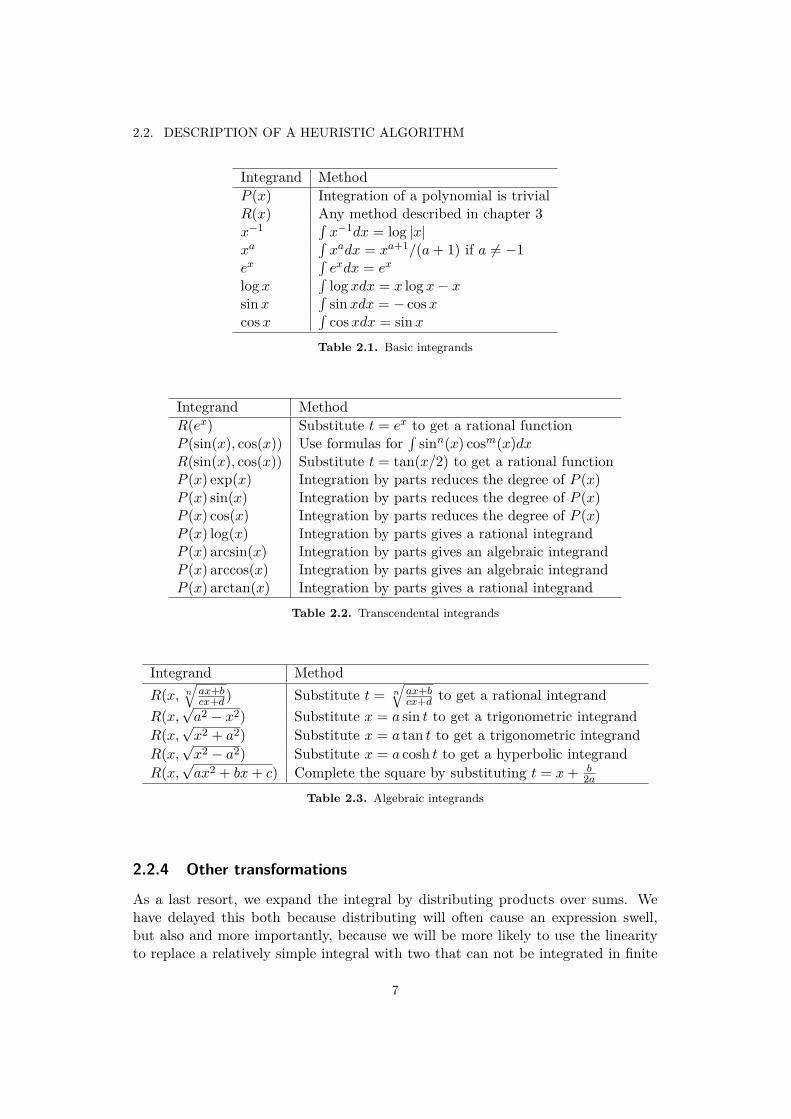
After the use of linearity, the integrand is matched to a list of special forms. Thisincludes all elementary functions along with a number of composite types listed intables 2.1-2.3, where P (x) denotes a polynomial in x and R(x) denotes a rationalfunction in x.

6

2.2. DESCRIPTION OF A HEURISTIC ALGORITHM

Integrand MethodP (x) Integration of a polynomial is trivialR(x) Any method described in chapter 3x−1 ∫

x−1dx = log |x|xa

∫xadx = xa+1/(a+ 1) if a 6= −1

ex∫exdx = ex

log x∫

log xdx = x log x− xsin x

∫sin xdx = − cosx

cosx∫

cosxdx = sin xTable 2.1. Basic integrands

Integrand MethodR(ex) Substitute t = ex to get a rational functionP (sin(x), cos(x)) Use formulas for

∫sinn(x) cosm(x)dx

R(sin(x), cos(x)) Substitute t = tan(x/2) to get a rational functionP (x) exp(x) Integration by parts reduces the degree of P (x)P (x) sin(x) Integration by parts reduces the degree of P (x)P (x) cos(x) Integration by parts reduces the degree of P (x)P (x) log(x) Integration by parts gives a rational integrandP (x) arcsin(x) Integration by parts gives an algebraic integrandP (x) arccos(x) Integration by parts gives an algebraic integrandP (x) arctan(x) Integration by parts gives a rational integrand

Table 2.2. Transcendental integrands

Integrand MethodR(x, n

√ax+bcx+d) Substitute t = n

√ax+bcx+d to get a rational integrand

R(x,√a2 − x2) Substitute x = a sin t to get a trigonometric integrand

R(x,√x2 + a2) Substitute x = a tan t to get a trigonometric integrand

R(x,√x2 − a2) Substitute x = a cosh t to get a hyperbolic integrand

R(x,√ax2 + bx+ c) Complete the square by substituting t = x+ b

2a

Table 2.3. Algebraic integrands

2.2.4 Other transformations

As a last resort, we expand the integral by distributing products over sums. Wehave delayed this both because distributing will often cause an expression swell,but also and more importantly, because we will be more likely to use the linearityto replace a relatively simple integral with two that can not be integrated in finite

7

CHAPTER 2. ELEMENTARY TECHNIQUES

terms as the example in section 2.2.1.We can also apply other transformations and simplifications to the integrand

to reduce the number of functions that appear in the integrand. For example, thefollowing identities can be used to remove products of trigonometric functions.

sin(mx) sin(nx) = cos((m− n)x)− cos((m+ n)x)2

sin(mx) cos(nx) = sin((m− n)x) + sin((m+ n)x)2

cos(mx) cos(nx) = cos((m− n)x) + cos((m+ n)x)2

Similarly, one can convert products of trigonometric and exponential functions tocomplex exponentials with the following.

sin(x) = 1csc(x) = eix − e−ix

2i

cos(x) = 1sec(x) = eix + e−ix

2

tan(x) = 1cot(x) = eix − e−ix

ieix + ie−ix

If hyperbolic functions are not converted to exponentials as part of the automaticsimplification, it may be useful to do so during integration. The formulas for con-verting hyperbolic functions are of course analogous to the ones above.

The tables of integrands and methods in the previous sections was chosen suchthat once a rule is applied, it will eventually lead to an elementary expression forthe integral. Thus, there is no problem with non-terminating rewrite sequences ortrouble caused by choosing the wrong rule when several apply. However, many ofthe substitutions can be helpful even when this cannot be guaranteed, if treatedwith some care. For example, the substitution t = n

√ax+bcx+d transforms

∫f(x, n

√ax+ b

cx+ d)dx =

∫f(dt

n − ba− ctn

, t)dxdtdt

Although it is not certain that the latter is an easier problem, it will often be thecase, so it makes sense to try this transformation even when f is not a rationalfunction.

It is also possible to let the users define their own functions and integrationrules, in which case they could be applied last to avoid any interference with thebuilt-in rules.

8

2.3. USES FOR HEURISTIC ALGORITHMS

2.3 Uses for heuristic algorithmsThere are several reasons for using a heuristic, rule-based method despite the exis-tence of definitive decision procedures like Risch’s algorithm.

1. Heuristic methods are often more efficient for simple problems. To quoteGeddes et al. [12], “the heuristic methods solve a trivial problem in trivialtime, a highly desirable feature”. For this reason, heuristics are actually triedin computer algebra systems such as Maple prior to using an algorithmicapproach.

2. The Risch algorithm will usually use only exponentials and logarithms to ex-press the result, even when it could be expressed in a simpler way for exampleby using inverse trigonometric functions. It is possible to convert the complexexponentials and logarithms to trigonometric functions, or to extend Risch’salgorithm to work directly with these functions but doing so would complicatealready complicated code. Heuristic methods, on the other hand, will usuallyexpress the integral in a similar way to what a human would do.

3. Heuristics are considerably easier to understand and implement, requiringnothing beyond introductory calculus. Risch’s algorithm on the other handrequires a great deal of abstract algebra and algebraic algorithms. As a con-sequence, it is simple to extend the heuristic by adding new rules. ExtendingRisch’s algorithm to include new classes of functions requires significant de-velopments of the underlying mathematics. Such extensions are at the frontof current research.

There is one additional reason for using heuristic rules rather than Risch’s al-gorithm, and that is the ability to generate an understandable derivation of theresult. It is relatively simple to modify a rule-based integration procedure to printthe rules it uses to compute the integral, and to include some additional explana-tions if necessary. By design, the heuristic will try the same rules as a human, sothe proof will look similar to what a human would produce.

In theory it is also possible to modify Risch’s algorithm to generate a proof,but the proof will not be comprehensible to most humans as it relies heavily onLiouville’s theorem.

9

Chapter 3

Integration of rational functions

It turns out that integrating rational functions are of fundamental importance to anyintegration algorithm. Not only are the rational functions a common and interestingclass of functions, but many other types of integrals can also be reduced to integralsof rational functions by applying suitable substitutions. This was the idea behindmany of the rules in the previous chapter.

3.1 The naive methodWe begin by showing that the naive method taught in calculus courses is correct,and at least in theory capable of integrating any rational function p

q .By the fundamental theorem of algebra we know that the denominator q can

be written as a product of linear factors ∏ki=1 q

eii . As appendix A shows, we can

use partial fraction decomposition to express pq as ∑k

i=1∑eij=1

rij

qji, where all rij are

constants. Without loss of generality, we can assume that the factors are monic.This allows us to express the integral as follows∫

rij

qji=

rij log(qi) if j = 1,rij

(1−j)qj−1i

otherwise.

This proves the following simple theorem which can be interpreted as a specialcase of Liouville’s theorem (4.16).

Theorem 3.1 Let f ∈ Q(x). Then∫f is elementary and∫

f = v0 +n∑i=1

ci log vi

where all ci ∈ Q, and all vi ∈ Q(x), Here Q denotes the algebraic closure of therational numbers, i.e. the algebraic numbers.

From a computational point of view, this method is not satisfactory. First,although the factorization exists, we cannot in general represent the factors of a

11

CHAPTER 3. INTEGRATION OF RATIONAL FUNCTIONS

5th or higher degree polynomial using nested radicals. (This is the well-knownAbel-Ruffini theorem). Secondly, even when we can represent the factors, it isstill difficult to actually compute the factorization. In other words, we should tryto avoid factoring as long as possible. The following sections will discuss bettermethods for integrating rational functions.

3.2 Hermite’s method for determining the rational part

If we are to integrate a rational function we can use the division algorithm to splitthe integrand into a polynomial and a proper fraction. The polynomial part istrivial to integrate so we will concentrate on the fraction.

After performing a square-free factorization (cf. appendix B) of the denominatorfollowed by a partial fraction decomposition, the fractions will be of the form qi/r

ii

where qi and ri are polynomials in x, deg(qi) < deg(ri) and ri is square-free.We integrate each such fraction in turn. To increase readability, we omit the

subscript in the remainder of the section, letting r denote one of the square-free riand q denote the corresponding qi. The condition that r is square-free implies thatgcd(r, r′) = 1, so the extended euclidean algorithm computes polynomials a and b,such that

ar + br′ = 1

We can use this to reduce the degree of the denominator, as shown in the followingcomputation

∫q

ri=∫q(ar + br′)

ri=∫

qa

ri−1 +∫qbr′

ri

=∫

qa

ri−1 −qb

(i− 1)ri−1 +∫ (qb)′

(i− 1)ri−1

= − qb

(i− 1)ri−1 +∫ (i− 1)qa+ (qb)′

(i− 1)ri−1

which holds for any i > 1. When i = 1 we use Rothstein-Trager’s method describedin the next section.

3.3 Rothstein - Trager’s method for the logarithmic part

In the previous section we removed any repeated factors from the denominator, sohere we assume that the integrand q/r is a proper fraction where r is square-freeand monic. Let the factorization of r be

r =n∏i=1

(x− ai)

12

3.3. ROTHSTEIN - TRAGER’S METHOD FOR THE LOGARITHMIC PART

where all ai are different. As we saw in section 3.1, this integral is just a sum oflogarithms of the factors of r, i.e.∫

q

r=

n∑i=1

ci log(x− ai)

Notice that in some cases it may not be necessary to factor the denominatorcompletely. For example,

∫2x/(x2 − 2)dx = log(x2 − 2) can be computed and

expressed without introducing the extraneous algebraic extension√

2 by factoringx2−2 = (x+

√2)(x−

√2). The problem of expressing an integral using the minimal

number of algebraic extensions was solved independently by Rothstein and Trager.Let ∫

q

r=

n∑i=1

ci log(vi)

be the expression of the integral using the fewest possible algebraic extensions. Thevi are square-free and we can also assume that they are relatively prime withoutintroducing new algebraic extensions, since

c1 log pq + c2 log qr = c1 log p+ (c1 + c2) log q + c2 log r

Lemma 3.2 Let∫ qr = ∑n

i=1 ci log(vi) where r is a monic polynomial and the viare monic, square-free and relatively prime polynomials. Then

r =n∏j=1

vj and q =n∑i=1

civ′i∏j 6=i

vj

Proof Differentiating and cross-multiplying the denominators gives

qn∏j=1

vj = rn∑i=1

civ′i∏j 6=i

vj

Notice that vi has no factor in common with v′i (since the vi are square-free) and nofactor in common with ∏j 6=i vj (since they are relatively prime). Hence vj dividesevery term in the sum on the right hand side except the one where i = j, so itcannot be a factor of the sum. Instead, vi must be a factor of r for all i, so ∏ vi | r.Conversely, r is a factor of the right hand side but has no factor in common with q,so r | ∏ vi. Since r and all vi are monic, we can conclude that r = ∏

vi as desired.The expression for q then follows immediately. �

At this point, it might be a good idea to recall that for all a, b, n

gcd(a+ nb, b) = gcd(a, b)

13


This theorem is used repeatedly in the following computation.

gcd(q − clr′, vk) = gcd(n∑i=1

civ′i∏j 6=i

vj

− cl n∑i=1

v′i∏j 6=i

vj

, vk)= gcd(ckv′k

∏j 6=k

vj − clv′k∏j 6=k

vj , vk)

= gcd((ck − cl) v′k∏j 6=k

vj , vk)

={

gcd(0, vk) = vk if k = l

1 otherwise

The last equality uses the fact that vk has no factor in common with either v′k or∏j 6=k vj , and ck 6= cl if k 6= l. Once we know the ci, we can use the computations

above to obtain the vi by

gcd(q − cir′, r) = gcd(q − cir′,n∏j=1

vj)

=n∏j=1

gcd(q − cir′, vj)

= vi

Notice that greatest common divisors and derivatives are computed using only ra-tional operations, so they do not introduce any new algebraic extensions.

To obtain the ci, we observe that they are precisely the numbers such thatgcd(q − cir′, r) 6= 1, or equivalently, numbers such that deg(gcd(q − cir′, r)) > 0.According to theorem C.7 in the appendix, resx(q − cir

′, r) = 0 if and only ifdeg(gcd(q− cir′, r)) > 0, so it suffices to compute resx(q− cr′, r) and find the roots.The degree of resx(q−cr′, r) as a polynomial in c can not exceed the degree of r as apolynomial in x, but factoring the resultant may be easier since it can have repeatedfactors. Repeated factors can be found quickly using the square-free factorizationdescribed in appendix B. This proves the following theorem.

Theorem 3.3 Let p, q ∈ Q[x] be relatively prime polynomials such that q is monicand square-free. Let S be the set of distinct zeros to resx(q − cr′, r). Then∫

p

q=∑c∈S

c log(gcd(q − cr′, r))

is the expression for the integral which uses the fewest possible algebraic extensionsof Q.

We will finish the section with an example by Tobey of a rational function whosedenominator is difficult to factor while the integral only requires a single algebraicextension of degree 2.

14

3.3. ROTHSTEIN - TRAGER’S METHOD FOR THE LOGARITHMIC PART

Example 3.4

Compute the integral∫ 7x13 + 10x8 + 4x7 − 7x6 − 4x3 − 4x2 + 3x+ 3

x14 − 2x8 − 2x7 − 2x4 − 4x3 − x2 + 2x+ 1 dx

In this example,

q = 7x13 + 10x8 + 4x7 − 7x6 − 4x3 − 4x2 + 3x+ 3r = x14 − 2x8 − 2x7 − 2x4 − 4x3 − x2 + 2x+ 1

so

resx(q − cr′, r) =− 2377439676624535552c14 + 16642077736371748864c13

− 45765713775022309376c12 + 58247272077301121024c11

− 23922986746034388992c10 − 17682207594894983168c9

+ 15861980342479323136c8 + 3417569535147769856c7

− 3965495085619830784c6 − 1105137974680936448c5

+ 373796667906787328c4 + 227528406551957504c3

+ 44693079858420224c2 + 4063007259856384c+ 145107402137728

=− 145107402137728(4c2 − 4c− 1

)7

The resultant has only two distinct roots c1 = (1 +√

2)/2 and c2 = (1 −√

2)/2.Computing the greatest common divisors gives

gcd(q − c1r′, r) = x7 −

√2x2 − (1 +

√2)x− 1

gcd(q − c2r′, r) = x7 +

√2x2 − (1−

√2)x− 1

and thus the integral∫q

rdx = (1 +

√2)

2 log(x7 −√

2x2 − (1 +√

2)x− 1)

+ (1−√

2)2 log(x7 +

√2x2 − (1−

√2)x− 1)

3.3.1 The Lazard - Rioboo - Trager improvementAlthough the Rothstein-Trager algorithm can save us some factoring and does suc-ceed in expressing the integral using a minimal number of algebraic extensions, theimprovement comes at the cost of several gcd computations over algebraic numberfields. As these gcd computations tend to be expensive (both in terms of run-ning time and programming time), we would like some other way of evaluatinggcd(q(x), p(x) − αq′(x)). Such a method was discovered and published in 1990 byLazard and Rioboo [18] who also remarked that the method had been discovered in-dependently (but not published) by Trager while implementing the Rothstein-Trager

15


algorithm in Axiom. Lazard and Rioboo’s statement and proof is not entirely clearand, according to Mulders [22], the wrong interpretation was used by Geddes et al.[12] and also implemented in Axiom 2.0.

Theorem 3.5 Let q(x) and r(x) be relatively prime polynomials with deg p(x) <deg q(x) and q(x) square-free as above. Let Si(x, y) be the remainder of degree i inthe subresultant PRS of q(x) and p(x) − yq′(x) and α a zero of multiplicity n ofresx(q(x), p(x)− yq′(x)). Then

gcd(q(x), p(x)− αq′(x)) ={q(x) if n = deg(qx)pp(Sn)(x, α) if n < deg(qx)

We will omit the proof because the technical difficulties would take us too far afield.The interested reader may consult for example Bronstein’s book [4].

16

Chapter 4

Liouville’s theorem

This chapter is concerned with proving a theorem of Liouville, which gives a preciseform of the integral, if it is elementary. Before stating and proving the theorem, weneed some concepts from differential algebra.

4.1 Differential algebraDefinition 4.1 Let F be a field. A map ∂ : F→ F such that

∂(f + g) = ∂f + ∂g

∂(fg) = g∂f + f∂g

is called a derivation. The derivative ∂f is also written f ′.

Definition 4.2 A field F equipped with a derivation ∂ is called a differential field.

Definition 4.3 An element c of a differential field is said to be constant if ∂c = 0.

Lemma 4.4 Many of the common rules for derivatives hold in this algebraic set-ting. For example:

∂0 = ∂1 = 0

∂(f/g) = (∂f)g − f∂gg2

Proof

∂0 = ∂(0 + 0) = ∂0 + ∂0 = 2∂0 =⇒ ∂0 = 0∂1 = ∂(1 · 1) = 1 · ∂1 + 1 · ∂1 = 2∂1 =⇒ ∂1 = 0

To prove the quotient rule, notice that

0 = ∂1 = ∂(g · g−1) = g∂(g−1) + g−1∂g

17

CHAPTER 4. LIOUVILLE’S THEOREM

which we can solve for ∂g−1 to get

∂(g−1) = −∂gg2

By applying the product rule

∂(f/g) = ∂(fg−1) = ∂f

g− f∂g

g2 = (∂f)g − f∂gg2

�

Corollary 4.5 The set of all constants in F is a subfield of F. If F has characteristic0, then the constant subfield contains Q.

Proof The field structure follows immediately from the definition and the previouslemma. It is well known that any field of characteristic 0 must contain Q. �

Definition 4.6 A field E is an extension field of F if there exists an injective ho-momorphism φ : F→ E. We also say that F is a subfield of E.

Definition 4.7 Let E and F be differential fields. The field E is a differentialextension field of F if it is an extension field and the homomorphism commuteswith the derivation, i.e. if there exists an injective homomorphism φ : F → E andφ(∂f) = ∂φ(f) for all f ∈ F.

The interpretation of definition 4.6 is that there exists a subset of E isomorphic toF and the interpretation of definition 4.7 is that the derivations coincide on thissubset.

Definition 4.8 Let E be a differential extension field of F. An element θ ∈ E issaid to be algebraic over F if there exist a polynomial p ∈ F[x] such that p(θ) = 0.If there is no such polynomial, then θ is transcendental over F.

Definition 4.9 Let E be a differential extension field of F. An element θ ∈ E issaid to be logarithmic over F if there exist a u ∈ F such that θ′ = u′

u . If this is thecase, we write θ = log(u).

Definition 4.10 Let E be a differential extension field of F. An element θ ∈ E issaid to be exponential over F if there exist a u ∈ F such that θ′ = u′θ. If this is thecase, we write θ = exp(u).

The alert reader may have noticed that the definitions of logarithms and expo-nentials are given in the form of differential equations. As usual, the solution maynot be unique, so in the remainder of this text exp(u) and log(u) should be inter-preted as unspecified exponential and logarithmic elements with inner derivativeu′. In the ordinary case of real, differentiable functions we can of course avoid theproblem by specifying initial values, viz. exp(0) = 1 and log(1) = 0.

18

4.1. DIFFERENTIAL ALGEBRA

Theorem 4.11 Using only the previous definitions of exponentials and logarithmsin a differential field, we can deduce the following useful properties.

1. log(u) is unique up to an additive constant.

2. exp(u) is unique up to a multiplicative constant.

3. log(exp(u)) = u+ c where c is a constant.

4. log(exp(u)) = cu where c is a constant.

5. log(u) + log(v) = log(uv)

6. exp(u) exp(v) = exp(u+ v)

Proof

1. Let logα(u) and logβ(u) both satisfy definition 4.9. Then

(logα(u)− logβ(u)

)′= u′

u− u′

u= 0

Hence logα(u)− logβ(u) is constant.

2. Let expα(u) and expβ(u) both satisfy definition 4.10. Then(expα(u)expβ(u)

)′=u′ expα(u) expβ(u)− u′ expα(u) expβ(u)

expβ(u)2 = 0

Hence expα(u)expβ(u) is constant.

3. To prove that log(exp(u)) = u+ c, it suffices to take the derivative of the lefthand side, i.e.

(log(exp(u)))′ = (exp(u))′exp(u) = u′ exp(u)

exp(u) = u′

Hence log(exp(u)) = u+ c for some constant c.

4. Similarly, one can prove that exp(log(u)) = cu by differentiating the quotient(exp(log(u))u

)′= u′ exp(log(u))− u′ exp(log(u))

u2 = 0

Hence exp(log(u)) = cu for some constant c.

5. Proving log(u) + log(v) = log(uv) is easy.

(log(u) + log(v))′ = u′

u+ v′

v= u′v + v′u

uv= (log(uv))′

19


6. Proving exp(u) exp(v) = exp(u+v) may be less obvious but not very difficult.

(exp(u) exp(v))′ = u′ exp(u) exp(v) + v′ exp(u) exp(v) == (u+ v)′ exp(u) exp(v)

Recall that if θ′ = f ′θ, then θ = exp(f) by definition. Thus exp(u) exp(v) =exp(u+ v).

�

Following Geddes et al. [12], we will now investigate how some polynomialsinvolving logarithms, exponentials or algebraic functions behave under differentia-tion.

Theorem 4.12 Let F(θ) be a differential extension field of F with the same field ofconstants, where θ is logarithmic over F. Let p(θ) ∈ F[θ] be a polynomial of degreen > 0. Then p(θ)′ ∈ F[θ] and

deg p(θ)′ ={n− 1 if cn is constant,n otherwise.

Proof

p(θ)′ =(

n∑i=0

ciθi

)′=

n∑i=0

(c′iθ

i + iciθi−1θ′

)=

n−1∑i=0

(c′i + (i+ 1)ci+1θ

′) θi + c′nθn

It is obvious that deg p(θ)′ = n if and only if cn is non-constant. We must showthat c′n−1 + ncnθ

′ 6= 0 if cn is constant. Therefore suppose that cn is constant andc′n−1 +ncnθ

′ = 0. Then (ncnθ+ cn−1)′ = nc′nθ+ncnθ′+ c′n−1 = 0 contradicting the

assumption that the extension had no new constants. �

Theorem 4.13 Let F(θ) be a differential extension field of F with the same field ofconstants, where θ is exponential over F. Let p(θ) ∈ F[θ] be a polynomial of degreen > 0. Then p(θ)′ ∈ F[θ] and deg p(θ) = n

Proof

p(θ)′ =(

n∑i=0

ciθi

)′=

n∑i=0

(c′iθ

i + iciθi−1θ′

)=

n∑i=0

(c′i + iciu

′) θishows that p(θ)′ ∈ F[θ]. We must show that c′n + ncnu

′ 6= 0. But if c′n + ncnu′ = 0,

then (cnθn)′ = (c′n + ncnu′) θn = 0, so cnθ

n is a constant. This contradicts theassumption that the extension had no new constants. �

20

4.2. LIOUVILLE’S THEOREM

Definition 4.14 A field E is an elementary extension of F if it is a differentialfield extension of F and there exists a finite tower of fields

F = E0 ⊂ E1 ⊂ . . . ⊂ Ek−1 ⊂ Ek = E

such that each Ei = Ei−1(θi) where θi is algebraic, logarithmic or exponential overEi−1.

Definition 4.15 Let E be a differential extension field of F. An element θ ∈ E issaid to be elementary over F if F (θ) is an elementary extension field over F.

4.2 Liouville’s theoremWe saw in the chapter on integration of rational functions that if f ∈ Q(x), then∫f = v0 + ∑n

i=1 ci log vi where ci are constants in Q and vi ∈ Q(x). (As usual,F is the algebraic closure of F.) We shall now see how this generalizes to largerdifferential fields.

Theorem 4.16 (Liouville)Let F be a differential field, and let f ∈ F. If

∫f is in an elementary extension E

of F with the same field of constants K, then∫f = v0 +

n∑i=1

ci log vi

where all ci ∈ K, and all vi ∈ F

Proof Let E = F(θ1, θ2, . . . , θk) be a field containing the integral. We will use induc-tion on the number of extensions to prove the theorem. The case of no extensions isobvious, since then

∫f = v0 where v0 ∈ F. We now want to prove that the theorem

is true for i+ 1 extensions, given that it is true for i extensions.Obviously, f ∈ F(θ1), so by the induction assumption∫

f = v0(θ1) +n∑i=0

ci log vi(θ1)

where the v0, v1, . . . , vn are rational functions in θ1. What remains is proving thatthe vi are free of θ1. To improve readability, we will omit the subscript and denoteθ1 just by θ. We now have three cases depending on whether θ is algebraic, atranscendental logarithm or a transcendental exponential.

4.2.1 Transcendental extensionsIf θ is transcendental over the field F, then F[θ] is an euclidean domain and thereforealso a unique factorization domain. This allows us to treat elements of F[θ] and F(θ)

21


as polynomials or rational functions in θ, and to use well known algorithms such asthe euclidean algorithm and partial fraction decomposition.

By using the logarithm rules

log(fg) = log f + log glog(f/g) = log f − log g

we can assume that v1, . . . , vn are irreducible polynomials in F[θ]. Unless vi isindependent of θ, we can also factor out the leading coefficient, to make the polyno-mial monic. Furthermore, if two of the logarithms are equal, we can rewrite themas a single term by combining the coefficients. Hence we may safely assume thatv1, . . . , vn are all distinct.

The element v0 is a rational expression in F(θ). We can use the euclideanalgorithm to separate v0 into a polynomial part and a proper fraction. After apartial fraction expansion,

v0 = r0(θ) +k∑i=1

ei∑j=1

rij(θ)qi(θ)j

where r0, rij , qi ∈ F[θ], deg(rij) < deg(qi) and qi irreducible. Here we can alsoassume that the denominators are monic.

Since∫f = v0(θ) +∑n

i=1 ci log vi(θ), it follows that

f = r0(θ)′ +k∑i=1

ei∑j=1

(rij(θ)′qi(θ)j

− jrij(θ)qi(θ)′qi(θ)j+1

)+

n∑i=0

civi(θ)′vi(θ)

The important point of this equation is that the left hand side is free of θ. Aftermultiplying both sides of this equation by

d(θ) = lcm(q1(θ)e1+1, . . . , qk(θ)ek+1, v1(θ), . . . , vn(θ))

we obtain a polynomial equation in F[θ]

d(θ)f = r0(θ)′d(θ) +k∑i=1

ei∑j=1

(rij(θ)′d(θ)qi(θ)j

− jrij(θ)qi(θ)′d(θ)qi(θ)j+1

)

+n∑i=0

civi(θ)′d(θ)vi(θ)

(4.1)

Logarithmic extensions

If θ is a transcendental logarithm, then by recalling that qi(θ) is monic and usingtheorem 4.12 we see that deg(qi(θ)′) < deg(qi(θ)). Since qi(θ) is irreducible, thismeans that qi(θ)′ and qi(θ) have no common factor.

For any qi, it is easy to see that all terms in 4.1 except ekriek (θ)qi(θ)′d(θ)qi(θ)ek+1 are

divisible by qi(θ), and hence qi(θ) must divide ekriek (θ)qi(θ)′d(θ)qi(θ)ek+1 too. But we have

22


established that qi(θ) is relatively prime to rij(θ) and qi(θ)′, so qi(θ) divides d(θ)qi(θ)ek+1 .

This is only possible if qi(θ) ∈ F.Let us consider the term r0(θ) next. If deg(r0(θ)′) > 0 then the right hand side

of equation 4.1 would have a higher degree than the left hand side. This is clearlya contradiction, so deg(r0(θ)′) = 0 and by theorem 4.12 either deg(r0(θ)) = 0 ordeg(r0(θ)) = 1 with the coefficient of θ being a constant. In the latter case, wecan move the θ-term into the sum ∑n

i=0 ci log vi since θ is itself a logarithm and thecoefficient is constant. Without loss of generality, we assume that r0 is free of θ.

If we insert what we have determined so far into equation 4.1, we arrive at

fn∏i=1

vi(θ) = v′0

n∏i=1

vi(θ) +n∑i=1

civi(θ)′

∏ni=1 vi(θ)

vi(θ)

where vi(θ) divides all terms except vi(θ)′∏n

i=1 vi(θ)vi(θ) . To divide this term, vi(θ) must

divide vi(θ)′, which is only possible (recall theorem 4.12) if vi is free of θ.This proves that v0, v1, . . . , vn ∈ F, as desired.

Exponential extensions

Let θ be a transcendental exponential. As before, we obtain the polynomial equation4.1.

Just like the logarithmic case, if deg(r0(θ)′) > 0 then the right hand side ofthis equation would have a higher degree than the left hand side. We deduce thatdeg(r0(θ)′) = 0 and by theorem 4.13 deg(r0(θ)) = 0.

Unlike the logarithmic case, it is not easy to see whether qi(θ) is a factor ofqi(θ)′. For this we need an additional lemma:

Lemma 4.17 For any p(θ) ∈ F[θ], p(θ) | p(θ)′ if and only if p is of the form fθn

with f ∈ F.

Proof (⇐) It is clear that if p is of the form above, fθn | (f ′ + nfu′) θn = (fθn)′.(⇒) On the other hand, if p(θ) | p(θ)′, then p(θ) = d(θ)(p(θ)′). Comparing thedegrees (using theorem 4.13), we see that deg d(θ) = 0. If p is not a monomial, ithas at least two non-zero terms anθn and amθm. These terms satisfy

anθnd = (a′n + nanu

′)θn

amθmd = (a′m +mamu

′)θm

Eliminating d givesa′mam− a′nan

= (n−m)u′

This can be used to show that(anam

θn−m)′

=(a′nam− a′man

a2m

)θn−m + (n−m)u′ an

amθn−m

=(a′mam− a′nan− (n−m)u′

)anam

θn−m = 0

23


contradicting the assumption that θ is a transcendental non-constant. �

Continuing with the exponential case of Liouville’s theorem, we see that qi(θ)divides all terms in 4.1 except ekriek (θ)qi(θ)′d(θ)

qi(θ)ek+1 . Since ri(θ) is relatively prime toqi(θ), and d(θ) contain no power of qi(θ) greater than qi(θ)ek+1, qi(θ) must divideqi(θ)′ to divide this term. By the lemma above, qi(θ) must be a monomial todivide qi(θ)′. The assumption that qi(θ) is monic and irreducible then implies thatqi(θ) = θ unless qi(θ) ∈ F.

Observe that when θ is exponential, we can assume that vi 6= θ because log θ =log(expu) = u + c ∈ F. If we insert what we have determined so far into equation4.1, we obtain

fd(θ) = r′0d(θ) +e∑j=1

(r′jd(θ)θj

− jrjθ′d(θ)

θj+1

)+

n∑i=0


= r′0d(θ) +e∑j=1

(r′j − jrju′)d(θ)θj

+n∑i=0


whered(θ) = lcm(θe, v1(θ), . . . , vn(θ)) = θe

n∏i=1

vi

Notice that θ divides the left hand side and all terms on the right hand side except(r′e−ereu′)d(θ)

θe . This is a contradiction, so no θ can appear in the rational part. Simi-larly, all terms except ci vi(θ)′d(θ)

vi(θ) are divisible by vi(θ). Again, this is a contradiction,so all vi are free of θ.

This proves that v0, v1, . . . , vn ∈ F, as desired.

4.2.2 Algebraic extensionsFinally, suppose that θ is algebraic over F, so there exists a polynomial p ∈ F[x]such that p(θ) = 0. Now, with θ algebraic, F[θ] is no longer isomorphic to theordinary polynomial ring F[t] in the new variable t. It should come as no surprisethat the proof of the algebraic case of Liouville’s theorem is fundamentally differentfrom the transcendental cases above.

Definition 4.18 Let θ be algebraic over a field F. The monic polynomial of leastdegree such that p(θ) = 0 is called the minimal polynomial of θ over F.

It is not difficult to see that the minimal polynomial is unique. If there weretwo monic polynomials of least degree such that p(θ) = q(θ) = 0, then p(t) − q(t)would be a a polynomial of lower degree but still satisfy p(θ)− q(θ) = 0.

Lemma 4.19 Let θ be algebraic over a field F, and let p(t) be the minimal polyno-mial of θ. Then F(θ) is isomorphic to F[t]/ 〈p(t)〉, where 〈p(t)〉 is the ideal generatedby p(t).

24


Proof Define a map φ : F[t]/ 〈p(t)〉 → F(θ), by φ([q(t)]) = q(θ) where [q(t)] isthe equivalence class of q(t) mod p(t). It is obviously a field homomorphism. It issurjective because imφ is a field containing both F and θ, and F(θ) is defined as thesmallest such field. It is injective because q(θ) = r(θ) =⇒ q(θ) − r(θ) = 0 so θ isa zero of q(t)− r(t). Then p(t) | q(t)− r(t) since p(t) is the minimal polynomial ofθ, so [q(t)] = [r(t)]. �

Definition 4.20 Let p be the minimal polynomial of θ. The roots of p (in thealgebraic closure F) are called the conjugates of θ.

Definition 4.21 Let F(θ) be an algebraic extension of F and let the conjugates ofθ be {θ0, θ1, . . . , θk}. We define the norm N : F(θ)→ F and trace Tr : F(θ)→ F ofan element v(θ) in F(θ) by

N(v(θ)) =k∏i=0

v(θi)

Tr(v(θ)) =k∑i=0

v(θi)

We are now ready to continue with the proof of Liouville’s theorem. By theinduction hypothesis ∫

f = v0(θ) +n∑i=0

ci log vi(θ)

sof = v0(θ)′ +

n∑i=0

civi(θ)′vi(θ)

where it remains to prove that the vi are free of θ.Let {θ0, θ1, . . . , θk} be the set of conjugates of θ. Since all F(θj) are isomorphic

to F[t]/ 〈p(t)〉, it follows that

f = v0(θj)′ +n∑i=0

civi(θj)′vi(θj)

for all j. Summing the equations over all conjugates gives

(k + 1)f =k∑j=0

(v0(θj)′ +

n∑i=0

civi(θj)′vi(θj)

)=

=k∑j=0

v0(θj)′ +n∑i=0

civi(θj)′

∏j 6=i vi(θj)∏k

j=0 vi(θj)=

= Tr(v0(θ))′ +n∑i=0

ciN(vi(θ))′N(vi(θ))

25


so ∫f = Tr(v0(θ))

k + 1 +n∑i=0

cik + 1 logN(vi(θ))

is another expression for the integral which does not use any algebraic extensionsof F. This concludes the proof of Liouville’s theorem.

4.2.3 Strong form of Liouville’s theoremThe proof of Liouville’s theorem in the previous section depended on the assumptionthat the constant subfield of E containing the integral was equal to the constantsubfield of F. It is however possible to remove this restriction on the constants toobtain the following theorem.

Theorem 4.22 Let F be a differential field containing the integrand f and let K bethe subfield of constants in F. If

∫f is in an elementary extension E of F, then∫

f = v0 +n∑i=1

ci log vi

for some v0 ∈ F, ci ∈ K, and vi ∈ F(c1, c2, . . . , cn).

For a proof, see for example [4].

4.3 ExamplesWe will now give an example of how Liouville’s theorem can be used to prove thata function defined as an integral is non-elementary.

Example 4.23 The function∫ex

2dx is not elementary.

Proof The integrand θ = ex2 is in the field Q(x, θ). Suppose there is an elementary

expression for∫θ. Then according to Liouville’s theorem∫

θ = p

q+

n∑i=1

ci log(vi)

where p, q and all vi are polynomials in Q(x)[θ]. Differentiating and cross-multiplyingthe denominators gives

q2θ∏j

vj = (p′q − pq′)∏j

vj + q2n∑i=1

civ′i

∏j 6=i

vj

where we can assume without loss of generality that all vi are distinct and relativelyprime. Since log θ = x2 ∈ Q(x), we can also assume that no vi is divisible by θ.Observe that for any k, all terms above except ckv′k

∏j 6=k vj are divisible by vk. To

26

4.3. EXAMPLES

divide this last term we would require that vk divides v′k which according to lemma4.17 is only possible if vk = fθm. By the assumption, this is not the case, so all viare free of θ.

Next, observe that q2 must divide (p′q−pq′)∏j vj which implies that q2 divides(p′q− pq′). As before, q | q′ implies that q = fθm for some f ∈ Q(x), k ∈ N. Hence,the quotient p/q can be written as a linear combination of (positive and negative)powers of θ, viz.

p = p

q=

deg p∑i=0

pifθi−deg q =

deg p−deg q∑i=− deg q

piθi

p′ =

deg p−deg q∑i=− deg q

piθi

′ = deg p−deg q∑i=− deg q

(p′i + 2ixpi)θi

Replacing p/q by p in the expression for the integral gives

θ = p′ +n∑i=1

civ′ivi

from which one can immediately see that p′ and thus p must be a polynomial inQ(x)[θ] of degree one. To satisfy the equation

θ = p′0 + (p′1 + 2xp1)θ +n∑i=1

civ′ivi

p1 must be a solution to the differential equation p′1 + 2xp1 = 1 in Q(x) and theother terms must cancel.

Let s(x)/t(x) be a solution to y′ + 2xy = 1 with s, t ∈ Q[x]. After cross-multiplying the denominators to get s(x)′t(x)− s(x)t(x)′ + 2xs(x)t(x) = t(x)2, wesee that t(x) must divide t(x)′. This is impossible unless t is a constant, in whichcase we should be looking for solutions in Q[x] to y′ + 2xy = 1. It is, however,clear that the equation can not have polynomial solutions since deg(y′ + 2xy) =1 + deg(y) > deg(1). �

27

Chapter 5

Risch’s algorithm

This chapter will describe the proof of the following theorem:

Theorem 5.1 (Risch, 1969)Let f be a function in F = K(x, θ1, . . . , θn) where K is the field of constants in F andeach θi is a transcendental logarithm or exponential over K(x, θ1, . . . , θi−1). Thenthere exists an algorithm which either computes

∫f as an elementary function over

F if it exists, or proves that∫f is not elementary over F

The proof is by induction on n, the number of transcendental extensions. Thebase case of the induction, n = 0, is integration of rational functions discussedin chapter 3. Assuming that the theorem holds for the field K(x, θ1, . . . , θi−1), wemust prove that it holds for K(x, θ1, . . . , θi) too. For brevity, we will drop thesubscript and denote θi by just θ. We now have two cases depending on whether θis logarithmic or exponential.

Although the proofs are more complicated, the integration methods will ulti-mately turn out to be similar to the ones described in chapter 3, with the exceptionthat integration of a polynomial in θ is non-trivial.

5.1 Logarithmic extensionsLet θ be a logarithm and f ∈ F(θ) We can express f as a p+ q

r where p, q, r ∈ F[θ],and deg(q) < deg(r).

We begin with a decomposition lemma from Davenport et al. [10].

Lemma 5.2 If∫f is elementary, then

∫p and

∫ qr are elementary too, so we can

integrate the polynomial part p, and rational part qr separately.

Proof By Liouville’s principle, if∫f is elementary then

∫f = v0 +

n∑i=1

ci log vi

29

CHAPTER 5. RISCH’S ALGORITHM

sof = p+ q

r= v′0 +

n∑i=1

civ′ivi

=(p+ q

r

)′+

n∑i=1

civ′ivi

Some of the vi are polynomials dependent on θ and some are independent of θ.We’ll assume that the ones independent of θ are v1, v2, . . . , vk. Using lemma 4.12,we see that the derivative of the polynomial p is a polynomial, and the derivativeof the proper fraction q/r is a proper fraction. Recall that the decomposition intoa polynomial part and a proper fraction is unique and apply this to the equationabove.

p = p′ +k∑i=1

civ′ivi

q

r=(q

r

)′+

n∑i=k+1

civ′ivi

Integrating these equations gives∫p = p+

k∑i=1

ci log vi∫q

r= q

r+

n∑i=k+1

ci log vi

so both integrals are elementary as well. �

5.1.1 Polynomial partLet p = ∑

aiθi and p = ∑

biθi. The decomposition lemma above implies that

deg(p)∑i=0

aiθi =

deg(p)∑i=0

(b′i + (i+ 1)bi+1θ

′) θi +n∑

i=k+1civ′ivi

Comparing the degrees, we see that deg(p) = deg(p) unless deg(p) = deg(p) + 1and the leading coefficient in deg(p) is a constant. Equating the coefficients givesai = b′i + (i+ 1)bi+1θ

′ for all i > 0, so

bi =∫ (

ai − (i+ 1)bi+1θ′)+ di

where di is a constant. The value of the constant di+1 is determined by the conditionthat

bi =∫ (

ai − (i+ 1)bi+1θ′)+ di =

=∫ (

ai − (i+ 1)(bi+1 − di+1 + di+1)θ′)

+ di =

=∫ (

ai − (i+ 1)(bi+1 − di+1)θ′)− (i+ 1)di+1θ + di

30

5.1. LOGARITHMIC EXTENSIONS

should be free of θ. Notice that bi+1−di+1 is precisely the integral appearing in theequation for bi+1. We can thus compute the bi starting with the leading coefficientand working our way down to b1. When we equate the coefficients of terms of degreezero, we get

a0 = b′0 + b1θ′ +

n∑i=k

civ′ivi

sob0 +

n∑i=k

ci log vi =∫ (

a0 − b1θ′)+ d0

where the last constant d0, which is not determined by any condition, is the constantof integration.

If some integral in the computation of the bi involves extensions of F other thanθ, then the integral of the polynomial part cannot be elementary.

5.1.2 Rational partThe previous section treated the polynomial part of the integrand, so in this sectionwe assume that the integrand is a proper fraction q/r where q and r are polynomialsin θ. After performing a square-free factorization of the denominator, followed by apartial fraction decomposition, the fractions will be of the form qi/r

ii where qi and

ri are polynomials, deg(qi) < deg(ri) and the ri are square-free. We integrate eachsuch fraction in turn.

Lemma 5.3 Let r ∈ F[θ] be a monic square-free polynomial. Then gcd(r, ddxr) = 1.

Proof Let r have the factorization

r =n∏i=0

(θ − ai)

in F[θ] where all ai are distinct. Then the derivative of r with respect to x is

r′ =n∑i=0

(θ′ − a′i)∏i 6=j

(θ − aj)

All terms on the right hand side except one are divisible by θ − aj , but as thelast term is not divisible by θ − aj , the left hand side of the equation cannot beeither. Thus the only possible factors of r does not divide r′, and we can deducethat gcd(r, r′) = 1. �

Corollary 5.4 Let r ∈ F[θ] be a monic square-free polynomial, i.e. under the sameconditions as the lemma above, then there exist polynomials a, b ∈ F[θ] such thatar + br′ = 1.

31


Proof F[θ] is an euclidean domain, so the extended euclidean algorithm gives aand b as desired. �

Returning to the problem of finding the rational part, we get∫q

rk=∫q(ar + br′)

rk=∫

qa

rk−1 +∫qbr′

rk

=∫

qa

rk−1 −qb

(k − 1)rk−1 +∫ (qb)′

(k − 1)rk−1

= − qb

(k − 1)rk−1 +∫ (k − 1)qa+ (qb)′

(k − 1)rk−1

This reduces the degree of the denominator, so we can repeat this step until k = 1.As we shall see, we have fully determined the rational part of the integral when thedenominator no longer has any repeated factors.

5.1.3 Logarithmic partIn the previous section we removed any repeated factors from the denominator, sohere we assume that the integrand is q/r where r is square-free and monic.

Lemma 5.5 Let qr be a proper fraction in F(θ) such that the denominator is square-free. Without loss of generality we can assume that r is monic, so it has the fac-torization r = ∏n

i=1(θ − ai) (in F[θ]) where all ai are different. Then if∫ qr is

elementary, ∫q

r=

n∑i=1

ci log(θ − ai)

Proof From Liouville’s theorem we know that∫q

r= q

r+

n∑i=1

ci log(vi)

or equivalentlyq

r= q′r − r′q

r2 +n∑i=1

civ′ivi

As we did in the proof of Liouville’s theorem, we can assume that the vi are distinct,irreducible, monic polynomials, so after cross-multiplication we get the polynomialequation

qr2∏j

vj = (q′r − r′q)r∏j

vj +n∑i=1

cirr2v′i∏j 6=i

vj

As we can see, r2 divides all terms except (q′r − r′q)r∏j vj . The polynomial rdoes not divide q′r − r′q since it does not divide r′ and is relatively prime to q.Furthermore, it can only divide ∏j vj once, as all vi are irreducible and distinct.

32

5.2. EXPONENTIAL EXTENSIONS

Since r is square-free by assumption, r can divide r at most once, so it must bethe case that r | ∏j vj and r | r. But this means that r3 divides all terms except(q′r − r′q)r∏j vj and since r can divide ∏j vj only once, r2 must divide r. This isa contradiction, so there cannot be any proper rational part. Thus∫

q

r=

n∑i=1

ci log(vi)

q

r=

n∑i=1

civ′ivi

and

q∏j

vj = rn∑i=1

civ′i∏j 6=i

vj

Since every factor of r divides the right hand side, it must divide some vi on theleft hand side too. The vi are irreducible, so every factor of r must in fact be equalto some vi. Conversely, every vi divides all terms in the sum except civ′i

∏j 6=i vj , so

it must divide r instead. We can conclude that the vi are precisely the factors of r.�

If we cancel r = ∏j vj from the last equation in the proof, we obtain

q =n∑i=1

ci(θ′ − a′i)∏j 6=i

(θ − aj)

which we can use to identify the ci with appropriate coefficients in q. When deter-mining the ci, we should remember that they must be constants if the integral iselementary.

The problem with this approach is that it requires a complete factorization ofr. Just like the case with rational functions in chapter 3, we can use the Rothstein-Trager method or the Lazard-Rioboo-Trager method to compute the integral usingthe minimal number of algebraic extensions.

Example 5.6 The logarithmic integral∫ 1

log xdx is not elementary.

Proof Let θ denote log x and notice that the integrand 1θ is a proper fraction with

square-free denominator. It follows from the previous lemma that if the integral iselementary, it must be of the form c log θ. However, (c log θ)′ = c 1

xθ 6=1θ for every

constant c, so the integral can not be elementary. �

5.2 Exponential extensionsIf θ is exponential rather than logarithmic, the only major difference is that thepolynomial part is more complicated to integrate. For reasons that will become

33


clear in the proofs, we express the integrand f ∈ F(θ) as p+ qr where p ∈ F[θ, θ−1],

q, r ∈ F[θ], deg(q) < deg(r) and θ does not divide r. The effect of this representationis that we will handle negative powers of θ in the polynomial part. We will again usea decomposition lemma, similar to the one from Davenport et al. [10], to integratethe p and q

r separately.

Lemma 5.7 If∫f is elementary, then

∫p and

∫ qr are elementary too, so we can

integrate the polynomial part p and rational part qr separately.

Proof By Liouville’s principle, if∫f is elementary then

∫f = v0 +

n∑i=1

ci log vi

so

f = p+ q

r= v′0 +

n∑i=1

civ′ivi

=(p+ q

r

)′+

n∑i=1

civ′ivi

where p+ qr is an expression for v0 such that p ∈ F[θ, θ−1], q, r ∈ F[θ], deg(q) < deg(r)

and θ does not divide r.Some of the vi in the logarithms are polynomials that depend on θ and some

are independent of θ. Assume without loss of generality that v1, v2, . . . , vk areindependent of θ, and that vk+1, vk+2, . . . , vn are monic and not divisible by θ.Unlike the logarithmic case, deg(v′i) = deg(vi), so v′i

viis not a proper fraction. To

remedy the situation, notice that

v′ivi− niu′ =

v′i − niu′vivi

is a proper fraction if ni is the degree of vi and u′ is the inner derivative of θ. Thus

p+ q

r=(p+ q

r

)′+

k∑i=1

civ′ivi

+n∑

i=k+1civ′i − niu′vi

vi+

n∑i=k+1

ciniu′

Using lemma 4.13, one can see that the derivative of p is a polynomial in F[θ, θ−1],and the derivative of q/r is a proper fraction such that θ does not divide the de-nominator. Identifying polynomial parts (in F[θ, θ−1]) and proper fractions withdenominators not divisible by θ gives

p = p′ +k∑i=1

civ′ivi

+n∑

i=k+1ciniu

′

q

r=(q

r

)′+

n∑i=k+1

civ′i − niu′vi

vi

34


Integrating these equations gives

∫p = p+

k∑i=1

ci log vi +n∑

i=k+1ciniu

∫q

r= q

r+

n∑i=k+1

ci(log vi − niu)

so both these integrals are elementary as well. �

5.2.1 Polynomial partLet p = ∑

aiθi and p = ∑

biθi where the index i may take on both positive and

negative values. Equating terms of the same degree in the decomposition lemmaabove gives

a0 = b′0 +k∑i=1

civ′ivi

+n∑

i=k+1ciniu

′

aiθi =

(biθ

i)′

= (b′i + ibiu′)θi if i 6= 0

It is easy to integrate the first equation to get

b0 =∫a0 −

k∑i=1

ci log vi −n∑

i=k+1ciniu

where the vi and ci (for 1 ≤ i ≤ k) are to be chosen in such a way as to cancel anylogarithmic extension in

∫a0.

To compute the coefficients bi, we have to solve differential equations of the form

b′i + iu′bi = ai

known as Risch’s differential equation. The problem of solving Risch’s differentialequation will be discussed further in chapter 6.

5.2.2 Rational partWe now turn to the problem of integrating a proper fraction q/r where q and r arepolynomials in θ with deg(q) < deg(r). Like before, the idea is to use Hermite’sreduction to simplify the integrand, but to do so we need the denominator to satisfygcd(r, r′) = 1. When the denominator was a polynomial in either x or a logarithmθ, it was sufficient to make the denominator square-free. Unfortunately, it is not assimple when θ is an exponential. For example, this fails for the simple polynomialθ, as gcd(θ, θ′) = gcd(θ, u′θ) = θ. The way to avoid this problem is to not only doa square-free factorization, but also factor out the largest power of θ appearing in

35


the denominator. After this factorization and a partial fraction decomposition, thefractions will be of the form qi/r

ii where qi and ri are polynomials, deg(qi) < deg(ri)

and ri is monic, square-free and either equal to θ, or not divisible by θ.

Lemma 5.8 Let r ∈ F[θ] be a monic, square-free polynomial of positive degree,such that θ - r. Then

gcd(r, r′) = 1

Proof Let the factorization of r in F[θ] be

r =n∏i=0

(θ − ai)

where all ai are distinct and non-zero. Then the derivative of r with respect to x is

r′ =n∑i=0

(θ′ − a′i)∏i 6=j

(θ − aj)

All terms on the right hand side, except the one where i = j, are divisible by θ−aj .The only way this last term term can be divisible by θ − aj is if θ − aj | θ′ − a′jAccording to lemma 4.17, this can only happen if aj is zero which contradicts theassumption. Since none of the factors of r divide r′, we can deduce that gcd(r, r′) =1. �

Corollary 5.9 Let r ∈ F[θ] be a monic square-free polynomial not divisible by θ,i.e. under the same conditions as the lemma above, then there exist polynomialsa, b ∈ F[θ] such that ar + br′ = 1.

Proof F[θ] is an euclidean domain, so the extended euclidean algorithm gives aand b as desired. �

Returning to the problem of finding the rational part, we get∫q

rk=∫q(ar + br′)

rk=∫

qa

rk−1 +∫qbr′

rk

=∫

qa

rk−1 −qb

(k − 1)rk−1 +∫ (qb)′

(k − 1)rk−1

= − qb

(k − 1)rk−1 +∫ (k − 1)qa+ (qb)′

(k − 1)rk−1

This reduces the degree of the denominator, so we can repeat this step until k = 1.As we shall see, we have fully determined the rational part of the integral when thedenominator no longer has any repeated factors.

36


5.2.3 Logarithmic partIn the previous section we removed any repeated factors from the denominator, sohere we assume that the integrand is q/r where r is square-free and monic.

Lemma 5.10 Let qr be a proper fraction in F(θ) such that the denominator is

square-free, and not divisible by θ. Without loss of generality we can assume thatr is monic, so it has the factorization r = ∏n

i=1(θ − ai) (in F[θ]) where all ai aredifferent. Then if

∫ qr is elementary,

∫q

r=

n∑i=1

ci log(θ − ai)

Proof From Liouville’s theorem we know that∫q

r= q

r+

n∑i=1

ci log(vi)

or equivalentlyq

r= q′r − r′q

r2 +n∑i=1

civ′ivi

As we did in the proof of Liouville’s theorem, we can assume that the vi are distinct,irreducible, monic polynomials, so after cross-multiplication we get the polynomialequation

qr2∏j

vj = (q′r − r′q)r∏j

vj +n∑i=1

cirr2v′i∏j 6=i

vj

As we can see, r2 divides all terms except (q′r− r′q)r∏j vj . The polynomial r doesnot divide q′r − r′q since it does not divide either of r′ and q (recall lemma 4.17).Furthermore, it can only divide ∏j vj once, as all vi are irreducible and distinct.Since r is square-free by assumption, r can divide r at most once, so it must bethe case that r | ∏j vj and r | r. But this means that r3 divides all terms except(q′r − r′q)r∏j vj and since r can divide ∏j vj only once, r2 must divide r. Thiscontradicts the assumption that r is square-free, so there cannot be any properrational part. Thus ∫

q

r=

n∑i=1

ci log(vi)

q

r=

n∑i=1

civ′ivi

and

q∏j

vj = rn∑i=1

civ′i∏j 6=i

vj

37


Since every factor of r divides the right hand side, it must divide some vi on theleft hand side too. The vi are irreducible, so every factor of r must in fact be equalto some vi. Conversely, every vi divides all terms in the sum except civ′i

∏j 6=i vj , so

it must divide r instead. We can conclude that the vi are precisely the factors of r.�

Just as for the logarithmic extensions, we can obtain the coefficients ci by solvingthe linear system

q =n∑i=1

ci(θ′ − a′i)∏j 6=i

(θ − aj)

but using this approach requires the full factorization of r. As before, we can usethe Rothstein-Trager method or the Lazard-Rioboo-Trager method to avoid thisproblem.

38

Chapter 6

The Risch differential equation

The previous chapter reduced the problem of integrating a polynomial of an ex-ponential to solving a certain differential equation known as the Risch differentialequation. The goal of this chapter will be to solve that equation, i.e. find a solutiony ∈ F(θ) to

y′ + fy = g

if one exists. The description given here is the one of Bronstein [3, 4], who gave adirect formula for the denominator of y.

6.1 Canonical representationDefinition 6.1 Let F be a differential field and θ transcendental over F such thatθ′ ∈ F[θ]. A polynomial p ∈ F[θ] is called normal if gcd(p, p′) = 1, and special ifgcd(p, p′) = p.

Theorem 6.2 Let θ be transcendental over F and p ∈ F[θ].

1. If θ is logarithmic, then p normal ⇐⇒ p square-free.

2. If θ is exponential, then p normal ⇐⇒ p square-free and θ - p.

Proof This is an immediate consequence of lemma 4.12 and 4.13. �

Definition 6.3 Let F 〈θ〉 be the set of elements in F(θ) whose denominators arespecial, i.e. F[θ] if θ is a logarithm, and F[θ, θ−1] if θ is exponential.

Definition 6.4 We define the canonical representation of f as a quotient p/q withp ∈ F 〈θ〉, q ∈ F[θ], such that

1. p and q are relatively prime

2. q is monic

39

CHAPTER 6. THE RISCH DIFFERENTIAL EQUATION

3. all irreducible factors of q are normal

The first two conditions in definition 6.4 are the usual conditions on a canonicalrepresentation of a fraction. The third condition means precisely that θ - q if θ isexponential.

Definition 6.5 An element f ∈ F(θ) is weakly normalized with respect to θ if∫f = v0 +

n∑i=1

ci log vi

for some v0 ∈ F(θ), v1 . . . vn ∈ F[θ] and constants ci 6∈ Z+.

Lemma 6.6 Let f, g ∈ F(θ). If∫f is elementary over F(θ), there exists f , g ∈ F(θ)

with f weakly normalized, such that

y′ + fy = g ⇐⇒ z′ + f z = g

where z = py for some p ∈ F[θ].

Proof We are done if f already is weakly normalized. According to Liouville’stheorem, ∫

f = v0 +n∑i=1

ci log vi

where v0 ∈ F(θ), v1 . . . vn ∈ F[θ]. The only way f can fail to be weakly normalizedis when some of the constants are positive integers. Suppose that c1 . . . ck are thepositive integer coefficients and let

p =k∏i=1

vcii

f = f − p′

p

g = pg

Then

z′ + f z = p′y + py′ + (f − p′

p)py = p(y′ + fy) = g

where f is weakly normalized since∫f =

∫f − log p = v0 +

n∑i=1

ci log vi −k∑i=1

ci log vi = v0 +n∑

i=k+1ci log vi

and none of the coefficients ck+1 . . . cn is a positive integer. �

40

6.2. THE DENOMINATOR

6.2 The denominatorThis section will give a formula for the denominator of y and a new differentialequation aq′ + bq = c for the numerator of y.

Definition 6.7 Let F be a field and p ∈ F[θ] be irreducible. Any element f ∈F(θ)\{0} can be written uniquely as

f = pnq

r

where n ∈ Z, p - q, p - r, gcd(q, r) = 1 and r monic. We define a p-adic valuationνp of f by

νp(f) = n

Lemma 6.8 Let p be irreducible in F[θ], a, b ∈ F[θ] and f, g ∈ F(θ).

1. νp(fg) = νp(f) + νp(g)

2. νp(f + g) ≥ min(νp(f), νp(g)) with equality if νp(f) 6= νp(g)

3. νp(gcd(f, g)) = min(νp(f), νp(g))

4. If F has characteristic 0 and νp(f) 6= 0, then νp( dfdθ ) = νp(f)− 1

Proof The proofs are straightforward.

1. Let f and g have the canonical representations

f = pnfqfrf

and pngqgrg

fg = pnfqfrfpng

qgrg

= pnf+ng qfqgrfrg

where qfqg and rfrg are relatively prime to p, so νp(fg) = νp(f) + νp(g).

2. Without loss of generality we can assume that min(νp(f), νp(g)) = νp(f).Then

f + g = pnfqfrf

+ pngqgrg

= pnfqfrg + rfqgp

ng−nf

rfrg

and rfrg are relatively prime to p. If ng 6= nf , then qfrg + rfqgpng−nf is

also relatively prime to p, but in general it could be divisible by p. Henceνp(f + g) ≥ min(νp(f), νp(g)).

3. If f and g are polynomials, gcd(f, g) = gcd(pnf qf , pngqg) = pmin(nf ,ng) gcd(qf , qg)so νp(gcd(f, g)) = min(νp(f), νp(g)).

41


4. Let ∂θ denote differentiation with respect to θ. If f = pnq/r and n 6= 0, then

df

dθ= npn−1(∂θp)

q

r+ pn

(∂θq)r − q∂θrr2 = pn−1n(∂θp)qr + p(∂θq)r − pq∂θr

r2

where both numerator and denominator are relatively prime to p. Henceνp( dfdθ ) = νp(f)− 1.

�

Lemma 6.9 Let p be a normal irreducible polynomial in F[θ]. If f is weakly nor-malized with respect to θ and νp(y) < 0 then

νp(y′ + fy) = νp(y) + min(−1, νp(f))

Proof Express y as pnq/r where p does not divide q or r. The derivative y′ is

y′ = pn−1np′qr + pq′r + pqr′

r2

where p does not divide the denominator r2. Furthermore, p cannot divide thenumerator np′qr + pq′r + pqr′ since n 6= 0, p - qr and we assume that p is normal,so p - p′. We can conclude that νp(y′) = νp(y)− 1.

If νp(f) 6= −1, then νp(y′) 6= νp(fy) so

νp(y′ + fy) = min(νp(y′), νp(fy)) = min(νp(y)− 1, νp(f) + νp(y)) == νp(y) + min(−1, νp(f))

as desired.On the other hand, if νp(f) = −1 we let f = p−1s/t, so

y′ + fy = pn−1np′qr + pq′r + pqr′

r2 + pn−1 qs

rt= pn−1np

′qrt+ pq′rt+ pqr′t+ qrs

r2t

Clearly p does not divide the denominator and to divide the numerator it wouldhave to divide np′t+ s. Let u ∈ F[θ] be such that np′t+ s = pu. Then∫

f =∫p−1 s

t=∫p−1 pu− np′t

t=∫u

t− n

∫p′

p=∫u

t− n log(p)

would have logarithmic parts with positive integer coefficients, contradicting theassumption that f is weakly normalized. �

Theorem 6.10 (Bronstein)Let y be the solution of y′ + fy = g in F(θ), where f is weakly normalized withrespect to θ. Let the canonical representations of f , g and y be

f = A

D, g = B

Eand y = Q

T

and let G = gcd(D,E). Then

42

6.2. THE DENOMINATOR

1. The denominator of y is

T =gcd

(E, dEdθ

)gcd

(G, dGdθ

)2. If y′ + fy = g has a solution in F(θ), then E | DT 2 and the numerator Q

satisfies the equation

DTQ′ + (AT −DT ′)Q = BDT 2

E

Proof

1. We want to show that Q = Ty ∈ F 〈θ〉 by showing that νp(Q) ≥ 0 for anynormal irreducible p ∈ F[θ]. If νp(y) ≥ 0, then νp(Q) = νp(T ) + νp(y) ≥ 0 andwe are done. Otherwise νp(y) < 0 and we have two cases depending on thesign of νp(f). Notice that νp(g) = νp(y′ + fy) = νp(y) + min(−1, νp(f)) < 0,so νp(E) = −νp(g) > 0.If νp(f) ≥ 0, then νp(G) = νp(gcd(D,E)) = min(νp(D), νp(E))) = νp(D) = 0so

νp(T ) = νp(gcd(E, dEdθ

))− νp(gcd(G, dGdθ

)) = νp(gcd(E, dEdθ

)) = νp(E)− 1

νp(Q) = νp(T ) + νp(y) = νp(E)− 1 + νp(y) = −νp(g)− 1 + νp(g) + 1 = 0

On the other hand if νp(f) < 0, then νp(G) = min(νp(D), νp(E)) = νp(D)since νp(E) = −νp(g) = −νp(y′ + fy) = −νp(y) − νp(f) = −νp(y) + νp(D) >νp(D). In this case,

νp(Q) = νp(T ) + νp(y) = (νp(E)− 1)− (νp(G)− 1) + νp(g)− νp(f) == −νp(g) + νp(f) + νp(g)− νp(f) = 0

We also want to show that T is the least possible denominator, or in otherwords, that yT/p 6∈ F 〈θ〉 for any normal p dividing T . We have already estab-lished that νp(yT ) = 0 when νp(y) < 0 which would imply that νp(yT/p) =−1. Now suppose that νp(y) ≥ 0. Since p divides T it must divide E too,so min(νp(y′), νp(fy)) = νp(y′ + fy) = νp(g) = −νp(E) < 0. νp(y′) can-not be negative if νp(y) ≥ 0, so it must be that νp(fy) = νp(f) + νp(y) =νp(g). But we also know that νp(T ) = (νp(E) − 1) − (νp(G) − 1) = νp(E) −min(νp(D), νp(E)) > 0, so −νp(g) = νp(E) > νp(D) = −νp(f). Adding thetwo expressions νp(f) + νp(y) = νp(g) and −νp(f) < −νp(g) gives νp(y) < 0contradicting our assumption.

2. Recall that Q = Ty, A = fD and g = B/E.

DTQ′ + (AT −DT ′)Q = DT (T ′y + Ty′) + (fDT −DT ′)Ty =

= DT (Ty′ + Tfy) = DT 2g = BDT 2

E

43


Since DTQ′+(AT−DT ′)Q ∈ F 〈θ〉, it follows that BDT 2/E ∈ F 〈θ〉. If θ′ = 1or θ is logarithmic, then F 〈θ〉 = F[θ] and gcd(B,E) = 1, so E must divideDT 2. If θ is exponential, there is an integer n such that θnBDT 2 ∈ F[θ] andgcd(θ,E) = gcd(B,E) = 1, so E must divide DT 2.

�

If θ′ = 1 or θ is logarithmic over F, then F 〈θ〉 = F[θ], so all the coefficients aswell as the solution Q ∈ F[θ]. If θ is exponential over F, then F 〈θ〉 = F[θ, θ−1], sothe solution Q is of the form q/θm for some q ∈ F[θ]. We have to find m and q.Notice that DT ∈ F[θ]. If θk | DT , we can divide all three coefficients by θk, sofrom now on we assume that θ - DT .

Theorem 6.11 Let θ = exp(u) be exponential over F and let m be a positive integersuch that q = Qθm ∈ F[θ]. Then there are a, b, c ∈ F[θ] such that

aq′ + bq = c

Proof Choose a = DT , b = AT −DT ′ −mu′DT , c = θmBDT 2/E

aq′ + bq = DT (mu′θmQ+ θmQ′) + (AT −DT ′ −mu′DT )θmQ =

=(mu′DTQ+DTQ′ + (AT −DT ′)Q−mu′DTQ

)θm = BDT 2

Eθm = c

The coefficients belong to F 〈θ〉, but can be put in F[θ] by multiplying all of themby a suitable power of θ. �

While it is clear that there exists an m such that q = Qθm ∈ F[θ], we have yetto describe how to find it.

Lemma 6.12 Let θ = exp(u) be exponential over F and let k, l,m be the smallestpossible natural numbers such that q = θmQ, a = DT , b = θk(AT −DT ′) and c =θlBDT 2/E belong to F[θ]. Then m = l−k unless both k = 0 and

∫ b0a0

= mu−log(f)for some f ∈ F and m ∈ Z+.

Proof The equation DTQ′ + (AT −DT ′)Q = BDT 2/E implies

a(−mθ−m−1θ′q + θ−mq′) + bθ−kqθ−m = (−mau′q + aq′)θ−m + bqθ−m−k = cθ−l

If k > 0, then θ−m−k is the lowest exponent on the left hand side, so m+ k = l. Ifk = 0, the left hand side is (−mau′q + aq′ + bq)θ−m, so m = l (= l − k) unless thecoefficient −ma0u

′q0 + a0q′0 + b0q0 = 0. This happens precisely if

b0a0

= mu′ − q′0q0

�

44

6.3. DEGREE BOUNDS FOR THE NUMERATOR

6.3 Degree bounds for the numerator

The previous section reduced the Risch differential equation in F(θ) to the equation

aq′ + bq = c

where a, b, c and q ∈ F[θ]. The next step is to find a bound for the exponents ofθ that appear in q. To simplify the notation, deg(f) will be understood to meandegθ(f) throughout this section. Similarly, lc(f) denotes the leading coefficient off when viewed as a polynomial in θ.

6.3.1 The base case

Lemma 6.13 Let θ be the variable x such that x′ = 1.

1. If deg(a) > deg(b) + 1, then deg(q) = deg(c)− deg(a) + 1

2. If deg(a) < deg(b) + 1, then deg(q) = deg(c)− deg(b)

3. If deg(a) = deg(b) + 1, then deg(q) = deg(c)− deg(b) unless

− lc(b)lc(a) = n

for some n ∈ N, in which case deg(q) could equal n.

Proof

1. If deg(a) > deg(b) + 1, then deg(aq′) > deg(bq) so deg(c) = deg(aq′ + bq) =deg(aq′) = deg(a) + deg(q)− 1.

2. If deg(a) < deg(b) + 1, then deg(aq′) < deg(bq) so deg(c) = deg(aq′ + bq) =deg(bq) = deg(b) + deg(q).

3. If deg(a) = deg(b) + 1, then deg(aq′) = deg(bq) so unless the leading termsof aq′ and bq cancel, we can conclude that deg(c) = deg(aq′ + bq) = deg(b) +deg(q). Let the leading term of q be qnxn. The leading terms cancel if andonly if lc(a)nqn + lc(b)qn = 0, i.e.

− lc(b)lc(a) = n

�

45


6.3.2 Logarithmic extensionsLemma 6.14 Let θ = log(u) be transcendental over F and moreover suppose thatF(θ) has no new constants.

1. If deg(a) > deg(b) + 1, then deg(q) ≤ deg(c)− deg(a) + 1

2. If deg(a) < deg(b), then deg(q) = deg(c)− deg(b)

3. If deg(a) = deg(b) + 1, then deg(q) ≤ deg(c)− deg(a) + 1 unless

− lc(b)lc(a) = f ′ + nθ′

for some f ∈ F and n ∈ N, in which case the deg(q) could equal n.

4. If deg(a) = deg(b), then deg(q) = deg(c)− deg(b) unless

− lc(b)lc(a) = q′n

qnand lc(lc(b)a− lc(a)b)

lc(a)2 = f ′ + nθ′

for some qn, f ∈ F and n ∈ N, in which case deg(q) could equal n.

Proof Recall 4.12, so deg(q)− 1 ≤ deg(q′) ≤ deg(q)

1. If deg(a) > deg(b) + 1, then deg(aq′) > deg(bq) so deg(c) = deg(aq′ + bq) =deg(aq′) = deg(a) + deg(q′) ≥ deg(a) + deg(q)− 1.

2. If deg(a) < deg(b), then deg(aq′) < deg(bq) so deg(c) = deg(aq′ + bq) =deg(bq) = deg(b) + deg(q).

3. If the leading coefficient of q is non-constant, then deg(a) = deg(b)+1 impliesdeg(aq′) > deg(bq), so deg(c) = deg(aq′ + bq) = deg(aq′) = deg(a) + deg(q).Otherwise deg(aq′) = deg(bq) so unless the leading terms of aq′ and bq cancel,we can conclude that deg(c) = deg(aq′+ bq) = deg(aq′) = deg(a)+deg(q)−1.Let the leading term of q be qnθn. The leading terms cancel if and only iflc(a)(q′n−1 + nqnθ

′) + lc(b)qn = 0, i.e.

− lc(b)lc(a) = q′n−1 + nqnθ

′

qn= q′n−1

qn+ nθ′ =

(qn−1qn

)′+ nθ′

4. If the leading coefficient of q is a constant, then deg(a) = deg(b) impliesdeg(aq′) < deg(bq), so deg(c) = deg(aq′ + bq) = deg(bq) = deg(a) + deg(q).Otherwise deg(aq′) = deg(bq) so unless the leading terms of aq′ and bq cancel,we can conclude that deg(aq′ + bq) = deg(a) + deg(q). Let the leading termof q be qnθn. The leading terms cancel if and only if lc(a)q′n + lc(b)qn = 0, i.e.


qn

46

6.3. DEGREE BOUNDS FOR THE NUMERATOR

Let p = q/qn. Then aq′ + bq = a(qnp)′ + bqnp = aqnp′ + (aq′n + bqn)p =

Ap′ + Bp where A = aqn has the same degree as a and B = aq′n + bqnhas degree less than a since lc(a)q′n + lc(b)qn = 0. If deg(A) > deg(B) + 1,then deg(c) − deg(A) ≤ deg(p) ≤ deg(c) − deg(A) + 1 according to case 1.Otherwise deg(A) = deg(B) + 1, so according to case 3, deg(c) − deg(A) ≤deg(p) ≤ deg(c)− deg(A) + 1 unless

− lc(B)lc(A) = f ′ + nu′

But

− lc(B)lc(A) = − lc(aq′n + bqn)

lc(a)qn= − lc

(aq′n + bqn

lc(a)qn

)= − lc

(− a

lc(a)lc(b)lc(a) + b

lc(a)

)=

= lc( lc(b)a− lc(a)b

lc(a)2

)= lc(lc(b)a− lc(a)b)

lc(a)2

which proves the lemma.

�

6.3.3 Exponential extensions

Lemma 6.15 Let θ = exp(u) be transcendental over F and moreover suppose thatF(θ) has no new constants.

1. If deg(a) > deg(b), then deg(q) = deg(c)− deg(a)

2. If deg(a) < deg(b), then deg(q) = deg(c)− deg(b)

3. If deg(a) = deg(b), then deg(q) = deg(c)− deg(b) unless


qn+ nu′

for some qn ∈ F and n ∈ N, in which case deg(q) could equal n.

Proof Recall 4.13, so deg(q′) = deg(q)

1. If deg(a) > deg(b), then deg(aq′) > deg(bq) so deg(c) = deg(aq′ + bq) =deg(aq′) = deg(a) + deg(q)

2. If deg(a) < deg(b), then deg(aq′) < deg(bq) so deg(c) = deg(aq′ + bq) =deg(bq) = deg(b) + deg(q)

47


3. If deg(a) = deg(b), then deg(aq′) = deg(bq) so unless the leading terms of aq′and bq cancel, we can conclude that deg(c) = deg(aq′+ bq) = deg(b) + deg(q).Let the leading term of q be qnθn. The leading terms cancel if and only iflc(a)(q′n + nqnu

′) + lc(b)qn = 0, i.e.

− lc(b)lc(a) = q′n + nqnu

′

qn= q′nqn

+ nu′

�

6.4 The SPDE algorithmThe next step is to reduce the equation aq′+ bq = c to one with a = 1. This is doneby Rothstein’s SPDE (Special Polynomial Differential Equation) algorithm.

Theorem 6.16 Let q ∈ F[θ] be a solution of aq′ + bq = c where a, b, c ∈ F[θ],deg(a) > 0 and gcd(a, b) = d where deg(d) > 0. Then d | c and

aq′ + bq = c⇐⇒ a

dq′ + b

dq = c

d

Proof Obvious. �

Theorem 6.17 Let q ∈ F[θ] be a solution of aq′ + bq = c where a, b, c ∈ F[θ],deg(a) > 0 and a relatively prime to b. Let n be an upper bound on the degree of q.Then there exists s, t ∈ F[θ] such that as+ bt = c and

aq′ + bq = c⇐⇒ ah′ + (b+ a′)h = s− t′

where h = (q − t)/a, so deg(h) ≤ n− deg(a).

Proof The elements s, t ∈ F[θ] such that as + bt = c are given by the extendedeuclidean algorithm.

ah′ + (b+ a′)h = a

(q − ta

)′+ (b+ a′)q − t

a=

= q′ − t′ − (q − t)a′a

+ bq − ta

+ a′(q − t)a

=

= q′ + bq

a− t′ − b t

a= c

a− t′ − c− as

a= s− t′

Clearly deg(h) ≤ deg(q)− deg(a) ≤ n− deg(a). �

Theorem 6.16 will reduce the degree of a while 6.17 will transform the equationto a similar one but with a lower bound on the degree of q. The theorems canbe applied repeatedly until either deg(a) = 0 or the bound on deg(q) becomesimpossible to fulfill (i.e. negative). If deg(a) = 0, we can divide all terms by a toget a new equation q′ + bq = c.

48

6.5. THE FINAL SOLUTION

6.5 The final solutionWhat remains is to solve the equation

q′ + bq = c

in F[θ]. The following tells us that it is sufficient to find the leading term sincethe remaining terms will satisfy a similar equation but have a lower bound on thedegree.

Theorem 6.18 Let the leading term of q be qnθn and the remaining terms be r =q − qnθn. Then deg(r) < n and

q′ + bq = c⇐⇒ r′ + br = c− (qnθn)′ − bqnθn

Proof Obvious �

Lemma 6.19 If deg(b) > 0, then deg(q) = deg(c)− deg(b) and lc(q) = lc(c)/ lc(b).

Proof Whether θ is the variable x, a transcendental logarithm or a transcendentalexponential, deg(q′) ≤ deg(q). Hence deg(c) = deg(q′ + bq) = deg(bq) = deg(b) +deg(q) and lc(c) = lc(q′ + bq) = lc(bq) = lc(b) lc(q). �

The lemma and theorem above will reduce the equation q′+bq = c to one wheredeg(b) = 0. If b = 0, then q =

∫c so suppose that b 6= 0 from here on.

Lemma 6.20 Let F(θ) be an elementary transcendental extension of F with thesame field of constants. Let q ∈ F[θ] be a solution to q′ + bq = c where b 6= 0,deg(b) = 0.

1. If θ′ = 1, then deg(q) = deg(c) and lc(q) = lc(c)/b.

2. If θ = log(u), then either there exists f ∈ F[θ] such that

b = f ′

fand q =

∫fc

f

or lc(q) satisfies the Risch differential equation lc(q)′ + b lc(q) = lc(c).

3. If θ = exp(u), then either there exists f ∈ F[θ] and n ∈ N such that

b = f ′

f+ nu′ and q =

∫fcθn

fθn

or lc(q) satisfies the Risch differential equation lc(q)′ + (b + deg(c)u′) lc(q) =lc(c).

49


Proof

1. If θ′ = 1 and F is the field of constants, then deg(q′) < deg(q), so deg(c) =deg(q′ + bq) = deg(bq) = deg(q) and lc(c) = lc(q′ + bq) = lc(bq) = b lc(q).

2. If θ = log(u) and b = f ′/f for some f ∈ F, then

c = q′ + bq = fq′ + f ′q

f=⇒ (fq)′ = fc =⇒ q =

∫fc

f

Otherwise, f ′ + bf 6= 0 for all f ∈ F. In particular lc(q)′ + b lc(q) 6= 0, so thecoefficient of θdeg(q) in q′+ bq does not vanish. Hence, deg(c) = deg(q′+ bq) =deg(q) and lc(c) = lc(q′ + bq) = lc(q)′ + b lc(q).

3. If θ = exp(u) and b = f ′/f + nu′ for some f ∈ F and n ∈ N, then

c = q′ + bq = fq′ + nfu′q + f ′q

f=⇒ (fqθn)′ = fcθn =⇒ q =

∫fcθn

fθn

Otherwise, f ′+nu′f+bf 6= 0 for all f ∈ F. In particular lc(q)′+deg(q)u′ lc(q)+b lc(q) 6= 0, so the coefficient of θdeg(q) in q′ + bq does not vanish. Hence,deg(c) = deg(q′+bq) = deg(q) and lc(c) = lc(q′+bq) = lc(q)′+deg(q)u′ lc(q)+b lc(q).

�

By the induction assumption, we can integrate elements in F[θ] and solve theRisch differential equation in F, so the lemma above really gives a solution in F[θ]to q′ + bq = when deg(b) = 0, b 6= 0. Since the earlier theorems in this chaptershowed that any equation y′ + fy = g in F(θ) can be reduced to this form, we cansolve the Risch differential equation in F(θ) too.

50

Chapter 7

Risch-Norman’s parallel algorithm

As we saw in the previous chapters, it is possible to decide whether a transcen-dental elementary function has an elementary integral, but the algorithm is quitecomplicated. In 1976, Risch and Norman suggested an alternative method which issimpler than the full Risch decision procedure. The idea is to make a guess of thestructure of the integral using Liouville’s theorem. Once we have made a guess withsome undetermined coefficients, we differentiate it and solve the system of equationsfor the coefficients. Because it handles all field extensions in parallel rather thanrecursively, as was the case with the original Risch algorithm, the Risch-Normanalgorithm is also known as the parallel Risch algorithm. Although Risch-Norman’smethod can fail to find an elementary integral even when one exists, it is popularbecause it is relatively simple to implement and performs well in practice.

7.1 PreliminariesRecall definition 6.1 of normal and special1 polynomials which we will now modifyto allow more general differential rings which are not necessarily closed under thederivation, but whose field of fractions is.

Definition 7.1 A polynomial p in a differential ring F[θ1, θ2, . . . , θn] is called nor-mal if gcd(p, d∂p) = 1 and special if gcd(p, d∂p) = p, where d is the least commonmultiple of the denominators of all θ′i.

Lemma 7.2

1. Every product of special polynomials is special.

2. Every factor of a special polynomial is special.1What we call a special polynomial is also known as a Darboux polynomial after the french

mathematician Jean-Gaston Darboux (1842-1917).

51

CHAPTER 7. RISCH-NORMAN’S PARALLEL ALGORITHM

3. Every product of relatively prime normal polynomials is normal.

4. Every factor of a normal polynomial is normal.

Proof

1. Let p and q be special polynomials. Then pq is special since

gcd(pq, d∂pq) = gcd(pq, d(p∂q + q∂p)) = gcd(pq, pq

(d∂q

q+ d∂p

p

))= pq

2. Let r = pnq be special and pn the largest power of p dividing r. Since pndivides r = gcd(r, d∂r) = gcd(pnq, pnd∂q + npn−1qd∂p), p must divide ∂p.This shows that p is special.

3. Let p and q be normal, relatively prime polynomials and let r be an irreduciblefactor of gcd(pq, d∂pq). Without loss of generality, we assume that r dividesp. Since it also divides pd∂q + qd∂p, it must divide d∂p contradicting theassumption that p is normal.

4. Let r = pq be normal and p an irreducible factor. Since p is irreducible itmust be either special or normal. Suppose that p is special. Then

gcd(r, d∂r) = gcd(pq, dp∂q + dq∂p) = p gcd(q, d∂q + d

d∂p

p

)contradicting the assumption that r is normal. Thus every irreducible factormust be normal and, since it is easy to see that the factors of a normalpolynomial must be relatively prime, the previous case tells us that all factorsare normal.

�

Lemma 7.3 We can compute a factorization p = pspn of p such that ps is specialand every square-free factor of pn is normal using only computations of derivativesand (multivariate) greatest common divisors. The factors ps and pn are sometimescalled the special and normal part of p respectively.

Proof If p is irreducible it must be either normal or special, and we can deter-mine which it is with a differentiation and a gcd computation. In particular, allpolynomials of total degree 1 are irreducible.

Suppose that the lemma is true for all polynomials of total degree less than thatof p. If the polynomial p is neither normal nor special, then gcd(p, d∂p) is a proper,non-trivial divisor of p. By induction, both q = gcd(p, d∂p) and r = p/ gcd(p, d∂p)can be factored into a normal and a special part. We can now find the normal andspecial parts of p by using lemma 7.2 which shows that ps = qsrs and pn = qnrn. �

There are more efficient methods for computing this factorization.

52

7.2. THE ALGORITHM

7.2 The algorithmWe begin with a structure theorem due to Bronstein [4, 5].

Theorem 7.4 (Bronstein) Let f, g ∈ F[θ1, θ2, . . . , θn] be relatively prime, whereF is the field of constants and each θi is transcendental over F[θ1, θ2, . . . , θi−1].Furthermore, suppose that g = gsgn where gs is special and every square-free factorof gn is normal. Then

∫f

g= a

s∏dj−1j

+kp∑i=1

αi log pi +ks∑i=1

βi log si

Proof If the integral of f/g is in an elementary extension of F, then Liouville’stheorem tells us that

f

g= v′0 +

k∑i=1

civ′ivi

for some v0 ∈ F(θ1, θ2, . . . , θn), vi ∈ F[θ1, θ2, . . . , θn] and ci ∈ F. Without loss ofgenerality, we can assume that the v1, . . . , vk are irreducible and pairwise relativelyprime polynomials.

Suppose that v0 = abpm where pm is the largest power of a normal irreducible p

dividing the denominator. Let δ be the highest power of p dividing ∏ki=1 vi. Since

the vi are square-free and relatively prime, δ can be at most 1. Then

f

g= bp∂a− ap∂b−mab∂p

b2pm+1 +k∑i=1

ci∂vivi

Multiplication by the denominators of all terms and the least common multiple dof the denominators of all θi, gives a polynomial equation

fdb2pm+1k∏j=1

vj =

(bpd∂a− apd∂b−mabd∂p)k∏j=1

vj + b2pm+1k∑i=1

cid∂vi∏i 6=j

vj

gwhere pm+1+δ divides the left hand side. It is clear that pδ divides the parenthesison the right hand side and in fact this is the highest possible power since p dividesall terms except mabd∂p. Hence pm+1 must divide g, so every normal factor in thedenominator of v0 appear in ∏ dj−1

j . Thus

v0 = a

s∏dj−1j

where s is special.Since every vi, 1 ≤ i ≤ k is irreducible it is either normal or special. Let

s1, . . . , sks denote the special elements and p1, . . . , pkp the normal ones. To showthat each normal vi is a factor of g, we notice that vi divides the left hand side

53

CHAPTER 7. RISCH-NORMAN’S PARALLEL ALGORITHM

of the equation above, so unless it divides g, it must divide the parenthesis on theright hand side. Clearly, vi divides all terms except cid∂vi

∏j 6=i vj and to divide this

term it would have to divide d∂vi contradicting the assumption that vi is normal.Thus every pi divides g and, since they are normal, also gn. �

The previous theorem gives the general structure of the integral, but leaves thespecial polynomials s, s1, . . . , sks , the coefficients α1, . . . , αkp , β1, . . . , βks and thepolynomial a undetermined. To create a practical integration method, one canmake educated guesses for the polynomials s, s1, . . . , sks and the degree of eachvariable in a, and then solve a linear system to obtain α1, . . . , αkp , β1, . . . , βks andthe coefficients in a.

It seems reasonable to choose s = gs since this contains all the special factorsthat appear in the denominator of the integrand. This choice also avoids factoringgs.

For the types of differential extensions we are considering here, there are onlyfinitely many irreducible special polynomials (cf. [5]), so we could take s1, . . . , sksequal to those polynomials, if they are known. If F[θ1, θ2, . . . , θn] is a tower oftranscendental logarithmic and exponential extensions, the special elements areprecisely the exponential θi together with the irreducible factors of d, the leastcommon multiple of the denominators of θ′1, θ′2, . . . , θ′n. In more general fields wherethe full set of special polynomials is unknown, one can take the si to be the specialfactors of g and d.

Finally, we bound the degree of a. The most common choice in the literature[4, 14] seems to be

degθi(a) ≤ max(degθi(f),degθi(g))− 1 + degθi(d∂θi)

although other guesses have been used as well.Now that we have guessed the special polynomials and bounded the degree of a,

it is relatively straightforward to solve the linear system for α1, . . . , αkp , β1, . . . , βksand the coefficients in a. One should however remember that if this system lacksolutions, it may be either because the integral is non-elementary or that one of theguesses was wrong.

54

Chapter 8

Implementation of an algebra system

Unlike Risch’s algorithm, the heuristic rules (cf. chapter 2) and Risch-Norman’sparallel algorithm (cf. chapter 7) can fail to find an elementary integral even ifone exists. While Risch’s algorithm was a very important theoretical discovery andthe certainty it gives can be useful, it is not clear how often the other algorithmsfail. It was therefore desired to implement the algorithms and compare how wellthey perform in practice. Due to time constraints, Risch’s and Risch-Norman’salgorithms were not fully implemented although many of the prerequisites weredeveloped.

8.1 Existing systemsAll of the integration algorithms require a number of simpler algorithms such asarithmetic of polynomials and rational functions, greatest common divisors andresultants. The quickest way to implement integration would of course be to letan existing computer algebra system (CAS) supply the basic functionality. Sincesymbolic integration, particularly when modified to print hints on how to obtain thesolution, would primarily be useful as an instruction aid when learning integration,the following characteristics were identified as the most important.

• The CAS needs to supply functions for arithmetic of polynomials and rationalfunctions in several variables, but must also be capable to represent and per-form simple calculations with arbitrary compositions of elementary functions.

• The CAS should be available free of charge on all larger operating systems.

• The CAS should be intuitive and easy to use.

• The CAS should be reasonably small, and use system resources efficiently.

A small survey of the existing systems was made with the intention of finding asuitable system to use.

55

CHAPTER 8. IMPLEMENTATION OF AN ALGEBRA SYSTEM

The commercial computer algebra systems (e.g. Mathematica and Maple) arewell tested and have the necessary prerequisites but are neither free nor small.On the other hand, there are many free computer algebra systems, but several ofthem are special purpose systems which lack features that are needed to supportintegration. Of the systems that aspire to be general purpose computer algebrasystems, most of the smaller are not sufficiently developed to be useful. Axiom isprobably the best known among the larger free computer algebra systems. Axiom,however, is intended for writing algorithms for general algebraic structures and thusnot very intuitive or easy to use. Sage is another free system, written in Pythonbut with interfaces to a number of other computer algebra systems and C/C++libraries. Because of its interfaces to other systems, it has many features, but italso becomes very large and difficult to understand. Moreover, the documentationis not satisfactory and there does not seem to be any general policy concerningwhich library is used for which task.1

Yacas is a small computer algebra system, written in C++. It has a Mathematica-like syntax, many of the basic functions required and easily accessible documen-tation. Initially, the Yacas system seemed promising and parts of the integra-tion routines, including parts of the rule-based integration as well as Horowitz-Ostrogradsky’s algorithm2, were written for it. However, a number of problems inYacas surfaced during the implementation of some of the more advanced rules andalgorithms. In particular, some functions could only handle univariate polynomi-als, some natural programming constructs did not exist or were undocumented, theautomatic simplification was unsatisfactory and developer response was very slow.

Rather than trying to patch internal code in an unfamiliar computer algebrasystem or potentially wasting more time by testing other systems, it was decided todevelop the prerequisites directly in C++. This approach has the advantage thatone can implement precisely the features one needs without having to worry aboutthe risk of unforeseen language limitations arising later in the development. Havingdirect access to the internal representation can also be an advantage in some of thealgorithms. The disadvantage is that one will have to write and test more code,some of which is rather peripheral to the original problem of integration.

8.2 Representation of expressions

The first design decision one has to make in a computer algebra system is how torepresent expressions.

1The situation has improved somewhat since the beginning of the project, as some of the smallerprojects have matured. The native features and documentation for Sage has also improved, but itstill lacks some needed functionality e.g. pattern matching.

2Horowitz-Ostrogradsky’s algorithm, like Hermite’s, finds the rational part of the integral ofa rational function. While Hermite’s method was to reduce the degree of the denominator of theintegrand until it is square free, Horowitz-Ostrogradsky’s constructs a system of linear equationsfor the coefficients in the rational part.

56

8.2. REPRESENTATION OF EXPRESSIONS

Even for something as simple as a polynomial, which is basically a list of coeffi-cients, there are several possibilities at several layers of abstraction. At the lowestlevel, there is the choice of whether to represent the list as a linked list or as acontiguous array and whether to use a sparse or dense representation, i.e. if oneshould explicitly write out all zero coefficients. If one chooses the sparse repre-sentation, which is the more common in computer algebra, the list must containcoefficient-exponent pairs, not only coefficients. At a higher level, there is a choiceof whether to insist on a particular canonical or normal form. In some problemsit can be useful to represent a polynomial as a product of factors rather than asum of monomials, in which case the representation must be modified accordingly.For multivariate polynomials, there is the choice of whether to use a recursive ora distributed representation, and so on. Although this list of choices is far fromcomplete, it illustrates that representation is non-trivial and that the choices madewill affect many subsequent algorithms.

The choice fell on the representation described by Maeder [19] and Wolfram[27] which is used in some algebra systems, Mathematica being the best known.This representation uses different data types for atomic data such as integers, ra-tional numbers, floating-point numbers, strings and symbols. Non-atomic data isrepresented as an array of pointers where the first element points to the name ofthe function or type of the expression, and each following element points to anargument or part of the data. Representations in systems based on Lisp are oftensimilar. The greatest asset of this representation is that it is very general, allowingthe same structure to store both defined and undefined functions, lists and othertypes of data. For the same reason, functions for manipulating expressions can doso regardless of whether a particular expression is a list, a function or some user-defined type. The disadvantage is some overhead in both time and memory to storeand maintain the type. The code for polynomial operations also becomes somewhatlonger compared to what it would have been if one used a representation designedfor polynomials.

Rather than using an array of regular pointers, each pointing to its own data,one should use some form of smart pointers which allow parts to be shared betweenseveral expressions. Consider the following product and its derivative.

f(x) =n∏i=1

fi(x)

f ′(x) =n∑j=1

f ′j(x)∏i 6=j

fi(x)

Here the derivative contain n − 1 copies of each factor. Copying each factor n −1 times would waste space and slow down the differentiation, while sharing therepresentation would just require creating n− 1 pointers to each factor. The smartpointers can also double as a reference counted garbage collector. (This was alsodescribed in [19].) The generic argument against reference counting for garbagecollection is that it will not detect or collect cycles, potentially causing a memory

57


leak. This is not a concern in the case of mathematical expressions as they must beacyclic for other reasons, like being possible to evaluate.

8.3 Automatic simplificationAutomatic simplification is defined as the collection of transformations that is ap-plied to every part of the input during the evaluation process [8].

Ideally, one would like to have a canonical representation for each expression.However, Richardson [23] has shown that in a sufficiently rich class of functionsit is undecidable whether two expressions are mathematically equal. This impliesthat one cannot in general find a canonical form for a symbolic expression. Even inclasses in which every expression has a canonical or normal form, it can be ratherexpensive to actually find it.

There are different opinions concerning the purpose and scope of automaticsimplification and Moses [21] quite humorously classified computer algebra systemsas radical, new left, liberal, catholic or conservative depending on their approach.In his vocabulary, the radical systems are those that insist on having a canoni-cal form for all expressions. Because of Richardson’s theorem, this approach willonly work for certain classes of expressions, but it is popular in systems focusedon handling polynomials or rational functions. The liberal systems tries many lesstime-consuming simplifications, but without any guarantee of producing a normalor canonical form. A typical example would be to obtain all the usual simplifica-tions of polynomials except expansion of powers and products. The conservativesystems fully recognizes that “simple” is a subjective property, strongly dependenton the context. Because of this, the conservative system does very little auto-matic simplification, instead supplying the user with functions for building theirown simplification algorithm. The new left and catholic systems can be thought ofas variations or hybrids between the other.

The automatic simplification algorithm we implemented is similar to the onedescribed by Cohen [8] and the one used in Mathematica [27]. To reduce the numberof different representations of mathematically equal expressions, it is important torealize that the simplified form need not contain differences or quotients, since theycan be transformed to sums and products by the rules

u− v = u+ (−1) ∗ vu/v = u ∗ v−1

Obviously the rules above are only useful if we have ways to simplify sums, productsand powers to automatically simplified forms.

The definition of an automatically simplified form will require an ordering ofthe expressions. While any total order would do, it is common to choose one whichorders the terms of a polynomial in a natural way. This usually means placingnumbers before other expressions and ordering powers by their exponent. Once wehave an order, we can define automatically simplified forms for the arithmetic

58

8.4. GENERAL IMPLEMENTATION SUGGESTIONS

1. Atomic types such as numbers and unbound symbols are considered as auto-matically simplified.

2. A sum with two or more automatically simplified operands is considered au-tomatically simplified if:

a) No operand is zero and at most one operand is an explicit number.b) No operand of a sum is itself a sumc) No two operands are numerical multiples of the same expressiond) All operands are sorted in the standard order

3. A product with two or more automatically simplified operands is consideredautomatically simplified if:

a) No operand is zero or one, and at most one operand is an explicit number.b) No operand of a product is itself a productc) No two operands are powers of the same based) All operands are sorted in the standard order

4. A power with an integer exponent and an automatically simplified base isconsidered automatically simplified if:

a) The exponent is not zero or oneb) The base is neither an explicit number, a product or a power

It should be obvious that the conditions above can be satisfied by systematic use ofassociativity, commutativity, distributivity and the power laws. There are of coursemany other simplification rules in a computer algebra system, in particular relatedto transcendental functions and radicals, but as they are of less importance whenit comes to heuristic integration, we will not discuss them further.

In general, our implementation attempts to convert mathematically equivalentexpressions to the same form by choosing relatively simple transformations onlydepending on the local context. As there is no guarantee that this approach willproduce a normal or canonical form, the system would be classified as liberal inMoses’ terminology.

8.4 General implementation suggestionsA significant part of the implementation time was not spent on coding, but on twoother time-consuming tasks; finding the right algorithm to implement and debuggingthe code. This section will discuss some well-known programming techniques thatwere used to reduce the amount of time spent on these unproductive tasks. Sincethe results were favorable, the techniques may be of interest to others who thinkabout writing their own computer algebra system.

59


8.4.1 Automatic memory management

Computer algebra systems generate a large amounts of temporary data which mustbe reclaimed when it is no longer used. This suggests some form of garbage collectionto keep track of the used data. We chose to use reference counting, handled by aclass of smart pointers [19]. This approach worked very well and only a single bugrelated to memory management occurred during implementation. (The bug wascaused by improper use of the smart pointers and quickly resolved.) Consideringthe number of allocations and deallocations in the program, this must be consideredvery successful. Apart from managing memory, the smart pointers allow data to beshared among several expressions leading to substantial reductions in running timefor some operations.

8.4.2 Algorithm selection

Most of the code in a computer algebra system is concerned with algorithmicallynon-trivial problems where finding and deciding on a solution is difficult. It iseasy to reject simple algorithms in pursuit of asymptotically faster, or otherwisesuperior, methods. For reasons listed below, it is often better to implement thesimplest realistic solution first, even if one believes that a faster method will beneeded.

• A simple method can usually be implemented much faster than a more ad-vanced algorithm. This means that if a more advanced algorithm becomesneeded, the extra coding time of having written the simple one will be smallin comparison.

• A simple method will normally have less overhead than an advanced method,leading to faster execution for small inputs. In addition, the simpler methodprovides a baseline of performance which the more advanced method mustsurpass in order to be useful. (Once several algorithms are implemented, onecan automatically choose the fastest one depending on the user input.)

• One can often prove the correctness of a simple method just by inspecting thecode. When a more advanced method becomes available it can be verified bycomparing the results against the correct results from the simpler code. Seealso the following section on testing.

Our opinion is that the choice of algorithms and their implementations should ingeneral favor correctness, generality, clarity and low complexity of the code, usuallyin that order.

8.4.3 Regression testing

Developing a computer algebra system is a relatively large project and should betreated as such.

60

8.4. GENERAL IMPLEMENTATION SUGGESTIONS

Even relatively simple functions such as the greatest common divisor can involveseveral thousand lines of code, spread across many functions. This makes it difficultto trace an error from the point where it is detected back to its source. In order todiscover errors as early as possible, one should test each function separately beforeusing it in other functions. The tests should be rerun after every major change inthe system to verify that the change does not break existing code.

Fortunately, it is relatively easy to develop tests for computer algebra systems,since most functions can be executed directly by the user. Thus, one can collecttests into script files and interpret them with the computer algebra system ratherthan using a separate framework to test the code at the C/C++ level. This has theadditional advantage that the tests are executed in the same setting as all normaluser code.

When creating tests, one should attempt to design them to execute every controlpath in the function. In addition, one should pay extra attention to trivial cases,boundary cases and invalid inputs. Since it is tedious to write tests and difficultto know when all cases have been tested, one might want to generate tests auto-matically. Automatic generation of tests makes it possible to test more and largerinstances than would be convenient to create manually. There are several methodsfor generating test that could be useful depending on the problem.

• Some mathematical operations can be uniquely defined by the properties of theresult. These operations are often easy to test by verifying that the output hasall the required properties for a large number of random inputs. For example,euclidean division of polynomials over a field should produce q, r such thata = qb+ r and deg r < deg b.

• If there are several ways to compute a given function, one can verify thatthey all give the same answer. It is quite unlikely that the same bug willexist in widely different algorithms. Polynomial greatest common divisors, forexample, can be computed in a variety of ways including the usual euclideanalgorithm, the primitive, reduced and subresultant polynomial remainder se-quences and the different modular algorithms.

• There are sometimes strong relationships between different functions eventhough the functions do not share much code. If the relationship can beverified efficiently, it may be a good test of both functions. A problem withthis type of testing is that it may not be possible to verify the relationship.For example, the fundamental theorem of calculus suggests checking that(∫

f(x)dx)′

= f(x)

While this should be mathematically true, the two sides may be expressed indifferent ways thus reducing to a difficult equivalence problem.

61


• One can sometimes generate inputs in such a way that the correct output isknown. A typical example of a problem where this can be useful is polynomialfactorization, as one can easily generate a product of known irreducible factorsand verify that the factorization contain precisely those factors. One shouldhowever notice that this approach may require some care in order to avoidgenerating inputs of a very specific structure or form.

Although automatically generated tests discover most of the bugs efficiently bytesting a large number of inputs, it does not detect all types of errors as randomlygenerated inputs seldom trigger special cases in the code. Thus, automaticallygenerated tests should not be treated as an alternative to manual testing, but ratheras a complement.

8.4.4 Programming by contractThe previous sections discussed how to generate test cases that are likely to re-veal defects in the program. Another method is the “programming by contract”paradigm which helps pinpointing the cause of the bug by specifying contracts be-tween the caller and the callee. The caller guarantees that certain preconditions willbe satisfied upon entry to a function and assuming the preconditions, the functionwill ensure that certain postconditions are satisfied when it returns. If the condi-tions are correctly written and checked, they will tell whether it is the caller or thecallee who has broken the contract in case of an error.

Apart from this use to locate an error, having explicit pre- and postconditionsmight also prevent some types of errors from entering the code in the first place.Consider as an example the automatic simplification introduced in section 8.3 bygiving an explicit list of properties that should be satisfied. Without a clear specifi-cation of the goal, different functions could easily get slightly different notions aboutwhat the simplified form should be. This leads to a type of bug which is difficult tocorrect since it may be unclear which function made the invalid assumption.

Unfortunately, it is not always easy to write down a set of conditions that isreasonable to check and the ones that can be checked may not be sufficient toguarantee the correctness of the result. Thus, the effectiveness of the programmingby contract depends on the function and the type of bugs one is trying to avoid.

62

Chapter 9

Results

The computer algebra system we implemented has a syntax similar to Mathemat-ica’s, the most noticeable difference being that our functions has parenthesis ratherthan brackets around the arguments. Like Mathematica, the system has a rule-based programming language which relies on pattern matching of expressions. Wechose to use the type of pattern matching described by McIsaac [20]. The entireimplementation consists of sightly less than 20 000 lines of code.

Once automatic simplification, pattern matching and functions for handlingpolynomials and rational functions were written, the code for heuristic integra-tion was fairly compact. The C-code for integration of polynomials and rationalfunctions consists of approximately 200 lines of code. The implementation of theintegration rules described in chapter 2 uses about 250 lines of code in the in-terpreted, high-level language designed specifically for this type of transformationrules.

To evaluate how well the integration rules perform on typical calculus problems,problems were selected from exams and tests given in the courses 5B1104/SF1600and 5B1106/SF1602 between 2006 and 2008 at the Royal Institute of Technology.Since the integral is not always explicit in the question, we have chosen only theproblems in which integration is a significant part of the solution. While this selec-tion is somewhat subjective, an effort has been made to create a fair and unbiasedevaluation set. The results were, as expected, good but not perfect; a straightfor-ward implementation of the rules in chapter 2 solved slightly more than 80% of theattempted integrals.

9.1 Some simple examples

We will now give some examples of simple integrals that can be computed with theimplemented rules and the corresponding results. As one can notice in some of theoutputs below, the integration procedure perform only automatic simplification ofthe integrals. Further simplification would in some cases generate more beautifulresults.

63

CHAPTER 9. RESULTS

In(1) := HeuristicIntegrate(1-4*x+6*x^5, x)Out(1) = x-2*x^2+x^6

In(2) := HeuristicIntegrate(1/(x^2+4*x+3), x)Out(2) = 1/2*Log(1-1/2*(4+2*x))-1/2*Log(1+1/2*(4+2*x))

In(3) := HeuristicIntegrate(x*Exp(x^2), x)Out(3) = 1/2*Exp(x^2)

In(4) := HeuristicIntegrate((1+x^2)*Sin(x), x)Out(4) = 2*(Cos(x)+Sin(x)*x)-Cos(x)*(1+x^2)

In(5) := HeuristicIntegrate(x*Log(x), x)Out(5) = -1/4*x^2+1/2*Log(x)*x^2

In(6) := HeuristicIntegrate((Exp(x)+2*Exp(x)^2)/(Exp(x)+1), x)Out(6) = 2*Exp(x)-Log(1+Exp(x))

In(7) := HeuristicIntegrate(Sqrt(2*x-x^2), x)Out(7) = 1/2*ArcSin(-1+x)+1/4*Sin(2*ArcSin(-1+x))

The integrals can be expressed in many different ways and it is not clear whichform is the simplest. For example, Mathematica obtains the following expressionfor the last integral√

−(−2 + x)x(√−2 + x(−1 + x)

√x− 2 log

(√−2 + x+

√x))

2√−2 + x

√x

9.2 Generating hintsIt is not difficult to modify the integration procedure to print hints on how tocompute the integral. In fact, this modification can even simplify debugging byindicating which rules are being used.

Integration by parts is effective for integrating the product of a polynomial andan elementary function. The system will use rules repeatedly until the integral iscomputed, or no more rules are found.

In(1) := HeuristicIntegrate((1+x^2)*Sin(x), x, Solution->Hint)Use integration by parts (integrate Sin(x) and differentiate 1+x^2)Out(1) = 2*(Cos(x)+Sin(x)*x)-Cos(x)*(1+x^2)

Usually one would differentiate the polynomial and integrate the elementaryfunction, but sometimes it is better to integrate the polynomial.

In(2) := HeuristicIntegrate(x*Log(x), x, Solution->Hint)

64

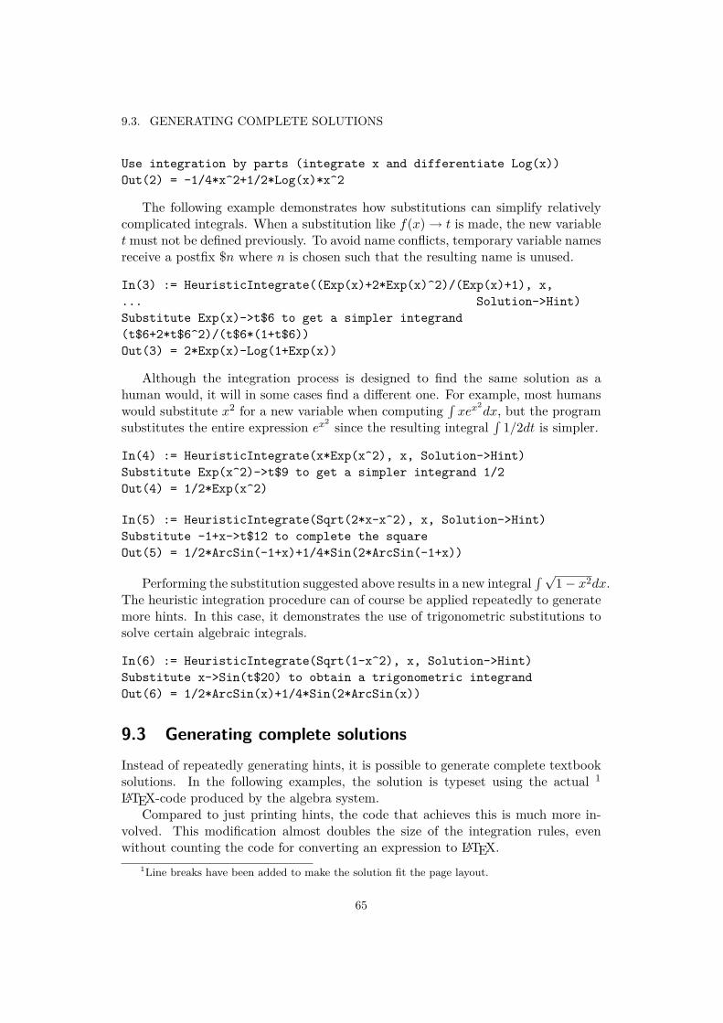
9.3. GENERATING COMPLETE SOLUTIONS

Use integration by parts (integrate x and differentiate Log(x))Out(2) = -1/4*x^2+1/2*Log(x)*x^2

The following example demonstrates how substitutions can simplify relativelycomplicated integrals. When a substitution like f(x)→ t is made, the new variabletmust not be defined previously. To avoid name conflicts, temporary variable namesreceive a postfix $n where n is chosen such that the resulting name is unused.

In(3) := HeuristicIntegrate((Exp(x)+2*Exp(x)^2)/(Exp(x)+1), x,... Solution->Hint)Substitute Exp(x)->t$6 to get a simpler integrand(t$6+2*t$6^2)/(t$6*(1+t$6))Out(3) = 2*Exp(x)-Log(1+Exp(x))

Although the integration process is designed to find the same solution as ahuman would, it will in some cases find a different one. For example, most humanswould substitute x2 for a new variable when computing

∫xex

2dx, but the program

substitutes the entire expression ex2 since the resulting integral∫

1/2dt is simpler.

In(4) := HeuristicIntegrate(x*Exp(x^2), x, Solution->Hint)Substitute Exp(x^2)->t$9 to get a simpler integrand 1/2Out(4) = 1/2*Exp(x^2)

In(5) := HeuristicIntegrate(Sqrt(2*x-x^2), x, Solution->Hint)Substitute -1+x->t$12 to complete the squareOut(5) = 1/2*ArcSin(-1+x)+1/4*Sin(2*ArcSin(-1+x))

Performing the substitution suggested above results in a new integral∫ √

1− x2dx.The heuristic integration procedure can of course be applied repeatedly to generatemore hints. In this case, it demonstrates the use of trigonometric substitutions tosolve certain algebraic integrals.

In(6) := HeuristicIntegrate(Sqrt(1-x^2), x, Solution->Hint)Substitute x->Sin(t$20) to obtain a trigonometric integrandOut(6) = 1/2*ArcSin(x)+1/4*Sin(2*ArcSin(x))

9.3 Generating complete solutionsInstead of repeatedly generating hints, it is possible to generate complete textbooksolutions. In the following examples, the solution is typeset using the actual 1

LATEX-code produced by the algebra system.Compared to just printing hints, the code that achieves this is much more in-

volved. This modification almost doubles the size of the integration rules, evenwithout counting the code for converting an expression to LATEX.

1Line breaks have been added to make the solution fit the page layout.

65

CHAPTER 9. RESULTS

In(1) := HeuristicIntegrate((1+x^2)*Sin(x), x, Solution->TeXForm)

∫sin (x)

(1 + x2

)dx ={

Use integration by parts (integrate sin (x) and differentiate 1 + x2)}

=∫2 cos (x)xdx− cos (x)

(1 + x2

)=

{Use integration by parts (integrate cos (x) and differentiate x)} =

2(−∫

sin (x) dx+ sin (x)x)− cos (x)

(1 + x2

)=

2 (cos (x) + sin (x)x)− cos (x)(1 + x2

)Out(1) = 2*(Cos(x)+Sin(x)*x)-Cos(x)*(1+x^2)

In(2) := HeuristicIntegrate(x*Log(x), x, Solution->TeXForm)

∫log (x)xdx =

{Use integration by parts (integrate x and differentiate log (x) )} =

−∫ 1

2xdx+ 12 log (x)x2 = −1

4x2 + 1

2 log (x)x2

Out(2) = -1/4*x^2+1/2*Log(x)*x^2

In(3) := HeuristicIntegrate((Exp(x)+2*Exp(x)^2)/(Exp(x)+1), x,... Solution->TeXForm)

∫ (exp (x) + 2 exp (x)2

)(1 + exp (x)) dx = {Substitute exp (x) ->t$6} =

∫ (t$6 + 2t$62

)t$6 (1 + t$6) dt$6 = − log (1 + t$6) + 2t$6 =

{Substitute t$6-> exp (x)} = 2 exp (x)− log (1 + exp (x))

Out(3) = 2*Exp(x)-Log(1+Exp(x))

In(4) := HeuristicIntegrate(x*Exp(x^2), x, Solution->TeXForm)

∫exp

(x2)xdx =

{Substitute exp

(x2)->t$9

}=∫ 1

2dt$9 = 12t$9 =

{Substitute t$9-> exp

(x2)}

=12 exp

(x2)

Out(4) = 1/2*Exp(x^2)

66

9.4. INTEGRALS WHICH REMAIN UNEVALUATED

9.4 Integrals which remain unevaluatedAs mentioned several times before, the integration rules does not solve every inte-gral. We will now take a closer look at some of the integrals which fail, and howthe integration rules could be enhanced.Problem The integral ∫

x2 log(1 + x2)dx

is not evaluated.

Solution The natural way to solve this integral is to use integration by parts sinceintegrating x2 and differentiating log(1+x2) will reduce the problem to integrating arational function. This is a straightforward generalization of the rule for integratingP (x) log(x), but it has not been implemented in order to make a fair comparisonof the success rate. (Tweaking the rules to fit a finite evaluation set would ofcourse make the results meaningless as one could in principle add one rule for eachproblem).

Problem The integral ∫ 13√x+√xdx

is not evaluated.

Solution The problem is caused by the fact that there are no rules for handlingmultiple algebraic extensions. In this case, it is easy to see that both radicalscan be expressed in terms of 6

√x. A similar property holds in general since every

finite separable extension has a primitive element. As every extension of a fieldof characteristic 0 is separable, this means that every algebraic extensions we areconsidering can be obtained by adjoining a single element to the base field.

Problem The integral

∫ √1 +

(d

dxlog(1− x2)

)2dx =

∫ √1 +

( −2x1− x2

)2dx

is not evaluated.

Solution This failure is mostly a consequence of insufficient simplification. A goodsimplification algorithm would realize that√

1 +( −2x

1− x2

)2=√

1 + 2x2 + x4

(1− x2)2 =√

(1 + x2)2

(1− x2)2 = 1 + x2

1− x2

which can easily be integrated.

67

CHAPTER 9. RESULTS

When examining the algorithm’s behavior, one notices that most problems arecaused by algebraic integrands. This reinforces our feeling that he algebraic case isthe hardest even with the rule-based approach.

68

Chapter 10

Discussion

10.1 Extensions of Risch’s algorithm

The Risch algorithm as described in the preceding chapters can be extended inseveral ways. The easiest such improvement would be to allow arbitrary primitiveand hyperexponential extensions in the integrand, rather than just logarithms andexponentials.

Definition 10.1 Let E be a differential field extension of F. An element θ ∈ E issaid to be

1. primitive if there exists f ∈ F such that θ′ = f

2. hyperexponential if there exists f ∈ F such that θ′ = fθ

Notice the similarity between the definition of primitive and hyperexponential ex-tensions, and the definitions of logarithmic (4.9) and exponential (4.10) extensions.Because of this similarity, most of the theorems in chapters 5 and 6 will hold forprimitive and hyperexponential extensions with little or no change in the proofs.

It is also possible to modify Risch’s algorithm to handle tangents without rewrit-ing them as complex exponentials. This is done by treating tangents as a third typeof field extension in the absence of imaginary numbers, but come at the cost of anew case in almost all proofs and algorithms in the preceding chapters. Neverthe-less, it could be worth the extra complications since the final output might be morereadable.

Unlike the algorithm presented here, the method originally described by Rischcould also integrate algebraic functions. Actually creating a practical algorithm forthis requires algorithms from algebraic geometry which are beyond the scope of thisthesis.

There are generalizations of Liouville’s theorem which allow certain classes ofspecial functions in the integral, for example by Singer et al. [25] and by Baddoura[1]. These extensions can sometimes be used to compute integrals in terms of

69

CHAPTER 10. DISCUSSION

non-elementary functions, but it is not fully solved how to turn them into efficientdecision procedures.

10.2 Concerning the complexity of integrationThere are many reasons why it is difficult to perform a complexity analysis ofRisch’s algorithm. The first problem is that it is not clear what exactly is meant byRisch’s algorithm. The method described by Risch was an outline of an algorithm,but many subproblems were not satisfactorily solved at the time. Today, Risch’salgorithm is used to denote almost any realization of Risch’s outline for integratingelementary functions, and consequently the complexities can vary.

One major problem is that it is not clear how one should measure the size ofthe input. If one uses the number of bits in the input as a measure, then it is easyto see that even integration of rational functions will have exponential complexitysince

∫ xn−1x−1 dx is a polynomial with n terms while the input size is proportional to

log(n) where n is a large integer. In this case, the swell could be dismissed as anartifact of using a rational expression to represent a polynomial, but similar swelloccur for example when computing

∫xnexdx. Since

∫xnexdx = p(x)ex where p(x)

is a polynomial of degree n with coefficients up to n!, it is easy to see that both thenumber of terms and the bit length of the coefficients grow exponentially with thebit length of n.

Aside from the theoretical difficulties in defining the complexity of Risch’s al-gorithm, there are also practical difficulties when computing it. The most obviousproblem is the sheer number of functions or algorithms that are part of the inte-gration procedure. Because of intermediate expression swell, not only would onehave to analyze the complexity of all the subalgorithms, but also how their outputsize depend on input size. One way to deal with this problem is to use modulartechniques.

Gerhard [15] gave modular algorithms for several of the subproblems needed forintegration, including some asymptotically optimal solutions. For rational functionshe obtained the following simple result.

Theorem 10.2 Let f, g ∈ Z \ {0} be polynomials of degree at most n with integercoefficients bounded by 2λ. Then the symbolic integral of the rational function f/gcan be computed using O(n8 + n6λ2) word operations using classical arithmetic andO(n2M(n3+n2λ) log(nλ)) word operations using fast multiplication with costM(n).

10.3 Future workThere are many aspects of symbolic integration that would be interesting to examinefurther, the most obvious one being how to extend Risch’s algorithm to handle newclasses of functions. Some less ambitious and perhaps less obvious projects arediscussed in the following paragraphs.

70

10.3. FUTURE WORK

10.3.1 A simpler proof of the Lazard-Rioboo-Trager formulaThe Lazard-Rioboo-Trager formula 3.5 for integrating rational functions was leftwithout proof because the known proofs depend on how the subresultants changeunder a homomorphism of the coefficient ring. Resultants and subresultants aretraditionally studied by interpreting them as determinants of certain matrices. Sinceintegration is such a fundamental problem, it would be very nice to be able to explainthe Lazard-Rioboo-Trager theorem without having to include this extra machinery.This motivates asking whether the theorem can be proven directly using the samedefinition and approach as in appendix C.

10.3.2 Symbolic integration in numerical computationsSymbolic algorithms are often perceived as rather restricted, compared to its nu-merical counterparts. While it is true that many problems cannot be solved sat-isfactorily using only algebraic manipulation, the numerical algorithms also havea number of weaknesses related to round-off and truncation errors. In particular,one will not know whether the computed solution even resemble the exact solutionwithout some form of precision tracking or analysis of how the numerical errorspropagate in the algorithm. Although numerical computation was not the subjectof this thesis, it would be interesting to know the extent to which symbolic algo-rithms can be used to automatically transform problems to forms which are moresuitable for numerical computation.

Davenport [9] did a small informal study of how well symbolic integration worksin practice based on problems suggested by colleagues. Of the problems considered,he found that approximately one third could be solved by symbolic integration,another third was simplified (for example by solving one dimension of a multipleintegral) while the remaining third did not yield to a symbolic approach.

Geddes and Fee [13] discussed the use of symbolic techniques to remove singu-larities in numerical integrals, a method which is used internally by Maple. Theauthors also remarked that their experiences with hybrid symbolic-numeric algo-rithms had been very promising.

With some exceptions like the ones mentioned above, there seem to be littlework published on how to combine computer algebra with numerical computationsand definitely less than the amount published on either subject.

10.3.3 Symbolic integration in educationThe heuristic method discussed in chapter 2 can be adapted in a number of waysthat might be useful in education. For example it could:

• Provide hints on how to compute an integral

• Provide complete solutions

• Generate examples that demonstrate the use of a certain rule

71

CHAPTER 10. DISCUSSION

• Generate exercises that can be solved using a certain set of rules

The feasibility of generating hints and complete solutions was demonstrated in sec-tions 9.2 and 9.3, but it seems that neither these nor the other possibilities havebeen implemented in the existing computer algebra systems.

The tasks listed above are traditionally done by the teacher or the author of thecourse book, but could be done interactively by a computer algebra system. Theability to automatize these asks could be utilized for example to create programswhich generates exercises depending on the which rules the student has previouslyhad difficulties applying. If the students get stuck, they could obtain instant feed-back by asking the program for hints or solutions. In addition, a computer algebrasystem would typically choose rules in a more systematic way than most humans,which may may make easier to memorize the rules and how they are applied.

It is, however, difficult to predict whether the use of algebra systems wouldreally improve learning in calculus courses. The availability of programs that cando the integrals for them, may make the students more inclined to cheat, or makethem perceive the exercises as pointless. The risk of cheating on homeworks can beto some degree be allayed by choosing problems which are either not handled wellor handled differently by the integration rules compared to what a human would.In section 9.2 we saw that that xex2 is an example of such a problem.

Thus, before any serious use in education one would have to investigate whetheror not the computer algebra improves learning and, if so, how it should be incorpo-rated into the curriculum.

10.3.4 Improvements of the implementation

From a practical perspective, it would have been very nice to implement Risch-Norman’s algorithm. Bronstein has shown that it can be implemented in Maple inless than 100 lines of code [2], and that it performs very well in practice. Just asthe major difficulty in implementing heuristic integration is the pattern matching,the major difficulty in implementing Risch-Norman’s parallel integration algorithmis the need for factorization of multivariate polynomials, possibly over algebraicnumber fields. Since our main goal when writing the computer algebra system wasto implement the heuristic integration rules, the design choices have favored thisapproach. No time was spent on developing the advanced polynomial algorithmsthat are prerequisites for Risch-Norman’s algorithm.

10.4 Conclusions

There are several approaches to symbolic integration with different strengths andweaknesses. A set of heuristic integration rules is easy to understand and can beimproved by the user when the need arise. On the other hand, the success rate ismoderate, typically similar to that of a decent student. The most interesting aspect

72

10.4. CONCLUSIONS

of this approach is its ability to generate readable solutions, demonstrated in section9.3.

The Risch-Norman algorithm is a more systematic approach which offer a highrate of success and can even be applied to non-elementary integrands. Since thealgorithm simply does an educated guess of the general form of the integral, differ-entiates it and then tries to identify the coefficients, it is not very difficult to un-derstand the idea or verify its correctness. However, understanding why the guessis made in a particular way requires some differential algebra. Implementations ofthe algorithm can be short, but requires several algorithms from computer algebrasuch as equivalence testing, solution of linear systems and multivariate polynomialfactorization.

Being entirely based on differential algebra, the Risch decision procedure is themost difficult to understand of the three discussed methods. It is also the mostdifficult to implement as it consists of many parts not normally used elsewhere ina computer algebra system. The advantage of this method is that it will find anelementary integral of an elementary function if one exists and otherwise detectthat the integral in non-elementary. Thus, the success rate is the best possible inthe context of elementary functions, but on the other hand, it cannot easily be gen-eralized to handle non-elementary functions. Except for special applications wheredetection of non-elementary integrals is necessary, it would be better to implementRisch-Norman’s algorithm instead of the full Risch algorithm.

73

Bibliography

[1] J. Baddoura. Integration in finite terms with elementary functions and dilog-arithms. J. Symb. Comput., 41(8):909–942, 2006.

[2] M. Bronstein. The poor man’s integrator, v 1.1, 2005. Available online fromhttp://www-sop.inria.fr/cafe/Manuel.Bronstein/pmint/pmint.txt(Retrieved October 20, 2008).

[3] M. Bronstein. The transcendental Risch differential equation. J. Symb. Com-put., 9(1):49–60, 1990.

[4] M. Bronstein. Symbolic integration. I: Transcendental functions, volume 1 ofAlgorithms and Computation in Mathematics. Springer-Verlag, Berlin, secondedition, 2005.

[5] M. Bronstein. Structure theorems for parallel integration. J. Symb. Comput.,42(7):757–769, 2007.

[6] W. S. Brown. The subresultant PRS algorithm. ACM Trans. Math. Software,4(3):237–249, 1978.

[7] H. Cohen. A course in computational algebraic number theory, volume 138 ofGraduate Texts in Mathematics. Springer-Verlag, Berlin, 1993.

[8] J. S. Cohen. Computer algebra and symbolic computation: Mathematical meth-ods. AK Peters Ltd., Natick, Massachusetts, 2003.

[9] J. H. Davenport. Symbolic and numeric manipulation of integrals. In AccurateScientific Computations, pages 168–180. Springer-Verlag, 1985.

[10] J. H. Davenport, Y. Siret, and E. Tournier. Computer algebra: Systems andalgorithms for algebraic computation. Academic Press Ltd., London, secondedition, 1993.

[11] J. B. Fraleigh. A first course in abstract algebra. Addison-Wesley PublishingCompany, Inc, 1999.

[12] K. O. Geddes, S. R. Czapor, and G. Labahn. Algorithms for computer algebra.Kluwer Academic Publishers, Boston, MA, 1992.

75

BIBLIOGRAPHY

[13] K. O. Geddes and G. J. Fee. Hybrid symbolic-numeric integration in MAPLE.In ISSAC, pages 36–41, 1992.

[14] K. O. Geddes and L. Y. Stefanus. On the Risch-Norman integration methodand its implementation in MAPLE. In ISSAC ’89: Proceedings of the ACM-SIGSAM 1989 international symposium on Symbolic and algebraic computa-tion, pages 212–217, New York, NY, USA, 1989. ACM.

[15] J. Gerhard. Modular Algorithms in Symbolic Summation and Symbolic Inte-gration, volume 3218 of Lecture Notes in Computer Science. Springer, 2004.

[16] G. H. Hardy. The integration of functions of a single variable. Hafner Pub-lishing Co., New York, 1971. Reprint of the second edition, 1916, CambridgeTracts in Mathematics and Mathematical Physics, No. 2.

[17] S. Lang. Algebra, volume 211 of Graduate Texts in Mathematics. Springer-Verlag, New York, third edition, 2002.

[18] D. Lazard and R. Rioboo. Integration of rational functions: rational computa-tion of the logarithmic part. J. Symb. Comput., 9(2):113–115, 1990.

[19] R. E. Maeder. Algbench: An object-oriented symbolic core system. LectureNotes in Computer Science, 721:56–64, 1993.

[20] K. McIsaac. Pattern matching algebraic identities. SIGSAM Bull., 19(2):4–13,1985.

[21] J. Moses. Algebraic simplification: a guide for the perplexed. In SYMSAC’71: Proceedings of the second ACM symposium on Symbolic and algebraicmanipulation, pages 282–304, New York, NY, USA, 1971. ACM.

[22] T. Mulders. A note on subresultants and the Lazard/Rioboo/Trager formulain rational function integration. J. Symb. Comput., 24(1):45–50, 1997.

[23] D. Richardson. Some undecidable problems involving elementary functions ofa real variable. J. Symbolic Logic, 33(4):514–520, 1968.

[24] R. H. Risch. The problem of integration in finite terms. Trans. Amer. Math.Soc., 139:167–189, 1969.

[25] M. F. Singer, B. D. Saunders, and B. F. Caviness. An extension of Liouville’stheorem on integration in finite terms. In Proc. 1981 ACM Symposium onSymbolic and Algebraic Computation, 1981.

[26] B. L. van der Waerden. Modern Algebra. Vol. I. Frederick Ungar PublishingCo., New York, N. Y., 1949.

[27] S. Wolfram. The Mathematica Book, Fifth Edition. Wolfram Media, 2003.

76

Appendix A

Partial fractions decomposition

In this appendix, we prove the existence of a partial fraction decomposition.

Lemma A.1 Let F be a field and p/(qr) a proper rational expression with p, q, r ∈F[x] and q, r relatively prime. Then there exists polynomials a, b ∈ F[x] such that

p

qr= a

q+ b

r

where deg(a) < deg(q) and deg(b) < deg(r)

Proof The condition that q and r are relatively prime means that gcd(q, r) = 1,so there exist polynomials a and b such that ar + bq = 1. Hence,

p

qr= p(ar + bq)

qr= pa

q+ pb

r

In this expression however, pa and pb need not have degrees less than deg(q) anddeg(r) respectively. Using the division algorithm, we obtain pa = daq + a andpb = dbr + b. Now, for

p

qr= daq + a

q+ dbr + b

r= (da + db)qr + ar + bq

qr

to be a proper fraction, we need da + db = 0. Without loss of generality, we mayassume that da = db = 0, so

p

qr= a

q+ b

r

as desired. �

Theorem A.2 Let F be a field and p/q a proper rational expression with p, q ∈ F[x]and suppose that q has the factorization q = ∏k

i=1 qeii where the qi are pairwise

relatively prime. Then there exists polynomials rij ∈ F[x] such that

p

q=

k∑i=1

ei∑j=1

rij

qji

77

APPENDIX A. PARTIAL FRACTIONS DECOMPOSITION

where deg(rij) < deg(qi)

Proof Using the previous lemma k−1 times gives a partial fraction decomposition

p

q=

k∑i=1

riqii

where deg(ri) < deg(qii). If deg(ri) ≥ deg(qi), euclidean division can express ri =riqi + rij , so

ri

qji= rij

qji+ ri

qj−1i

where deg(rij) < deg(qi) and deg(ri) < deg(qj−1i ). Induction on j proves the

theorem. �

78

Appendix B

Square-free factorization

Definition B.1 A polynomial is square-free if it has no repeated factors.

Theorem B.2 A polynomial p ∈ F[x] is square-free if and only if gcd(p, p′) = 1.

Proof (⇐) Assume that p has some repeated factor, so p = fnh for some n > 1.Then p′ = nfn−1f ′h+ fnh′, so p and p′ have a common factor fn−1.(⇒) On the other hand, if p is square-free, with irreducible factorization

p = p1p2 · · · pk

where all pi are distinct, then

p′ = p′1p2 · · · pk + p1p′2p3 · · · pk + . . .+ p1p2 · · · pk−1p

′k

Now, any nontrivial divisor of p must be a multiple of some pi, so if gcd(p, p′) isnontrivial we can assume that pi divides both p and p′. Since pi clearly divides allterms of p′ except the first, it must also divide p′i in order to divide p′. This is acontradiction since deg(pi) > deg(p′i), so gcd(p, p′) must be 1. �

Definition B.3 A square-free factorization of p is a factorization p = ∏ki=0(pi)i,

such that all pi are square-free and gcd(pi, pj) = 1 if i 6= j.

While it is difficult to compute the full factorization into irreducibles, computinga square-free factorization is not.

Let p ∈ F[x] have the square-free factorization p = p1p22p

33 · · · pkk, so

p′ =k∑i=1

(i− 1)pi−1i p′i

∏i 6=j

pjj

Let

a1 = gcd(p, p′) = p2p23p

34 · · · pk−1

k

79

APPENDIX B. SQUARE-FREE FACTORIZATION

andb1 = p

gcd(p, p′) = p1p2p3 · · · pk

Now we can iterate

ci = gcd(ai, bi) = pi+1pi+2 · · · pkai+1 = ai

ci= pi+2p

2i+3 · · · pk−i−1

k

bi+1 = ci

The square-free factors pi are given by pi = bici.

Theorem B.4 If F has characteristic 0, then a square-free factorization over Fis simultaneously a square-free factorization over F, where F denotes the algebraicclosure of F.

Proof This classic result in field theory is usually stated by saying that all fieldsof characteristic 0 are perfect. The theorem and its proof can be found in mostabstract algebra textbooks, for example Fraleigh’s [11] and van der Waerden’s [26].�

It is interesting that this holds for all finite fields too, so the only fields for whicha square-free factorization over F can fail to be a square-free factorization over F areinfinite fields of prime characteristic. Such fields are not very common in practice.

80

Appendix C

Greatest common divisors and theresultant

If F is a field, then F[x] is an euclidean domain i.e. an integral domain with euclideandivision. It is well known that the euclidean algorithm can be used to computegreatest common divisors in any euclidean domain. For any unique factorizationdomain D, D[x] will be also be a unique factorization domain, but it need not beeuclidean because we cannot divide by the coefficients. In practice, this happensfor polynomials over Z and for polynomials in several variables over any field.

Since we cannot use the familiar euclidean algorithm to compute greatest com-mon divisors, we will define a pseudo-division which share some important prop-erties with the ordinary polynomial division, but which can be computed withoutdivisions in the coefficient ring.

Definition C.1 Let a, b ∈ D[x] be polynomials over a unique factorization domainD and let lc(b) denote the leading coefficient of b. Then there are polynomialsq, r ∈ D[x] such that

lc(b)deg(a)−deg(b)+1a = qb+ r

and deg(r) < deg(b). We call q = pquo(a, b) the pseudo-quotient and r = prem(a, b)the pseudo-remainder of a and b.

Definition C.2 Let D be a unique factorization domain, and let p = ∑ni=0 pix

i bea polynomial in D[x]. We define the content and primitive part of p as

cont(p) = gcd(p0, p1, . . . , pn)pp(p) = p/ cont(p)

Definition C.3 Let D be a unique factorization domain, and p, q polynomials inD[x] with deg(p) ≥ deg(q). We define the polynomial remainder sequence or PRS

81

APPENDIX C. GREATEST COMMON DIVISORS AND THE RESULTANT

for p and q as the finite sequence defined by

R0 = p(x)R1 = q(x)

βiRi+1 = prem(Ri−1, Ri) if Ri 6= 0

where βi is chosen to limit coefficient growth. The particular PRS with βi = 1 iscalled the euclidean PRS and the one with βi = cont(prem(Ri−1, Ri)) is called theprimitive PRS.

Definition C.4 The polynomials p and q in D[x] are said to be similar if thereexist a, b ∈ D\{0} such that ap = bq

Theorem C.5 If p and q are polynomials in D[x] where D is a unique factorizationdomain and (R0, R1, . . . , Rk, 0) a PRS for p and q, then gcd(p, q) is similar to Rk.Furthermore, if p and q are primitive, then

gcd(p, q) = pp(Rk)

Proof Inserting the definition of the pseudo-remainder in the definition of the PRSwe see that there exist α, β ∈ D and Q ∈ D[x] such that

αRi−1 = QRi + βRi+1

Hence

α gcd(Ri−1, Ri) = gcd(αRi−1, Ri) = gcd(Ri, βRi+1) = β gcd(Ri, Ri+1)

and iterating this, we see that there are elements a, b ∈ D such that

a gcd(p, q) = b gcd(Rk, 0) = bRk

which proves the first part of the statement. If p and q are primitive then pp(gcd(p, q)) =gcd(p, q) so

gcd(p, q) = pp(gcd(p, q)) = pp(a gcd(p, q)) = pp(bRk) = pp(Rk)

�

This last theorem shows how to use polynomial remainder sequences to computegreatest common divisors. We will now turn the attention to the resultant and itsrelationship with the greatest common divisor.

Definition C.6 Let D be an integral domain, and let p and q be polynomials inD[x], with factorizations

p(x) = am∏i=1

(x− αi)

q(x) = bn∏j=1

(x− βj)

82

in D[x]. We define the resultant with respect to x as

resx(p, q) = anbmm∏i=1

n∏j=1

(αi − βj)

= anm∏i=1

q(αi)

= (−1)mnbmn∏j=1

p(βj)

We will not prove the equivalence of the three expressions above, nor that theseemingly unnecessary multiplications by an and bm in fact ensure that resx(p, q) ∈D. The interested reader can consult almost any algebra textbook (for example[17]) for a discussion of the mathematical foundations of the resultant, and [6] or [7]for nice descriptions of the subresultant algorithm for computing resultants. Whenthere can be no confusion about the variable, we omit the explicit reference to itand write res(p, q) instead of resx(p, q).

Theorem C.7 Let D be a unique factorization domain, and p, q polynomials inD[x]. Then

resx(p, q) = 0 ⇐⇒ deg(gcd(p, q)) > 0

Proof (⇐) Suppose that deg(gcd(p, q)) > 0. Then p and q have a common zero,so resx(p, q) = anbm

∏mi=1

∏nj=1 (αi − βj) = 0.

(⇒) On the other hand, suppose that resx(p, q) = anbm∏mi=1

∏nj=1 (αi − βj) = 0.

Since D is an integral domain, one of the factors αi − βj must be zero, so p and qhave a common root and thus deg(gcd(p, q)) > 0. �

Definition C.8 The subresultant polynomial remainder sequence for the polynomi-als p, q ∈ D[x] is the PRS defined by βi = gi−1h

δi−1i−1 where

di = deg(Ri)δi = di − di+1

g0 = h0 = 1gi = lc(Ri)

hi = gδi−1i h

1−δi−1i−1

The subresultant PRS can be used to compute greatest common divisors and,as we shall see, resultants. The following elegant proof is essentially from Cohen[7].

83

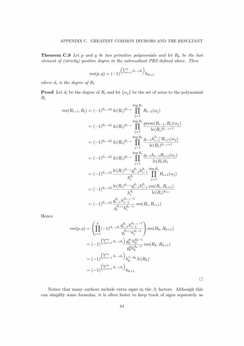
APPENDIX C. GREATEST COMMON DIVISORS AND THE RESULTANT

Theorem C.9 Let p and q be two primitive polynomials and let Rk be the lastelement of (strictly) positive degree in the subresultant PRS defined above. Then

res(p, q) = (−1)(∑k

i=1 di−1di

)hk+1

where di is the degree of Ri

Proof Let di be the degree of Ri and let {αj} be the set of zeros to the polynomialRi

res(Ri−1, Ri) = (−1)di−1di lc(Ri)di−1degRi∏j=1

Ri−1(αj)

= (−1)di−1di lc(Ri)di−1degRi∏j=1

prem(Ri−1, Ri)(αj)lc(Ri)δi−1+1


gi−1hδi−1i−1 Ri+1(αj)

lc(Ri)δi−1+1


gi−1hi−1Ri+1(αj)lc(Ri)hi

= (−1)di−1dilc(Ri)δi−1gdii−1h

dii−1

hdii

degRi∏j=1

Ri+1(αj)

= (−1)di−1dilc(Ri)δi−1gdii−1h

dii−1

hdii

res(Ri, Ri+1)lc(Ri)di+1

= (−1)di−1digdii−1h

di−1−1i−1

gdi+1i hdi−1

i

res(Ri, Ri+1)

Hence

res(p, q) =

k∏i=1

(−1)di−1digdii−1h

di−1−1i−1

gdi+1i hdi−1

i

res(Rk, Rk+1)

= (−1)(∑k

i=1 di−1di

)gd1

0 hd0−10

g0kh

dk−1k

res(Rk, Rk+1)

= (−1)(∑k

i=1 di−1di

)h1−dkk lc(Rk)

= (−1)(∑k

i=1 di−1di

)hk+1

�

Notice that many authors include extra signs in the βi factors. Although thiscan simplify some formulas, it is often faster to keep track of signs separately as

84

we did above. Since the purpose of the βi is to limit coefficient growth, it does notreally matter which convention one uses.

85

Date post:	03-Feb-2022
Category:	Documents
Upload:	others
View:	1 times
Download:	0 times

Symbolic Integration - KTH

Documents