To improve the test generation performance using SAT-based BMC [1], Chap. 5described several efficient test generation techniques using clustering and learningtechniques. In this approach, checking the first (base) property can be a major bot-tleneck during the test generation, because the base property cannot actively obtainlearnings from others to improve its test generation time. Especially when checkinga large design with complex properties [i.e., properties with large cone of influ-ence (COI) or deep bounds], BMC-based methods are very costly since large SATinstances indicate long SAT search time.
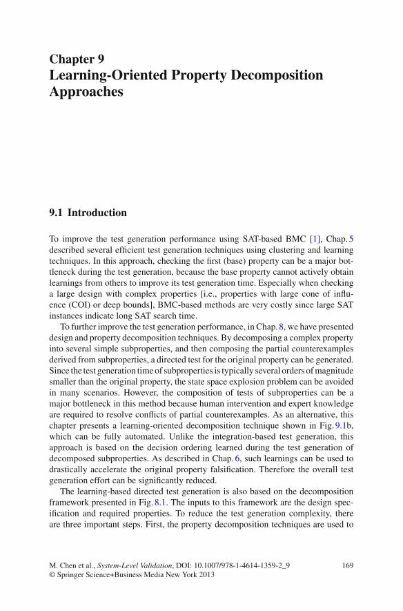
To further improve the test generation performance, in Chap. 8, we have presenteddesign and property decomposition techniques. By decomposing a complex propertyinto several simple subproperties, and then composing the partial counterexamplesderived from subproperties, a directed test for the original property can be generated.Since the test generation time of subproperties is typically several orders of magnitudesmaller than the original property, the state space explosion problem can be avoidedin many scenarios. However, the composition of tests of subproperties can be amajor bottleneck in this method because human intervention and expert knowledgeare required to resolve conflicts of partial counterexamples. As an alternative, thischapter presents a learning-oriented decomposition technique shown in Fig. 9.1b,which can be fully automated. Unlike the integration-based test generation, thisapproach is based on the decision ordering learned during the test generation ofdecomposed subproperties. As described in Chap. 6, such learnings can be used todrastically accelerate the original property falsification. Therefore the overall testgeneration effort can be significantly reduced.
The learning-based directed test generation is also based on the decompositionframework presented in Fig. 8.1. The inputs to this framework are the design spec-ification and required properties. To reduce the test generation complexity, thereare three important steps. First, the property decomposition techniques are used to
Fig. 9.1 Two property decomposition techniques. a Integration-based decomposition, b Learning-oriented decomposition
reduce the complexity during property falsification. Next, by checking the selectedprofitable subproperties, we can collect useful learnings for the original propertychecking. Finally, the learned knowledge (i.e., decision ordering) can be utilized toavoid the unnecessary conflicts during the original test generation. Therefore, thetest generation time can be drastically reduced.
The rest of the chapter is organized as follows. Section 9.2 presents the relatedwork on decomposition as well as learning techniques. Section 9.3 proposes twonovel property decomposition methods based on learning techniques. Section 9.4presents the decision ordering based learning techniques for original property check-ing. Section 9.5 describes how to utilize the learned knowledge from the decomposedproperties for test generation. Section 9.7 presents case studies using both hardwareand software designs. Finally, Sect. 9.8 summarizes the chapter.
9.2 Related Work
To overcome the complexity issues during design and verification, various decompo-sition techniques have been proposed. Case et al observed that some signals get fixedto constant values after some time frames [2]. They presented automated techniques todetect and eliminate redundancy related to transient signals and initialization inputs,which enable verification efficiencies in terms of logic reduction. Lin et al. [3] pro-posed a new formulation of Ashenhurst decomposition based on SAT solving. It canefficiently decompose a Boolean function into a network of smaller sub-functions.However, this method is mainly used in logic synthesis. As described in Chap. 8,although Koo et al. [4] presented a promising design and property decompositionmethod for test generation, it is hard to automate the composition of generated partialtests corresponding to the decomposed properties.
Sharing learnings across properties can improve overall performance since therepeated validation efforts can be avoided. Due to the commonality between differ-ent SAT instances of a property, Strichman [5] found that the conflict clauses canbe replicated and forwarded as a constraint. Based on this observation, incrementalSAT solvers [5, 6] are developed to reuse the learned conflict clauses from lowerbound SAT instances to prune the SAT search for larger bound SAT instances. In[7], Chen and Mishra noticed that when checking a large set of relevant properties,SAT instances of similar properties have a large overlap of CNF clauses and canbe clustered (described in Chap. 5). A large number of conflict clauses generated bya base property can be forwarded to other properties in the cluster. As an alterna-tive of conflict clause forwarding, decision ordering heuristics [8] can be used asanother learning to improve the SAT searching. In [9], Strichman presented an BMCoptimization based on decision ordering by exploiting the characteristics of BMCformulas. Wang et al. [10] analyzed the correlation among different SAT instancesof a property. They used the unsatisfiable core of previously checked SAT instancesto guide the variable ordering for the current SAT instance. When checking a set ofsimilar properties, Chen et al. [11] tuned the decision ordering of the current propertybased on the decision ordering results of the previously checked properties (describedin Chap. 6). By sharing learnings (i.e., conflict clauses or decision ordering) amongproperties, the overall test generation time can be reduced. However, these learningtechniques do not consider how to actively learn from other simpler properties. Forexample, when sharing learnings among a cluster of similar properties, checking thefirst property will be a major bottleneck because there is no knowledge that can belearned.
In contrast to conventional methods using learnings, the approach [12] presentedin this chapter is the first attempt to use decision ordering based learning in propertydecomposition to enable automated test generation.
9.3 Learning-Oriented Property Decomposition
This chapter focuses on efficient falsification of safety linear temporal logic (LTL[13]) properties which consist of temporal operators (F, G, X, U) and Boolean con-nectives (∧,∨,¬ and →). The basic idea is to utilize the learnings from simpleproperties for complex property checking.
9.3.1 Spatial Property Decomposition
For a complex property which involves multiple components of the design, it canbe partitioned into multiple component-level subformulas. For example, a complexsystem-level property P can be broken into 2 subproperties P1 and P2 with differentCOI. Assuming that P1 has a smaller COI than P , it usually needs less time and space
than that of checking the complex property P . If the partial counterexample generatedby P1 can be refined to guide the complex property falsification, the original propertyis spatially decomposable.
Definition 9.1 A false property P in conjunctive form p1 ∧ p2 ∧ . . . ∧ pn or indisjunctive form p1 ∨ p2 ∨ . . . ∨ pn is spatially decomposable if all of the followingconditions are satisfied.
• If the decomposed properties are in the form p1 ∧ p2 ∧ . . . ∧ pn , then at least oneproperty pi (1 ≤ i ≤ n) has a counterexample. In this case, the bound of P is theminimum bound of pi which has a counterexample.
• If the decomposed properties are in the form p1 ∨ p2 ∨ . . .∨ pn , then each propertypi (1 ≤ i ≤ n) has a counterexample. In this case, the bound of P is the maximumbound of all decomposed properties.
• The counterexamples generated from properties pi (1 ≤ i ≤ n) can guide the testgeneration for property P . �
According to Definition 9.1, the following rules can be used for complex propertydecomposition.
¬X (p ∨ q) ≡ ¬X (p) ∧ ¬X (q)
¬X (p ∧ q) ≡ ¬X (p) ∨ ¬X (q) (9.1)
¬F(p ∨ q) ≡ ¬F(p) ∧ ¬F(q)
The property in the form of ¬F(p ∧ q) and ¬F(p → q) cannot be directlydecomposed into conjunctive or disjunctive form. However, by introducing a clockclk for synchronization, they can be spatially decomposed (see the proof in Lemma8.6). It is important to note that the value of the clk indicates the bound of the falseproperty. Equation (9.2) shows that the counterexample of ¬F(p ∧q ∧ clk = k) canbe refined by the counterexamples of ¬F(p ∧ clk = k) and ¬F(q ∧ clk = k).
For a property in the form F(p → q), p describes the precondition and q indicatesthe postcondition. When G(¬p) holds, F(p → q) will be vacuously true, andthe checking of ¬F(p → q) will report a counterexample without satisfying theprecondition p. This counterexample may not match the original intention. Equation9.3 shows that the properties in the form of ¬F(p → q∧clk = k) can be transformedinto ¬F(p∧q ∧clk = k) for test generation. The spatial decomposition in Eqs. (9.2)and (9.3) are similar.
¬F(p → q ∧ clk = k) ≡ ¬F(p ∧ q ∧ clk = k)
≡ ¬F(p ∧ clk = k) ∨ ¬F(q ∧ clk = k) (9.3)
where ¬F(p → q ∧ clk = k) and ¬F(p ∧ clk = k) are false.
9.3 Learning-Oriented Property Decomposition 173
Equations (9.1)–(9.3) present several kinds of widely used properties which can bespatially decomposed. In fact, if a complex property can be decomposed in con-junctive form, it needs to sort the subproperties according to their bounds, and checkthem from the smallest to the largest bounds. The counterexample of the first falsifiedproperty can be used as a counterexample for the complex property.
When checking a complex property which can be decomposed in disjunctiveform, it is not necessary to check all its subproperties. This is because, if the COI ofa subproperty is similar to the original property, the complexity of such subpropertywill be similar to the complex property. In this case, it is not economical to uselearning. Therefore, it needs to figure out subproperties with smaller COI than thecomplex property.
According to the commutative law and associative law, for a complex prop-erty, we can classify its atomic subproperties into several clusters. For example, inEq. 9.4, pi and pk are clustered together, and p j belongs to another cluster.
pi ∨ p j ∨ pk = (pi ∨ pk) ∨ p j (9.4)
For each cluster, we generate a refined property which represents all the atomicsubproperties in the cluster to derive the learning. The following clustering rulesbased on experience work well for most of the time: (1) in each cluster, all thevariables in the subformulas should come from the same component (e.g., fetchmodule in a processor); (2) in each cluster, all the subformulas should describe therelated functional scenarios (e.g., fetching instructions and/or data in a processor).
Algorithm 1 outlines the spatial decomposition method which can derive a set ofrefined subproperties with small COI for learning. The inputs of the algorithm area design model D and a complex property P in disjunctive form. Step 1 initializesthe SD_props with an empty set. Step 2 tunes subproperties’ order according tothe commutative law and clusters subproperties using the similarity rules. Step 3selects the ith cluster. If the COI of such cluster is smaller than k
n of P ′s COI,step 4 will generate a new refined property newP for the ith cluster. Step 5 addsnewP to SD_props. The refined property newP for learning represents a cluster ofsubproperties as shown in step 3. Finally, this algorithm will return a set of refinedsubproperties for deriving learnings (described in Sect. 9.4). Since the COI of arefined property in SD_props is small, its test generation time will be much smallerthan that of the original complex property. It is important to note that this algorithmmay return an empty set which means that it is not beneficial or impossible to spatiallydecompose the complex property.
Algorithm 1: Spatial DecompositionInput: i) The design model, D
ii) A property P in the form p1 ∨ p2 ∨ . . . ∨ pn
Output: A set of refined subproperties for learning, SD_props1. SD_props = {};2. (cluster1, . . . , clusterm) = clustering(P, modular/ f unctional);for i is from 1 to m do
3. cluster_i = {prop1, . . . , propk};if C O I (clusteri ) ≤ k
n C O I (P) then4. generate a refined property newP for the clusteri ;5. SD_props = SD_props
⋃newP;
endendreturn SD_props
9.3.2 Temporal Property Decomposition
To eclipse the bound effect, one intuitive way is to deduce a long bound property froma sequence of short bound properties. For example, P1, P2, and P3 (P3 = P) areproperties indicating three different stages of property P . Their bounds are K 1, K 2,and K 3, respectively, and K 1 < K 2 < K 3. Because P1’s counterexample is similarto the prefix of the P2’s counterexample, P1’s counterexample contains rich knowl-edge that can be used when checking P2. Similarly, during the property checking,P3 can benefit from P2. Therefore we can quickly obtain the counterexample (test)for property P . If the counterexamples of lower bound properties can be used toreason about P , the property P is temporally decomposable.
Definition 9.2 A false safety property P is temporally decomposable if all the fol-lowing conditions are satisfied.
• P can be divided into false properties p1, p2, . . . and pn (P = pn) with increasingbounds.
• ¬pi → ¬pi+1 (1 ≤ i ≤ kn − 1), which indicates that the counterexamplegenerated from properties pi can guide the test generation for property pi+1. �
In temporal decomposition, finding the implication relation (“→”) between prop-erties is a key process. In the framework developed by [12], such implication rela-tions are constructed by exploring the order between events, which are described byproperties indicating different stages of the execution. Generally, a system behaviorconsists of a sequence of strongly relevant events. For example, in Fig. 9.2, thereare 9 events. We classify the relation between these events in two categories. Thecause–effect relation (marked by ⇒) defines the relation of consequent events. Forexample, if e1 happens, then e2 should happen in the next stage. The happen before
9.3 Learning-Oriented Property Decomposition 175
Event Happen beforeCause effect
e3 e5e4
e1 e2 e7 e8 e91
3
1 2
22 155
e6
Fig. 9.2 A DAG of event relation
relation (marked by ≺) specifies the relation of conditional events. It indicates whichevents may happen before other events under some condition. For example, e2 ≺ e3means e2 may happen before e3.
During test generation, properties in the form of ¬F(e) are used to indicate that theevent e cannot be activated. According to definition 2, the “⇒” relation can be usedto derive helpful learnings. For example, in Fig. 9.2, let property P1 = ¬F(e1) andproperty P2 = ¬F(e2). Since e1 ⇒ e2 implies F(e1) → F(e2), i.e., ¬P1 → ¬P2,it shows that P1’s counterexample will be helpful for deriving P2’s counterexample.Such information can be used as a learning. The “≺” relation can also be used toindicate the learning information. Assuming e2 ≺ e3, the counterexample of ¬F(e2)
is shorter than the counterexample of ¬F(e3). However, the counterexample of¬F(e2) may have a large overlap of variable assignments with the counterexampleof ¬F(e3). Therefore, the learning from ¬F(e2) can benefit the test generation of¬F(e3).
When checking a large bound property for a transaction, there may be many eventsalong the path to target events. Checking all these events to obtain learnings is time-consuming. For example, assuming that we want to check the property ¬F(e9), therelation between events is described using a directed acyclic graph (DAG) shown inFig. 9.2. Each node indicates an event, and each directed edge indicates the relationof “⇒” or “≺”, and each edge is associated with the delay between events. In thisDAG, there are eight events that happen before e9. However, it is not necessary tocheck all of them.
Since the branch nodes of a DAG indicate critical variable assignment information,it only needs to consider the events which determine the branches along the path frominitial state e1 to the target state e9.
Algorithm 2: Temporal DecompositionInput: i) An event DAG, D
ii) Initial event src, target event destOutput: A property sequence T D_props1. path = Dijkstra(D, src, dest) to find the shortest delay path;2. T D_props = (property for src);for i is from 2 to len (number of events in path) do
3. (ei−1, ei ) = (i − 1)th edge of path;if out_degree(ei−1) + in_degree(ei ) > 2 then
4. Append the property for ei to T D_events;end
endreturn T D_props
Algorithm 2 describes how to obtain a sequence of properties based on temporaldecomposition. It accepts an event DAG with the initial and target events as inputs.Step 1 uses Dijkstra’s algorithm [14] to find a shortest path. Step 2 initializes thesequence TD_props with a property for the initial event. Steps 3 and 4 select thebranch events and append their corresponding properties to the TD_props. Finallythe algorithm reports the property sequence for deriving learnings. By using thisalgorithm, (¬F(e1), ¬F(e3), ¬F(e7)) is a property sequence from the temporaldecomposition in Fig. 9.2.
9.4 Decision Ordering Based Learning Techniques
SAT-based BMC encodes a property checking problem into a SAT instance(a Boolean formula). A counterexample of the property is a satisfying variable assign-ment for this formula. Although the variable assignment of counterexamples derivedfrom the decomposed subproperties may not satisfy the SAT instance of the complexproperty, it has a large overlap with the complex property on the variable assign-ment. Such information can be used as a learning to bias the decision ordering whenchecking the complex property.
During the SAT search, decision ordering plays an important role to quickly finda satisfying assignment. The learning approach presented in this chapter is based onvariable state-independent decaying sum (VSIDS) method [15]. A major differenceis that this learning method incorporates the statistics of decomposed properties.Since different subproperties have different bounds, such information needs to beconsidered in the learning heuristics.
Let bounds be an array which stores the bound of k subproperties. Because in spa-tial method the decomposed subproperties can be independent, the learning betweensubproperties is not significant. So we set bounds[i] = 1(1 ≤ i ≤ k). However,for temporal decomposition, the vstat information (introduced later) of lower bound
9.4 Decision Ordering Based Learning Techniques 177
a
bb
c c c c
a
b
c
b
c c c
0 0
0 0 0 0
0 0
Initialization
0 1
0 0 1 0
0 0 0 0 0 0 0 0 0 0 0 1 0 0
p1: a=0, b=1, c=0
0
a
b
0
c
0
c
000 0
b
c00
c
12
3
3 0
learning: a=0, b=1, c=0
p2: a=0, b=1, c=1
a
c
b b
ccc
learning: a=0, b=1, c=1
Fig. 9.3 Learning statistics applied on decision trees
properties can further benefit the larger bound property checking. Moreover, thelarger bound subproperty is closer to the final properties than smaller bound sub-properties. Therefore, for temporal decomposition-based method, the subpropertiesare sorted according to the increasing bounds, and bounds[i] indicates the bound ofith property. Let vstat[sz + 1][2] (sz is the maximum Boolean variable index duringthe complex property checking) be a 2-D array to record the statistics of variableassignments. Initially, vstat[i][0] = vstat[i][1] = 0 (0 < i ≤ sz). vstat will beupdated after checking each subproperty. When checking the subproperty p j , if avariable vi is evaluated and its value in the counterexample is 0 (false), vstat[i][0] willbe increased by bounds[ j]; otherwise if vi = 1 (true), vstat[i][1] will be increasedby bounds[ j].
Assuming li is a literal of the variable vi (vi has two literals, vi and v′i ), we
use score(li ) to indicate its decision ordering. Initially, score(li ) is equal to the literalcount of li . However, at the beginning of SAT searching and periodic score decaying,the literal score will be recalculated. Let
bias = MAX(vstat(vi ), vstat(v′i )) + 1
MIN(vstat(vi ), vstat(v′i )) + 1
indicate the variable assignment variance. And let
score(li ) =
⎧⎪⎨
⎪⎩
max(vi ) ∗ bias (vstat[i][1] > vstat[i][0]&li = vi )
The new literal score will be updated using the above formula where max(vi ) =MAX(score(vi ), score(v′
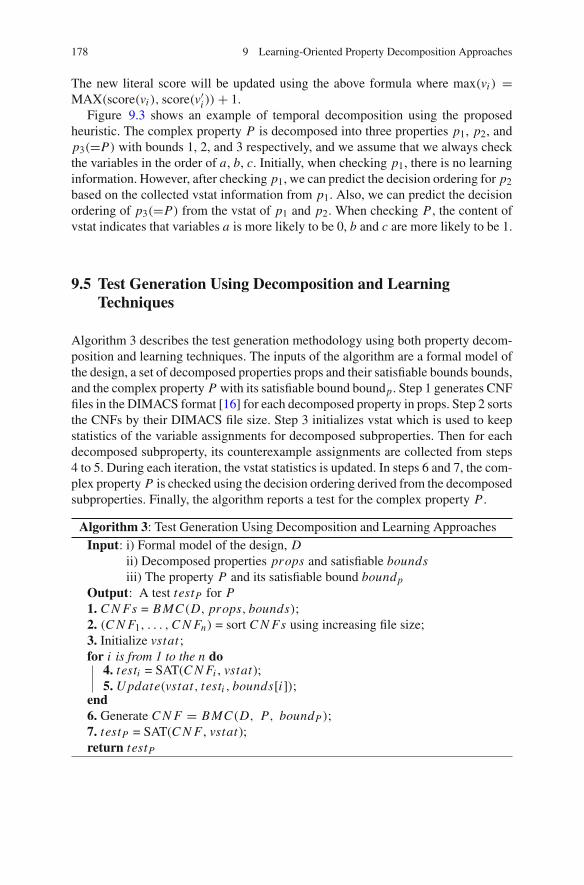
i )) + 1.Figure 9.3 shows an example of temporal decomposition using the proposed
heuristic. The complex property P is decomposed into three properties p1, p2, andp3(=P) with bounds 1, 2, and 3 respectively, and we assume that we always checkthe variables in the order of a, b, c. Initially, when checking p1, there is no learninginformation. However, after checking p1, we can predict the decision ordering for p2based on the collected vstat information from p1. Also, we can predict the decisionordering of p3(=P) from the vstat of p1 and p2. When checking P , the content ofvstat indicates that variables a is more likely to be 0, b and c are more likely to be 1.
9.5 Test Generation Using Decomposition and LearningTechniques
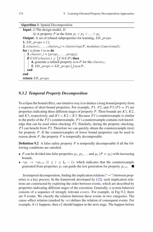
Algorithm 3 describes the test generation methodology using both property decom-position and learning techniques. The inputs of the algorithm are a formal model ofthe design, a set of decomposed properties props and their satisfiable bounds bounds,and the complex property P with its satisfiable bound boundp . Step 1 generates CNFfiles in the DIMACS format [16] for each decomposed property in props. Step 2 sortsthe CNFs by their DIMACS file size. Step 3 initializes vstat which is used to keepstatistics of the variable assignments for decomposed subproperties. Then for eachdecomposed subproperty, its counterexample assignments are collected from steps4 to 5. During each iteration, the vstat statistics is updated. In steps 6 and 7, the com-plex property P is checked using the decision ordering derived from the decomposedsubproperties. Finally, the algorithm reports a test for the complex property P .
Algorithm 3: Test Generation Using Decomposition and Learning ApproachesInput: i) Formal model of the design, D
ii) Decomposed properties props and satisfiable boundsiii) The property P and its satisfiable bound boundp
Output: A test testP for P1. C N Fs = B MC(D, props, bounds);2. (C N F1, . . . , C N Fn) = sort C N Fs using increasing file size;3. Initialize vstat ;for i is from 1 to the n do
4. testi = SAT(C N Fi , vstat);5. U pdate(vstat, testi , bounds[i]);
end6. Generate C N F = B MC(D, P, boundP );7. testP = SAT(C N F , vstat);return testP
9.6 An Illustrative Example 179
9.6 An Illustrative Example
This section presents an example of how to apply decomposition methods onthe graph model of an MIPS processor [7] (described in Sect. 2.2.1). It consistsof five pipeline stages: fetch, decode, execute, memory, and write back. It hasfour pipeline paths in the execute stage: ALU for integer ALU operation, FADDfor floating-point addition operation, MUL for multiply operation, and DIV fordivide operation. Assume that we want to check a complex scenario that the unitsMU L5 and F ADD3 will be active at the same time. We generate the propertyP = ∼F(MU L5.active = 1 & F ADD3.active = 1) which is a negation of thedesired behavior. The remainder of this section describes how to generate a test usingspatial and temporal decomposition methods respectively.
9.6.1 Spatial Decomposition
In the MIPS design, each functional unit has a delay of one clock cycle. To triggerthe functional unit MU L5, we need at least seven clock cycles (there are sevenunits along the path Fetch → Decode → · · · → MUL5). Similarly, to trigger thefunctional unit F ADD3, we need at least five clock cycles, plus one clock cyclefor initialization, we need a total of eight clock cycles for triggering this interaction.Thus the bound of this property is eight. According to Eq. ( 9.2) and Algorithm 1,property P can be spatially decomposed into two subproperties as follows, assumingthe COI of P1 and P2 are both smaller than half of COI of P .
When checking P1 and P2 individually, we can get the following two counterex-amples.
Counterexamples for P1 and P2Cycles P1’s Inst. P2’s Inst.1 NOP NOP2 MUL R2, R2, R0 NOP3 NOP NOP4 NOP FADD R1, R1, R0
However, according to Algorithm 3, the test generation for P2 is under the guid-ance of P1’s result. Thus, the counterexample of P2 guided by P1 contains P1’s
partial behavior (see clock cycle 2 below). So the score of literals which have repet-itive occurrences is enhanced.
Counterexample for P2 guided by P1Cycles P2’s Inst. after learning1 NOP2 MUL R2, R2, R03 NOP4 FADD R1, R1, R0
The statistics saved in vstat indicates an assignment which has a large overlap ofthe assignments with the counterexample that can activate property P . Thus it canbe used as the decision ordering learning to guide the property checking of P .
9.6.2 Temporal Decomposition
Temporal decomposition requires figuring out event relation first. Since we wantto check property ∼F(MU L5.active = 1 & F ADD3.active = 1), the targetevent is MU L5.active = 1 & F ADD3.active = 1. Figure 9.4 shows the eventimplications. There are seven events in this graph, and e7 is the target event.
Assuming e1 is the initial event, from e1 to e7, there is only one path e1 → e2 →e4 → e6 → e7. Along this path there is a branch node e2. According to Algorithm2, we need to check two events e1 and e4 using the following properties. By usingour learning technique, during the test generation, P_e4 can benefit from P_e1, andP can benefit from P_e4.
Fig. 9.5 Test generation results for MIPS processor
9.7 Case Studies
This section presents two case studies: a MIPS architecture [17] (described inSect. 2.2.1) and a stock exchange system (described in Sect. 2.4.4). A tool [12] isdeveloped, which takes a graph model of the design as an input for property decom-position. Based on the analysis of graph model, the process of bound determinationand property decomposition can be automated in this tool. In the experiments, thecost of property decomposition was not considered since it is small (less than 0.01s).For test generation, NuSMV [18] was used to derive the CNF clauses (in DIMACSformat) and integrated the proposed methods in the SAT solver zChaff [16]. Theexperimental results were obtained on a Linux PC using 2.0GHz Core 2 Duo CPUwith 1 GB RAM.
9.7.1 A MIPS Processor
This section presents the experimental results using the same design illustrated inSect. 9.6. For the MIPS design, we are focusing on the test generation of interactionfaults. The properties were generated in the form of ¬F(p1&p2& . . . &pn) whichindicate whether n pipelined components pi (1 ≤ i ≤ n) can be activated at thesame time. For example, the property ∼F(MU L6.active = 1&F ADD3.active =1&DI V .active = 1) asserts that there is no instruction sequence which can activatethe components MU L6, F ADD3, and DI V at the same time.
A set of 20 properties were generated based on various interaction faults. Sinceit is hard to figure out the temporal relation between events, six properties of themcannot be handled by temporal decomposition. Table 9.1 shows the test generationresults using the spatial decomposition approach for such properties. The first col-umn indicates the selected properties. The second column gives the test generationtime using zChaff. The third and fourth columns present the number of subpropertyclusters and the number of refined subproperties for deriving learnings. The last twocolumns show test generation time using the spatial decomposition method (includ-ing the overhead of subproperty checking) and its improvement over the methodusing zChaff. Compared with the method without any learnings (column 2), the spa-tial decomposition-based learning method can drastically reduce the test generationtime.
For the remaining 14 properties, both spatial and temporal decomposition areapplied individually. Figure 9.5 illustrates the performance improvement over themethod using zChaff. It shows that the temporal method can drastically reduce testgeneration time (2–4 times). Although spatial decomposition outperforms temporaldecomposition in this case study, comparing with the method using zChaff, temporaldecomposition can still have significant improvement (2.5 times).
9.7.2 A Stock Exchange System
The online stock exchange system (OSES) is a software which mainly deals withstock order transactions. The specification of OSES is described by a UML activitydiagram which contains 27 activities and 29 transitions. We extract the formal modelfrom the UML specification and transform it into a NuSMV description. We generate18 complex properties to check various stock transactions. Each transaction is asequence of activities (events). The test generation for a transaction using only onecomplex property is time-consuming. So we temporally decomposed the transactioninto several stages which specify the branch activities along the path, and for eachstage we create a subproperty.
9.7 Case Studies 183
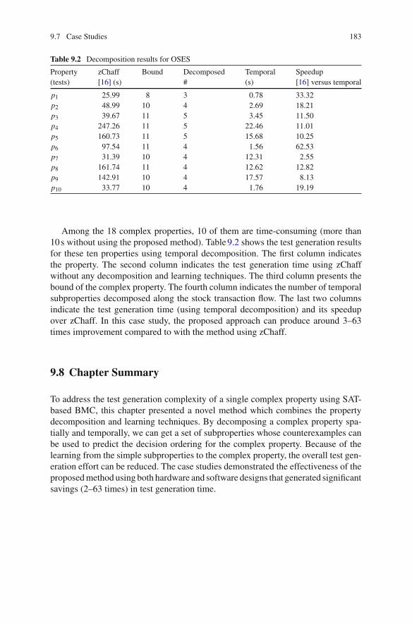
Table 9.2 Decomposition results for OSES
Property zChaff Bound Decomposed Temporal Speedup(tests) [16] (s) # (s) [16] versus temporal
Among the 18 complex properties, 10 of them are time-consuming (more than10 s without using the proposed method). Table 9.2 shows the test generation resultsfor these ten properties using temporal decomposition. The first column indicatesthe property. The second column indicates the test generation time using zChaffwithout any decomposition and learning techniques. The third column presents thebound of the complex property. The fourth column indicates the number of temporalsubproperties decomposed along the stock transaction flow. The last two columnsindicate the test generation time (using temporal decomposition) and its speedupover zChaff. In this case study, the proposed approach can produce around 3–63times improvement compared to with the method using zChaff.
9.8 Chapter Summary
To address the test generation complexity of a single complex property using SAT-based BMC, this chapter presented a novel method which combines the propertydecomposition and learning techniques. By decomposing a complex property spa-tially and temporally, we can get a set of subproperties whose counterexamples canbe used to predict the decision ordering for the complex property. Because of thelearning from the simple subproperties to the complex property, the overall test gen-eration effort can be reduced. The case studies demonstrated the effectiveness of theproposed method using both hardware and software designs that generated significantsavings (2–63 times) in test generation time.
1. Biere A, Cimatti A, Clarke EM, Strichman O, Zhu Y (2003) Bounded model checking. AdvComput 58:117–148
2. Case ML, Mony H, Baumgartner J, Kanzelman R (2009) Enhanced verification by temporaldecomposition. In: Proceedings of international conference on formal methods in computer-aided design (FMCAD), pp 17–24
3. Lin H, Jiang J, Lee R (2008) To SAT or not to SAT: Ashenhurst decomposition in a large scale.In: Proceedings of international conference on computer-aided design (ICCAD), pp 32–37
4. Koo H, Mishra P (2009) Functional test generation using design and property decompositiontechniques. ACM Trans Embed Comput Syst 8(4):32:1–32:33
5. Strichman O (2001) Pruning techniques for the SAT-based bounded model checking problem.In: Proceedings of correct hardware design and verification methods (CHARME), pp 58–70
6. Jin H, Somenzi F (2004) An incremental algorithm to check satisfiability for bounded modelchecking. In: Proceedings of BMC, pp 51–65
7. Chen M, Mishra P (2010) Functional test generation using efficient property clustering andlearning techniques. IEEE Trans Comput Aided Des Integr Circuits Syst 29(3):396–404
8. Marques-Silva JP, Sakallah KA (1999) The impact of branching heuristics in propositionalsatisfiability. In: Proceedings of the 9th portuguese conference on artificial intelligence, pp62–74
9. Shtrichman O (2000) Tuning SAT checkers for bounded model checking. In: Proceedings ofthe The international conference on computer aided verification (CAV), pp 480–494
10. Wang C, Jin H, Hachtel GD, Somenzi F (2004) Refining the SAT decision ordering for boundedmodel checking. In: Proceedings of design automation conference (DAC), pp 535–538
11. Chen M, Qin X, Mishra P (2010) Efficient decision ordering techniques for SAT-based testgeneration. In: Proceedings of design, automation and test in Europe (DATE), pp 490–495
12. Chen M, Mishra P (2011) Decision ordering based property decomposition for functional testgeneration. In: Proceedings of design, automation and test in Europe (DATE), pp 167–172
13. Clarke E, Grumberg O, Peled D (1999) Model checking. MIT Press, Cambridge14. Dijkstra EW (1959) A note on two problems in connexion with graphs. Numerische mathematik
1:269–27115. Moskewicz M, Madigan C, Zhao Y, Zhang L, Malik S (2001) Chaff: engineering an efficient
SAT solver. In: Proceedings of design automation conference (DAC), pp 530–53516. zChaff (2004) http://www.princeton.edu/~chaff/zchaff.html17. Hennessy J, Patterson D (2003) Computer architecture: a quantitative approach. Morgan Kauf-
mann Publishers, San Francisco18. NuSMV. http://nusmv.irst.itc.it