Page 1
T H E U N I V E R S I T Y O F T U L S A
THE GRADUATE SCHOOL
OIL-WATER SEPARATION IN LIQUID-LIQUID HYDROCYCLONES (LLHC)
EXPERIMENT AND MODELING
by
Carlos Hernán Gómez
A Thesis Submitted in Partial Fulfillment of
the Requirements for the Degree of Master of Science
in the Discipline of Petroleum Engineering
The Graduate School
The University of Tulsa
2001
Page 2
ii
T H E U N I V E R S I T Y O F T U L S A
THE GRADUATE SCHOOL
OIL-WATER SEPARATION IN LIQUID-LIQUID HYDROCYCLONES (LLHC)
EXPERIMENT AND MODELING
by
Carlos Hernán Gómez
A THESIS
APPROVED FOR THE DISCIPLINE OF
PETROLEUM ENGINEERING
By Thesis Committee
_____________________________________, Co-Chairperson Dr. Ovadia Shoham
_____________________________________, Co-Chairperson Dr. Ram S. Mohan
_____________________________________ Dr. Mauricio Prado
_____________________________________ Dr. Grant Young
Page 3
iii
ABSTRACT
Gómez, Carlos Hernan (Master of Science in Petroleum Engineering)
Oil-Water Separation in Liquid-Liquid Hydrocyclones (LLHC) Experiment and
Modeling
(102 pp. Chapter VI)
Directed by Professor Ovadia Shoham and Professor Ram S. Mohan
(427 words)
The liquid-liquid hydrocyclone (LLHC) has been widely used by the Petroleum
Industry for the past several decades. A large quantity of information on the LLHC
available in the literature includes experimental data, computational fluid dynamic
simulations and field applications. The design of LLHCs has been based in the past
mainly on empirical experience. However, no simple and overall design mechanistic
model has been developed to date for the LLHC. Also, there exists the need for accurate
experimental data including the measurements of the droplet size distributions at the inlet
and underflow streams.
A new facility for testing LLHCs was designed, constructed and installed in an
existing three-phase flow loop. The test section is fully instrumented to measure the
important flow and separation variables. A total of 124 experimental runs were
conducted, for each of which the acquired data include flow rates, oil concentrations,
droplet size distributions, pressures and temperature. Utilization of static mixers enabled
the generation of a wide range of droplet size distributions at the LLHC inlet. A droplet
Page 4
iv
size distribution analyzer was utilized to obtain the droplet size distribution from the
samples.
The data reveal that LLHCs can be used up to 10% oil concentrations at the inlet,
maintaining high separation efficiency. However, the performance of the LLHC is best
for very low oil concentrations at the inlet, below 1%. For low concentrations, no
emulsification of the mixture occurs in the LLHC. However, high inlet concentrations,
up to 10%, promote emulsification posing a separation problem in the overflow stream.
An existing LLHC mechanistic model is modified and refined. The main
modifications carried out are improved correlation for the swirl intensity that affects the
axial and tangential velocity distributions, the flow reversal radius and the inlet factor.
The required inputs for the model are: LLHC geometry, fluid properties, inlet droplet size
distribution and operational conditions. The model is capable of predicting the LLHC
hydrodynamic flow field, namely, the swirl intensity and the axial, tangential and radial
velocity distributions of the continuous-phase. The separation efficiency and migration
probability are determined based on droplet trajectory analysis. The flow capacity,
namely, the inlet-to-underflow pressure drop, is predicted utilizing an energy balance
analysis.
The LLHC mechanistic model was tested against the present study data and
additional data from the literature, especially from Colman and Thew (1980). Very good
agreement is observed between the model predictions and the experimental data with
respect to the swirl intensity, axial and tangential velocity distributions, migration
probability and global separation efficiency. The developed LLHC model can be used
for the design of field applications for the industry.
Page 5
v
ACKNOWLEDGEMENTS
I want to thank the following persons for their support and guidance during my study:
Dr. Ovadia Shoham for assisting and advising this study.
Dr. Ram Mohan, my co-advisor for his collaboration.
Dr. Mauricio Prado and Dr. Grant Young for participating on my thesis committee.
My Family; Sandra Milena, Juan Sebastian and Carlos Andres.
Mr. Luis Tineo and My sister Mayda Johana.
TUSTP Group.
The University of Tulsa, Petroleum Engineering Staff.
Page 6
vi
TABLE OF CONTENTS
TITLE PAGE i
APPROVAL PAGE ii
ABSTRACT iii
ACKNOWLEDGMENTS v
TABLE OF CONTENTS vi
LIST OF FIGURES viii
LIST OF TABLES x
CHAPTER I
INTRODUCTION 1
CHAPTER II
LITERATURE REVIEW 8
2.1 Experimental Studies 10
2.2 Modeling and CFD Simulations 13
CHAPTER III
EXPERIMENTAL PROGRAM 19
3.1 Experimental Facility Description 19
3.1.1 Storage and Metering Section 20
3.1.2 Test Section 21
3.1.3 Downstream Oil-Water Separation Section 24
3.1.4 Data Acquisition System 24
3.2 Working Fluids 25
3.3 Definition of Separation Parameters 25
3.3.1 Split Ratio 25
3.3.2 Oil Separation Efficiency 27
3.4 Experimental Results 27
3.4.1 Effect of Pressure Drop and Flow Rate 28
3.4.2 Effect of Underflow Pressure 28
3.4.3 Effect of Overflow Diameter 29
Page 7
vii
3.4.4 Effect of Inlet Oil Concentration 31
3.4.5 Effect of Oil Droplet Distribution 31
CHAPTER IV
LLHC MECHANISTIC MODEL 34
4.1 Swirl Intensity 34
4.2 Velocity Field 36
4.3 Droplet Trajectories 40
4.4 Separation Efficiency 43
4.5 Pressure Drop 46
4.6 LLHC Mechanistic Model Code 48
CHAPTER V
RESULTS AND DISCUSSION 50
5.1 Global Separation Efficiency 50
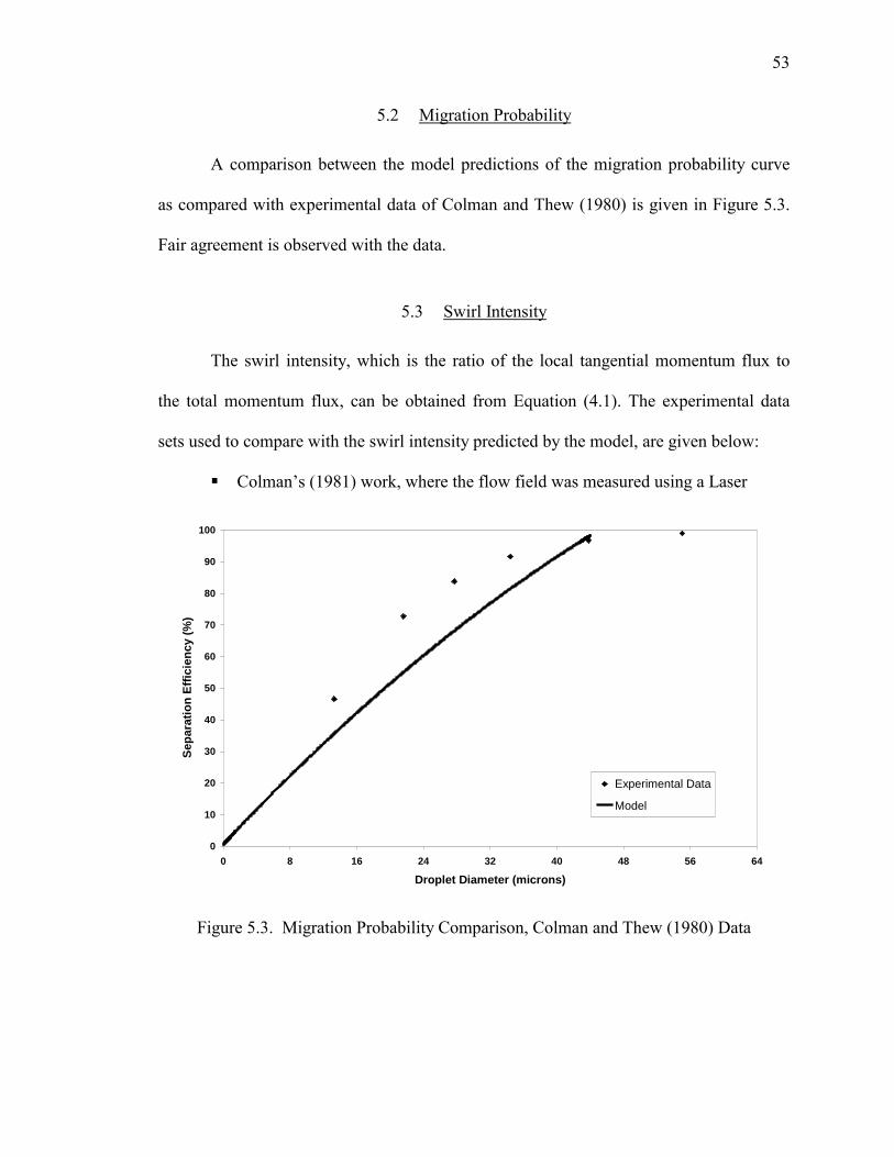
5.2 Migration Probability 53
5.3 Swirl Intensity 53
5.4 Velocity Profile 57
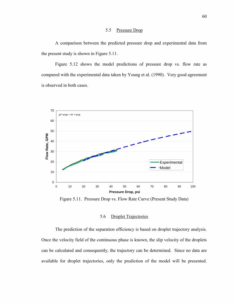
5.5 Pressure Drop 60
5.6 Droplet Trajectories 60
5.7 Droplet Size Distribution 63
CHAPTER VI
SUMMARY, CONCLUSIONS AND RECOMMENDATIONS 65
6.1 Summary and Conclusions 65
6.2 Recommendations 67
NOMENCLATURE 69
REFERENCES 72
APPENDICES 79
Page 8
viii
LIST OF FIGURES
Figure 1.1 LLHC Hydrodynamic Flow Behavior 3
Figure 1.2 Colman and Thews Hydrocyclone Geometry 5
Figure 1.3 LLHC Inlet Design 6
Figure 2.1 Tangential Velocity Diagram 15
Figure 3.1 Schematic of Experimental LLHC Flow Loop 19
Figure 3.2 Schematic of LLHC Test Section 22
Figure 3.3 Photograph of LLHC Test Section 22
Figure 3.4 Schematic of Isokinetic Sampling Probe 23
Figure 3.5 Effect of Pressure Drop or Flow Rate on Efficiency 28
Figure 3.6 Effect of Underflow Pressure on Efficiency 29
Figure 3.7 Effect of Overflow Diameter on Efficiency 30
Figure 3.8 Effect of Oil Concentration on Efficiency 31
Figure 3.9 Effect of Droplet Size Distribution on Efficiency 32
Figure 3.10 Typical Measured Droplet Size Distributions 32
Figure 3.11 Typical Output of Droplet Size Analyzer (Test 101) 33
Figure 4.1 Rankine Vortex Tangential Velocity Profile 37
Figure 4.2 Axial Velocity Diagram 38
Figure 4.3 Schematic of Droplet Trajectory Model 41
Figure 4.4 Schematic of Droplet Trajectory and Separation Efficiency 44
Figure 4.5 Migration Probability Curve 45
Figure 4.6 LLHC Mechanistic Model Code 49
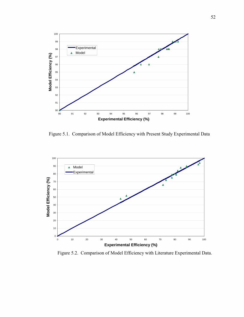
Figure 5.1 Comparison of Model Efficiency with Present Study Experimental Data 52
Figure 5.2 Comparison of Model Efficiency with Literature Experimental Data 52
Figure 5.3 Migration Probability Comparison, Colman and Thew (1980) Data 53
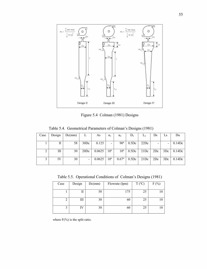
Figure 5.4 Colman (1981) Designs 55
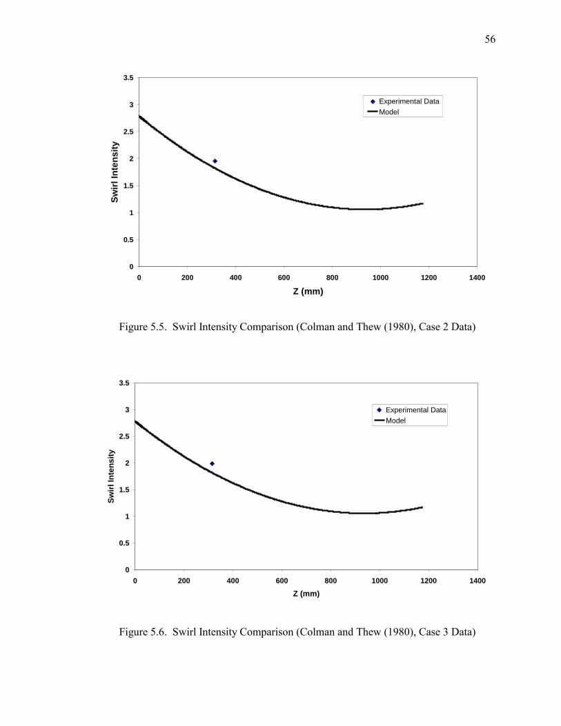
Figure 5.5 Swirl Intensity Comparison (Colman and Thew (1980) Case 2 Data) 56
Figure 5.6 Swirl Intensity Comparison (Colman and Thew (1980) Case 3 Data) 56
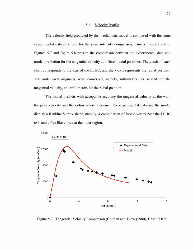
Figure 5.7 Tangential Velocity Comparison (Colman and Thew (1980), Case 2
Page 9
ix
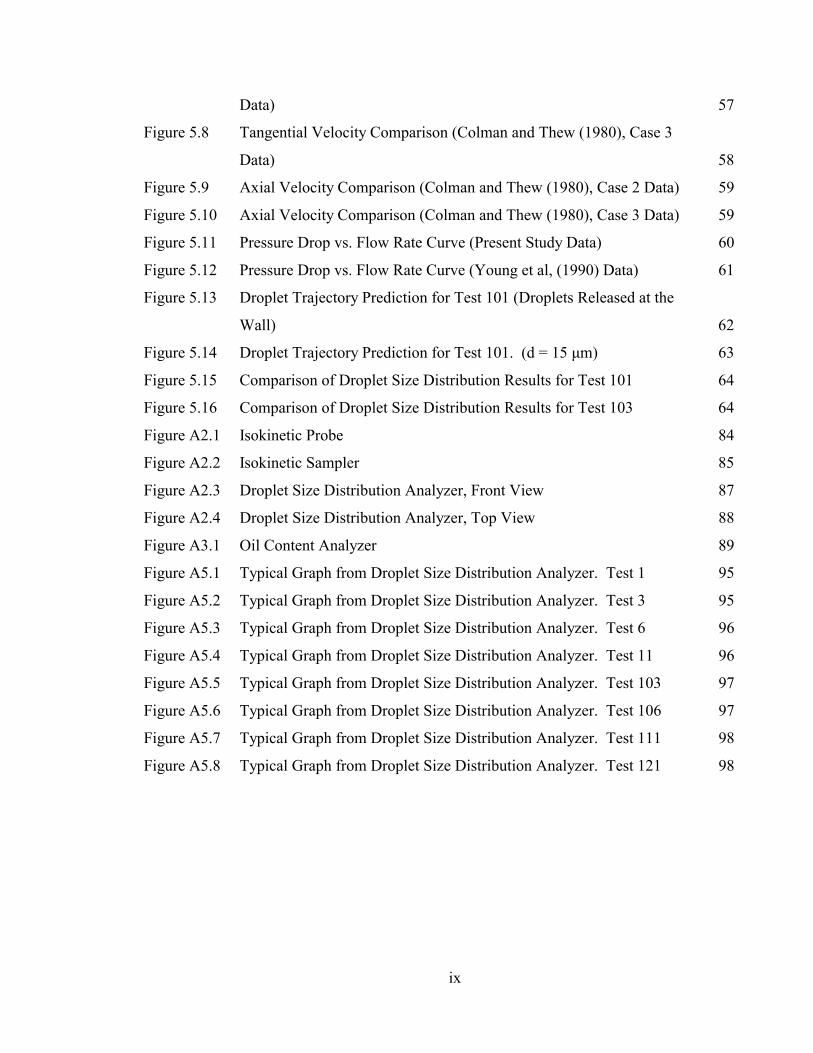
Data) 57
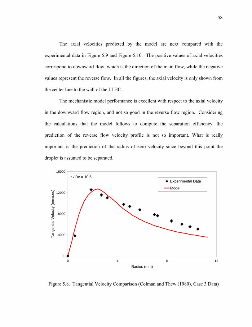
Figure 5.8 Tangential Velocity Comparison (Colman and Thew (1980), Case 3
Data) 58
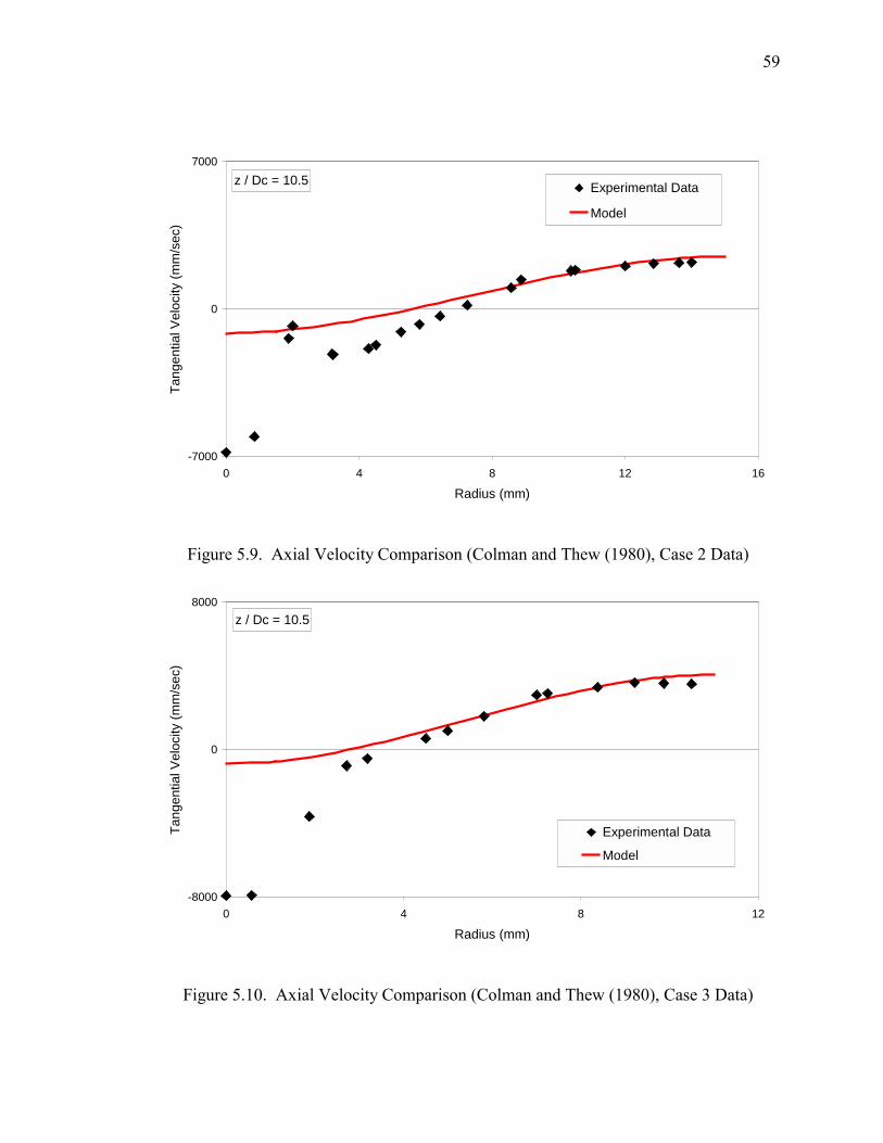
Figure 5.9 Axial Velocity Comparison (Colman and Thew (1980), Case 2 Data) 59
Figure 5.10 Axial Velocity Comparison (Colman and Thew (1980), Case 3 Data) 59
Figure 5.11 Pressure Drop vs. Flow Rate Curve (Present Study Data) 60
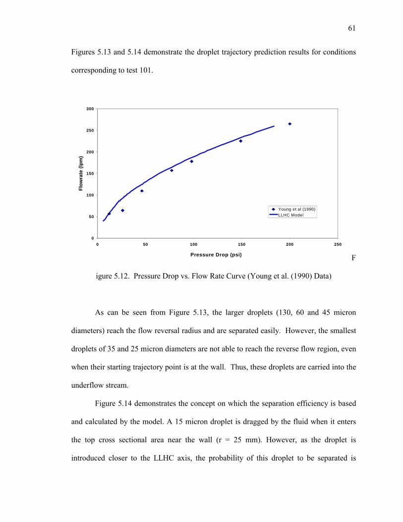
Figure 5.12 Pressure Drop vs. Flow Rate Curve (Young et al, (1990) Data) 61
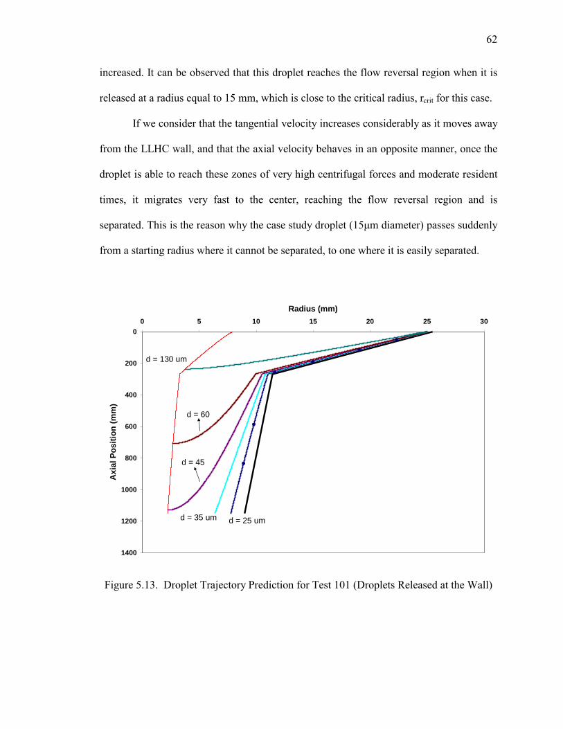
Figure 5.13 Droplet Trajectory Prediction for Test 101 (Droplets Released at the
Wall) 62
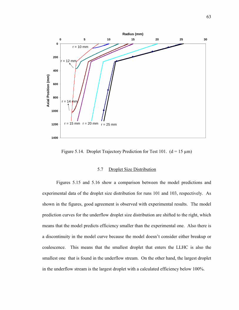
Figure 5.14 Droplet Trajectory Prediction for Test 101. (d = 15 µm) 63
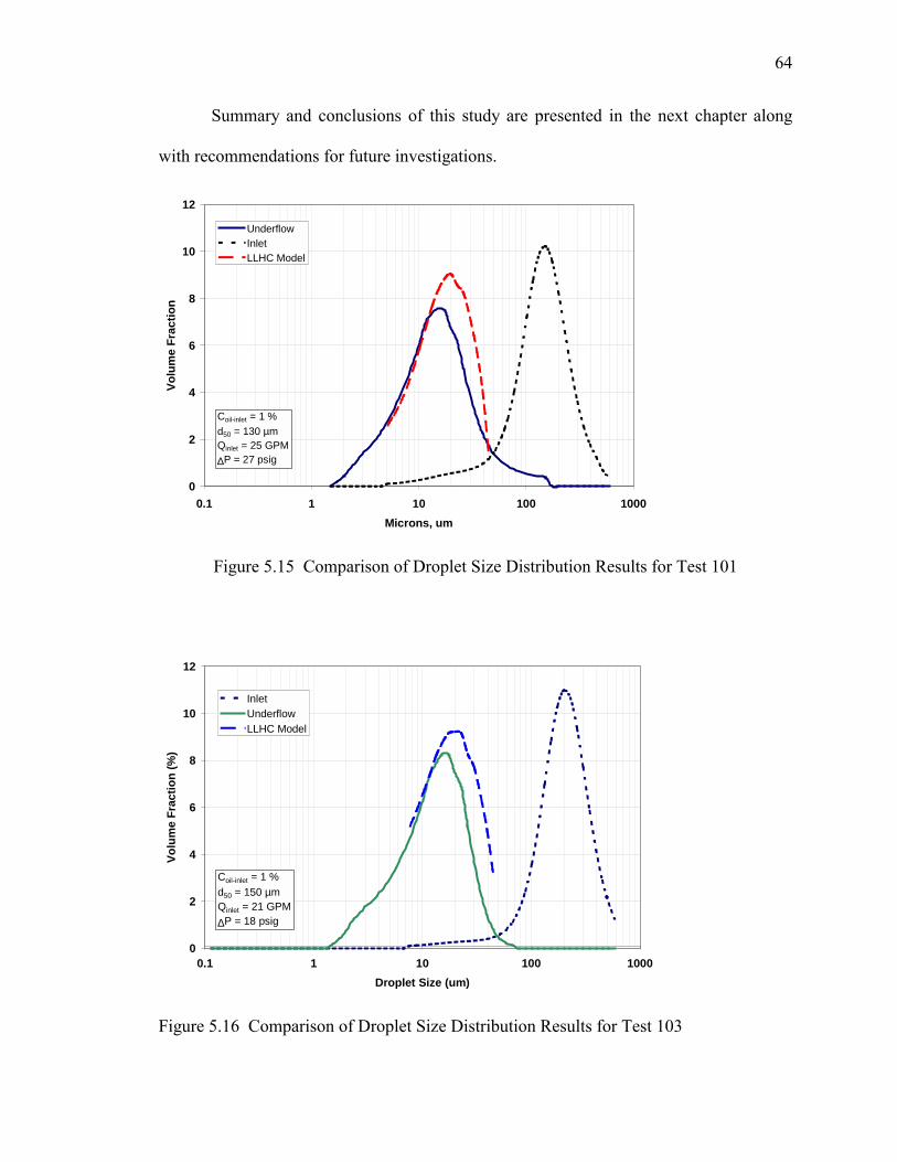
Figure 5.15 Comparison of Droplet Size Distribution Results for Test 101 64
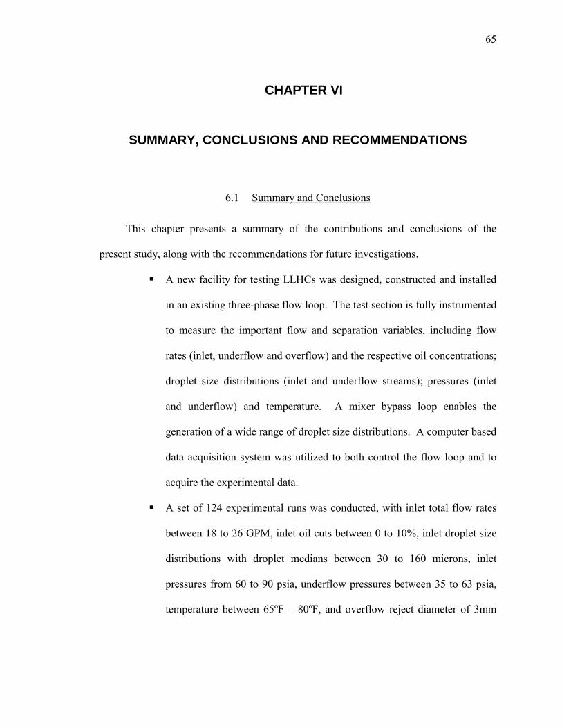
Figure 5.16 Comparison of Droplet Size Distribution Results for Test 103 64
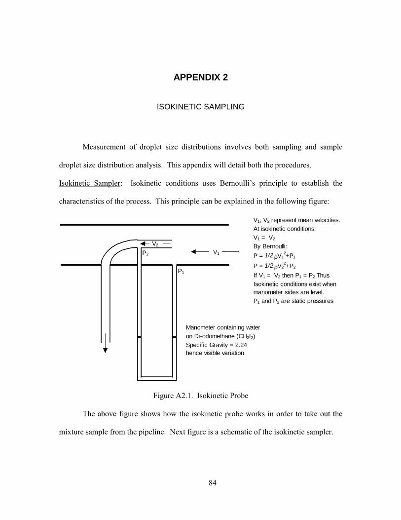
Figure A2.1 Isokinetic Probe 84
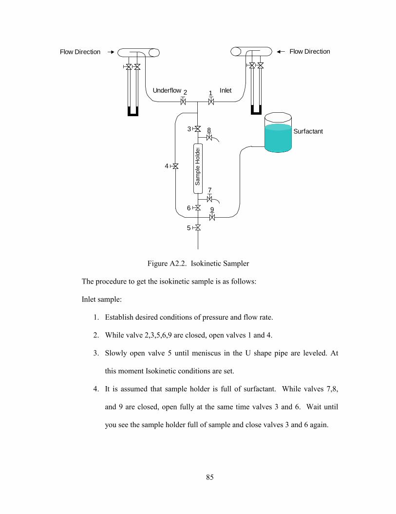
Figure A2.2 Isokinetic Sampler 85
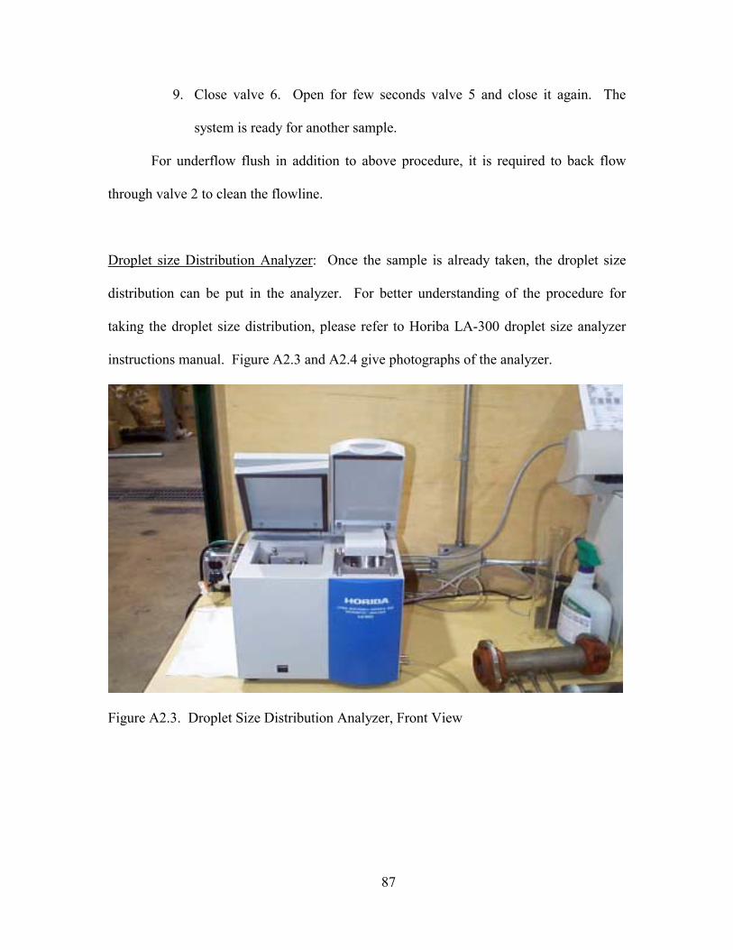
Figure A2.3 Droplet Size Distribution Analyzer, Front View 87
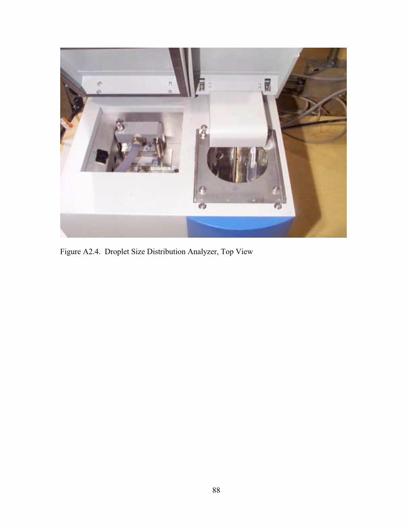
Figure A2.4 Droplet Size Distribution Analyzer, Top View 88
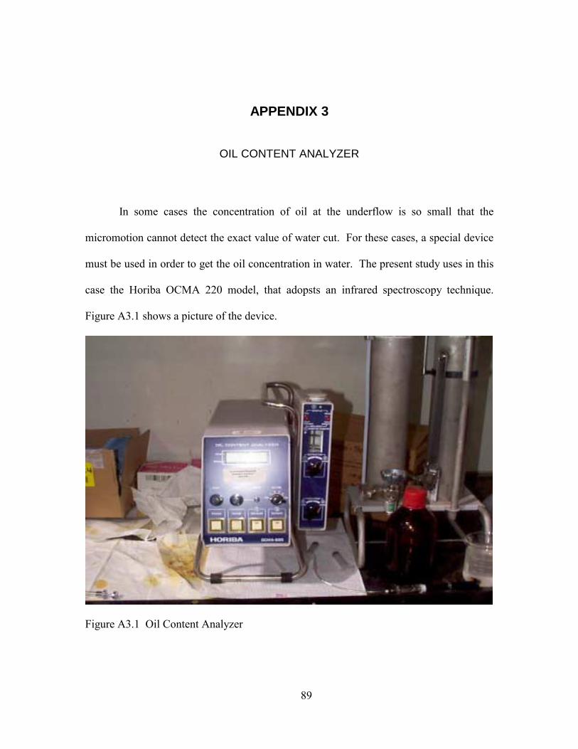
Figure A3.1 Oil Content Analyzer 89
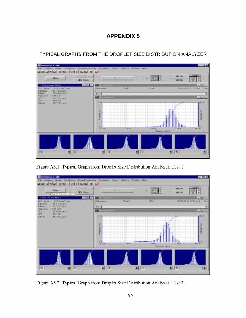
Figure A5.1 Typical Graph from Droplet Size Distribution Analyzer. Test 1 95
Figure A5.2 Typical Graph from Droplet Size Distribution Analyzer. Test 3 95
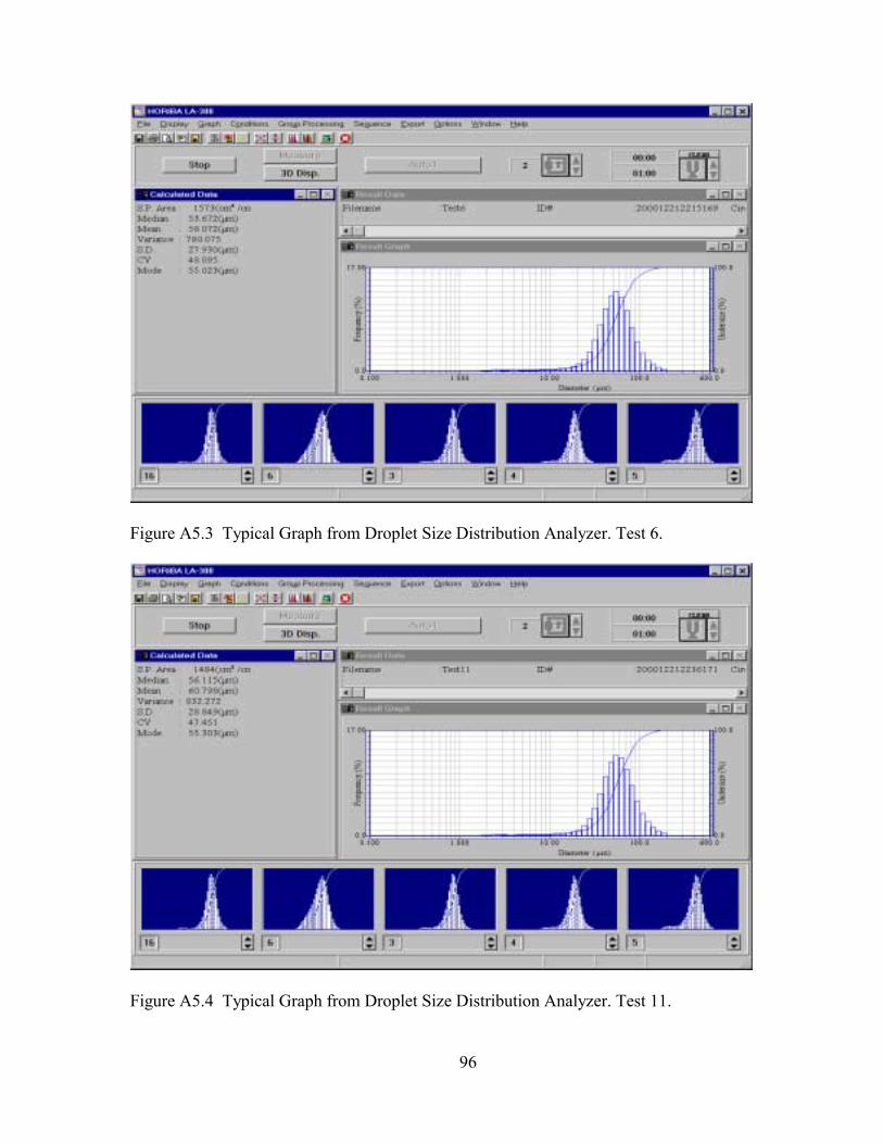
Figure A5.3 Typical Graph from Droplet Size Distribution Analyzer. Test 6 96
Figure A5.4 Typical Graph from Droplet Size Distribution Analyzer. Test 11 96
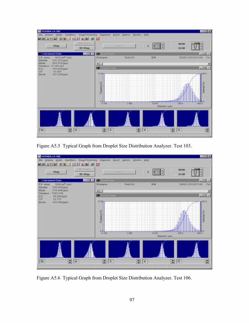
Figure A5.5 Typical Graph from Droplet Size Distribution Analyzer. Test 103 97
Figure A5.6 Typical Graph from Droplet Size Distribution Analyzer. Test 106 97
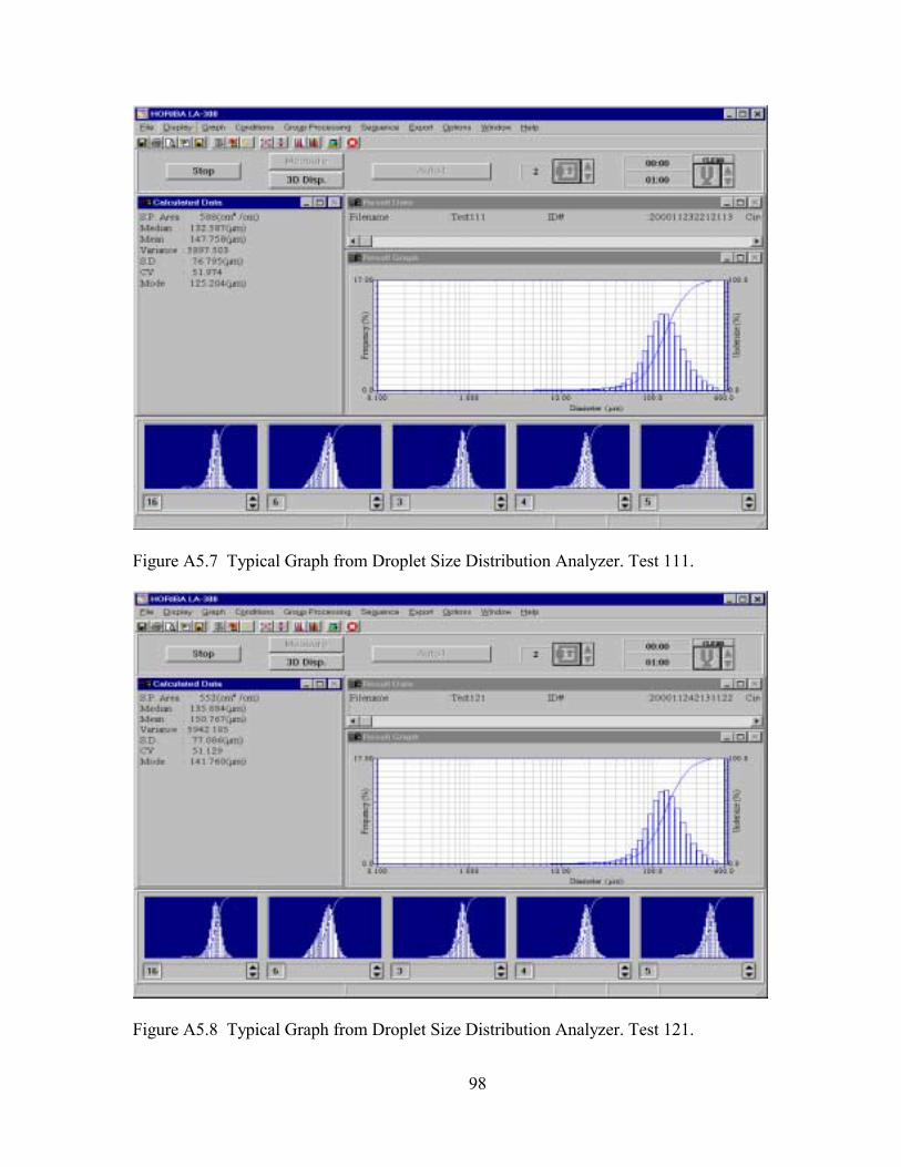
Figure A5.7 Typical Graph from Droplet Size Distribution Analyzer. Test 111 98
Figure A5.8 Typical Graph from Droplet Size Distribution Analyzer. Test 121 98
Page 10
x
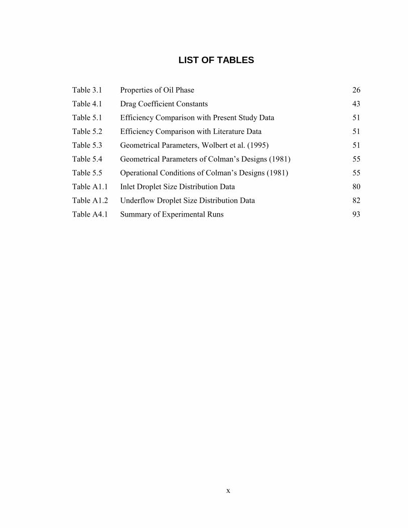
LIST OF TABLES
Table 3.1 Properties of Oil Phase 26
Table 4.1 Drag Coefficient Constants 43
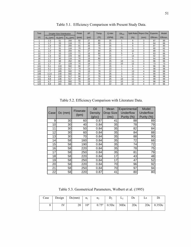
Table 5.1 Efficiency Comparison with Present Study Data 51
Table 5.2 Efficiency Comparison with Literature Data 51
Table 5.3 Geometrical Parameters, Wolbert et al. (1995) 51
Table 5.4 Geometrical Parameters of Colmans Designs (1981) 55
Table 5.5 Operational Conditions of Colmans Designs (1981) 55
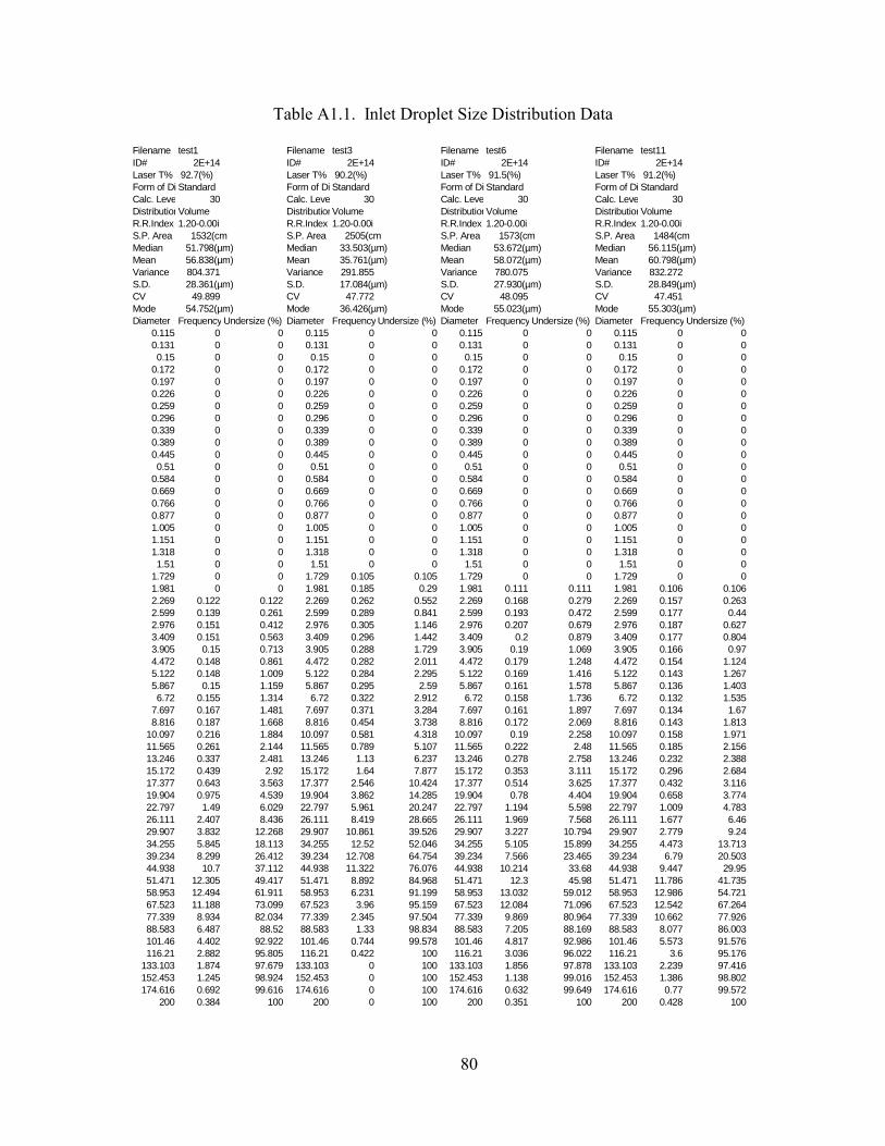
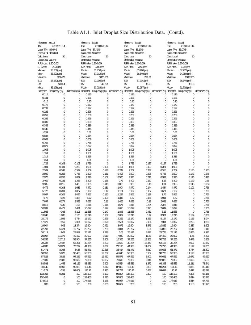
Table A1.1 Inlet Droplet Size Distribution Data 80
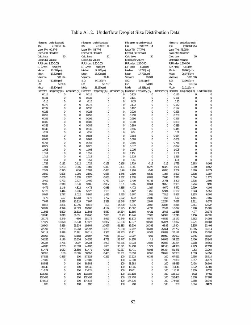
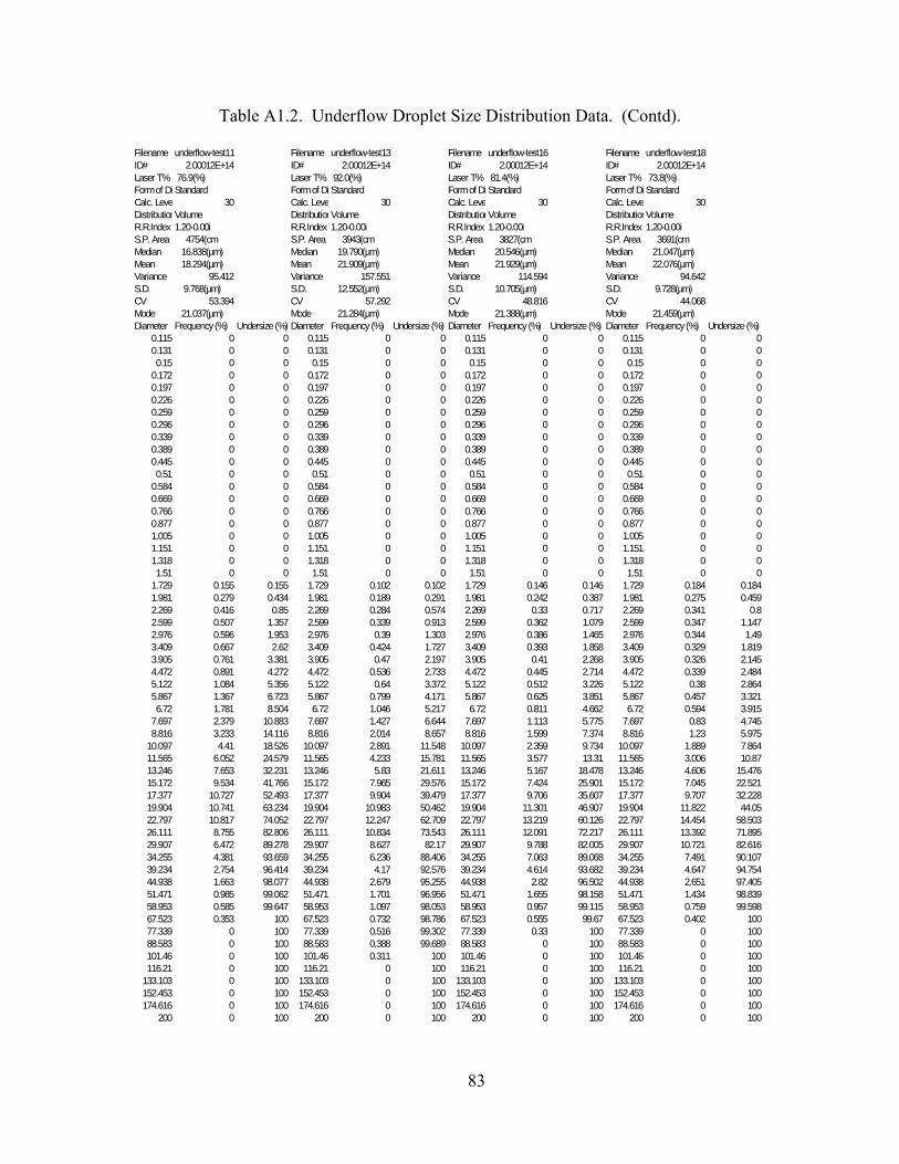
Table A1.2 Underflow Droplet Size Distribution Data 82
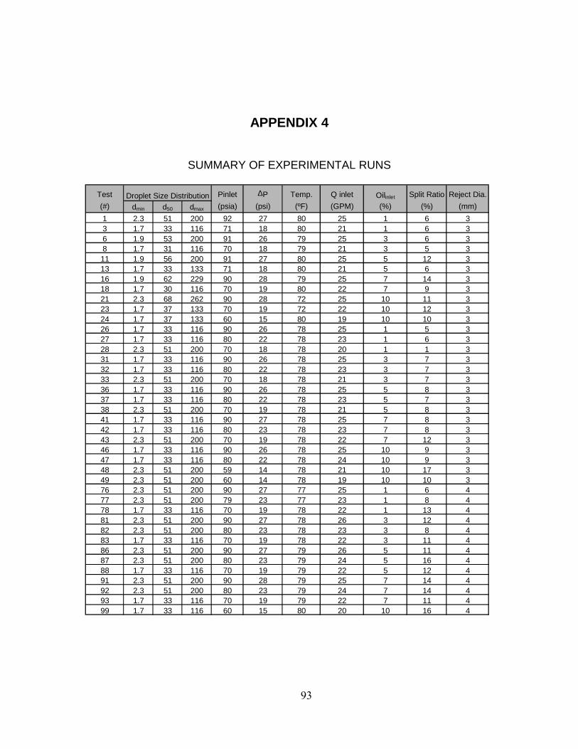
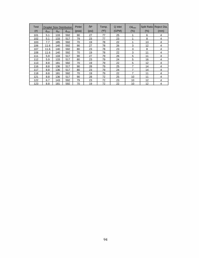
Table A4.1 Summary of Experimental Runs 93
Page 11
1
CHAPTER I
INTRODUCTION
1.1 Motivation and Objective
The petroleum industry has traditionally relied on conventional gravity based
vessels, that are bulky, heavy and expensive, to separate multiphase flow. The growth of
the offshore oil industry, where platform costs to accommodate these separation facilities
are critical, has provided the incentive for the development of compact separation
technology. Hydrocyclones have emerged as an economical and effective alternative for
produced water deoiling and other applications. The hydrocyclone is inexpensive, simple
in design with no moving parts, easy to install and operate, and has low maintenance cost.
Hydrocyclones have been used in the past to separate solid-liquid, gas-liquid and
liquid-liquid mixtures. For the liquid-liquid case, both dewatering and deoiling have been
used in the oil industry. This study focuses only on the latter case, namely, using the
liquid-liquid hydrocyclones (LLHC) to remove dispersed oil from a water continuous
stream.
Oil is produced with significant amount of water and gas. Typically, a set of
conventional gravity based vessels are used to separate most of the multiphase mixture.
The small amount of oil remaining in the water stream, after the primary separation, has
to be reduced to a legally allowable minimum level for offshore disposal. LLHCs have
been used successfully to achieve this environmental regulation.
Page 12
2
There is a large quantity of literature available on the LLHC, including
experimental data sets and computational fluid dynamic simulations. However, there is
still a need for more comprehensive data sets, including measurements of the underflow
droplet size distribution. Additionally, there is a need for a simple and overall
mechanistic model for the LLHC.
The objective of the present study is to acquire new experimental data for the
LLHC, including appropriate sampling procedure and detailed measurements of the
droplet size distributions in the inlet and underflow streams. The new data will be used
to test an existing mechanistic model for the LLHC. Modification and refinement of the
mechanistic model will be carried out, as necessary.
The developed mechanistic model can be utilized for the design of LLHCs,
providing the flexibility of designing alternative LLHC geometries for the same operating
conditions for optimization purposes. It will also allow detailed analysis and
performance prediction for a given LLHC geometry and operating conditions, including
separation efficiency and flow capacity (pressure drop flow rate relationship).
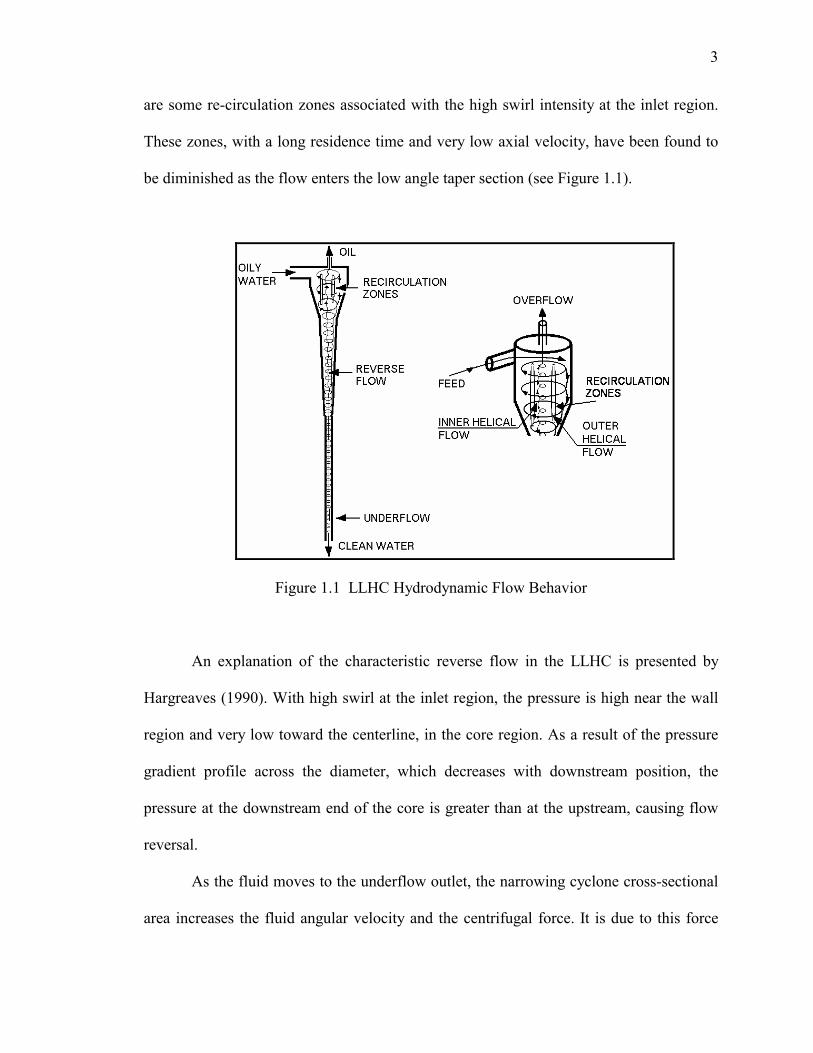
1.2 LLHC Hydrodynamic Flow Behavior
The LLHC, shown in Figure 1.1, utilizes the centrifugal force to separate the
dispersed phase from the continuous fluid. The swirling motion is produced by the
tangential injection of pressurized fluid into the hydrocyclone body. The flow pattern
consists of a spiral within another spiral moving in the same circular direction (Seyda and
Petty, 1991). There is a forced vortex in the region close to the LLHC axis and a free-like
vortex in the outer region. The outer vortex moves downward to the underflow outlet,
while the inner vortex flows in a reverse direction to the overflow outlet. Moreover, there
Page 13
3
are some re-circulation zones associated with the high swirl intensity at the inlet region.
These zones, with a long residence time and very low axial velocity, have been found to
be diminished as the flow enters the low angle taper section (see Figure 1.1).
Figure 1.1 LLHC Hydrodynamic Flow Behavior
An explanation of the characteristic reverse flow in the LLHC is presented by
Hargreaves (1990). With high swirl at the inlet region, the pressure is high near the wall
region and very low toward the centerline, in the core region. As a result of the pressure
gradient profile across the diameter, which decreases with downstream position, the
pressure at the downstream end of the core is greater than at the upstream, causing flow
reversal.
As the fluid moves to the underflow outlet, the narrowing cyclone cross-sectional
area increases the fluid angular velocity and the centrifugal force. It is due to this force
Page 14
4
and the difference in density between the oil and the water, that the oil moves to the
center, where it is caught by the reverse flow and separated, flowing into the overflow
outlet. Instead, if the dispersed phase is the heavier, like solid particles, it will migrate to
the wall and exit through the underflow.
The amount of fluid going through the different outlets differs with heavy and
light dispersion. It means that for these two different separation cases, two different
geometries are needed (Seyda and Petty, 1991). In the deoiling case, usually between 1 to
10 percent of the feed flow rate goes to the overflow.
Another phenomenon that may occur in a hydrocyclone is the formation of a gas
core. As Thew (1986) explained, dissolved gas may come out of solution because of the
pressure reduction in the core region, migrating fast to the LLHC axis, and eventually
emerging through the overflow outlet. A significant amount of gas can be tolerated but
excessive amounts will disturb the vortex. An experimental study on this topic is found in
Smyth and Thew (1996).
1.3 LLHC Geometry
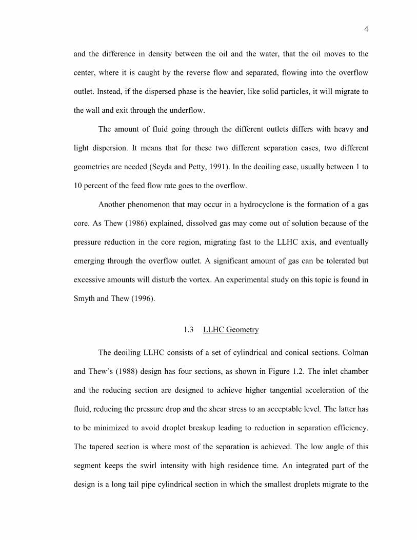
The deoiling LLHC consists of a set of cylindrical and conical sections. Colman
and Thews (1988) design has four sections, as shown in Figure 1.2. The inlet chamber
and the reducing section are designed to achieve higher tangential acceleration of the
fluid, reducing the pressure drop and the shear stress to an acceptable level. The latter has
to be minimized to avoid droplet breakup leading to reduction in separation efficiency.
The tapered section is where most of the separation is achieved. The low angle of this
segment keeps the swirl intensity with high residence time. An integrated part of the
design is a long tail pipe cylindrical section in which the smallest droplets migrate to the
Page 15
5
reversed flow core at the axis and are being separated flowing into the overflow exit. This
configuration gives a very stable small diameter reversed flow core, utilizing a very small
overflow port.
Figure 1.2 Colman and Thews Hydrocyclone Geometry
Young et al. (1990) achieved similar results to Colman-Thews LLHC, in terms of
separation efficiency, with a different hydrocyclone configuration. Three sections were
used instead of four. The reducing section was eliminated and the angle of the tapered
section was changed from 1.5º to 6º. Later, Young et al. (1993) developed a new LLHC
design, which resulted in an improvement in the separation performance. The principal
modification of the enhanced design was a small change in the tail pipe section. A minute
angle conical section was used rather than the cylindrical pipe.
Page 16
6
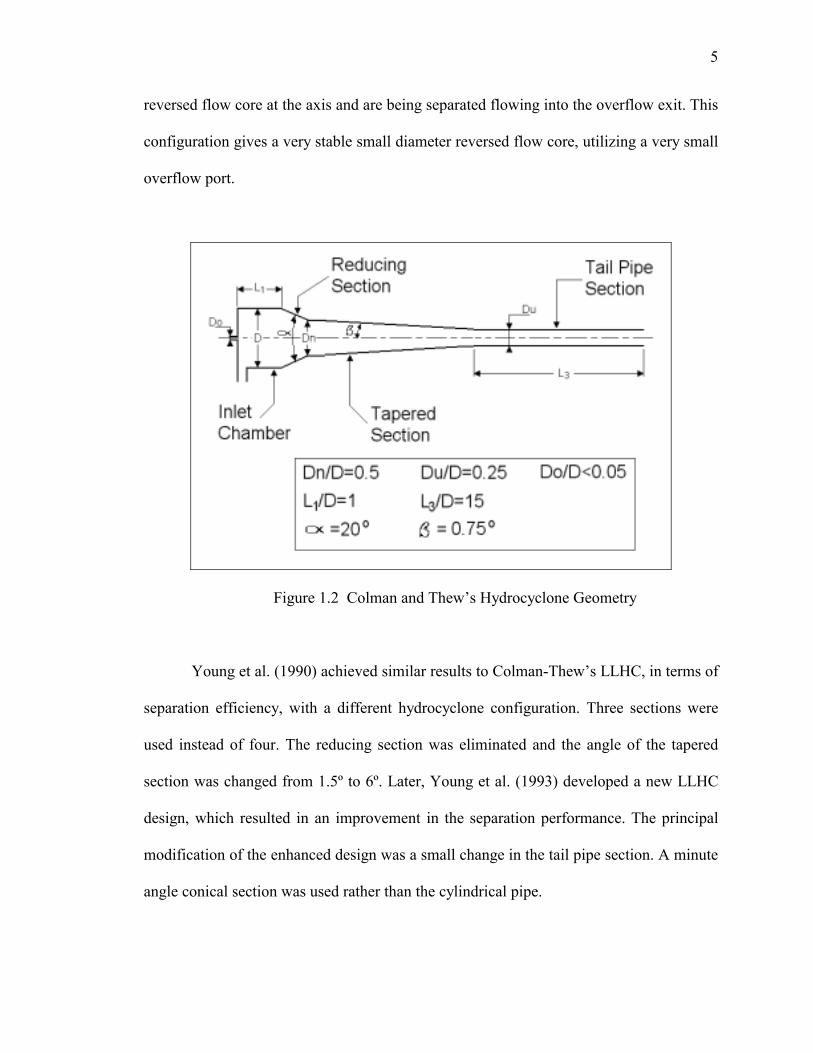
Another important parameter in the LLHC geometry is the inlet configuration, as
shown in Figure 1.3. Rectangular and circular, single and twin inlets have been most
frequently used by different researchers. The main goal is to inject the fluid with higher
tangential velocity, avoiding the rupture of the droplets. The twin inlets have been
considered to maintain better symmetry and for this reason maintain a more stable
reverse core (Colman et al., 1984; Thew et al., 1984). Good results have also been
achieved with the involute single inlet design.
Figure 1.3 LLHC Inlet Design
The last element of the LLHC is the overflow outlet. This is a very small diameter
orifice that plays a major role in the split ratio, defined as the relationship between the
overflow rate and the inlet flow rate. Most of the commercial LLHCs permit changing the
diameter of this orifice, depending on the range of operating conditions.
Page 17
7
1.4 Thesis Structure
Current chapter is a brief preface to the study. It begins with the objective and the
scope of the thesis, followed by the principle of operation of a hydrocyclone, focusing on
the hydrodynamic behavior. The last section contains typical geometries of a deoiling
hydrocyclone including two different patent designs.
The second chapter is a literature review of previous studies, pertinent to solid-
liquid and liquid-liquid hydrocyclones. A general review of experimental studies is
presented in the first section, while second section consists of a review of modeling and
CFD works.
Chapter III consists of the experimental program. This chapter is divided into
sections presented in the order of the flow process. The first topic is the storage and
metering section, where the flow loop is described. Next, the test section, where the
experimental data are acquired, is detailed. Following is the data acquisition system and
working fluids descriptions and the definitions of the separation parameters. Finally, the
experimental results are presented and analyzed, discussing the effect of the different
flow variables on the separation efficiency.
Chapter IV presents details of the LLHC mechanistic model, which is a modified
version of the one presented by Caldentey (2000). In Chapter V, the new model is
validated with the new experimental data and additional data from the literature. The
conclusions and recommendations for future work are presented in Chapter VI.
Page 18
8
CHAPTER II
LITERATURE REVIEW
For many years hydrocyclones have been used in different industries such as pulp
and paper production, food processing, chemical industries, power generation,
metalworking, and oil and mining industries. Both solid-liquid and liquid-liquid
separation are possible with this technology. Most of the available literature on
hydrocyclones is related to solid-liquid separation. Since the 1980s, liquid-liquid
separation has become popular due to the relevant application area in the oil industry.
This work is focused on liquid-liquid separation, specifically for a lighter
dispersed phase. However, a brief review of solid-liquid hydrocyclones is imperative for
understanding the principle of operation of this device and the evolution of the different
models. It is important to stress up-front what are the main differences between these two
types of separation processes.
The density difference is much smaller for liquid-liquid mixtures, making
the separation more difficult and creating the necessity of operating with
higher centrifugal forces.
The solid particles can be considered rigid unlike the liquid droplets which
deform with the interaction of external forces. If high shear stress is present,
this may cause droplet break up, reducing the probability of the smaller
droplets to be separated. On the contrary, if two droplets get close enough,
Page 19
9
coalescence may occur, whereby the resulted larger droplets can be
separated more easily.
As mentioned in the previous chapter, the amount of fluid going through
the different outlets differs with either heavy or light dispersion. For solid-
liquid separation, more than 90% of the fluid exits from the top of the
hydrocyclone, while a similar quantity goes to the underflow outlet in the
liquid-liquid case. These characteristics may suggest that the velocity field
of the continuous flow differs for the two different cases.
Because of the centrifugal force, the solid particles move outward until they
reach the wall and fall to the underflow outlet. Therefore, the wall region
and boundary layer are important for this case (Bloor et al., 1980). In the
LLHC, for lighter dispersed phase, more attention has to be centered on the
region away from the wall, where the separation occurs.
More information about the differences between solid-liquid and liquid-liquid
hydrocyclones can be found in Thew (1986).
Two textbooks that condense pioneering works on hydrocylones and fundamental
theories, including experimental data, design, and performance aspects, are Bradley
(1965) and Svarovsky (1984). Both refer in most of the chapters to solid-liquid
hydrocyclones, with only a small section available on liquid-liquid separation and other
application areas.
Page 20
10
2.1 Experimental Studies
There are many references on oil-water separation hydrocyclone studies. Only a
representative sample of these studies will be summarized here. The review is divided
into laboratory studies and design and application studies, as follows.
Laboratory Studies: Simkin and Olney (1956) worked with a conical
hydrocyclone for the separation of coarse two-phase dispersion (droplet diameter > 1
mm). Sheng et al. (1974) investigated the performance of a conventional hydrocyclone.
The effect of the material of construction of the hydrocyclone on the separation
efficiency was also tested. Johnson et al. (1976) studied the ability of two small cyclones
to separate Freon drops from water. Utilizing a theory developed for solid-solid
extraction, they developed a correlation based on droplet size distribution to predict
liquid-liquid separation efficiencies.
Smyth et al. (1980) used a 30 mm-hydrocyclone to remove water from light oils.
This hydrocyclone was able to reduce finely dispersed water concentrations of about 13%
at the inlet to well below 1% and droplet size around 40 microns. Colman et al. (1980)
carried out experimental work on a series of hydrocyclones, designed to remove small
amounts of finely distributed oil from water. Colman and Thew (1980) introduced a co-
axial outlet, which allowed increasing the concentration of oil at the inlet, improving the
separation efficiency. Colman and Thew (1983) showed that for concentrations lower
than 1% of oil the migration probability curves are independent of the operating split
ratio.
Page 21
11
A general revision of the hydrocyclone developed at Southampton University was
carried out by Thew (1986), who also discussed some issues presented previously by
Moir (1985). Gay et al. (1987) presented results of laboratory work, conducted on static
conical cyclone and on a rotary cylindrical cyclone scale model. Field data were also
presented for flow rates between 900 and 3750 BPD. The cylindrical cyclone gave better
results for inlet oil concentration of about 0.1%. Thew (1996) discussed the influence of
gas to remove free oil from water for concentrations less than 1%. Excessive shear
caused droplet break-up and nullified separation. He concluded that for efficient
separation the overflow stream should not exceed more than a few percent of feed.
Bednarski and Listewnik (1988) presented a hydrocyclone design, for
simultaneous separation of less dense liquid dispersion and solids, for concentration of oil
between 2% to 5%. The authors observed an influence of the inlet diameters on the
separation efficiency. They suggested that smaller inlets cause break-up of droplets,
while the larger ones do not produce a swirl of sufficient intensity required for efficient
separation. Woillez and Schummer (1989) designed and tested a rotary cylindrical
cyclone (60 mm diameter) for cleaning water, with inlet oil concentration up to 0.1% and
flow rates up to 65 gpm. They developed a correlation to predict efficiency behavior as a
function of the droplet size distribution.
An air-sparged hydrocyclone, consisting of a vertical cylinder having a porous
wall, a conventional cyclone header, and a froth pedestal located at the bottom of the
porous cylinder was tested by Beeby and Nicol (1993). An emulsion, with an oil
concentration around 0.04%, was fed tangentially to develop a swirling flow. Air was
sparged through the cylinder wall and it was sheared into small bubbles by the swirling
Page 22
12
flow. The flocculated emulsion droplets in the waste water stream collided with these
bubbles, and after attachment, they were transported into a froth phase. Efficiencies
higher than 90% were reported.
Young et al. (1990) measured the flow behavior in a 35-mm hydrocyclone,
designed by Colman and Thew (1980), and compared the results with a new modified
design developed by them. They studied the effects of operational variables and
geometrical parameters, such as inlet size, cylindrical diameter, cone angle, straight
section length, flow rate, and droplet diameter on the separation efficiency. They found
that droplet diameter, differential density and cylindrical section length have significant
impact on the separation process. Syed et al. (1994) studied the use of low-capacity
mini-hydrocyclones (10 mm diameter) used in series, with feed rates less than 5
liters/minute, to improve the purification of produced water. Oil concentration at the inlet
was between 0.03% to 0.08%.
In 1991, Weispfennig and Petty explored the flow structure in a LLHC using a
visualization technique (laser induced fluorescence). Different types of inlets were
studied including an annular entry. A parameter that measures the intensity of the
swirling flow, the Swirl Number, was used to characterize most of the results. This is
defined as the ratio of the axial flux of the axial component of angular momentum to the
axial flux of the tangential component of angular momentum. Vortex instability and
recirculation zones were strongly dependent on the Swirl Number and a characteristic
Reynolds Number. The performance of a small hydrocyclone was summarized by Ali et
al. (1994). Deoiling hydrocyclones of 10 mm-diameter have achieved high performance
Page 23
13
with cut size as low as 4 microns. The cut size (d50) is the particle size which has a 50%
chance of being separated.
Design and Applications: A summary of the selection, sizing, installation and
operation of hydrocyclones was provided by Moir (1985). Meldrum (1988) described the
basic design and principle of operation of the de-oiling hydrocyclone. Additionally, he
presented test results for the first full-scale commercial application of the offshore four-
in-one hydrocyclone (60 mm diameter) concept. He worked with oil concentration at the
inlet up to 14%. Choi (1990) tested a system of six hydrocyclones (35 mm diameter)
operating in parallel for produced water treatment (PWT).
The performance of three commercial liquid-liquid hydrocyclones (two static and
one dynamic) in an oil field was evaluated by Jones (1993). He studied the effects of the
operational variables such as driving pressure, flow rate, reject rate, droplet size, and
rotational speed, on the oil removal efficiency. It was found that the dynamic
hydrocyclone is more effective than static hydrocyclone.
Ortega and Medina (1996) used a small hydrocyclone for sludge thickening of
domestic waste-water. They studied the effect of pressure drop and underflow diameter
on the efficiency.
2.2 Modeling and CFD Simulations
Although widely used nowadays, the selection and design of hydrocyclones are
still empirical and experience based. Even though quite a few hydrocyclone models are
available, the validity of these models for practical applications has still not been
established (Kraipech et al., 2000). A thorough review of the different available models
can be found in Chakraborti and Miller (1992) and Kraipech et al. (2000).
Page 24
14
Modeling: The LLHC models can be divided into empirical and semi-empirical,
analytical solutions and numerical simulations (Chakraborti and Miller, 1992). The
empirical approach is based on development of correlations for the process key
parameters, considering the LLHC as a black box. The semi-empirical approach is
focused on the prediction of the velocity field, based on experimental data. The analytical
and numerical solutions solve the non-linear Navier-Stokes Equation. The former one is a
mathematical solution, which is achieved neglecting some of the terms of the momentum
balance equation. The numerical solution uses the power of computational fluid dynamics
to develop a numerical simulation of the flow. As Svarovsky (1996) comments, it seems
that the analytical flow models have been abandoned in favor of numerical simulations
due to the complexity of the multiphase flow phenomena.
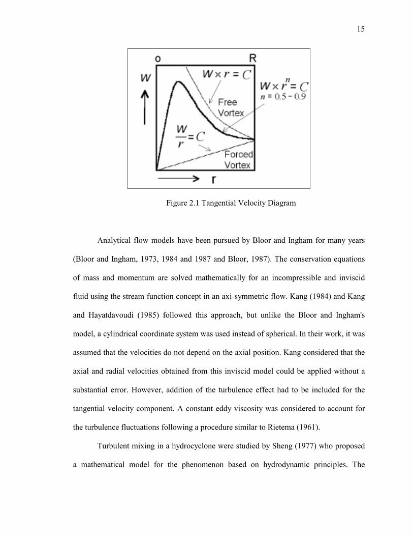
Based on the experimental data taken by Kelsall (1952) using an optical method,
many researchers have attempted to correlate the velocity field in the hydrocyclone,
especially the tangential velocity. It can be determined using the following relationship
(Kelsall, 1952, see also Bradley and Pulling, 1959):
ConstantrW n = (2.1)
This implies that the tangential velocity (W) increases as the radius (r) decreases
for positive values of the empirical exponent (n). The exponent, n is usually between 0.5
and 0.9 (Svarovsky, 1984) in the outer vortex, while in the core region it is close to -1
(see Figure 2.1). If n = 1 a free vortex is obtained where a complete conservation of
angular momentum is implied or no viscous effect is considered. However, if n = -1 a
forced vortex or a solid body rotation type is expected. Also, Kelsall's results are an
evidence of the low dependence of the tangential velocity on the axial position.
Page 25
15
Figure 2.1 Tangential Velocity Diagram
Analytical flow models have been pursued by Bloor and Ingham for many years
(Bloor and Ingham, 1973, 1984 and 1987 and Bloor, 1987). The conservation equations
of mass and momentum are solved mathematically for an incompressible and inviscid
fluid using the stream function concept in an axi-symmetric flow. Kang (1984) and Kang
and Hayatdavoudi (1985) followed this approach, but unlike the Bloor and Ingham's
model, a cylindrical coordinate system was used instead of spherical. In their work, it was
assumed that the velocities do not depend on the axial position. Kang considered that the
axial and radial velocities obtained from this inviscid model could be applied without a
substantial error. However, addition of the turbulence effect had to be included for the
tangential velocity component. A constant eddy viscosity was considered to account for
the turbulence fluctuations following a procedure similar to Rietema (1961).
Turbulent mixing in a hydrocyclone were studied by Sheng (1977) who proposed
a mathematical model for the phenomenon based on hydrodynamic principles. The
Page 26
16
purpose of this model is to express turbulence in terms of a dimensionless length. He
evaluated the behavior of the hydrocyclone at different operational conditions using an
overall efficiency concept. An equation to calculate the water recovery from a feed coarse
product stream, for solid separation in a cyclone, was developed by Plitt et al. (1990).
From extensive experimental tests, Colman and Thew (1983) developed some
correlations to predict the migration probability curve, which defines the separation
efficiency for a particular droplet size in a similar way that the grade efficiency does for
solid particles (see 2.1.6 Grade efficiency in Svarovsky, 1984). Later it was found that the
optimized Stokes Number vs. Reynolds Number correlation used in this work was
erroneous (Nezhati in Thew and Smyth, 1997). However, relevant conclusions can be
extracted from this study, such as that the separation efficiency is independent of the split
ratio in the range 0.5 to 10%.
Seyda and Petty (1991) evaluated the separation potential of the cylindrical tail
pipe section. A semi-empirical model to predict the velocity field in a cylindrical
chamber was developed to calculate the particle trajectories, and hence, the grade
efficiency. In the model, the axial velocity was assumed to be independent of the axial
location and a constant eddy viscosity was considered. The theoretical results showed an
optimum split ratio, as opposed to previously reported results, and an increment in the
efficiency when the feed flow rate was increased.
Wolbert et al. (1995) presented an efficient computational model based on the
analysis of the trajectories of the oil droplets. Trajectories were characterized by a
differential equation that combines the models for the three-velocity distributions and the
settling velocity defined by Stokess law. This was achieved using a modified Helmholtz
Page 27
17
law for the tangential velocity, a polynomial correlation for the axial component, and the
continuity equation and wall condition (Kelsall, 1952) for the radial velocity. The
importance of the tail pipe section to the LLHC separation efficiency was confirmed by
comparing the model with experimental results. An extension of Bloor and Ingham
(1973) LLHC model was elaborated by Moraes et al. (1996). The modification takes into
account the difference in the split ratio for liquid-liquid and solid-liquid hydrocyclones.
Although, this model is sophisticated, results shown by the authors, where no reverse
flow is achieved in the parallel section, disagree with published data.
A mechanistic model for the LLHC was developed by Caldentey (2000). The
model is based on the prediction of the velocity field and droplet trajectory analysis. It is
capable of predicting the separation efficiency and pressure drop in the LLHC. The
model was tested against available data in the literature for the tangential, radial and axial
velocity distributions and the pressure drop, showing a good agreement.
CFD Simulations: Numerical simulations or CFD are used widely to investigate
flow hydrodynamics. Erdal (2001) proposed a Mantilla (1998) modified correlation for
the swirl intensity within the GLCC, based on extensive CFD simulations using the
commercial code CFX (1997). As expressed by Hubred et al. (2000), the solution of the
Navier Stokes Equations for simple or complex geometry for non-turbulent flow is
feasible nowadays. But current computational resources are unable to attain the
instantaneous velocity and pressure fields at large Reynolds numbers even for simple
geometries. The reason is that traditional turbulence models, such as k-є, are not suitable
for this complex flow behavior. On the other hand, more realistic and complicated
turbulence models increase the computational times to inconvenient limits.
Page 28
18
The flow in hydrocyclones has been numerically simulated by Rhodes et al.
(1987). A commercial computer code was used to solve the required partial differential
equations which govern the flow. Prandtl mixing-length model was used to account for
the viscous momentum transfer effect. In a further work, Hsieh and Rajamani (1991) (see
also Rajamani and Hsieh, 1988; Rajamani and Devulapalli, 1994) used a modified
Prandtl mixing-length model with a stream function-vorticity version of the equation of
motion. Good agreement with experimental data was observed in this study. The authors
mentioned that the key for success is choosing the appropriate turbulence model and
numerical solution scheme. He et al. (1997) used a three-dimensional model, with a
cylindrical coordinate system and curvilinear grid, for the calculation of the flow field. A
modified k-є turbulence model was proved to achieve good results.
In most of the work reviewed in the previous paragraph, excluding Rhodes et al.
(1987), the models were evaluated through comparison with laser-doppler anemometry
(LDA) data. LDA has many advantages over other techniques. It is not as tedious as the
optical technique and does not cause flow distortion like the Pitot tubes (Chakraborti and
Miller, 1992). Many researchers have used this technique to measure the velocity field
and turbulence intensities (Dabir, 1983; Fanglu and Wenzhen, 1987; Jirun et al., 1990;
Fraser and Abdullah, 1995 and Erdal 2001).
The literature review confirms the need for accurate experimental data utilizing
appropriate sampling procedure and including the measurements of the droplet size
distributions at the inlet and underflow sections, and the need to develop a simple
mechanistic model for the LLHC. These deficiencies are addressed in the present study.
Page 29
19
CHAPTER III
EXPERIMENTAL PROGRAM
This chapter describes the experimental facility, working fluids, definitions of
pertinent separation parameters, and the experimental results of the LLHC.
3.1 Experimental Facility Description
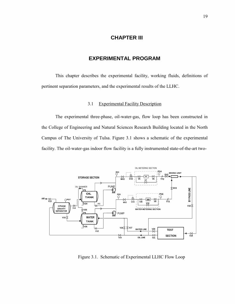
The experimental three-phase, oil-water-gas, flow loop has been constructed in
the College of Engineering and Natural Sciences Research Building located in the North
Campus of The University of Tulsa. Figure 3.1 shows a schematic of the experimental
facility. The oil-water-gas indoor flow facility is a fully instrumented state-of-the-art two-
AIR
V15
3-PHASEGRAVITY
SEPARATORV14
OILTANK
TANKWATER
V23 V21
TEST
SECTION
WATER LINE
OIL LINE
V12
V11
V26
V25
OIL SKIMMER
PG7
PG3
MM
PG5
MM
MIXING UNIT
MV3 CV3 V8
OIL METERING SECTION
WATER METERING SECTION
BY PA
SS LI
NE
V13
PUMP
PUMP
V9 TT3
CV2 V5 V7 V6 TT2
DV2
DV3
V18
V19
V20V16 V17
MV2
V10
PG6
PG4
V24
STORAGE SECTION
Figure 3.1. Schematic of Experimental LLHC Flow Loop
Page 30
20
inch flow loop, enabling testing of single separation equipment or combined separation
systems. The test loop consists of four main components: storage and metering section,
LLHC test section, downstream oil-water separation facility, and data acquisition system.
Following is a brief description of these sections.
3.1.1. Storage and Metering Section
Oil and water are stored in two tanks of 400 gallons capacity each. Each tank is
connected to two pumps. The first one is a 3656 model pump, 1x2-8 size, cast iron
construction with bronze impeller, John Crane Type 21 mechanical seal, 10 HP motor
and operates at 3600 rpm. It delivers 25 gpm @ 108 psig. The second one is a 3656
Model pump, 1.5x2-10 size, cast iron construction with bronze impeller, John Crane
Type 21 mechanical seal, 25 HP motor and operates at 3600 rpm. It delivers 110 gpm @
150 psig. Both pumps are equipped with return lines. Each fluid is pumped from the
storage tank to the metering section. The metering section comprises of pressure gages,
control valves, variable speed controllers and state-of-the-art Micromotion® net oil
computers (NOC), which provide the total mass flow rate, water-cut, temperature, and
mixture density. The signals from the flow meters and control valves are fed to the data
acquisition system, which will be described later. Check valves to prevent any back-flow
are installed downstream of the control valves. The metered oil and water are then
combined in a mixing-tee to obtain oil-water dispersion. Additionally, a static mixer is
available in parallel to the mixing-tee for homogenization of the flow.
Page 31
21
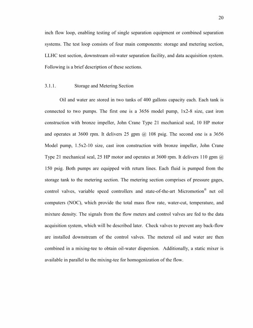
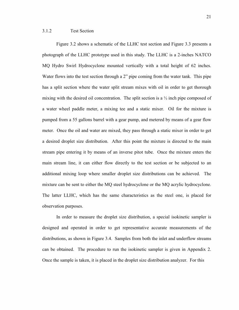
3.1.2 Test Section
Figure 3.2 shows a schematic of the LLHC test section and Figure 3.3 presents a
photograph of the LLHC prototype used in this study. The LLHC is a 2-inches NATCO
MQ Hydro Swirl Hydrocyclone mounted vertically with a total height of 62 inches.
Water flows into the test section through a 2 pipe coming from the water tank. This pipe
has a split section where the water split stream mixes with oil in order to get thorough
mixing with the desired oil concentration. The split section is a ½ inch pipe composed of
a water wheel paddle meter, a mixing tee and a static mixer. Oil for the mixture is
pumped from a 55 gallons barrel with a gear pump, and metered by means of a gear flow
meter. Once the oil and water are mixed, they pass through a static mixer in order to get
a desired droplet size distribution. After this point the mixture is directed to the main
stream pipe entering it by means of an inverse pitot tube. Once the mixture enters the
main stream line, it can either flow directly to the test section or be subjected to an
additional mixing loop where smaller droplet size distributions can be achieved. The
mixture can be sent to either the MQ steel hydrocyclone or the MQ acrylic hydrocyclone.
The latter LLHC, which has the same characteristics as the steel one, is placed for
observation purposes.
In order to measure the droplet size distribution, a special isokinetic sampler is
designed and operated in order to get representative accurate measurements of the
distributions, as shown in Figure 3.4. Samples from both the inlet and underflow streams
can be obtained. The procedure to run the isokinetic sampler is given in Appendix 2.
Once the sample is taken, it is placed in the droplet size distribution analyzer. For this
Page 32
22
Isokinetic Sampler System
Mixing Loop
Oil Tank
Gear Pump
Speed Controller
Water Stream
Oil
Stre
am
Gear Flow Meter
Stat
ic m
ixe
Pressure TransducerThermometer
Pressure Transducer
Acry
lic H
ydro
cycl
one
Stee
l MQ
Hyd
rocy
clon
e
Underflow Stream
Overflow Stream
Overflow Discharge
Oil Stream
Figure 3.2. Schematic of LLHC Test Section
Figure 3.3 Photograph of LLHC Test Section
Page 33
23
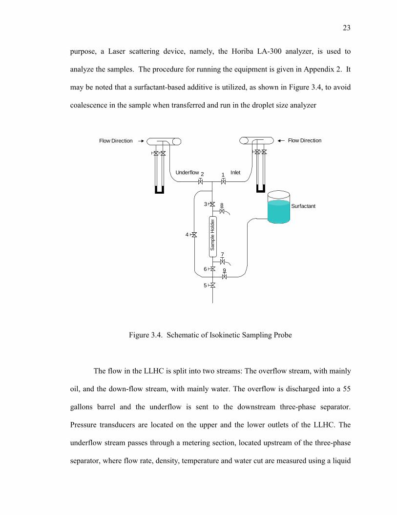
purpose, a Laser scattering device, namely, the Horiba LA-300 analyzer, is used to
analyze the samples. The procedure for running the equipment is given in Appendix 2. It
may be noted that a surfactant-based additive is utilized, as shown in Figure 3.4, to avoid
coalescence in the sample when transferred and run in the droplet size analyzer
Flow Direction
InletUnderflow
Flow Direction
SurfactantSa
mpl
e H
olde
r
12
3
4
5
6
7
9
8
Figure 3.4. Schematic of Isokinetic Sampling Probe
The flow in the LLHC is split into two streams: The overflow stream, with mainly
oil, and the down-flow stream, with mainly water. The overflow is discharged into a 55
gallons barrel and the underflow is sent to the downstream three-phase separator.
Pressure transducers are located on the upper and the lower outlets of the LLHC. The
underflow stream passes through a metering section, located upstream of the three-phase
separator, where flow rate, density, temperature and water cut are measured using a liquid
Page 34
24
Micromotion® coriolis mass flow meter. Due to the small oil concentration in some of
the experiments, a special oil content analyzer is utilized to measure the oil concentration
of the underflow. This equipment is a Horiba OCMA 220 model that uses infrared
spectroscopy technique.
3.1.3 Downstream Oil-Water Separation Section
The 528 gallon three-phase flow separator located downstream of the LLHC test
section operates at 10 psig. It consists of three compartments. In the first compartment the
oil-water mixture is stratified and the oil flows into the second compartment through
flotation. In this compartment, there is a level control system that activates a control
valve discharging the oil into the oil storage tank. The water flows from the first
compartment to the third compartment through a channel located below the second
compartment. In this compartment, there is also a level control system, allowing water to
flow into the water storage tank.
3.1.4 Data Acquisition System
IDM variable speed controllers installed on all the 4 pumps control the oil and
water flow rates into the test section. The flow loop is also equipped with several
temperature sensors and pressure transducers for measurement of the in-situ temperature
and pressure conditions.
All output signals from the sensors, transducers, and metering devices are
collected at a central panel. A state-of-the-art data acquisition system, built using
LabView®, is used to both control the flow in the loop and also to acquire data from
analog signals transmitted from the instrumentation. The program provides variable
Page 35
25
sampling rates. The sampling rate was set at 2 Hz for a 2 minutes sampling period. The
final measured quantity results from an arithmetic averaging of 120 readings, after
steady-state condition is established.
A regular calibration procedure, employing a high-precision pressure pump, is
performed on each pressure transducer at a regular schedule, to guarantee the precision of
measurements. The temperature transducer consists of a Resistance Temperature Detector
(RTD) sensor and an electronic transmitter module.
3.2 Working Fluids
Tap water and mineral oil were chosen and a dye (red) was added to the oil to
improve flow visualization between the phases. The oil has low emulsification, fast
separation, appropriate optical characteristics, non-degrading properties, and is non-
hazardous. A local company (Tulco Oils Inc.) markets the oil. Table 3.1 shows typical
properties of the oil.
During all the experimental runs the average temperature in the flow loop varied
between 700 and 800 F. The average properties of the tap water used are:
Density, ρ= 1.0 ± 0.003 gm/cc
Viscosity, µ = 0.97 ± 0.08 cp.
3.3 Definition of Separation Parameters
Following are the definitions of two important parameters used in this study to
define the total separation efficiency:
Page 36
26
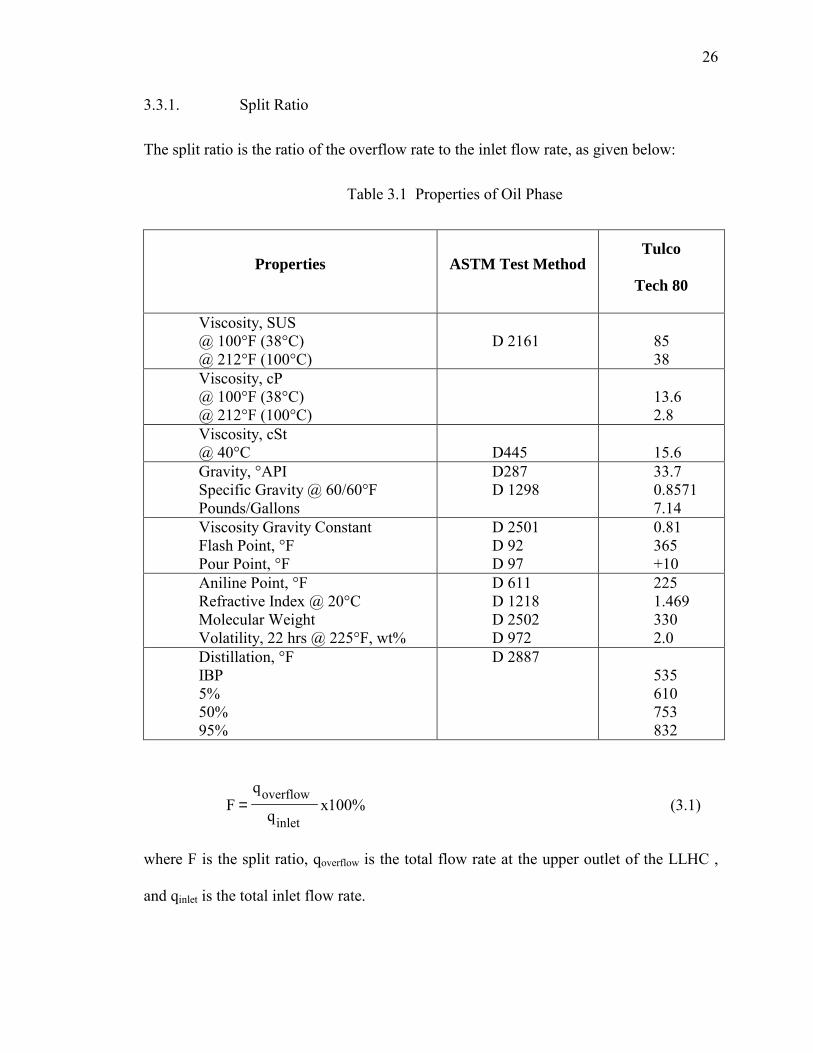
3.3.1. Split Ratio
The split ratio is the ratio of the overflow rate to the inlet flow rate, as given below:
Table 3.1 Properties of Oil Phase
Properties
ASTM Test Method
Tulco
Tech 80
Viscosity, SUS @ 100°F (38°C) @ 212°F (100°C)
D 2161
85 38
Viscosity, cP @ 100°F (38°C) @ 212°F (100°C)
13.6 2.8
Viscosity, cSt @ 40°C
D445
15.6
Gravity, °API Specific Gravity @ 60/60°F Pounds/Gallons
D287 D 1298
33.7 0.8571 7.14
Viscosity Gravity Constant Flash Point, °F Pour Point, °F
D 2501 D 92 D 97
0.81 365 +10
Aniline Point, °F Refractive Index @ 20°C Molecular Weight Volatility, 22 hrs @ 225°F, wt%
D 611 D 1218 D 2502 D 972
225 1.469 330 2.0
Distillation, °F IBP 5% 50% 95%
D 2887 535 610 753 832
%100xq
qF
inlet
overflow= (3.1)
where F is the split ratio, qoverflow is the total flow rate at the upper outlet of the LLHC ,
and qinlet is the total inlet flow rate.
Page 37
27
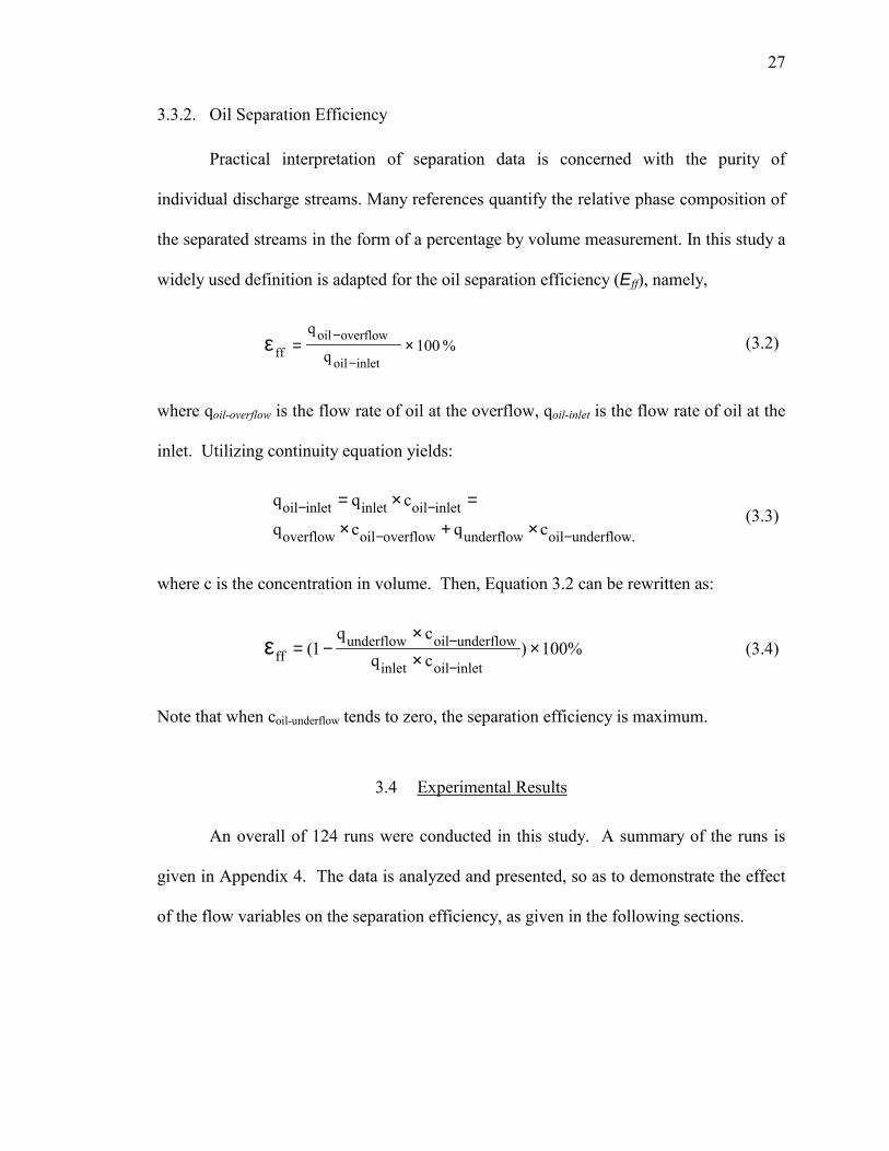
3.3.2. Oil Separation Efficiency
Practical interpretation of separation data is concerned with the purity of
individual discharge streams. Many references quantify the relative phase composition of
the separated streams in the form of a percentage by volume measurement. In this study a
widely used definition is adapted for the oil separation efficiency (Eff), namely,
%100q
q
inletoil
overflowoilff ×=
−
−ε (3.2)
where qoil-overflow is the flow rate of oil at the overflow, qoil-inlet is the flow rate of oil at the
inlet. Utilizing continuity equation yields:
.underflowoilunderflowoverflowoiloverflow
inletoilinletinletoilcqcq
cqq
−−
−−×+×
=×= (3.3)
where c is the concentration in volume. Then, Equation 3.2 can be rewritten as:
%100)cqcq
1(inletoilinlet
underflowoilunderflowff ×
××
−=−
−ε (3.4)
Note that when coil-underflow tends to zero, the separation efficiency is maximum.
3.4 Experimental Results
An overall of 124 runs were conducted in this study. A summary of the runs is
given in Appendix 4. The data is analyzed and presented, so as to demonstrate the effect
of the flow variables on the separation efficiency, as given in the following sections.
Page 38
28
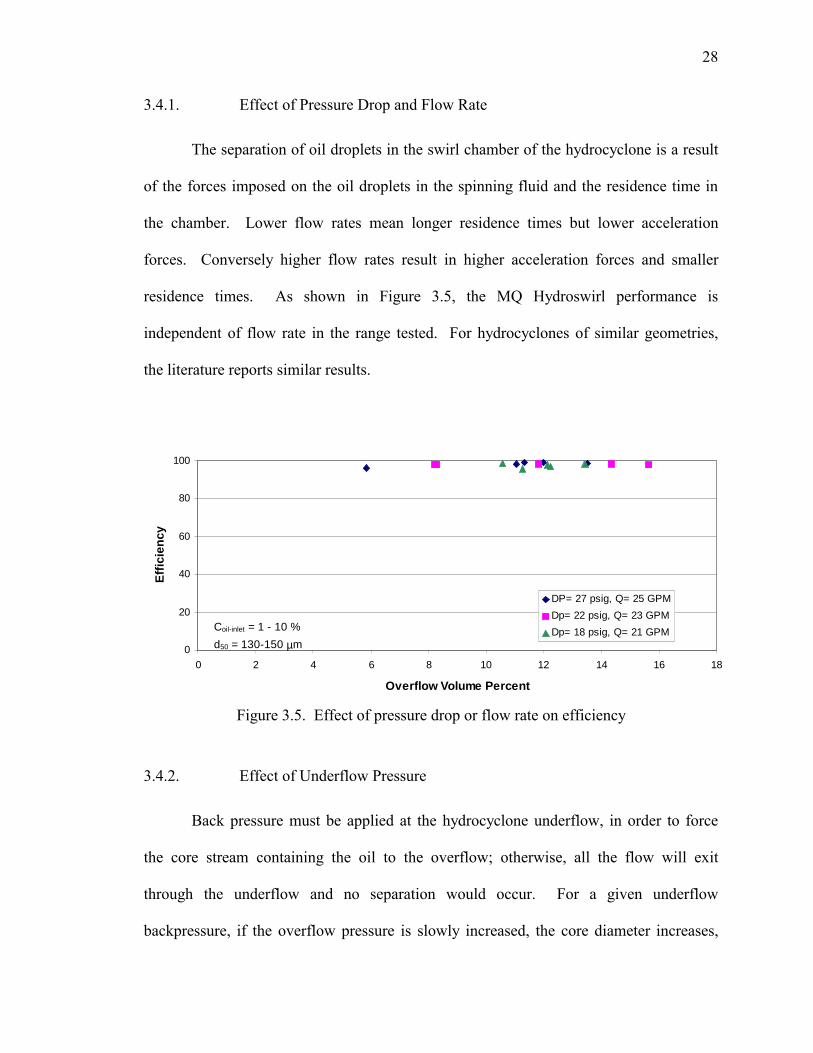
3.4.1. Effect of Pressure Drop and Flow Rate
The separation of oil droplets in the swirl chamber of the hydrocyclone is a result
of the forces imposed on the oil droplets in the spinning fluid and the residence time in
the chamber. Lower flow rates mean longer residence times but lower acceleration
forces. Conversely higher flow rates result in higher acceleration forces and smaller
residence times. As shown in Figure 3.5, the MQ Hydroswirl performance is
independent of flow rate in the range tested. For hydrocyclones of similar geometries,
the literature reports similar results.
0
20
40
60
80
100
0 2 4 6 8 10 12 14 16 18
Overflow Volume Percent
Effic
ienc
y
DP= 27 psig, Q= 25 GPMDp= 22 psig, Q= 23 GPMDp= 18 psig, Q= 21 GPMCoil-inlet = 1 - 10 %
d50 = 130-150 µm
Figure 3.5. Effect of pressure drop or flow rate on efficiency
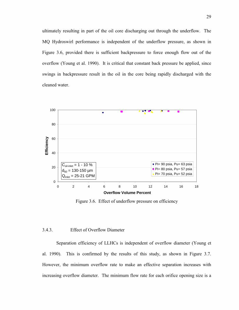
3.4.2. Effect of Underflow Pressure
Back pressure must be applied at the hydrocyclone underflow, in order to force
the core stream containing the oil to the overflow; otherwise, all the flow will exit
through the underflow and no separation would occur. For a given underflow
backpressure, if the overflow pressure is slowly increased, the core diameter increases,
Page 39
29
ultimately resulting in part of the oil core discharging out through the underflow. The
MQ Hydroswirl performance is independent of the underflow pressure, as shown in
Figure 3.6, provided there is sufficient backpressure to force enough flow out of the
overflow (Young et al. 1990). It is critical that constant back pressure be applied, since
swings in backpressure result in the oil in the core being rapidly discharged with the
cleaned water.
0
20
40
60
80
100
0 2 4 6 8 10 12 14 16 18
Overflow Volume Percent
Effic
ienc
y
Pi= 90 psia, Pu= 63 psiaPi= 80 psia, Pu= 57 psiaPi= 70 psia, Pu= 52 psia
Coil-inlet = 1 - 10 %d50 = 130-150 µmQinlet = 25-21 GPM
Figure 3.6. Effect of underflow pressure on efficiency
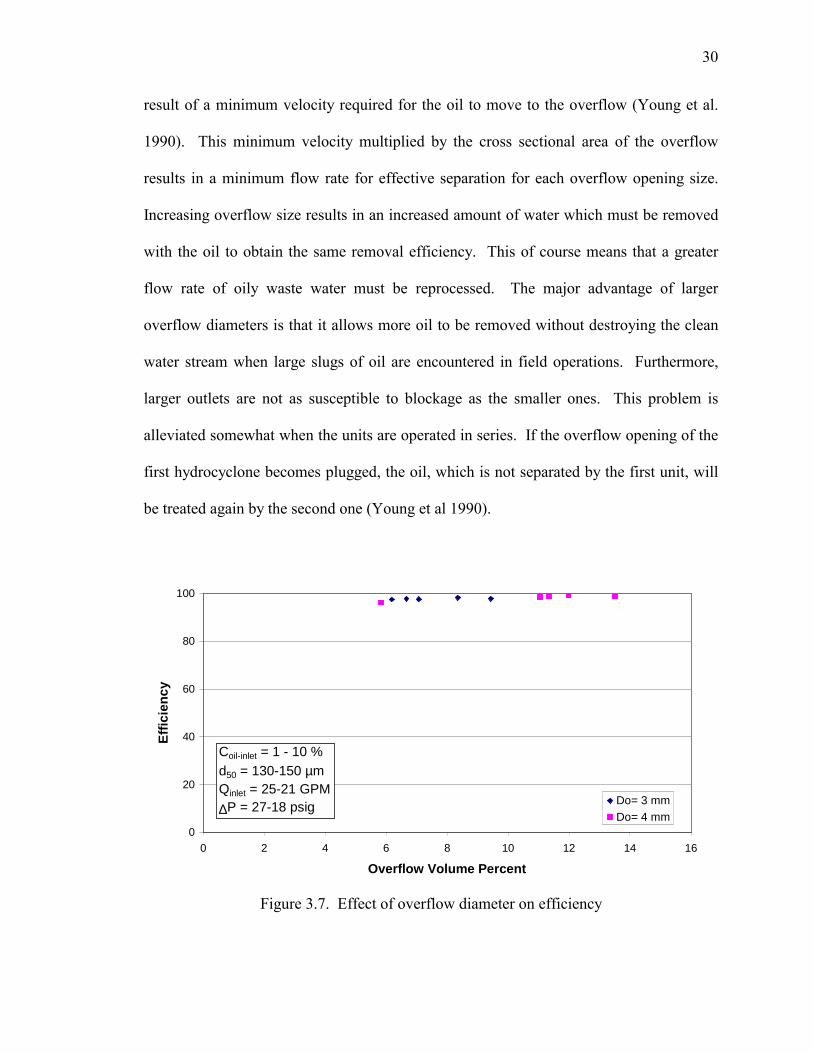
3.4.3. Effect of Overflow Diameter
Separation efficiency of LLHCs is independent of overflow diameter (Young et
al. 1990). This is confirmed by the results of this study, as shown in Figure 3.7.
However, the minimum overflow rate to make an effective separation increases with
increasing overflow diameter. The minimum flow rate for each orifice opening size is a
Page 40
30
result of a minimum velocity required for the oil to move to the overflow (Young et al.
1990). This minimum velocity multiplied by the cross sectional area of the overflow
results in a minimum flow rate for effective separation for each overflow opening size.
Increasing overflow size results in an increased amount of water which must be removed
with the oil to obtain the same removal efficiency. This of course means that a greater
flow rate of oily waste water must be reprocessed. The major advantage of larger
overflow diameters is that it allows more oil to be removed without destroying the clean
water stream when large slugs of oil are encountered in field operations. Furthermore,
larger outlets are not as susceptible to blockage as the smaller ones. This problem is
alleviated somewhat when the units are operated in series. If the overflow opening of the
first hydrocyclone becomes plugged, the oil, which is not separated by the first unit, will
be treated again by the second one (Young et al 1990).
0
20
40
60
80
100
0 2 4 6 8 10 12 14 16
Overflow Volume Percent
Effic
ienc
y
Do= 3 mmDo= 4 mm
Coil-inlet = 1 - 10 %d50 = 130-150 µmQinlet = 25-21 GPM∆P = 27-18 psig
Figure 3.7. Effect of overflow diameter on efficiency
Page 41
31
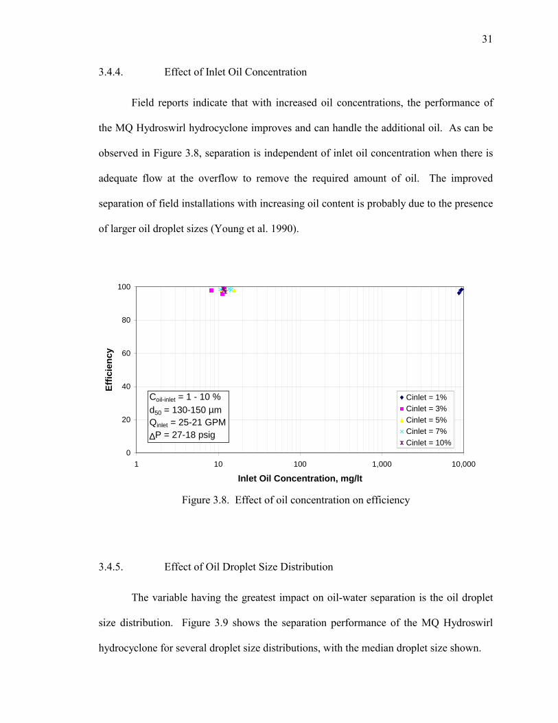
3.4.4. Effect of Inlet Oil Concentration
Field reports indicate that with increased oil concentrations, the performance of
the MQ Hydroswirl hydrocyclone improves and can handle the additional oil. As can be
observed in Figure 3.8, separation is independent of inlet oil concentration when there is
adequate flow at the overflow to remove the required amount of oil. The improved
separation of field installations with increasing oil content is probably due to the presence
of larger oil droplet sizes (Young et al. 1990).
0
20
40
60
80
100
1 10 100 1,000 10,000
Inlet Oil Concentration, mg/lt
Effic
ienc
y
Cinlet = 1%Cinlet = 3%Cinlet = 5%Cinlet = 7%Cinlet = 10%
Coil-inlet = 1 - 10 %d50 = 130-150 µmQinlet = 25-21 GPM∆P = 27-18 psig
Figure 3.8. Effect of oil concentration on efficiency
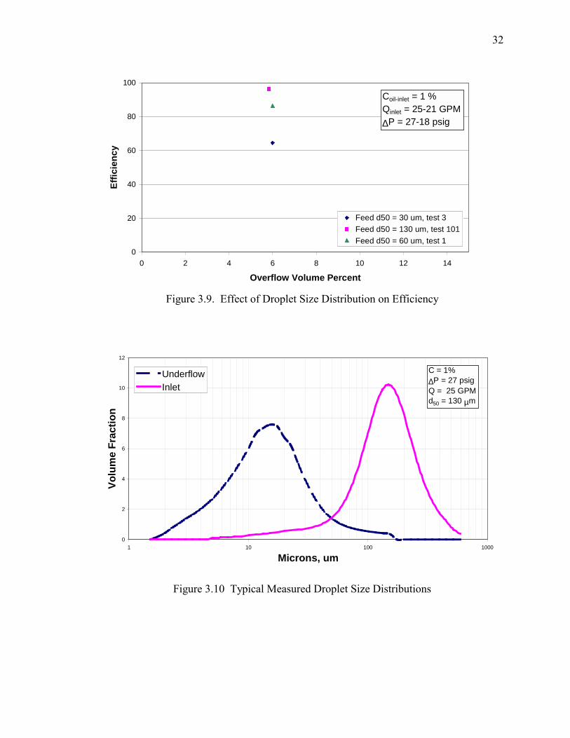
3.4.5. Effect of Oil Droplet Size Distribution
The variable having the greatest impact on oil-water separation is the oil droplet
size distribution. Figure 3.9 shows the separation performance of the MQ Hydroswirl
hydrocyclone for several droplet size distributions, with the median droplet size shown.
Page 42
32
0
20
40
60
80
100
0 2 4 6 8 10 12 14
Overflow Volume Percent
Effic
ienc
y
Feed d50 = 30 um, test 3Feed d50 = 130 um, test 101Feed d50 = 60 um, test 1
Coil-inlet = 1 %Qinlet = 25-21 GPM∆P = 27-18 psig
Figure 3.9. Effect of Droplet Size Distribution on Efficiency
0
2
4
6
8
10
12
1 10 100 1000
Microns, um
Volu
me
Frac
tion
UnderflowInlet
C = 1%∆P = 27 psigQ = 25 GPMd50 = 130 µm
Figure 3.10 Typical Measured Droplet Size Distributions
Page 43
33
Figure 3.9 indicates that the oil separation efficiency increases with increase in
the droplet size. This can be intuitively expected as the larger oil droplets coalesce faster
than the smaller ones.
Typical results for the droplet size distributions in the inlet and underflow streams
are given in Figure 3.10. This figure demonstrates the removal of the large droplets from
the feed stream. Also, the underflow stream contains smaller droplets sizes, as compared
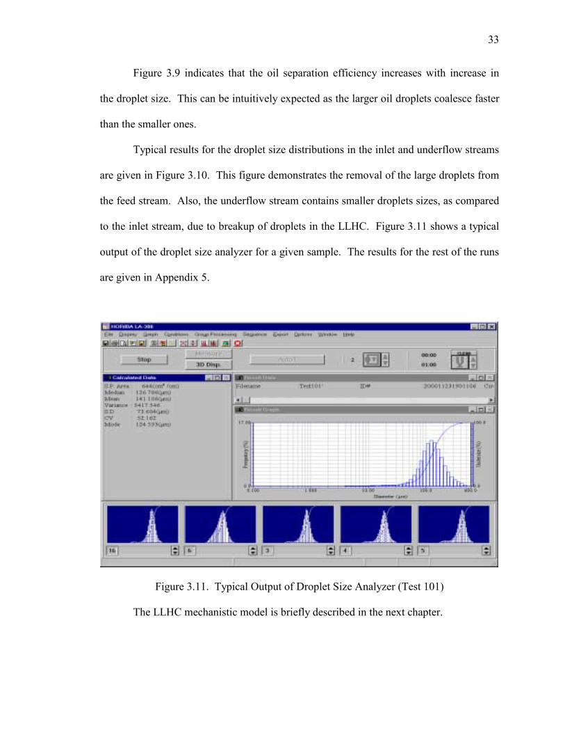
to the inlet stream, due to breakup of droplets in the LLHC. Figure 3.11 shows a typical
output of the droplet size analyzer for a given sample. The results for the rest of the runs
are given in Appendix 5.
Figure 3.11. Typical Output of Droplet Size Analyzer (Test 101)
The LLHC mechanistic model is briefly described in the next chapter.
Page 44
34
CHAPTER IV
LLHC MECHANISTIC MODEL
The LLHC mechanistic model presented in this chapter is a modification of the
original model presented by Caldentey (2000). The main modifications carried out are
improved correlations for the swirl intensity (Ω) that affects the axial and tangential
velocity distributions, for the flow reversal radius (rrev) and for the inlet factor (I). The
following sections provide details of the modified model.
4.1 Swirl Intensity
The swirl intensity is defined as the ratio of the local tangential momentum flux to
the total momentum flux. The swirl intensity equation used by Caldentey (2000), given
below, is a modification of the Mantilla (1998) correlation.
*))tan(2.11(IMM
48.1 15.093.0
2
T
t β+
=Ω
( )
β+
− 12.0
7.016.0
z
35.0
4
T
t )tan(21Dcz
Re1
IMM
21
EXP (4.1)
Based on extensive CFD simulations, Erdal (2001) proposed the following
modification:
*IMM
Re67.093.0
2
T
t13.0
=Ω
Page 45
35
−
7.016.0
z
35.0
4
T
t
Dcz
Re1
IMM
21
EXP (4.2)
The present study utilizes a combination of Caldentey and Erdal correlations, as
given below:
*))tan(2.11(IMM
Re49.0 15.093.0
2
T
t118.0 β+
=Ω
( )( )
β+
− 12.0
7.016.0
z
35.04
T
t tan21Dcz
Re1
IMM
21
EXP (4.3)
where Mt/MT is the ratio of the momentum flux at the inlet slot to the axial momentum
flux at the characteristic diameter position, calculated as:
is
c
cc
isc
avc
is
T
t
AA
A/mA/m
UmVm
MM
=ρρ
==
(4.4)
The variables in the above equations are: Ω is the swirl intensity, Re is the
Reynolds number, β is the semi-angle of the conical sections, Dc is the characteristic
diameter of the LLHC (measured where the angle changes from the reducing section to
the tapered section in the Colman and Thews Design, and at the top diameter of the 3º
tapered section of the Youngs Design), z is the axial position starting from Dc, Vis is the
velocity at the inlet, Uavc is the average axial velocity at Dc, m is the mass flow rate, Ac is
the cross sectional area at Dc and Ais is the inlet cross sectional area.
The Reynolds number is defined in the same way as for pipe flow with the
caution that it refers to a given axial position, yielding:
Page 46
36
c
zavzcz
DURe
µρ
= (4.5)
where µc is the viscosity of the continuous fluid.
The inlet factor, I, as suggested by Erdal (2001), is defined as:
−−=
2n
EXP1I (4.6)
where n = 1.5 for twin inlets and n = 1 for involute single inlet. Note that Caldentey
(2000) utilized an inlet factor defined as I = 1 EXP(-n).
4.2 Velocity Field
The swirl intensity is related, by definition, to the local axial and tangential
velocities. Therefore, it is assumed that once the swirl intensity is predicted for a specific
axial location, it can be used to predict the velocity profiles. Both the tangential and axial
velocities are calculated following a similar procedure as proposed by Mantilla (1998).
The radial velocity, which is the smallest in magnitude, is computed considering the
continuity equation and the wall effect.
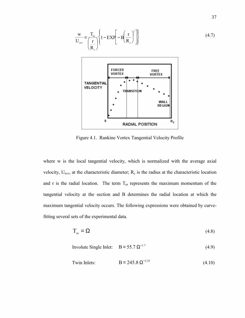
Tangential Velocity: It has been confirmed experimentally that the tangential
velocity is a combination of a forced vortex near the hydrocyclone axis, and a free-like
vortex in the outer wall region, neglecting the effect of the wall boundary layer, as shown
in Figure 4.1. This type of behavior is known as a Rankine Vortex.
Algifri et al. (1988) proposed the following equation for the tangential velocity
profile:
Page 47
37
−−
=
2
c
c
m
avc Rr
BEXP1
Rr
TUw (4.7)
Figure 4.1. Rankine Vortex Tangential Velocity Profile
where w is the local tangential velocity, which is normalized with the average axial
velocity, Uavc, at the characteristic diameter; Rc is the radius at the characteristic location
and r is the radial location. The term Tm represents the maximum momentum of the
tangential velocity at the section and B determines the radial location at which the
maximum tangential velocity occurs. The following expressions were obtained by curve-
fitting several sets of the experimental data.
Ω=mT (4.8)
Involute Single Inlet: 7.17.55B −Ω= (4.9)
Twin Inlets: 35.28.245B −Ω= (4.10)
Page 48
38
It can be seen that the above equations are only functions of the swirl intensity, Ω.
Thus, for a given axial position, the tangential velocity is only function of the radial
location and the swirl intensity.
Axial Velocity: In swirling flow the tangential motion gives rise to centrifugal
forces which in turn tend to move the fluid toward the outer region (Algifri 1988). Such a
radial shift of the fluid results in a reduction of the axial velocity near the axis, and when
the swirl intensity is sufficiently high, reverse flows can occur near the axis. This
phenomenon causes a characteristic reverse flow around the LLHC axis, which allows
the separation of the different density fluids.
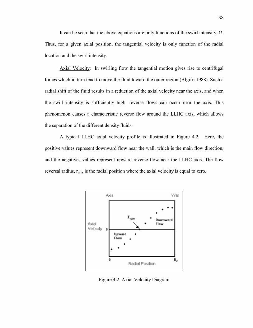
A typical LLHC axial velocity profile is illustrated in Figure 4.2. Here, the
positive values represent downward flow near the wall, which is the main flow direction,
and the negatives values represent upward reverse flow near the LLHC axis. The flow
reversal radius, rrev, is the radial position where the axial velocity is equal to zero.
Figure 4.2 Axial Velocity Diagram
Page 49
39
To predict the axial velocity profile, a third-order polynomial equation is used
with the proper boundary conditions. The general form is as follows:
432
23
1 ararara)r(u +++= (4.11)
where a1, a2, a3 and a4 are constants. The boundary conditions considered are:
1. 0dr
)Rr(du z ==
the velocity is maximum at the wall;
2. 0)rr(u rev == zero velocity at the location of reverse flow, rrev;
3. 0dr
)0r(du=
= the velocity is symmetric about the LLHC axis; and
4. 2zc
R
0 avzc RUrdr)r(u2 z πρ=πρ mass conservation.
Substituting the boundary conditions in Equation (4.11), yields the axial velocity
profile, which is a function of the swirl intensity, Ω only:
1C7.0
2
Rr
C3
3
Rr
C2
Uu
zzavz++
−
= (4.12)
7.0Rr
23Rr
Czz
rev2
rev −
−
= (4.13)
3.0rev 21.0Rr
zΩ= (4.14)
Several assumptions are implicit in these equations. First, an axisymetric
geometry is imposed. Then, the effects of the boundary layer are neglected, and finally
the mass conservation balance does not consider the split ratio. The last assumption can
Page 50
40
be considered a good approximation for small values of split ratios used in the LLHC,
usually less than 10%.
Radial Velocity: The radial velocity, v, of the continuous phase is very small, and
has been neglected in many studies. In our case, in order to track the position of the
droplets in cylindrical and conical sections, the continuity equation and wall conditions
suggested by Kelsall (1952) and Wolbert (1995) are used for the radial velocity profile,
yielding:
utan(βtRrv
z
−= (4.15)
The radial velocity is a function of the axial velocity and geometrical parameters. In the
particular case of cylindrical sections, where tan(β) = 0, the radial velocity, v, is equal to
0.
4.3 Droplet Trajectories
The droplet trajectory model is developed using a Lagrangian approach in which
single droplets are traced in a continuous liquid phase. The droplet trajectory model
utilizes the flow field presented in the previous section.
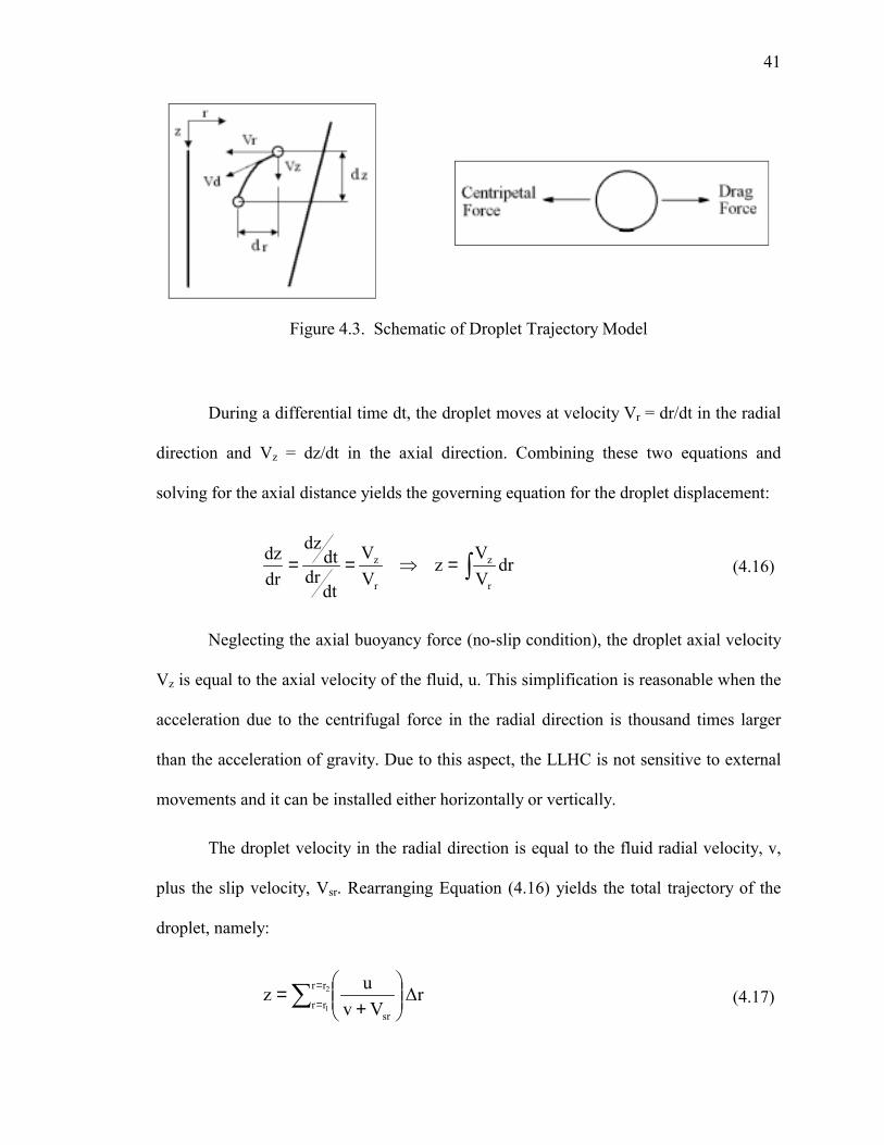
Figure 4.3 presents the physical model. A droplet is shown at two different time
instances, t and t + dt. The droplet moves radially with a velocity Vr and axially with Vz.
It is assumed that in the tangential direction the droplet velocity is the same as the
continuous fluid velocity, as no force acts on the droplet in this direction. Therefore, the
trajectory of the droplet is presented only in two dimensions, namely r and z.
Page 51
41
Figure 4.3. Schematic of Droplet Trajectory Model
During a differential time dt, the droplet moves at velocity Vr = dr/dt in the radial
direction and Vz = dz/dt in the axial direction. Combining these two equations and
solving for the axial distance yields the governing equation for the droplet displacement:
=== drVVz
VV
dtdr
dtdz
drdz
r
z
r
z (4.16)
Neglecting the axial buoyancy force (no-slip condition), the droplet axial velocity
Vz is equal to the axial velocity of the fluid, u. This simplification is reasonable when the
acceleration due to the centrifugal force in the radial direction is thousand times larger
than the acceleration of gravity. Due to this aspect, the LLHC is not sensitive to external
movements and it can be installed either horizontally or vertically.
The droplet velocity in the radial direction is equal to the fluid radial velocity, v,
plus the slip velocity, Vsr. Rearranging Equation (4.16) yields the total trajectory of the
droplet, namely:
∆rVv
uz 2
1
rr
rrsr
=
=
+= (4.17)
Page 52
42
The only unknown parameter in Equation (4.17) is the slip velocity, which can be
solved from a force balance on the droplet in the radial direction, as shown Figure 4.3.
Assuming a local equilibrium momentum yields:
4πdVρC
21
6πd
rw)ρ(ρ
22
srcD
32
dc =− (4.18)
where the left side of the equation is the centripetal force, and the right side is the drag
force. Solving for the radial slip velocity, results in:
21
D
2
c
dcsr C
dr
wρρρ
34V
−= (4.19)
where d is the droplet diameter, ρd is the density of the dispersed phase, ρc is the density
of the continuous phase and CD is the drag coefficient calculated using the following
relationship (Morsi and Alexander, 1972 and Hargreaves, 1990):
2d
3
d
21D Re
bReb
bC ++= (4.20)
where the coefficients b are dependent on the Reynolds Number of the droplets,
defined as:
c
src VdRed µ
ρ= (4.21)
The values for the b coefficients, as functions of the range of Red, are shown in Table
4.1:
Table 4.1. Drag Coefficient Constants
Page 53
43
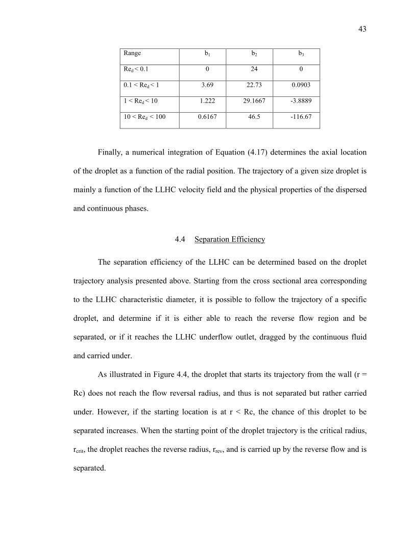
Range b1 b2 b3
Red < 0.1 0 24 0
0.1 < Red < 1 3.69 22.73 0.0903
1 < Red < 10 1.222 29.1667 -3.8889
10 < Red < 100 0.6167 46.5 -116.67
Finally, a numerical integration of Equation (4.17) determines the axial location
of the droplet as a function of the radial position. The trajectory of a given size droplet is
mainly a function of the LLHC velocity field and the physical properties of the dispersed
and continuous phases.
4.4 Separation Efficiency
The separation efficiency of the LLHC can be determined based on the droplet
trajectory analysis presented above. Starting from the cross sectional area corresponding
to the LLHC characteristic diameter, it is possible to follow the trajectory of a specific
droplet, and determine if it is either able to reach the reverse flow region and be
separated, or if it reaches the LLHC underflow outlet, dragged by the continuous fluid
and carried under.
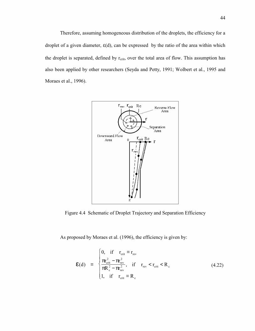
As illustrated in Figure 4.4, the droplet that starts its trajectory from the wall (r =
Rc) does not reach the flow reversal radius, and thus is not separated but rather carried
under. However, if the starting location is at r < Rc, the chance of this droplet to be
separated increases. When the starting point of the droplet trajectory is the critical radius,
rcrit, the droplet reaches the reverse radius, rrev, and is carried up by the reverse flow and is
separated.
Page 54
44
Therefore, assuming homogeneous distribution of the droplets, the efficiency for a
droplet of a given diameter, ε(d), can be expressed by the ratio of the area within which
the droplet is separated, defined by rcrit, over the total area of flow. This assumption has
also been applied by other researchers (Seyda and Petty, 1991; Wolbert et al., 1995 and
Moraes et al., 1996).
Figure 4.4 Schematic of Droplet Trajectory and Separation Efficiency
As proposed by Moraes et al. (1996), the efficiency is given by:
=
<<π−ππ−π
=
=ε
ccrit
ccritrev2rev
2c
2rev
2crit
revcrit
Rrif,1
Rrrif,rRrr
rrif,0
)d( (4.22)
Page 55
45
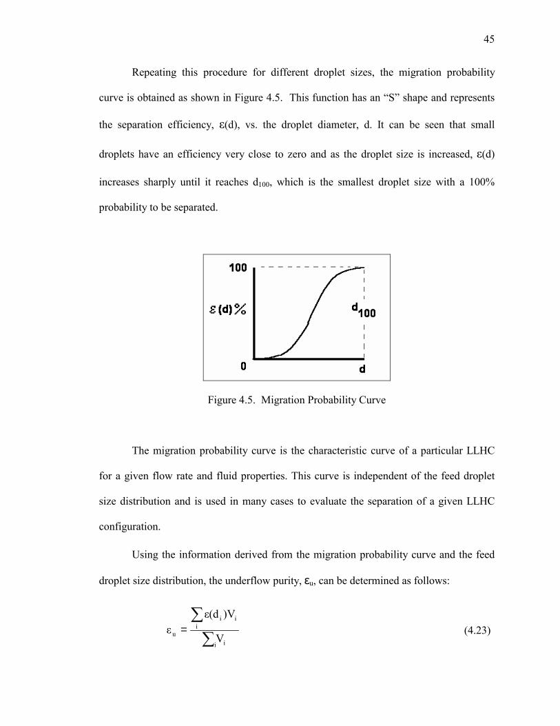
Repeating this procedure for different droplet sizes, the migration probability
curve is obtained as shown in Figure 4.5. This function has an S shape and represents
the separation efficiency, ε(d), vs. the droplet diameter, d. It can be seen that small
droplets have an efficiency very close to zero and as the droplet size is increased, ε(d)
increases sharply until it reaches d100, which is the smallest droplet size with a 100%
probability to be separated.
Figure 4.5. Migration Probability Curve
The migration probability curve is the characteristic curve of a particular LLHC
for a given flow rate and fluid properties. This curve is independent of the feed droplet
size distribution and is used in many cases to evaluate the separation of a given LLHC
configuration.
Using the information derived from the migration probability curve and the feed
droplet size distribution, the underflow purity, εu, can be determined as follows:
=
i i
iii
u V
)Vε(dε (4.23)
Page 56
46
where εu is expressed in %, and Vi is the percentage volumetric fraction of the oil
droplets of diameter di. The underflow purity is the parameter that quantifies the LLHC
capacity to separate the dispersed phase from the continuous one.
4.5 Pressure Drop
The pressure drop from the inlet to the underflow outlet is calculated using a
modification of the Bernoullis Equation:
Lsing)hh(U21
PV21
P cfcfc2UcU
2iscis θρ++ρ+ρ+=ρ+ (4.24)
where ρc is the density of the continuous phase; Pis and Pu are the inlet and outlet
pressures, respectively; Vis is the average inlet velocity and Uu is the underflow average
axial velocity; L is the hydrocyclone length, θ is the angle of the LLHC axis with the
horizontal; hcf corresponds to the centrifugal force losses and hf is the frictional losses.
The frictional losses are calculated similar to that of pipe flow:
2)z(V
)z(Dz
)z(f)z(h2r
f
∆= (4.25)
where f is the friction factor and Vr is the resultant velocity.
In the case of conical sections, all parameters in Equation (4.25) change with the
axial position, z. The conical section is divided into m segments and assuming
cylindrical geometry in each segment, the frictional losses can be considered as the sum
of the losses in all the m segments, as follows.
Page 57
47
( )2
V
2DD
∆zzfh
)2
Z)1n2(at(
2rm
1n n1n)conical(f
∆−
= − += (4.26)
The resultant velocity, Vr, is calculated as the vector sum of the average axial and
tangential velocities. The annular downward flow region is only considered, as presented
in the following set of equations:
2Z
2Z
2R WU)z(V += (4.27)
= 2π
0
R
r
2π
0
R
rz z
rev
z
rev
rdrdφ
WrdrdφW (4.28)
For simplification purposes, the average axial velocity in Equation (4.27), Uz, is
calculated assuming plug flow, namely, Uz is equal to the total flow rate over the annular
area from the wall to the reverse radius, rrev. The Moody friction factor is calculated using
Halls Correlation (Hall, 1957).
+
ε+=
3/164
)zRe(10
)z(D10x210055.0)z(f (4.29)
where ε is the pipe roughness and Re is the Reynolds Number, calculated based on the
resultant velocity computed in Equation (4.27).
The centrifugal losses are the most important ones in Equation (4.24), and account
for most of the total pressure drop in the LLHC. They are calculated using the following
expression:
Page 58
48
= u
rev
R
r
2u
cf drr
)r()nW(h (4.30)
where Wu is calculated from Equation (4.28) at the underflow outlet and the centrifugal
force correction factor, n = 2 for twin inlets, and n = 3.2 for involute single inlet.
The centrifugal force correction factor compensates for the use of Bernoullis
Equation under a high rotational flow condition. Its meaning is similar to the kinetic
energy coefficient used to compensate for the non-uniformity of the velocity profile in
pipe flow (Munson et al., 1994). Rigorously, the Bernoulli equation is valid for a
streamline and the summation of the pressure, the hydrostatic and the kinetic terms can
only be considered constant in all the flow field if the vorticity is equal to zero.
4.6 LLHC Mechanistic Model Code
In order to validate and compare the LLHC mechanistic model with the
experimental data, a computer code originally developed by Caldentey (2000) was
modified in this study to include the improvements made in the mechanistic model, as
described in this chapter. The program was developed in Excel/Visual Basic Application.
Excel/VBA platform can provide advantages such as user-friendly interface forms and
easiness to manipulate the output data.
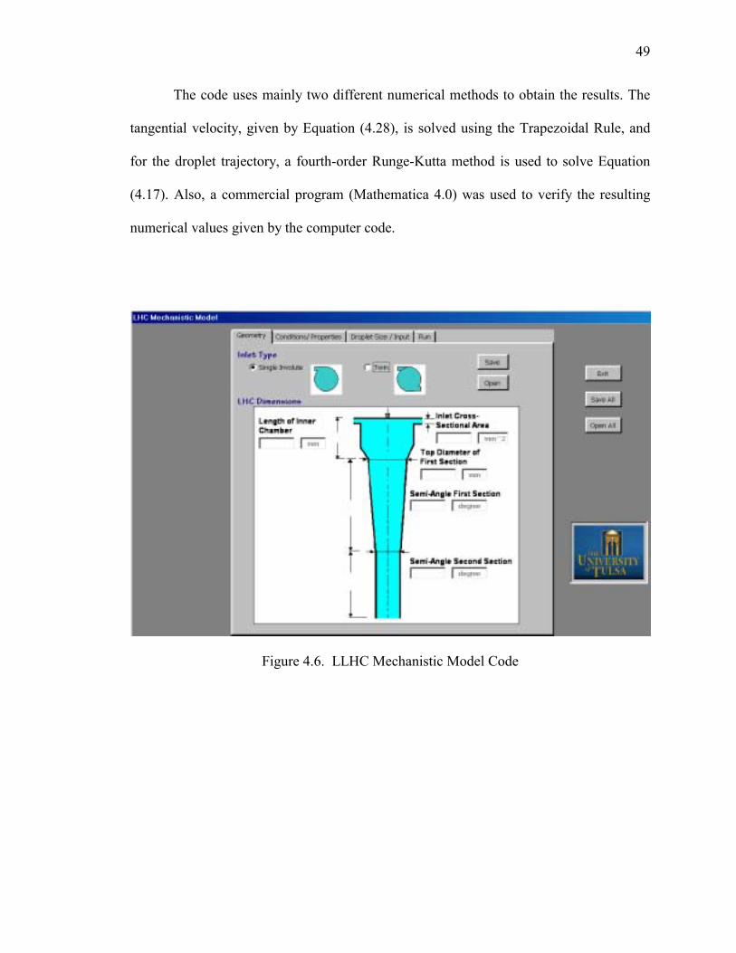
Figure 4.6 presents the multipage form used in the computer code where the user
can interact with the program. All the input data such as geometry, operating conditions,
fluid properties and feed droplet size distribution are located in this form in separate
folders. Buttons to run the program, as well as save and open input cases, are also
included. All the results of the program are presented in the worksheets of the Excel
Application.
Page 59
49
The code uses mainly two different numerical methods to obtain the results. The
tangential velocity, given by Equation (4.28), is solved using the Trapezoidal Rule, and
for the droplet trajectory, a fourth-order Runge-Kutta method is used to solve Equation
(4.17). Also, a commercial program (Mathematica 4.0) was used to verify the resulting
numerical values given by the computer code.
Figure 4.6. LLHC Mechanistic Model Code
Page 60
50
CHAPTER V
RESULTS AND DISCUSSION
This chapter presents comparison between the LLHC mechanistic model
predictions and experimental data taken either at the present study or from the literature.
Comparisons are made for global separation efficiency, migration probability, swirl
intensity, velocity profiles and pressure drop.
5.1 Global Separation Efficiency
Both the underflow purity and the migration probability curve predicted by the
model are evaluated through comparisons with experimental data. Table 5.1 summarizes
the results for efficiency obtained when the model is compared with experimental data
from the present study, and Table 5.2 shows a comparison with literature experimental
data reported by Caldentey (2000). In Table 5.2, cases 9 to 22 are part of the set of
experiments published by Colman et al. (1980). These experimental data sets are for the
LLHC configuration given in Table 5.3. The characteristic diameter and operational
conditions are reported in Table 5.2.
As can be seen from both tables 5.1 and 5.2, the model predictions are in excellent
agreement with both data sets. The results are also plotted in Figures 5.1 and 5.2,
respectively.
Page 61
51
Table 5.1. Efficiency Comparison with Present Study Data.
Test Pinlet ∆P Temp. Q inlet Oilinlet Split Ratio Reject Dia. Experim. Model
(#) dmin (µm) d50(µm) dmax(µm) (psia) (psi) (ºF) (GPM) (%) (%) (mm) Efficien. Efficien.1 2.3 51 200 92 27 80 25 1 6 3 87 893 1.7 33 116 71 18 80 21 1 6 3 64 666 1.9 53 200 91 26 79 25 3 6 3 87 908 1.7 31 116 70 18 79 21 3 5 3 60 6211 1.9 56 200 91 27 80 25 5 12 3 89 9113 1.7 33 133 71 18 80 21 5 6 3 63 6616 1.9 62 229 90 28 79 25 7 14 3 92 9318 1.7 30 116 70 19 80 22 7 9 3 64 6821 2.3 68 262 90 28 72 25 10 11 3 96 9623 1.7 37 133 70 19 72 22 10 12 3 73 73
101 5.1 133 592 90 27 77 25 1 6 4 96 96102 5.1 133 517 79 23 77 23 1 8 4 98 98103 7.7 185 592 70 19 78 22 1 13 4 99 98106 11.6 140 592 90 27 78 26 3 12 4 99 99111 5.9 133 517 90 27 79 26 5 11 4 98 98121 8.8 136 517 90 28 72 25 10 11 4 99 99122 6.7 143 592 79 23 72 23 10 12 4 98 98123 8.8 181 592 70 19 72 22 10 12 4 97 96
Droplet Size Distribution
Table 5.2. Efficiency Comparison with Literature Data.
Case Dc (mm) Flowrate (lpm)
Oil Density (g/cc)
Mean Drop Size
(mc)
Experimental Underflow Purity (%)
Model Underflow Purity (%)
9 30 60 0.87 41 88 8910 30 40 0.84 35 78 7911 30 50 0.84 35 82 8412 30 60 0.84 35 84 8813 30 70 0.84 35 88 9014 58 160 0.84 35 72 6615 58 190 0.84 35 74 7216 58 220 0.84 35 78 7517 58 250 0.84 35 81 7918 58 220 0.84 17 43 4819 58 250 0.84 17 47 5220 58 220 0.84 70 96 9221 58 250 0.84 70 97 9422 58 220 0.87 41 80 80
Table 5.3. Geometrical Parameters, Wolbert et al. (1995)
Case Design Dc(mm) α1 α2 D2 L2 Ds Ls Di
8 IV 20 10º 0.75º 0.5Dc 30Dc 2Dc 2Dc 0.35Dc
Page 62
52
90
91
92
93
94
95
96
97
98
99
100
90 91 92 93 94 95 96 97 98 99 100
Experimental Efficiency (%)
Mod
el E
ffici
ency
(%)
ExperimentalModel
Figure 5.1. Comparison of Model Efficiency with Present Study Experimental Data
0
10
20
30
40
50
60
70
80
90
100
0 10 20 30 40 50 60 70 80 90 100
Experimental Efficiency (%)
Mod
el E
ffici
ency
(%)
ModelExperimental
Figure 5.2. Comparison of Model Efficiency with Literature Experimental Data.
Page 63
53
5.2 Migration Probability
A comparison between the model predictions of the migration probability curve
as compared with experimental data of Colman and Thew (1980) is given in Figure 5.3.
Fair agreement is observed with the data.
5.3 Swirl Intensity
The swirl intensity, which is the ratio of the local tangential momentum flux to
the total momentum flux, can be obtained from Equation (4.1). The experimental data
sets used to compare with the swirl intensity predicted by the model, are given below:
Colmans (1981) work, where the flow field was measured using a Laser
0
10
20
30
40
50
60
70
80
90
100
0 8 16 24 32 40 48 56 64
Droplet Diameter (microns)
Sepa
ratio
n Ef
ficie
ncy
(%)
Experimental Data
Model
Figure 5.3. Migration Probability Comparison, Colman and Thew (1980) Data
Page 64
54
Doppler Anemometer (LDA). In this study four different hydrocyclone
designs were used. However, only designs II, III and IV, as named in the
original work, are used here. The configurations of these hydrocyclones are
shown in Figure 5.4 and the geometrical and operational conditions of each
case study are detailed in Table 5.4 and 5.5, respectively.
The amount of experimental data, presented for each case in the next section,
depends on the availability of axial and tangential velocity measurements at specific axial
locations published by the author. The experimental data shown in Figure 5.5 and Figure
5.8 correspond to cases 2 and 3, respectively, as mentioned in the previous section. All
the data used from design II and III (see Figure 5.4) correspond to the cylindrical sections
with Dc diameter, while the data shown for design IV correspond to the small angle
tapered section.
The results display the swirl intensity versus the dimensionless axial position,
where z is the axial distance from the characteristic diameter, that is the location where
the tapered section begins.
The limited data presented in Figures 5.5 and 5.6 for both cylindrical and low
angle conical sections, respectively, agree well with the model predictions. It has been
experimentally proven by several researchers that the swirl intensity decays exponentially
with axial position due to the wall frictional losses (Chang and Dhir, 1994 and Mantilla,
1998). However, sufficient experimental data is not available to ensure the reliability of
the model to predict the swirl intensity for different angle configurations.
Page 65
55
Figure 5.4 Colman (1981) Designs
Table 5.4. Geometrical Parameters of Colmans Designs (1981) Case Design Dc(mm) L As α1 α2 D2 L2 Ds Ls Du
1 II 58 30Dc 0.125 - 90º 0.5Dc 22Dc - - 0.14Dc
2 III 30 20Dc 0.0625 10º 10º 0.5Dc 21Dc 2Dc 3Dc 0.14Dc
3 IV 30 - 0.0625 10º 0.67º 0.5Dc 21Dc 2Dc 3Dc 0.14Dc
Table 5.5. Operational Conditions of Colmans Designs (1981) Case Design Dc(mm) Flowrate (lpm) T (ºC) F (%)
1 II 58 175 25 10
2 III 30 60 25 10
3 IV 30 60 25 10
where F(%) is the split ratio.
Page 66
56
0
0.5
1
1.5
2
2.5
3
3.5
0 200 400 600 800 1000 1200 1400
Z (mm)
Swirl
Inte
nsity
Experimental DataModel
Figure 5.5. Swirl Intensity Comparison (Colman and Thew (1980), Case 2 Data)
0
0.5
1
1.5
2
2.5
3
3.5
0 200 400 600 800 1000 1200 1400
Z (mm)
Swirl
Inte
nsity
Experimental DataModel
Figure 5.6. Swirl Intensity Comparison (Colman and Thew (1980), Case 3 Data)
Page 67
57
5.4 Velocity Profile
The velocity field predicted by the mechanistic model is compared with the same
experimental data sets used for the swirl intensity comparison, namely, cases 2 and 3.
Figures 5.7 and figure 5.8 present the comparison between the experimental data and
model prediction for the tangential velocity at different axial positions. The y-axis of each
chart corresponds to the axis of the LLHC, and the x-axis represents the radial position.
The units used originally were conserved, namely, millimeters per second for the
tangential velocity, and millimeters for the radial position.
The model predicts with acceptable accuracy the tangential velocity at the wall,
the peak velocity and the radius where it occurs. The experimental data and the model
display a Rankine Vortex shape, namely, a combination of forced vortex near the LLHC
axis and a free like vortex at the outer region.
z / Dc = 10.5
0
4000
8000
12000
16000
0 4 8 12 16
Radius (mm)
Tang
entia
l Vel
ocity
(mm
/sec
) Experimental Data
Model
Figure 5.7. Tangential Velocity Comparison (Colman and Thew (1980), Case 2 Data)
Page 68
58
The axial velocities predicted by the model are next compared with the
experimental data in Figure 5.9 and Figure 5.10. The positive values of axial velocities
correspond to downward flow, which is the direction of the main flow, while the negative
values represent the reverse flow. In all the figures, the axial velocity is only shown from
the center line to the wall of the LLHC.
The mechanistic model performance is excellent with respect to the axial velocity
in the downward flow region, and not so good in the reverse flow region. Considering
the calculations that the model follows to compute the separation efficiency, the
prediction of the reverse flow velocity profile is not so important. What is really
important is the prediction of the radius of zero velocity since beyond this point the
droplet is assumed to be separated.
z / Dc = 10.5
0
4000
8000
12000
16000
0 4 8 12
Radius (mm)
Tang
entia
l Vel
ocity
(mm
/sec
)
Experimental Data
Model
Figure 5.8. Tangential Velocity Comparison (Colman and Thew (1980), Case 3 Data)
Page 69
59
z / Dc = 10.5
-7000
0
7000
0 4 8 12 16
Radius (mm)
Tang
entia
l Vel
ocity
(mm
/sec
)Experimental Data
Model
Figure 5.9. Axial Velocity Comparison (Colman and Thew (1980), Case 2 Data)
z / Dc = 10.5
-8000
0
8000
0 4 8 12
Radius (mm)
Tang
entia
l Vel
ocity
(mm
/sec
)
Experimental Data
Model
Figure 5.10. Axial Velocity Comparison (Colman and Thew (1980), Case 3 Data)
Page 70
60
5.5 Pressure Drop
A comparison between the predicted pressure drop and experimental data from
the present study is shown in Figure 5.11.
Figure 5.12 shows the model predictions of pressure drop vs. flow rate as
compared with the experimental data taken by Young et al. (1990). Very good agreement
is observed in both cases.
0
10
20
30
40
50
60
70
0 10 20 30 40 50 60 70 80 90 100
Pressure Drop, psi
Flow
Rat
e, G
PM
ExperimentalModel
∆P range = 45 -4 psig
Figure 5.11. Pressure Drop vs. Flow Rate Curve (Present Study Data)
5.6 Droplet Trajectories
The prediction of the separation efficiency is based on droplet trajectory analysis.
Once the velocity field of the continuous phase is known, the slip velocity of the droplets
can be calculated and consequently, the trajectory can be determined. Since no data are
available for droplet trajectories, only the prediction of the model will be presented.
Page 71
61
Figures 5.13 and 5.14 demonstrate the droplet trajectory prediction results for conditions
corresponding to test 101.
0
50
100
150
200
250
300
0 50 100 150 200 250
Pressure Drop (psi)
Flow
rate
(lpm
)
Young et al (1990)LLHC Model
F
igure 5.12. Pressure Drop vs. Flow Rate Curve (Young et al. (1990) Data)
As can be seen from Figure 5.13, the larger droplets (130, 60 and 45 micron
diameters) reach the flow reversal radius and are separated easily. However, the smallest
droplets of 35 and 25 micron diameters are not able to reach the reverse flow region, even
when their starting trajectory point is at the wall. Thus, these droplets are carried into the
underflow stream.
Figure 5.14 demonstrates the concept on which the separation efficiency is based
and calculated by the model. A 15 micron droplet is dragged by the fluid when it enters
the top cross sectional area near the wall (r = 25 mm). However, as the droplet is
introduced closer to the LLHC axis, the probability of this droplet to be separated is
Page 72
62
increased. It can be observed that this droplet reaches the flow reversal region when it is
released at a radius equal to 15 mm, which is close to the critical radius, rcrit for this case.
If we consider that the tangential velocity increases considerably as it moves away
from the LLHC wall, and that the axial velocity behaves in an opposite manner, once the
droplet is able to reach these zones of very high centrifugal forces and moderate resident
times, it migrates very fast to the center, reaching the flow reversal region and is
separated. This is the reason why the case study droplet (15µm diameter) passes suddenly
from a starting radius where it cannot be separated, to one where it is easily separated.
0
200
400
600
800
1000
1200
1400
0 5 10 15 20 25 30Radius (mm)
Axi
al P
ositi
on (m
m)
d = 130 um
d = 60
d = 45
d = 35 um d = 25 um
Figure 5.13. Droplet Trajectory Prediction for Test 101 (Droplets Released at the Wall)
Page 73
63
0
200
400
600
800
1000
1200
1400
0 5 10 15 20 25 30Radius (mm)
Axi
al P
ositi
on (m
m)
r = 25 mmr = 20 mmr = 15 mm
r = 14 mm
r = 12 mm
r = 10 mm
Figure 5.14. Droplet Trajectory Prediction for Test 101. (d = 15 µm)
5.7 Droplet Size Distribution
Figures 5.15 and 5.16 show a comparison between the model predictions and
experimental data of the droplet size distribution for runs 101 and 103, respectively. As
shown in the figures, good agreement is observed with experimental results. The model
prediction curves for the underflow droplet size distribution are shifted to the right, which
means that the model predicts efficiency smaller than the experimental one. Also there is
a discontinuity in the model curve because the model doesnt consider either breakup or
coalescence. This means that the smallest droplet that enters the LLHC is also the
smallest one that is found in the underflow stream. On the other hand, the largest droplet
in the underflow stream is the largest droplet with a calculated efficiency below 100%.
Page 74
64
Summary and conclusions of this study are presented in the next chapter along
with recommendations for future investigations.
0
2
4
6
8
10
12
0.1 1 10 100 1000Microns, um
Volu
me
Frac
tion
UnderflowInletLLHC Model
Coil-inlet = 1 %d50 = 130 µmQinlet = 25 GPM∆P = 27 psig
Figure 5.15 Comparison of Droplet Size Distribution Results for Test 101
0
2
4
6
8
10
12
0.1 1 10 100 1000Droplet Size (um)
Volu
me
Frac
tion
(%)
InletUnderflowLLHC Model
Coil-inlet = 1 %d50 = 150 µmQinlet = 21 GPM∆P = 18 psig
Figure 5.16 Comparison of Droplet Size Distribution Results for Test 103
Page 75
65
CHAPTER VI
SUMMARY, CONCLUSIONS AND RECOMMENDATIONS
6.1 Summary and Conclusions
This chapter presents a summary of the contributions and conclusions of the
present study, along with the recommendations for future investigations.
A new facility for testing LLHCs was designed, constructed and installed
in an existing three-phase flow loop. The test section is fully instrumented
to measure the important flow and separation variables, including flow
rates (inlet, underflow and overflow) and the respective oil concentrations;
droplet size distributions (inlet and underflow streams); pressures (inlet
and underflow) and temperature. A mixer bypass loop enables the
generation of a wide range of droplet size distributions. A computer based
data acquisition system was utilized to both control the flow loop and to
acquire the experimental data.
A set of 124 experimental runs was conducted, with inlet total flow rates
between 18 to 26 GPM, inlet oil cuts between 0 to 10%, inlet droplet size
distributions with droplet medians between 30 to 160 microns, inlet
pressures from 60 to 90 psia, underflow pressures between 35 to 63 psia,
temperature between 65ºF 80ºF, and overflow reject diameter of 3mm
Page 76
66
and 4mm. The collected data permitted the calculation of the LLHC
separation efficiency for each of the runs.
A new design for collecting a representative sample for droplet size
distribution measurement was developed and utilized in the experimental
program. The sampler ensures isokinetic conditions and a smooth flow to
the sampling chamber. Also, using a surfactant-based additive,
coalescence is avoided in the sample when transferred and run in the
droplet size distribution analyzer.
The collected data reveals that LLHCs can be used up to 10% inlet oil
concentrations, maintaining high separation efficiency. However, the
performance of the LLHC is best for very low oil concentrations at the
inlet, below 1%. For low concentrations, no emulsification of the mixture
occurs in the LLHC. However, high inlet concentrations, up to 10%,
promote emulsification posing a separation problem in the overflow
stream.
An existing LLHC mechanistic model developed by Caldentey (2000) was
modified and improved. The main modifications carried out are improved
correlations for the swirl intensity (Ω) that affects the axial and tangential
velocity distributions, the flow reversal radius (rrev) and the inlet factor (I).
The model is capable of predicting the hydrodynamic flow field of the
continuous phase within the LLHC. The separation efficiency is
determined based on droplet trajectories, and the inlet-underflow pressure
drop is predicted using an energy balance analysis.
Page 77
67
A user-friendly computer code originally developed by Caldentey (2000)
was modified to include the model improvements. The code provides the
state-of-the-art design tool for the industry.
The prediction of the LLHC model was compared against the data from
both the present study and published data for velocity profiles from the
literature, especially from the Colman and Thew (1990). Good agreement
is obtained between the model predictions and the experimental data with
respect to both separation efficiency (average absolute relative error of
3%) and pressure drop (average absolute relative error of 1.6%).
6.2 Recommendations
The following experimental and theoretical recommendations are suggested for
future studies:
The use of different kind of oils to validate the effects of density
difference, surface tension and viscosity on the performance of the LLHC.
Include the effect of recirculation zones or short circuits at the inlet region.
These two phenomena cause either the return to the main flow of some of
the fluid that flow with the oil core to the overflow outlet, or cause the
feed to flow directly to the reject orifice.
Include the effects of droplet breakup and coalescence in the model.
Visual observations made using the transparent LLHC prototype
confirmed the occurrence of droplet breakup especially for high
Page 78
68
concentrations of oil. Further more, the experimental data of the
underflow droplet size distribution show smaller droplets than the ones
entering the LLHC.
Develop a model for the prediction of the droplet size distribution at the
inlet of the LLHC.
Page 79
69
NOMENCLATURE
A = cross sectional area
B = peak tangential velocity radius factor (Eqs. 4.9 and 4.10)
c = Concentration
CD = drag coefficient
d = droplet diameter
D = diameter
Dc = LLHC characteristic diameter
Eff = Efficiency
f = friction factor
F = Split ratio
h = losses
I = inlet factor
L = length
m = Nº of segments
m = mass flow rate
Mt = momentum flux at the inlet slot
MT = axial momentum flux at the characteristic diameter position
n = centrifugal force correction factor, number of inlets
P = pressure
Q = volumetric flow rate
r = radial position
Page 80
70
R = LLHC radius
Re = Reynolds Number
t = time
Tm = maximum tangential velocity momentum (Eq. 4.8)
u = continuous phase local axial velocity
U = bulk axial velocity
v = continuous phase local radial velocity
V = volumetric fraction / velocity
Vr = droplet radial velocity
Vsr = droplet slip velocity in the radial direction
Vz = droplet axial velocity
w = continuous phase local tangential velocity
W = mean tangential velocity
z = Axial position
Greek Letters:
Ω = swirl intensity
β = taper section semi-angle
ε = efficiency / purity / pipe roughness
θ = axis inclination angle to horizontal
µ = viscosity
ρ = density
Φ = Horizontal plane angle
Page 81
71
Subscripts:
av = average
c = characteristic diameter location / continuous phase
cf = centrifugal
crit = critical
d = dispersed phase / droplet
f = frictional
g = gravity acceleration
i = inlet
is = inlet section
o = overflow
r = resultant
rev = reverse flow
sr = Slip radial velocity
u = underflow
z = axial position
Abbreviations:
CFD = Computational Fluid Dynamics
LDA = Laser Doppler Anemometry
LLHC = Liquid-Liquid Hydrocyclones
NOC = Net Oil Computers
RTD = Resistive Temperature Detector
Page 82
72
REFERENCES
Algifri, A., Bhardwaj, R. and Rao, Y., 1988, Turbulence Measurements in Decaying
Swirl Flow in a Pipe. Applied Scientific Research, Vol. 45, pp. 233-250.
Ali, S., Wesson, G., Petty, C. and Parks, M., 1994, The Use of Small Hydrocyclones for
Produced Water Clarification. Hydrocyclone Development Consortium, Michigan State
University.
Bednarski, S., and Listewnik, J.: "Hydrocyclones for Simultaneous Removal of Oil and
Solid Particle from Ships' Oily Waters", Filtration and Separation, March/April 1988, pp.
92-97.
Beeby, J.P., and Nicol, S.K.: "Concentration of Oil-in-Water Emulsion Using the Air-
Sparged Hydrocyclone", Filtration and Separation, March/April 1993, pp. 141-146.
Bloor, M., 1987, "On Axially Symmetric Flow Models for Hydrocyclones". In 3rd
International Conference on Hydrocyclones, Wood, P. (ed), Elsevier, Oxford, England,
pp. 83-89.
Bloor, M. and Ingham, D., 1973, "Theoretical Investigation of the Flow in a Conical
Hydrocyclone". Trans. Instn. Chem. Engrs., Vol. 51, pp. 36-41.
Bloor, M. and Ingham, D., 1984, "The Influence of Vorticity on the Efficiency of the
Hydrocyclone". In 2nd International Conference on Hydrocyclones, BHRA, Bath,
England, paper B2, pp. 19-21.
Page 83
73
Bloor, M. and Ingham, D., 1987, "The Flow in Industrial Cyclones". Journal of Fluid
Mechanics, Vol. 178, pp. 507-519.
Bradley, D., 1965, "The Hydrocyclone". Pergamon Press.
Bradley, D. and Pulling, D., 1959, "Flow Patterns in the Hydraulic Cyclone and Their
Interpretation in Terms of Performance". Trans. Instn. Chem. Engrs., Vol. 37, pp. 35-44.
Caldentey, J., 2000, A Mechanistic Model for Liquid Hydrocyclones. M.S. Thesis. The
University of Tulsa, U.S.A.
CFX-4.2: Users Guide, 1997, AEA Technology, Computational Fluid Dynamic
Services, 8.19 Harwell, Didcot, Oxfordshire OX11 0RA, United Kingdom.
Chakraborti, N. and Miller, J., 1992, "Fluid Flow in Hydrocyclones: A Critical Review".
Mineral Processing and Extractive Metallurgy Review, Vol. 11, pp. 211-244.
Chang, F and Dhir, V., 1994, Turbulent flow field in tangentially injected swirl flows in
tubes. International Journal of Heat and Fluid Flow, Vol. 15, pp. 346-356.
Choi, M.S, 1990, "Hydrocyclone Produced Water Treatment for Offshore
Developments", SPE 20662.
Colman, D., 1981, The Hydrocyclone for Separating Light Dispersions. Ph.D.
Dissertation. University of Southampton, England.
Colman, D. and Thew, M., 1980, "Hydrocyclone to Give a Highly Concentrated Sample
of a Lighter Dispersed Phase". In International Conference on Hydrocyclones, BHRA,
Cambridge, United Kingdom, paper 15, pp. 209-223.
Colman, D. and Thew, M., 1983, "Correlation of Separation Results From Light
Dispersion Hydrocyclones". Chem. Eng. Res. Des., Vol. 61, pp. 233-240.
Page 84
74
Colman, D. and Thew, M., 1988, "Cyclone Separator". U.S. Patent 4764287.
Colman, D., Thew, M. and Corney, D., 1980, "Hydrocyclones for Oil/Water Separation".
In International Conference on Hydrocyclones, BHRA, Cambridge, United Kingdom,
paper 11, pp. 143-165.
Dabir, B., 1983, "Mean Velocity Measurements in a 3''-Hydrocyclone Using Laser
Doppler Anemometry". Ph.D. Thesis. Michigan State University, Michigan.
Erdal, F., 2001, Local Velocity Measurements and CFD Simulations. Ph.D.
Dissertation. The University of Tulsa, U.S.A.
Fanglu, G. and Wenzhen, L., 1987, "Measurements and Study of Velocity Field in
Various Cyclones by Use of Laser Doppler Anemometry". In 3rd International
Conference on Hydrocyclones, Wood, P. (ed), Elsevier, Oxford, England, pp. 65-74.
Fraser, S. and Abdullah, M., 1995, "LDA Measurement on a Modified Cyclone". ASME
Laser Anemometry, FED-Vol. 229, pp. 395-403.
Gay, J.C., 1987, "Rotary Cyclone Will Omprove Oily Water Treatment and Reduce
Space Requirement/Weight on Offshore Platforms", SPE 16571.
Hall, N., 1957, Thermodynamics of Fluid Flow. Longmans, Green, New York.
Hargreaves, J., 1990, Computing and Measuring the Flowfield in a Deoiling
Hydrocyclone. Ph.D. Thesis. University of Southampton, England.
He, P., Salcudean, M., Branion, R. and Gartshore, I., 1997, "Mathematical Modeling of
Hydrocyclones". In ASME Fluids Engineering Division Summer Meeting, FEDSM97-
3315.
Page 85
75
Hsieh, K. and Rajamani, R., 1991, "Mathematical Model of the Hydrocyclone Based on
Physics of Fluid Flow". AIChE Journal, Vol. 37, No. 5, pp 735-746.
Hubred, G., Mason, A., Parks, S. and Petty, C., 2000, "Dispersed Phase Separations: Can
CFD Help?". Proceeding of ETCE/OMAE Conference, New Orleans, Louisiana.
Jirun, X., Qian, L. and Qui, J., 1990, "Studying the Flow Field in a Hydrocyclone With
no Forced Vortex I, II". Filtration and Separation, July/August, pp. 276-278,
September/October, pp. 356-359.
Johnson, R., Gibson, W.E., and Libby, D.R, 1976, "Performance of Liquid-Liquid
Cyclones", Ind. Eng. Chem. Fundam, Vol. 15, No. 2.
Jones, P.S.: "A Field Comparison of Static and Dynamic Hydrocyclone", SPE Production
and Facilities, May 1993, pp. 84-90.
Kang, J., 1984, "On the Analysis of the Flow and Particle Motion in a Hydrocyclone".
Society of Petroleum Engineers, paper 13407.
Kang, J. and Hayatdavoudi, A., 1985, "Analytical Model Determining the Flow Pattern
and the Distribution of d50 in a Hydrocyclone". Society of Petroleum Engineers, paper
15202.
Kelsall, D., 1952, "A Study of the Motion of Solid Particles in a Hydraulic Cyclone".
Trans. Instn. Chem. Engrs., Vol. 30, pp. 87-108.
Kraipech, W., Chen, W. and Parma, F., 2000, "Prediction of Hydrocyclone Performances
- How Much Can the Models Do?". American Filtration & Separation Society Annual
Conference, Myrtle Beach, SC, March 14-17.
Mantilla, I., 1998, Bubble Trajectory Analysis in Gas-Liquid Cylindrical Cyclone
Separators. M.S. Thesis. The University of Tulsa.
Page 86
76
Meldrum, N., 1988, "Hydrocyclones: A Solution to Produced-Water Tratment". SPE
Production Engineering, November, pp. 669-676.
Moir, D.N.: "Selection and Use of Hydrocylones", The Chemical Engineer, January
1985, pp. 20-27.
Moraes, C., Hackenberg, C., Russo, C. and Medronho, R., 1996, "Theoretical Analysis of
Oily Water Hydrocyclones". In Hydrocyclones 96, Claxton, D., Svarovsky, L. and Thew,
M. (eds), M.E.P., London, England, pp 383-398.
Morsi, S. and Alexander, A., 1971, An Investigation of Particle Trajectories in Two-
Phase Flow Systems. Journal of Fluid Mechanics, Vol. 55, part 2, pp. 193-208.
Munson, B., Young, D. and Okiishi, T., 1994, Fundamentals of Fluid Mechanics. John
Wiley & Sons, Inc. Second Edition.
Plitt, L.R., et al., 1990, "An Improved Method of Calculating the Water-Split in
Hydrocyclones", Minerals Engineering, Vol. 3, No. 5, pp. 533-535.
Rajamani, K. and Devulapalli, B., 1994, "Hydrodynamic Modeling of Swirling Flow and
Particles Classification in Large-Scale Hydrocyclones". KONA Powder and Particle, No.
12, pp. 95-104.
Rajamani, K. and Hsieh, K., 1988, "Hydrocyclone Model: A Fluid Mechanic Approach".
In Society of Mineral Engineers Annual Meeting, Phoenix, Arizona, preprint # 88-163.
Rhodes, N., Pericleous, K. and Drake, S., 1987, "The Prediction of Hydrocyclone
Performance with a Mathematical Model". In 3rd International Conference on
Hydrocyclones, Wood, P. (ed), Elsevier, Oxford, England, pp. 51-58.
Rietema, K., 1961, "Performance and Design of Hydrocyclones - I,II,III,IV". Chemical
Engineering Science, Vol. 15, pp. 298-320.
Page 87
77
Seyda, B. and Petty, C., 1991, "Separation of a Light Dispersion in a Cylindrical Vortex
Chamber". Technical Report No. HDC-R6. Hydrocyclone Development Consortium,
Michigan State University.
Sheng, H.P., "Liquid-Liquid Separation in a Conventional Hydrocyclone", The Canadian
Journal of Chemical Engineering, Vol. 52, August 1974.
Sheng, H.P., 1977, "Separation of Liquids in a Conventional Hydrocyclone", Separation
and Purification Methods, Vol. 6, No. 1, pp. 89-127.
Simkin, D.J., and Olney, R.B., 1956, "Phase Separation and Mass Tranfer in a Liquid-
Liquid Cyclone", AICHE Journal, Vol. 2, No. 4, pp. 545-551.
Smyth, I. and Thew, M., 1996, A Study of the Effect of Dissolved Gas on the Operation
of Liquid-Liquid Hydrocyclones. In Hydrocyclones 96, Claxton, D., Svarovsky, L. and
Thew, M. (eds), M.E.P., London, England, pp 357-368.
Smyth, I., Thew, M., Debenham, P. and Colman, D., 1980, Small-Scale Experiments on
Hydrocyclones for De-watering Light Oils. In International Conference on
Hydrocyclone, Cambridge, England, paper 14, pp. 189-208.
Svarovsky, L., 1984, "Hydrocyclones". Holt, Rinehart & Winston.
Svarovsky, L., 1996, "A Critical Review of Hydrocyclones Models". In Hydrocyclones
96, Claxton, D., Svarovsky, L. and Thew, M. (eds), M.E.P., London, England, pp 17-30.
Syed, K.A., 1994, "The Use of Small Hydrocyclones for Produced Water Clarification",
Michigan State University.
Thew, M., 1986, "Hydrocyclone Redesign for Liquid-Liquid Separation". The Chemical
Engineer, July/August, pp. 17-21.
Page 88
78
Thew, M., Silk, S. and Colman, D., 1980, "Determination and Use of Residence Time
Distribution for Two Hydrocyclones". In International Conference on Hydrocyclones,
BHRA, Cambridge, United Kingdom, paper 16, pp. 225-248.
Thew, M. and Smyth, I., 1997, "Development and Performance of Oil-Water
Hydrocyclone Separators - A Review". In Innovation in Physical Separation
Technologies Conference, Institution of Mining and Metallurgy, Falmouth, United
Kingdom, pp. 77-89.
Thew, M., Wright, C. and Colman, D., 1984, "R.T.D. Characteristics of Hydrocyclones
for the Separation of Light Dispersions". In 2nd International Conference on
Hydrocyclones, BHRA, Bath, England, paper E1, pp. 163-176.
Weispfennig, K. and Petty, C., 1991, "Flow Visualization in a Confined Vortex Flow".
Technical Report No. HDC-R5. Hydrocyclone Development Consortium, Michigan State
University.
Woillez, J., Schummer, P., 1989, "A New High Efficiency Liquid/Liquid Separator",
BHRA, Multi-Phase Flow Proceedings of the 4th International Conference, pp. 117-132.
Wolbert, D., Ma, B. and Aurelle, Y., 1995, "Efficiency Estimation of Liquid-Liquid
Hydrocyclones Using Trajectories Analysis". AIChE Journal, Vol. 41, No. 6, pp 1395-
1402.
Young, G., Taggart, D. and Hild, D., 1993, Improved Understanding of Deoiling
Hydrocyclones Leads to Significant Performance Improvement. Produced in Amoco
Production Company Research Department Tulsa Production Research Division.
Young, G., Walkley, W., Taggart, D., Andrews, S. and Worrel, J., 1990, Oil-Water
Separation Using Hydrocyclones: An Experimental Search for Optimum Dimensions.
American Filtration Society, Advances in Filtration and Separation Technology, Vol.3,
Conference held in Baton Rouge, Louisiana.
Page 89
79
APPENDICES
APPENDIX 1
MQ HYDROSWIRL LLHC SPECIFICATIONS AND DROPLET SIZE
DISTRIBUTIONS
The MQ Hydro-Swirl LLHC has the following specifications:
Design Pressure: 1350 (200 ºF)
Design Temperature: 200 ºF
Flow Rate Capacity: 20-70 GPM
Hydrocyclone Type: MPE MQ Hydro-Swirl
Hydro-Swirl Construction:
Feed, Cone Sections,
Inlet Swirl Chamber: 316L Stainless Steel Constructed to
ANSI B 31.3, & Welded to ASME,
Section IX, with #600 RFWN
Flanges to ANSI 16.5
Oil Reject Orifice: 316L Stainless Steel
Nozzles & Connections: One, 1.0 600# RFWN Inlet; one 1.0
600# RFWN Water Outlet; one, 1.0
600# RFWN Oil Outlet
Page 90
80
Table A1.1. Inlet Droplet Size Distribution Data
Filename test1 Filename test3 Filename test6 Filename test11ID# 2E+14 ID# 2E+14 ID# 2E+14 ID# 2E+14Laser T% 92.7(%) Laser T% 90.2(%) Laser T% 91.5(%) Laser T% 91.2(%)Form of Di Standard Form of Di Standard Form of Di Standard Form of Di StandardCalc. Leve 30 Calc. Leve 30 Calc. Leve 30 Calc. Leve 30DistributionVolume DistributionVolume DistributionVolume DistributionVolumeR.R.Index 1.20-0.00i R.R.Index 1.20-0.00i R.R.Index 1.20-0.00i R.R.Index 1.20-0.00iS.P. Area 1532(cm S.P. Area 2505(cm S.P. Area 1573(cm S.P. Area 1484(cmMedian 51.798(µm) Median 33.503(µm) Median 53.672(µm) Median 56.115(µm)Mean 56.838(µm) Mean 35.761(µm) Mean 58.072(µm) Mean 60.798(µm)Variance 804.371 Variance 291.855 Variance 780.075 Variance 832.272S.D. 28.361(µm) S.D. 17.084(µm) S.D. 27.930(µm) S.D. 28.849(µm)CV 49.899 CV 47.772 CV 48.095 CV 47.451Mode 54.752(µm) Mode 36.426(µm) Mode 55.023(µm) Mode 55.303(µm)Diameter Frequency Undersize (%) Diameter Frequency Undersize (%) Diameter Frequency Undersize (%) Diameter Frequency Undersize (%)
0.115 0 0 0.115 0 0 0.115 0 0 0.115 0 00.131 0 0 0.131 0 0 0.131 0 0 0.131 0 00.15 0 0 0.15 0 0 0.15 0 0 0.15 0 0
0.172 0 0 0.172 0 0 0.172 0 0 0.172 0 00.197 0 0 0.197 0 0 0.197 0 0 0.197 0 00.226 0 0 0.226 0 0 0.226 0 0 0.226 0 00.259 0 0 0.259 0 0 0.259 0 0 0.259 0 00.296 0 0 0.296 0 0 0.296 0 0 0.296 0 00.339 0 0 0.339 0 0 0.339 0 0 0.339 0 00.389 0 0 0.389 0 0 0.389 0 0 0.389 0 00.445 0 0 0.445 0 0 0.445 0 0 0.445 0 00.51 0 0 0.51 0 0 0.51 0 0 0.51 0 0
0.584 0 0 0.584 0 0 0.584 0 0 0.584 0 00.669 0 0 0.669 0 0 0.669 0 0 0.669 0 00.766 0 0 0.766 0 0 0.766 0 0 0.766 0 00.877 0 0 0.877 0 0 0.877 0 0 0.877 0 01.005 0 0 1.005 0 0 1.005 0 0 1.005 0 01.151 0 0 1.151 0 0 1.151 0 0 1.151 0 01.318 0 0 1.318 0 0 1.318 0 0 1.318 0 01.51 0 0 1.51 0 0 1.51 0 0 1.51 0 0
1.729 0 0 1.729 0.105 0.105 1.729 0 0 1.729 0 01.981 0 0 1.981 0.185 0.29 1.981 0.111 0.111 1.981 0.106 0.1062.269 0.122 0.122 2.269 0.262 0.552 2.269 0.168 0.279 2.269 0.157 0.2632.599 0.139 0.261 2.599 0.289 0.841 2.599 0.193 0.472 2.599 0.177 0.442.976 0.151 0.412 2.976 0.305 1.146 2.976 0.207 0.679 2.976 0.187 0.6273.409 0.151 0.563 3.409 0.296 1.442 3.409 0.2 0.879 3.409 0.177 0.8043.905 0.15 0.713 3.905 0.288 1.729 3.905 0.19 1.069 3.905 0.166 0.974.472 0.148 0.861 4.472 0.282 2.011 4.472 0.179 1.248 4.472 0.154 1.1245.122 0.148 1.009 5.122 0.284 2.295 5.122 0.169 1.416 5.122 0.143 1.2675.867 0.15 1.159 5.867 0.295 2.59 5.867 0.161 1.578 5.867 0.136 1.4036.72 0.155 1.314 6.72 0.322 2.912 6.72 0.158 1.736 6.72 0.132 1.535
7.697 0.167 1.481 7.697 0.371 3.284 7.697 0.161 1.897 7.697 0.134 1.678.816 0.187 1.668 8.816 0.454 3.738 8.816 0.172 2.069 8.816 0.143 1.813
10.097 0.216 1.884 10.097 0.581 4.318 10.097 0.19 2.258 10.097 0.158 1.97111.565 0.261 2.144 11.565 0.789 5.107 11.565 0.222 2.48 11.565 0.185 2.15613.246 0.337 2.481 13.246 1.13 6.237 13.246 0.278 2.758 13.246 0.232 2.38815.172 0.439 2.92 15.172 1.64 7.877 15.172 0.353 3.111 15.172 0.296 2.68417.377 0.643 3.563 17.377 2.546 10.424 17.377 0.514 3.625 17.377 0.432 3.11619.904 0.975 4.539 19.904 3.862 14.285 19.904 0.78 4.404 19.904 0.658 3.77422.797 1.49 6.029 22.797 5.961 20.247 22.797 1.194 5.598 22.797 1.009 4.78326.111 2.407 8.436 26.111 8.419 28.665 26.111 1.969 7.568 26.111 1.677 6.4629.907 3.832 12.268 29.907 10.861 39.526 29.907 3.227 10.794 29.907 2.779 9.2434.255 5.845 18.113 34.255 12.52 52.046 34.255 5.105 15.899 34.255 4.473 13.71339.234 8.299 26.412 39.234 12.708 64.754 39.234 7.566 23.465 39.234 6.79 20.50344.938 10.7 37.112 44.938 11.322 76.076 44.938 10.214 33.68 44.938 9.447 29.9551.471 12.305 49.417 51.471 8.892 84.968 51.471 12.3 45.98 51.471 11.786 41.73558.953 12.494 61.911 58.953 6.231 91.199 58.953 13.032 59.012 58.953 12.986 54.72167.523 11.188 73.099 67.523 3.96 95.159 67.523 12.084 71.096 67.523 12.542 67.26477.339 8.934 82.034 77.339 2.345 97.504 77.339 9.869 80.964 77.339 10.662 77.92688.583 6.487 88.52 88.583 1.33 98.834 88.583 7.205 88.169 88.583 8.077 86.003101.46 4.402 92.922 101.46 0.744 99.578 101.46 4.817 92.986 101.46 5.573 91.576116.21 2.882 95.805 116.21 0.422 100 116.21 3.036 96.022 116.21 3.6 95.176
133.103 1.874 97.679 133.103 0 100 133.103 1.856 97.878 133.103 2.239 97.416152.453 1.245 98.924 152.453 0 100 152.453 1.138 99.016 152.453 1.386 98.802174.616 0.692 99.616 174.616 0 100 174.616 0.632 99.649 174.616 0.77 99.572
200 0.384 100 200 0 100 200 0.351 100 200 0.428 100
Page 91
81
Table A1.1. Inlet Droplet Size Distribution Data. (Contd).
Filename test13 Filename test16 Filename test18 Filename test21ID# 2.00012E+14 ID# 2.00012E+14 ID# 2.00012E+14 ID# 2.00012E+14Laser T% 89.6(%) Laser T% 87.4(%) Laser T% 83.1(%) Laser T% 85.0(%)Form of DisStandard Form of DisStandard Form of DisStandard Form of DisStandardCalc. Level 30 Calc. Level 30 Calc. Level 30 Calc. Level 30DistributionVolume DistributionVolume DistributionVolume DistributionVolumeR.R.Index 1.20-0.00i R.R.Index 1.20-0.00i R.R.Index 1.20-0.00i R.R.Index 1.20-0.00iS.P. Area 2413(cm S.P. Area 1349(cm S.P. Area 2298(cm S.P. Area 1136(cmMedian 33.209(µm) Median 61.710(µm) Median 33.990(µm) Median 67.772(µm)Mean 36.293(µm) Mean 67.012(µm) Mean 36.849(µm) Mean 74.789(µm)Variance 329.478 Variance 1025.651 Variance 299.31 Variance 1306.505S.D. 18.152(µm) S.D. 32.026(µm) S.D. 17.301(µm) S.D. 36.146(µm)CV 50.014 CV 47.791 CV 46.95 CV 48.33Mode 32.198(µm) Mode 63.028(µm) Mode 32.287(µm) Mode 71.702(µm)Diameter Frequency (%) Undersize (%) Diameter Frequency (%) Undersize (%) Diameter Frequency (%) Undersize (%) Diameter Frequency (%) Undersize (%)
0.115 0 0 0.115 0 0 0.115 0 0 0.115 0 00.131 0 0 0.131 0 0 0.131 0 0 0.131 0 00.15 0 0 0.15 0 0 0.15 0 0 0.15 0 0
0.172 0 0 0.172 0 0 0.172 0 0 0.172 0 00.197 0 0 0.197 0 0 0.197 0 0 0.197 0 00.226 0 0 0.226 0 0 0.226 0 0 0.226 0 00.259 0 0 0.259 0 0 0.259 0 0 0.259 0 00.296 0 0 0.296 0 0 0.296 0 0 0.296 0 00.339 0 0 0.339 0 0 0.339 0 0 0.339 0 00.389 0 0 0.389 0 0 0.389 0 0 0.389 0 00.445 0 0 0.445 0 0 0.445 0 0 0.445 0 00.51 0 0 0.51 0 0 0.51 0 0 0.51 0 0
0.584 0 0 0.584 0 0 0.584 0 0 0.584 0 00.669 0 0 0.669 0 0 0.669 0 0 0.669 0 00.766 0 0 0.766 0 0 0.766 0 0 0.766 0 00.877 0 0 0.877 0 0 0.877 0 0 0.877 0 01.005 0 0 1.005 0 0 1.005 0 0 1.005 0 01.151 0 0 1.151 0 0 1.151 0 0 1.151 0 01.318 0 0 1.318 0 0 1.318 0 0 1.318 0 01.51 0 0 1.51 0 0 1.51 0 0 1.51 0 0
1.729 0.108 0.108 1.729 0 0 1.729 0.127 0.127 1.729 0 01.981 0.181 0.289 1.981 0.101 0.101 1.981 0.193 0.321 1.981 0 02.269 0.243 0.532 2.269 0.146 0.247 2.269 0.237 0.558 2.269 0.135 0.1352.599 0.253 0.785 2.599 0.161 0.408 2.599 0.228 0.786 2.599 0.143 0.2782.976 0.252 1.037 2.976 0.167 0.575 2.976 0.211 0.997 2.976 0.143 0.4213.409 0.231 1.268 3.409 0.155 0.73 3.409 0.182 1.18 3.409 0.129 0.553.905 0.215 1.483 3.905 0.143 0.873 3.905 0.16 1.34 3.905 0.115 0.6644.472 0.203 1.686 4.472 0.131 1.004 4.472 0.144 1.484 4.472 0.101 0.7665.122 0.201 1.887 5.122 0.12 1.124 5.122 0.137 1.621 5.122 0 0.7665.867 0.208 2.095 5.867 0.113 1.237 5.867 0.139 1.76 5.867 0 0.7666.72 0.23 2.325 6.72 0.109 1.346 6.72 0.151 1.911 6.72 0 0.766
7.697 0.274 2.599 7.697 0.11 1.455 7.697 0.18 2.091 7.697 0 0.7668.816 0.35 2.95 8.816 0.116 1.571 8.816 0.234 2.326 8.816 0 0.766
10.097 0.472 3.421 10.097 0.127 1.698 10.097 0.323 2.649 10.097 0 0.76611.565 0.68 4.101 11.565 0.147 1.845 11.565 0.481 3.13 11.565 0 0.76613.246 1.035 5.136 13.246 0.182 2.027 13.246 0.77 3.901 13.246 0.124 0.88915.172 1.598 6.734 15.172 0.229 2.256 15.172 1.256 5.157 15.172 0.155 1.04417.377 2.59 9.324 17.377 0.328 2.584 17.377 2.154 7.311 17.377 0.223 1.26819.904 4.05 13.374 19.904 0.491 3.075 19.904 3.575 10.886 19.904 0.337 1.60522.797 6.424 19.797 22.797 0.739 3.814 22.797 6.01 16.896 22.797 0.511 2.11626.111 9.02 28.817 26.111 1.216 5.03 26.111 8.877 25.773 26.111 0.855 2.97129.907 11.375 40.192 29.907 2.019 7.049 29.907 11.63 37.402 29.907 1.45 4.42134.255 12.712 52.904 34.255 3.308 10.356 34.255 13.361 50.763 34.255 2.448 6.86939.234 12.487 65.391 39.234 5.203 15.559 39.234 13.343 64.106 39.234 4.007 10.87744.938 10.821 76.212 44.938 7.637 23.196 44.938 11.609 75.715 44.938 6.177 17.05351.471 8.368 84.58 51.471 10.218 33.414 51.471 8.912 84.626 51.471 8.754 25.80758.953 5.878 90.458 58.953 12.232 45.646 58.953 6.152 90.779 58.953 11.179 36.98667.523 3.828 94.286 67.523 12.932 58.578 67.523 3.902 94.681 67.523 12.671 49.65777.339 2.382 96.669 77.339 12.037 70.615 77.339 2.344 97.025 77.339 12.673 62.3388.583 1.458 98.126 88.583 9.909 80.524 88.583 1.372 98.398 88.583 11.211 73.541101.46 0.903 99.029 101.46 7.312 87.836 101.46 0.806 99.204 101.46 8.875 82.416116.21 0.58 99.609 116.21 4.935 92.771 116.21 0.487 99.691 116.21 6.412 88.828
133.103 0.391 100 133.103 3.122 95.894 133.103 0.309 100 133.103 4.328 93.156152.453 0 100 152.453 1.915 97.809 152.453 0 100 152.453 2.814 95.971174.616 0 100 174.616 1.175 98.984 174.616 0 100 174.616 1.814 97.785
200 0 100 200 0.653 99.637 200 0 100 200 1.188 98.973
Page 92
82
Table A1.2. Underflow Droplet Size Distribution Data.
Filename underflow-test1 Filename underflow-test3 Filename underflow-test6 Filename underflow-test8ID# 2.00012E+14 ID# 2.00012E+14 ID# 2.00012E+14 ID# 2.00012E+14Laser T% 90.4(%) Laser T% 83.7(%) Laser T% 77.7(%) Laser T% 75.9(%)Form of DisStandard Form of DisStandard Form of DisStandard Form of DisStandardCalc. Leve 30 Calc. Leve 30 Calc. Leve 30 Calc. Leve 30DistributionVolume DistributionVolume DistributionVolume DistributionVolumeR.R.Index 1.20-0.00i R.R.Index 1.20-0.00i R.R.Index 1.20-0.00i R.R.Index 1.20-0.00iS.P. Area 4994(cm S.P. Area 4808(cm S.P. Area 4938(cm S.P. Area 4320(cmMedian 16.098(µm) Median 17.222(µm) Median 16.278(µm) Median 18.965(µm)Mean 17.820(µm) Mean 18.428(µm) Mean 17.791(µm) Mean 26.073(µm)Variance 103.124 Variance 94.44 Variance 95.084 Variance 1093.576S.D. 10.155(µm) S.D. 9.718(µm) S.D. 9.751(µm) S.D. 33.069(µm)CV 56.986 CV 52.736 CV 54.809 CV 126.834Mode 16.304(µm) Mode 21.130(µm) Mode 16.318(µm) Mode 21.211(µm)Diameter Frequency (%) Undersize (%) Diameter Frequency (%) Undersize (%) Diameter Frequency (%) Undersize (%) Diameter Frequency (%) Undersize (%)
0.115 0 0 0.115 0 0 0.115 0 0 0.115 0 00.131 0 0 0.131 0 0 0.131 0 0 0.131 0 00.15 0 0 0.15 0 0 0.15 0 0 0.15 0 0
0.172 0 0 0.172 0 0 0.172 0 0 0.172 0 00.197 0 0 0.197 0 0 0.197 0 0 0.197 0 00.226 0 0 0.226 0 0 0.226 0 0 0.226 0 00.259 0 0 0.259 0 0 0.259 0 0 0.259 0 00.296 0 0 0.296 0 0 0.296 0 0 0.296 0 00.339 0 0 0.339 0 0 0.339 0 0 0.339 0 00.389 0 0 0.389 0 0 0.389 0 0 0.389 0 00.445 0 0 0.445 0 0 0.445 0 0 0.445 0 00.51 0 0 0.51 0 0 0.51 0 0 0.51 0 0
0.584 0 0 0.584 0 0 0.584 0 0 0.584 0 00.669 0 0 0.669 0 0 0.669 0 0 0.669 0 00.766 0 0 0.766 0 0 0.766 0 0 0.766 0 00.877 0 0 0.877 0 0 0.877 0 0 0.877 0 01.005 0 0 1.005 0 0 1.005 0 0 1.005 0 01.151 0 0 1.151 0 0 1.151 0 0 1.151 0 01.318 0 0 1.318 0 0 1.318 0 0 1.318 0 01.51 0 0 1.51 0 0 1.51 0 0 1.51 0 0
1.729 0.112 0.112 1.729 0.168 0.168 1.729 0.15 0.15 1.729 0.163 0.1631.981 0.233 0.346 1.981 0.313 0.481 1.981 0.278 0.428 1.981 0.289 0.4522.269 0.395 0.74 2.269 0.478 0.96 2.269 0.43 0.858 2.269 0.426 0.8792.599 0.526 1.266 2.599 0.585 1.545 2.599 0.539 1.397 2.599 0.508 1.3872.976 0.669 1.935 2.976 0.688 2.232 2.976 0.651 2.048 2.976 0.584 1.9713.409 0.793 2.727 3.409 0.762 2.994 3.409 0.743 2.791 3.409 0.635 2.6063.905 0.949 3.676 3.905 0.857 3.851 3.905 0.864 3.655 3.905 0.704 3.314.472 1.146 4.822 4.472 0.983 4.835 4.472 1.024 4.679 4.472 0.799 4.1095.122 1.414 6.235 5.122 1.166 6 5.122 1.255 5.934 5.122 0.943 5.0515.867 1.777 8.012 5.867 1.425 7.425 5.867 1.581 7.515 5.867 1.153 6.2046.72 2.27 10.283 6.72 1.797 9.222 6.72 2.045 9.56 6.72 1.461 7.665
7.697 2.936 13.219 7.697 2.327 11.548 7.697 2.694 12.254 7.697 1.911 9.5768.816 3.826 17.045 8.816 3.08 14.628 8.816 3.592 15.846 8.816 2.561 12.137
10.097 4.979 22.023 10.097 4.117 18.745 10.097 4.793 20.64 10.097 3.468 15.60511.565 6.509 28.532 11.565 5.589 24.334 11.565 6.421 27.06 11.565 4.77 20.37513.246 7.819 36.351 13.246 7.096 31.43 13.246 7.902 34.962 13.246 6.156 26.53115.172 9.249 45.6 15.172 8.919 40.349 15.172 9.575 44.538 15.172 7.862 34.39317.377 10.078 55.678 17.377 10.337 50.686 17.377 10.537 55.074 17.377 9.271 43.66319.904 9.856 65.534 19.904 10.697 61.383 19.904 10.346 65.42 19.904 9.835 53.49822.797 9.729 75.263 22.797 11.205 72.588 22.797 10.231 75.651 22.797 10.515 64.01426.111 7.918 83.181 26.111 9.366 81.953 26.111 8.207 83.859 26.111 9.179 73.19229.907 5.977 89.158 29.907 7.043 88.997 29.907 6.05 89.909 29.907 7.345 80.53734.255 4.176 93.334 34.255 4.751 93.747 34.255 4.1 94.009 34.255 5.406 85.94339.234 2.736 96.07 39.234 2.908 96.655 39.234 2.588 96.597 39.234 3.718 89.66144.938 1.733 97.803 44.938 1.666 98.321 44.938 1.571 98.168 44.938 2.473 92.13351.471 1.082 98.885 51.471 0.915 99.237 51.471 0.936 99.104 51.471 1.63 93.76458.953 0.68 99.565 58.953 0.495 99.731 58.953 0.558 99.662 58.953 1.093 94.85667.523 0.435 100 67.523 0.269 100 67.523 0.338 100 67.523 0.758 95.61477.339 0 100 77.339 0 100 77.339 0 100 77.339 0.557 96.17188.583 0 100 88.583 0 100 88.583 0 100 88.583 0.438 96.609101.46 0 100 101.46 0 100 101.46 0 100 101.46 0.372 96.981116.21 0 100 116.21 0 100 116.21 0 100 116.21 0.339 97.32
133.103 0 100 133.103 0 100 133.103 0 100 133.103 0.33 97.65152.453 0 100 152.453 0 100 152.453 0 100 152.453 0.338 97.988174.616 0 100 174.616 0 100 174.616 0 100 174.616 0.358 98.346
200 0 100 200 0 100 200 0 100 200 0.384 98.73
Page 93
83
Table A1.2. Underflow Droplet Size Distribution Data. (Contd).
Filename underflow-test11 Filename underflow-test13 Filename underflow-test16 Filename underflow-test18ID# 2.00012E+14 ID# 2.00012E+14 ID# 2.00012E+14 ID# 2.00012E+14Laser T% 76.9(%) Laser T% 92.0(%) Laser T% 81.4(%) Laser T% 73.8(%)Form of DisStandard Form of DisStandard Form of DisStandard Form of DisStandardCalc. Leve 30 Calc. Leve 30 Calc. Leve 30 Calc. Leve 30DistributionVolume DistributionVolume DistributionVolume DistributionVolumeR.R.Index 1.20-0.00i R.R.Index 1.20-0.00i R.R.Index 1.20-0.00i R.R.Index 1.20-0.00iS.P. Area 4754(cm S.P. Area 3943(cm S.P. Area 3827(cm S.P. Area 3691(cmMedian 16.838(µm) Median 19.790(µm) Median 20.546(µm) Median 21.047(µm)Mean 18.294(µm) Mean 21.909(µm) Mean 21.929(µm) Mean 22.076(µm)Variance 95.412 Variance 157.551 Variance 114.594 Variance 94.642S.D. 9.768(µm) S.D. 12.552(µm) S.D. 10.705(µm) S.D. 9.728(µm)CV 53.394 CV 57.292 CV 48.816 CV 44.068Mode 21.037(µm) Mode 21.284(µm) Mode 21.388(µm) Mode 21.459(µm)Diameter Frequency (%) Undersize (%) Diameter Frequency (%) Undersize (%) Diameter Frequency (%) Undersize (%) Diameter Frequency (%) Undersize (%)
0.115 0 0 0.115 0 0 0.115 0 0 0.115 0 00.131 0 0 0.131 0 0 0.131 0 0 0.131 0 00.15 0 0 0.15 0 0 0.15 0 0 0.15 0 0
0.172 0 0 0.172 0 0 0.172 0 0 0.172 0 00.197 0 0 0.197 0 0 0.197 0 0 0.197 0 00.226 0 0 0.226 0 0 0.226 0 0 0.226 0 00.259 0 0 0.259 0 0 0.259 0 0 0.259 0 00.296 0 0 0.296 0 0 0.296 0 0 0.296 0 00.339 0 0 0.339 0 0 0.339 0 0 0.339 0 00.389 0 0 0.389 0 0 0.389 0 0 0.389 0 00.445 0 0 0.445 0 0 0.445 0 0 0.445 0 00.51 0 0 0.51 0 0 0.51 0 0 0.51 0 0
0.584 0 0 0.584 0 0 0.584 0 0 0.584 0 00.669 0 0 0.669 0 0 0.669 0 0 0.669 0 00.766 0 0 0.766 0 0 0.766 0 0 0.766 0 00.877 0 0 0.877 0 0 0.877 0 0 0.877 0 01.005 0 0 1.005 0 0 1.005 0 0 1.005 0 01.151 0 0 1.151 0 0 1.151 0 0 1.151 0 01.318 0 0 1.318 0 0 1.318 0 0 1.318 0 01.51 0 0 1.51 0 0 1.51 0 0 1.51 0 0
1.729 0.155 0.155 1.729 0.102 0.102 1.729 0.146 0.146 1.729 0.184 0.1841.981 0.279 0.434 1.981 0.189 0.291 1.981 0.242 0.387 1.981 0.275 0.4592.269 0.416 0.85 2.269 0.284 0.574 2.269 0.33 0.717 2.269 0.341 0.82.599 0.507 1.357 2.599 0.339 0.913 2.599 0.362 1.079 2.599 0.347 1.1472.976 0.596 1.953 2.976 0.39 1.303 2.976 0.386 1.465 2.976 0.344 1.493.409 0.667 2.62 3.409 0.424 1.727 3.409 0.393 1.858 3.409 0.329 1.8193.905 0.761 3.381 3.905 0.47 2.197 3.905 0.41 2.268 3.905 0.326 2.1454.472 0.891 4.272 4.472 0.536 2.733 4.472 0.445 2.714 4.472 0.339 2.4845.122 1.084 5.356 5.122 0.64 3.372 5.122 0.512 3.226 5.122 0.38 2.8645.867 1.367 6.723 5.867 0.799 4.171 5.867 0.625 3.851 5.867 0.457 3.3216.72 1.781 8.504 6.72 1.046 5.217 6.72 0.811 4.662 6.72 0.594 3.915
7.697 2.379 10.883 7.697 1.427 6.644 7.697 1.113 5.775 7.697 0.83 4.7458.816 3.233 14.116 8.816 2.014 8.657 8.816 1.599 7.374 8.816 1.23 5.975
10.097 4.41 18.526 10.097 2.891 11.548 10.097 2.359 9.734 10.097 1.889 7.86411.565 6.052 24.579 11.565 4.233 15.781 11.565 3.577 13.31 11.565 3.006 10.8713.246 7.653 32.231 13.246 5.83 21.611 13.246 5.167 18.478 13.246 4.606 15.47615.172 9.534 41.766 15.172 7.965 29.576 15.172 7.424 25.901 15.172 7.045 22.52117.377 10.727 52.493 17.377 9.904 39.479 17.377 9.706 35.607 17.377 9.707 32.22819.904 10.741 63.234 19.904 10.983 50.462 19.904 11.301 46.907 19.904 11.822 44.0522.797 10.817 74.052 22.797 12.247 62.709 22.797 13.219 60.126 22.797 14.454 58.50326.111 8.755 82.806 26.111 10.834 73.543 26.111 12.091 72.217 26.111 13.392 71.89529.907 6.472 89.278 29.907 8.627 82.17 29.907 9.788 82.005 29.907 10.721 82.61634.255 4.381 93.659 34.255 6.236 88.406 34.255 7.063 89.068 34.255 7.491 90.10739.234 2.754 96.414 39.234 4.17 92.576 39.234 4.614 93.682 39.234 4.647 94.75444.938 1.663 98.077 44.938 2.679 95.255 44.938 2.82 96.502 44.938 2.651 97.40551.471 0.985 99.062 51.471 1.701 96.956 51.471 1.655 98.158 51.471 1.434 98.83958.953 0.585 99.647 58.953 1.097 98.053 58.953 0.957 99.115 58.953 0.759 99.59867.523 0.353 100 67.523 0.732 98.786 67.523 0.555 99.67 67.523 0.402 10077.339 0 100 77.339 0.516 99.302 77.339 0.33 100 77.339 0 10088.583 0 100 88.583 0.388 99.689 88.583 0 100 88.583 0 100101.46 0 100 101.46 0.311 100 101.46 0 100 101.46 0 100116.21 0 100 116.21 0 100 116.21 0 100 116.21 0 100
133.103 0 100 133.103 0 100 133.103 0 100 133.103 0 100152.453 0 100 152.453 0 100 152.453 0 100 152.453 0 100174.616 0 100 174.616 0 100 174.616 0 100 174.616 0 100
200 0 100 200 0 100 200 0 100 200 0 100
Page 94
84
APPENDIX 2
ISOKINETIC SAMPLING
Measurement of droplet size distributions involves both sampling and sample
droplet size distribution analysis. This appendix will detail both the procedures.
Isokinetic Sampler: Isokinetic conditions uses Bernoullis principle to establish the
characteristics of the process. This principle can be explained in the following figure:
V1
V2
P1
P2
V1, V2 represent mean velocities.At isokinetic conditions:V1 = V2
By Bernoulli:P = 1/2 ρV1
2+P1
P = 1/2 ρV22+P2
If V1 = V2 then P1 = P2 ThusIsokinetic conditions exist whenmanometer sides are level.P1 and P2 are static pressures
Manometer containing wateron Di-odomethane (CH2I2)Specific Gravity = 2.24hence visible variation
Figure A2.1. Isokinetic Probe
The above figure shows how the isokinetic probe works in order to take out the
mixture sample from the pipeline. Next figure is a schematic of the isokinetic sampler.
Page 95
85
Flow Direction
InletUnderflow
Flow Direction
Surfactant
Sam
ple
Hol
der
12
3
4
5
6
7
9
8
Figure A2.2. Isokinetic Sampler
The procedure to get the isokinetic sample is as follows:
Inlet sample:
1. Establish desired conditions of pressure and flow rate.
2. While valve 2,3,5,6,9 are closed, open valves 1 and 4.
3. Slowly open valve 5 until meniscus in the U shape pipe are leveled. At
this moment Isokinetic conditions are set.
4. It is assumed that sample holder is full of surfactant. While valves 7,8,
and 9 are closed, open fully at the same time valves 3 and 6. Wait until
you see the sample holder full of sample and close valves 3 and 6 again.
Page 96
86
5. Open valves 7 and 8. Allow 1 second without taking the sample, then take
the sample. At this moment the sample is ready to be measured for
droplet size distribution.
For underflow sampling the same procedure as for the inlet is applied, but instead
of closing valve 2, it is left open but valve 1 closed.
Every time a run is carried out, the system must be flushed to take out all the
residual oil in the sample holder and the flowlines. The procedure to clean the system is
as follows:
Inlet:
1. While all valves are closed, open valves 1,4 and 5. This must be done at
some conditions of pressure and flow rate to assure proper cleaning.
2. Open valves 3 and 6. Permit a few seconds to clean these flowlines.
Close again these valves.
3. Close valve 5 and open valve 6.
4. Open valve 8. Open valve 7 for a few seconds. Close valve 4. Open
valve 5 until sample holder is empty and close valve 5.
5. Open valve 9 until surfactant gets half of the sample holder. Close valve
9. Open valve 4.
6. Repeat steps 4 and 5 until sample holder is free of residual oil.
7. Once Sample holder is clean, close valve 4. Open valves 6 and 5 until
sample holder is empty. Close valve 5.
8. Open valve 9 until sample holder is full of surfactant. Permit surfactant to
flow out from valves 7 and 8 for a few seconds and close them again.
Page 97
87
9. Close valve 6. Open for few seconds valve 5 and close it again. The
system is ready for another sample.
For underflow flush in addition to above procedure, it is required to back flow
through valve 2 to clean the flowline.
Droplet size Distribution Analyzer: Once the sample is already taken, the droplet size
distribution can be put in the analyzer. For better understanding of the procedure for
taking the droplet size distribution, please refer to Horiba LA-300 droplet size analyzer
instructions manual. Figure A2.3 and A2.4 give photographs of the analyzer.
Figure A2.3. Droplet Size Distribution Analyzer, Front View
Page 98
88
Figure A2.4. Droplet Size Distribution Analyzer, Top View
Page 99
89
APPENDIX 3
OIL CONTENT ANALYZER
In some cases the concentration of oil at the underflow is so small that the
micromotion cannot detect the exact value of water cut. For these cases, a special device
must be used in order to get the oil concentration in water. The present study uses in this
case the Horiba OCMA 220 model, that adopsts an infrared spectroscopy technique.
Figure A3.1 shows a picture of the device.
Figure A3.1 Oil Content Analyzer
Page 100
90
Just to give an idea of how it works, the following procedure is described. A
better explanation of how the device work can be found in the instruction manual for this
model.
Preparation:
Allow 60 minutes for warming up after POWER is turned on. Press range to
select measuring range (50 ppm) and set EX. TIME to appropriate position. Place
a 100 or 200 ml glass beaker with about 10 ml water in it underneath sample
discharge pipe.
Zero Calibration:
1. Turn EXTRACTOR to CLOSE (1). Pour 15 ml of tap water and 15 ml of
solvent into inlet (2).
2. Press EXTRACT (3). Extraction will stop automatically at the time preset
on EX. TIME. Check to see good separation of water and solvent at
monitor window (4).
3. Turn DISCHARGE to CLOSE (5) and EXTRACTOR to OPEN (6). Wait
one minute. Close EXTRACTOR (1).
4. Open DISCHARGE (8) to drain IR cell only.
5. Repeat steps 3 and 4 for a total of three times. (Do not open discharge,
step 4, on the third aliquot.)
6. At third aliquot, press MEASURE (7) and adjust ZERO** to read display
at zero.
Page 101
91
7. Press MEASURE (7) again and turn DISCHARGE to OPEN (8).
This completes the zero calibration.
Span calibration, using standard solution:
I. Turn EXTRACTOR to CLOSE (1). Pour 15 ml of span solution
(nominal 16 ppm) and 15 ml of tap water into inlet (2).
II. Follow steps 3 to 5.
III. Press MEASURE (7) at third aliquot and adjust SPAN** to read
display at the value of span solution.
IV. Follow step 7.
This completes span calibration.
Span Calibration using check (Assumes CHECK preset at 16 ppm):
Follow steps 1 to 6. With the CHECK button pressed and held, adjust
display to read 16 ppm. Push and hold the check button again; change to 5
ppm range and confirm reading of 8 ppm. Follow step 7.
This completes span check.
Measurement of sample:
A. Turn EXTRACTOR to CLOSE (1). Pour X* ml of sample water and Y*
ml of solvent into inlet (2).
Page 102
92
B. Follow steps 2 to 5.
C. Press MEASURE (7) and read data on display.
D. Follow step 7.
Remarks:
* For 20 ppm range: X = 15, Y = 15. For 5 ppm range X = 20, Y = 10
** Press the knob to adjust ZERO or SPAN
CAUTION: Avoid skin contact or breathing of solvent and vapors. Always zero
analyzer with clean solvent after use to keep the IR cell clean.
Page 103
93
APPENDIX 4
SUMMARY OF EXPERIMENTAL RUNS
Test Pinlet ∆P Temp. Q inlet Oilinlet Split Ratio Reject Dia.(#) dmin d50 dmax (psia) (psi) (ºF) (GPM) (%) (%) (mm)1 2.3 51 200 92 27 80 25 1 6 33 1.7 33 116 71 18 80 21 1 6 36 1.9 53 200 91 26 79 25 3 6 38 1.7 31 116 70 18 79 21 3 5 311 1.9 56 200 91 27 80 25 5 12 313 1.7 33 133 71 18 80 21 5 6 316 1.9 62 229 90 28 79 25 7 14 318 1.7 30 116 70 19 80 22 7 9 321 2.3 68 262 90 28 72 25 10 11 323 1.7 37 133 70 19 72 22 10 12 324 1.7 37 133 60 15 80 19 10 10 326 1.7 33 116 90 26 78 25 1 5 327 1.7 33 116 80 22 78 23 1 6 328 2.3 51 200 70 18 78 20 1 1 331 1.7 33 116 90 26 78 25 3 7 332 1.7 33 116 80 22 78 23 3 7 333 2.3 51 200 70 18 78 21 3 7 336 1.7 33 116 90 26 78 25 5 8 337 1.7 33 116 80 22 78 23 5 7 338 2.3 51 200 70 19 78 21 5 8 341 1.7 33 116 90 27 78 25 7 8 342 1.7 33 116 80 23 78 23 7 8 343 2.3 51 200 70 19 78 22 7 12 346 1.7 33 116 90 26 78 25 10 9 347 1.7 33 116 80 22 78 24 10 9 348 2.3 51 200 59 14 78 21 10 17 349 2.3 51 200 60 14 78 19 10 10 376 2.3 51 200 90 27 77 25 1 6 477 2.3 51 200 79 23 77 23 1 8 478 1.7 33 116 70 19 78 22 1 13 481 2.3 51 200 90 27 78 26 3 12 482 2.3 51 200 80 23 78 23 3 8 483 1.7 33 116 70 19 78 22 3 11 486 2.3 51 200 90 27 79 26 5 11 487 2.3 51 200 80 23 79 24 5 16 488 1.7 33 116 70 19 79 22 5 12 491 2.3 51 200 90 28 79 25 7 14 492 2.3 51 200 80 23 79 24 7 14 493 1.7 33 116 70 19 79 22 7 11 499 1.7 33 116 60 15 80 20 10 16 4
Droplet Size Distribution
Page 104
94
Test Pinlet ∆P Temp. Q inlet Oilinlet Split Ratio Reject Dia.(#) dmin d50 dmax (psia) (psi) (ºF) (GPM) (%) (%) (mm)101 5.1 133 592 90 27 77 25 1 6 4102 5.1 133 517 79 23 77 23 1 8 4103 7.7 185 592 70 19 78 22 1 13 4106 11.6 140 592 90 27 78 26 3 12 4107 11.6 140 592 80 23 78 23 3 8 4108 11.6 140 592 70 19 78 22 3 11 4111 5.9 133 517 90 27 79 26 5 11 4112 5.9 133 517 80 23 79 24 5 16 4113 8.8 181 592 70 19 79 22 5 12 4116 8.8 136 517 90 28 79 25 7 14 4117 8.8 136 517 80 23 79 24 7 14 4118 8.8 181 592 70 19 79 22 7 11 4121 8.8 136 517 90 28 72 25 10 11 4122 6.7 143 592 79 23 72 23 10 12 4123 8.8 181 592 70 19 72 22 10 12 4
Droplet Size Distribution
Page 105
95
APPENDIX 5
TYPICAL GRAPHS FROM THE DROPLET SIZE DISTRIBUTION ANALYZER
Figure A5.1 Typical Graph from Droplet Size Distribution Analyzer. Test 1.
Figure A5.2 Typical Graph from Droplet Size Distribution Analyzer. Test 3.
Page 106
96
Figure A5.3 Typical Graph from Droplet Size Distribution Analyzer. Test 6.
Figure A5.4 Typical Graph from Droplet Size Distribution Analyzer. Test 11.
Page 107
97
Figure A5.5 Typical Graph from Droplet Size Distribution Analyzer. Test 103.
Figure A5.6 Typical Graph from Droplet Size Distribution Analyzer. Test 106.
Page 108
98
Figure A5.7 Typical Graph from Droplet Size Distribution Analyzer. Test 111.
Figure A5.8 Typical Graph from Droplet Size Distribution Analyzer. Test 121.