1 1 G. Betti Beneventi Technology Computer Aided Design (TCAD) Laboratory Lecture 2, A simulation primer Giovanni Betti Beneventi E-mail: [email protected] ; [email protected]Office: Engineering faculty, ARCES lab. (Ex. 3.2 room), viale del Risorgimento 2, Bologna Phone: +39-051-209-3773 Advanced Research Center on Electronic Systems (ARCES) University of Bologna, Italy [Source: Synopsys]
Advanced Research Center on Electronic Systems (ARCES)
University of Bologna, Italy
[Source: Synopsys]
2 2 G. Betti Beneventi
Outline
• Introduction
• Definition of equilibrium and out-of-equilibrium
• Static, Transient and AC simulations
• Simplify the simulation domain
• Numerical methods from a TCAD user
perspective
• Meshing
• Numerical methods
• Synopsys Sentaurus TCAD Solvers
3 3 G. Betti Beneventi
Outline
Introduction
• Definition of equilibrium and out-of-equilibrium
• Static, Transient and AC simulations
• Simplify the simulation domain
• Numerical methods from a TCAD user
perspective
• Meshing
• Numerical methods
• Synopsys Sentaurus TCAD Solvers
4 4 G. Betti Beneventi
Introduction
• In this lecture we will talk about different topics, all of
them to be discussed before starting the laboratory
activity.
• Some content of this class is related to the review of
basic concepts, like the choice of a simulation domain,
the equilibrium and out-of-equilibrium definitions, the
definitions of static, transient, and AC simulations.
• In addition, a TCAD user perspective background on the
numerical methods and on the solvers used in Synopsys
Sentaurus TCAD is provided.
5 5 G. Betti Beneventi
Outline
• Introduction
Definition of equilibrium and out-of-
equilibrium
• Static, Transient and AC simulations
• Simplify the simulation domain
• Numerical methods from a TCAD user
perspective
• Meshing
• Numerical methods
• Synopsys Sentaurus TCAD Solvers
6 6 G. Betti Beneventi
Equilibrium and out-of-equilibrium
• In a system under equilibrium condition, each process and its inverse must self-
balance independently from any other process that may occur in the system. In
other words, equilibrium is the special case where each fundamental process
and its inverse self-balance, it is also known as detailed balance principle.
• If a net current flows, or if light is shined upon the semiconductor creating free
carriers, we are out-of-equilibrium.
• A system under steady-state, transient, or ac signal is always out-of-equilibrium.
The only exception is the presence of a capacitor, than can be biased but in
which the net current flow is zero due to the presence of the oxide
V electrode electrode
e
I semiconductor
e
Applied Voltage Shined light
E= hn
7 7 G. Betti Beneventi
Outline
• Introduction
• Definition of equilibrium and out-of-equilibrium
Static, Transient and AC simulations
• Simplify the simulation domain
• Numerical methods from a TCAD user
perspective
• Meshing
• Numerical methods
• Synopsys Sentaurus TCAD Solvers
8 8 G. Betti Beneventi
Static, transient, and AC simulations (1)
• Static condition or steady-state (DC bias point). In steady-state conditions,
for each property of the systems, its partial derivative with respect to time is
zero, i.e. , nothing is changing with time.
• To perform steady-state simulations, the Sentaurus TCAD keyword is Quasistationary. The Quasistationary command is used to ramp a
device from a solution to another through the modification of the boundary conditions (that can be Voltage, Current, or Temperature).
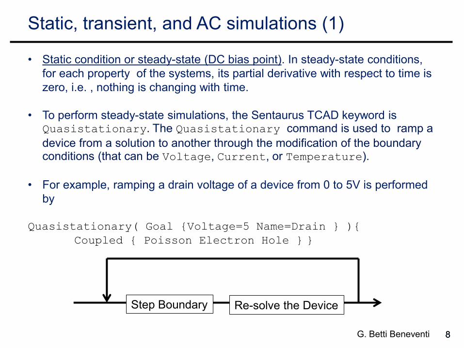
• For example, ramping a drain voltage of a device from 0 to 5V is performed
by
Quasistationary( Goal {Voltage=5 Name=Drain } ){
Coupled { Poisson Electron Hole } }
Step Boundary Re-solve the Device
9 9 G. Betti Beneventi
Static, transient, and AC simulations (2)
• Transient response. A transient response or natural response is the time-
varying response of a system to a change from equilibrium.
• In Sentaurus, the keyword that must be used to perform transient simulation is Transient. The command must start with a device that has already been
solved under stationary conditions. The simulation then proceeds by iterating
between incrementing time and re-solving the device.
• An example of performing a transient simulation is:
Transient( InitialTime = 0.0 FinalTime=1.0e-5 ){
Coupled { Poisson Electron Hole }
}
Increment time Re-solve the Device
10 10 G. Betti Beneventi
Static, transient, and AC simulations (3)
• Small signal AC analysis. Performing a small signal or AC analysis means
simulate the behavior of system when a relatively small harmonic signal is
superimposed to a steady-state condition or DC bias point.
• Small-signal modeling is a common analysis technique in electrical
engineering which is used to approximate the behavior of nonlinear devices
with linear equations. This linearization is formed about the DC bias point of
the device (that is, the voltage/current levels present when no AC signal is
applied), and can be accurate for small excursions about this point. • The keyword for AC analysis in Sentaurus Sdevice is ACCoupled.
Graphical, qualitative, illustration of steady-state, transient, and AC signals.
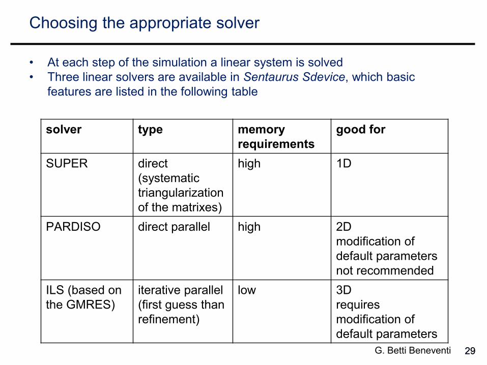
11 11 G. Betti Beneventi
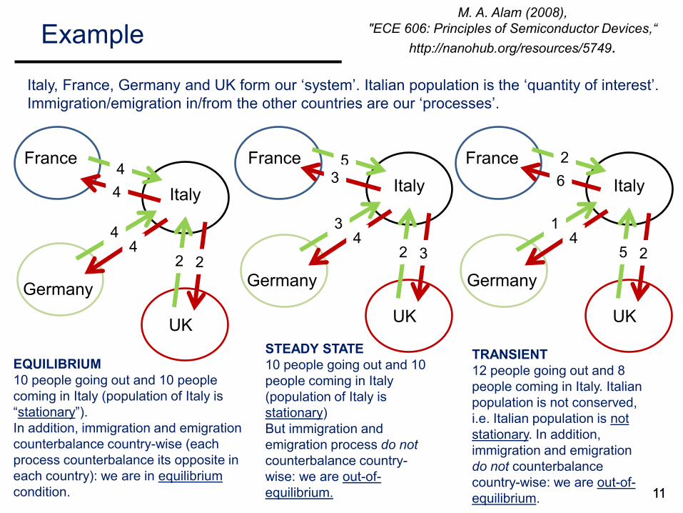
Example M. A. Alam (2008),
"ECE 606: Principles of Semiconductor Devices,“
http://nanohub.org/resources/5749.
EQUILIBRIUM
10 people going out and 10 people
coming in Italy (population of Italy is
“stationary”).
In addition, immigration and emigration
counterbalance country-wise (each
process counterbalance its opposite in
each country): we are in equilibrium
condition.
Italy, France, Germany and UK form our ‘system’. Italian population is the ‘quantity of interest’.
Immigration/emigration in/from the other countries are our ‘processes’.
TRANSIENT
12 people going out and 8
people coming in Italy. Italian
population is not conserved,
i.e. Italian population is not
stationary. In addition,
immigration and emigration
do not counterbalance
country-wise: we are out-of-
equilibrium.
STEADY STATE
10 people going out and 10
people coming in Italy
(population of Italy is
stationary)
But immigration and
emigration process do not
counterbalance country-
wise: we are out-of-
equilibrium.
Italy
France
Germany
UK
4
4
4 4
2 2
Italy
France
Germany
UK
5 3
3 4
3 2
Italy
France
Germany
UK
2
6
1 4
2 5
12 12 G. Betti Beneventi
Outline
• Introduction
• Definition of equilibrium and out-of-equilibrium
• Static, Transient and AC simulations
Simplify the simulation domain
• Numerical methods from a TCAD user
perspective
• Meshing
• Numerical methods
• Synopsys Sentaurus TCAD Solvers
13 13 G. Betti Beneventi
Simulation on 1D, 2D and 3D domains (1)
• Reality is always 3D. However, some problems can be thought (approximated) as they
would occur in less than 3D. This can be done when there is invariance of the problem
on some directions. In other words, a dimension can be suppressed from the simulation
if the physical internal properties of the simulated device would not change if the
dimension itself would be made infinite. To make such approximations (not always easy
to see!), an a-priori knowledge of the problem is needed.
Possible to think about a 2D equivalent (on
the yz plane) of what happens in the
transistor channel. That is the device features
can be thought to be invariant in the x
direction (within the channel). The larger the
L the better the 2D approximation.
Standard planar MOSFET FinFET
L very thin and raised
source and drain.
Intrinsically a 3D device,
very difficult to simplify
into a 2D equivalent!
2D
L L x
y
z
Example
14 14 G. Betti Beneventi
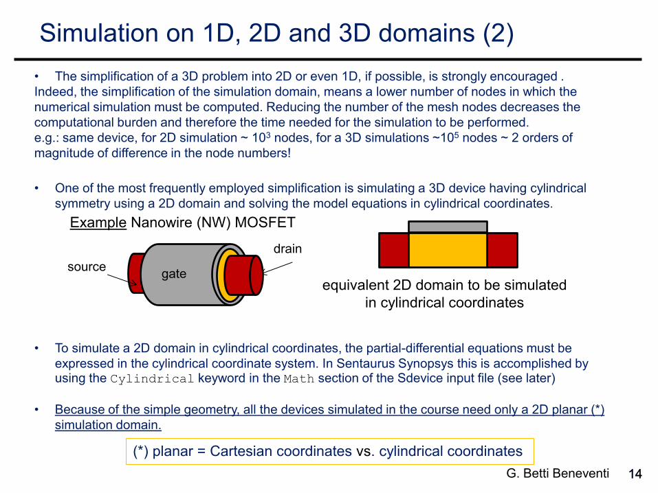
Simulation on 1D, 2D and 3D domains (2)
• The simplification of a 3D problem into 2D or even 1D, if possible, is strongly encouraged .
Indeed, the simplification of the simulation domain, means a lower number of nodes in which the
numerical simulation must be computed. Reducing the number of the mesh nodes decreases the
computational burden and therefore the time needed for the simulation to be performed.
e.g.: same device, for 2D simulation ~ 103 nodes, for a 3D simulations ~105 nodes ~ 2 orders of
magnitude of difference in the node numbers!
• One of the most frequently employed simplification is simulating a 3D device having cylindrical
symmetry using a 2D domain and solving the model equations in cylindrical coordinates.
• To simulate a 2D domain in cylindrical coordinates, the partial-differential equations must be
expressed in the cylindrical coordinate system. In Sentaurus Synopsys this is accomplished by using the Cylindrical keyword in the Math section of the Sdevice input file (see later)
• Because of the simple geometry, all the devices simulated in the course need only a 2D planar (*)
simulation domain.
equivalent 2D domain to be simulated
in cylindrical coordinates
(*) planar = Cartesian coordinates vs. cylindrical coordinates
Example Nanowire (NW) MOSFET
source
drain
gate
15 15 G. Betti Beneventi
Outline
• Introduction
• Definition of equilibrium and out-of-equilibrium
• Static, Transient and AC simulations
• Simplify the simulation domain
Numerical methods from a TCAD user
perspective
• Meshing
• Numerical methods
• Synopsys Sentaurus TCAD Solvers
16 16 G. Betti Beneventi
Scope
• In this tutorial we discuss the basic features of the numerical method
used in TCAD Sentaurus Devices from a TCAD user perspective.
The purpose of this tutorial is not describing into details the
numerical methods implemented in the software, but discussing their
general features, in order for the user to understand which numerical
methods is most useful to be employed for a given problem and to
cope with possible convergence issues.
• In general, in an iterative solution method, we start with a guess for
the solution (often the zero vector) and then we successively renew
this guess, getting closer to the solution at each stage. The
iterations continue until the solution converges to a desired accuracy
xi –xi-1 < e, where x is the solution vector, that is the vector of the
values of the problem unknowns, i is the index counting the iteration
number, and e is the vector which defines the needed accuracy.
17 17 G. Betti Beneventi
Outline
• Introduction
• Definition of equilibrium and out-of-equilibrium
• Static, Transient and AC simulations
• Simplify the simulation domain
• Numerical methods from a TCAD user
perspective
Meshing
• Numerical methods
• Synopsys Sentaurus TCAD Solvers
18 18 G. Betti Beneventi
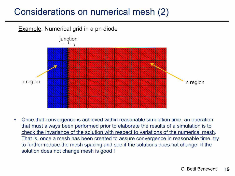
Considerations on numerical mesh (1)
• Define and effectively optimize numerical meshes in which the problem can be solved
assuring convergence and, at the same time, reasonable simulation times, is a
challenge. However, some general rules can be applied:
• The grid spacing must be sufficiently dense so that all the relevant features of the
geometry (e.g. doping) are accurately represented.
• Points must be allocated to accurately approximate the physical quantities of


![Free Open Source Mesh Healing for TCAD Device · PDF fileple, Synopsys Sentaurus TCAD provides a structure editor for modeling device geometries [3]. ... Free Open Source Mesh Healing](https://static.documents.pub/doc/80x56/5a9cd7257f8b9aba4a8e743e/free-open-source-mesh-healing-for-tcad-device-synopsys-sentaurus-tcad-provides-a.jpg)
![TCAD for reliability - Semantic Scholar · PDF fileTCAD for reliability ... opsys Sentaurus TCAD [1], are well established for modeling semi-conductor fabrication process, and device](https://static.documents.pub/doc/80x56/5a9cd7257f8b9aba4a8e7433/tcad-for-reliability-semantic-scholar-for-reliability-opsys-sentaurus-tcad.jpg)


![VARI: CERVENKAetal.: TCAD SIMULATION OF … · The 143 process simulations have been set up in Sentaurus Workbench (SWB) of the TCAD simulation package of SYN-OPSYS [3].](https://static.documents.pub/doc/80x56/5b5687f07f8b9a022e8c9fb2/vari-cervenkaetal-tcad-simulation-of-the-143-process-simulations-have-been.jpg)