Testing of Fiber-Optics for Use in CLAS12 PCAL Detector Aaron Kearns Advisor: Dr. Jeffrey Nelson Abstract This experiment intends to test fibers for use in the CLAS12 PCAL detector. This detector uses a series of plastic scintillators along with wavelength-shifting fibers in order to detect electron/positron pairs produced by the decay of neutral pions. In setting up the testing conditions for the experiment, a custom connection between these fibers and a photomultiplier tube was created, and absolute light yield was improved by cutting the fiber tips with a heated razor. This has given us a consistent set of control fiber measurements that can be used to verify the quality of additional fibers for use in the detector as they become available to test.
Transcript
Testing of Fiber-Optics for Use in CLAS12 PCAL Detector
Aaron Kearns
Advisor: Dr. Jeffrey Nelson
Abstract
This experiment intends to test fibers for use in the CLAS12 PCAL detector. This detector
uses a series of plastic scintillators along with wavelength-shifting fibers in order to
detect electron/positron pairs produced by the decay of neutral pions. In setting up the
testing conditions for the experiment, a custom connection between these fibers and a
photomultiplier tube was created, and absolute light yield was improved by cutting the
fiber tips with a heated razor. This has given us a consistent set of control fiber
measurements that can be used to verify the quality of additional fibers for use in the
detector as they become available to test.
Overview
The CLAS detector, short for CEBAF Large Acceptance Spectrometer, is an apparatus used in
experiments in Hall B in the Thomas Jefferson National Accelerator Facility (JLAB). This is a fixed-target
experiment, in that an electron beam is fired at stationary target nuclei. When the electrons hit these
nuclei, various particles come out, and the original electrons energy is shifted. The goal of CLAS is to
determine what sorts of particles come out of the detector; there are multiple components which are
designed to detect some of the produced particles.
One such detector is the pre-shower calorimeter (PCAL), used to detect neutral pion (π°) decay.
The π° is unstable and decays quickly into a pair of photons (γ), with energy E/2 compared to the π°.
These γ then can decay into an electron-positron pair (e+/e-), each with E/2 compared to the γ (E/4
overall). The e+/e- then may interact with a nucleus, and as long as they are above a certain energy, they
will cause stimulated emission of another γ as well as the original particle, again with each getting E/2
compared to the original e+/e-. This reaction can continue until the electron or positron is below a
critical energy, at which point it is simply absorbed and not re-emitted. [Longair] The goal of PCAL is to
detect the first pair of charged particles produced by this interaction.
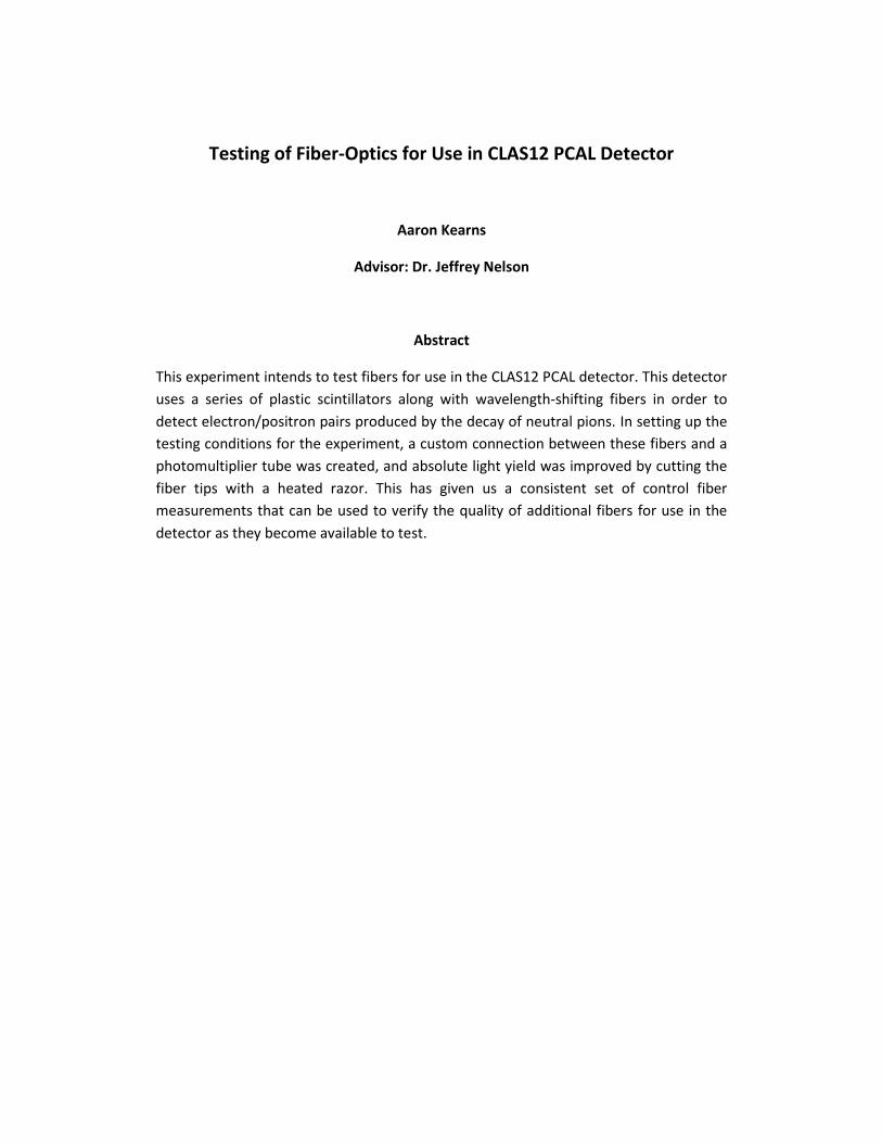
PCAL detects particles through the use of plastic scintillators and fiber-optics. The scintillator is a
length of polystyrene that has a reflective coat. It allows high-energy particles in and then traps them.
Interactions with the nuclei in the scintillator produce e+/e- pairs, as mentioned above. The plastic is
doped with two organic molecules, PPO and POPOP, which emit photons when hit by ionizing radiation
such as these charged particles. These photons are carried along an optical fiber, which leads to a
photomultiplier tube, producing an electrical signal proportional to the number of photons produced by
the scintillator and thus the number of e+/e- interactions.
Figure 1 Example of scintillator with green fibers [Kantner]
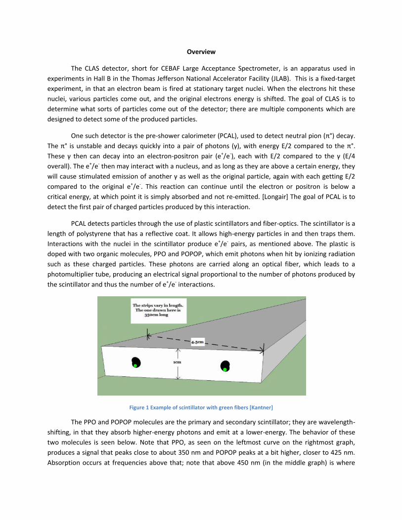
The PPO and POPOP molecules are the primary and secondary scintillator; they are wavelength-
shifting, in that they absorb higher-energy photons and emit at a lower-energy. The behavior of these
two molecules is seen below. Note that PPO, as seen on the leftmost curve on the rightmost graph,
produces a signal that peaks close to about 350 nm and POPOP peaks at a bit higher, closer to 425 nm.
Absorption occurs at frequencies above that; note that above 450 nm (in the middle graph) is where
most of the absorption in POPOP begins; the absorption length is the distance where the proportion of
electrons not absorbed by the scintillator is 1/e.
Figure 2 Graph of PPO and POPOP absorption and emission levels. [Pahlka]
Once the photon signal has been produced by one of the scintillators, it needs to be carried to a
photomultiplier tube; again, this is done using an optical fiber. An optical fiber transmits photons along
its length by total internal reflection. This occurs when the outer surface of a material has a lower
refraction index than the rest of the material; if the angle of the light entering the fiber is past a critical
angle with the normal, the light becomes effectively trapped in the scintillator, reflecting off the inside
of the surface of the fiber, carried toward a counter. In the case of the fibers used in this experiment,
the outer cladding has an index of 1.4 and the inner surface has an index of 1.6 [Nelson], and the critical
angle is calculated as follows:
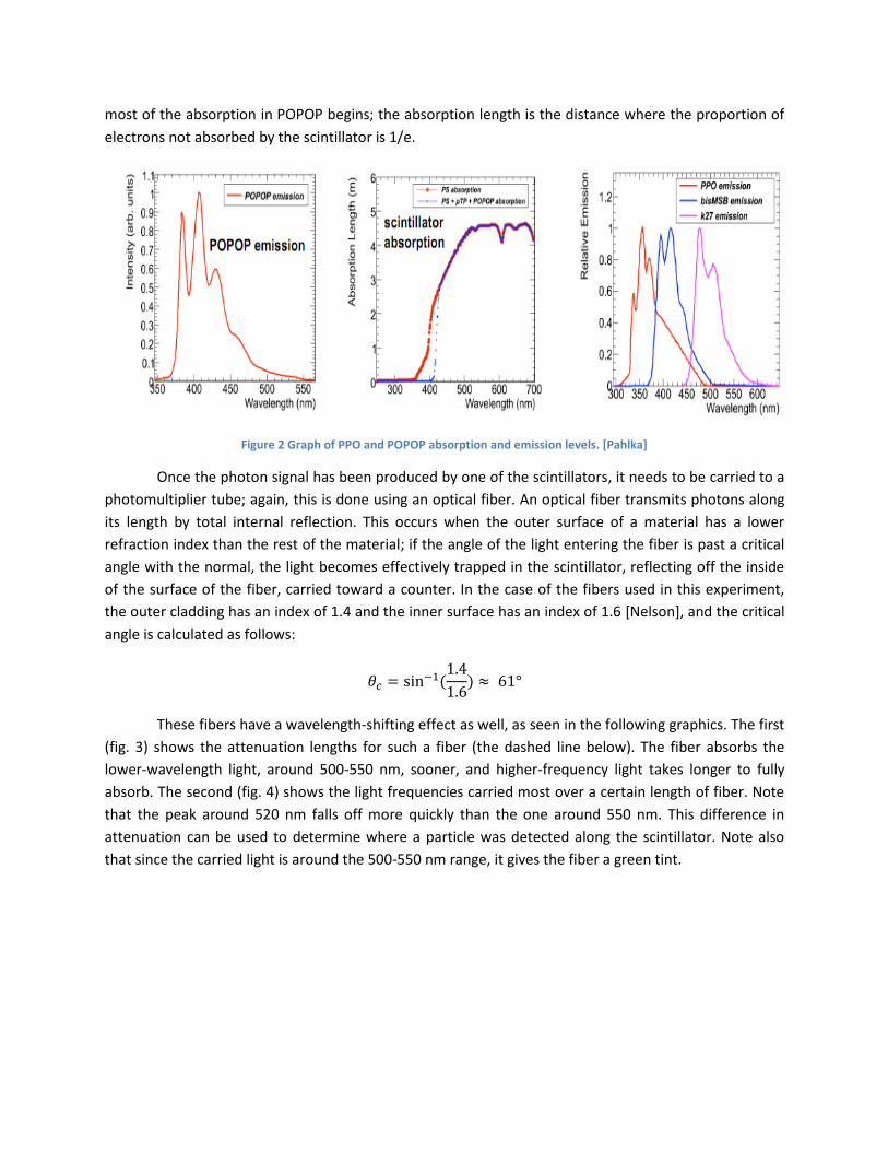
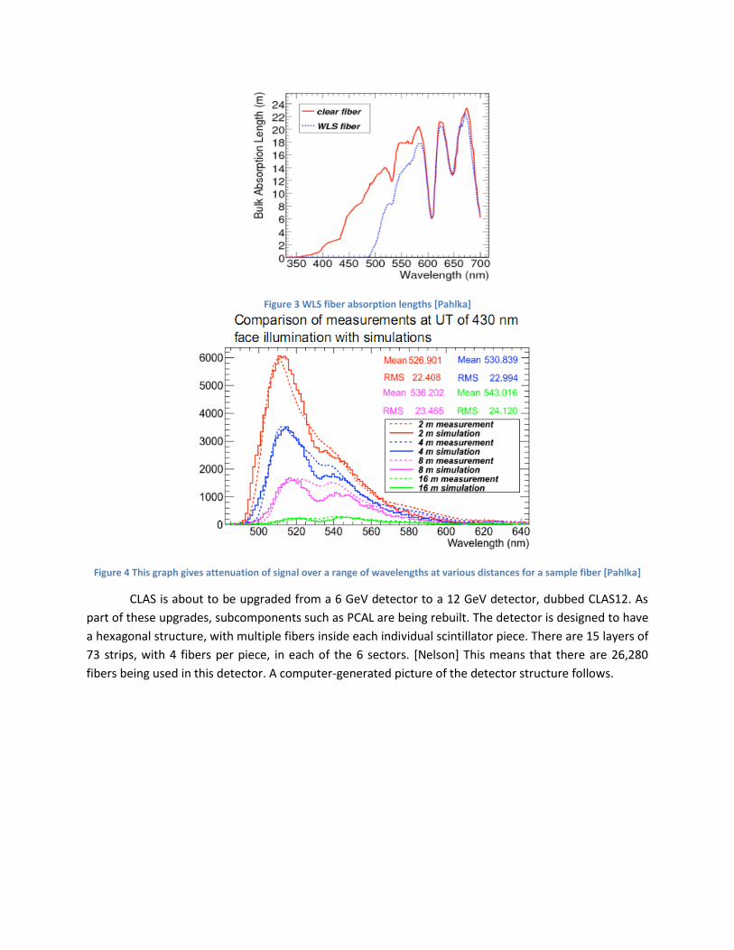
These fibers have a wavelength-shifting effect as well, as seen in the following graphics. The first
(fig. 3) shows the attenuation lengths for such a fiber (the dashed line below). The fiber absorbs the
lower-wavelength light, around 500-550 nm, sooner, and higher-frequency light takes longer to fully
absorb. The second (fig. 4) shows the light frequencies carried most over a certain length of fiber. Note
that the peak around 520 nm falls off more quickly than the one around 550 nm. This difference in
attenuation can be used to determine where a particle was detected along the scintillator. Note also
that since the carried light is around the 500-550 nm range, it gives the fiber a green tint.
Figure 3 WLS fiber absorption lengths [Pahlka]
Figure 4 This graph gives attenuation of signal over a range of wavelengths at various distances for a sample fiber [Pahlka]
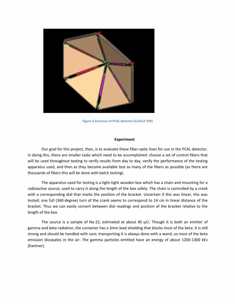
CLAS is about to be upgraded from a 6 GeV detector to a 12 GeV detector, dubbed CLAS12. As
part of these upgrades, subcomponents such as PCAL are being rebuilt. The detector is designed to have
a hexagonal structure, with multiple fibers inside each individual scintillator piece. There are 15 layers of
73 strips, with 4 fibers per piece, in each of the 6 sectors. [Nelson] This means that there are 26,280
fibers being used in this detector. A computer-generated picture of the detector structure follows.
Figure 5 Structure of PCAL detector (CLAS12 TDR)
Experiment
Our goal for this project, then, is to evaluate these fiber-optic lines for use in the PCAL detector.
In doing this, there are smaller tasks which need to be accomplished: choose a set of control fibers that
will be used throughout testing to verify results from day to day, verify the performance of the testing
apparatus used, and then as they become available test as many of the fibers as possible (as there are
thousands of fibers this will be done with batch testing).
The apparatus used for testing is a light-tight wooden box which has a chain and mounting for a
radioactive source, used to carry it along the length of the box safely. The chain is controlled by a crank
with a corresponding dial that marks the position of the bracket. Uncertain if this was linear, this was
tested; one full (360-degree) turn of the crank seems to correspond to 14 cm in linear distance of the
bracket. Thus we can easily convert between dial readings and position of the bracket relative to the
length of the box.
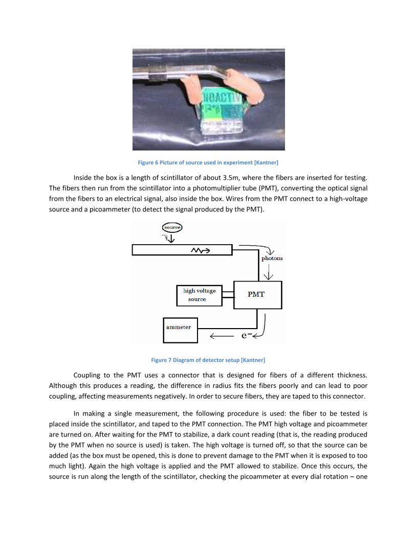
The source is a sample of Na-22, estimated at about 40 µCi. Though it is both an emitter of
gamma and beta radiation, the container has a 3mm lead shielding that blocks most of the beta. It is still
strong and should be handled with care; transporting it is always done with a wand, so most of the beta
emission dissipates in the air. The gamma particles emitted have an energy of about 1200-1300 kEv
[Kantner].
Figure 6 Picture of source used in experiment [Kantner]
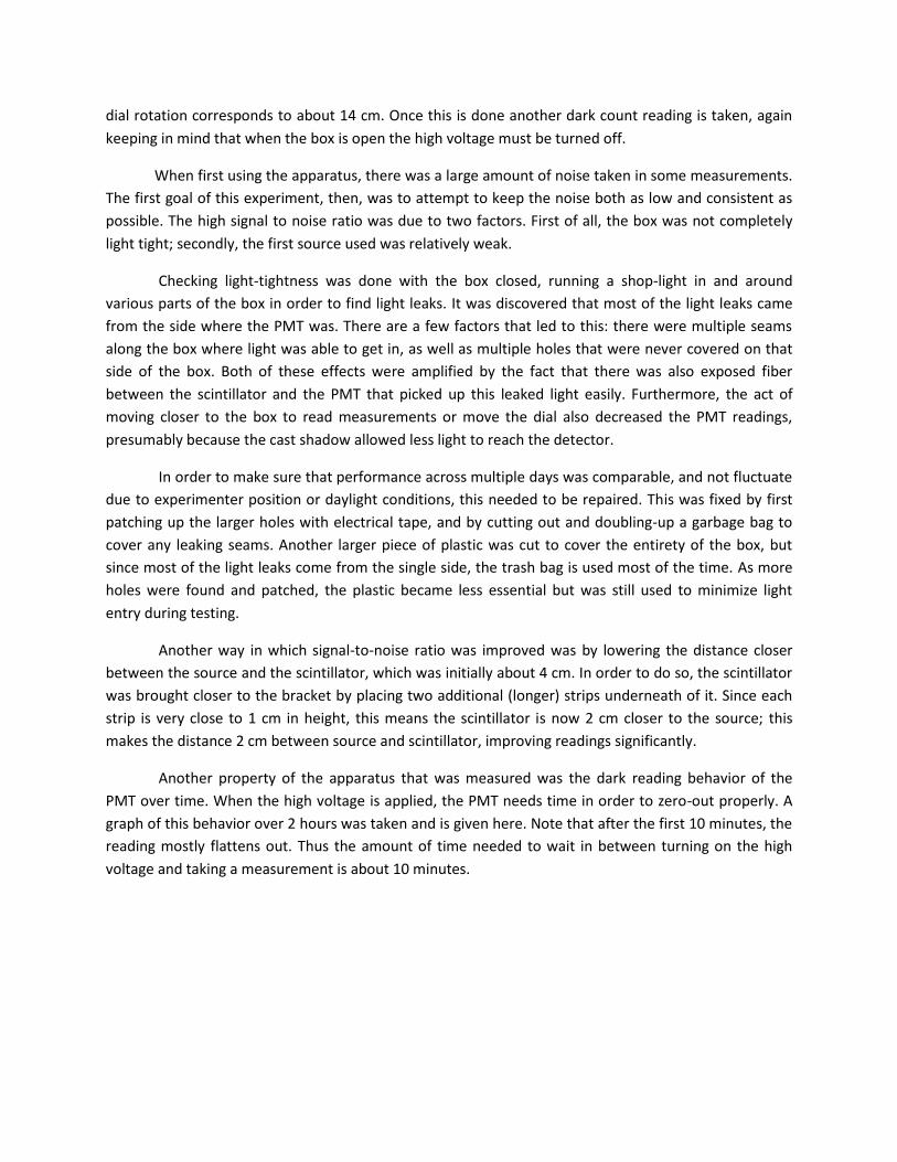
Inside the box is a length of scintillator of about 3.5m, where the fibers are inserted for testing.
The fibers then run from the scintillator into a photomultiplier tube (PMT), converting the optical signal
from the fibers to an electrical signal, also inside the box. Wires from the PMT connect to a high-voltage
source and a picoammeter (to detect the signal produced by the PMT).
Figure 7 Diagram of detector setup [Kantner]
Coupling to the PMT uses a connector that is designed for fibers of a different thickness.
Although this produces a reading, the difference in radius fits the fibers poorly and can lead to poor
coupling, affecting measurements negatively. In order to secure fibers, they are taped to this connector.
In making a single measurement, the following procedure is used: the fiber to be tested is
placed inside the scintillator, and taped to the PMT connection. The PMT high voltage and picoammeter
are turned on. After waiting for the PMT to stabilize, a dark count reading (that is, the reading produced
by the PMT when no source is used) is taken. The high voltage is turned off, so that the source can be
added (as the box must be opened, this is done to prevent damage to the PMT when it is exposed to too
much light). Again the high voltage is applied and the PMT allowed to stabilize. Once this occurs, the
source is run along the length of the scintillator, checking the picoammeter at every dial rotation – one
dial rotation corresponds to about 14 cm. Once this is done another dark count reading is taken, again
keeping in mind that when the box is open the high voltage must be turned off.
When first using the apparatus, there was a large amount of noise taken in some measurements.
The first goal of this experiment, then, was to attempt to keep the noise both as low and consistent as
possible. The high signal to noise ratio was due to two factors. First of all, the box was not completely
light tight; secondly, the first source used was relatively weak.
Checking light-tightness was done with the box closed, running a shop-light in and around
various parts of the box in order to find light leaks. It was discovered that most of the light leaks came
from the side where the PMT was. There are a few factors that led to this: there were multiple seams
along the box where light was able to get in, as well as multiple holes that were never covered on that
side of the box. Both of these effects were amplified by the fact that there was also exposed fiber
between the scintillator and the PMT that picked up this leaked light easily. Furthermore, the act of
moving closer to the box to read measurements or move the dial also decreased the PMT readings,
presumably because the cast shadow allowed less light to reach the detector.
In order to make sure that performance across multiple days was comparable, and not fluctuate
due to experimenter position or daylight conditions, this needed to be repaired. This was fixed by first
patching up the larger holes with electrical tape, and by cutting out and doubling-up a garbage bag to
cover any leaking seams. Another larger piece of plastic was cut to cover the entirety of the box, but
since most of the light leaks come from the single side, the trash bag is used most of the time. As more
holes were found and patched, the plastic became less essential but was still used to minimize light
entry during testing.
Another way in which signal-to-noise ratio was improved was by lowering the distance closer
between the source and the scintillator, which was initially about 4 cm. In order to do so, the scintillator
was brought closer to the bracket by placing two additional (longer) strips underneath of it. Since each
strip is very close to 1 cm in height, this means the scintillator is now 2 cm closer to the source; this
makes the distance 2 cm between source and scintillator, improving readings significantly.
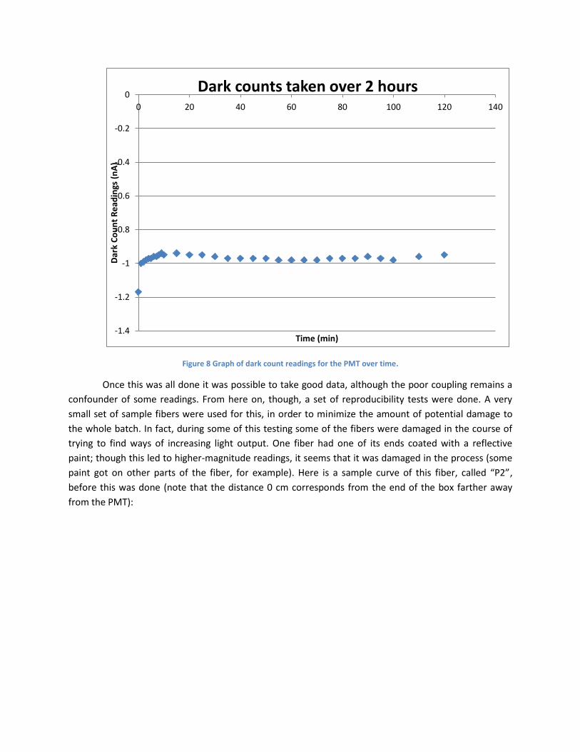
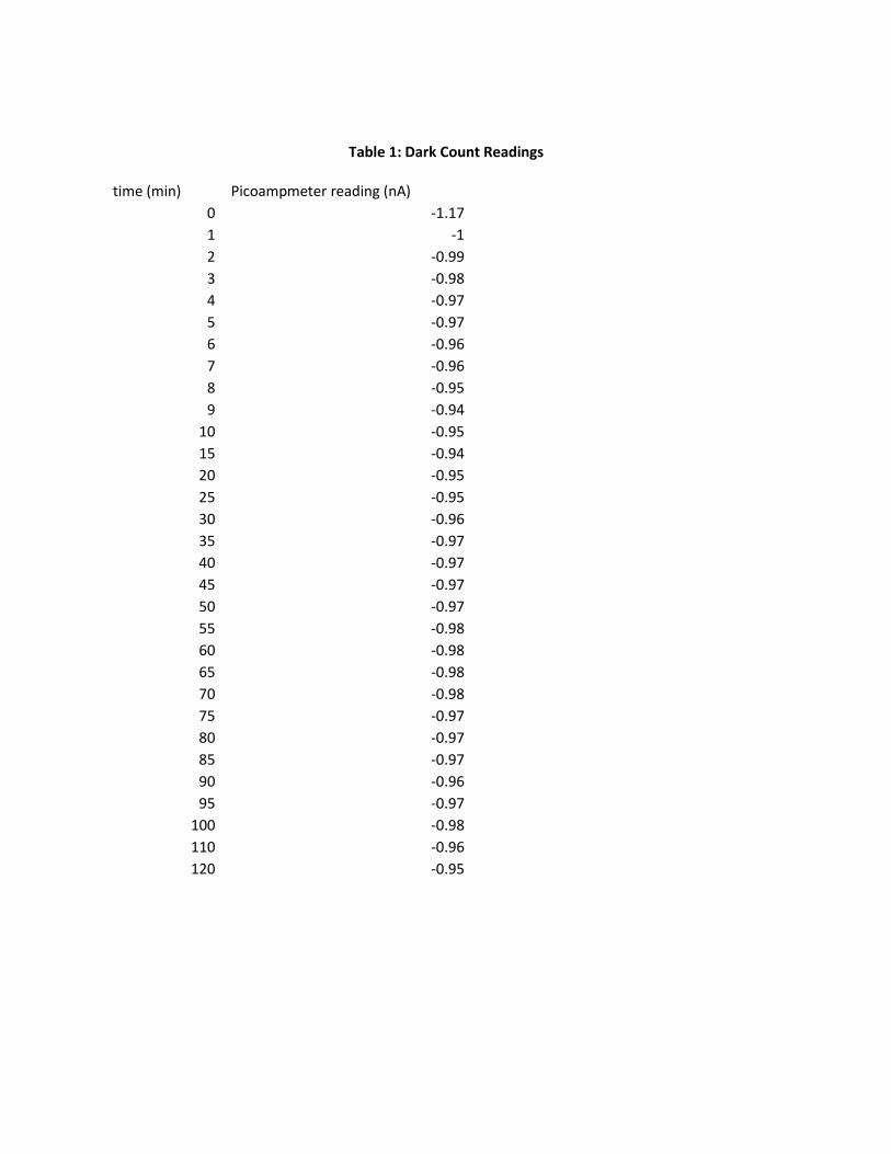
Another property of the apparatus that was measured was the dark reading behavior of the
PMT over time. When the high voltage is applied, the PMT needs time in order to zero-out properly. A
graph of this behavior over 2 hours was taken and is given here. Note that after the first 10 minutes, the
reading mostly flattens out. Thus the amount of time needed to wait in between turning on the high
voltage and taking a measurement is about 10 minutes.
Figure 8 Graph of dark count readings for the PMT over time.
Once this was all done it was possible to take good data, although the poor coupling remains a
confounder of some readings. From here on, though, a set of reproducibility tests were done. A very
small set of sample fibers were used for this, in order to minimize the amount of potential damage to
the whole batch. In fact, during some of this testing some of the fibers were damaged in the course of
trying to find ways of increasing light output. One fiber had one of its ends coated with a reflective
paint; though this led to higher-magnitude readings, it seems that it was damaged in the process (some
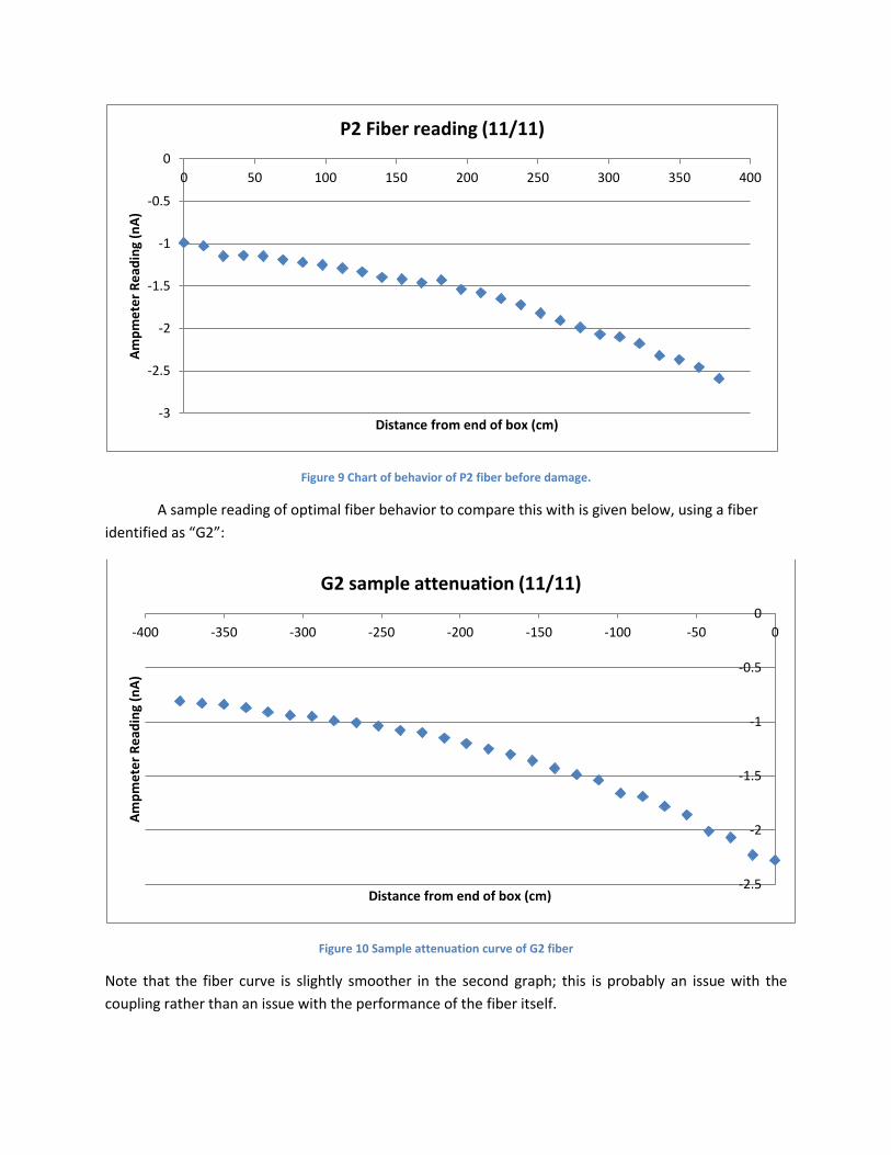
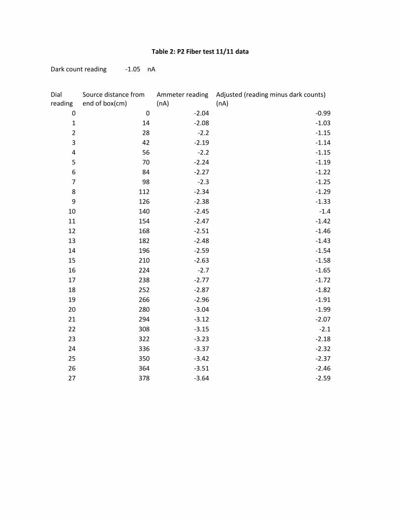
paint got on other parts of the fiber, for example). Here is a sample curve of this fiber, called “P2”,
before this was done (note that the distance 0 cm corresponds from the end of the box farther away
from the PMT):
-1.4
-1.2
-1
-0.8
-0.6
-0.4
-0.2
0
0 20 40 60 80 100 120 140D
ark
Co
un
t R
ead
ings
(n
A)
Time (min)
Dark counts taken over 2 hours
Figure 9 Chart of behavior of P2 fiber before damage.
A sample reading of optimal fiber behavior to compare this with is given below, using a fiber
identified as “G2”:
Figure 10 Sample attenuation curve of G2 fiber
Note that the fiber curve is slightly smoother in the second graph; this is probably an issue with the
coupling rather than an issue with the performance of the fiber itself.
-3
-2.5
-2
-1.5
-1
-0.5
0
0 50 100 150 200 250 300 350 400
Am
pm
ete
r R
ead
ing
(nA
)
Distance from end of box (cm)
P2 Fiber reading (11/11)
-2.5
-2
-1.5
-1
-0.5
0
-400 -350 -300 -250 -200 -150 -100 -50 0
Am
pm
ete
r R
ead
ing
(nA
)
Distance from end of box (cm)
G2 sample attenuation (11/11)
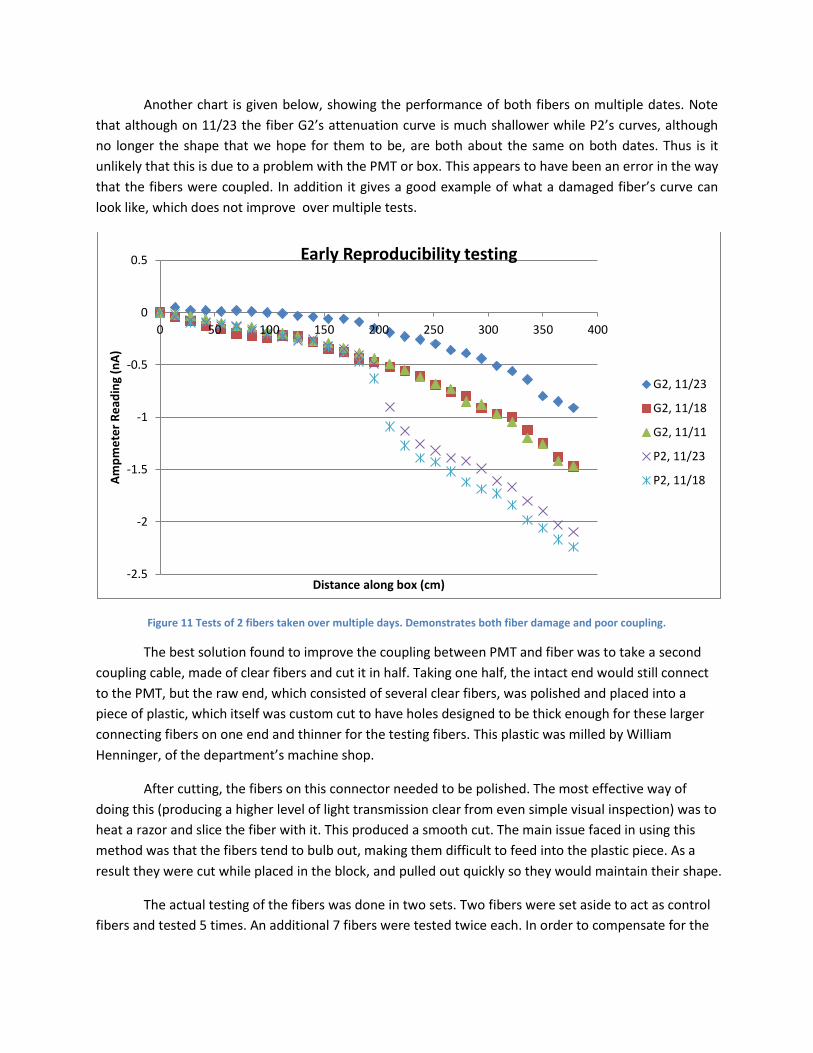
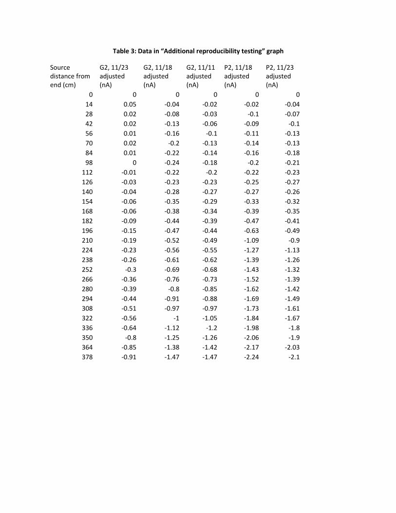
Another chart is given below, showing the performance of both fibers on multiple dates. Note
that although on 11/23 the fiber G2’s attenuation curve is much shallower while P2’s curves, although
no longer the shape that we hope for them to be, are both about the same on both dates. Thus is it
unlikely that this is due to a problem with the PMT or box. This appears to have been an error in the way
that the fibers were coupled. In addition it gives a good example of what a damaged fiber’s curve can
look like, which does not improve over multiple tests.
Figure 11 Tests of 2 fibers taken over multiple days. Demonstrates both fiber damage and poor coupling.
The best solution found to improve the coupling between PMT and fiber was to take a second
coupling cable, made of clear fibers and cut it in half. Taking one half, the intact end would still connect
to the PMT, but the raw end, which consisted of several clear fibers, was polished and placed into a
piece of plastic, which itself was custom cut to have holes designed to be thick enough for these larger
connecting fibers on one end and thinner for the testing fibers. This plastic was milled by William
Henninger, of the department’s machine shop.
After cutting, the fibers on this connector needed to be polished. The most effective way of
doing this (producing a higher level of light transmission clear from even simple visual inspection) was to
heat a razor and slice the fiber with it. This produced a smooth cut. The main issue faced in using this
method was that the fibers tend to bulb out, making them difficult to feed into the plastic piece. As a
result they were cut while placed in the block, and pulled out quickly so they would maintain their shape.
The actual testing of the fibers was done in two sets. Two fibers were set aside to act as control
fibers and tested 5 times. An additional 7 fibers were tested twice each. In order to compensate for the
-2.5
-2
-1.5
-1
-0.5
0
0.5
0 50 100 150 200 250 300 350 400
Am
pm
ete
r R
ead
ing
(nA
)
Distance along box (cm)
Early Reproducibility testing
G2, 11/23
G2, 11/18
G2, 11/11
P2, 11/23
P2, 11/18
PMT’s behavior over time during the taking of a single data set, one run was done moving down the
apparatus (toward the PMT) and the other was done moving in the opposite direction.
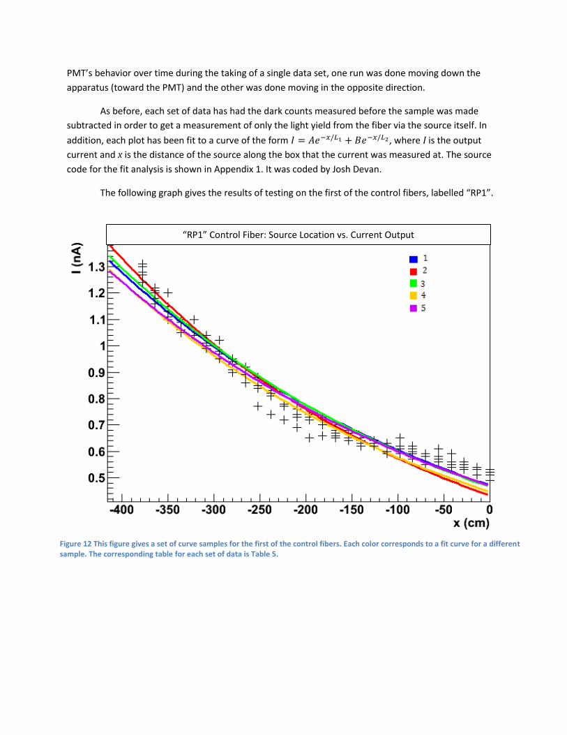
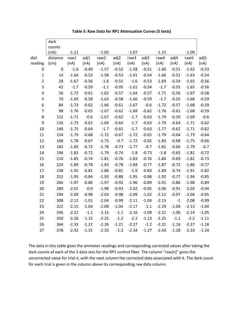
As before, each set of data has had the dark counts measured before the sample was made
subtracted in order to get a measurement of only the light yield from the fiber via the source itself. In
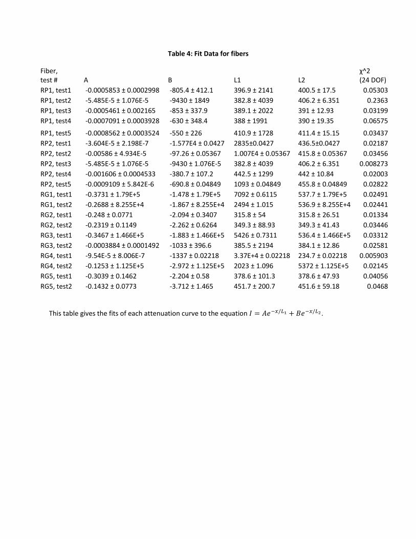
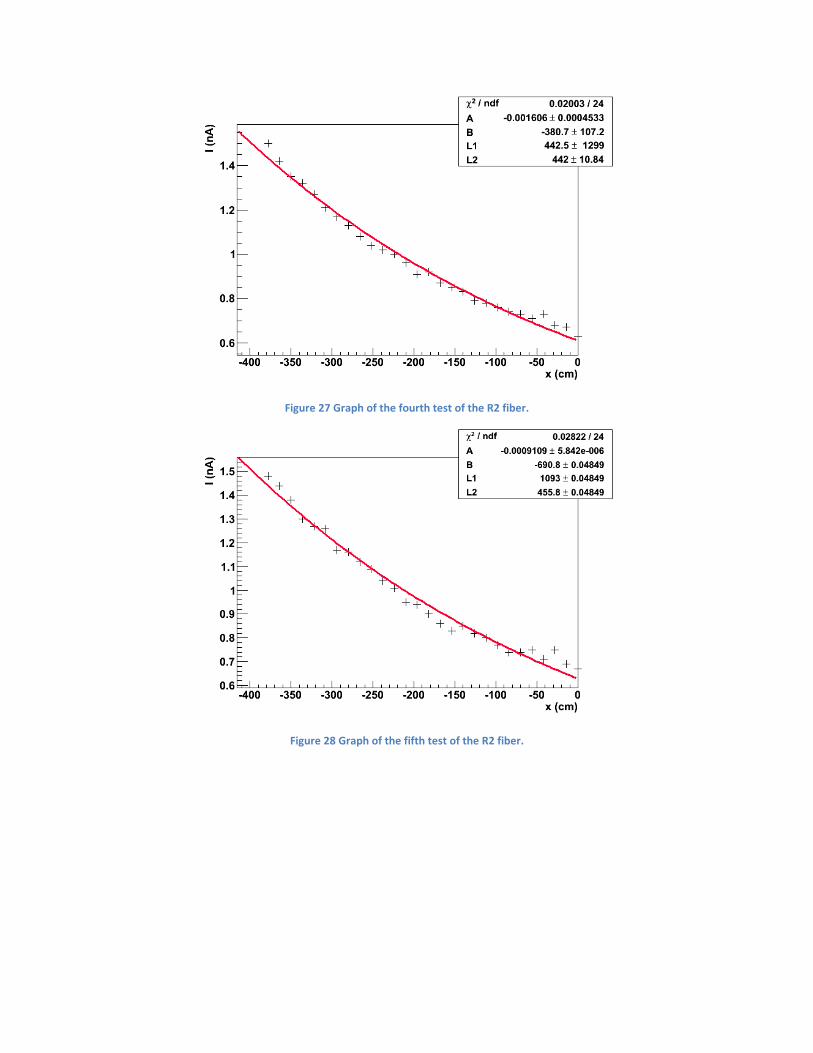
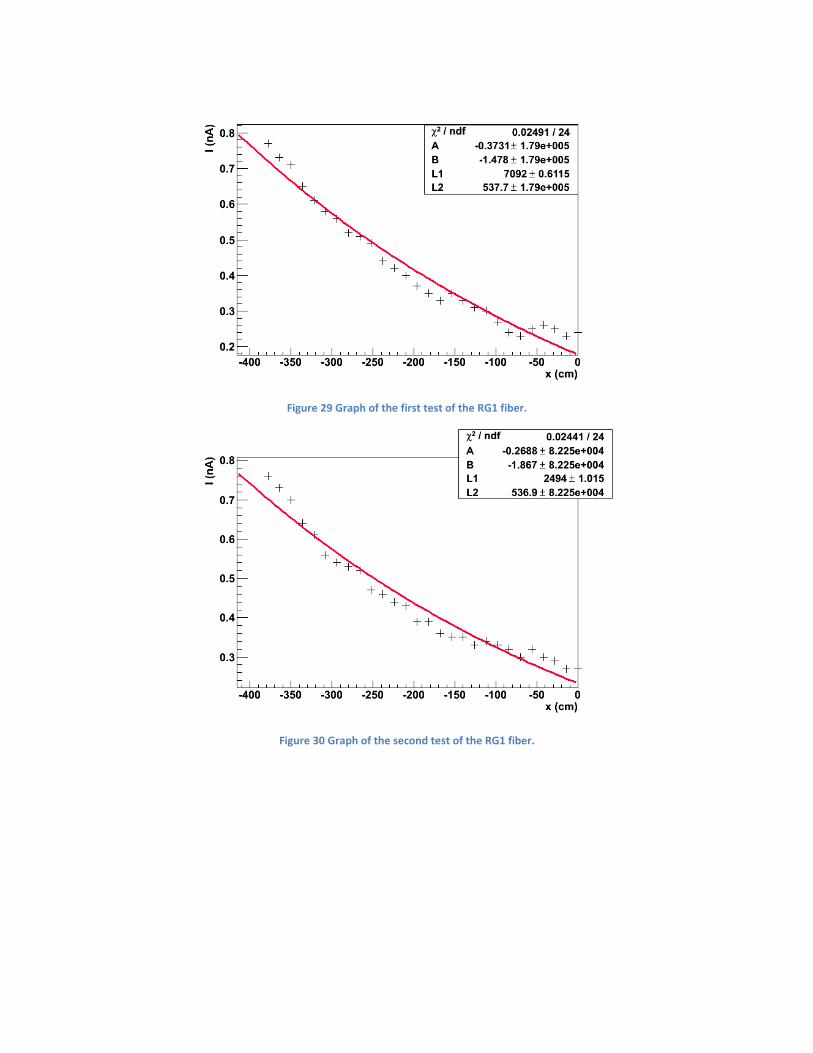
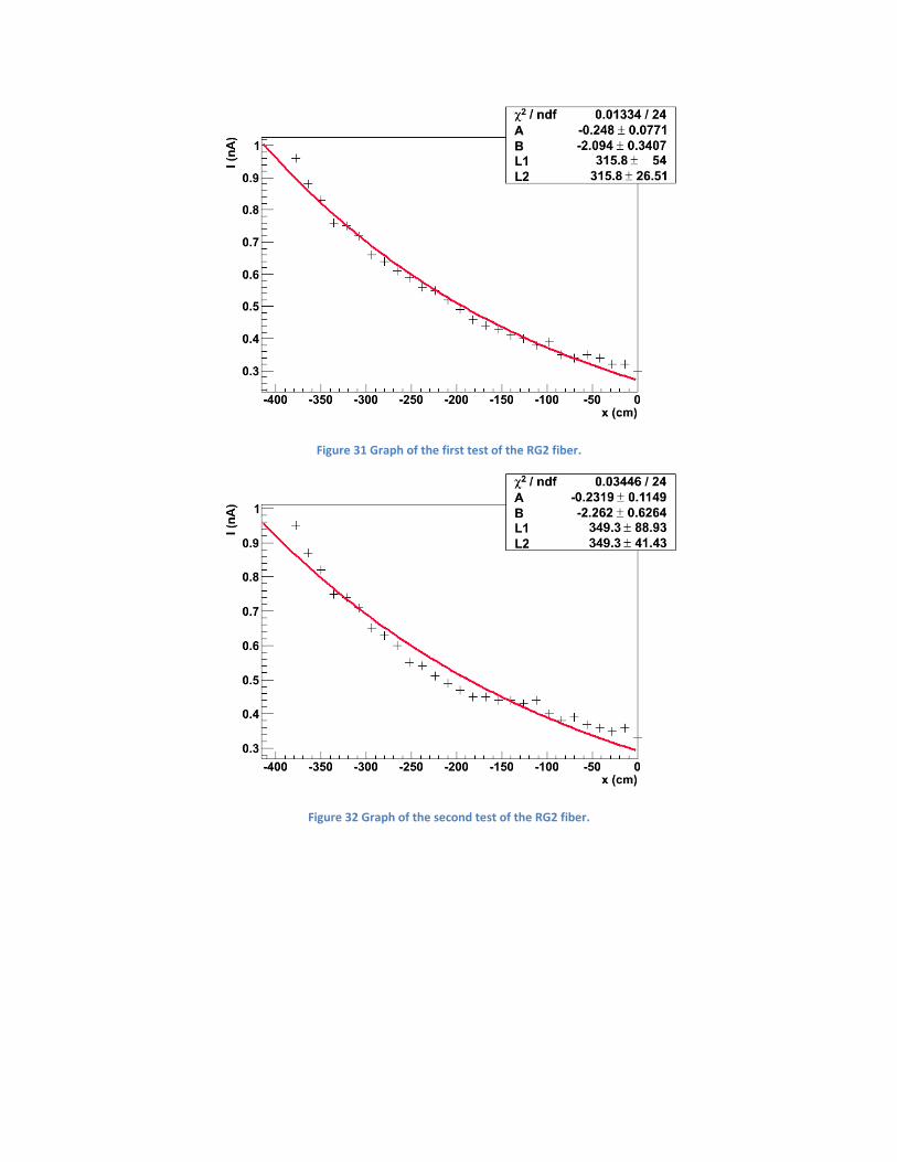
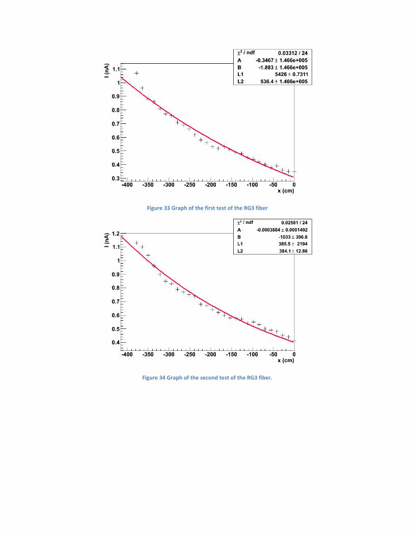
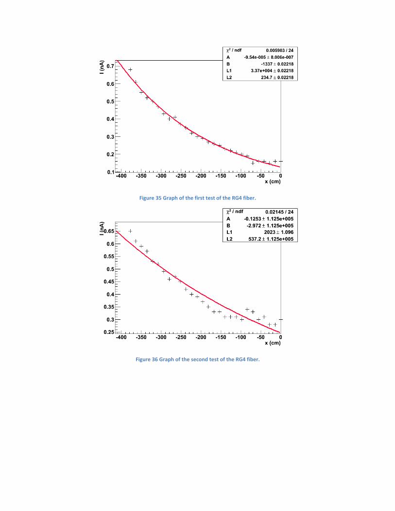
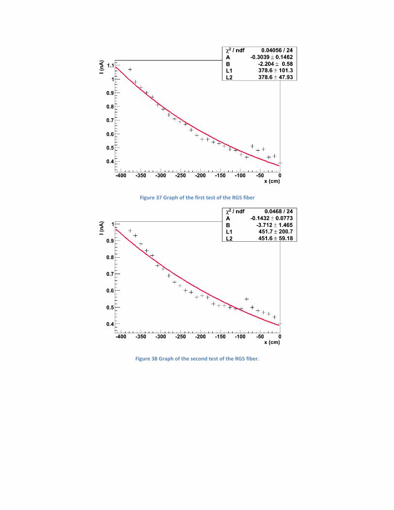
addition, each plot has been fit to a curve of the form , where I is the output
current and x is the distance of the source along the box that the current was measured at. The source
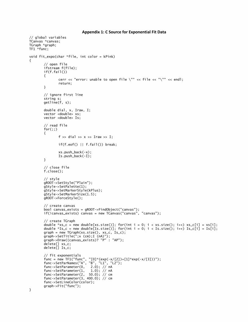
code for the fit analysis is shown in Appendix 1. It was coded by Josh Devan.
The following graph gives the results of testing on the first of the control fibers, labelled “RP1”.
Figure 12 This figure gives a set of curve samples for the first of the control fibers. Each color corresponds to a fit curve for a different sample. The corresponding table for each set of data is Table 5.
“RP1” Control Fiber: Source Location vs. Current Output
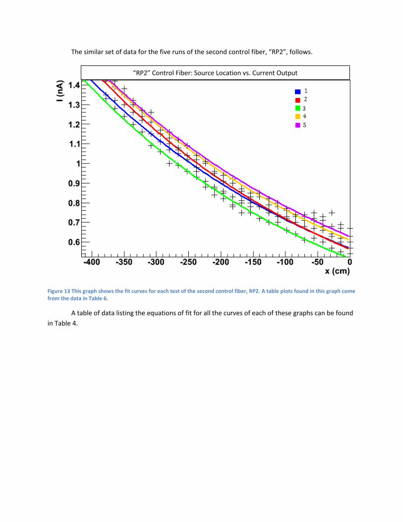
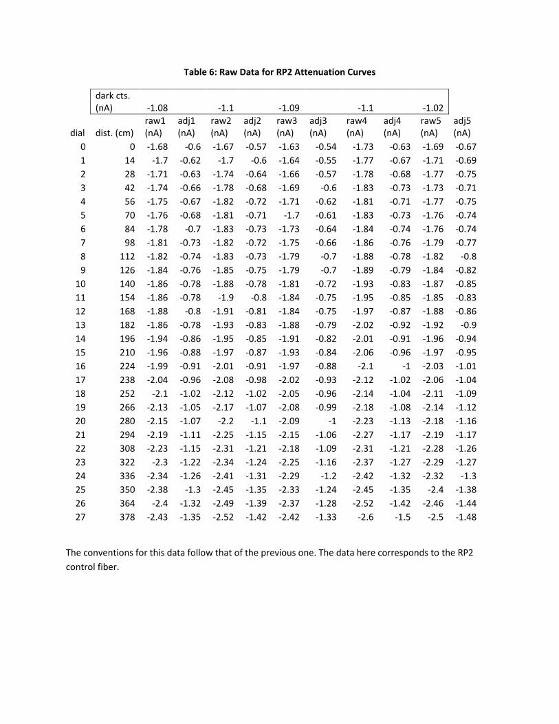
The similar set of data for the five runs of the second control fiber, “RP2”, follows.
Figure 13 This graph shows the fit curves for each test of the second control fiber, RP2. A table plots found in this graph come from the data in Table 6.
A table of data listing the equations of fit for all the curves of each of these graphs can be found
in Table 4.
“RP2” Control Fiber: Source Location vs. Current Output
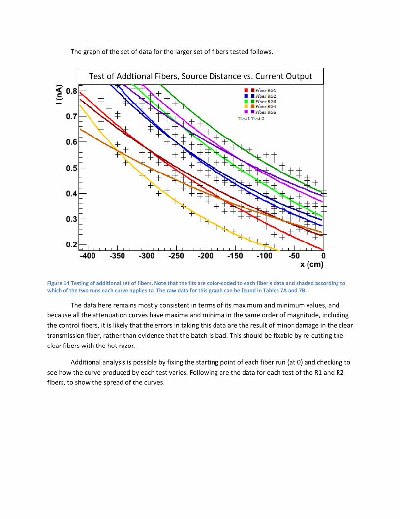
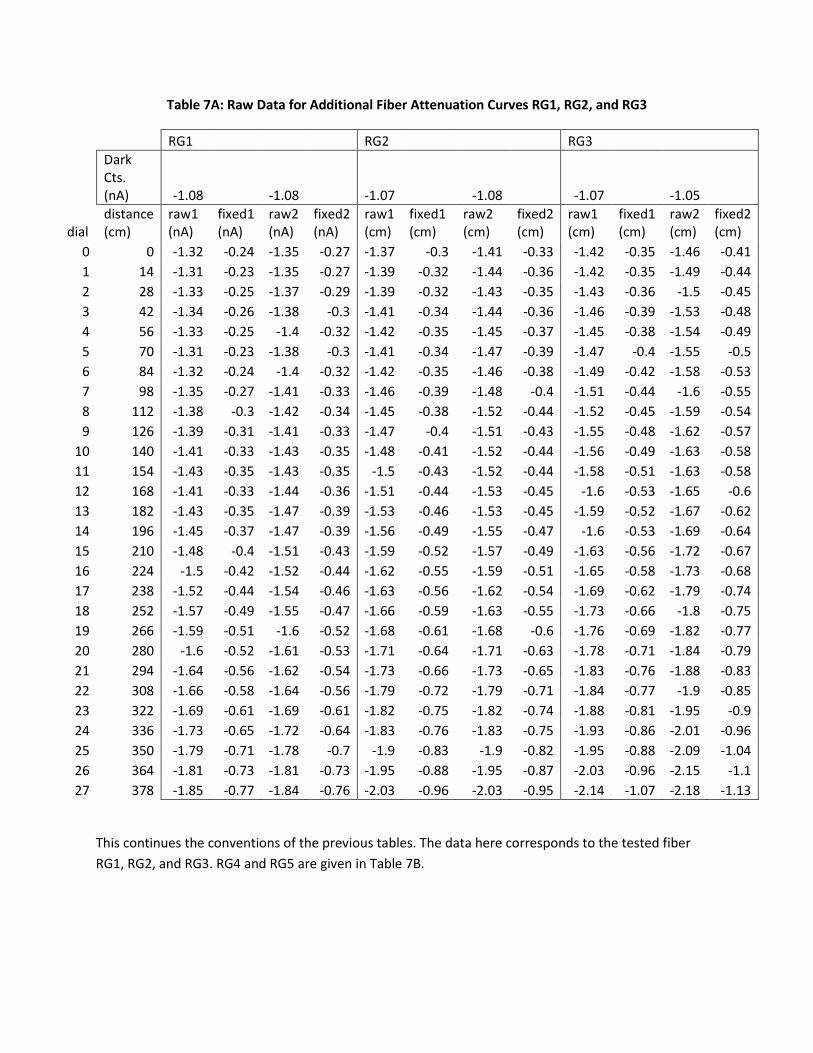
The graph of the set of data for the larger set of fibers tested follows.
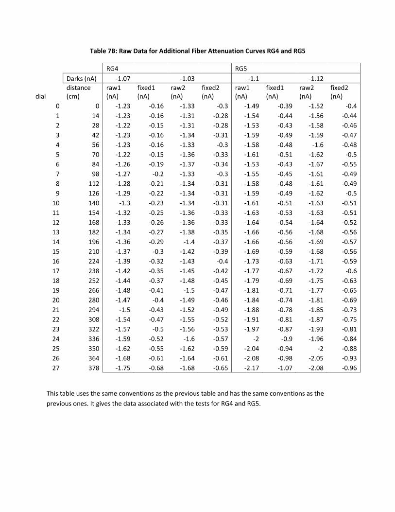
Figure 14 Testing of additional set of fibers. Note that the fits are color-coded to each fiber's data and shaded according to which of the two runs each curve applies to. The raw data for this graph can be found in Tables 7A and 7B.
The data here remains mostly consistent in terms of its maximum and minimum values, and
because all the attenuation curves have maxima and minima in the same order of magnitude, including
the control fibers, it is likely that the errors in taking this data are the result of minor damage in the clear
transmission fiber, rather than evidence that the batch is bad. This should be fixable by re-cutting the
clear fibers with the hot razor.
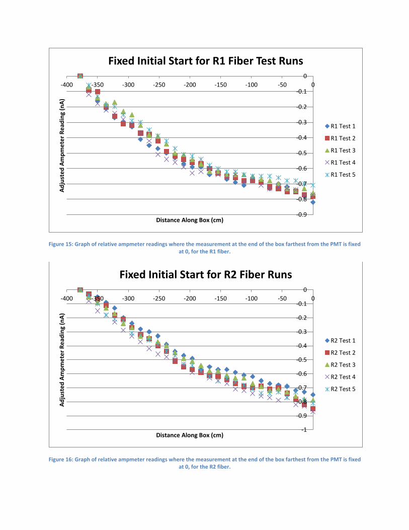
Additional analysis is possible by fixing the starting point of each fiber run (at 0) and checking to
see how the curve produced by each test varies. Following are the data for each test of the R1 and R2
fibers, to show the spread of the curves.
Test of Addtional Fibers, Source Distance vs. Current Output
Figure 15: Graph of relative ampmeter readings where the measurement at the end of the box farthest from the PMT is fixed at 0, for the R1 fiber.
Figure 16: Graph of relative ampmeter readings where the measurement at the end of the box farthest from the PMT is fixed at 0, for the R2 fiber.
-0.9
-0.8
-0.7
-0.6
-0.5
-0.4
-0.3
-0.2
-0.1
0
-400 -350 -300 -250 -200 -150 -100 -50 0
Ad
just
ed
Am
pm
ete
r R
ead
ing
(nA
)
Distance Along Box (cm)
Fixed Initial Start for R1 Fiber Test Runs
R1 Test 1
R1 Test 2
R1 Test 3
R1 Test 4
R1 Test 5
-1
-0.9
-0.8
-0.7
-0.6
-0.5
-0.4
-0.3
-0.2
-0.1
0
-400 -350 -300 -250 -200 -150 -100 -50 0
Ad
just
ed
Am
pm
ete
r R
ead
ing
(nA
)
Distance Along Box (cm)
Fixed Initial Start for R2 Fiber Runs
R2 Test 1
R2 Test 2
R2 Test 3
R2 Test 4
R2 Test 5
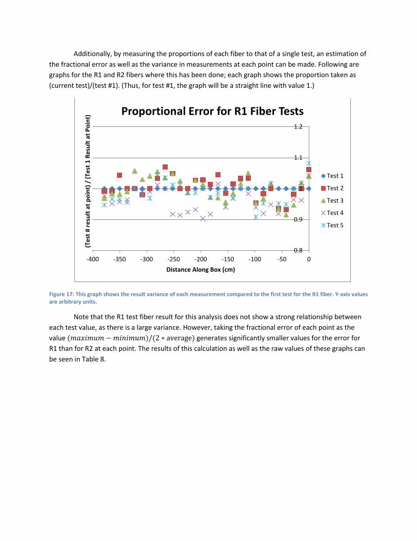
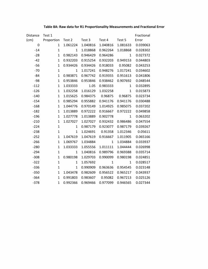
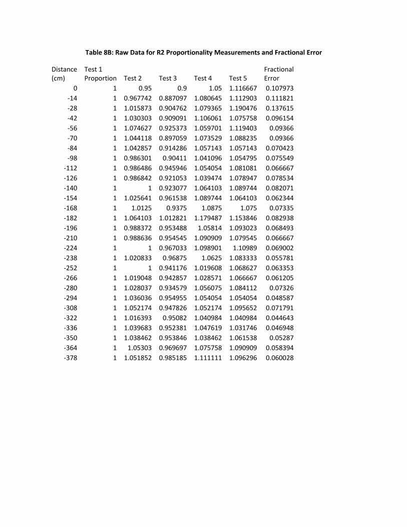
Additionally, by measuring the proportions of each fiber to that of a single test, an estimation of
the fractional error as well as the variance in measurements at each point can be made. Following are
graphs for the R1 and R2 fibers where this has been done; each graph shows the proportion taken as
(current test)/(test #1). (Thus, for test #1, the graph will be a straight line with value 1.)
Figure 17: This graph shows the result variance of each measurement compared to the first test for the R1 fiber. Y-axis values are arbitrary units.
Note that the R1 test fiber result for this analysis does not show a strong relationship between
each test value, as there is a large variance. However, taking the fractional error of each point as the
value generates significantly smaller values for the error for
R1 than for R2 at each point. The results of this calculation as well as the raw values of these graphs can
be seen in Table 8.
0.8
0.9
1
1.1
1.2
-400 -350 -300 -250 -200 -150 -100 -50 0
(Te
st #
re
sult
at
po
int)
/ (
Test
1 R
esu
lt a
t P
oin
t)
Distance Along Box (cm)
Proportional Error for R1 Fiber Tests
Test 1
Test 2
Test 3
Test 4
Test 5
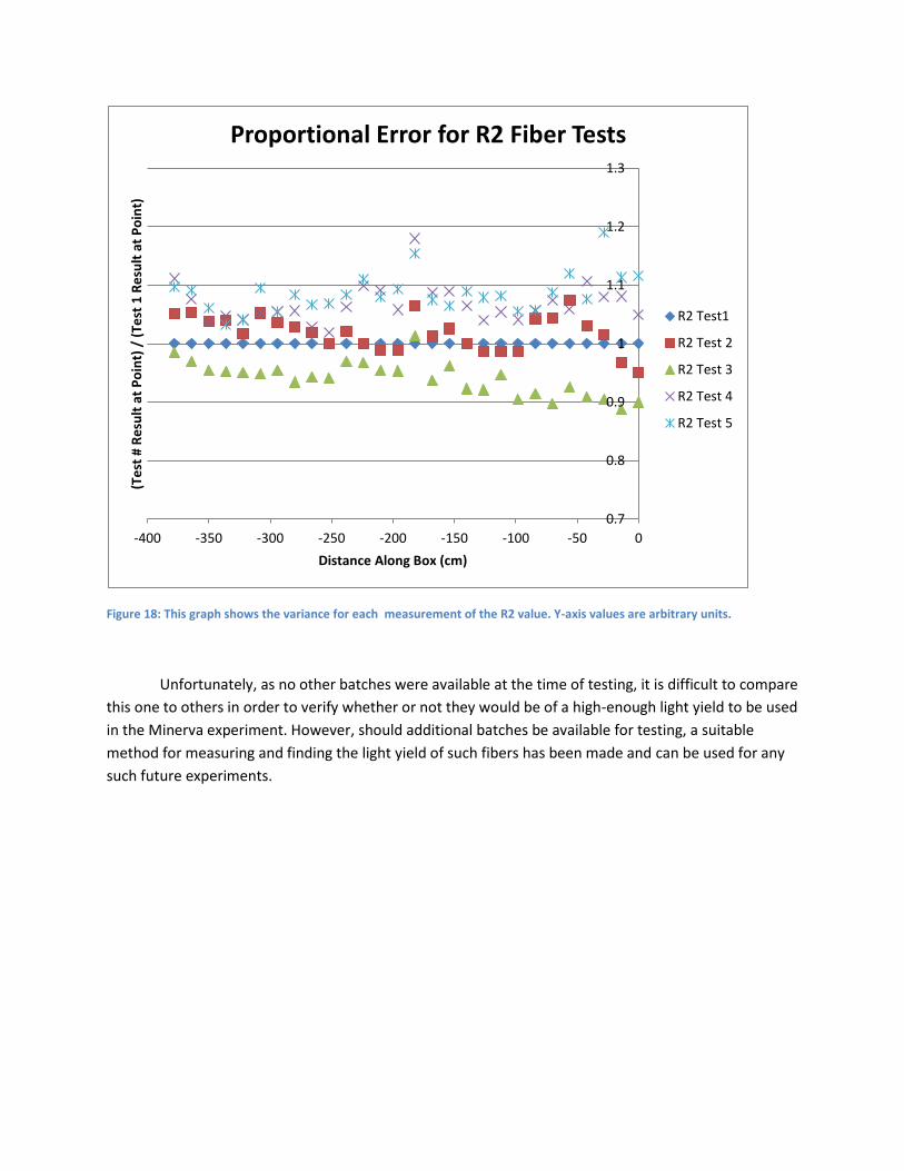
Figure 18: This graph shows the variance for each measurement of the R2 value. Y-axis values are arbitrary units.
Unfortunately, as no other batches were available at the time of testing, it is difficult to compare
this one to others in order to verify whether or not they would be of a high-enough light yield to be used
in the Minerva experiment. However, should additional batches be available for testing, a suitable
method for measuring and finding the light yield of such fibers has been made and can be used for any
such future experiments.
0.7
0.8
0.9
1
1.1
1.2
1.3
-400 -350 -300 -250 -200 -150 -100 -50 0
(Te
st #
Re
sult
at
Po
int)
/ (
Test
1 R
esu
lt a
t P
oin
t)
Distance Along Box (cm)
Proportional Error for R2 Fiber Tests
R2 Test1
R2 Test 2
R2 Test 3
R2 Test 4
R2 Test 5
Citations
Nelson, Jeffrey. The College of William and Mary. Personal Communication.
Appendix 1: C Source for Exponential Fit Data // global variables
TCanvas *canvas;
TGraph *graph;
TF1 *func;
void fit_expo(char *file, int color = kPink)
{
// open file
ifstream f(file);
if(f.fail())
{
cerr << "error: unable to open file \"" << file << "\"" << endl;
return;
}
// ignore first line
string s;
getline(f, s);
double dial, x, Iraw, I;
vector <double> xs;
vector <double> Is;
// read file
for(;;)
{
f >> dial >> x >> Iraw >> I;
if(f.eof() || f.fail()) break;
xs.push_back(-x);
Is.push_back(-I);
}
// close file
f.close();
// style
gROOT->SetStyle("Plain");
gStyle->SetPalette(1);
gStyle->SetMarkerStyle(kPlus);
gStyle->SetMarkerSize(1.5);
gROOT->ForceStyle();
// create canvas
bool canvas_exists = gROOT->FindObject("canvas");
if(!canvas_exists) canvas = new TCanvas("canvas", "canvas");
// create TGraph
double *xs_c = new double[xs.size()]; for(int i = 0; i < xs.size(); i++) xs_c[i] = xs[i];
double *Is_c = new double[Is.size()]; for(int i = 0; i < Is.size(); i++) Is_c[i] = Is[i];
graph = new TGraph(xs.size(), xs_c, Is_c);
graph->SetTitle(";x (cm);I (nA)");
graph->Draw((canvas_exists)? "P" : "AP");
delete[] xs_c;
delete[] Is_c;
// fit exponentials
func = new TF1("func", "[0]*(exp(-x/[2])+[1]*exp(-x/[3]))");
func->SetParNames("A", "B", "L1", "L2");
func->SetParameter(0, 2.0); // nA
func->SetParameter(1, 1.0); // nA
func->SetParameter(2, 50.0); // cm
func->SetParameter(3, 400.0); // cm
func->SetLineColor(color);
graph->Fit("func");
}
The previous is the source code used to create the exponential fits used in the graphs of the data for the R1, R2, and RG* fibers. It is designed to be used within ROOT. ROOT can be downloaded at http://root.cern.ch/drupal/content/downloading-root. Version 5.28/00 was used.
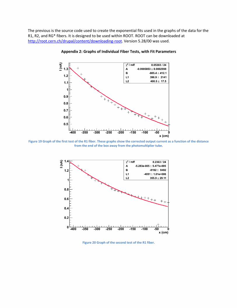
Appendix 2: Graphs of Individual Fiber Tests, with Fit Parameters
Figure 19 Graph of the first test of the R1 fiber. These graphs show the corrected output current as a function of the distance
from the end of the box away from the photomultiplier tube.
Figure 20 Graph of the second test of the R1 fiber.