Universite Joseph Fourier

Rapport de stage

Master 2 Recherche Mathematiques Appliquees

The adaptive fused lasso regressionand its application on microarrays

CGH data

Author :Mohamad Ghassany

Supervisor :Sophie Lambert-Lacroix

Grenoble

22 juin 2010

Acknowledgements

I would firstly like to thank Mme Sophie Lambert-Lacroix for her guidance, encou-ragement and good advice. This thesis is a much work better thanks to her supervision.

My thanks must also go to Mr. Eric Bonnetier, our responsible for master 2 researchfor his help and patience during this year.

I would also like to thank my family and friends for all their invaluable support.

1

Table des matieres

1 Introduction 3

2 The fused Lasso regression 5

2.1 Fused Lasso penalty . . . . . . . . . . . . . . . . . . . . . . . . . . . . . . 5

2.2 Adaptive fused Lasso penalty . . . . . . . . . . . . . . . . . . . . . . . . . 6

2.2.1 Adaptive Lasso and Oracle properties . . . . . . . . . . . . . . . . . 6

2.2.2 Adaptive fused Lasso . . . . . . . . . . . . . . . . . . . . . . . . . . 7

2.3 The FLSA and microarrays CGH . . . . . . . . . . . . . . . . . . . . . . . 8

2.4 The A-FLSA . . . . . . . . . . . . . . . . . . . . . . . . . . . . . . . . . . 9

2.4.1 The A-FLSA’s oracle properties . . . . . . . . . . . . . . . . . . . . 10

3 Path algorithm to solve the A-FLSA 12

3.1 Piecewise linear regularized solution path . . . . . . . . . . . . . . . . . . . 12

3.2 Path algorithm for the A-FLSA . . . . . . . . . . . . . . . . . . . . . . . . 14

4 Numerical Results 18

4.1 Simulations and noise . . . . . . . . . . . . . . . . . . . . . . . . . . . . . . 18

4.2 Cross Validation . . . . . . . . . . . . . . . . . . . . . . . . . . . . . . . . . 19

4.3 Comparing the performance of FLSA and A-FLSA . . . . . . . . . . . . . 20

4.3.1 False discovery rate . . . . . . . . . . . . . . . . . . . . . . . . . . . 20

4.3.2 Performance of FLSA and A-FLSA . . . . . . . . . . . . . . . . . . 23

4.3.3 Mean squared error . . . . . . . . . . . . . . . . . . . . . . . . . . . 23

4.4 Results . . . . . . . . . . . . . . . . . . . . . . . . . . . . . . . . . . . . . . 24

4.5 Comparison . . . . . . . . . . . . . . . . . . . . . . . . . . . . . . . . . . . 25

5 Conclusion and perspectives 27

A Appendix 28

2

1 Introduction

Statistics has been constantly challenged by issues raised in biological sciences. In

the early days many problems came from agricultural sciences and genetics, and the ex-

plosion of high-throughput technologies in “omics” molecular biology has extended the

scope of statistical needs in the last twenty years. A common characteristics of many

omics data is their large dimension compared to the relatively small number of samples

on which they are measured, leading to the famous “small n large p” problem. Conse-

quently statistical fields such as multiple testing, clustering, classification, regression, and

dimension reduction have been (re)investigated following questions raised by molecular

biologists (see for instance [7]). Sparse methods such as the Lasso for regression or the

Cox model ([10, 11, 2]), which estimate a function and select features at the same time,

have gained a lot of popularity in high-dimensional statistics in the last 10 years, although

their theoretical analysis is much more recent [14, 1]. Their wide diffusion has also been

supported by works on optimization. For instance the fused Lasso criterion leads to a

convex optimization problem which has been solved to provide a solution in much less

time that a standard convex optimizer [4]. Sparse methods have also been extended to

the analysis of piecewise-constant 1D profiles with the fused Lasso [12, 4], triggered by

applications in CGH profile analysis [13][8].

aCGH arrays have now become popular tools to identify DNA CNV along the ge-

nome. These profiles are used to identify genomic markers to improve cancer prognosis and

diagnosis. Like gene expression profiles, CNV profiles are characterized by a large number

of variables usually measured on a limited number of samples. In this part, we want to

develop methods for prognosis or diagnosis of patient outcome from CNV data. Due to

their spatial organization along the genome CNV profiles have a particular structure of

correlation between variables. This suggests that classical classification methods should

be adapted account for this spatial organization. To do so one can use penalties such as

the fused Lasso penalty. The Lasso penalty is a regularization technique for simultaneous

estimation and variable selection ([10]). It consists in the introduction of a l1-type penalty,

which enforces the shrinkage of coefficients. The fused Lasso was introduced by [12] ; it

3

combines a Lasso penalty over coefficients and a Lasso penalty over their difference, thus

enforcing similarity between successive features. One drawback of the Lasso penalty is

the fact that, since it uses the same tuning parameters for all regression coefficients, the

resulting estimators may suffer from an appreciable bias (see [3]). Moreover recent results

show that the underlying model must satisfy a nontrivial condition for the Lasso estima-

tor to be consistent (see [15]). Consequently in some cases the Lasso estimator can be

non-consistent. To fix this issue, a possibility is to introduce adaptive weights to penalize

different coefficients in the l1 penalty, as done in the adaptive Lasso which enjoys oracle

properties. Moreover, the adaptive Lasso can be solved by the same efficient algorithm

than the one used to solve the Lasso. Our claim is that the fused Lasso estimator will

suffer from the same defaults as the Lasso because it is based on the same l1 penalty,

suggesting that it may be interesting to adapt the adaptive approach of [15] to the fused

Lasso penalty. We will study the possibility to introduce adaptive weights in the fused

Lasso penalty, resulting in the adaptive fused Lasso penalty. In this report, we show in

details what the adaptive fused Lasso is, we give our attention to a special case of the

adaptive fused Lasso, the adaptive fused Lasso signal approximator (A-FLSA), we adapt

a path algorithm to solve the A-FLSA and we apply our algorithm on simulated data in

order to compare the fused Lasso and the adaptive fused Lasso.

4

2 The fused Lasso regression

2.1 Fused Lasso penalty

Consider the standard linear regression model

yi = α∗ + xTi β∗ + εi, i = 1, . . . , n. (2.1)

where xj = (x1j, . . . , xnj)T for j = 1, . . . , p are the regressors, α∗ is the constant para-

meter, β∗ = (β∗1 , . . . , β∗p)T are the associated regression coefficients and yi is the response

for the ith observation. Let X = [x1, . . . ,xp] be the predictor matrix, we also call it

design matrix, and let y = (y1, . . . , yn) the response vector. We suppose that the errors

εi are independent and identically-distributed (iid) Guassian random errors with mean 0

and constant variance σ2. We also assume that the predictors are standardized to have

mean zero and unit variance, and the outcome yi has mean zero. Hence we don’t need an

intercept α∗ in the model 2.1.

The unknown parameters in the model 2.1 are usually estimated by minimizing the Or-

dinary Least Squares (OLS) criterion, in which we seek to minimize the residual squared

error, but there are two reasons why the data analyst is often not satisfied with the OLS

estimates.

1. prediction accuracy the OLS estimates often have low bias but large variance.

2. interpretation with a large number of predictors, we often would like to determine a

smaller subset that exhibits the strongest effects, but it is computationally infeasible

to do subset selection in this case.

Prediction accuracy can sometimes be improved by shrinking or setting to 0 some coeffi-

cients. By doing so we sacrifice a little bias to reduce the variance of the predicted values

and hence may improve the overall prediction accuracy. For this, Tibshirani [10] proposed

a new technique, called the Lasso, for “least absolute shrinkage and selection operator”.

It shrinks some coefficients and sets others to 0.

Letting β = (β1, . . . , βp)T the estimated vector of β, the Lasso estimate β minimizes

5

the following problem in the “Lagrange” form

f(β) =1

2

n∑i=1

(yi −

p∑j=1

xijβj

)2

+ λ1

p∑j=1

|βj|, (2.2)

where λ1 is a nonnegative regularization parameter. The second term in 2.2 is the so-called

“l1 penaly”. The Lasso continuously shrinks the coefficients toward 0 as λ1 increases, and

some coefficients are shrunk to exact 0 if λ1 is sufficiently large. The Lasso has a unique

solution assuming no two predictors are perfectly collinear. One drawback of the Lasso is

the fact that it ignores ordering of the features, of the type of data we are working on in

this report, the microarrays comparative genomic hybridization (microarrays CGH). For

this purpose, Tibshirani [12] proposed the fused Lasso, which combines a Lasso penalty

over coefficients and a Lasso penalty of their difference. The fused Lasso criterion is defined

by

f(β) =1

2

n∑i=1

(yi −

p∑j=1

xijβj

)2

+ λ1

p∑j=1

|βj|+ λ2

p−1∑j=1

|βj − βj+1|. (2.3)

The first penalty encourages sparsity in the coefficients, the second penalty encourages

sparsity in their differences, therefore as λ1 and λ2 increase, some coefficients are shrunk

to 0 and some consecutive coefficients are shrunk to be equal to each other, thus enforcing

similarity between successive features.

2.2 Adaptive fused Lasso penalty

Recent studies showed that the resulting estimators of the Lasso may suffer from

an appreciable bias. Moreover, they showed that the underlying model must satistfy a

nontrivial condition for the Lasso estimator to be consistent (Zou [15]). In his paper

[15], Zou proposed a new version of the Lasso, called the adaptive Lasso, where adaptive

weights are used for penalizing different coefficients in the l1 penalty. He showed that the

adaptive Lasso enjoys the oracle properties.

2.2.1 Adaptive Lasso and Oracle properties

Consider the standard linear regression model 2.1. We assume that the data are

centered, so the intercept α∗ is not included in the regression function. Let A = {1 ≤j ≤ p, β∗j 6= 0} and p0 = |A| the cardinal of A. We assume that p0 < p. Thus the true

model depends only on a subset of the predictors. Denote by β(δ) the coefficient estimator

produced by a fitting procedure δ. Using the language of Fan and Li [3], we call δ an oracle

6

procedure if β(δ) (asymptotically) satisfies the following oracle property :

– Consistency in variable selection : limn P(A∗ = A) = 1,

where A∗ = {j : βj(δ) 6= 0}.It has been argued (Fan and Li [3]) that a good procedure should have these oracle

properties. Fan and Li [3] studied a class of penalization methods including the Lasso.

They showed that the Lasso shrinkage produces biased estimates for the large coefficients,

and thus it could be suboptimal in terms of estimation risk. Fan and li [3] conjectured

that the oracle propeties do not hold for the Lasso. Then Zou [15] showed that the Lasso

variable selection can be inconsistent in some scenarios.

Basing on the aboved, Zou [15] derived a necessary condition for the Lasso variable

selection to be consistent. He proposed a new version of the Lasso, called the adaptive

Lasso where adaptive weights are used for penalizing different coefficients in the l1 penalty.

He also showed that the adaptive Lasso enjoys the oracle properties. Let us consider the

weighted Lasso, by adding those weights the equation 2.2 that we seek to minimize in the

Lasso problem become

f(β) =1

2

n∑i=1

(yi −

p∑j=1

xijβj

)2

+ λ1

p∑j=1

wj|βj|, (2.4)

where w = (w1, . . . , wp) is a known weights vector. Zou [15] showed that if the weights are

data-dependent and cleverly chosen, the weighted Lasso can have the oracle properties.

He called this methodology the adaptive Lasso.

So, in order to choose the appropriate weights, consider βols the ordinary least squares

estimator of β∗, which is a root-n-consistent estimator to β∗. Pick a γ > 0, therefore we

define the weight vector as w = |βols|−γ, which is well data-dependent.

2.2.2 Adaptive fused Lasso

Now back to the fused Lasso 2.3 proposed by Tibshirani [12], the fused Lasso will

suffer from the same defaults as the Lasso since it is based on the same l1 penalty. The-

refore, we will introduce some weights in the fused Lasso model, as same as Zou [15] did

with the Lasso problem. Precisely we propose the following criterion

f(β) =1

2

n∑i=1

(yi −

p∑j=1

xijβj

)2

+ λ1

p∑j=1

w(1)j |βj|+ λ2

p−1∑j=1

w(2)j |βj − βj+1|, (2.5)

where w(1) = |βj|−γ, j = 1, . . . , p and w(2) = |βj − βj+1|−γ, j = 1, . . . , p− 1 are the

7

weights vectors. Note that β here is always the estimate of β∗ obtained by OLS, β = βols.

In this report we will pick γ = 1.

2.3 The FLSA and microarrays CGH

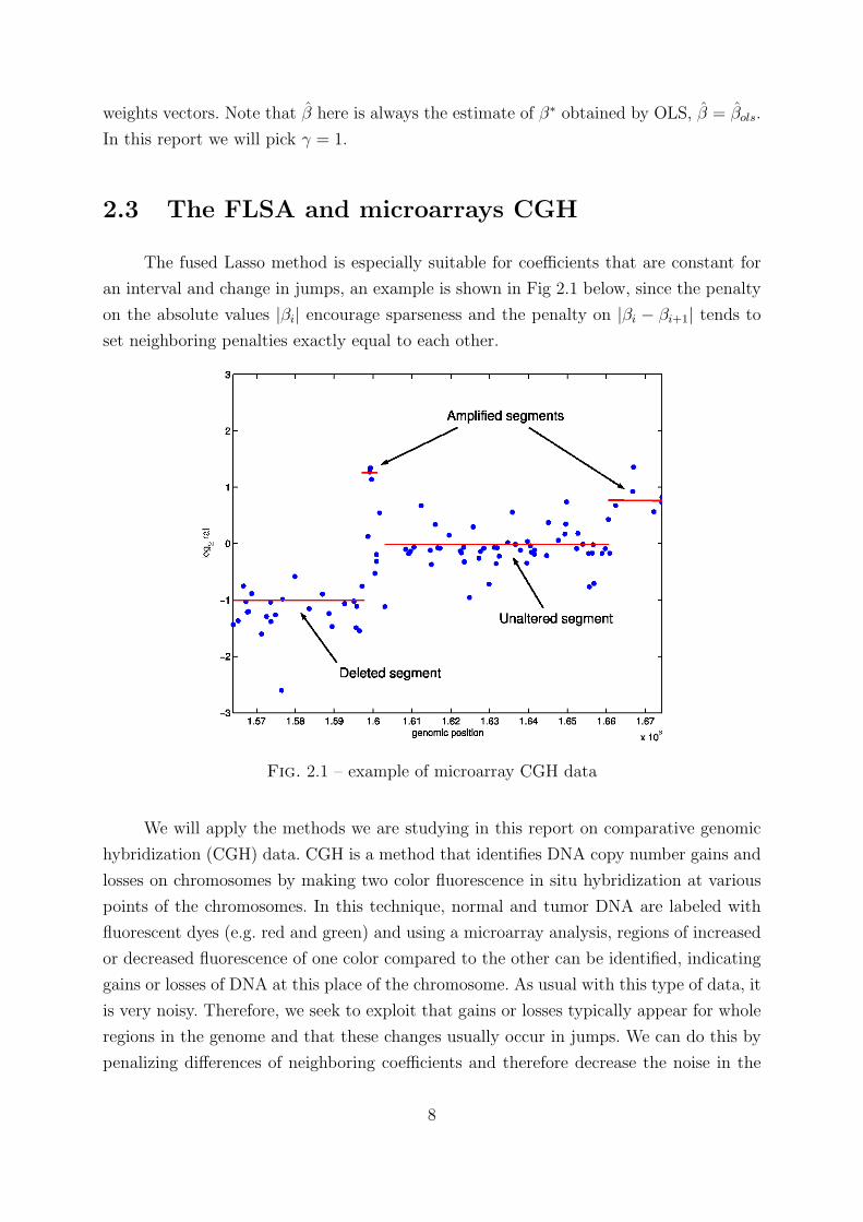
The fused Lasso method is especially suitable for coefficients that are constant for

an interval and change in jumps, an example is shown in Fig 2.1 below, since the penalty

on the absolute values |βi| encourage sparseness and the penalty on |βi − βi+1| tends to

set neighboring penalties exactly equal to each other.

Fig. 2.1 – example of microarray CGH data

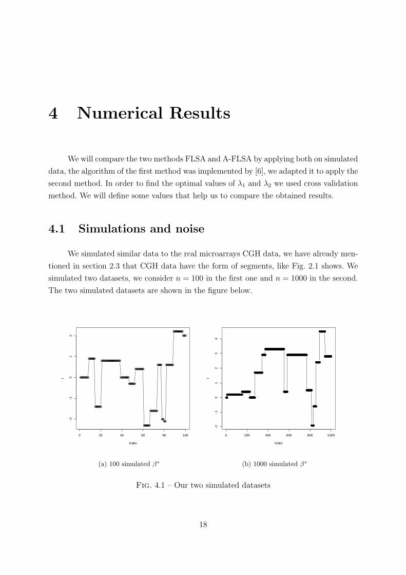
We will apply the methods we are studying in this report on comparative genomic

hybridization (CGH) data. CGH is a method that identifies DNA copy number gains and

losses on chromosomes by making two color fluorescence in situ hybridization at various

points of the chromosomes. In this technique, normal and tumor DNA are labeled with

fluorescent dyes (e.g. red and green) and using a microarray analysis, regions of increased

or decreased fluorescence of one color compared to the other can be identified, indicating

gains or losses of DNA at this place of the chromosome. As usual with this type of data, it

is very noisy. Therefore, we seek to exploit that gains or losses typically appear for whole

regions in the genome and that these changes usually occur in jumps. We can do this by

penalizing differences of neighboring coefficients and therefore decrease the noise in the

8

data and improve estimation. We concentrate on the most widely used case for the fused

Lasso method, the Fused Lasso Signal Approximator (FLSA). In the FLSA, we assume

that we have X = I as the predictor matrix and that we have n = p. Therefore the loss

function 2.3 becomes

f(β) =1

2

n∑i=1

(yi − βi)2 + λ1

n∑i=1

|βi|+ λ2

n−1∑i=1

|βi − βi+1|. (2.6)

Every coefficient βi is an estimate of the measurement yi taken at position i (which we

assume to be ordered along the chromosome). Apart from the Lasso penalty λ1

∑ni=1 |βi|,

the additional penalty placed on the difference between neighboring coefficients is

λ2

∑n−1i=1 |βi − βi+1|. An example of CGH measurements in lung cancer can be seen in

Fig 2.2. The red line are the estimates for penalty parameters λ1 = 0 and λ2 = 2. We

can see that starting around measurement 150, the CGH results are on average below 0,

indicating a loss of DNA in this region.

Fig. 2.2 – Example using the one-dimensional Fused Lasso Signal Approximator on lungcancer CGH data.

2.4 The A-FLSA

As we already mentioned in section 2.2.3 about the fused Lasso model, it will suffer

from some defaults, we proposed to add weights in the criterion in order to avoid these

9

defaults, so we will do the same for the FLSA, we will add those weights in the equation

2.6. We will call it the “Adaptive Fused Lasso Signal Approximator” (A-FLSA). The loss

function 2.6 we seek to minimize becomes

f(β) =1

2

n∑i=1

(yi − βi)2 + λ1

n∑i=1

w(1)i |βi|+ λ2

n−1∑i=1

w(2)i |βi − βi+1|, (2.7)

where the weights are the same defined above.

In the next chapter, we will explore a path algorithm to solve the A-FLSA, then we will

use cross-validation to find the optimal values of λ1 and λ2.

2.4.1 The A-FLSA’s oracle properties

To verify that we can use the A-FLSA, we must be sure that it enjoys the oracle

properties (see section 2.2.1). Zou [15] gave a necessary condition to the consistency of

the Lasso selection, it also can be a necessary condition of the A-FLSA since it is based

on the same penalty. We assume that we have the model presented in 2.1 without the

intercept, and that 1nXTX→ C where C is a positive definite matrix.

Without loss of generality, assume that A = {1, 2, . . . , p0}. Recall that A = {j : β∗j 6= 0}.Let

C =

[C11 C12

C21 C22

]

where C11 is a p0 × p0 matrix. Let β the A-FLSA estimates, obtained by minimizing

equation 2.7. Recall that A∗ = {j : βj 6= 0}. The necessary condition presented in [15] is

the following

– Suppose that limn P(A∗ = A) = 1. Then there exists some sign vector s =

(s1, . . . , sp0)T , sj = 1 or −1, such that

|C21C−111 s| ≤ 1 (2.8)

Zou [15] showed that if condition 2.8 fails, then the Lasso variable selection is inconsistent.

He found an example where condition 2.8 cannot be satistied.

As for the A-FLSA, we have always X = I the design matrix. In this case, the

condition 2.8 is satisfied since |C21C−111 s| in this case is always 0, thus it is ≤ 1. Therefore,

we satisfy the necessary condition but we can say nothing more about the consistency of

the A-FLSA, so we are not quite sure that the A-FLSA enjoys the oracle properties.

In perspective, it will be interesting to find a necessary condition for the consistency of

the adaptive fused Lasso variable selection in the case of random X as a design matrix,

10

especially trying to find what kind of hypotheses we need to propose, since we penalize

an additional term in the fused Lasso, the absolute value of difference of coefficients.

11

3 Path algorithm to solve the

A-FLSA

We consider the generic regularized optimization problem β(λ1) =

argminβL(y,Xβ) + λ1J(β) that is the case of the Lasso problem. Efron et al.[2] have

shown that for the Lasso, that is if L is squared error loss and J(β) = ‖β‖1 =∑p

i=1 |βi|is the l1 norm of β if its length is p, the optimal coefficient path is piecwise linear, i.e.,

∂β(λ1)/∂λ1 is piecewise constant. Rosset and Zhu [9] derived a general characterization

of the properties of (loss L, penalty J) pairs which give piecewise linear coefficient paths.

Such pairs allow for efficient generation of the full regularized coefficient paths.

3.1 Piecewise linear regularized solution path

Regularization is an essential component in modern data analysis, in particular

when the number of predictors is large, possibly larger than the number of observations,

and non-regularized fitting is likely to give badly over-fitted and useless models. We will

concentrate on a special case of the generic regularized optimization problems which is

the Lasso, and later on its generalizations, the fused Lasso and the adaptive fused Lasso.

The inputs we have in the Lasso are :

– A data sample X and the response vector y as described in chapter 2.

– A convex non-negative loss functional L : Rn × Rn → R.

– A convex non-negative penalty functional J : Rp → R, with J(0) = 0.

We want to find :

β(λ1) = argminβ∈RpL(y,Xβ) + λ1J(β), (3.1)

where λ1 ≥ 0 is the regularization parameter, λ1 = 0 corresponds to no regularization,

while limλ1→∞ β(λ1) = 0.

The Lasso uses squared error loss as L and the l1 norm as the penalty J , therefore we

12

write 3.1 as,

β(λ1) = minβ

n∑i=1

(yi − xTi β)2 + λ1

p∑i=1

|βi|. (3.2)

Many “modern” methods for machine learning, signal processing and statistical modeling

can also be cast in the framework of regularized optimization. For example, the regularized

support vector machine, the ridge regression and the penalized logistic regression.

For the coefficient paths to be piecewise linear, we require that ∂β(λ1)∂λ1

/‖∂β(λ1)∂λ1‖ is

a piecewise constant vector as a function of λ1. [9] showed two sufficient conditions for

piecewise linearity :

– L is piecewise quadratic as a funtion of β along the optimal path β(λ1), when

X, y are assumed constant at their sample valures.

– J is piecewise linear as a function of β along this path.

We concentrate our attention on (loss L, penalty J) pairings where the optimal

path β(λ1) is piecewise linear as a funtion of λ1, i.e., ∃λ(0)1 = 0 < λ

(1)1 < . . . < λ

(m)1 = ∞

and γ0, γ1, . . . , γm−1 ∈ Rp such that β(λ1) = β(λ(k)1 ) + (λ1−λ(k)

1 )γk for λ(k)1 ≤ λ1 ≤ λ

(k+1)1 .

Such models are attractive because they allow us to generate the whole regularized path

β(λ1), for 0 ≤ λ1 ≤ ∞, simply by sequentially calculation the “step sizes” between each

two consecutive λ1 values and the “directions” γ1, . . . , γm−1. A canonical example is the

Lasso 3.2. In 2004, [2] have shown that the piecewise linear coefficient paths property

holds for the Lasso.

As for the fused Lasso, it is obvious that the piecewise linear coefficient paths pro-

perty holds. The difference we have is that β depends on two values λ1 and λ2 instead of

just λ1, with adding a second term on the regularized optimization problem, which is the

penalty on the differences of consecutive values of β. Let us call J1(β) =∑p

i=1 |βi| and

J2(β) =∑p−1

i=1 |βi − βi+1|, in the fused Lasso we want to find

β(λ1, λ2) = argminβ∈RpL(y,Xβ) + λ1J1(β) + λ2J2(β). (3.3)

As for the adaptive fused Lasso, nothing will be changed since the weights we consi-

der are constant and do not affect on the piecewise linearity of J1(β) and J2(β). Therefore,

we will use a path algorithm to solve the A-FLSA.

13

3.2 Path algorithm for the A-FLSA

In his paper, Hoefling [6] described a path algorithm that solves the FLSA. We

adapted this algorithm in order to solve the A-FLSA. We will desribe the algorithm in

this section. An important clue of this algorithm is that due to the simple structure of the

loss function 2.7, it is possible in this case to obtain the solution for any value of (λ1,λ2)

by simple soft-thresholding of the solution obtained for (0, λ2). To be more precise, the

following theorem holds :

Theorem 1. Assume we have X = I and that the solution for λ1 = 0 and λ2 > 0 is

known and denote it by β(0, λ2). Then the solution for λ1 > 0 is

βi(λ1, λ2) = S(βi(0, λ2), w(i)1 λ1)

= sign(βi(0, λ2)) (|βi(0, λ2)| − w(i)1 λ1)

+ for i = 1, · · · , p

where y+ = max(0, y).

The proof of this theorem is presented in the appendix. For the rest of this section,

we assume that λ1 = 0. The algorithm presented is a path algorithm that finds the solution

for all possible values of λ2. Any solution for a λ1 6= 0 can then be obtained by simply

soft-thresholding as shown above. Therefore the criterion we want to minimize becomes

L(y, β) =1

2

n∑i=1

(yi − βi)2 + λ2

n−1∑i=1

w(2)i |βi − βi+1|, (3.4)

where w(2)i = |βi − βi+1|−1.

The path algorithm will start by setting λ2 = 0 and then increase it until all coefficients

βi have the same value. For increasing λ2 neighboring coefficients are forced to be equal to

each other. Once this happens, these coefficients are being fused and subsequently treated

as a single variable for increasing λ2. In order to be able to do this, a special result holds

for the FLSA, that makes the algorithm especially simple and also has been presented

and proved in [4]. It states that if coefficients are fused at λ02 , then these coefficients will

also be fused for any λ2 > λ02. To be more precise

Theorem 2. Let βk(0, λ2) be the optimal solution to the A-FLSA problem for coefficient k

and penalty parameter λ2. Then if for some k and λ02 it holds that βk(0, λ

02) = βk+1(0, λ

02),

then for any λ2 > λ02 it holds that βk(0, λ2) = βk+1(0, λ2).

14

The algorithm

In order to develop the algorithm, we first have to define what exactly the sets of

fused coefficients are.

Definition 1. ([6]) Let Fi i = 1, · · · , nF (λ2) be the set of coefficients at λ2 that are

considered to be fused, where nF (λ2) is the number of such sets. In order for these sets to

be valid, we will write every set Fi in the form of Fi = {k|li ≤ k ≤ ui} and the following

statements have to hold :

– ∪nF (λ2)i=1 Fi = 1, · · · , n.

– Fi ∩ Fj = ∅, i 6= j.

– Assuming the Fi are ordered, for every k, l ∈ Fi we have βk(λ2) = βl(λ2) and for

k ∈ Fi, l ∈ Fi+1 it holds that βk(λ2) 6= βl(λ2).

For notational convenience, we will write βFi(λ2) for any βk(λ2) with k ∈ Fi and

also suppress the dependency of Fi onto λ2. Using this definition of fused sets, let us now

turn to the algorithm.

The algorithm is too simple due to Theorem 1 and Theorem 2. First, we need a starting

point for the path algorithm and as the optimal solution is known for λ2 = 0, which is

just βk(0) = yk for all k, we use it to begin the path. Then the algorithm calculates step

by step when two neighboring sets have equal coefficients and merges them.

Now let us introduce the loss function that incorporates the fused sets Fi, we will

call it LF,λ2 . This is done by taking the loss function L in equation 3.4 and replacing βk

by βFi for k ∈ Fi. This constrained loss function is then

LF,λ2(y, β) =1

2

nF (λ2)∑i=1

(∑j∈Fi

(yj − βFi)2

)+ λ2

nF (λ2)−1∑i=1

|βFi − βFi+1|

|βmaxFi − βminFi+1|. (3.5)

Note that Fi contains the indices of the coefficients βk that are fused at the corresponding

value λ2, thus the term |βmaxFi−βminFi+1|−1 is the appropriate weight to adapt |βFi−βFi+1

|,so βmaxFi is the OLS estimate of β∗maxFi .

This constrained loss function 3.5 is always differentiable with respect to βFi due

to the assumptions on the sets F. To get an optimal solution of βFi , we will calculate

the derivative of LF,λ2 with respect to βFi and find its root. The derivative of LF,λ2 for

i = 1, . . . , nF (λ2) is

∂LF,λ2

∂βFi= (#Fi)βFi −

∑j∈Fi

yj + λ2

sign(βFi − βFi−1)

|βmaxFi−1− βminFi |

+ λ2

sign(βFi − βFi+1)

|βmaxFi − βminFi+1|, (3.6)

15

where #Fi is the cardinal of Fi. We set sign(βF1 − βF0) = 0 and sign(βFnF (λ2)−

βFnF (λ2)+1) = 0 since βF0 and βFnF (λ2)+1

do not exist.

Then by putting ∂LF,λ2/∂βFi = 0 the optimal value of βFi for i = 1, . . . , nF (λ2) is

βFi(λ2) =1

#Fi

[∑j∈Fi

yj − λ2(sign(βFi − βFi−1

)

|βmaxFi−1− βminFi |

+sign(βFi − βFi+1

)

|βmaxFi − βminFi+1|)

]. (3.7)

We will calculate the derivative of βk(λ2) with respect to λ2 and we will see that these

are actually constant, so that the resulting solution path is a piecewise linear function [9]

where the breakpoints occur when two sets of coefficients are being fused. The derivative

of βk(λ2) for i = 1, . . . , nF (λ2) is

∂βFi∂λ2

= − 1

#Fi

(sign(βFi − βFi−1

)

|βmaxFi−1− βminFi |

+sign(βFi − βFi+1

)

|βmaxFi − βminFi+1|

). (3.8)

These derivatives are constant as long as the sets of fused coefficients do not change.

By Theorem 2, we know that only way to change the sets of fused coefficients is to merge

two sets as they can never split for increasing λ2. Therefore, the solution path is piecewise

linear and for increasing λ2 the breakpoint occurs when two groups fuse. Thus, it is

easy to calculate the next breakpoint, which occurs when neighboring sets have the same

coefficients. In order to do this, define

hi,i+1(λ2) =βFi(λ2)− βFi+1

(λ2)∂βFi+1

∂λ2− ∂βFi

∂λ2

+ λ2 for i = 1, . . . , nF (λ2)− 1.

which is the value for λ2 at which the coefficients of the sets Fi and Fi+1 have the same

value and can be fused, assuming that no other coefficients become fused before that. If

hi,i+1(λ2) < λ2, these values are being ignored as the two groups Fi and Fi+1 are actually

moving apart for increasing λ2. The next value at which coefficients are fused is therefore

the hitting time

h(λ2) = minhi,i+1(λ2)>λ2

hi,i+1(λ2).

As we taking the minimum, it is only defined if there is at least one hi,i+1(λ2) > λ2. From

equation (2.2) with λ1 = 0 we can easily see that for λ2 →∞ the solution is βk = 1n

n∑l=1

yl

for all k, thus only one group exists for large λ2. Therefore, if nF (λ2) ≥ 2, then there

exists hi,i+1(λ2) > λ2 and therefore h(λ2) is defined. Based on this results, we write the

details of the algorithm that provides the entire solution path and the can be found in

Algorithm 1.

16

Algorithm 1: One-dimensional FLSA path algorithm

beginλ2 = 0 ;

βk = yk for k = 1, · · · , n ;

Fi = {i} for i = 1, · · · , n ;

nF = n ;

end

while nF > 1 doCalculate next hitting time h(λ2) ;

Let (i0(λ2), i0(λ2) + 1) = argmin hi,i+1>λ2hi,i+1(λ2) be the indices of the sets to

be fuse next ;

Fuse the two sets Fi0(λ2) and Fi0(λ2)+1 ;

Set : λ2 = h(λ2) ;

Update the values for βk(λ2),∂βk(λ2)∂λ2

and set nF = nF − 1 ;

end

17

4 Numerical Results

We will compare the two methods FLSA and A-FLSA by applying both on simulated

data, the algorithm of the first method was implemented by [6], we adapted it to apply the

second method. In order to find the optimal values of λ1 and λ2 we used cross validation

method. We will define some values that help us to compare the obtained results.

4.1 Simulations and noise

We simulated similar data to the real microarrays CGH data, we have already men-

tioned in section 2.3 that CGH data have the form of segments, like Fig. 2.1 shows. We

simulated two datasets, we consider n = 100 in the first one and n = 1000 in the second.

The two simulated datasets are shown in the figure below.

●●●●●●●●

●●●●●●

●●●●●●

●●●●●●●●●●●●●●●●●●

●●●●●●●●

●●●●●●

●●●●●●●●

●●●●●●

●●●●●●●

●●●●

●●●●

●●●●●●●

●●●●●●●●●

●●●

0 20 40 60 80 100

−2

−1

01

2

Index

f

(a) 100 simulated β∗

●●●●●●●●●

●●●●●●●●●●●●●●●●●●●●●●●●●●●●●●●●●●●●●●●●●●●●●●●●●●●●●●●●●●●●●●●●●●●●●●●●●●●●●●●●●●●●●●●●●●●●●●●●●●●●●●●●●●●●●●●●●●●●●●●●●●●●●●●●●●●●●●●●●●●●●●

●●●●●●●●●●●●●●●●●●●●●●●●●●●●●●●●●●●●●●●●●●●●●●●●●●●●●●●●●●●●●●●●●●●●●●●●●●

●●●●●●●●●●●●●●●●●●●●●●●●●●●●●●●●●●●●●●●●●●●●●●●●

●●●●●●●●●●●●●●●●●●●●●●●●●●●●●●●●●●●●●●●●●●●●●●●●●●●●●●●●●●●●●●●●●●●●●●●

●●●●●●●●●●●●●●●●●●●●●●●●●●●●●

●●●●●●●●●●●●●●●●●●●●●●●●●●●●●●●●●●●●●●●●●●●●●●●●●●●●●●●●●●●●●●●●●●●●●●●●●●●●●●●●●●●●●●●●●●●●●●●●●●●●●●●●●●●●●●●●●●●●●●●●●●●●●●●●●●●●●●●●●●●●●●●●●●●●●●●●●●●●●●●●●●●●●●●●●●●●●●●●●●

●●●●●●●●●●●●●●●●●●●●●●●●●●●●●●●

●●●●●●●●●●●●●●●●●●●●●●●●●●●●●●●●●●●●●●●●●●●●●●●●●●●●●●●●●●●●●●●●●●●●●●●●●●●●●●●●●●●●●●●●●●●●●●●●●●●●●●●●●●●●●●●●●●●●●●●●●●●●●●●●●●●●●●●●●●●●●●●●●●●●●●●●●●●●●●●●●●●●●●●●●●●●●●●●●●●●●●●●●

●●●●●●●●●●●●●●●●●●●●●●●●●●●●●●●●●●●●●●●●●●●●●●●

●●●●●●●●●●●●●●●●●●●

●●●●●●●●●●●●●●●●●●●●●●●●

●●●●●●●●●●●●●●●●●●●●●●●●●●●●●●●●●●

●●●●●●●●●●●●●●●●●●●●●●●●●●●●●●●●●●●●●●●●●●●●●●●●●●

●●●●●●●●●●●●●●●●●●●●●●●●●●●●●●●●●●●●●●●●●●●●●●●●●●●●●●●●●●●

0 200 400 600 800 1000

−2

−1

01

23

4

Index

f

(b) 1000 simulated β∗

Fig. 4.1 – Our two simulated datasets

18

Back to the initial model (2.1), we supposed that X = I as the design matrix and

that p = n, therefore we write the model as

yi = β∗i + εi i = 1, . . . , n.

We also supposed that the errors εi are iid with mean 0 and constant variance σ2. So

we must add some noise on the simulated datasets. To do so, we choose several level of

noise, we calculate three different values of σ, corresponding to three values of Signal-to-

Noise Ratio (SNR) given respectively 3, 5 and 7. The relation between σ and SNR is the

following

σ2 =1

n

‖β∗‖22SNR2

.

where ‖β∗‖22 =∑n

i=1(β∗i )

2. Therefore, if SNR=3, σ is high and the model is very noisy. If

SNR=7, the model is less noisy. For each simulated dataset, we repeated the adding noise

process 500 times, for three different levels of noise.

4.2 Cross Validation

Now in order to find the optimal values of λ1 and λ2 in both of FLSA and A-FLSA,

we tried two methods, the Bayesian Information Criterion (BIC) and cross validation.

After some tries on many randomly choosed simulations, we found that BIC does not give

us the optimal values, so we used cross validation.

Cross validation is a technique for assessing how the results of a statistical analysis

will generalize to an independent data set. It is mainly used in settings where the goal

is prediction, and one wants to estimate how accurately a predictive model will perform

in practice. Cross validation involves partitioning a sample of data into complementary

subsets, performing the analysis on one subset (called the training set), and validating

the analysis on the other subset (called the validation set or testing set).

Let yi one of the 500 simulations and we want to find the optimal values of λ1 and λ2 for

whose we have the best estimated β using either FLSA or A-FLSA. For instance, suppose

that we are in the case of n = 100, so we divide yi into two subsets. The first subset is

the testing set, we will call it y(T ), and it is in the form

y(T ) = {yi, i = 2k, k = 1, . . . , 50}.

The second subset is the training set, we will call it y(L), it contains the other elements

of yi, therefore

y(L) = {yi, i = 2k + 1, k = 0, . . . , 49}.

19

We will apply the regression FLSA and A-FLSA on the training set on a grill of values of

λ1 and λ2. For each pair (λ1,λ2) we find the estimated parameters, let βLλ1,λ2the vector of

these estimates. Then we calculate the Mean Squared Error (MSE) which is in this case

MSE(λ1,λ2) =50∑i=1

(y(T )i − β

(L)iλ1,λ2

)2 for every pair (λ1, λ2).

Therefore, the optimal values of λ1 and λ2 correspond to the minimal value of MSE.

(λ1, λ2) = argmin(λ1,λ2)MSE.

4.3 Comparing the performance of FLSA and A-

FLSA

Our objective is to compare the performance of the two methods FLSA and A-FLSA,

i.e., it is about multiple tests comparison. Statisticians were always interested by finding

an error rate to compare multiple tests, one of the most important rates discovered is the

false discovery rate (FDR). We will use this rate and another one, the false negative rate

(FNR) to compare the performance of FLSA and A-FLSA on simulated data. We will

also compare the important mean squared error (MSE) in both of FLSA and A-FLSA.

4.3.1 False discovery rate

In many multiplicity problems the number of erroneous rejections should be taken

into account and not only the question whether any error was made. Yet, at the same

time, the seriouness of the loss incurred by erroneous rejections is inversely related to the

number of hypotheses rejected. From this point of view, a desirable error rate to control

may be the expected proportion of errors among the rejected hypotheses, which is the

false discovery rate (FDR).

To be more specific, consider the problem of testing simultaneously m (null) hypotheses,

of which m0 are true, R is the number of hupotheses rejected. Table 4.1 summarizes the

situation in a traditional form.

20

Tab. 4.1 – Number of errors committed when testing m null hypotheses

Declared non-significant Declared significant TotalTrue null hypotheses U V m0

Non-true null hupotheses T S m−m0

m - R R m

The specific m hypotheses are assumed to be known in advance. R is an observable

random variable ; U, V, S and T are unobservable random variables. The proportion of

errors committed by falsely rejecting null hypotheses can be viewed through the random

variable Q = V/(V + S), the proportion of the rejected null hypotheses which are erro-

neously rejected. Q is an unobserved (unknown) random variable. FDR is defined to be

the expectation of Q,

FDR = E(Q) = E[V

V + S] = E(

V

R).

Classically, in segmentation we compute some metrics and we calculate FDR using

these metrics. To be more clear, we will explain how to evaluate the performance of a

classifier, note that we are not in a classification problem, segmentation is what does

interest us, but this explanation will helps us to understand where do these metrics come

from.

Classifier performance

A classification model (classifier or diagnosis) is a mapping of instances into a

certain class. Let us consider a two-class prediction problem (binary classification), in

which the outcomes are labeled either as positive (p) or negative (n) class. There are four

possible outcomes from a binary classifier. If the outcome from a prediction is p and the

actual value is also p, then it is called a true positive (TP) ; however if the actual value

is n then it is said to be a false positive (FP). Conversely, a true negative has occurred

when both the prediction outcome and the actual value are n, and false negative is when

the prediction outcome is n while the actual value is p. To get an appropriate example in

a real-world problem, consider a diagnostic test that seeks to determine whether a person

has a certain disease. A false positive in this case occurs when the person tests positive,

but actually does not have the disease. A false negative, on the other hand, occurs when

the person tests negative, suggesting they are healthy, when they actually do have the

disease.

Given a classifier and a set of instances (the test set), a two-by-two confusion matrix

21

(also called contingency table) can be constructed representing the dispositions of the set

of instances. This matrix forms the basis for many common metrics.

Fig. 4.2 – Confusion matrix

Looking at Table 4.1 and Figure 4.2, we can declare that,

– m0 is the number of true null hypotheses.

– m−m0 is the number of false null hypotheses.

– U is the number of true negatives.

– V is the number of false positives.

– T is the number of false negatives.

– S is the number of true positives.

Now we can define what exactly FDR is in our situation,

FDR =FP

FP + TP

Another error rate is defined and can be used, but staticians do not give it such big

importance, is the false negative rate (FNR), which is

FNR =FN

FN + TN

22

4.3.2 Performance of FLSA and A-FLSA

Now back to FLSA and A-FLSA, we have two-class prediction problem, but since

we putted two penalties, the first one on the absolute values of coefficients, the second

one on their difference, therefore for every metric of the described above, we will calculate

two values, one due the first penalty and one due the second penalty. Recall that we have

the model 2.1, so β∗ is the actual value and β is the outcome, therefore

False positives

FP1 = #{j : β∗j = 0 & βj 6= 0} (The cardinal of this set)

FP2 = #{j : β∗j = β∗j+1 & βj 6= βj+1}

False negatives

FN1 = #{j : β∗j 6= 0 & βj = 0}

FN2 = #{j : β∗j 6= β∗j+1 & βj = βj+1}

True positives

TP1 = #{j : β∗j 6= 0 & βj 6= 0}

TP2 = #{j : β∗j 6= β∗j+1 & βj 6= βj+1}

True negatives

TN1 = #{j : β∗j = 0 & βj = 0}

TN2 = #{j : β∗j = β∗j+1 & βj = βj+1}

False discovery rate

{FDRi =

FP i

FP i + TP ii = 1, 2

False negative rate

{FNRi =

FN i

FN i + TN ii = 1, 2

4.3.3 Mean squared error

Moreover, we will calculate the Mean Squared Error (MSE). The MSE of an esti-

mator is one of many ways to quantify the difference between an estimator and the true

value of the quantity being estimated. Let βk is an estimator of β∗k , n is the length of the

simulated y, then the MSE of βk with respect to β∗k is

MSE(βk) = V ar(βk) + (Bias(βk, β∗k))

2 for k = 1, . . . , n.

The MSE thus assesses the quality of an estimator in terms of its variation and unbia-

sedness. To be more specific, let nr is one of the Nr simulations we have and βnrk is the

23

estimator of β∗k , therefore

V ar(βk) =1

Nr

Nr∑nr=1

(βnrk )2 − 1

Nr

( Nr∑nr=1

βnrk

)2

for k = 1, . . . , n.

And

(Bias(βk, β∗k))

2 =1

Nr

Nr∑nr=1

(βnrk − β∗k)2 for k = 1, . . . , n.

So for every coefficient there is a corresponding MSE. The final MSE of the model is the

mean of n values calculated by the formulas above.

4.4 Results

We apply the two algorithms on the 500 simulations of each dataset, with the several

level of noise. For each simulation, we calculate all the metrics described in the previous

section, then we calculate their means. Moreover, we calculate the means of the optimal

values of λ1 and λ2, we will call them λ1 and λ2. We report the results in Table 4.2 and

Table 4.3.

Tab. 4.2 – Comparison of the results obtained by FLSA and A-FLSA, n=100.

A-FLSA FLSA

SNR 7 5 3 7 5 3FDR 1 0.03483 0.04457 0.05687 0.06454 0.06647 0.06634FDR 2 0.48719 0.44719 0.48073 0.42865 0.48213 0.55175FNR 1 0.3901 0.04457 0.24545 0.10625 0.06647 0.15863FNR 2 0.02848 0.44719 0.04237 0.02735 0.48213 0.03863λ1 0.0642 0.0538 0.0538 0.0244 0.0268 0.0458λ2 0.634 0.782 1.062 0.5016 0.5404 0.6432MSE 0.05323 0.07095 0.13653 0.03454 0.05153 0.11681

24

Tab. 4.3 – Comparison of the results obtained by FLSA and A-FLSA, n=1000.

A-FLSA FLSA

SNR 7 5 3 7 5 3FDR 1 0.05689 0.05504 0.05029 0.05589 0.05426 0.05195FDR 2 0.69368 0.73686 0.81771 0.83268 0.83230 0.82899FNR 1 0.00146 0.05504 0.11707 0.00301 0.05426 0.07479FNR 2 0.00344 0.73686 0.00542 0.00269 0.83230 0.00465λ1 0.0002 0.0038 0.0202 0.0028 0.0086 0.0226λ2 1.1432 1.9828 4.3256 1.1104 1.5324 2.5496MSE 0.01173 0.02679 0.08950 0.01012 0.01824 0.04351

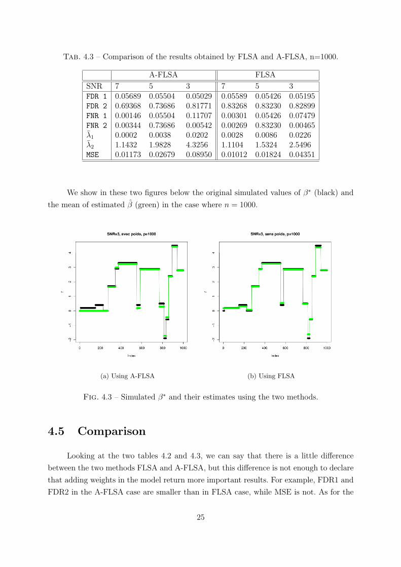
We show in these two figures below the original simulated values of β∗ (black) and

the mean of estimated β (green) in the case where n = 1000.

(a) Using A-FLSA (b) Using FLSA

Fig. 4.3 – Simulated β∗ and their estimates using the two methods.

4.5 Comparison

Looking at the two tables 4.2 and 4.3, we can say that there is a little difference

between the two methods FLSA and A-FLSA, but this difference is not enough to declare

that adding weights in the model return more important results. For example, FDR1 and

FDR2 in the A-FLSA case are smaller than in FLSA case, while MSE is not. As for the

25

FNR2, we see that sometimes is better in A-FLSA, and sometines it is not.

We always believe that A-FLSA method is better than FLSA, from theoretic point of view,

we suggest some reasons why we had not such big difference between the two methods :

– Since we are not sure about the hypotheses we need to propose about the second

term in the fused Lasso model, it is possible that we may try another criterion

than cross validation for choosing λ1 and λ2. For example, try to find a criterion

that gives the optimal value of λ1 first, then for this λ1 find the optimal λ2.

– Another suggestion is trying to adapt only the first term of the fused Lasso model,

therefore adding weights only to adapt the absolute values of the coefficients.

– Another reason we suggest is that maybe by using a bigger γ in the weights we

get a better solution, in this report we used γ = 1.

We will try to explore all these suggestions in the futur.

26

5 Conclusion and perspectives

In this report, we compared two regression/segmentation methods. We added some

weights in the well known fused Lasso regression, we called it adaptive fused Lasso. We

adapted a path algorithm that solves the fused Lasso in the case where the design matrix X

is the identity matrix and the number of observations is equal to the number of parameters

(fused Lasso signal approximator). We concluded that those weights are not so useful in

this case, they did not gave us better solutions. Probably, we are in a situation where it

is useful to adapt the Lasso penalty on the absolute values of the coefficients but no need

to adapt the Lasso penalty on the absolute value of their diffrence.

In the futur, we will investigate more about the criterion to choose the optimal values

of λ1 and λ2, we will study the suggestions that we proposed in the final comparison in

this report. From a theoretic point of view, we will investigate whether the adaptive fused

Lasso penalty has the oracle properties in the Gaussian regression context. In particular,

where we use a random matrix X as a design matrix. To do this, we will use as in [15]

some epiconvergence results of [5]. because [15] has already found some scenarios where

the Lasso does not satisty the oracle properties, while the adaptive Lasso satisfies these

properties. From the practical point of view, we will try to adapt an algorithm that solves

the fused Lasso with a random design matrix X, therefore we have to find an algorithm

in which theorem 2 holds. We also have to prove the asymptotical results of the adaptive

fused Lasso.

Finally, we will apply our algorithm on real data.

27

A Appendix

Proof of Theorem 1. We will use the same proof presented in [4]. By adding the weights

that we use in the adaptive fused Lasso, some changes will occur.

First we find the subgradient equations for β1, · · · , βn, which are

gi =∂L(y, β)

∂βi= −(yi − βi) + λ1w

(1)i Si + λ2w

(2)i Ti,i+1 − λ2w

(2)i−1Ti−1,i

where

– Si = sign(βi) if βi 6= 0

Si ∈ [−1, 1] if βi = 0, it can be chosen arbitrary (see [4]).

– Ti,j = sign(βi − βj) if βi 6= βj

Ti,j ∈ [−1, 1] if βi = βj

These equations are necessary and sufficient for the solution. As it assumed that a solution

for λ1 = 0 is known, let S(0) and T (0) denote the values of the parameters for this solution.

To be more Specific, Si(0) = sign(βi(0)) for βi(0) 6= 0. If βi(0) = 0 we choose Si(0) = 0,

since it can be chosen arbitrarily ([4]). Note that as λ2 is constant throughout the whole

proof, the dependence of β, S and T on λ2 is suppressed for notational convenience.

In order to find T (λ1), observe that soft-thresholding of β(0) does not change the

ordering of pairs βi(λ1) and βj(λ1) for those pairs for which at least one of the two is not

0 and, therefore, it is possible to define Ti,j(λ1) = Ti,j(0). If βi(λ1) = βj(λ1) = 0, then

Ti,j can be chosen arbitrarily in [-1,1] and, therefore, let Ti,j(λ1) = Ti,j(0). Thus, without

violating restrictions on Ti,j, we have T (λ1) = T (0) for all λ1 > 0. Otherwise, S(λ1) will

be chosen appropriately below so that the subgradient equations hold.

Now insert βi(λ1) = sign(βi(0)) (|βi(0)| − w(i)1 λ1)

+ into the subgradient equations.

For λ1 > 0, look at 2 cases :

28

Case 1 |βi(0)| ≥ w(i)1 λ1 ⇒ βi(λ1) = βi(0)− w(i)

1 λ1Si(0) . Then,

gi(λ1) = −yi + βi(λ1) + w(i)1 λ1Si(λ1) + w

(2)i λ2Ti,i+1 − w(2)

i−1λ2Ti−1,i

= −yi + βi(0)− w(i)1 λ1Si(0) + w

(i)1 λ1Si(λ1) + w

(2)i λ2Ti,i+1 − w(2)

i−1λ2Ti−1,i

= −yi + βi(0) + w(2)i λ2Ti,i+1 − w(2)

i−1λ2Ti−1,i = 0

by setting Si(λ1) = Si(0), and using the definition of T (λ1) and noting that β(0) was

assumed to be a solution.

Case 2 |βi(0)| < w(i)1 λ1 ⇒ βi(λ1) = 0. Then,

gi(λ1) = −yi + w(i)1 λ1Si(λ1) + w

(2)i λ2Ti,i+1 − w(2)

i−1λ2Ti−1,i

= −yi + βi(0) + w(2)i λ2Ti,i+1 − w(2)

i−1λ2Ti−1,i = 0

by setting Si(λ1) = βi(0)

w(i)1 λ1

that is ∈ [-1,1].

29

Bibliographie

[1] F. Bunea, A. Tsybakov, and M. Wegkamp. Sparsity oracle inequalities for the lasso.Electron. J. Statist., 1 :169–194, 2007.

[2] B. Efron, T. Hastie, I. Johnstone, and R. Tibshirani. Least angle regression. Ann.Stat., 32(2) :407–499, 2004.

[3] J. Fan and R. Li. Variable Selection via Nonconcave Penalized Likelihood and ItsOracle Properties. Journal of the American Statistical Association, 96 :1438–1360,2001.

[4] J. Friedman, T. Hastie, H. Hofling, and R. Tibshirani. Pathwise coordinate optimi-zation. The Annals of Applied Statistics, 1(2) :302–332, 2007.

[5] C.J. Geyer. On the asymptotics of constrained M-estimation. The Annals of Statis-tics, 22 :1993–2010, 1994.

[6] Holger Hoefling. A path algorithm for the Fused Lasso Signal Approximator. sub-mitted in October 2, 2009, 2009.

[7] M. R. Kosorok and S. Ma. Marginal asymptotics for the ”large p, small n” paradigm :With applications to microarray data. Ann. Stat., 35(4) :1456–1486, 2007.

[8] F. Rapaport, E. Barillot, and J.-P. Vert. Classification of arrayCGH data using fusedSVM. Bioinformatics, 24(13) :i375–i382, Jul 2008.

[9] S Rosset and J Zhu. Piecewise linear regularized solution paths. Ann. Statist,(35) :1012–1030, 2007.

[10] R. Tibshirani. Regression shrinkage and selection via the lasso. Journal of the RoyalStatistical Society, Series B, 58 :267–288, 1996.

[11] R. Tibshirani. The lasso method for variable selection in the Cox model. Stat. Med.,16(4) :385–395, Feb 1997.

[12] R. Tibshirani, M. Saunders, S. Rosset, J. Zhu, and K. Knight. Sparsity and smooth-ness via the fused lasso. Journal of the Royal Statistical Society Series B., 67 :91–108,2005.

[13] R. Tibshirani and P. Wang. Spatial smoothing hot spot detection for CGH datausing the fused lasso. Biostatistics, 9(9) :18–29, 2008.

[14] P. Zhao and B. Yu. On model selection consistency of lasso. J. Mach. Learn. Res.,7 :2541, 2006.

[15] H. Zou. The Adaptive Lasso and Its Oracle Properties. Journal of the AmericanStatistical Association, 101(476) :1418–1429, 2006.

30