The Baltic Dry Index: A Leading Economic

Indicator and its use in a South African context.

Dino Roberto Zuccollo

Student Number: 303144

Supervisor: Professor Kurt Sartorius

A research report submitted in partial fulfilment of the

requirements of the degree of

Master of Commerce

University of the Witwatersrand

Ethics Clearance Number: CACCN/1032

i

Table of Contents

1. Introduction ...................................................................................................... 1

1.1 Research Problem ...................................................................................... 4

1.2 Importance of the Study ............................................................................ 6

1.3 Scope and Delimitations ........................................................................... 7

2. Literature Review ............................................................................................. 8

2.1 The Mechanics of the Baltic Dry Index .................................................... 8

2.2 The Economics of the BDI ...................................................................... 13

2.2.1 Inelasticity of Supply ....................................................................... 13

2.2.2 Global Commodity Demand ............................................................ 15

2.2.3 Laycan Period and Vessel Age ........................................................ 19

2.2.4 Bunker Prices ................................................................................... 20

2.2.5 Piracy ............................................................................................... 22

2.2.6 Global Winter Severity .................................................................... 25

2.2.7 Cyclical Effects ................................................................................ 27

2.2.8 Ancillary Drivers ............................................................................. 28

2.2.9 Key Insights ..................................................................................... 28

2.2.10 Conceptual Framework .................................................................... 29

2.3 The BDI as a Predictor of Economic Activity ........................................ 30

2.3.1 Methods Employed in Other Studies ............................................... 30

2.3.2 Empirical Evidence .......................................................................... 33

2.3.3 Other Studies .................................................................................... 34

2.3.4 Forecasting Short-Term BDI Price Movements .............................. 35

2.3.5 Forecasting Long-Term BDI Price Movements .............................. 37

2.3.6 Key Insights ..................................................................................... 37

2.4 Conceptual Framework ........................................................................... 39

3. Data and Method ............................................................................................ 40

3.1 Research Question 1 ................................................................................ 40

3.2 Research Question 2 ................................................................................ 42

3.2.1 Data .................................................................................................. 42

ii

3.2.2 Method ............................................................................................ 43

3.2.2.1 Descriptive Analysis ........................................................... 43

3.2.2.2 Correlation Analysis............................................................ 45

3.2.2.3 Optimal Lag Period ............................................................. 46

3.2.2.4 ARIMA Regression ............................................................. 47

4. Findings .......................................................................................................... 49

4.1 Research Question 1 ................................................................................ 49

4.2 Research Question 2 ................................................................................ 50

4.2.1 Descriptive Analysis ....................................................................... 51

4.2.2 Correlation Analysis ....................................................................... 53

4.2.3 Optimal Lag Period ........................................................................ 54

4.2.4 ARIMA Regression ........................................................................ 56

5. Discussion of Findings ................................................................................... 58

5.1 Research Question 1 ................................................................................ 58

5.2 Research Question 2 ................................................................................ 59

5.2.1 Periods of Significant Convergence/Divergence ............................ 59

5.2.2 Correlation Analysis ....................................................................... 60

5.2.3 Optimal Lag Period ........................................................................ 62

5.2.4 ARIMA Regression ........................................................................ 63

6. Conclusion ...................................................................................................... 64

References .............................................................................................................. 66

iii

Abstract

This paper investigates the Baltic Dry Index; an often misunderstood index, which

tracks the cost of shipping dry bulk cargo globally. The research is based on the

hypothesis that movements in the Baltic Dry Index price are driven largely by

changes in the underlying demand for goods which are consumed globally.

Accordingly, this paper aims to investigate whether changes in the Baltic Dry

Index price may be used to predict future economic movements in a South

African context. In this regard, the paper first conducts a thorough synthesis of the

available literature, in order to formulate the conclusion that the Baltic Dry Index

price is driven by a multitude of variables, including the global demand for goods,

the global supply of ships, the laycan period, bunker prices, global piracy, global

winter severity, as well as the inclusion of a cyclical component. The global

demand for goods is concluded to be chief among these. Based on these findings,

the paper then conducts empirical testing on the usefulness of the BDI in a South

African context, and concludes that the Baltic Dry Index is useful when used as a

leading economic indicator in South African, especially when used in order to

predict long-term economic movements, across a period of 3 – 4.5 years. Finally,

strong evidence is found to support the existence of a relationship between the

BDI and the Johannesburg Stock Exchange Mining Index, although further

investigation is required in order to form a definitive conclusion in this regard.

1

1. Introduction

As a result of increased globalization in the 21st Century, as well as significant

reductions in transport costs, approximately 80% of world trade is currently

transported by ship, via more than 93 000 freight vessels and 1.25 million crew

members (Bowden 2010). These vessels transport an estimated 6 billion tonnes of

cargo on an annual basis; the largest proportion of which represents dry bulk

cargo1 - a category of goods which accounts for 40% of the world fleet

2 (Geman

and Smith 2012). In a South African context, the importance of dry bulk shipping

is extremely significant, with approximately 132.7 million tonnes of dry bulk

cargo having been exported by ship during 2010. This represents approximately

87% of the country’s total seaward exports for the year (South African National

Department of Transport 2011). In total, South African foreign maritime trade

comprises 3% - 4% of the aggregate tonne-miles3 of world carriage.

In order to assist the public in monitoring the cost of dry bulk shipping globally,

the Baltic Dry Index4 (BDI) is released every weekday at 13:00 by the Baltic

Exchange (Baltic Exchange 2012). The BDI tracks global shipping prices of

various forms of dry bulk cargo across twenty-five key dry bulk shipping routes,

the contracts for which are negotiated and traded on the Baltic Exchange. These

prices are obtained through the involvement of a panel of international ship-

1 Dry bulk cargo is dominated by five main commodities: iron ore, coal, phosphate, grain and

alumina (Oomen 2012). 2 The remainder of the world’s cargo fleet is comprised as follows: 38% represents tankers and

22% represents container ships (Geman and Smith 2012). 3 Investopedia (2012) defines a tonne mile as a “single ton[ne] of goods that is transported for one

mile.” 4 The Baltic Dry Index is the successor to the Baltic Freight Index and was brought into operation

for the first time on 1 November 1999 (Baltic Exchange 2012).

2

brokers, who submit dry bulk shipping prices to the Baltic Dry Exchange on a

daily basis. Figure 1 depicts the price movements of the BDI for the period April

1985 – December 2012.

Figure 1: 1985 – 2012 Baltic Dry Index Price Chart

Source: Baltic Exchange (2012)

In the short term, demand for dry bulk cargo is tight and inelastic

(Bakshi, Panayotov and Skoulakis 2010). This is due to the fact that the supply of

ships, being large and expensive capital assets, is mostly fixed in the short term.

According to Geman and Smith’s (2012) hypothetical scenario in which 100 ships

are available in order to transport 99 cargoes of grain, freight rates will remain

low due to the natural competition between shipping companies, who compete on

price in an attempt to be awarded contracts. Conversely, however, if the number

of cargoes to be transported rapidly increases to 101, freight rates will increase

3

steeply as an additional shipping vessel cannot simply be built within a few days.

As a result of this relatively constant vessel supply, changes in the aforementioned

demand, driven by increased global production and exports, directly affect the

BDI price.

This unique, price-sensitive relationship has resulted in some economic experts

using the BDI as a leading economic indicator5. Said differently, as a result of the

fact that the world freight market is a competitive environment in which the

factors of supply and demand determine the freight rate (Koskinen and Hilmola

2005), it may be possible for the BDI to be used in order to predict future stock

returns and economic activity. This is as a result of the fact that changes in the

BDI price are believed to be reflective of changes in global demand for raw

materials (Alizadeh and Talley 2010). Phillips (2010) epitomizes this viewpoint:

“And since its [the BDI’s] recent May 26 peak of 4209, the index has

dropped by nearly 55% to 1902 Friday. So, are prices in the shipping

markets signalling a hard-landing, or worse, a double dip recession?”

Blanchflower (2010: 1), too, discusses the signalling effect of the BDI. He asserts

that despite the positive economic sentiment of most investors during 2010, the

subsequent drop in the BDI “signal[led] trouble ahead”. This assertion is

strengthened by the fact that economists believe the BDI to be a pure economic

indicator which is largely devoid of speculative activity (Mowry and Pescatori

2008). According to the Baltic Exchange (2012):

5 Investopedia (2012) defines a leading economic indicator as “a measurable economic factor that

changes before the economy starts to follow a particular pattern or trend.”

4

“… it provides both a rare window into the highly opaque and diffuse

shipping market and an accurate barometer of the volume of global trade –

devoid of political and other agenda concerns.”

It is clear that the financial public perceive the BDI to be a pure and efficient

economic indicator. Despite this, the use of the BDI as a leading economic

indicator is subject to a number of complications which are yet to be resolved,

given the very limited amount of research which has been conducted on this

index. The first such issue stems from the fact that, although perceived to be a

pure economic indicator, the BDI price is nevertheless subject to a multitude of

complex external factors which may potentially impact on its price. The existing

literature has not taken cognisance of this fact and, as such, an extensive research

and synthesis of these factors in the context of the BDI, is not yet available. Until

this uncertainty is resolved, the practical application of the BDI is limited.

Previous studies have also investigated the usefulness of the BDI as a predictor

for future stock returns and economic activity in a global context, using the mean

return across a large number of territories as the data against which movements in

the BDI price have been analysed. In addition, a single study performs an analysis

of the usefulness of the BDI in an American context. No research has been

conducted on the usefulness of the BDI in a South African context, however.

1.1 Research Problem

The purpose of this research is to analyse the key factors which influence the BDI

price, as well as to assess the predictive properties of the BDI in a South African

context. In light of the aforementioned relationship between the BDI and the

5

demand for goods which are exported globally, it is hypothesized that the BDI and

its sub-indices may be used in order to predict stock price movements and

economic activity in a South African context. This is coupled with the fact that the

export of goods must intuitively precede their ultimate sale. In order to investigate

this relationship, the following two research questions are established:

1. Research Question 1 (RQ1): Which factors influence movements in the

BDI price?

2. Research Question 2 (RQ2): Can the BDI be used as a predictor for South

African stock price movements and economic growth?

In order to use the BDI as a predictor for future economic activity, it is

fundamental that the factors which drive the BDI price are extensively researched

and understood as per RQ1. If the BDI is to be used as a leading economic

indicator, it must first be proved that a change in the demand for dry bulk cargo is

a key factor influencing the BDI price. In lieu of this, a flawed perception of the

mechanics of the index may result in the BDI being used to predict future

economic activity, when in fact the BDI price is being driven by factors which are

not indicative of changes in the underlying demand for dry bulk cargo. It is

hypothesised that these additional price drivers will be found exist as a result of

the fact that even the most pure economic indicators are driven by a multitude of

factors in the complex arena of business in the 21st Century (Geman and Smith

2012). Despite this, a thorough investigation of all factors which influence the

BDI price will allow the potential investor to first identify whether global demand

for goods is a key BDI price driver and second to understand that any potential

6

change in the BDI price must also be interpreted in conjunction with an

understanding of changes in other factors which may influence the BDI price.

Upon gaining a more thorough understanding of the factors which drive the BDI

price, RQ2 will then explore the possibility of using the BDI and its sub-indices as

a predictor for future South African stock returns and economic activity. In

addition, the information obtained in RQ1 will empower the potential investor to

isolate demand-driven movements in the BDI price from movements driven by

non-demand related factors.

1.2 Importance of the Study

This study is of importance as very little research has been performed regarding

the predictive properties of the BDI, with no research having been conducted in a

South African context. As a result of the fact that dry bulk cargo carriers account

for 40% of the world fleet of transport vessels (Geman and Smith 2012), the

economic significance of the BDI price is immense. A conclusion which supports

the research hypothesis, that the BDI may be used as a leading economic indicator

in a South African context, would unearth a previously unknown and little-

respected economic forecasting tool. The practical implications thereof would be

extensive: for example, potential investors would be better equipped to make

decisions relating to investment opportunities, company executives could make

more informed strategic business decisions and those involved in the formulation

of monetary policy would be able to formulate better inflation and economic

growth forecasts, to name but a few.

7

In addition, this paper may serve as a platform for future studies which seek to

investigate the usefulness of the BDI. Such studies may include, but are not

limited to, research into those issues specifically excluded from the scope of this

paper in terms of the Scope and Delimitations section, as well as the issues

identified in the Findings section of this paper.

1.3 Scope and Delimitations

This research will investigate the applicability of the BDI in a South African

context only. The possibility of its use in other global territories does not form

part of the scope of this paper, although an extension of the methods employed in

this paper across other global territories is identified as a possibility for future

research. In addition, this paper does not attempt to formulate a new model to

predict the BDI, although a number of existing models are cited in the Literature

Review, below.

RQ1 is focused on identifying the fundamental BDI price drivers only. It is noted

that there are likely to be a multitude of ancillary factors which drive the BDI

price which will not be discussed in this research. As a result of the fact that these

ancillary factors are not likely to be fundamental to changes in the BDI price, they

are immaterial in relation to the research conducted and are therefore not

considered. In addition, this research does not aim to develop a model in which

the potential impact of non-demand related BDI price drivers are removed in

order to develop a more pure BDI price. This is as a result of the fact that many

fundamental BDI drivers are of a non-discrete nature and can therefore not be

8

quantified numerically. The existence of global piracy, which is discussed in more

detail in the Literature Review, below, is one such example.

As regards the research pertaining to RQ2, it is noted that his study is of an

exploratory nature only. As such, a full empirical investigation of the relationship

between a lagged BDI and all JSE sectors is outside the scope of this paper, but is

identified as a potential topic for future research. In addition, in interpreting the

findings of RQ2, it is noted that economic activity is a function of many factors

which are not limited to the BDI price alone. These factors, however, are not

relevant to this research as it is only the relationship between the BDI and

economic activity which falls within the scope of this paper.

2. Literature Review

The literature review investigates the economics of the BDI and its subsequent

linkages to economic activity. In addition, in order to present the data necessary in

order to answer RQ1, the first section of this review will conduct an extensive

analysis and synthesis of the available literature in order to identify the

fundamental factors which drive the BDI price. Despite the fact that the Scope and

Delimitations section has made reference to the fact that it is not practically

possible to identify all factors which result in variations in the BDI price, it is

nevertheless hypothesized that the fundamental BDI price drivers may be

unearthed through the analysis below.

2.1 The Mechanics of the Baltic Dry Index

The Baltic Exchange can be traced back to 1744, where it derives its name from

the coffee house Virginia and Baltick; a restaurant which was frequented by

9

British residents in order to negotiate agreements for the transportation of goods

by ship (Baltic Exchange 2012). Although only formalized in later years, the

Baltic Exchange established its first committee of 23 shipping merchants in 1823

and subsequently registered as a primitive form of a company in 1857. Today,

membership comprises 600 companies and more than 3 000 individuals, rendering

the Baltic Exchange the most important market for shipping, and the only

independent source of maritime information, in the world (Wall Street Journal

2007; Geman and Smith 2012). The most recent addition to the Baltic Exchange is

the Baltic International Freight Futures Exchange (BIFFEX), which was

established at the Baltic Exchange’s headquarters in London, England, in 1985.

The Baltic Exchange also operates out of a regional office in Singapore.

In addition to the release of the BDI, the Baltic Exchange also provides additional

useful information to investors by dividing the overall BDI into four sub-indices,

namely the Capesize (BCI), Panamax (BPI), Supramax (BSI) and Handysize

(BHSI) indices (Baltic Exchange 2012). These sub-indices reflect the cost of

shipping items of differing sizes, with the dead weight in tonnes that the ships are

capable of transporting forming the basis for this classification. Figures 2 and 3,

below, provide additional information regarding these classifications and the price

histories thereof. The overall BDI is then calculated as the weighted average cost

of carriage of dry bulk cargo across these four indices, multiplied by a

predetermined factor. This multiplier factor was first introduced when the BDI

replaced the Baltic Freight Index in 1999 and is used in order to standardise the

BDI price due to frequent amendments to the BDI contributing indices, as well as

10

to the method of BDI calculation. Mathematically, the formula used for the

creation of the BDI may be expressed as:

(CapesizeTCavg + PanamaxTCavg + SupramaxTCavg + HandysizeTCavg) / 4 *

0.113473601

Where TCavg = Time charter average.

Source: Baltic Exchange (2012)

Figure 2: Composition of the BDI

Dead Weight in

Tonnes

Percentage of

World Fleet

Percentage of Dry

Bulk Traffic

Capesize Index 100 000+ 10% 62%

Panamax Index 60 000 – 80 000 19% 20%

Supramax Index 45 000 – 59 000 37% 18%*

Handysize Index 15 000 – 35 000 34% 18%*

* Represents a percentage within the respective index

Source: Shriram Insight (2009); Geman and Smith (2012)

The routes tracked by each BDI sub-index are detailed in Figure 4, below. Each

sub-index monitors the cost of carriage of dry bulk goods across 4-9 global

shipping routes (Baltic Exchange 2012). These routes vary in both length and

geographic locality in order to ensure that the sample of shipping costs tracked by

the BDI and its sub-indices are reflective of the global cost of shipping. The route

prices are then weighted by the importance of the route in the dry bulk sector and

summed in order to obtain the BDI sub-index price, which is reported daily

(Geman and Smith 2012).

11

Figure 3: BDI Sub-Index Price History

Source: Baltic Exchange (2012)

Of particular relevance to this research is route C4, which is tracked by the overall

BDI, and more specifically the Capesize Index. The cost of shipping a 150 000

metric tonne vessel between Richards Bay in South Africa and Rotterdam in the

Netherlands is tracked and weighted at the 5% level when calculating the

Capesize Index price (Baltic Exchange 2012). The port of Richards Bay is South

Africa’s premier bulk port and operates through a dry bulk terminal, a coal

terminal and a multipurpose terminal (Ports and Ships 2012). In 2011/2, the port

handled 89.232 million tonnes of cargo. This port is connected to South Africa via

a series of dedicated rail networks which ensure efficient carriage to and from the

country’s central economic hubs. This indicates that the BDI price is directly

influenced by South African import/export data. Despite the fact that the

12

aforementioned relationship is not a pre-requisite for this research, it is

nevertheless useful in highlighting the applicability of the BDI price in a South

African economic context.

Figure 4: BDI Sub-Index Routes

Route

Number

Route Description Weighting

Capesize Index

C2 160 000lt Tubarao – Rotterdam 10%

C3 160 000mt or 170 000mt Tubarao – Qingdao 15%

C4 150 000mt Richards Bay – Rotterdam 5%

C5 160 000mt or 170000mt West Australia – Qingdao 15%

C7 150 000mt Bolivar – Rotterdam 5%

C8 03 172 000mt Gibraltar/Hamburg Trans-Atlantic 10%

C9 03 172 000mt Continent/Mediterranean Trip 5%

C10 03 1720 00mt Pacific 20%

C11 03 172 000mt China/Japan Trip 15%

Panamax Index

P1A 03 74 000mt Transatlantic 25%

P2A 03 74 000mt SKAW – GIB/Far East 25%

P3A 03 74 000mt Japan – SK/Pacific 25%

P4 03 74 000mt Far East/NOPAC – Australia 25%

Supramax Index

S1A Antwerp – Skaw Trip Far East 12.5%

S1B Canakkale Trip Far East 12.5%

S2 Japan – SK / NOPAC or Australia 25%

S3 Japan – SK Trip 25%

S4A US Gulf – Skaw-Passero 12.5%

S4B Skaw-Passero – US Gulf 12.5%

Handysize Index

HS1 Recalada – Rio de Janeiro 12.5%

HS2 Boston – Galveston 12.5%

HS3 Rio de Janeiro Trip Skaw – Passero. 12.5%

HS4 US Gulf trip via US Gulf or NCSA to Skaw – Passero 12.5%

HS5 South East Asia trip via Australia to Singapore – Japan 25%

HS6 S Korea – Japan via NOPAC to Singapore – Japan 25%

Mt = Metric Tonne Lt = Litre

Source: Baltic Exchange (2012)

13

2.2 The Economics of the BDI

2.2.1 Inelasticity of Supply

In order for the hypothesis of this paper to hold true, it must be proved that the

supply of ships is tight and inelastic in the short-term. To this end, Bakshi,

Panayotov and Skoulakis (2010: 4) detail how the high costs and significant lead

times involved in new ship acquisitions results in a situation where the “supply

structure of the shipping industry is generally predictable and relatively inflexible

[over a short-term horizon].” Devanney (2010) agrees with this, by explaining that

the short-run container ship supply function is simply the horizontal sum of the

global fleet’s tonne-mile capacity. Said differently, the short-run supply function

of cargo vessels is limited to the capacity of the current global fleet, owing to the

fact that additional vessels cannot be constructed in the short-run.

The capital-intensive task of manufacturing a new cargo ship can take two to three

years complete; a time frame which is far longer than the short-term fluctuations

experienced on the demand-side of cargo carriage (Koskinen and Hilmola 2005;

Wall Street Journal 2007). A 75.9 metre, second-hand container ship, for example,

currently retails for approximately USD 5 900 000 (Maritime Sales Inc. 2012); a

sizeable investment which cannot simply be entered into on an ad-hoc basis. As a

result, ship-owners tend to order new ships during periods when global demand is

strong and receive them a number of years later, where a real possibility exists

that both demand and freight rates may have weakened.

High costs are not the only factor leading to the relatively stable supply of the

global cargo fleet, however. Koskinen and Hilmola (2005) explain that the

14

uncertain profitability expectations associated with ownership of expensive cargo

ships, coupled with the aforementioned lengthy ship manufacturing process, leads

to a situation in which would-be ship-owners seek to rather lease freight vessels as

opposed to obtaining the outright ownership thereof. This, they conclude, creates

a situation in which the supply of cargo ships is relatively stable. Matthews (2003)

provides an example of the effect of this stable ship supply on the BDI price, by

detailing how the BDI price doubled during the two months ended October 2003

as a result of the fact that surging Chinese demand for freight vessels far

outstripped supply at the time. A similar situation occurred a few years later,

when freight rates tripled between 2006 and 2007. This was as a result of the

rapidly expanding economic growth in developing economies such as China and

India (Matthews 2007). This growth had the effect of increasing the BDI price by

169% over the same time period. The fact that the supply of ships remained

relatively stable during the economic growth of both 2003 and 2007, demonstrates

that the demand-side of the BDI drives its price in the short-term, due to the stable

supply of ships. As a result, the global fleet supply is not identified as a

fundamental BDI price driver in the short-run.

According to the Baltic Exchange (2012), in the long-term, the number of

different types of ships available globally, as well as the quantity of these ships

which are currently in operation, is a variable which influences the BDI price.

Tvedt (2003) explores the characteristics of this influencing factor further, by

using the augmented Dickey-Fuller test in order to evidence that long-term freight

rates are mean-reverting in nature. He attributes this tendency to the behaviour of

ship-owners: when demand increases, so too do freight rates as a result of the

15

constant short-term ship supply detailed above. In order to cope with this

increased demand, ship-owners construct new vessels and also devise methods in

order to utilize their existing capacity more efficiently. As a result, long-term ship

supply is increased and the originally elevated freight rates consequently begin to

revert to their mean levels. Similarly, lower freight rates prompt ship-owners to

scrap costly vessels, thereby increasing freight rates to similar levels. Due to this

phenomenon, the nature of the global supply of ships has the impact of creating a

mean-reverting tendency in freight rates over the long-term.

2.2.2 Global Commodity Demand

In order to uncover the drivers of the BDI price, the Baltic Exchange (2012)

identifies a number of variables. They explain that while the BDI is driven by a

large range of external factors, there are a number of fundamental drivers which

underpin all BDI price changes. The first, and most fundamental of these drivers

is the demand for commodities, which the Baltic Exchange identifies as being

influenced by issues such as the global level of industrial production, the quality

of crop harvests, global industry performance, power usage, etc. Figure 5, below,

evidences this link graphically, by plotting the annual growth in the world Gross

Domestic Product6 (GDP) against the growth in global exports across an

equivalent time period. It is clear that growth in the global GDP has the effect of

increasing the number of goods which are exported, with the opposite holding true

for a decline in the global GDP.

6 Gross Domestic Product is a term which denotes the total monetary value of all finished goods

and services which are produced within a territory for a given period of time, normally measured

in years. This figure is calculated by determining the sum of all private and public consumption,

investments and exports and subtracting from this the value of any imports made into that territory

across the same time frame (Investopedia 2012).

16

Figure 5: Growth Rate of Global Exports Plotted Against Global GDP Growth

Rates

Source: Oxford Economics (2007)

The literature above has established that the global supply of ships is relatively

stable in the short-run, rendering the BDI a demand-driven index. As such, an

increase in the level of goods exported globally, as per Figure 5, will have the

effect of increasing the BDI price (Oxford Economics 2007). This provides proof

that changes in commodity demand is a fundamental BDI price driver.

Another example of the relationship between the BDI price and the demand for

commodities is the case of China. According to Hyung-geun (2011), many believe

the Chinese to be a G2 nation; an unheralded economic force without which

global trade would suffer. The impact which China has on the world economy is

17

so strong, he argues, that many have begun to refer to this contribution as the

China effect. This can be demonstrated through the 500% growth in Chinese

exports from $249.2 billion in 2000, to roughly $1.3 trillion in 2009. On the basis

of this premise, Hyung-geun tests the relationship between the BDI price and the

Chinese demand for commodities by performing an event study analysis pre and

post the decision by the Chinese government to ban new investment in industries

such as steel, automobiles and real estate. The subsequent decrease in demand

post the implementation of the ban resulted in a BDI price reduction of

approximately 38% in less than two months. This is a clear demonstration of the

so-called China effect and what has become known as the China shock; the

sudden and significant drop in price which changes in Chinese production cause

on the shipping industry and, in turn, the BDI price. As such, it may further be

concluded that demand is a fundamental BDI price driver in a Chinese context.

Changes in the BDI price have also been linked to changes in economic activity in

various other world economies. In a British context, Oxford Economics (2009)

detail the significant impact that the United Kingdom shipping industry has on the

British GDP. The report outlines how the British shipping industry supports

212 000 jobs in total, and directly contributes a turnover of £9.8 billion to the

British GDP. The indirect impact of the shipping industry on the British economy

is even more significant, with ship-manufacturers, rail companies, port service

providers, advertisers, etc. all deriving a large proportion of their revenues from

the shipping industry. Oxford Economics also attribute the BDI’s climb from

$3177 in 2006, to $7071 in 2007, to strong demand for iron ore in emerging-

markets’ steel industries. Furthermore, their paper predicts that the contraction of

18

the British GDP in the last two quarters of 2008 would have the effect of creating

a slowdown in the United Kingdom shipping industry. This proved true, as is

evidenced by the severe decline in the BDI price during 2008 and 2009, as per

Figure 1, above. This is a clear indication that, in a British context, there is a

strong link between economic activity and shipping prices, as reflected by the

BDI price.

Radelet and Sachs (1998) build on the understanding of the link between

economic output and the shipping industry, by evidencing a statistically

significant link between a country’s proximity to a harbour and its economic

growth rate. It is for this reason, he argues, that the Mediterranean basin, which is

serviced by many navigable rivers, has grown at a far more rapid pace than inland

Africa, which enjoys no such access to waterways. Inland economies, such as

Mongolia and Rwanda, are proven to exhibit far lower GDP growth rates when

compared to their coastal counterparts, such as the United States and the United

Kingdom. Within the top 15 export growth economies during the period 1965 –

1990, almost the entire population lived within 100km of the coast, compared to

the in-sample proportion of 45% on the total sample tested. Even if these

landlocked territories were to cut tariff rates, remove restrictions on trade and

implement more prudent macroeconomic policies in order to stimulate trade, they

would still not be able to compete with their coastal competitors. This is as a

result of the fact that the high transport costs incurred by these territories would

render their products more expensive than similar goods which are produced

along the coast. Inland territories pay between 25% and 288% more for inter-

19

modal7 export shipments, despite the fact that the inland transport component of

the goods shipped comprises only a small proportion of the total distance

travelled. In order to remain competitive, these businesses would have no choice

but to decrease wages, thereby stagnating economic growth within the inland

economy.

2.2.3 Laycan Period and Vessel Age

Having explored the impact of commodity demand on the BDI price, it is

necessary to research the potential impacts of other drivers on the BDI price. To

this end, Alziadeh and Talley (2010) use an Ordinary Least Squares regression

model in order to test the relationship between the BDI price and a list of

predefined variables. They conclude that in both the Capesize and Panamax

markets, the laycan period8, as well as the size of the transport vessels used, is

statistically significant when regressed against the BDI price.

The intuitive hypothesis that as ships grows older, they grow more expensive to

operate, is also proved true as a result of the negative and nonlinear relationship

which is evidenced between vessel ages and their respective hire rates (Alziadeh

and Talley 2010). In addition, it is determined that a longer laycan period is

associated with higher freight rates. This, Alziadeh and Talley explain, is as a

result of the actions taken by ship-charters when a shortage in ship supply is

anticipated. As global economic activity increases, so too does the demand for

7 Inter-modal transport refers to goods which must travel by both land and sea in order to reach

their destination (Radelet and Sachs 1998). 8 The laycan period is jargon specific to the shipping industry (Alziadeh and Talley 2010) and

denotes the period of time between the fixture date and the layday. The fixture date is defined as

the date of the conclusion of negotiations between the ship-owner and ship-charterer. The product

of these negotiations is a signed charter contract. The layday is defined as the contractually

stipulated date on which the chartered ship must be delivered to the charterer.

20

freight vessels. Under these conditions, ship-charterers become more inclined to

hire vessels earlier in order reduce the possibility of future unavailability in cargo

capacity. This tendency both lengthens the laycan period and increases the cost of

freight, indicating not only that the BDI price is driven by the length of the laycan

period, but also indirectly evidencing the link between global economic output

and the BDI price.

2.2.4 Bunker Prices

Bunker prices9 account for approximately 25% - 33% of the total cost of operating

a transport vessel (Baltic Exchange 2012). As a result of the fact that bunker

prices are closely related to crude oil prices, the extremely volatile movements in

the oil price directly affect ship owners and, in turn, the BDI price (Notteboom

and Vernimmen 2008; Geman and Smith 2012). Figure 6, below, depicts the

movements in the crude oil price during the period 2008 – 2012. The large decline

in the oil price during the six months ended December 2008 is of particular

importance, as this decline of approximately 57% took place during the same

period in which the BDI price, depicted graphically in Figure 1, above, tumbled.

Although it may be argued that both of these price movements are largely

attributable to the 2008 Global Financial Crisis, it is nevertheless clear that oil

prices have a significant impact on the BDI price.

9 The Oxford Dictionary (2012) defines a bunker as “a large container or compartment for storing

fuel.” For a detailed description on the production methods of bunker fuel, see Notteboom and

Vernimmen (2008).

21

Figure 6: 2008 – 2012 Crude Oil Price

Source: NASDAQ (2013)

The aforementioned relationship is empirically tested in the literature, via a

various number of studies: Notteboom and Vernimmen (2008) explain that a

major factor considered by ship-owners when deciding where to dock their ships

is the relative price of bunker fuel across available ports, which differs as a result

of varying fiscal policies and fuel taxes between countries. The nature of these

varied and volatile bunker costs leads to a situation in which charterers tend to

deliver cargo on time only when bunker costs are borne by the charterer. In this

situation, the cost of fuel is irrelevant to ship operators. When ship-owners are

required to absorb the increased costs associated with volatile fuel price swings,

however, the proportion of on-time charters reduces. This is as a result of a variety

of cost-cutting measures which ship-owners implement in order to offset the

impact of higher bunker prices. These measures normally include the conservation

22

of fuel through the implementation of decreased vessel speeds, coupled with the

addition of new ships to supply routes.

The impact of bunker prices on freight rates has resulted in the advent of a global

shipping convention in which freight rates are quoted exclusive of a Bunker

Adjustment Factor (BAF); an adjustment factor which is added to freight rates on

a monthly basis in order to account for variations in bunker prices (Notteboom

and Vernimmen 2008). This factor was introduced in 1974 as a response to the

first oil crisis, and effectively protects ship-operators’ net profits by shifting the

impact of changes in bunker prices from the ship owner, to the ship charter

(Notteboom and Cariou 2009).

The application of this factor is not perfect, however, as it has been empirically

proven that a $1 change in bunker prices has the impact of changing the BAF by

approximately $1.5. This would indicate that the BAF amplifies the impact which

changes in bunker prices have on freight rates (Cariou and Wolff 2006). The

impact of this is not only to create a strong link between bunker prices and freight

rates (Devanney 2010), but also between bunker prices and the BDI price. It can

therefore be concluded that bunker prices are a fundamental BDI price driver.

2.2.5 Piracy

The existence of choke points in global shipping routes is identified as another

key factor driving the BDI price (Fu, Ng and Lau 2010). Nearly half of the

world’s oil tankers pass through a handful of narrow sea corridors, which are

often subject to terrorist attack, conflict, severe winters and accidents as a result of

high traffic volumes (Baltic Exchange 2012). Should any of these incidents occur,

23

the corrective or evasive actions required by shipping companies would adversely

affect the world’s supply patterns; a cost which is ultimately borne by the final

consumer.

In recent times, piracy in areas such as the Somali coastline, the Gulf of Aden and

the Suez Canal has become the most significant consequence of the existence of

these choke points. According to Bowden (2010), approximately 500 seafarers

from more than 18 countries were held hostage by pirates around the globe at the

end of 2010. Although difficult to quantify, Bowden estimates that piracy costs

the global economy between $7 billion and $12 billion per year. In November

2010, a ransom of $9.5 million was paid to Somali pirates in order to ensure the

safe release of the Samho Dream, a South Korean oil tanker. The magnitude of

this ransom, the highest ever recorded, highlights the rapid increase in global

piracy; the average ransom demanded by pirates has increased from $150 000 in

2005, to a predicted $5.4 million in 2010.

Despite the significant economic impact of the ransoms charged by pirates, the

indirect costs of piracy have been far more significant. International insurance

companies have been forced to increase premiums in order to cope with the

increased risk premiums associated with the carriage of cargoes by sea (Bowden

2010). War risk insurance premiums10

, for example, have increased from $500 per

voyage in 2008, to as much as $150 000 per voyage in 2010. In addition, kidnap

and ransom insurance has increased 10 fold between 2008 and 2009, whilst hull

insurance has doubled over a similar period. For some cargo operators, these

10

War risk insurance premiums are charged when cargo vessels pass through areas considered

‘war risk areas’ by global insurance companies (Bowden 2010).

24

increased premiums, when considered with the potential human fatalities

associated with incidents of piracy, have rendered travel through the Gulf of Aden

and the Suez Canal unfeasible. As a result, many cargo operators have decided to

re-route South, past the Cape of Good Hope – a diversion which adds 3500 miles

to the voyage of most cargo vessels (Gilpin 2009). Although the exact quantity of

ship-operators who have decided to amend their cargo routes is not ascertainable,

Fu, Ng and Lau (2010) develop a model which estimates that 18% of shipping

companies would elect this diversion11

in the absence of governmental efforts to

curb piracy. It is estimated that this diversion costs the shipping industry between

$2.3 and $3 billion per annum, whilst the lost revenues in the countries which had

serviced the old shipping routes, amounts to an anticipated $30 million.

Furthermore, the need to install deterrent equipment, employ on-board security

personnel, contribute towards anti-piracy organizations and prosecute those

responsible for incidents of piracy, all contribute to the costs borne by freight

companies (Bowden 2010). The Yemeni Navy, for example, charges as much as

$60 800 per cargo vessel in order to ensure safe passage through the Gulf of Aden

(Kraska 2010). Should significant measures not be put in place in order to curb

international piracy, the potential also exists for the piracy incidence rate to

increase in the future. This is as a result of the fear that other terrorist cells, such

as Al Shebab12

, may partner with existing pirates in an attempt to further

11

Fu, Ng and Lau (2010) estimate that a total of 30% of shipping companies would elect some

form of a diversion, however. 12

Al Shebab is the biggest militant organization fighting against the transitional government in

Somalia, although the group has become active in other territories, such as Uganda, in recent times

(Stanford 2013).

25

destabilise the region (Gilpin 2009). Figure 7, below, plots the global incidents of

piracy reported during the period 2006 – 201213

.

Figure 7: 2006 – 2012 Global Incidents of Piracy

Source: Statista (2012)

2.2.6 Global Winter Severity

The length and severity of ice winters along key shipping routes, coupled with

seasonal pressures such as reduced global crop yields during the winter months

which would otherwise have required shipping, is identified as a further BDI price

driver (Baltic Exchange 2012). These pressures are especially significant along

the choke points outlined in the paragraphs above: although located in a warm and

humid climate along the mid-latitudes, the Baltic Sea experiences severe ice

13

At the time of writing this paper, the total statistics for 2012 had not yet been gathered due to

delays in the collation and transmission of piracy incidence data.

26

winters, especially between January and March each year (Hagen and Feistel

2005).

Koslowski and Loewe (1994) investigate variations in the extent of winter ice

cover over the Baltic Sea. The research shows that weak to moderate ice winters

prevail, occurring 75.4% of the time, whilst very strong ice winters occur 24.6%

of the time. This research indicates that approximately one in every four Baltic

winter is likely to adversely affect ship operators along the route; a significant

figure in light of the high volumes of traffic passing through the Baltic region on

an annual basis.

The 2002/3 winter in the Gulf of Finland, which borders the Baltic Sea, was an

example of a particularly severe ice winter which asked a number of questions as

to the suitability of world freight vessels in coping with particularly demanding

ice conditions (Koskinen and Hilmola 2005). During the period, the icy winter

conditions lead to a number of tanker accidents and oil spills along to Gulf, which

endangered not only the marine ecology within the immediate vicinity of the

accidents, but also the ability of freight companies to transport cargo during the

winter season. So frequent and severe was the prevalence of these accidents that

the European Union has recently taken measures to prevent a large portion of the

world’s older and potentially substandard tanker fleet from loading and unloading

oil in European Union harbours. This legislation has the effect of reducing the

amount of freight vessels which are capable of servicing much of Europe, thereby

reducing ship supply and impacting the BDI price. This indicates that the length

and severity of global winters plays a role in the determination of the BDI price.

27

2.2.7 Cyclical Effects

In addition to the drivers identified above, Goulielmos and Psifia (2006) show that

freight rates possess a 2.25 to 4.5 year cyclical tendency; a finding which is

logically re-enforced by the fact that both the recessions of the 1970s and of the

1990s lasted approximately 5 years. The mean reverting nature of freight rates,

discussed above, adds credence to this argument (Tvedt 2003). If it is understood

that freight rates tend to diverge from their mean value, and then revert back to

that value at some point in the future, it can be argued that this property is in itself

is a form of cyclicality, provided that the length of the reversion property is

constant. In the case of freight rates, this is proven true through the findings of

Goulielmos and Psifia.

Koskinen and Hilmola (2005) further evidence the cyclical property of freight

rates, by explaining how both supply and demand-related factors create cyclicality

in the global freight market. On the demand side, freight prices are inextricably

linked to the world economy, in which an increase in people’s mean living

standard results in an increased demand for transportation. As such, the natural

cyclicality between periods of economic growth and recession in the global

economy creates a similar characteristic in shipping prices. On the supply side, the

major contributing factor is the tendency of ship-owners to overestimate their

forecasts of economic growth during periods of expansion. As a result, ship

owners order too many new vessels, which are subject to long lead times, and

create an oversupply of cargo ships post the peak in freight demand upon eventual

receipt.

28

2.2.8 Ancillary Drivers

Other ancillary BDI price drivers are also identified in the literature, although

most authors concede that these factors are not fundamental BDI price

determinants. An example of such a driver is the quality of port administration

and infrastructure; the more efficient the port authority, the less bureaucratic red

tape and customs clearance corruption is encountered when shipping, thereby

lowering freight prices (Radelet and Sachs 1998). In addition to this, more

efficient ports are also likely to charge lower handling fees, thereby increasing the

significance of their relationship to freight rates.

Other ancillary drivers include political factors, average haul and currency value

fluctuations (Oomen 2012). Measures implemented by governments in order to

promote local production and sales, for example, may reduce the BDI price

without being indicative of a reduction in underlying economic activity. The same

is true for shipping costs which are denominated in a foreign currency and are

subject to the volatile movements in forex prices. Despite the existence of these

ancillary drivers, they are not identified as being fundamental to the determination

of the BDI price and are therefore not considered further in this research.

2.2.9 Key Insights

The first phase of this research has conducted an extensive synthesis of the

available literature in order to gain a better understanding of the mechanics of the

BDI, as well as to identify a number of key variables which underpin movements

in the BDI price. As evidenced by the Baltic Exchange (2012), the BDI is a well-

established index, which provides an accurate reflection of the price of shipping

29

globally. The BDI price is also relevant in a South African context, due to the fact

that the cost of shipping goods along the Richards Bay – Rotterdam route is

included in the calculation of the overall BDI price. This fact, when considered in

conjunction with the finding that the global ship supply is relatively stable in the

short-term, leads to the conclusion that the BDI would appear to be useful as an

economic tool in a South African context, provided that the remainder of the

research hypothesis is empirically proven in the literature.

Thereafter, further investigation of the literature reveals that the global demand

for shipping is a fundamental BDI price driver, although other ancillary price

drivers are also evident which may distort the perceived impact of demand on the

BDI price. These ancillary drivers include the laycan period, the average vessel

age, bunker prices, the existence of choke points along global shipping routes,

piracy and the length and severity of winters along key shipping routes. Shipping

prices have also been shown to possess a cyclical tendency, across periods of

between 2.25 and 4.5 years.

Finally, the literature does identify other ancillary BDI price drivers, such as

evidenced in the work of Radelet and Sachs (1998) and Oomen (2012). Despite

the existence thereof, these drivers are not identified as being fundamental BDI

price drivers and are therefore outside of the scope of this paper.

2.2.10 Conceptual Framework

The identification of these factors allows for the formulation of the first element

of the Conceptual Framework, on which the remainder of the research will be

based:

30

RQ1

Figure 8: Conceptual Framework I

2.3 The BDI as a Predictor of Economic Activity

The next component of this research aims to analyse the literature pertaining to

the use of the BDI as a predictor of economic activity in a global context. In this

regard, the work of Bakshi, Panayotov and Skoulakis (2010) and Oomen (2012) is

identified as the two key research papers on the topic. Despite the fact that these

papers are useful in gaining an understanding of the predictive powers of the BDI

in a global context, neither paper performs any meaningful investigation into the

factors which drive movements in the BDI price. It is as a result of this that this

paper aims to overcome these shortcomings through the detailed investigation

performed above.

2.3.1 Methods Employed in Other Studies

The first of the aforementioned papers to be published is the work of Bakshi,

Panayotov and Skoulakis (2010). The aim of their research is to investigate

whether the BDI price has predictive ability when compared to a range of global

BDI price driven, in large,

by the global demand for

commodities and other

dry bulk goods

Overall BDI:

Comprising

o Capesize,

o Panamax

o Supramax

o Handysize

sub-indices.

Other BDI Price Drivers:

o Ship supply (relevant

in the long-run only)

o Laycan period length

o Vessel size and age

o Bunker prices

o Piracy

o Length and severity

of global winters

o Cyclicality

31

stock markets and commodity prices. In order to investigate this, Bakshi,

Panayotov and Skoulakis make use of the out-of-sample R² statistic of Campbell

and Thompson (2008), as well as an in-sample inference, based on the

conservative Hodrick (1992) covariance estimator. The market data against which

the BDI is tested is obtained from four MSCI14

regional stock market indices, as

well as from the individual stock markets of all of the G-7 countries. In addition,

stock market data from 12 developing countries is included in order to avoid a

developed-economy bias. The small number of developing countries used in the

testing is attributed to a lack of sufficiently reliable stock market return data in

territories other than the 12 cited in the paper. It is worth noting that South Africa

forms one of the developing economies included in the research. Despite this,

however, the study does not provide a vast quantity of quantifiable data as to the

usefulness of BDI as a predictor in a South African context, as a result of the fact

that Bakshi, Panayotov and Skoulakis do not perform their regression analyses on

a country-by-country basis, but rather on a broader level of aggregation, which

includes all countries which form a part of the MSCI, as well as the developing

countries selected. As such, the findings of the study draw a conclusion on the

relationship between the BDI and the global economy only, and not on a territory-

specific basis.

In order to develop a point-estimate of the performance of the BDI, against which

the MSCI stock returns may be tested, Bakshi, Panayotov and Skoulakis (2010)

use a lagged, three month BDI growth rate, although this lag period is neither

tested, nor justified by the authors. As such, the abstract selection of a lag period

14

Metals Service Centre Institute

32

for the purposes of the testing is identified as a shortcoming which the Data and

Method section of this paper will seek to overcome.

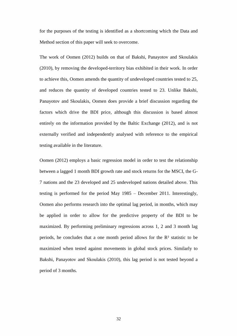
The work of Oomen (2012) builds on that of Bakshi, Panayotov and Skoulakis

(2010), by removing the developed-territory bias exhibited in their work. In order

to achieve this, Oomen amends the quantity of undeveloped countries tested to 25,

and reduces the quantity of developed countries tested to 23. Unlike Bakshi,

Panayotov and Skoulakis, Oomen does provide a brief discussion regarding the

factors which drive the BDI price, although this discussion is based almost

entirely on the information provided by the Baltic Exchange (2012), and is not

externally verified and independently analysed with reference to the empirical

testing available in the literature.

Oomen (2012) employs a basic regression model in order to test the relationship

between a lagged 1 month BDI growth rate and stock returns for the MSCI, the G-

7 nations and the 23 developed and 25 undeveloped nations detailed above. This

testing is performed for the period May 1985 – December 2011. Interestingly,

Oomen also performs research into the optimal lag period, in months, which may

be applied in order to allow for the predictive property of the BDI to be

maximized. By performing preliminary regressions across 1, 2 and 3 month lag

periods, he concludes that a one month period allows for the R² statistic to be

maximized when tested against movements in global stock prices. Similarly to

Bakshi, Panayotov and Skoulakis (2010), this lag period is not tested beyond a

period of 3 months.

33

2.3.2 Empirical Evidence

Upon completion of their testing, Bakshi, Panayotov and Skoulakis (2010) are

able to conclude that an increase in the BDI growth rate is associated with higher

future stock returns across a one month time horizon, especially in the Industrial

sector. This they prove through the findings of in and out-of-sample testing which

indicates that 8 out of the 11 regional indices tested show p-values of below 0.05.

In addition, the adjusted R²’s of between 1.9% and 3.8% indicate weak levels of

correlation, when compared to the findings of other predictive regressions which

have been performed using estimators other than the BDI in the past. The

exception to this is the Japanese stock market, which appears to fluctuate

relatively independently of movements in the BDI price. When testing whether

the other methods of stock price estimation are more effective than the BDI price,

the research indicates that the lagged 3 month BDI growth rate outperforms both

the lagged MSCI World Index return and the lagged US return, when applied as

predictors for global stock returns, although a potential lag period in excess of 3

months is not considered.

Oomen (2012) finds that a 1 month lagged BDI growth rate shows positive α2

coefficients for the countries tested, indicating that the BDI returns have a positive

effect on global stock markets. More specifically, an increase in the BDI return of

one standard deviation, or 16.2%, is found to result in an increase of 0.78% in the

MSCI World Index return. This relationship is further enhanced when controlling

for the impact of the oil price on the BDI return, as a result of fact that the largest

percentage of operational costs borne by ship-owners are incurred on purchasing

fuel; a price driver which is not linked to the global demand for commodities. In

34

addition, when analysing the predictive properties of an oil-corrected BDI in the

context of 10 industry-specific sectors, it is found that the BDI is most effective as

a predictor for global stock returns in the Technology, Telecommunications,

Consumer Services and Industrial sectors. The BDI Panamax Index is also shown

to be the best predictor of economic activity, although no explanation is provided

as to the possible reasons for this.

Finally, Oomen (2012) finds that the BDI can only be concluded to be an accurate

predictor of global stock returns for the period 2001-2007 in developed countries,

and for the periods 2001-2007 and 2008-2011 in undeveloped countries. This, he

hypothesises, may be as a result of the fact that an economic boom was only

experienced during the period 2001-2007 in developed countries, prior to the

global financial crisis. As such, it may be possible that the BDI is reliant on

periods of economic growth and stability in order to serve as a predictor for global

economic activity and stock returns. The validity of this finding in a South

African context will be tested further in Data and Method section of this paper,

below.

2.3.3 Other Studies

Other papers which evidence the predictive property of the BDI are also

identified, including the work of Ou-Yang, Wei and Zhang (2009), who agree

with the findings of Bakshi, Panayotov and Skoulakis (2010), by concluding that

the BDI has predictive power in an American context. In addition, Kärrlander and

Lanneström (2010) uncover a statistically significant correlation between the BDI

and the MSCI Metals & Mining index. Mariana (2008), too, uses mathematical

35

models in order to conclude that steel and corn prices show the strongest

correlation to the BDI growth rate. This indicates that the BDI can be used to

forecast movements in the value of these commodity indices, albeit that the

research is conducted in a non-South African context.

2.3.4 Forecasting Short-Term BDI Price Movements

It is submitted that this research paper is neither concerned with the methods by

which the BDI can be forecast, nor on identifying which of these methods is most

effective. A brief discussion on these models is nevertheless provided as a result

of the fact that this paper would have very little practical application should it not

be possible to forecast movements in the BDI price.

Duru (2010) develops a Fuzzy integrated logical forecasting model in order to

forecast short-term movements in the BDI. He argues that previous attempts at

BDI forecasting models have been accurate only insofar as they are capable of

predicting a particular type of data in an academic sense. The use of these models

in forecasting an index, which is affected by a range of variables and data sets, has

little use in a practical environment. Duru explains how, as a result thereof,

statistical extrapolation using these models leads to inconsistent results and the

need to apply judgemental forecasting. This is inappropriate in a mathematical

model which, by definition, is based purely on data and is devoid of all subjective

human inputs. To this end, Duru’s Fuzzy Integrated Logical Forecasting Model

provides superior accuracy than classical time series methods due to the

incorporation of an error correction function and a white noise15

reduction feature.

15

The Concise Oxford English Dictionary (2002) defines white noise as “noise containing many

frequencies with equal intensities”. From a mathematical standpoint, however, this definition is

36

Duru concludes that his model may be used to accurately predict future BDI

movements.

Chou (2008) applies Chou and Lee’s Fuzzy Time Series Model to predict the BDI

for the forthcoming month. This forecast is generated, plotted graphically in

Figure 9, below, and compared to actual BDI movements for the given time

period. The root-mean-squared-errors are then calculated and used to assess the

significance of BDI forecasting errors, from which Chou is able to conclude that

Chou and Lee’s Fuzzy Time Series Model is suitable for the BDI’s prediction.

Figure 9 – Real and Forecast BDI using Chou and Lee’s Fuzzy Time Series

Model

adapted to refer to a means by which data involving sudden and extremely large fluctuations is

normalized.

37

The mathematical work of Duru (2010) and Chou (2008) is countered by that of

Tsakonas, Nikolaidis and Dounias (ca. 2000), who apply a self-learning fuzzy

prediction system to forecast short-term movements in the BDI Panamax

category. They conclude that, although their prediction model is reliable, there is

“no substitute [for] the analytical mind of a human being” (Tsakonas et al ca.

2000:9). As such, they argue that a mixture of fundamental analysis and

mathematical models is most effective in determining future movements in the

BDI.

2.3.5 Forecasting Long-Term BDI Price Movements

Whilst the literature above is focused mainly on predicting short term BDI

movements, Fang (2007) develops a mathematical model to be used by investors

in order to hedge out longer-term risks inherent in the BDI. He uses Fractal

Theory to effectively predict the long-term memory property of the BDI

Handymax, Panamax and Capesize categories, as well as the volatility of returns.

The BDI Panamax category is found to exhibit the strongest long-term memory

property, although all three categories tested display significant long-term

memory properties. As such, the BDI is capable of being predicted in both the

long and short terms, making it a viable tool in predicting future economic activity

in a South African context.

2.3.6 Key Insights

As is apparent from the discussion above, very little work has been performed

regarding the usefulness of the BDI in predicting future stock returns and

economic activity. In this regard, only two previous studies are identified as

38

having researched this topic in detail, albeit that neither thereof provides any

meaningful analysis of the factors which influence movements in the BDI price,

prior to the commencement of testing. The first such paper is that of Bakshi,

Panayotov and Skoulakis (2010), which concludes that the BDI is useful as a

predictor of stock returns in a global context. This finding is in agreement with the

work of Oomen (2012), which represents the second significant paper identified

on the topic. Oomen does qualify his findings, however, by indicating that the

BDI has exhibited a period of significant convergence against the world returns

tested, for the period 2001 – 2007/8, after which a period of significant divergence

was evidenced from 2008/9 – 2011. Furthermore, it is proven that the BDI serves

as an effective predictor in an American context (Ou-Yang, Wei and Zhang 2009).

Despite the fact that Bakshi, Panayotov and Skoulakis’ work includes South

African economic performance within the aggregate pool of data tested, none of

the abovementioned studies are identified as providing any form of information

regarding the applicability of the BDI in a South African context.

Upon testing the sectors which exhibit the highest degree of correlation to the BDI

price, Bakshi, Panayotov and Skoulakis (2010) conclude that the BDI is most

effective as a predictor in the Industrial sector. Oomen (2012) agrees with this, but

adds that the BDI also serves as an effective predictor in the global Technology,

Telecommunications and Consumer Services sectors. Furthermore, the work of

Kärrlander and Lanneström (2010) evidences that the BDI is also effective as a

predictor outside of a stock market context, by proving statistically significant

levels of correlation between the BDI price and the prices of both corn and steel.

39

The literature then assesses the optimal lag period to be applied to the BDI price

in order to maximize the degree of correlation against the global returns analysed.

Bakshi, Panayotov and Skoulakis (2010) conclude that a 3 month lag period is

most appropriate, whilst Oomen (2012) concludes that a shorter 1 month period

results in the maximization of the BDI predictive property. Neither of these papers

tests a lag period of beyond 6 months, however.

Finally, it is concluded that the BDI price is capable of prediction over both short

and long-term periods. In this regard, Duru (2010) and Chou (2008) outline

effective short-term prediction models, whilst Fang (2007) indicates that the use

of Fractal Theory yields positive long-term prediction results. Despite these

positive findings, it is noted that a combination of both mathematical models, as

well as the application of an analytical human mind, often yields the most

accurate prediction results (Tsakonas et al ca. 2000).

2.4 Conceptual Framework

Having outlined the literature pertaining to RQ2, the Conceptual Framework

developed in Figure 8, above, may be extended in order to outline the interaction

between RQ1, RQ2 and the literature discussed. This Conceptual Framework will

underpin the remainder of the research to be performed, and is presented in Figure

10, below:

40

RQ2

RQ1

Figure 10: Conceptual Framework II

3. Data and Method

The Data and Method section outlines the particulars of the method applied in

order to meet the Research Objectives, outlined above. It also details the data

inputs used in order to perform this research, along with the necessary internal and

external validity testing which is required in order to assess the appropriateness of

the research findings.

3.1 Research Question 1

As has been indicated in the Literature Review, this study employs a mixed-

methods approach in order to answer Research Question 1: which factors

influence movements in the BDI price? This is due to the large quantity of

complex factors which influence the BDI price, and the subsequent influence of

these factors on economic activity (Ryan and Scapens 2002). Furthermore,

Underlying Economic

Activity:

o BDI effective as a

predictor in a global

context

o Periods of significant

convergence and

divergence

o Correlation

maximized when

tested against

certain sectors

o Optimal lag period

of between 1 and 3

months

o BDI capable of

prediction

BDI price driven, in large,

by the global demand for

commodities and other

dry bulk goods

Overall BDI:

Comprising

o Capesize,

o Panamax

o Supramax

o Handysize

sub-indices.

Other BDI Price Drivers:

o Ship supply (relevant

in the long-run only)

o Laycan period length

o Vessel size and age

o Bunker prices

o Piracy

o Length and severity

of global winters

o Cyclicality

41

Contents Analysis (Creswell and Piano 2007) has been employed in order to

identify consistent themes and patterns in the literature.

In this regard, the validity of findings has been ensured through the inclusion of

research which has been obtained from reputable sources only. These sources

include journal articles, theses published by recognized educational institutions,

conference papers and information obtained directly from the subjects of the

research, such as the Baltic Exchange (2012). The validity of findings has been

further ensured by comparing the results of the papers discussed above with the

large quantity of other research available on the respective topics. This has been

performed in order to ensure that the findings thereof are logical and in line with

the arguments presented in this paper. In the rare circumstances in which

discrepancies have been noted, these papers have been either removed from the

analysis provided, or the disagreements between the various articles have been

highlighted and explained in order to caution the reader against drawing

conclusions from papers in which consensus has not yet been reached. The

determination of the most appropriate course of action in the abovementioned

circumstances has been made depending on the significance of the disagreement

identified. In addition, an indication of the rigour of the testing performed within

these papers has been provided, in order to ensure that it is only the findings of the

most comprehensive research which are relied upon.

This analysis has led to the creation of a single, focused set of empirically tested

data, which may be used in support of the definitive identification of the

fundamental BDI price drivers. Mathematically, the first Research Question is

formulated as:

42

BDI = f(X1 + X2 + X3 + … Xi)

Where X = factors influencing the BDI price.

Through the development of the conceptual framework understanding of the

factors which drive the BDI price, the extensive Literature Review conducted

allows for the quantification of the proposed solution to this Research Question,

without the performance of additional empirical testing. These research findings

are detailed in the Findings section, below.

3.2 Research Question 2

The second phase of this research will comprise the empirical testing of the

relationship between the BDI and the South African economy, in order to resolve

Research Question 2: can the BDI be used as a predictor for South African stock

price movements and economic growth? As such, it must be proven that South

African share or commodity prices are a function of the BDI price, should it be

concluded that the BDI may be used as a leading economic indicator in a South

African context. For the purposes of the empirical testing, this objective is

formulated mathematically, as:

Share Price/Commodity Price = f(BDI)

3.2.1 Data

The Reuters (2013) website is utilized in order to access the BDI price data to be

used as the independent variable input in the testing, below. According to

Thomson Reuters (2013), the company is the “leading source of intelligent

information for the world’s business professionals” and operate out of more than

43

100 countries worldwide, reported 2012 revenues of $12.9 Billion and enjoy a

staff compliment of more than 60 000 employees. As such, the BDI price data

extracted may be accepted as being accurate and complete, as it has been obtained

from a reputable source.

The Johannesburg Stock Exchange (JSE) Index data established as the dependent

variable in the testing performed is extracted from the McGregor Bureau for

Financial Analysis (2013) website. McGregor has featured as a leading South

African market-data provider since its origin in 1965, and is well respected in the

industry. As such, the information obtained from this source is accepted as

accurate.

Monthly BDI and JSE Index returns have been extracted for the period

01/04/1997 - 31/01/2013 for all testing performed. Due to the large number of

correlation tests performed, this 15 year period is argued to be sufficient for the

purposes of the analysis. In addition, the 191 observations collected are sufficient

in order to allow for the creation of a reliable moving average for the purposes of

the ARIMA regression model run.

3.2.2 Method

A four-stage approach is adopted in order to conduct the testing per RQ2. Each of

these stages is outlined in detail below:

3.2.2.1 Descriptive Analysis

The first stage of testing comprises a descriptive analysis, with the aim of

evidencing a prima facie relationship between the BDI and the JSE All Share

44

Index (ALSI), from a visual perspective. In order to perform this analysis, the

ALSI will be used as a proxy for the performance of the South African market at

large. It is argued that the ALSI serves as a suitable measure of the performance

of the South African economy as a whole, as the Index tracks the weighted

average performance of all shares listed on the JSE (JSE 2013). This argument is

supported by the fact that the 368 companies listed on the JSE enjoyed a

combined 2012 pre-tax profit of R760 billion (JSE 2012). In addition, the JSE

ranks as one of the Top 20 exchanges in the world in terms of market

capitalization. Given the magnitude of the JSE in a South African context, it is

reasonable to rely on the mean return of the shares contained therein as an

accurate measure of South African economic activity.

This prima facie analysis is performed by plotting monthly movements in both the

BDI price and the JSE ALSI price graphically, in order to assess the relationship

between the two variables from a visual perspective. It is intended that this initial

phase of research will allow for the potential relationship between both variables

to be assessed visually, prior to the commencement of the mathematical

regression analysis. In addition, a cyclic filter will be applied to the data

presented, in order to remove any ‘white noise’ contained therein. This will

provide further insight into the relationship between the two. In addition, it is

hypothesised that the smoothed data plot will assist in the commencement of the

remaining phases of empirical testing, namely the correlation analysis, the

quantification of the optimal lag period between the BDI and South African stock

market returns and the BDI/ALSI regression analysis. It is important to note that,

should this initial phase of testing not indicate the possibility of a relationship

45

between these variables, the continuance of additional testing would likely not

support a conclusion in favour of the research objective.

3.2.2.2 Correlation Analysis

The second stage of testing comprises an extensive correlation analysis between

the BDI and a number of preselected JSE Indices, with the objective of identifying

the indices which exhibit the greatest correlation to the BDI. For the purposes of

this testing, the correlation coefficient, or R², between a non-lagged BDI and the

various JSE Indices is calculated in terms of the following equation:

Where

SSyy = Deviation from the mean

SSE = Deviation between observations and their predicted values.

The JSE Indices selected for testing can be classified into three batches, based on

the rationalization for selection: the first batch tested comprises the JSE All Share,

Top 40, Mid Cap and Small Cap Indices, which are tested in order to examine the

relationship between the BDI and entities of various sizes within the South

African economy. Thereafter, the second batch of testing comprises a the testing

of the correlation between the BDI and the South African Mining Index, based on

the fact that the Rotterdam – Richards Bay route is included within the BDI price

46

calculation, as detailed earlier in this paper16

. Thereafter, the third and final batch

is selected based on the combined findings of Bakshi, Panayotov and Skoulakis

(2010) and Oomen (2012), who find that the Technology, Telecommunications,

Consumer Services, Industrial and Food Producers Indices exhibit the strongest

correlation to the BDI. The indices regressed are summarised in Figure 11, below:

Figure 11: Indices Selected for Correlation Analysis

Index Analysed JSE Code Reason Selected for Testing

All-Share Index J203 To assess the overall relationship between the

BDI and the South African economy

Top 40 J200 To determine whether the BDI exhibits a

statistically stronger relationship when regressed

against entities of a particular size

Mid-Cap J201

Small Cap J202

Mining J177 To determine whether the magnitude of the

mining sector within the South African economy,

as well as the inclusion of a South African route

within the BDI price calculation, results in a

stronger correlation between the BDI and the

South African Mining Industry.

Technology J590

To test the findings of Oomen (2012), in a South

African context

Telecommunications J560

Consumer Services J550

Industrials J520

Food Producers J357

3.2.2.3 Optimal Lag Period

Post the completion of the correlation analysis, the third phase of empirical testing

is conducted in order to assess the practicality of potential investors and other

market participants being able to use the BDI as a leading economic indicator. As

explained in the Introduction to this paper, in order for the BDI to be useful,

movements in the BDI price must be proven to precede movements in the South

16

Due to the fact that the largest percentage of cargo handled by the Richards Bay harbour

represents dry bulk cargo which is exported by the South African Mining Industry, as well as the

fact that 70% of the world’s coal exports originate from South Africa, Australia and North

America collectively (Tvedt 2003), it is hypothesized that a significant correlation may exist when

assessing the relationship between the BDI and the South African Mining Index.

47

African economy. In order to assess this, the BDI price will be lagged and tested

against the ALSI, as well as the Index which exhibits the strongest correlation

against the BDI, in order to determine the lag period, in months, which maximizes

the correlation coefficients between the two. Should this optimal period be found

to be a lag period, it may be concluded that the BDI is useful when applied as a

leading economic indicator.

3.2.2.4 ARIMA Regression

The fourth and final stage of testing comprises the application of an Auto-

Regressive Integrated Moving Average (ARIMA) analysis, in order to prove that

a causal relationship exists between the BDI and the South African market as a

whole. Such a finding is necessary in order to enhance the usefulness of the

findings of the correlation analysis, which is only capable of indicating the

existence of a relationship between variables, and not the existence of causal

relationship between the two. In order to perform this regression, the overall BDI

price is constructed as the model independent variable, and the JSE ALSI is

established as the dependent variable. The ALSI has been selected for the purpose

of this testing, as a result of the fact that it represents the best indicator of

aggregate economic activity in South Africa.

The ARIMA model is selected due to the fact that it is able to account for non-

stationarity in data (Duke University 2013). As such, the model accounts for the

fact that both the BDI and the ALSI exhibit a trend over time. Should these trends

not be incorporated in the regression model run, the existence thereof may lead to

48

misleading findings regarding causality. In addition, an ARIMA17

model accounts

for autocorrelation, through the Portmanteau Q-Statistic Test. As such, the model

assists in ensuring the validity of findings through the elimination of potentially

misleading research findings which arise through the analysis of variables which

exhibit serial autocorrelation.

The ARIMA model applied is quantified as:

In order to ensure the validity and reliability of findings, the Portmanteau Q-

Statistic is calculated in order to test for autocorrelation in the data input. In

addition, a T-Statistic test is performed in order to evidence that the variance

against zero is one-sided, thus indicating that the relationship between the BDI as

the independent variable, and the ALSI as the dependent variable, is positive and

that the direction of the relationship is consistent with the objective of the paper.

As a result of the fact that the Z-Statistic test is often criticised as being simple in

its nature, a more rigorous, two-sided Chi-Square test will then be performed at a

95% confidence interval, in order to evidence a causal relationship between the

dependent and independent variables tested.

17

For a more detailed outline of the mechanics of the ARIMA regression model used, the reader is

directed to the work of Tseng, Tzeng, Yu and Yuan (2001).

49

As stated in the Scope and Delimitations section, it is important to note that this

regression analysis is only performed with the objective of proving a causal

relationship between the BDI and the ALSI, in order to enhance the findings of

the correlation testing. As such, it is only the relationship between the ALSI and a

non-lagged BDI which is tested. The testing of the ALSI against a lagged BDI is

outside the scope of this paper, but is identified as a potential for future research.

4. Findings

4.1 Research Question 1

The extensive review of the literature above indicates that the BDI price is driven

by a multitude of factors. These factors are summarized in Figure 12, below:

Figure 12: BDI Price Drivers

BDI price driven, in large,

by the global demand for

commodities and other

dry bulk goods

Overall BDI:

Comprising

o Capesize,

o Panamax

o Supramax

o Handysize

sub-indices.

Other BDI Price Drivers:

o Ship supply (relevant

in the long-run only)

o Laycan period length

o Vessel size and age

o Bunker prices

o Piracy

o Length and severity

of global winters

o Cyclicality

50

Mathematically, this relationship may be quantified as:

BDI = f(underlying economic activity, ship supply, laycan period length,

vessel size and age, bunker prices, global maritime piracy, global winter

severity, cyclicality, error term)

The literature has presented a clear set of BDI price drivers, with very little

contradiction having been evidenced amongst the articles identified. Furthermore,

upon analysis of additional papers in order to evidence the validity of findings, the

research conclusions were found to be logical and consistent with the large

quantity of additional articles consulted.

The most common theme across the articles analysed is that of the relationship

between the BDI price and the demand for shipping. This leads to the conclusion

that demand is a fundamental BDI price driver. Despite this, the additional drivers

identified also exhibit a material impact on the BDI price. It is further noted that

the significance of each of these drivers is likely to change in the future, as the

nature of global trade evolves. For this reason, secondary data has been extracted,

where possible, in order to provide a measure by which the prevalence of each of

these drivers may be analysed. The crude oil price and the number of incidences

of global piracy, per Figures 6 and 7, above, are two such examples. The

Literature Review, above, provides a full analysis of all secondary data extracted.

4.2 Research Question 2

The testing of the relationship between the BDI and the South African economy

yields a number of significant findings. The first thereof is that the descriptive

analysis indicates that the BDI and the ALSI have exhibited a clear graphical

51

relationship for the period 01/04/1997 – 31/01/2013, especially when the impact

of any ‘white noise’ in the data is removed. In addition, the BDI price exhibits a

high degree of correlation between 6 of the 10 JSE Indices tested, with the

positive correlation coefficient values exceeding 0.33 for all 6 of these indices.

The highest correlation coefficient is exhibited between the BDI and the JSE

Mining Index, with a value of 0.5125. Upon lagging the BDI price against these

Index returns, the BDI/Mining Index correlation coefficient is maximized at a lag

period of 36 months, whereas the correlation between the ALSI and a lagged BDI

is maximized at a period of 54 months. Finally, the ARIMA regression indicates a

significant causal relationship between the BDI and the ALSI, with no significant

autocorrelation exhibited in the model residuals. These findings are further

enhanced through the model validity tests performed, which support the

conclusions drawn.

Sections 4.2.1 – 4.2.4, below, provide further detail with respect to the findings of

the research conducted. Thereafter, Section 5 provides a detailed discussion of

these findings.

4.2.1 Descriptive Analysis

Figure 13, below, depicts the relationship between monthly BDI price and JSE

All-Share Index price movements for the period 01/04/1997 - 31/01/2013. When

this relationship is depicted graphically, it becomes apparent that the BDI and the

ALSI have exhibited similar trends for the 1997 – 2011, after which they have

diverged significantly.

52

Figure 13: BDI/ALSI Price Chart

In order to further assess this relationship, the ‘white noise’ contained within the

data above has been eliminated by smoothing the returns through the use of a

cyclic filter, in Figure 14, below. This smoothed plot provides a clear indication of

the fact that the BDI and the ALSI are correlated. In addition, an analysis of the

graphical results would suggest that there is a lag between the BDI and the ALSI,

with movements in the BDI price clearly preceding movements in the ALSI. The

question remains, however, as to what the degree of correlation is exhibited

between the two, as well as what lag period that maximizes the degree of the

abovementioned correlation.

01

00

00

200

00

300

00

400

00

AL

SI (J

20

3)

0

500

01

00

00

150

00

BD

I O

ve

rall

1/1/1997 1/1/2001 1/1/2005 1/1/2009 1/1/2013Date

BDI Overall ALSI (J203)

53

Figure 14: BDI/ALSI Smoothed Price Chart

4.2.2 Correlation Analysis

The correlation analysis performed at a zero lag period reveals a statistically

significant degree of correlation between the BDI and a large number of the JSE

Indices tested. A summary of these findings is depicted in Figure 15, below.

Interestingly, the testing reveals that the degree of correlation between the BDI

and the dependent variables tested is maximized when the BDI price is regressed

against the JSE Mining Index, which exhibits a correlation coefficient of 0.5125.

54

Figure 15: BDI/JSE Index Correlation Coefficients

4.2.3 Optimal Lag Period

In order to perform the third phase of analysis, a further examination of the degree

of correlation between a lagged BDI and the ALSI, as well as a lagged BDI and

the Mining Index, is performed. As such, a lag period of 1 – 96 months was

applied to the BDI price, in order to determine the period, in months, in which the

degree of correlation between the BDI and these indices, is maximized. The

findings of this analysis are depicted in Figure 16, below.

55

Figure 16: BDI/ALSI and BDI/Mining Lagged Correlation Coefficients

At a zero month lag period, the correlation between the BDI and the Mining Index

is greater than between the BDI and the ALSI. Both degrees of correlation

decrease slightly at a lag period of 12 months. Thereafter, the degrees of

correlation begin to increase steeply as the lag is extended. The correlation

between the BDI and the Mining Index is maximized at a lag period of 36 months,

at which the correlation coefficient peaks at a correlation of close to 0.7.

Thereafter, this correlation declines steeply to a correlation of only 0.2 at 96

months. In contrast, the BDI/ALSI correlation coefficient continues to increase

beyond the 36 month lag, and is maximized at period of 54 months, where the

correlation peaks at a similar level of approximately 0.7. Thereafter, the

56

correlation begins to drop to a value of 0.6 at a 96 month lag, at which point the

analysis ceased.

4.2.4 ARIMA Regression

The ARIMA18

regression results are detailed in Figure 17, below:

Figure 17: ARIMA Regression Results

18

The ARIMA regression has been performed using Stata Version 10, with ARIMA Specification

(1, 1, 1): ARMA Lags AR1, MA1 and MA4.

57

The regression indicates a significant causal relationship between the BDI and the

ALSI, with Z = 8.66 and P>|z| = 0.000, when

∑

∑

There are still high levels of autocorrelation with respect to the first difference, as

denoted by AR(L1), as well as for the first moving average, as denoted by

MA(L1). This significant autocorrelation is not evidenced in the fourth difference

of moving average MA(L4), however. In its entirety, the ARIMA model has

accounted for autocorrelation, as indicated by the Portmanteau Q-Statistic in

Figure 18, below, which shows Prob>chi2 = 0.4476. This indicates that no

significant autocorrelation exists in the model residuals.

Figure 18: Portmanteau Test

The Z-Statistic test of variance against zero is found to be one sided, thereby

evidencing the validity of the finding that the BDI, as the independent variable, is

the factor driving movements in the Indices tested. This finding is further

enhanced through the conclusion that the more rigorous, two-sided Chi-Square

test is truncated at zero, at a 95% confidence level. As such, the validity of the

causal relationship between the BDI price and the Indices tested is proven.

58

5. Discussion of Findings

5.1 Research Question 1

As hypothesized at the beginning of this paper, it is found that the BDI price is a

product of a large number of variables, which are not confined to the global

demand for commodities alone. Despite this, the conclusion that demand is a

fundamental BDI price driver, allows for the creation of the theoretical foundation

from which the analysis of the second research question may be performed.

The relevance of the determination of the BDI price drivers is crucial in

interpreting the conclusions of this paper; whilst the findings of RQ2 may

conclude that the BDI is effective as a leading economic indicator, it must be

understood that changes in the BDI price are not driven by changes in the demand

for commodities alone. As such, a change in the BDI price must be analysed in

conjunction with the relevant information pertaining to the ancillary BDI price

drivers identified. These include the global supply of ships, the laycan period,

vessel size, bunker prices, global piracy, weather patterns and the consideration of

an overall cyclical component. This is not to imply that, should global bunker

prices increase, for example, a change in the BDI price is not useful as a leading

economic indicator. Rather, should such a scenario occur, it is likely that a change

in the BDI price will be less useful than what it would have been, should this have

not occurred.

In light of the above, a discussion of the findings regarding the empirical testing

pertaining to RQ2 is now presented.

59

5.2 Research Question 2

5.2.1 Periods of Significant Convergence/Divergence

On initial inspection of the graphical relationship between the BDI and the ALSI,

it is immediately clear that there exists some form of a relationship between the

BDI and the South African stock market. This is further enhanced through the

application of the cyclic filter, which indicates that the hypothesized predictive

power of the BDI appears to hold true. Interestingly, the relationship between the

BDI and the overall South African economy exhibits a period of significant

convergence between 1997 and 2011, and a period of significant divergence

during 2011 and January 2013. This finding is consistent with that of Oomen

(2012) and is highlighted in Figure 19, below.

Although this paper is not focused on unearthing the reasons for this recent

mismatch, it is nevertheless identified as a potential cause for concern for South

African investors and other market participants. A possible explanation for this

recent divergence is that the measures implemented by the South African

government in order to boost the economy post the 2008 Global Financial Crisis,

may have resulted in the economically unfeasible position in which the South

African market has been boosted through an artificial injection of both capital and

investor optimism. Contrary to this, the current BDI price indicates an economy in

which trade activity is relatively low and devoid of economic growth. It is

important to note, however, that this paper has not tested this hypothesis, although

this is identified as a potential for future research.

60

Figure 19: BDI/ALSI Divergence

5.2.2 Correlation Analysis

On performance of the correlation testing, it is found that, at a lag period of zero

months, the monthly BDI returns show the most significant correlation to the JSE

Mining Index. This result is of significance, as it is contrary to the finding of

Bakshi, Panayotov and Skoulakis (2010), that the BDI exhibits the strongest

correlation to the global Industrial sector. This is testament to the fact that the

South African economy differs to the world economy in the sense that it is driven,

in large, by the Mining Industry, which in turn uses local harbours to export the

largest percentage of ore extracted during the mining process.

One such harbour is the Port of Richards Bay, in which the largest percentage of

cargo handled represents dry bulk cargo exported by the South African Mining

01

00

00

200

00

300

00

400

00

AL

SI (J

20

3)

0

500

01

00

00

150

00

BD

I O

ve

rall

1/1/1997 1/1/2001 1/1/2005 1/1/2009 1/1/2013Date

BDI Overall ALSI (J203)

61

Industry (Ports and Ships 2012). As discussed earlier, the Richards Bay -

Rotterdam route is one of the routes tracked in the formulation of the BDI price.

Given this, along with the fact that 70% of the world’s coal exports originate from

South Africa, Australia and North America collectively (Tvedt 2003), the

significant correlation between the BDI and the South African Mining Industry is

logically re-enforced.

When regressed against the ALSI, the BDI exhibits a correlation coefficient of

0.3412, indicating that a strong relationship exists between the BDI and the South

African economy as a whole. In addition, this finding indicates that it may be

possible to use the BDI in order to predict future economic movements and stock

prices. This is discussed further in Section 5.2.3, below.

It is also found that the BDI price exhibits a strong correlation to the Top 40,

Small Cap, Telecommunications and Industrial Indices, with a BDI correlation in

excess of 0.33 for all of four of these sectors. As such, the finding of Oomen

(2012) that the BDI exhibits a statistically significant relationship when regressed

against the Telecommunications and Industrial Indices, is upheld in a South

African context. Despite this, no evidence is found in support of the conclusion

that the BDI is also an effective predictor of movements in the Technology and

Consumer Services Indices. It is also noted that, despite the strong relationship

exhibited between the BDI and the JSE Small-Cap Index, the relationship appears

less strong when analysed against the Mid-Cap Index.

62

5.2.3 Optimal Lag Period

The unearthing of a strong correlation between the BDI and both the ALSI, as

well as the Mining Index, is not in itself sufficient evidence in order to conclude

that the BDI is an effective leading economic indicator. A critical element of a

leading economic indicator is that it must also possess a predictive property; the

lag factor evidenced in the testing performed has proven this. As a result of the

finding that the correlation coefficient between the BDI and the ALSI/Mining

Index is increased as returns in these Indices are lagged, it becomes apparent that

the BDI exhibits the essential properties of a leading economic indicator.

Interestingly, the BDI lag period which maximizes the abovementioned

correlation coefficients appears higher than initially hypothesized, at 3 years when

regressed against the ALSI, and 4.5 years when regressed against the Mining

Index. This is also contrary to the findings of Bakshi, Panayotov and Skoulakis

(2010), as well as of Oomen (2012), who both conclude that far shorter lag

periods, of 3 months and 1 month respectively, maximize this correlation. It is

submitted, however, that neither of these analyses considered the potential of a

longer-term lag period. As such, the conclusions drawn from these papers are not

directly comparable against the findings of this research.

As per the discussion above, the research findings indicate that although the BDI

is useful as a leading economic indicator when used as a short-term predictor, it is

most effective when used over a longer-term period. An argument in support of

this finding is that it is consistent with the nature of the Indices tested; both the

BDI and the JSE Indices analysed comprise a measure of trade data across a large

63

quantity of companies. As such, the mean performance thereof is unlikely to differ

significantly over a short-term period, although this becomes relevant across a

longer-term period of analysis. As such, changes in the BDI price are better

equipped to measure longer-term economic movements, although a less accurate

short-term predictive property is nevertheless maintained.

Despite this potential justification, the magnitude of the discrepancy between the

optimal lag period identified in a South African context, and those identified in a

global context per previous studies, indicates the need for further research

pertaining to the optimal BDI lag period. As identified in the Scope and

Delimitations section, this paper comprises an exploratory study of the usefulness

of the BDI in a South African context. As such, a full empirical investigation of

the relationship between a lagged BDI and all available South African sectors is

outside the scope of this paper, and is identified as a possible topic of future

research.

5.2.4 ARIMA Regression

It is important to note that the findings discussed above are based predominantly

on the strength of the evidence obtained from the conducting of numerous

correlation analyses. Although the analysis of the correlation between two

variables is useful in highlighting the relationship between the two, it does not

necessarily indicate that this is a causal relationship. As such, the ARIMA

regression between the BDI and the ALSI, as a proxy for the overall South

African economy, is very significant as a result of the fact that it evidences that a

64

change in the BDI price causes a corresponding change in the ALSI price. This

finding of causality adds strength to the abovementioned findings.

This is further enhanced through the model validity tests performed, which

confirm both the internal and external validity of findings. As a result of the fact

that the possibility of autocorrelation in the data input has been disproven,

coupled with the fact that the relationship between the BDI and the Indices tested

has been validated, it is reasonable to rely on the research findings as being

consistent with the conclusions drawn.

6. Conclusion

This paper has conducted a thorough analysis of the BDI and its usefulness as a

leading economic indicator in a South African context. In this regard, an extensive

review and synthesis of the available literature has been performed, as well as the

conducting of empirical testing on the topic. In the course of this research, a

number of findings have been identified, from which the following conclusions

may be drawn:

First, although many believe the BDI price to be a pure economic indicator, it is

nevertheless driven by a number of underlying variables. These variables include,

but are not limited to, the global demand for commodities, the global supply of

ships, the laycan period, bunker prices, piracy, global winter severity, as well as

the inclusion of a cyclical component. Despite the identification of these price

drivers, the exact impact of each of these variables on the BDI price is not reliably

quantifiable. It is further concluded that the fundamental BDI price driver is

represented by the global demand for commodities.

65

Second, strong evidence is obtained in order to support the conclusion that the

BDI is effective when used as a leading economic indicator in a South African

context, although its usefulness varies depending on the JSE market sector

analysed. This conclusion is further enhanced by the findings of the ARIMA

regression analysis, which indicates that a significant causal relationship exists

between the BDI and the ALSI. In addition, the BDI exhibits the highest

correlation to the JSE Mining Index, although significant relationships are also

identified between the BDI and the JSE ALSI, Top 40, Small-Cap, Technology

and Industrial Indices. It is also concluded that the BDI appears most effective

when used as a leading economic indicator in the long-term, with an associated

lag period of between 3 and 4.5 years, depending on the JSE sector analysed.

Finally, investors and potential market participants are cautioned that the current

divergence between the BDI price and the JSE ALSI may suggest a future

economic downturn in the South African economy. The reasons for this

divergence, along with a full investigation of the relationship between a lagged

BDI, its lagged sub-indices19

and all available JSE Indices, are further identified

as possibilities for future investigation and research.

19

As outlined earlier in this paper, the BDI sub-indices comprise the Baltic Capesize, Panamax,

Supramax and Handysize Indices.

66

References

Alziadeh, A. and Talley, W. (2010) Microeconomic determinants of dry bulk

shipping freight rates and contract times, Transportation, vol. 38, pp. 561-

579.

Bakshi, G. Panayotov, G. and Skoulakis, G. (2010), The Baltic Dry Index as a

Predictor of Global Stock Returns, Commodity Returns, and Global

Economic Activity.

Baltic Exchange, About Us, last accessed on 26 December 2012, from

http://www.balticexchange.com

Blanchflower, D. (2010) The Baltic Dry signals trouble ahead, New Statesman,

vol. 139 (5012), pp. 17.

Bowden, A. (2010) The Economic Costs of Maritime Piracy, Working Paper, One

Earth Future Foundation.

Campbell, J. and Thompson, S. (2008) Predicting excess stock returns out of

sample: Can anything beat the historical average?, Review of Financial

Studies, vol.21, pp. 1509-1531.

Cariou, P. and Wolff, F. (2006) An analysis of bunker adjustment factors and

freight rates in the Europe/Far East market (2000-2004), Maritime

Economics and Logistics, vol.8(2), pp. 187-201.

Chou, M. (2008) A Fuzzy Time Series Model to Forecast the BDI, Networked

Computing and Advanced Information Management, pp. 50.

Creswell, J.W. and Piano, V.L. (2007) Designing and Conducting Mixed

Methods Research. Published by Sage Publications, California.

Devanney, J. (2010) 'The impact of fuel prices on VLCC spot rates', In the 3rd

Symposium on Ship Operations, Athens, Management and Economics,

SNAME Greek Section.

Duke University (2013) ARIMA models with regressors, last accessed 10 March

2013, from http://people.duke.edu/~rnau/arimreg.htm

67

Duru, O. (2010) A fuzzy integrated logical forecasting model for dry bulk

shipping index forecasting: An improved fuzzy time series approach,

Expert Systems with Applications, vol. 37 (7), pp. 5372-5380.

Fang, W. (2007) Analysis on Long Memory of the Volatilities of International

Dry Bulk Freight Index Using Fractal Theory, Wireless Communications,

Networking and Mobile Computing, 2007. WiCom 2007. International

Conference onIEEE, 2007, pp. 6333.

Fu, X. Ng, A. and Lau, Y. (2010) The impacts of maritime piracy on global

economic development: the case of Somalia, Maritime Policy &

Management, vol. 37 (7), pp. 677-697.

Geman, H. and Smith, W. (2012) Shipping Markets and Freight Rates: An

Analysis of the Baltic Dry Index, The Journal of Alternative Investments,

vol.1, pp. 98-109.

Gilpin, R. (2009) Counting the Costs of Somali Piracy, Working Paper, United

States Institute of Peace, Washington.

Goulielmos, Alexandros M. and Psifia, M. (2006) Shipping finance: time to

follow a new track?, Maritime Policy & Management, vol. 33(3), pp. 301-

320.

Hagen, E. and Feistel, R. (2005) Climactic turning points and regime shifts in the

Baltic Sea region: the Baltic winter index (WIBIX) 1659-2002, Boreal

environment research, vol. 10, pp. 211-224.

Hodrick, R. (1992) Dividend yields and expected stock returns: Alternative

procedures for inference and measurement, Review of Financial Studies,

vol.5, pp. 357-386.

Hyung-geun, K. (2011) Study about How the Chinese Economic Status Affects to

the Baltic Dry Index, International Journal of Business & Management,

vol. 6 (3), pp. 116-123.

Investopedia, Dictionary, last accessed on 29 December 2012, from

http://www.investopedia.com/#axzz2GQPZqByc

Johannesburg Stock Exchange (2012), How to List, last accessed 29 June 2012,

from http://www.jse.co.za/How-To-List/Main-Board.aspx

Johannesburg Stock Exchange (2013), Indices, last accessed 16 March 2013, from

http://www.jse.co.za/HowToInvest/Indices.aspx

68

Kärrlander, E. and Lanneström, G. (2010) Base metals, a base for stock prices,

Bachelor thesis, Lund University, Scania (Sweden).

Koskinen, M. and Hilmola, O. (2005) Investment Cycles in the Newbuilding

Market of Ice-Strengthened Oil Tankers, Maritime Economics and

Logistics, vol. 7(2), pp. 173-188.

Koslowski, G. and Loewe, P. (1994) The western Baltic sea ice season in terms of

a mass-related severity index: 1879 – 1992, Tellus, vol.46A, pp. 66-74.

Kraska, J. (2010) Freakonomics of Maritime Piracy, Brown Journal of World

Affairs, vol. 16(2), pp. 109-119.

Mariana, E. (2008) A Non-Linear Dynamic Model of Raw Materials in Dry Bulk

Shipping Market.

Maritime Sales Inc. (2012) Ships for Sale, last accessed on 17 October 2012, from

http://www.maritimesales.com/Ships%20for%20Sale.htm

Matthews, G. (2003) 'A Surge in Ocean-Shipping Rates Could Increase Consumer

Prices', The Wall Street Journal, 4 November 2003, pp. A1.

Matthews, G. (2007) 'Ship Shortage Pushes Up Prices Of Raw Materials', The

Wall Street Journal, 22 October 2007, pp. A1.

McGregor BFA (2013) Price Data, last accessed 10 March 2013, from

http://www.mcgregorbfa.com

Ming-Tao, C. (2008) A Fuzzy Time Series Model to Forecast the BDI, Networked

Computing and Advanced Information Management, 2008. NCM '08, pp.

50.

Mowry, B. and Pescatori, A. (2008) Industrial Production, Commodity Prices, and

the Baltic Dry Index, Economic Trends, pp. 8.

NASDAQ (2013) Crude Oil, last accessed 5 January 2013, from

http://www.nasdaq.com/markets/crude-oil/aspx

Notteboom, T. and Cariou, P. (2009) 'Fuel surcharge practices of container

shipping lines: Is it about cost recovery or revenue-making?, In the 2009

IMAE Conference, Copenhagen.

69

Notteboom, T. and Vernimmen, B. (2008) The effect of high fuel costs on linear

service configuration in container shipping, Journal of Transport

Geography, vol.17(5), pp. 325-337.

Oomen, J. (2012) The Baltic Dry Index: A predictor of stock market returns?

Master Thesis, Tilburg University, Tilburg.

OuYang, H. Wei, Z. and Zhang, H. (2009) Predictive Signals and Asset

Allocation, SSRN eLibrary.

Oxford Economics (2009) The economic contribution of the UK shipping industry

in 2007, Oxford Economics.

Oxford Dictionaries (2012), Bunker, last accessed 28 December 2012, from

http://oxforddictionaries.com/definition/english/bunker?q=bunker

Phillips, M. (2010) How big a worry is the Baltic dry index?, Wall Street Journal,

9 July 2010.

Ports and Ships (2012) Richards Bay, last accessed 28 December 2012, from

http://ports.co.za/richards-bay.php

Radelet, S. and Sachs, J. (1998, January 3-5) Shipping Costs, Manufactured

Exports, and Economic Growth. Paper presented at the annual meeting of

the American Economics Association, Chicago.

Reuters (2013) Indices, last accessed 10 March 2013, at http://www.reuters.com

Ryan, B. and Scapens, R.W. (2002) Research Method and Methodology in

Finance and Accounting, London: Thomson

Shriram Insight (2009) The Baltic Dry Index (BDI), Special Report, Shriram

Insight Share Brokers Ltd., Saltlake City, Kolkata.

South African Department of Transport (2011) Growth of a South African

Maritime Transport Industry, Transport Sector Study, Part 1.

Stanford (2012) Mapping Militant Organizations, last accessed on 3 February

2013, from http://www.stanford.edu/group/mappingmilitants/cgi-

bin/groups/view/61

Statista (2012) Number of pirate attacks against ships worldwide from 2006 to

December 3, 2012, last accessed 31 December 2012, from

http://www.statista.com/statistics/75315/number-of-pirate-attacks-

worldwide-since-2006/

70

Tsakonas, A. Nikolaidis, E. and Dounias, G. (ca. 2000) Application of

Fundamental Analysis and Computational Intelligence in Dry Cargo

Freight Market.

Tseng, F. Tzeng, G. Yu, H. and Yuan, B. (2001) Fuzzy ARIMA model for

forecasting the foreign exchange market, Fuzzy Sets and Systems, vol.

118, pp. 9-19.

Tvedt, J. (2003) A new perspective on price dynamics of the dry bulk market,

Maritime Policy and Management, vol. 30(3), pp. 221-230.