The Flash Crash: The Impact of High Frequency

8/8/2019 The Flash Crash: The Impact of High Frequency

http://slidepdf.com/reader/full/the-flash-crash-the-impact-of-high-frequency 1/42Electronic copy available at: http://ssrn.com/abstract=1686004

The Flash Crash: The Impact of High Frequency

Trading on an Electronic Market∗

Andrei Kirilenko

Mehrdad Samadi

Albert S. Kyle

Tugkan Tuzun

October 1, 2010

Abstract

The Flash Crash, a brief period of extreme market volatility on May 6, 2010,raised a number of questions about the structure of the U.S. financial markets. In thispaper, we describe the market structure of the bellwether E-mini S&P 500 stock indexfutures market on the day of the Flash Crash. We use audit-trail, transaction-leveldata for all regular transactions to classify over 15,000 trading accounts that tradedon May 6 into six categories: High Frequency Traders, Intermediaries, FundamentalBuyers, Fundamental Sellers, Opportunistic Traders, and Noise Traders. We ask threequestions. How did High Frequency Traders and other categories trade on May 6?What may have triggered the Flash Crash? What role did High Frequency Tradersplay in the Flash Crash? We conclude that High Frequency Traders did not triggerthe Flash Crash, but their responses to the unusually large selling pressure on that dayexacerbated market volatility.

∗Andrei Kirilenko is with the Commodity Futures Trading Commission (CFTC), Pete Kyle is with theUniversity of Maryland - College Park and the CFTC Technology Advisory Committee, Mehrdad Samadiis with the CFTC, and Tugkan Tuzun is with the University of Maryland - College Park and the CFTC.We thank Robert Engle for very helpful comments and suggestions. The views expressed in this paperare our own and do not constitute an official position of the Commodity Futures Trading Commission, itsCommissioners or staff.

1


http://slidepdf.com/reader/full/the-flash-crash-the-impact-of-high-frequency 2/42Electronic copy available at: http://ssrn.com/abstract=1686004

2

1 Introduction

On May 6, 2010, in the course of about 30 minutes, U.S. stock market indices, stock-indexfutures, options, and exchange-traded funds experienced a sudden price drop of more than5 percent, followed by a rapid rebound. This brief period of extreme intraday volatility,

commonly referred to as the “Flash Crash”, raises a number of questions about the structureand stability of U.S. financial markets.A survey conducted by Market Strategies International between June 23-29, 2010 reports

that over 80 percent of U.S. retail advisors believe that “overreliance on computer systemsand high-frequency trading” were the primary contributors to the volatility observed onMay 6. Secondary contributors identified by the retail advisors include the use of marketand stop-loss orders, a decrease in market maker trading activity, and order routing issuesamong securities exchanges.

Testifying at a hearing convened on August 11, 2010 by the Commodity Futures TradingCommission (CFTC) and the Securities and Exchange Commission (SEC), representativesof individual investors, asset management companies, and market intermediaries suggested

that in the current electronic marketplace, such an event could easily happen again.In this paper, we describe the market structure of the bellwether E-mini Standard &

Poor’s (S&P) 500 equity index futures market on the day of the Flash Crash. We useaudit-trail, transaction-level data for all regular transactions in the June 2010 E-mini S&P500 futures contract (E-mini) during May 3-6, 2010 between 8:30 a.m. CT and 3:15 p.m.CT. This contract is traded exclusively on the Chicago Mercantile Exchange (CME) Globextrading platform, a fully electronic limit order market. For each transaction, we use datafields that allow us to identify trading accounts of the buyer and seller; the time, price andquantity of execution; the order and order type, as well as which trading account initiatedthe transaction.

Based on their trading behavior, we classify each of more than 15,000 trading accountsthat participated in transactions on May 6 into one of six categories: High Frequency Traders(HFTs), Intermediaries, Fundamental Buyers, Fundamental Sellers, Opportunistic Tradersand Noise Traders.

We ask three questions. How did High Frequency Traders and other categories tradeon May 6? What may have triggered the Flash Crash? What role did the High FrequencyTraders play in the Flash Crash?

We find evidence of a significant increase in the number of contracts sold by FundamentalSellers during the Flash Crash. Specifically, between 1:32 p.m. and 1:45 p.m. CT–the 13-minute period when prices rapidly declined–Fundamental Sellers were net sellers of more than80,000 contracts, while Fundamental Buyers were net buyers of only about 50,000 contracts.

This level of net selling by Fundamental Sellers is about 15 times larger than their net sellingover the same 13-minute interval on the previous three days, while this level of net buyingby the Fundamental Buyers is about 10 times larger than their buying over the same timeperiod on the previous three days.

In contrast, between 1:45 p.m. and 2:08 p.m. CT, the 23-minute period of the rapid pricerebound of the E-mini — Fundamental Sellers were net sellers of more than 110,000 contractsand Fundamental Buyers were net buyers of more than 110,000 contracts. This level of netselling by Fundamental Sellers is about 10 times larger than their selling during same 23-


http://slidepdf.com/reader/full/the-flash-crash-the-impact-of-high-frequency 3/42

3

minute interval on the previous three days, while this level of buying by the FundamentalBuyers is more than 12 times larger than their buying during the same interval on theprevious three days.

We find that on May 6, the 16 trading accounts that we classify as HFTs traded over1,455,000 contracts, accounting for almost a third of total trading volume on that day. Yet,

net holdings of HFTs fluctuated around zero so rapidly that they rarely held more than3,000 contracts long or short on that day. Because net holdings of the HFTs were so smallrelative to the selling pressure from the Fundamental Sellers on May 6, the HFTs could nothave prevented the fall in prices without dramatically altering their trading strategies.

We also find that HFTs did not change their trading behavior during the Flash Crash.On the three days prior to May 6, on May 6, as well as specifically during the period whenthe prices are rapidly going down, the HFTs seem to exhibit the same trading behavior.Namely, HFTs aggressively take liquidity from the market when prices were about to changeand actively keep inventories near a target inventory level.

During the Flash Crash, the trading behavior of HFTs, appears to have exacerbatedthe downward move in prices. High Frequency Traders who initially bought contracts from

Fundamental Sellers, proceeded to sell contracts and compete for liquidity with FundamentalSellers. In addition, HFTs appeared to rapidly buy and contracts from one another manytimes, generating a “hot potato” effect before Opportunistic or Fundamental Buyers wereattracted by the rapidly falling prices to step in and take these contracts off the market.

We also estimate the market impacts of different categories of traders and find that HighFrequency Traders effectively predict and react to price changes. Fundamental Traders donot have a large perceived price impact possibly due to their desire to minimize their priceimpact and reduce transaction costs.

Nearly 40 years before the Flash Crash, Black (1971) conjectured that irrespective of the method of execution or technological advances in market structure, executions of large

orders would always exert an impact on price. Black also conjectured that liquid marketsexhibit price continuity only if trading is characterized by large volume coming from smallindividual trades.

In the aftermath of the Flash Crash, we add to these conjectures that technological inno-vation and changes in market structure enable trading strategies that, at times, may amplifythe price impact of a large order into a market disruption. We believe that technologicalinnovation is essential for market advancement. As markets advance, however, safeguardsmust be appropriately adjusted to preserve the integrity of financial markets.

The paper proceeds as follows. In Section 2, we review the relevant literature. In Sec-tion 3, we summarize the public account of events on May 6, 2010. In Sections 4 and 5 wedescribe the E-mini S&P 500 futures contract and provide a description of the audit-trail,

high frequency data we utilize. In Section 6, we describe our trader classification method-ology. In Section 7, we present our analysis of the trading strategies of High FrequencyTraders Intermediaries. In Section 8, we describe the behavior of Fundamental Buyers andSellers. In Section 9, we present the market impact regressions. In Section 10, we presentour interpretation of the Flash Crash. Section 11 concludes the paper.



4

2 Literature

Nearly 40 years ago, when exchanges first contemplated switching to fully automated tradingplatforms, Fisher Black surmised that regardless of market structure, liquid markets exhibitprice continuity only if trading is characterized by a large volume of small individual trades.

Black (1971) also stated that large order executions would always exert an impact on price,irrespective of the method of execution or technological advances in market structure.At that time, stock market “specialists” were officially designated market makers, obli-

gated to maintain the order book and provide liquidity.1 In the trading pits of the futuresmarkets, many floor traders were unofficial, but easily identifiable market makers. Tradingenvironments in which market makers are distinct from other traders are examined in thetheoretical models of Kyle (1985) and Glosten and Milgrom (1985,1989).

As markets became electronic, a rigid distinction between market makers and othertraders became obsolete. Securities exchanges increasingly adopted a limit order marketdesign, in which traders submit orders directly into the exchange’s electronic systems, by-passing both designated and unofficial market makers. This occurred because of advances

in technology, as well as regulatory requirements. Theoretical models of limit order marketsinclude, among others, Parlour (1998), Foucault (1999), Biais, Martimor and Rochet (2000),Goettler, Parlour, and Rajan (2005, 2009), and Rosu (2009).

As more data became available, empirical research has confirmed a number of empiricalregularities related to such issues as multiple characterizations of prices, liquidity, and orderflow. Madhavan (2000), Biais, Glosten and Spatt (2002), and Amihud, Mendelson andPedersen (2005) provide surveys of empirical market microstructure studies.

Most recently, Cespa and Foucault (2008) and Moallemi and Saglam (2010) proposedtheoretical models of latency - an increasingly important dimension of electronic trading. Aslow-latency, electronic limit order markets allowed for the proliferation of algorithmic tradingstrategies, a number of research studies aimed to examine algorithmic trading. Hendershottet al (2008) and Hendershott and Riordan (2008) examine the impact of algorithmic tradersin stock markets and find their presence beneficial.

Another strand of literature examines optimal execution of large orders — a particu-lar form of algorithmic trading strategies designed to minimize price impact and transac-tion costs. Studies on this issue include Bertsimas and Lo (1998), Almgren and Chriss(1999,2000), Engle and Ferstenberg (2007), Almgren and Lorenz (2006), and Schied andSchnenborn (2007).

Separately, Obizhaeva and Wang (2006) and Alfonsi et al (2008) study optimal executionby modeling the underlying limit order book. Brunnermier and Pedersen (2005), Carlin etal (2007), and Moallemi et al (2009) integrate the presence of an arbitrageur who can “front-

run” a trader’s execution. The majority of these studies find that it is optimal to split largeorders into multiple executions to minimize price impact and transaction costs.

The effects of large trades on a market have also been thoroughly examined empiricallyby a multitude of authors starting with Kraus and Stoll (1972) who utilized data from theNew York Stock Exchange.2 These studies generally find that the execution of large orders

1Large orders were executed “upstairs” by block trading firms.2See, among others, Holthausen et al (1987, 1990), Chan and Lakonishok (1993, 1995), Chiyachantana

et al (2004), Keim and Madhavan (1996, 1997), and Berkman (1996).



5

exerts both permanent and temporary price impact, while reducing market liquidity.

3 Market Events on May 6, 2010: The Flash Crash

On May 6, 2010, major stock indices and stock index products rapidly dropped by more

than 5 percent and then quickly recovered. The extreme intraday volatility in stock indexprices is presented in Figure 1.

<Insert Figure 1>

Between 13:45 and 13:47 CT, the Dow Jones Industrial Average (DJIA), S&P 500, andNASDAQ 100 all reached their daily minima. During this same period, all 30 DJIA compo-nents reached their intraday lows. The DJIA components dropped from -4% to -36% fromtheir opening levels. The DJIA reached its trough at 9,872.57, the S&P 500 at 1,065.79,and the NASDAQ 100 at 1,752.31. The E-mini S&P 500 index futures contract bottomed

at 1,056.00.3

During a 13 minute period, between 13:32:00 and 13:45:27 CT, the front-month June2010 E-mini S&P 500 futures contract sold off from 1127.75 to 1,070.00 , (a decline of 57.75points or 5.1%). At 13:45:27, sustained selling pressure sent the price of the E-mini downto 1062.00. Over the course of the next second, a cascade of executed orders caused theprice of the E-mini to drop to 1056.00 or 1.3%. The next executed transaction would havetriggered a drop in price of 6.5 index points (or 26 ticks). This triggered the CME Globex’sStop Logic Functionality at 13:45:28. The Stop Logic Functionality pauses executions of alltransactions for 5 seconds, if the next transaction were to execute outside the price range of 6 index points either up or down. During the 5-second pause, called the “Reserve State,” themarket remains open and orders can be submitted, modified or cancelled, however, execution

of pending orders are delayed until trading resumes.At 13:45:33, the E-mini exited the Reserve State and the market resumed trading at

1056.75. Prices fluctuated for the next few seconds. At 13:45:38, price of the E-mini began arapid ascent, which, while occasionally interrupted, continued until 14:06:00 when the pricereached 1123.75, equivalent to a 6.4% increase from that day’s low of 1056.00. At this point,the market was practically at the same price level where it was at 13:32:00 when the rapidsell-off began.

Trading volume of the E-mini increased significantly during the period of extreme pricevolatility. Figure 2 presents trading volume and transaction prices on May 6, 2010 over 1minute intervals.

<Insert Figure 2>

During the period of extreme market volatility, a large sell program was executed in theJune 2010 E-mini S&P 500 futures contract.4

3For an in-depth review of the events of May 6, 2010, see the CFTC-SEC Staff Report entitled “Prelim-inary Findings Regarding the Market Events of May 6, 2010.”

4See Statement of the CFTC Chairman Gensler to the Senate Committee on Banking, Housing, andUrban Affairs, Subcommittee on Securities, Insurance, and Investment on May 20, 2010.



6

4 CME’s E-mini S&P 500 Equity Index Contract

The CME S&P 500 E-mini futures contract was introduced on September 9, 1997. TheE-mini trades exclusively on the CME Globex trading platform in a fully electronic limitorder market. Trading takes place 24 hours a day with the exception of short technical break

periods. The notional value of one E-mini contract is $50 times the S&P 500 stock index.The tick size for the E-mini is 0.25 index points or $12.50.The number of outstanding E-mini contracts is created directly by buying and selling

interests. There is no limit on how many contracts can be outstanding at any given time.At any point in time, there are a number of outstanding E-mini contracts with differentexpiration dates. The E-mini expiration months are March, June, September, and December.On any given day, the contract with the nearest expiration date is called the front-monthcontract. The E-mini is cash-settled against the value of the underlying index and thelast trading day is the third Friday of the contract expiration month. Initial margin forspeculators and hedgers(members) are $5,625 and $4,500, respectively. Maintenance marginsfor both speculators and hedgers(members) are $4,500. Empirically, it has been documented

that the E-mini futures contract contributes the most to price discovery of the S&P 500Index.5

The CME Globex matching algorithm for the E-mini offers strict price and time priority.Specifically, limit orders that offer more favorable terms of trade (sells at lower prices andbuys at higher prices) are executed prior to pre-existing orders. Orders that arrived earlierare executed before other orders at the same price. This market operates under completeprice transparency and anonymity. When a trader has his order filled, the identity of hiscounterparty is not available.

5 Data

We utilize audit trail, transaction-level data for all outright transactions in the June 2010E-mini S&P 500 futures contract. These data come from the Computerized Trade Recon-struction (CTR) dataset, which the CME provides to the CFTC. We examine transactionsoccurring from May 3, 2010 through May 6, 2010, when the markets of the underlyingequities of the S&P 500 index are open and before the daily halt in trading, i.e. weekdaysbetween 8:30 a.m. CT and 3:15 p.m. CT. Price discovery typically occurs in the front monthcontract; the June 2010 contract was the nearby, most actively traded futures contract onMay 6.

For each transaction, we use the following data fields: date, time (transactions arerecorded by the second), executing trading account, opposite account, buy or sell flag, price,quantity, order ID, order type (market or limit), and aggressiveness indicator (indicateswhich trader initiated a transaction). These fields allow us to identify two trading accountsfor each transaction: a buyer and seller, identify which account initiated a transaction, andwhether the parties used market or limit orders to execute the transaction. We can alsogroup multiple executions into an order. Table 1 provides summary of statistics for the June2010 E-Mini S&P 500 futures contract during May 3-6, 2010.

5 See, Hasbrouck (2003).



7

<Insert Table 1>

According to Table 1, limit orders are the most popular tool for execution in this market.In addition, according to Table 1, trading volume on May 6 was significantly higher comparedto the average daily trading volume during the previous three days.

6 Trader Categories

We designate individual trading accounts into 6 categories based on their trading activity.Our classification method, which is described in detail below, produces the following cat-egories of traders: High Frequency Traders (16 accounts), Intermediaries (179 accounts),Fundamental Buyers (1263), Fundamental Sellers (1276), Opportunistic Traders (5808) andNoise Traders (6880).

We define Intermediaries as those traders who follow a strategy of buying and selling alarge number of contracts to stay around a relatively low target level of inventory. Specifically,

we designate a trading account as an Intermediary if its trading activity satisfies the followingtwo criteria. First, the account’s net holdings fluctuate within 1.5% of its end of day level.Second, the account’s end of day net position is no more than 5% of its daily trading volume.Together, these two criteria select accounts whose trading strategy is to participate in a largenumber of transactions, but to rarely accumulate a significant net position.

We define High Frequency Traders as a subset of Intermediaries, who individually par-ticipate in a very large number of transactions. Specifically, we order Intermediaries by thenumber of transactions they participated in during a day (daily trading frequency), and thendesignate accounts that rank in the top 3% as High Frequency Traders. Once we designatea trading account as a HFT, we remove this account from the Intermediary category to

prevent double counting.

6

We define as Fundamental Traders trading accounts which mostly bought or sold in thesame direction during May 6. Specifically, to qualify as a Fundamental Trader, a tradingaccount’s end of day net position on May 6 must be no smaller than 15% of its trading volumeon that day. This criterion selects acccounts that accumulate a significant net position bythe end of May 6. Fundamental traders are further separated into Fundamental Buyersand Sellers, depending on whether their end of day net position is positive or negative,respectively.

We define Noise Traders as trading accounts which traded no greater than 9 contractson May 6.

We classify the remaining trading accounts as Opportunistic Traders. Opportunistic

Traders may behave like Intermediaries (both buying and selling around a target net position)and at other times may behave like Fundamental traders (accumulating a directional longor short position).

Figure 3 illustrates the grouping of all trading accounts that transacted on May 6 intosix categories of traders. The left panel of Figure 3 presents trading accounts sorted by the

6To account for a possible change in trader behavior on May 6, we classify HFTs and Intermediariesusing trading data for May 3-5, 2010. We use data for May 6, 2010 to designate traders into other tradingcategories.



8

number transactions that they engaged in on May 6. The right panel of Figure 3 presentstrading accounts sorted by their individual trading volume. Shaded ovals contain tradingaccounts grouped into one of the six categories.

<Insert Figure 3>

Figure 3 shows that different categories of traders occupy quite distinct, albeit overlap-ping, positions in the “ecosystem” of a liquid, fully electronic market. HFTs, while very smallin number, account for a large share of total transactions and trading volume. Intermediariesleave a market footprint qualitatively similar, but smaller to that of HFTs. OpportunisticTraders at times act like Intermediaries (buying a selling around a given inventory target)and at other times act like Fundamental Traders (accumulating a directional position). SomeFundamental Traders accumulate directional positions by executing many small-size orders,while others execute a few larger-size orders. Fundamental Traders which accumulate net

positions by executing just a few orders look like Noise Traders, while Fundamental Traderswho trade a lot resemble Opportunistic Traders. In fact, it is quite possible that in ordernot to be taken advantage of by the market, some Fundamental Traders deliberately pur-sue execution strategies that make them appear as though they are Noise or OpportunisticTraders. In contrast, HFTs appear to play a very distinct role in the market and do notdisguise their market activity.

More formally, Table 2 presents descriptive statistics for these categories of traders andthe overall market during May 3-5, 2010 and on May 6, 2010.

<Insert Table 2>

In order to characterize market participation of different categories of traders, we computetheir shares of total trading volume. Table 2 shows that HFTs account for approximately 34%of total trading volume during May 3-5 and 29% of trading volume on May 6. Intermediariesaccount for approximately 10.5 % of trading volume during May 3-5 and 9% of trading volumeon May 6. Trading volume of Fundamental Buyers and Sellers accounts for about 12% of the total trading volume during May 3-5. On May 6, Fundamental Buyers account for about12% of total volume, while Fundamental Sellers account for 10% of total volume.

In order to further characterize whether categories of traders were primarily takers of liquidity, we compute the ratio of transactions in which they removed liquidity from the

market as a share of their transactions.7 According to Table 2, HFTs and Intermediaries7When any two orders in this market are matched, the CME Globex platform automatically classifies an

order as ‘Aggressive’ when it is executed against a ‘Passive’ order that was resting in the limit order book.From a liquidity standpoint, a passive order (either to buy or to sell) has provided visible liquidity to themarket and an aggressive order has taken liquidity from the market. Aggressiveness ratio is the ratio of aggressive trade executions to total trade executions. In order to adjust for the trading activity of differentcategories of traders, the aggressiveness ratio is weighted either by the number of transactions or tradingvolume.



9

have aggressiveness ratios of 45.68% and 41.62%, respectively. In contrast, FundamentalBuyers and Sellers have aggressiveness ratios of 64.09% and 61.13%, respectively.

This is consistent with a view that HFTs and Intermediaries generally provide liquiditywhile Fundamental Traders generally take liquidity. The aggressiveness ratio of High Fre-quency Traders, however, is higher than what a conventional definition of passive liquidity

provision would predict.8

In order to better characterize the liquidity provision/removal across trader categories,we compute the proportion of each order that was executed aggressively.9 Table 3 presentsthe cumulative distribution of ratios of order aggressiveness.

<Insert Table 3>

According to Table 3, the majority of High Frequency Traders’ executed orders are en-tirely passive. Prior to May 6, about 79% of High Frequency Trader and Intermediary orders

are resting orders. Executable limit orders are approximately 18% of total HFT orders and20% of orders for Intermediaries.As expected, Fundamental Traders utilize orders that consume more liquidity than the

orders of HFTs and Intermediaries. During May 3-5, executable orders comprise 46% of the Fundamental Buyers’ orders and 47% of the Fundamental Sellers’ orders. On May 6,Fundamental Sellers use resting orders more often (59%) and executable orders less often(40%), whereas Fundamental Buyers use executable orders more often (63%) and restingorders less often (45%).

Moreover, during May 3-5, the average order size for both Fundamental Buyers andSellers is approximately the same - about 15 contracts, while on May 6, the average ordersize of Fundamental Sellers (about 25 contracts) is more than 2.5 times larger than the

average order size of Fundamental Sellers (about 9 contracts).For all trader categories, order size exhibits an inverse U-shaped aggressiveness pattern:

smaller orders tend to be either entirely aggressive or entirely passive. In contrast, largerorders result in both passive and aggressive executions. The number of trades per orderalso follows a similar pattern with larger orders being filled by a greater number of tradeexecutions.

8One possible explanation for the order aggressiveness ratios of HFTs is that some of them may activelyengage in “sniping” orders resting in the limit order book. Cvitanic and Kirilenko (2010) model this tradingbehavior and conclude that under some conditions this trading strategy may have impact on prices. Similarly,Hasbrouck and Saar (2009) provide empirical support for a possibility that some traders may have alteredtheir strategies by actively searching for liquidity rather than passively posting it. Yet another explanation

is that after passively buying at the bid or selling at the offer, HFTs quickly reduce their inventories bytrading aggressively if necessary.

9The following example illustrates how we compute the proportion of each order that was executedaggressively. Suppose that a trader submits an executable limit order to buy 10 contracts and this order isimmediately executed against a resting sell order of 8 contracts, while the remainder of the buy order restsin the order book until it is executed against a new sell order of 2 contracts. This sequence of executionsyields an aggressiveness ratio of 80% for the buy order, 0% for the sell order of 8 contracts, and 100% forthe sell order of 2 contracts.



10

7 High Frequency Traders and Intermediaries

Together HFTs and Intermediaries account for over 40% of the total trading volume. Giventhat they account for such a significant share of total trading, we find it essential to analyzetheir trading behavior.

7.1 HFTs and Intermediaries: Net Holdings

Figure 4 presents the net position holdings of High Frequency Traders during May 3-6, 2010.

<Insert Figure 4>

According to Figure 4, HFTs do not accumulate a significant net position and theirposition tends to quickly revert to a mean of about zero. The net position of the HFTsfluctuates between approximately ±3000 contracts.

Figure 5 presents the net position of the Intermediaries during May 3-6, 2010.

<Insert Figure 5>

According to Figure 5, Intermediaries exhibit trading behavior similar to that of HFTs.They also do not accumulate a significant net position. Compared to the HFTs, the netposition of the Intermediaries fluctuates within a more narrow band of ±2000 contracts, andreverts to a lower target level of net holdings at a slower rate.

On May 6th, during the initial price decline, HFTs accumulated a net long position, but

quickly offset their long inventory (by selling) before the price decline accelerated. Inter-mediaries appear to accumulate a net long position during the initial decrease in price, butunlike HFTs, Intermediaries did not offset their position as quickly. The decline in the netposition of the Intermediaries occurred when the prices begin to rebound.

We also find a notable decrease in the number of active Intermediaries on May 6. Asthe Figure 6 shows, the number of active Intermediaries dropped from 66 to 33, as the largeprice decline ensues.

<Insert Figure 6>

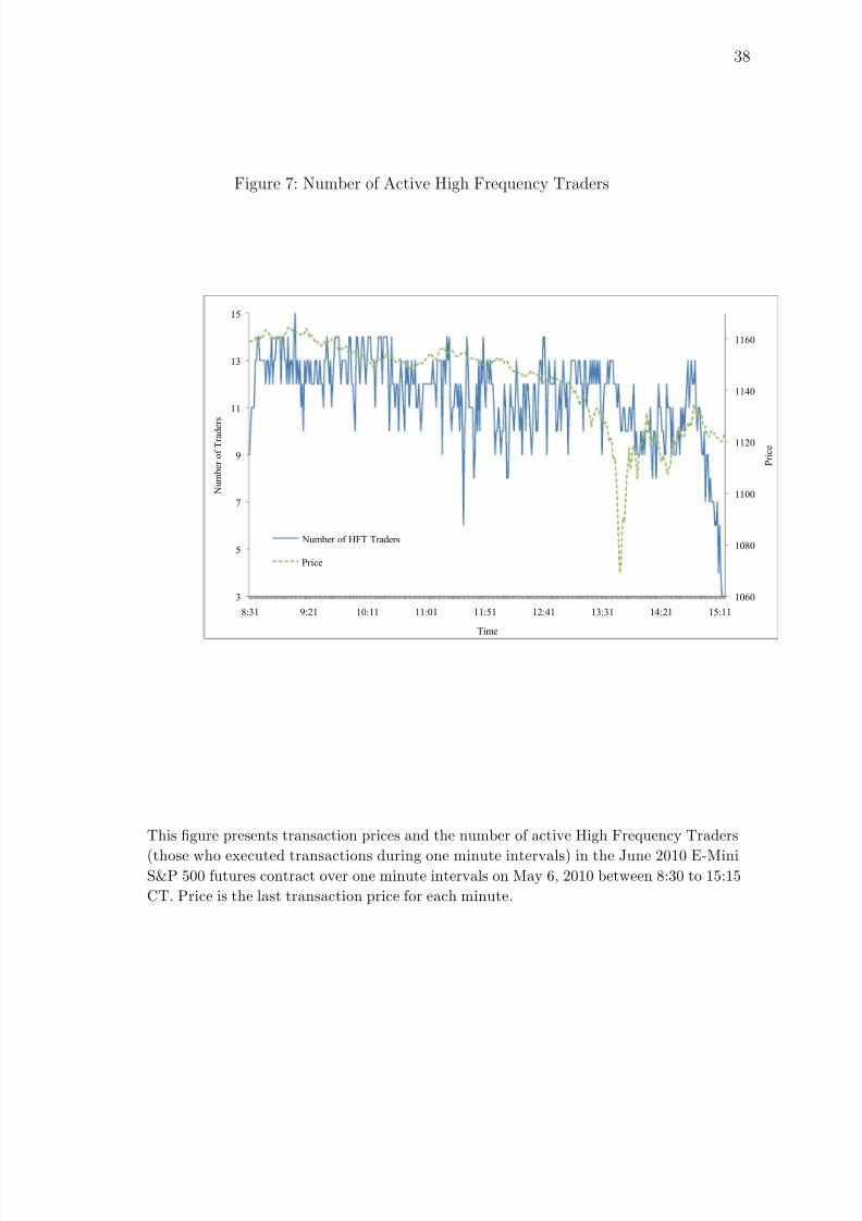
In contrast, as presented in Figure 7, the number of active HFTs decreases from 13 to10.

<Insert Figure 7>



11

Overall, HFTs do not accumulate a significant net position and their position tends toquickly revert to a mean of about zero. Combined with their large share of total tradingvolume (34%), HFTs seem to employ trading strategies to quickly trade through a largenumber of contracts, without ever accumulating a significant net position. These strategiesmay be operating at such a high speed, that they do not seem to be affected by the price

level or price volatility.In contrast to HFTs, Intermediaries tend to revert to their target inventory levels moreslowly. Because of this, on May 6, Intermediaries may have gotten caught on the wrong sideof the market as they bought when prices rapidly fell.

7.2 HFTs and Intermediaries: Net Holdings and Prices

We formally examine the second-by-second trading behavior of HFTs and Intermediaries byexamining empirical regularities between their net holdings and prices. Equation 1 presentsthis in a regression framework.

∆yt = α + ϕ∆yt−1 + δyt−1 +20

i=0

[βt−i ×∆ pt−i/0.25] + ϵt (1)

where yt denotes portfolio holdings of HFTs or Intermediaries during minute t, wheret = 0 corresponds to 8:30 CT. Price changes, ∆ pt−i, i = 0,...,20 are in ticks (0.25 indexpoints) and the change in inventories, ∆yt, is in the number contracts. We interpret δ andϕ as long-term and short-term mean reversion coefficients.10

Table 4 presents estimated coefficients of the regression above. Panels A and B reportthe results for May 3-5 and May 6, respectively. The t statistics are corrected for serialcorrelation, up to twenty seconds, using the Newey-West(1987) estimator.

<Insert Table 4 >

The first column of Panel A presents regression results for HFTs during May 3-5. Thecoefficient estimate for the long-term mean reversion parameter is -0.006, and is statisticallysignificant. This suggests that HFTs reduce 0.6% of their position in one second. Thislong-term mean reversion coefficient corresponds to an estimated half-life of the inventoryholding period of 115 seconds.11 In other words, holding prices constant, HFTs reduce half of their net holdings in 115 seconds.

Changes in net holdings of HFTs are statistically significantly positively related to changes

in prices for the first 5 seconds. The estimated coefficients are positive, consistently decayingfrom the high of 25.416 for the contemporaneous price to the low of 2.248 for the price 5seconds prior. This can be interpreted as follows: a one tick increase in current price corre-sponds to a increase of about 25.4 contracts in the net holdings of HFTs. Moreover, a one

10Dickey-Fuller tests verify that HFT holdings level, Intermediary holdings level, as well as first differencesare stationary. This is consistent with the intraday trading practices of HFTs and Intermediaries to targetinventory levels close to zero.

11We calculate the estimated half-life of the inventory holding period as ln(0.5)(δ) .



12

tick increase in the current price corresponds to an increase of up to 72 contracts during thenext 5 seconds.

In contrast, estimated coefficients for lagged prices 10 to 20 seconds prior to the currentholding period are negative (and statistically significant). These estimated coefficients fallwithin a much more narrow range of -2.257 and -4.585. This, in turn, means that a one tick

increase in price 10 to 20 seconds before corresponds to a maximum cumulative decrease innet holdings of about 34.7 contracts.We interpret these results as follows. HFTs appear to trade in the same direction as the

contemporaneous price and prices of the past five seconds. In other words, they buy, if theimmediate prices are rising. However, after about ten seconds, they appear to reverse thedirection of their trading - they sell, if the prices 10-20 seconds before were rising.

These regression results suggest that, possibly due to their speed advantage or superiorability to predict price changes, HFTs are able to buy right as the prices are about toincrease. HFTs then turn around and begin selling 10 to 20 seconds after a price increase.

The second column of Panel A presents regression results for the Intermediaries on May3-5. Similarly to HFTs, the long term mean reversion coefficient for the Intermediaries is

-0.004 and is statistically significant. This suggests that the Intermediaries reduce their netholdings by 0.4% after one second. The half-life of their inventory is 173 seconds.

In marked contrast to HFTs, coefficient estimates for the contemporaneous price and theprice one second before that are negative (and significant) at -12.045 and -3.046, respectively.However, at prices 3 to 9 seconds prior, the estimated coefficients are positive and significant.

These coefficients could be interpreted as follows. The Intermediaries sell when theimmediate prices are rising, and buy if the prices 3-9 seconds before were rising. Theseregression results suggest that, possibly due to their slower speed or inability to anticipatepossible changes in prices, Intermediaries buy when the prices are already falling and sellwhen the prices are already rising.

Panel B presents the results of equation 1 on May 6th. The first column of Panel B showsthe results for HFTs. The coefficient for the lagged change in holdings parameter is positivebut statistically insignificant at the 5% level. The coefficients for contemporaneous throughthe 3rd lagged price changes are positive, ranging from 4.718 for the contemporaneous pricechange to 0.478 for the 3rd lagged price change.

In contrast to May 3-5, coefficients for the May 6th regressions turn negative (and sig-nificant) by the fourth second. The first negative estimate is for 4th lagged price change,-2.401, suggesting that on May 6, HFTs repeatedly reversed the direction of their trading(e.g., become contrarian, switching from buying to selling, or otherwise) significantly soonerthan during May 3-5.

The second column of Panel B reports the results for the change in holdings of Interme-

diaries on May 6th. The contemporaneous price change estimate is -8.280. The lagged pricechange coefficients become positive for the next 4 lagged price changes, decaying from 3.187to 0.212.

We interpret the difference in results between these two samples to a change in Interme-diary behavior during the Flash Crash. As observed in Section 6, numerous Intermediarieswithdrew during and after the rapid price drop on May 6. Figure 6 shows that the numberof active Intermediaries dropped from 66 to 33 after the large price decline. This may haveto led to a reduction in liquidity provision from this trader category during the Flash Crash.



13

7.3 HFTs and Intermediaries: Liquidity Provision/Removal

We consider Intermediaries and HFTs to be very short term investors. They do not holdpositions over long periods of time and revert to their target inventory level quickly. Observedtrading activity of HFTs can be separated into three parts. First, HFTs seem to anticipateprice changes (in either direction) and trade aggressively to profit from it. Second, HFTs

seem to provide liquidity by putting resting orders in the direction of the anticipated theprice move. Third, HFTs trade to keep their inventories within a target level. The inventory-management trading objective of HFTs may interact with their price-anticipation objective.In other words, at times, inventory-management considerations of HFTs may lead them toaggressively trade in the same direction as the prices are moving, thus, taking liquidity. Atother times, in order to revert to their target inventory levels, HFTs may passively tradeagainst price movements and, thus, provide liquidity.

In order to examine the liquidity providing and taking behavior of HFTs and Inter-mediaries, we separate their changes in holdings into aggressive changes (those incurred viaaggressive acquisitions) and passive changes (those incurred via passive acquisitions). Specif-

ically, when traders submit marketable orders into the order book, they are considered tobe aggressive. Conversely, the traders’ resting orders being executed by a marketable orderresult in passive execution.

Table 5 presents the regression results of the two components of change in holdingson lagged inventory, lagged change in holdings and lagged price changes over one secondintervals. Panel A and Panel B report the results for May 3-5 and May 6th, respectively.

<Insert Table 5 >

The dependent variable in the first column of Panel A is the aggressive change in holdingsof HFTs on May 3-5. The short term and long term mean reversion coefficients are statisti-cally significant, -0.038% and -.005%, respectively. In other words, HFTs aggressively reduce0.5% of their holdings in one second. The coefficient estimates for price changes are positivefor the contemporaneous and first 5 lagged prices, decaying from 48.866 to 3.127. This canbe interpreted as follows: a one tick increase in current price corresponds to an aggressiveincrease of position of about 48.866 contracts by HFTs. Moreover, a one tick increase in thecurrent price corresponds to an increase of up to 102 contracts during the next 5 seconds.

The second column of Panel A presents the regression results for the passive change inholdings of HFTs on May 3-5. The coefficient for lagged change in holdings is 0.034 andstatistically significant. The long term mean reversion estimate is -0.001 which is smaller

than the coefficient from the aggressive holdings change r egression. The coefficient esti-mates for the price changes are almost always negative. The contemporaneous and first 2lagged price changes are negative and statistically significant; ranging from -23.450 for thecontemporaneous price change to -3.766 for the 2nd lagged price change.

Given the difference in magnitude between the aggressive and passive long term meanreversion coefficients, we interpret these results as follows, HFTs may be reducing theirpositions and reacting to anticipated price changes by submitting marketable orders. Inaddition, passive holdings changes of HFTs reflect liquidity provision.



14

The dependent variable in the third column of Panel A is the aggressive holdings changeof the Intermediaries on May 3-5. The coefficients for lagged change in holdings and laggedinventory level are 0.007 and -0.002, respectively. This result corresponds to Intermediariesreducing 0.2% of their holdings aggressively in one second. The coefficients for the currentand lagged price changes are positive; decreasing from 5.264 for the current price change to

0.540 for the 12th lagged price change.These estimates are smaller than the estimates for HFTs. Accordingly, we interpret theseresults as evidence suggesting that Intermediaries are slower than HFTs in responding toanticipated price changes.

The fourth column of Panel A presents the results for the passive position change compo-nent of Intermediaries’ activity. The coefficient estimates for lagged change in holdings andlagged level of holding of Intermediaries are -0.008 and -0.002, respectively. These coefficientsare similar to those we observe from the passive trading of Intermediaries. The coefficientestimates for price changes are statistically negative through the 4th lag. The coefficientsrange from -17.309 for the current price change to -1.157 for the 4th lagged price change.

Our interpretation of these results suggests that given the similar passive and aggressive

mean reversion coefficients, Intermediaries use primarily marketable orders to move to theirtarget inventory level. The passive holdings change for Intermediaries is also contrarian toprice fluctuations, suggesting that the passive holdings change can be a good proxy for theliquidity provision of Intermediaries.

In summary, the larger coefficient for the Aggressive long term mean reversion parameter,suggests that HFTs very quickly reduce their inventories by submitting marketable orders.They also aggressively trade when prices are about to change. Over slightly longer timehorizons, however, HFTs sometimes act as providers of liquidity. In contrast, changes inIntermediary net holdings are negatively correlated with price changes over horizons of up to1 second and positively correlated with price changes over horizons between 3 and 9 seconds.

We interpret this result as evidence that unlike HFTs, Intermediaries provide liquidityover very short horizons and rebalance their portfolios over longer horizons.The first column of Panel B presents the results for aggressive holdings change of HFTs

on May 6th. Only the coefficients on the current and lagged price changes are positive andstatistically significant; 20.341 and 5.457, respectively. The second column of Panel B showsthe results for passive holdings change of HFTs. The contemporaneous price coefficient,-15.622, is statistically significant.

These results are similar to those we observe on the 3 days prior to May 6. Therefore,we interpret these results as evidence that HFTs did not significantly alter their behaviorduring the Flash Crash.

The third column of Panel B presents the results for the aggressive positions change

of Intermediaries. The contemporaneous price change coefficient is 2.894 and statisticallysignificant The fourth column in Panel B displays the results for passive holdings changeof Intermediaries. The contemporaneous price change coefficient is -11.173 and statisticallysignificant.

The coefficients on price changes tend to be larger than those we observe prior to May6th. We interpret this as a possible decrease in liquidity provision by Intermediaries duringthe Flash Crash.



15

7.4 HFTs and Intermediaries: The Flash Crash

To examine these participants’ activity at an even higher resolution during the Flash Crash.We employ equation 1 during the 36-minute period of the Flash Crash - starting at 13:32p.m. and ending at 14:08 p.m. CT. We partition this sample into two subsamples, theprice crash (DOWN, 13:32-13:45 p.m. CT) and recovery (UP, 13:45-14:08 CT), presented in

Panels A and B, respectively of Table 6.

<Insert Table 6 >

The first column of Panel A presents the results for aggressive holdings change of HFTson May 6th during the rapid price decline. The long term mean reversion coefficient is -0.008.The contemporaneous price coefficient is 22.218. Lagged price coeffecients become negativeby the 2nd lag.

The second column of Panel A presents passive change in holding of HFTs during the price

decline. The long term mean reversion coefficient is positive but statistically insignificant.The coeffecient for contemporaneous price is -11.174 and statistically significant.

We interpret these results as follows: HFTs did not alter their behavior significantlywhen prices were rapidly going down. They also appeared to be providing liquidity withtheir passive trading given the coefficients we observe in second column of Panel A.

The third column of Panel A presents the results for Intermediaries’ aggressive positionchange on May 6th during as the price of the E-mini decreased rapidly. The contemporaneousprice coefficient is 3.539 and statistically significant. Price coeffecients remain positive andstatistically significant through the 3rd lag, decaying to 1.794.

The fourth column of Panel A presents results for the passive position changes of HFTs

during the decrease in price. The long term mean reversion coefficient is -0.011 and sta-tistically significant. The coeffecient for contemporaneous price is -10.111 and statisticallysignificant.

These findings are not much different from those we obtain in previous regressions. Ac-cordingly we interpret these results as evidence that intermediaries did not seem to altertheir trading strategies significantly as the price of the E-mini contract declined.

The dependent variable in the first column of Panel B is HFTs aggressive position changewhile the prices are rapidly going up. The long term mean reversion coefficient is -0.005 andis statistically significant. The coefficient for the contemporaneous price change is 0.70 andis statistically insignificant. Coefficients on lagged prices remain insignificant and becomenegative as soon as the first lagged price. These results are quantitatively different than

those we observe in previous regressions.We interpret this lack of statistical significance in the relationship between HFT ag-

gressive net position changes and prices as being related to the influx of opportunistic andfundamental buyers who buoyed the price of the E-mini contract during and after the tradingpause.

The results in the second column of Panel B present the relation between prices and pas-sive net position changes of HFTs when the prices were on their way up. The long term mean



16

reversion coefficient is again insignificant. The statistically significant contemporaneous pricechange coefficient, -10.316, is similar to past regressions of passive holdings changes.

We intrepret these results as a continuation in liquidity provisions by HFTs as the priceof the E-mini contract recovered to levels observed before the Flash Crash.

The third column of Panel B presents the regression results for the aggressive position

change of Intermediaries. The long term mean reversion coefficient is -0.004 and is statis-tically significant. Contemporaneous price change coeffeicent is 1.416 and is statisticallysignificant. This is smaller than the same coefficient during the regression of Intermediaryaggressive holdings changes during the crash.

The fourth column of Panel B lists the regression results where the passive positionchanges of Intermediaries during the price recovery of the E-mini contract. Although thecontemporaneous price coefficient is negative and statistically significant as we observe inprevious regression of Intermediary passive holdings changes, at -3.597, the magnitude of this coefficient is considerably smaller those we observe in the other regressions.

We attribute this decrease in magnitude of contemporaneous price change coefficients toa partial withdrawal we observed by Intermediaries during this time period. However, the

relatively smaller decrease in the aggressive holdings change coefficient compared to that of HFTs may be due to the increased use of market orders Intermediaries used to offset theirdisadvantageous position during the Flash Crash.

7.5 HFTs and Intermediaries: The Hot Potato Effect

A basic characteristic of futures markets is that they remain in zero net supply throughoutthe day. In other words, for each additional contract demanded, there is precisely oneadditional contract supplied. End of day open interest presents a single reading of the levelsof supply and demand at the end of that day.

In intraday trading, changes in net demand/supply result from changes in net holdingsof different traders within a specified period of time, e.g., one minute. These minute byminute changes in the net positions of individual trading accounts can be aggregated to geta minute by minute net change in holdings for our six trader categories. To change their netposition by one contract, a trader may buy one contract or may buy 101 contracts and sell100 contracts.

We examine the ratio of trading volume during one minute intervals to the change in netposition over one minute intervals to study the relationship between High Frequency Tradertrading volume and changes in net position. We calculate the same metric for Intermediariesand find that although High Frequency Traders are active before and during the Flash Crash,they do not significantly change their net positions.

We find that compared to the three days prior to May 6, there was an unusually levelof HFT “hot potato” trading volume — due to repeated buying and selling of contractsaccompanied a relatively small change in net position. The hot potato effect was especiallypronounced between 13:45:13 and 13:45:27 CT, when HFTs traded over 27,000 contracts,which accounted for approximately 49% of the total trading volume, while their net positionchanged by only about 200 contracts.

We interpret this finding as follows: the lack of Opportunistic and Fundamental Trader,as well as Intermediaries, with whom HFTs typically trade, resulted in higher trading vol-



17

ume among HFTs, creating a hot potato effect. It is possible that during the period of high volatility, Opportunistic and Fundamental Traders were either unable or unwilling toefficiently submit orders. In the absence of their usual trading counterparties, HFTs wereleft to trade with other HFTs.

8 Fundamental Traders

Trading volume of the Fundamental Buyers and Sellers accounts for about 10-12% of thetotal trading volume both during May 3-5 and on May 6. However, Fundamental traderstypically remove more liquidity from the market than they provide. As a result, a sizableprogram executed by the Fundamental traders is more likely to have a significant impact onthe market.

In this section we examine the trading behavior of Fundamental traders. We ask thefollowing question: Was the trading behavior of Fundamental Buyers and Sellers differenton May 6, especially during the period of extreme price volatility?

Table 7 presents the average number of contracts bought and sold by different categoriesof traders during two time periods on May 3-5 and on May 6. For both May 3-5 and May 6,the period between 1:32 p.m. and 1:45 p.m. CT is defined as ‘UP’ and the period between1:45 p.m. and 2:08 p.m. CT is defined as ‘DOWN’.

<Insert Table 7 >

According to Table 7, there a significant increase in the number of contracts sold by theFundamental Sellers during the period of extreme price volatility on May 6 compared to thesame period during the previous three days.

Specifically, between 1:32 p.m. and 1:45 p.m. CT, the 13-minute period when the

prices rapidly declined, Fundamental Sellers sold more than 80,000 contracts net, whileFundamental Buyers bought approximately 50,000 contracts net. This level of net sellingby the Fundamental Sellers is about 15 times larger compared to their net selling over thesame 13-minute interval on the previous three days, while the level of net buying by theFundamental Buyers is about 10 times larger compared to their net buying over the sametime period on the previous three days.

In contrast, between 1:45 p.m. and 2:08 p.m. CT, the 23-minute period of the rapidprice rebound, Fundamental Sellers sold more than 110,000 contracts net and FundamentalBuyers bought more than 110,000 contracts net. This level of selling by the FundamentalSellers is about 10 times larger compared than their selling over the same 23-minute interval

on the previous three days, while this level of buying by the Fundamental Buyers is morethan 12 times larger compared to their buying over the same time period on the previousthree days.

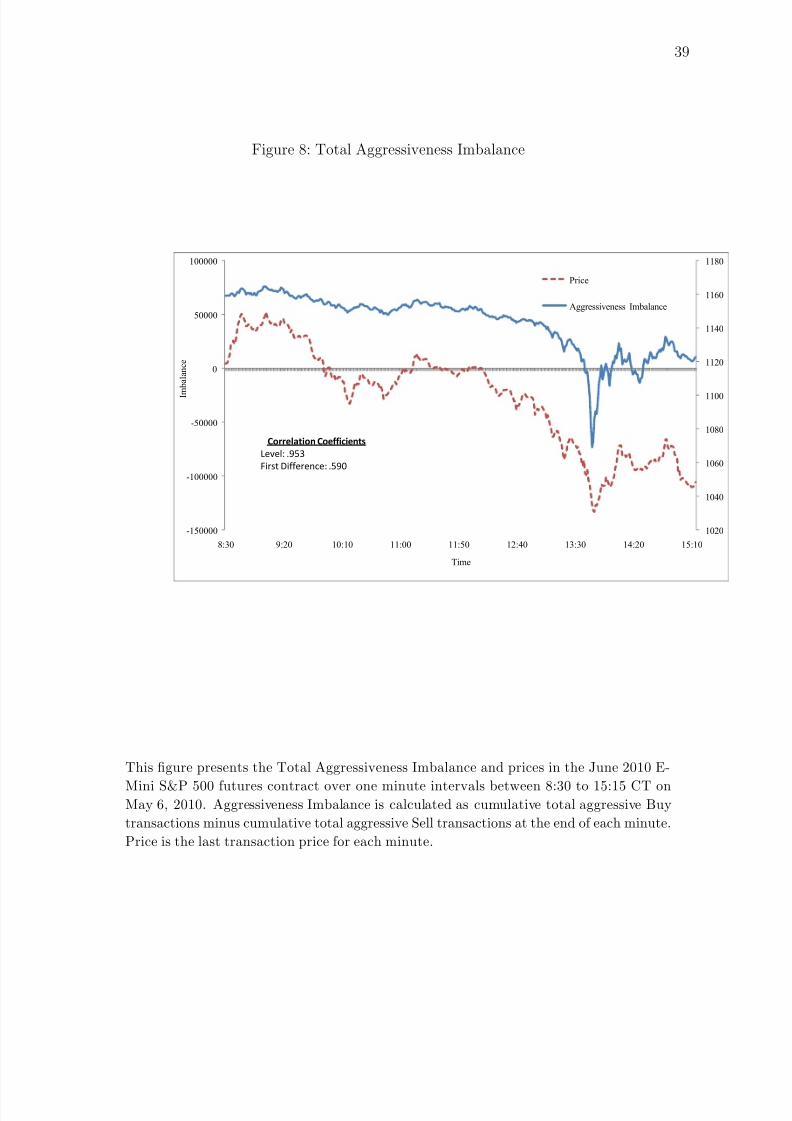
9 Market Impact

We utilize the Aggressiveness Imbalance indicator to estimate the price impacts of varioustrader categories. Aggressiveness Imbalance is an indicator designed to capture the direction



18

of the removal of liquidity from the market. Aggressiveness Imbalance is constructed as thedifference between aggressive buy transactions minus aggressive sell transactions.

Figure 8 shows the relationship between price and cumulative Aggressiveness Imbalance(aggressive buys - aggressive sells).

<Insert Figure 8>

In addition, we calculate Aggressiveness Imbalance for each category of traders over oneminute intervals. For illustrative purposes, the Aggressiveness Imbalance indicator for HFTsand Intermediaries are presented in Figures 9 and 10, respectively.

<Insert Figure 9>

<Insert Figure 10>

According, to Figures 9 and 10, visually, HFTs behave very differently during the FlashCrash compared to the Intermediaries. HFTs aggressively sold on the way down and ag-gressively bought on the way up. IN contrast, Intermediaries are about equally passive andaggressive both down and up.

More formally, we estimate market impact of different categories of traders. The estimatesare obtained by running the following minute-by-minute regressions:

∆P tP t−1 × σt−1

= α +5

i=1

[λi ×AGGi,t

Shri,t−1 × 100, 000] + ϵt (2)

The dependent variable in the regression is the price return scaled by the previous period’svolatility.12 The independent variables in the regression are the aggressiveness imbalance foreach trader category scaled by the category’s lagged share of market volume times 100,000.The Newey-West(1987) estimator t corrects for serial correlation for up to three lags.

Estimated coefficients are presented in Table 8.

<Insert Table 8 >12For the estimate of volatility, we use range - the natural logarithm of the maximum price over the

minimum price.



19

Panel A of Table 8 presents regression results for the period May 3-5. The specificationfits quite well with an R2 of 36% and all estimated price impact coefficients are statisticallysignificant at 5% level.

HFTs and Opportunistic traders have the highest estimated price impact with the coef-ficients of 5.37 and 7.6, respectively. The estimated price impact of the Intermediaries is the

lowest at 0.83. The estimated price impact of the Fundamental Sellers (1.36) is about equalto that of the Fundamental Buyers (1.31).Panel B of Table 8 presents regression results for May 6. The model seems to have a

better fit with an R2 of 59%. All slope coefficients are again statistically significant at 5%level. The estimated price impact of HFTs is smaller at 3.23. In contrast, the estimatesprice impact of the Intermediaries (5.99) is more than seven times larger on May 6 comparedto the previous three days. The estimated price impact of Opportunistic traders on May 6(7.49) is about the same as it is during May 3-5. However, the estimated price impact of Fundamental Sellers (0.53) is nearly double that of the Fundamental Buyers (0.53).

We interpret these results as follows. High Frequency Traders have a large, positivecoefficient possibly due to their ability to anticipate price changes. In contrast, Fundamental

Traders have a much smaller market impact, which is likely due to their explicit tradingstrategies that try to limit market impact, in order to minimize transaction costs.

To illustrate the fit of these regressions, we use the estimated coefficients from the priceimpact regression during May 3-5 to fit minute-by-minute price changes on May 6 (Figure 11).

<Insert Figure 11>

According to Figure 11, the fitted price (marked line) is quite close to the actual price(solid line).

10 Discussion: The Flash Crash

We believe that the events on May 6 unfolded as follows. Financial markets, already tenseover concerns about the European sovereign debt crisis, opened to news concerning theGreek government’s ability to service its sovereign debt. As a result, premiums rose forbuying protection against default on sovereign debt securities of Greece and a number of other European countries. In addition, the S&P 500 volatility index (“VIX”) increased,and yields of ten-year Treasuries fell as investors engaged in a “flight to quality.” By mid-afternoon, the Dow Jones Industrial Average was down about 2.5%.

Sometime after 2:30 p.m., Fundamental Sellers began executing a large sell program.Typically, such a large sell program would not be executed at once, but rather spread outover time, perhaps over hours. The magnitude of the Fundamental Sellers’ trading programbegan to significantly outweigh the ability of Fundamental Buyers to absorb the sellingpressure.

HFTs and Intermediaries were the likely buyers of the initial batch of sell orders fromFundamental Sellers, thus accumulating temporary long positions. Thus, during the early



20

moments of this sell program’s execution, HFTs and Intermediaries provided liquidity to thissell order.

However, just like market intermediaries in the days of floor trading, HFTs and Interme-diaries had no desire to hold their positions over a long time horizon. A few minutes afterthey bought the first batch of contracts sold by Fundamental Sellers, HFTs aggressively sold

contracts to reduce their inventories. As they sold contracts, HFTs were no longer providersof liquidity to the selling program. In fact, HFTs competed for liquidity with the sellingprogram, further amplifying the price impact of this program.

Furthermore, total trading volume and trading volume of HFTs increased significantlyminutes before and during the Flash Crash. Finally, as the price of the E-mini rapidly felland many traders were unwilling or unable to submit orders, HFTs repeatedly bought andsold from one another, generating a “hot-potato” effect.

Yet, Opportunistic Buyers, who may have realized significant profits from this largedecrease in price, did not seem to be willing or able to provide ample buy-side liquidity. Asa result, between 2:45:13 and 2:45:27, prices of the E-mini fell about 1.7%.

At 2:45:28, a 5 second trading pause was automatically activated in the E-mini. Oppor-

tunistic and Fundamental Buyers aggressively executed trades which led to a rapid recoveryin prices. HFTs continued their strategy of rapidly buying and selling contracts, while abouthalf of the Intermediaries closed their positions and got out of the market.

In light of these events, a few fundamental questions arise. Why did it take so longfor opportunistic buyers to enter the market and why did the price concessions had to beso large? It seems possible that some opportunistic buyers could not distinguish betweenmacroeconomic fundamentals and market-specific liquidity events. It also seems possible thatthe opportunistic buyers have already accumulated a significant positive inventory earlier inthe day as prices were steadily declining. Furthermore, it is possible that they could notquickly find opportunities to hedge additional positive inventory in other markets which also

experienced significant volatility and higher latencies. An examination of these hypothesesrequires data from all venues, products, and traders on the day of the Flash Crash.

11 Conclusion

In this paper, we analyze the behavior of High Frequency Traders and other categories of traders during the extremely volatile environment on May 6, 2010.

Based on our analysis, we believe that High Frequency Traders exhibit trading patternsconsistent with market making. In doing so, they provide very short term liquidity totraders who demand it. This activity comprises a large percentage of total trading volume,

but does not result in a significant accumulation of inventory. As a result, whether undernormal market conditions or during periods of high volatility, High Frequency Traders arenot willing to accumulate large positions or absorb large losses. Moreover, their contributionto higher trading volumes may be mistaken for liquidity by Fundamental Traders. Finally,when rebalancing their positions, High Frequency Traders may compete for liquidity andamplify price volatility.

Consequently, we believe, that irrespective of technology, markets can become fragilewhen imbalances arise as a result of large traders seeking to buy or sell quantities larger



21

than intermediaries are willing to temporarily hold, and simultaneously long-term suppliersof liquidity are not forthcoming even if significant price concessions are offered.

We believe that technological innovation is critical for market development. However,as markets change, appropriate safeguards must be implemented to keep pace with tradingpractices enabled by advances in technology.

References

Alfonsi, A., A. Fruth, and A. Schied, 2008, “Constrained Portfolio Liquidation in a LimitOrder Book Model,” Banach Center Publ. 83, 9–25.

Almgren, R. and N. Chriss, 1999, “Value Under Liquidation,” Risk 12, 61-63.

Almgren, R. and N. Chriss, 2000, “Execution of Portfolio Transactions,” J. Risk 3, 5-39.

Almgren, R. and J. Lorenz, 2006, “Bayesian Adaptive Trading With a Daily Cycle,” J.

Trading 1, 38-46.

Amihud, Y., H. Mendelson, and L. Pedersen, 2005, “Liquidity and Asset Prices,” NOW-

publishers.com .

Berkman, H., 1996, “Large Option Trades, Intermediaries and Limit Orders,” Review of

Financial Studies 9, 977–1002.

Bertsimas, D. and A. Lo 1998, “Optimal Control of Execution Costs,” Journal of Financial

Markets 1, 1–50.

Biais, B., L. Glosten, and C. Spatt, 2002, “Market Microstructure: A Survey of Microfoun-

dations, Empirical Results, and Policy Implications,” Journal of Financial Markets 8,217–264.

Biais, B., D. Martimort, and J. Rochet, 2000, “Competing Mechanisms in a Common ValueEnvironment,” Econometrica 68, 799–838.

Black, B., 1971, “Towards a Fully Automated Exchange, Part I,” Financial Analysts Jour-

nal 27, 29-34.

Brunnermeier, M. and L. Pedersen, 2005, “Predatory Trading,” Journal of Finance 60,1825-1863.

Carlin, B., M. Lobo, and S. Viswanathan, 2007, ”Episodic Liquidity Crises: Cooperativeand Predatory Trading,” Journal of Finance 62, 2235–2274.

Cespa, G. and T. Foucault, 2008, “Insiders-Outsiders, Transparency, and the Value of theTicker,”Working Paper .

Chan, L. and J. Lakonishok, 1993, “The Behavior of Stock Prices Around InstitutionalTrades,” Journal of Financial Economics 33, 173–200.



22

Chan, L. and J. Lakonishok, 1995, “Institutional Trades and Intra-Day Stock Price Behav-ior,” Journal of Finance 50, 1147–1174.

Chiyachantana, C., P. Jain, C. Jiang, and R. Wood, 2004, “International Evidence onInstitutional Trading Behavior and Determinants of Price Impact,” Journal of Finance

59, 865–894.

Cvitanic, J., and A. Kirilenko, 2010, “High Frequency Traders and Asset Prices,” Working

Paper .

Engle, R. and R. Ferstenberg, 2007, “Execution Risk,” Journal of Portfolio Management ,33, 34–45.

Foucault, T., 1999, “Order Flow Composition and Trading Costs in a Dynamic Limit OrderMarket,” Journal of Financial Markets, 2, 99–134.

Glosten, L. and P. Milgrom, 1985, “Bid, Ask and Transaction Prices in a Specialist Market

with Heterogeneously Informed Traders”Journal of Financial Economics

14, 71–100.Glosten, L. and P. Milgrom, 1989, “Insider Trading, Liquidity, and the Role of the Monop-

olist Specialist” Journal of Business 62, 211–236.

Goettler, R., C. Parlour, and U. Rajan, 2005, “Equilibrium in a Dynamic Limit OrderMarket,” Journal of Finance 60, 2149–2192.

Goettler, R., C. Parlour, and U. Rajan, 2009, “Informed Traders and Limit Order Markets,”Journal of Financial Economics 93, 67–87.

Hasbrouck, J., 2003, “Intraday Price Formation in U.S. Equity Index Markets,” Journal of

Finance 58, 2375–2400.Hasbrouck, J. and G. Saar, 2009, “Technology and Liquidity Provision: The Blurring of

Traditional Definitions,” Journal of Financial Markets 12, 143–172.

Hendershott, T., C. Jones, and A. Menkveld, 2010, “Does Algorithmic Trading ImproveLiquidity?” Journal of Finance Forthcoming.

Hendershott, T. and R. Riordan, 2009, “Algorithmic Trading and Information” Working

Paper .

Holthausen, R., R Leftwich, and D. Mayers, 1987, “The Effect of Large Block Transactions

on Security Prices: A Cross-Sectional Analysis,” Journal of Financial Economics 19,43–172.

Holthausen, R., R. Leftwich, and D. Mayers, 1990, “Large-Block Transactions, the Speed of Response, and Temporary and Permanent Stock Price Effects,” Journal of Financial

Economics 26, 71–95.

Keim, D. and A. Madhavan, 1996, “The Upstairs Market for Large-Block Transactions:Analysis and Measurement of Price Effects,” Review of Financial Studies 9, 1–36.



23

Keim, D. and A. Madhavan, 1997, “Transactions Costs and Investment Style: An Inter-Exchange Analysis of Institutional Equity Trades,” Journal of Financial Economics

46, 265–292.

Kraus, A. and H. Stoll, 1972, “Price Impacts of Block Trading on the New York StockExchange,” Journal of Finance 27, 569–588.

Kyle, A., 1985, “Continuous Auctions and Insider Trading,” Econometrica , 53, 1315–1335.

Madhavan A., 2000, “Market Microstructure: a Survey,” Journal of Financial Markets 3,205–258.

Moallemi C., B. Park, and B. Van Roy, 2009, “Strategic Execution in the Presence of anUninformed Arbitrageur,” Working Paper .

Moallemi C. and M. Saglam, 2010, “The Cost of Latency,” Working Paper .

Newey, W. and K. West, 1987, “A Simple, Positive Semi-Definite, Heteroskedasticity andAutocorrelation Consistent Covariance Matrix,” Econometrica , 55, 703–765.

Obizhaeva A. and J. Wang, 2006, “Optimal Trading Policy and Demand/ Supply Dynam-ics,” Working Paper .

Parlour, C., 1998, “Price Dynamics in Limit Order Markets” Review of Financial Studies

11, 789–816.

Rosu, I., 2009, “A Dynamic Model of the Limit Order Book,” Review of Financial Studies

22, 4601–4641.

Schied, A. and T. Schnenborn, 2007, “Optimal Portfolio Liquidation for CARA Investors,”Working Paper .



24

Table 1: Market Descriptive Statistics

May 3-5 May 6thVolume 2,397,639 5,094,703

# of Trades 446,340 1,030,204# of Traders 11,875 15,422Trade Size 5.41 4.99Order Size 10.83 9.76

Limit Orders % Volume 95.45% 92.44%Limit Orders % Trades 94.36% 91.75%

Volatility 1.54% 9.82%Return -0.02% -3.05%

This table presents summary statistics for the June 2010 E-Mini

S&P 500 futures contract. The first column presents averagescalculated for May 3-5, 2010 between 8:30 and 15:15 CT. The

second column presents statistics for May 6t, 2010 between 8:30

to 15:15 CT. Volume is the number of contracts traded. The num-

ber of traders is the number of trading accounts that traded at

least once during a trading day. Order size and trade sizes are

measured in the number of contracts. Use of limit orders are pre-

sented both in percetn of the number of transactions and trading

volume. Volatility is calculated as range, the natural logarithm of

maximum price over minimum price within a trading day.



25

T a b l e 2 : S u m

m a r y S t a t i s t i c s o f T r a d e r C a t e g o r i e s

P a n e l A : M a y 3 - 5

T r a d e r T y p e

% V o l u m e

% o f T r a d e s

# T r a d e r s

T r a d e S i z e

O r d e r S i z e

L i m i t O r d e r s


A g g R a t i o

A g g R a t i o

( A v g . )

( A v g . )

% V o l u m e

% T r a d e s

T r a d

e - W e i g h t e d

V o l - W e i g h t e d

H i g h F r e q u e n c y T r a d e r

3 4 . 2 2 %

3 2 . 5 6 %

1 5

5 . 6 9

1 4 . 7 5

1 0 0 . 0 0 0 %

1 0 0 . 0 0 0 %

4 9 . 9 1 %

4 5 . 6 8 %

I n t e r m e d i a r y

1 0 . 4 9 %

1 1 . 6 3 %

1 8 9

4 . 8 8

7 . 9 2

9 9 . 6 1 4 %

9 8 . 9 3 9 %

4 3 . 1 0 %

4 1 . 6 2 %

B u y e r

1 1 . 8 9 %

1 0 . 1 5 %

1 , 0 1 3

6 . 3 4

1 4 . 0 9

9 1 . 2 5 8 %

9 1 . 2 7 3 %

6 6 . 0 4 %

6 4 . 0 9 %

S e l l e r

1 2 . 1 1 %

1 0 . 1 0 %

1 , 0 8 8

6 . 5 0

1 4 . 2 0

9 2 . 1 7 6 %

9 1 . 3 6 0 %

6 2 . 8 7 %

6 1 . 1 3 %

O p p o r t u n i s t i c T r a d e r

3 0 . 7 9 %

3 3 . 3 4 %

3 , 5 0 4

4 . 9 8

8 . 8 0

9 2 . 1 3 7 %

9 0 . 5 4 9 %

5 5 . 9 8 %

5 4 . 7 1 %

N o i s e T r a d e r

0 . 5 0 %

2 . 2 2 %

6 , 0 6 5

1 . 2 2

1 . 2 5

7 0 . 0 9 2 %

7 1 . 2 0 5 %

5 9 . 0 4 %

5 9 . 0 6 %

V o l u m e

# o f T r a d e s

# T r

a d e r s

T r a d e S i z e

O r d e r S i z e



V o l a t i l i t y

R e t u r n

( A v g . )

( A v g . )

% V o l u m e

% T r a d e s

A l l

2 , 3 9 7 , 6 3 9

4 4 6 , 3 4 0

1

1 , 8 7 5

5 . 4 1

1 0 . 8 3

9 5 . 4 5 %

9 4 . 3 6 %

1 . 5 4 %

- 0 . 0 2 %

P a n e l B : M a y 6 t h

T r a d e r T y p e

% V o l u m e

% o f T r a d e s

# T r a d e r s

T r a d e S i z e

O r d e r S i z e



A g g R a t i o

A g g R a t i o

( A v g . )

( A v g . )

% V o l u m e

% T r a d e s

T r a d

e - W e i g h t e d

V o l - W e i g h t e d

H i g h F r e q u e n c y T r a d e r

2 8 . 5 7 %

2 9 . 3 5 %

1 6

4 . 8 5

9 . 8 6

9 9 . 9 9 7 %

9 9 . 9 9 7 %

5 0 . 3 8 %

4 5 . 5 3 %

I n t e r m e d i a r y

9 . 0 0 %

1 1 . 4 8 %

1 7 9

3 . 8 9

5 . 8 8

9 9 . 6 3 9 %

9 9 . 2 3 7 %

4 5 . 1 8 %

4 3 . 5 5 %

B u y e r

1 2 . 0 1 %

1 1 . 5 4 %

1 , 2 6 3

5 . 1 5

1 0 . 4 3

8 8 . 8 4 1 %

8 9 . 5 8 9 %

6 4 . 3 9 %

6 1 . 0 8 %

S e l l e r

1 0 . 0 4 %

6 . 9 5 %

1 , 2 7 6

7 . 1 9

2 1 . 2 9

8 9 . 9 8 5 %

8 8 . 9 6 6 %

6 8 . 4 2 %

6 5 . 6 8 %

O p p o r t u n i s t i c T r a d e r

4 0 . 1 3 %

3 9 . 6 4 %

5 , 8 0 8

5 . 0 5

1 0 . 0 6

8 7 . 3 8 5 %

8 5 . 3 5 2 %

6 1 . 9 2 %

6 0 . 2 8 %

N o i s e T r a d e r

0 . 2 5 %

1 . 0 4 %

6 , 8 8 0

1 . 2 0

1 . 2 4

6 3 . 6 0 9 %

6 4 . 8 7 9 %

6 3 . 4 9 %

6 3 . 5 3 %

V o l u m e

# o f T r a d e s

# T r

a d e r s

T r a d e S i z e

O r d e r S i z e



V o l a t i l i t y

R e t u r n

( A v g . )

( A v g . )

% V o l u m e

% T r a d e s

A l l

5 , 0 9 4 , 7 0 3

1 , 0 3 0 , 2 0 4

1

5 , 4 2 2

4 . 9 9

9 . 7 6

9 2 . 4 4 3 %

9 1 . 7 5 0 %

9 . 8 2 %

- 3 . 0 5 %

T h i s t a b l e p r e s e n t s s u m m a r y s t a t i s t i c s f o r t r a d e r c a t e g o r i e s a n d t h e o v e r a l l m a r k

e t . T h e fi r s t c o l u m n p r e s e n t s s t

a t i s t i c s p r i o r t o M a y 6 a s t h e

a v e r a g e o v e r t h r e e t r a d i n g d a y s , M a y 3 - 5 , 2 0 1 0 f r o m 8 : 3 0 t o 1 5 : 1 5 C T . T h e s e c o n

d c o l u m n p r e s e n t s s t a t i s t i c s f o r M a y 6 f r o m 8 : 3 0 t o 1 5 : 1 5 C T .



26

T

a b l e 3 : O r d e r P r o p e r t i e s

P a n e l A : M a y 3 - 5

O r d e r A g g r e s s i v e n e s s D i s t r i b u t i o n

A v g O r d e r S i z e

A v g # o

f T r a d e s P e r O r d e r

H F T

M

M

B u y e r

S e l l e r

O p p o r .

N o

i s e

H F T

M M

B u y e r

S e l l e r

O p p o r .

N o i s e

H F T

M M

B u y e r

S e l l e r

O p p o r .

N o i s e

A g g = 0

7 8 . 7

6 %

7 8 . 6 1 %

5 3 . 0

2 %

5 2 . 2

2 %

6 0 . 4

3 %

4 3 . 1 1 %

7 . 3

9

6 . 3

1

1 0 . 2

5

1 0 . 3 2

6 . 3

7

1 . 2

0

1 . 4

4

1 . 3

7

1 . 5

1

1 . 4

6

1 . 3

4

1 . 0

1

A g g < = 0 . 1

7 8 . 9

4 %

7 8 . 6 6 %

5 3 . 0

6 %

5 2 . 2

5 %

6 0 . 4

7 %

4 3 . 1 1 %

8 8 . 2

2

5 2 . 6

4

2 1 8 . 0

7

1 0 6 . 9 7

2 3 9 . 0

6

0 . 0

0

1 1 . 6

1

8 . 2

9

4 7 . 7

1

1 0 . 5

8

4 0 . 9

8

0 . 0

0

A g g < = 0 . 2

7 9 . 1

5 %

7 8 . 7 2 %

5 3 . 1

1 %

5 2 . 2

8 %

6 0 . 5

1 %

4 3 . 1 1 %

1 0 8 . 3

8

5 0 . 8

5

8 3 . 6

4

1 0 8 9 . 0 6

3 1 9 . 8

1

0 . 0

0

1 4 . 1

0

9 . 6

7

9 . 0

6

1 9 5 . 1

8

4 9 . 9

0

0 . 0

0

A g g < = 0 . 3

7 9 . 3

4 %

7 8 . 8 0 %

5 3 . 1

7 %

5 2 . 3

2 %

6 0 . 5

5 %

4 3 . 1 1 %

1 3 3 . 6

7

4 4 . 8

7

3 2 9 . 5

5

3 5 3 . 9 3

3 0 4 . 8

7

4 . 0

0

1 8 . 7

7

9 . 2

6

5 3 . 8

3

3 5 . 6

1

4 6 . 1

9

4 . 0

0

A g g < = 0 . 4

7 9 . 6

1 %

7 8 . 9 1 %

5 3 . 2

3 %

5 2 . 3

6 %

6 0 . 6

0 %

4 3 . 1 1 %

1 0 3 . 1

6

2 4 . 1

6

1 5 0 . 0

1

4 7 4 . 3 8

2 7 5 . 3

8

0 . 0

0

1 6 . 2

9

6 . 3

1

1 9 . 4

8

6 1 . 7

0

4 5 . 7

8

0 . 0

0

A g g < = 0 . 5

8 0 . 0

6 %

7 9 . 1 7 %

5 3 . 3

8 %

5 2 . 4

6 %

6 0 . 6

9 %

4 3 . 1 1 %

9 4 . 9

0

1 4 . 9

3

1 1 5 . 8

0

1 1 2 . 6 2

1 2 1 . 3

4

2 . 0

0

1 4 . 8

2

4 . 4

0

1 5 . 8

4

1 4 . 8

5

1 8 . 2

6

2 . 0

0

A g g < = 0 . 6

8 0 . 2

5 %

7 9 . 2 3 %

5 3 . 4

3 %

5 2 . 5

0 %

6 0 . 7

4 %

4 3 . 1 1 %

2 1 9 . 6

0

5 0 . 0

6

2 7 3 . 7

6

3 4 4 . 4 9

2 3 8 . 2

7

0 . 0

0

3 5 . 7

8

1 1 . 0

7

4 5 . 8

1

5 4 . 1

9

3 7 . 5

4

0 . 0

0

A g g < = 0 . 7

8 0 . 4

8 %

7 9 . 3 3 %

5 3 . 5

2 %

5 2 . 5

6 %

6 0 . 7

9 %

4 3 . 1 1 %

1 9 6 . 9

0

3 9 . 4

2

2 3 5 . 2

4

3 1 4 . 9 4

2 1 1 . 1

0

0 . 0

0

3 2 . 4

0

9 . 9

7

3 9 . 7

0

5 0 . 2

1

3 4 . 1

1

0 . 0

0

A g g < = 0 . 8

8 0 . 6

9 %

7 9 . 4 1 %

5 3 . 5

8 %

5 2 . 6

3 %

6 0 . 8

3 %

4 3 . 1 1 %

2 5 2 . 4

2

5 8 . 4

4

2 5 9 . 4

7

2 4 2 . 9 0

2 1 4 . 2

9

0 . 0

0

4 3 . 7

5

1 4 . 2

9

3 8 . 6

8

3 7 . 5

2

3 5 . 4

3

0 . 0

0

A g g < = 0 . 9

8 0 . 9

2 %

7 9 . 4 8 %

5 3 . 6

7 %

5 2 . 7

0 %

6 0 . 8

8 %

4 3 . 1 1 %

2 4 1 . 2

4

5 4 . 5

5

2 6 7 . 8

8

3 1 1 . 0 9

2 4 8 . 3

2

0 . 0

0

4 2 . 9

5

1 3 . 7

2

4 4 . 3

6

4 9 . 2

2

4 4 . 2

8

0 . 0

0

A g g < 1

8 1 . 3

1 %

7 9 . 5 7 %

5 3 . 7

3 %

5 2 . 7

7 %

6 0 . 9

2 %

4 3 . 1 1 %

2 3 0 . 6

9

7 6 . 0

2

2 0 0 . 3

2

2 9 3 . 6 9

3 4 3 . 0

5

0 . 0

0

4 2 . 1

8

1 6 . 1

0

3 7 . 1

6

4 4 . 9

9

5 5 . 8

0

0 . 0

0

A g g < = 1

1 0 0 . 0

0 %

1 0 0 . 0 0 %

1 0 0 . 0

0 %

1 0 0 . 0

0 %

1 0 0 . 0

0 %

1 0 0 . 0 0 %

2 5 . 2

9

1 2 . 6

2

1 5 . 5

7

1 5 . 0 2

9 . 6

4

1 . 2

8

4 . 2

6

2 . 3

0

2 . 5

3

2 . 4

5

1 . 9

9

1 . 0

3

P a n e l B : M a y 6

O r d e r A g g r e s s i v e n e s s D i s t r i b u t i o n

A v g O r d e r S i z e

A v g # o

f T r a d e s P e r O r d e r

H F T

M

M

B u y e r

S e l l e r

O p p o r .

N o

i s e

H F T

M M

B u y e r

S e l l e r

O p p o r .

N o i s e

H F T

M M

B u y e r

S e l l e r

O p p o r .

N o i s e

A g g = 0

7 8 . 9

2 %

7 5 . 4 7 %

4 4 . 6

7 %

5 9 . 0

1 %

5 3 . 9

5 %

3 8 . 4 8 %

5 . 4

9

5 . 0

7

7 . 7

2

1 2 . 7 4

7 . 3

5

1 . 1

7

1 . 3

5

1 . 3

4

1 . 3

8

1 . 5

8

1 . 4

4

1 . 0

1

A g g < = 0 . 1

7 9 . 2

7 %

7 5 . 5 8 %

4 4 . 7

4 %

5 9 . 1

3 %

5 4 . 0

3 %

3 8 . 4 8 %

6 0 . 2

1

3 0 . 5

8

1 6 0 . 0

2

3 6 9 . 4 4

2 0 8 . 9

8

0 . 0

0

8 . 6

0

5 . 7

9

1 2 . 0

5

3 1 . 0

0

2 8 . 1

0

0 . 0

0

A g g < = 0 . 2

7 9 . 6

0 %

7 5 . 7 2 %

4 4 . 8

7 %

5 9 . 2

7 %

5 4 . 1

5 %

3 8 . 4 8 %

4 9 . 1

3

1 8 . 7

1

2 3 8 . 7

1

2 9 0 . 5 5

1 9 1 . 9

0

0 . 0

0

8 . 3

7

4 . 6

1

3 2 . 8

9

3 1 . 0

8

3 5 . 6

7

0 . 0

0

A g g < = 0 . 3

7 9 . 8

5 %

7 5 . 8 5 %

4 4 . 9

8 %

5 9 . 4

3 %

5 4 . 2

3 %

3 8 . 4 8 %

5 5 . 2

2

1 2 . 7

7

3 9 0 . 7

9

3 1 4 . 1 3

1 5 0 . 9

9

0 . 0

0

9 . 7

6

4 . 1

4

7 6 . 6

9

3 1 . 1

4

2 3 . 3

0

0 . 0

0

A g g < = 0 . 4

8 0 . 1

5 %

7 6 . 1 8 %

4 5 . 1

3 %

5 9 . 5

7 %

5 4 . 3

4 %

3 8 . 4 8 %

5 6 . 7

0

1 2 . 1

9

1 1 0 . 5

4

2 1 8 . 3 6

1 0 5 . 8

7

0 . 0

0

1 0 . 2

0

3 . 9

3

1 4 . 3

6

3 2 . 5

2

1 6 . 0

9

0 . 0

0

A g g < = 0 . 5

8 0 . 5

1 %

7 6 . 8 1 %

4 5 . 7

6 %

5 9 . 8

2 %

5 4 . 4

8 %

3 8 . 4 8 %

5 1 . 5

0

5 . 4

6

2 3 . 8

5

1 7 5 . 7 2

7 8 . 9

0

5 . 0

0

9 . 9

5

2 . 6

5

4 . 6

5

2 7 . 1

3

1 3 . 0

5

2 . 0

0

A g g < = 0 . 6

8 0 . 7

1 %

7 6 . 9 2 %

4 5 . 8

9 %

5 9 . 9

5 %

5 4 . 5

7 %

3 8 . 4 8 %

1 0 6 . 7

2

1 8 . 1

9

1 1 5 . 9

3

2 2 4 . 1 6

1 5 5 . 7

7

0 . 0

0

1 9 . 1

5

5 . 7

5

1 9 . 4

8

3 1 . 7

9

2 5 . 3

7

0 . 0

0

A g g < = 0 . 7

8 0 . 9

6 %

7 7 . 1 0 %

4 6 . 1

1 %

6 0 . 0

7 %

5 4 . 6

5 %

3 8 . 4 8 %

8 3 . 1

1

1 3 . 7

5

7 7 . 6

5

2 9 7 . 3 5

1 6 9 . 4

5

0 . 0

0

1 6 . 4

4

4 . 1

3

1 4 . 4

3

4 5 . 4

9

2 8 . 2

6

0 . 0

0

A g g < = 0 . 8

8 1 . 1

8 %

7 7 . 2 6 %

4 6 . 3

3 %

6 0 . 2

0 %

5 4 . 7

6 %

3 8 . 4 8 %

1 0 1 . 3

6

1 6 . 5

7

9 4 . 0

0

2 5 2 . 7 0

1 3 9 . 1

0

0 . 0

0

1 9 . 0

1

5 . 4

8

1 6 . 2

8

4 3 . 6

7

2 7 . 5

6

0 . 0

0

A g g < = 0 . 9

8 1 . 4

0 %

7 7 . 3 5 %

4 6 . 5

0 %

6 0 . 3

4 %

5 4 . 8

3 %

3 8 . 4 8 %

1 3 2 . 7

2

2 9 . 5

1

8 7 . 6

8

3 0 5 . 8 3

1 7 5 . 5

8

0 . 0

0

2 5 . 2

7

8 . 1

9

1 6 . 0

4

5 0 . 0

3

3 2 . 5

5

0 . 0

0

A g g < 1

8 1 . 7

0 %

7 7 . 4 0 %

4 6 . 6

0 %

6 0 . 4

9 %

5 4 . 9

0 %

3 8 . 4 8 %

1 6 2 . 1

3

4 3 . 5

4

1 8 1 . 9

6

2 8 2 . 3 4

2 1 9 . 1

2

0 . 0

0

3 0 . 8

4

1 0 . 3

5

3 3 . 1

1

4 2 . 1

8

4 0 . 7

4

0 . 0

0

A g g < = 1

1 0 0 . 0

0 %

1 0 0 . 0 0 %

1 0 0 . 0

0 %

1 0 0 . 0

0 %

1 0 0 . 0

0 %

1 0 0 . 0 0 %

1 7 . 7

0

7 . 8

6

9 . 2

8

2 4 . 9 0

1 0 . 2

9

1 . 2

8

3 . 0

7

1 . 8

6

2 . 0

1

3 . 8

4

2 . 1

9

1 . 0

4

T h i s t a b l e r e p o r t s o r d e r s t a t i s t i c s a c r o s s t r a d e r c a t e g o r i e s . T h e o r d e r a g g r e s s i v e n e s s i s d e fi n e d a s t h e r a t i o o f s i z

e o f t h e a g g r e s s i v e p o r t i o n o f

t h e e x e c u t i o n o v

e r o r d e r s i z e . T h e o r d e r a g g r e s s i v e n e s s d i s t r i b u t i o n i s c u m u l a t e d o v e r v a r i o u s a g g r e s s i v e n e s s r a t i o s . A v e r a g e o r d e r s i z e a n d

a v e r a g e n u m b e r o f t r a d e s a r e d i s t r i b u t e d o v e r v a r i o u s o r d e r a g g r e s s i v e n e s s r a t i o s . A v e r a g e o r d e r s i z e i s t h e a v e r a g e n u m b e r o f c o n t r a c t s t r a d e d

p e r o r d e r . A v e r a

g e n u m b e r o f t r a d e s i s t h e a v e r a

g e n u m b e r o f t r a d e s a n o r d e r g e n e r a t e s .



27

Table 4: HFTs and Intermediaries: Net Holdings and Prices

Panel A: May 3-5 Panel B: May 6

∆ NP HFT ∆ NP INT ∆ NP HFT ∆ NP INT

Intercept -1.646 -0.533 Intercept -3.224 0.031(-3.830) (-3.744) (-3.525) (0.120)

∆ NP HF T t−1 -0.004 ∆ NP HF T t−1 0.012(-0.491) (1.339)

NP HF T t−1 -0.006 NP HF T t−1 -0.005(-11.612) (-7.581)

∆ NP IN T t−1 -0.001 ∆ NP INT t−1 -0.019(-0.113) (-1.429)

NP IN T t−1 -0.004 NP INT t−1 -0.008(-10.325) (-8.494)

∆P t 25.416 -12.045 ∆P t 4.718 -8.280(17.377) (-22.684) (2.686) (-8.280)

∆P t−1 19.322 -3.046 ∆P t−1 7.026 2.856(15.413) (-7.553) (6.874) (7.083)

∆P t−2 12.262 0.357 ∆P t−2 1.146 3.187(11.724) (0.966) (1.358) (6.312)

∆P t−3 7.722 1.273 ∆P t−3 0.478 1.979(8.021) (3.589) (0.468) (5.118)

∆P t−4 5.006 2.420 ∆P t−4 -2.401 0.212(5.389) (6.712) (-2.201) (0.670)

∆P t−5 2.248 2.473 ∆P t−5 -1.716 -0.210(2.351) (7.089) (-1.827) (-0.675)

∆P t−6 0.822 1.754 ∆P t−6 0.557 -0.098(0.855) (4.987) (0.621) (-0.292)

∆P t−7 0.141 1.837 ∆P t−7 -3.632 -0.040(0.163) (5.347) (-3.782) (-0.128)

∆P t−8 -1.285 1.329 ∆P t−8 -2.609 -0.893(-1.295) (4.141) (-2.631) (-2.666)

∆P t−9 -1.799 0.864 ∆P t−9 -1.242 -0.320(-1.909) (2.780) (-1.273) (-1.150)

∆P t−10 -2.625 0.447 ∆P t−10 -3.184 -0.743(-2.984) (1.381) (-4.133) (-2.752)

∆P t−11 -2.434 0.136 ∆P t−11 -0.723 -1.091(-2.856) (0.441) (-0.849) (-3.529)

∆P t−12 -3.149 0.059 ∆P t−12 0.149 -0.897(-3.634) (0.198) (0.143) (-3.259)

∆P t−13 -3.062 -0.174 ∆P t−13 2.173 -0.192(-3.553) (-0.528) (1.361) (-0.658)

∆P t−14 -4.585 0.359 ∆P t−14 -1.256 -0.733(-5.183) (1.136) (-1.528) (-2.494)

∆P t−15 -3.796 -0.064 ∆P t−15 0.282 -0.173(-4.353) (-0.204) (0.258) (-0.634)

∆P t−16 -3.842 -0.472 ∆P t−16 -0.827 -0.114(-4.439) (-1.490) (-0.839) (-0.386)

∆P t−17 -2.257 -0.043 ∆P t−17 -0.673 -0.224(-2.652) (-0.132) (-0.703) (-0.668)

∆P t−18 -3.318 -0.152 ∆P t−18 -0.680 -0.266(-3.679) (-0.486) (-0.637) (-0.931)

∆P t−19 -2.773 0.600 ∆P t−19 -0.964 -0.465(-3.164) (1.854) (-1.359) (-1.339)

∆P t−20 -3.108 -0.121 ∆P t−20 -1.560 0.026(-3.931) (-0.431) (-1.448) (0.080)

# obs 72837 72837 #obs 24275 24275Adj −R2 0.0211 0.0337 Adj −R2 0.0099 0.0599

This table displays estimated coefficients of the following regression: ∆yt = α + ϕ∆yt−1 + δyt−1 +∑20i=0[βt−i×∆ pt−i/0.25]+ ϵt. The dependent variable is changes in holdings of High Frequency Traders

and Intermediaries, respectively. Both changes in holdings, ∆yt, and lagged holdings, yt, are in the

number of contracts. Price changes, ∆ pt, are in ticks. Estimates are computed for second-by-second

observations. The t statistics are corrected for serial correlation, up to twenty seconds, using the Newey-

West (1987) estimator. t values reported in parentheses are in bold if the coefficients are statistically

significant at the 5% level.



28

Table 5: HFTs and Intermediaries: Liquidity Provision/Removal

Panel A: May 3-5 Panel B: May 6

HFT INT HFT INT

∆ AGG ∆ PASS ∆ AGG ∆ PASS ∆ AGG ∆ PASS ∆ AGG ∆ PASS

Intercept -1.294 -0.352 -0.343 -0.190 -2.842 -0.382 -0.244 0.275(-2.938) (-1.302) (-3.064) (-1.606) (-3.256) (-0.708) (-1.262) (1.214)

∆ NP HF T t−1 -0.038 0.034 -0.003 0.015(-4.659) (6.594) (-0.367) (2.066)

NP HF T t−1 -0.005 -0.001 -0.004 -0.001(-9.788) (-3.202) (-5.881) (-2.923)

∆ NP INT t−1 0.007 -0.008 -0.004 -0.015(1.654) (-1.057) (-0.642) (-1.243)

NP INT t−1 -0.002 -0.002 -0.003 -0.004(-6.189) (-6.482) (-4.440) (-4.648)

∆P t 48.866 -23.450 5.264 -17.309 20.341 -15.622 2.894 -11.173(31.207) (-30.582) (18.945) (-32.516) (7.445) (-11.269) (6.993) (-8.727)

∆P t−1 28.134 -8.811 5.835 -8.881 5.457 1.569 4.169 -1.314(21.592) (-14.971) (20.069) (-24.292) (4.034) (1.650) (8.464) (-3.058)

∆P t−2 16.028 -3.766 4.996 -4.639 -0.116 1.262 2.550 0.638(14.886) (-6.366) (17.962) (-14.840) (-0.153) (2.050) (7.691) (2.026)

∆P t−3 8.721 -0.999 3.688 -2.414 -1.954 2.433 0.952 1.028(8.945) (-1.815) (13.915) (-8.535) (-2.114) (3.344) (3.829) (3.207)

∆P t−4 5.579 -0.573 3.577 -1.157 -1.344 -1.057 0.530 -0.318(5.740) (-1.017) (13.663) (-4.040) (-1.585) (-0.931) (2.619) (-1.167)

∆P t−5 3.127 -0.879 2.981 -0.508 -1.862 0.147 0.139 -0.350(3.256) (-1.438) (11.529) (-1.749) (-2.538) (0.194) (0.748) (-1.105)

∆P t−6 1.023 -0.201 2.313 -0.559 -1.087 1.643 0.207 -0.305(1.072) (-0.353) (9.024) (-1.980) (-1.187) (2.691) (1.092) (-0.822)

∆P t−7 0.913 -0.772 2.215 -0.377 -3.698 0.065 -0.261 0.221(0.971) (-1.324) (9.393) (-1.335) (-5.092) (0.099) (-1.507) (0.896)

∆P t−8 -0.630 -0.656 1.655 -0.326 -1.348 -1.261 -0.480 -0.413(-0.616) (-1.172) (7.441) (-1.179) (-1.672) (-1.660) (-2.629) (-1.421)

∆P t−9 -1.153 -0.646 1.380 -0.517 -2.425 1.183 -0.481 0.161(-1.182) (-1.172) (6.192) (-1.909) (-3.134) (1.663) (-2.420) (0.548)

∆P t−10 -1.990 -0.635 1.160 -0.713 -2.823 -0.361 -0.602 -0.141(-2.193) (-1.162) (5.347) (-2.600) (-3.505) (-0.502) (-2.601) (-0.561)∆P t−11 -1.570 -0.864 0.754 -0.617 -0.876 0.153 -0.482 -0.609

(-1.810) (-1.604) (3.504) (-2.427) (-1.096) (0.199) (-1.953) (-1.881)∆P t−12 -1.936 -1.214 0.540 -0.482 0.684 -0.535 -0.556 -0.341

(-2.258) (-2.239) (2.399) (-1.889) (0.679) (-0.704) (-2.328) (-1.202)∆P t−13 -1.407 -1.655 0.417 -0.591 0.347 1.827 -0.206 0.014

(-1.550) (-3.113) (1.760) (-2.121) (0.429) (1.657) (-1.049) (0.063)∆P t−14 -3.888 -0.697 0.326 0.033 -0.378 -0.878 -0.550 -0.183

(-4.224) (-1.282) (1.398) (0.123) (-0.422) (-1.515) (-2.834) (-0.854)∆P t−15 -2.683 -1.113 0.059 -0.123 0.208 0.074 -0.172 -0.002

(-2.996) (-2.051) (0.248) (-0.463) (0.237) (0.082) (-0.865) (-0.005)∆P t−16 -4.040 0.199 -0.161 -0.311 -0.738 -0.089 -0.336 0.222

(-4.476) (0.403) (-0.660) (-1.158) (-0.999) (-0.126) (-1.537) (0.832)∆P t−17 -1.416 -0.841 0.268 -0.311 -0.662 -0.011 0.005 -0.230

(-1.586) (-1.607) (1.140) (-1.154) (-0.894) (-0.014) (0.028) (-0.725)

∆P t−18 -2.603 -0.715 0.147 -0.299 -0.700 0.019 -0.058 -0.208(-2.807) (-1.304) (0.701) (-1.134) (-0.860) (0.034) (-0.347) (-0.835)∆P t−19 -2.086 -0.687 0.548 0.052 -0.121 -0.843 -0.097 -0.368

(-2.287) (-1.346) (2.556) (0.188) (-0.145) (-1.377) (-0.505) (-0.911)∆P t−20 -2.429 -0.680 0.112 -0.233 -1.341 -0.219 -0.226 0.252

(-2.898) (-1.504) (0.561) (-0.949) (-1.410) (-0.382) (-1.197) (0.946)

#obs 72837 72837 72837 72837 24275 24275 24275 24275Adj −R2 0.0522 0.0360 0.0237 0.0817 0.0353 0.0695 0.0450 0.0973

This table presents estimated coefficients of the following regression: ∆yt = α + ϕ∆yt−1 + δyt−1 +∑20i=0[βt−i × ∆ pt−i/0.25] + ϵt. Dependent variables are changes in Aggressive and Passive holdings of

High Frequency Traders and Intermediaries. Changes in holdings, ∆yt, and lagged holdings, yt, are in

the number of contracts. Price changes, ∆ pt, are in ticks. Estimates are computed for second-by-second

observations. The t statistics are corrected for serial correlation, up to twenty seconds, using the Newey-West(1987) estimator. t values reported in parentheses are in bold if the coefficients are statistically



29

Table 6: Aggressive and Passive Holdings: Flash Crash

Panel A: DOWN Panel B: UP

HFT INT HFT INT∆ AGG ∆ PASS ∆ AGG ∆ PASS ∆ AGG ∆ PASS ∆ AGG ∆ PASS

Intercept -0.361 7.013 -1.462 9.758 2.087 -1.380 1.450 -1.402(-0.049) (2.143) (-0.476) (3.302) (0.667) (-0.489) (1.383) (-2.023)

∆ NP HF T t−1 -0.020 -0.012 0.025 -0.016(-0.713) (-0.615) (1.040) (-0.736)

NP HF T t−1 -0.008 0.001 -0.005 0.000(-1.988) (0.235) (-2.353) (-0.206)

∆ NP INT t−1 -0.045 0.024 0.059 0.037(-1.656) (0.706) (2.459) (2.075)

NP INT t−1 0.000 -0.011 -0.004 -0.001(-0.084) (-2.835) (-2.356) (-0.651)

∆P t 22.218 -11.174 3.539 -10.111 0.700 -10.316 1.416 -3.597(2.869) (-3.322) (3.092) (-3.889) (0.508) (-7.143) (2.890) (-6.426)

∆P t−1 4.134 11.479 7.950 -0.106 -0.785 2.399 2.515 1.346(1.301) (3.506) (5.304) (-0.089) (-0.677) (1.561) (4.372) (4.371)

∆P t−2 -0.580 4.265 6.038 1.882 -1.776 1.123 1.221 0.584(-0.136) (1.523) (5.244) (1.397) (-1.399) (0.922) (3.688) (1.935)

∆P t−3 -1.469 8.809 1.794 -0.005 -0.359 1.981 -0.089 0.361(-0.355) (1.936) (2.306) (-0.005) (-0.366) (1.375) (-0.425) (1.169)

∆P t−4 -3.398 -10.946 -0.332 -2.033 -1.493 -0.896 0.113 0.061(-0.903) (-2.307) (-0.370) (-1.830) (-2.092) (-0.629) (0.478) (0.204)

∆P t−5 -1.436 -3.151 -0.630 -0.163 -1.042 0.588 0.143 -0.266(-0.424) (-1.060) (-0.604) (-0.171) (-1.161) (0.389) (0.566) (-0.813)

∆P t−6 -4.976 5.212 -0.770 -0.144 0.382 3.069 0.142 -0.475(-1.288) (2.013) (-0.986) (-0.171) (0.515) (3.694) (0.646) (-1.317)

∆P t−7 -7.389 -7.136 0.132 0.136 -2.838 0.960 -0.259 -0.687(-1.985) (-1.892) (0.146) (0.156) (-2.707) (0.943) (-1.203) (-2.069)

∆P t−8 2.391 0.680 -1.599 -0.324 -1.579 -3.103 -0.546 -0.296(0.713) (0.265) (-1.792) (-0.327) (-1.248) (-2.413) (-1.973) (-1.272)

∆P t−9 -0.245 2.397 -2.295 0.340 -0.857 1.642 -0.388 0.011(-0.104) (0.909) (-2.551) (0.393) (-0.943) (1.345) (-1.707) (0.044)

∆P t−10 1.465 -6.971 -2.176 -0.723 -0.969 -0.928 -0.544 -0.313

(0.464) (-2.561) (-2.211) (-0.760) (-1.033) (-0.788) (-1.886) (-1.215)∆P t−11 -4.443 3.092 -3.495 -0.585 0.296 0.468 -0.305 -0.940

(-1.044) (0.893) (-4.268) (-0.673) (0.301) (0.403) (-0.974) (-3.114)∆P t−12 7.048 1.465 -3.255 -0.863 0.797 -0.386 -0.402 -0.086

(1.434) (0.389) (-3.630) (-0.715) (0.802) (-0.320) (-1.458) (-0.379)∆P t−13 4.382 1.066 -1.042 0.855 0.751 4.110 0.153 0.378

(1.366) (0.407) (-1.487) (0.810) (0.648) (1.999) (0.666) (1.256)∆P t−14 -2.728 -3.303 -2.337 -0.344 1.622 -1.498 -0.347 -0.440

(-0.720) (-1.429) (-2.884) (-0.304) (1.564) (-1.490) (-1.462) (-1.343)∆P t−15 -0.286 -1.429 -2.007 1.309 0.266 -0.977 0.284 0.247

(-0.077) (-0.284) (-2.542) (1.689) (0.233) (-0.706) (0.954) (1.043)∆P t−16 8.133 -3.901 -0.278 -0.628 -0.030 -1.226 -0.423 0.250

(2.335) (-1.138) (-0.310) (-0.628) (-0.030) (-0.984) (-1.191) (0.739)∆P t−17 -6.258 1.335 0.239 0.499 1.111 0.847 0.325 0.219

(-1.922) (0.452) (0.287) (0.495) (1.283) (0.634) (1.193) (0.782)∆P t−18 -2.346 -1.435 0.953 0.187 0.247 0.723 0.042 -0.292

(-0.602) (-0.356) (1.057) (0.207) (0.205) (0.684) (0.179) (-1.075)∆P t−19 -0.515 -6.960 0.387 -0.768 -0.523 -0.501 0.044 -0.383

(-0.110) (-2.823) (0.427) (-0.695) (-0.771) (-0.592) (0.203) (-1.101)∆P t−20 -3.946 -0.163 -0.494 1.343 -0.571 -1.065 -0.249 0.294

(-1.045) (-0.054) (-0.450) (1.175) (-0.544) (-0.969) (-0.938) (1.341)

#obs 808 808 808 808 1347 1347 1347 1347Adj −R2 0.0576 0.0360 0.0237 0.1536 0.0084 0.1109 0.0673 0.1258

This table displays the results of the regression of ∆yt = α + ϕ∆yt−1 + δyt−1 +∑

20

i=0[βt−i ×∆ pt−i/0.25] + ϵt over one second

intervals. The dependent variables are aggressive and passive holdings changes of High Frequency Traders and Intermediaries

Changes in holdings (∆yt) and lagged holdings(yt) are defined in contracts. The price changes (∆ pt) are defined in ticks. DOWN

period is defined as the interval between 13:32:00 (CT) and 13:45:28 (CT). UP period is defined as the interval between 13:45:33

(CT) and 14:08:00 (CT). The t statistics are corrected for serial correlation, up to twenty seconds, using the Newey-West(1987)

estimator. t values reported in parentheses are in bold if the coefficients are statistically significant at 5% level.



30

Table 7: Trading Volume During the Flash Crash

Panel A: May 3-5

DOWN UPSell Buy Sell Buy

HFT 23,746 23,791 40,524 40,021Intermediaries 6,484 6,328 11,469 11,468

Buyers 3,064 7,958 6,127 14,910

Sellers 8,428 3,118 15,855 5,282Opportunistic Traders 20,049 20,552 37,317 39,535

Noise Traders 232 256 428 504

Panel B: May 6th

DOWN UPSell Buy Sell Buy

HFT 152,436 153,804 191,490 189,013

Intermediaries 32,489 33,694 47,348 45,782Buyers 28,694 78,359 55,243 165,612Sellers 94,101 10,502 145,396 35,219

Opportunistic Traders 189,790 221,236 302,417 306,326Noise Traders 1,032 947 1,531 1,473

This table presents the number of contracts sold and bought by trader categories during DOWN

and UP periods. DOWN period is defined as the interval between 13:32:00 and 13:45:28 CT. UP

period is defined as the interval between 13:45:33 and 14:08:00 CT. Panel A reports the average

number of contracts bought and sold between May 3 and May 5, 2010 during the DOWN andUP periods in the day. Panel B reports the number of contracts bought and sold on May 6,

2010 during the DOWN and UP periods.



31

Table 8: Price Impact

May 3-5 May 6

Intercept -0.01 0.01(-0.19) (0.31)

HFT 5.37 3.23(6.43) (3.37)

INT 0.83 5.99(1.08) (5.08)

Buyers 1.31 0.53(4.32) (2.20)

Sellers 1.36 0.92(5.81) (6.40)

Opportunistic 7.60 7.49(9.74) (10.61)

# of Obs 1210 404

Adj-R2 0.36 0.59

This table presents estimated coefficients of the following regression: ∆P tP t−1×σt−1

= α +∑5

i=1[λi ×AGGi,t

Shri,t−1×100,000 ] + ϵt. The dependent variable is the return scaled by volatility

over one minute interval. Independent variables are the aggressiveness imbalances of trader categories scaled by their market share times 100,000. t -values are corrected forserial correlation, up to three lags, using the Newey and West (1987) estimator. t -values,reported in parentheses, are in bold if the coefficients are statistically significant at the5% level.



32

Figure 1: U. S. Equity Indices on May 6, 2010

1,020

1,040

1,060

1,080

1,100

1,120

1,140

1,160

1,180

9,800

10,000

10,200

10,400

10,600

10,800

11,000

8:30 9:20 10:10 11:00 11:50 12:40 13:30 14:20

S & P 5 0 0

D J I A

Time

DJIA

E-Mini S&P 500

S&P 500 Index

This figure presents end-of-minute transaction prices of the Dow Jones Industrial Average

(DJIA), S&P 500 Index, and the June 2010 E-Mini S&P 500 futures contract on May 6, 2010

between 8:30 and 15:15 CT.



33

Figure 2: Prices and Trading Volume of the E-Mini S&P 500 Stock Index Futures Contract

1020

1040

1060

1080

1100

1120

1140

1160

1180

0

10000

20000

30000

40000

50000

60000

70000

80000

90000

8:30 9:20 10:10 11:00 11:50 12:40 13:30 14:20 15:10

P r i c e

V o l u m e

Time

Volume

Price

This figure presents minute-by-minute transaction prices and trading volume of the June

2010 E-Mini S&P futures contract on May 6, 2010 between 8:30 and 15:15 CT. Trading

volume is calculated as the number of contracts traded during each minute. Transaction

price is the last transaction price of each minute.



34

Figure 3: Trading Account Rankings and Trader Categories

0.00%

1.00%

2.00%

3.00%

4.00%

5.00%

6.00%

7.00%

0 5000 10000 15000 20000

% o f V o

l u m e

Rank

HFT

Opp

Fundamental

Noise

Int

0.00%

1.00%

2.00%

3.00%

4.00%

5.00%

6.00%

7.00%

0 5000 10000 15000 20000

% o f T

r a d e s

Rank

HFT

Opp

Fundamental

Noise

Int

This figure presents trader categories superimposed (as shaded areas) over the trading accountsranked by their trading volume in percent of the total trading volume (left panel) and the

number of transactions in percent of the total number of transactions. The rankings reflect

trading activity in the June 2010 E-Mini S&P 500 futures contract on May 6, 2010.



35

Figure 4: Net Position of High Frequency Traders

1180

1185

1190

1195

1200

1205

3000

2500

2000

1500

1000

500

0

500

1000

1500

2000

2500

8:31 9:21 10:11 11:01 11:51 12:41 13:31 14:21 15:11

N e t P o s i t i o n

Time

May 3

HFTNP

Price

1155

1160

1165

1170

1175

1180

1185

4000

3000

2000

1000

0

1000

2000

3000

4000

8:31 9:21 10:11 11:01 11:51 12:41 13:31 14:21 15:11


Time

May 4

HFT

NP

Price

1145

1150

1155

1160

1165

1170

1175

5000

4000

3000

2000

1000

0

1000

2000

3000

4000

5000

8:31 9:21 10:11 11:01 11:51 12:41 13:31 14:21 15:11


Time

May 5

HFTNP

Price

1020

1040

1060

1080

1100

1120

1140

1160

1180

5000

4000

3000

2000

1000

0

1000

2000

3000

4000

8:31 9:21 10:11 11:01 11:51 12:41 13:31 14:21 15:11


Time

May 6

HFTNP

Price

This figure presents the net position of High Frequency Traders (left vertical axis) and

transaction prices (right vertical axis) in the June 2010 E-Mini S&P 500 futures contract

over one minute intervals during May 3,4,5, and 6 between 8:30 to 15:15 CT. Net position iscalculated as the difference between total open long and total open short positions of High

Frequency Traders at the end of each minute. Transaction price is the last transaction

price of each minute.



36

Figure 5: Net Position of Intermediaries

1180

1185

1190

1195

1200

1205

2000

1500

1000

500

0

500

1000

1500

8 :3 1 9 :2 1 1 0: 11 1 1: 01 1 1: 51 1 2: 41 1 3: 31 1 4: 21 1 5: 11


Time

May 3

INTNP

Price

1155

1160

1165

1170

1175

1180

1185

2000

1500

1000

500

0

500

1000

1500

8:31 9:21 10:11 11:01 11:51 12:41 13:31 14:21 15:11


Time

May 4

INT

NP

Price

1145

1150

1155

1160

1165

1170

1175

1500

1000

500

0

500

1000

1500

2000

8 :3 1 9 :2 1 1 0: 11 1 1: 01 1 1: 51 1 2: 41 1 3: 31 1 4: 21 1 5: 11


Time

May 5

INTNP

Price1020

1040

1060

1080

1100

1120

1140

1160

1180

1500

1000

500

0

500

1000

1500

2000

8:31 9:21 10:11 11:01 11:51 12:41 13:31 14:21 15:11


Time

May 6

INTNP

Price

This figure presents the net position of Intermediaries (left vertical axis) and transaction

prices (right vertical axis) in the June 2010 E-Mini S&P 500 futures contract over one

minute intervals during May 3,4,5, and 6 between 8:30 to 15:15 CT. Net position iscalculated as the difference between total open long and total open short positions of

Intermediaries at the end of each minute. Transaction price is the last transaction price

of each minute.



37

Figure 6: Number of Active Intermediaries

1060

1080

1100

1120

1140

1160

0

10

20

30

40

50

60

70

80

8:31 9:21 10:11 11:01 11:51 12:41 13:31 14:21 15:11

P r i c e

N u m b e r o f T r a d e

r s

Time

Number of INT Traders

Price

This figure presents transaction prices and the number of active Intermediaries (those

who executed transactions during one minute intervals) in the June 2010 E-Mini S&P500 futures contract over one minute intervals on May 6, 2010 between 8:30 to 15:15 CT.

Transaction price is the last transaction price for each minute.



38

Figure 7: Number of Active High Frequency Traders

1060

1080

1100

1120

1140

1160

3

5

7

9

11

13

15

8:31 9:21 10:11 11:01 11:51 12:41 13:31 14:21 15:11

P r i c e

N u m b e r o f T r a d e

r s

Time

Number of HFT Traders

Price

This figure presents transaction prices and the number of active High Frequency Traders

(those who executed transactions during one minute intervals) in the June 2010 E-MiniS&P 500 futures contract over one minute intervals on May 6, 2010 between 8:30 to 15:15

CT. Price is the last transaction price for each minute.



39

Figure 8: Total Aggressiveness Imbalance

1020

1040

1060

1080

1100

1120

1140

1160

1180

-150000

-100000

-50000

0

50000

100000

8:30 9:20 10:10 11:00 11:50 12:40 13:30 14:20 15:10

I m

b a l a n c e

Time

Price

Aggressiveness Imbalance

CorrelationCoefficientsLevel: .953

FirstDifference:.590

This figure presents the Total Aggressiveness Imbalance and prices in the June 2010 E-

Mini S&P 500 futures contract over one minute intervals between 8:30 to 15:15 CT onMay 6, 2010. Aggressiveness Imbalance is calculated as cumulative total aggressive Buy

transactions minus cumulative total aggressive Sell transactions at the end of each minute.

Price is the last transaction price for each minute.



40

Figure 9: Aggressiveness Imbalance of High Frequency Traders

1060

1080

1100

1120

1140

1160

-4000

-3000

-2000

-1000

0

1000

2000

3000

4000

5000

8:31 9:21 10:11 11:01 11:51 12:41 13:31 14:21 15:11

P r i c e

I m b a l a n c e

Time

HFT Buy Imbalance HFT Sell Imbalance Price

This figure presents the Aggressiveness Imbalance of High Frequency Traders (HFTs)

and prices in the June 2010 E-Mini S&P 500 futures contract over one minute intervals

between 8:30 to 15:15 CT on May 6, 2010. Aggressiveness Imbalance of HFTs is calculated

as cumulative HFT aggressive Buy transactions minus cumulative HFT aggressive Sell

transactions at the end of each minute. Price is the last transaction price for each minute.



41

Figure 10: Aggressiveness Imbalance of Intermediaries

1060

1080

1100

1120

1140

1160

-1500

-1000

-500

0

500

1000

8:31 9:21 10:11 11:01 11:51 12:41 13:31 14:21 15:11

P r i c e

I m b a l a n c e

Time

INT Buy Imbalance INT Sell Imbalance Price

This figure presents the Aggressiveness Imbalance of Intermediaries and prices in the

June 2010 E-Mini S&P 500 futures contract over one minute intervals between 8:30 to

15:15 CT on May 6, 2010. Aggressiveness Imbalance of Intermediaries is calculated ascumulative aggressive Buy transactions of Intermediaries minus cumulative aggressive Sell

transactions of Intermediaries at the end of each minute. Price is the last transaction price

for each minute.



42

Figure 11: Fitted Price Based on Estimation of Market Impact

1060

1080

1100

1120

1140

1160

8:32 9:22 10:12 11:02 11:52 12:42 13:32 14:22 15:12

P r i c e

Time

Price Estimated Price

This figure presents actual and fitted prices in the June 2010 E-Mini S&P 500futures contract over one minute intervals between 8:30 to 15:15 CT on May 6,

2010. The Solid line is the last actual transaction price for each minute. TheMarked line is the fitted price calculated by applying estimated coefficients frommarket impact regressions (Equation (2)) using data for May 3-5, 2010 to realizedAggressive Imbalances of different trader categories on May 6, 2010.

Date post:	10-Apr-2018
Category:	Documents
Upload:	cervino-institute
View:	221 times
Download:	0 times

The Flash Crash: The Impact of High Frequency

Documents