The GTAP Database as a Large Sparse1

Multi-Regional Input-Output Table2

Rodrigues, João F. D.∗ Marques, Alexandra†3

Domingos, Tiago‡4

January 12, 20125

Abstract6

The GTAP database is often used in Input-Output Analysis to7

generate a Multi-Regional Input-Output table (MRIOT) of the world,8

usually in dense format. In this paper we show how to generate a sparse9

MRIOT from GTAP and compare the computational requirements of10

the sparse and dense tables in terms of processing requirements and11

calculation of multipliers.12

KEYWORDS: Multi-regional Input-Output table (MRIOT); GTAP da-13

tabase; sparse matrix; dense matrix.14

1 Introduction15

Multi-Region Input-Output tables (MRIOT) have been widely applied to16

study the environmental repercussions of human activities [Wiedmann, 2009].17

This type of analysis requires MRIOTs that describe the trade relations be-18

tween all sectors of all countries of interest in a given year. In a global-19

ized world where production and consumption processes are spatially discon-20

nected, this is a very important feature because it allows tracking environ-21

mental pressures through global supply chains. The main difficulty associated22

with these models is the lack of consistent and reliable source data.23

∗Technical University of Lisbon, Instituto Superior Técnico, IN+, DEM, Av. RoviscoPais 1, 1049-001 Lisboa, Portugal. E-mail: joao.rodrigues@ist.utl.pt.†Technical University of Lisbon, Instituto Superior Técnico, IN+, DEM, Av. Rovisco

Pais 1, 1049-001 Lisboa, Portugal. E-mail: alexandra.marques@ist.utl.pt.‡Technical University of Lisbon, Instituto Superior Técnico, IN+, DEM, Av. Rovisco

Pais 1, 1049-001 Lisboa, Portugal. E-mail: tdomingos@ist.utl.pt.

1

At the moment there are several running and recently finished projects24

whose goal is to provide full global databases for MRIOT analysis, such25

as EXIOPOL [Tukker et al., 2009], WIOD (www.wiod.org), AISHA [Lenzen26

et al., 2010] and AIIOT [IDE, 2006]. The GTAP project periodically releases27

a global database, with country-level input-output (IO) tables, trade data28

and environmental extensions, designed to be used in Computable General29

Equilibrium models [Narayanan and Walmsley, 2008]. The GTAP database30

comprises a set of interconnected tables describing economic transactions31

between economic agents, in a number of prices and with differing degrees of32

aggregation. The GTAP database is very detailed in the agriculture sector33

and in the tax and subsidy structure. The fact that it provides already34

balanced and harmonized data that is periodically updated makes the GTAP35

database a very popular data source for MRIOT studies (for example, Peters36

and Hertwich [2008], Hertwich and Peters [2009], Davis and Caldeira [2010],37

Rodrigues et al. [2010], Peters et al. [2011b]), although that is not its purpose38

[Narayanan and Walmsley, 2008].39

The problematic components in the conversion of the GTAP database40

to a global MRIOT are international commodity trade and international41

transportation, because of underdetermination in the GTAP tables. A recent42

paper by Peters et al. [2011a] shows how the database can be converted43

into a full dense MRIOT by allocating international commodity trade and44

international transportation using trade shares.45

For example, regarding bilateral trade GTAP has information on the im-46

port (and export) of sector i from region r to region s but it is not known47

which sector j in the importing region actually receives the good or service.48

To solve this indeterminacy Peters et al. [2011a] allocate bilateral exports49

(to industries and final demand) according to the import shares of the im-50

porting region. To deal with international transportation data the authors51

present two options, an exogenous and an endogenous international trans-52

port. In the model with exogenous international transport, the provision of53

international transportation services is considered a final demand category54

of the supplying region (for example, Hertwich and Peters [2009], Davis and55

Caldeira [2010]). In the model with endogenous international transport, the56

provision of international transport is allocated to the importing region, with57

the product of several trade shares. First of all it is assumed that the supply58

of international transport is allocated evenly among suppliers in proportion59

to their contribution to the international transport pool, then the use of60

transport margins for each commodity is allocated in proportion to the use61

of imports by each sector [Peters et al., 2011a].62

In the present paper we present a more parsimonious approach to the63

problem of converting the GTAP database to a global MRIOT table. We64

2

suggest a method that generates a MRIOT with the same properties as the65

endogenous model of Peters et al. [2011a] with no algebraic data manipu-66

lation to calculate trade share products and minimal processing and data67

storage requirements. Instead of attempting to build a dense IO matrix with68

detailed transactions between domestic firms of different regions, we build a69

sparse matrix [Golub and Van Loan, 1996] that describes the transactions70

between intermediate firms (domestic, import, export and transport), which71

correspond to quantities directly available in the GTAP database.72

In Section 2 we discuss the motivation and the approach taken in this73

paper. In Section 3 we describe the structure of the GTAP database and of74

the corresponding sparse IO table. In Section 4 we compare the performance75

of the construction and analysis of sparse and dense IO tables derived from76

GTAP. Section 5 concludes.77

2 Motivation78

The construction of a MRIOT often involves the integration of data with79

different degrees of aggregation [Oosterhaven et al., 2008], where the most80

common situation is a table of internationally traded commodities (i.e., the81

exports of given sector from a given region to all sectors of another region),82

and a set of national tables indicating the imports of every sector by commod-83

ity type but not by source country (i.e., the imports of a given sector from84

a given country of all a given commodity type imported from all countries).85

This is the situation that occurs in the GTAP database, with some additional86

complications resulting from international tariffs and trade margins.87

However, the MRIOT requires the specification of the trade that takes88

place between every two sectors from every two countries, an information89

that is not available from source data and must therefore be estimated. The90

common approach to this problem is to use the so-called trade share methods91

in which an aggregate quantity (the international trade in a commodity class92

between two regions) is multiplied by a fraction of imports (a trade share), in93

such a way that the aggregate quantity is proportionately distributed among94

disaggregate transactions. This is the approach followed by Peters et al.95

[2011a] for the construction of a MRIOT from GTAP.96

In this paper we propose a different approach to this problem of incom-97

plete information. Instead of increasing the number of nonzero entries in the98

MRIOT, we suggest the introduction of intermediate sectors, in such a way99

that the number of nonzero entries in the MRIOT corresponds to transactions100

that are available from the source data.101

We believe that a simple example will clarify the general approach. Con-102

3

sider a closed economy with two sectors, n = 2, where Z, x, y and v are103

the matrix of intersectoral transactions and the vectors of total output, final104

demand and primary inputs. Now consider that intersectoral transactions105

are unknown while the sums in rows, zR, and in columns, zC , are known,106

and that the sum of all intersectoral transactions is zT . Using the trade share107

method we produce a dense matrix:108

Z =

[zR1 z

C1 /z

T zR1 zC2 /z

T

zR2 zC1 /z

T zR2 zC2 /z

T

].

However, we can also introduce an intermediate sector that receives all109

intersectoral outputs and delivers all intersectoral outputs, such that the110

entire intersectoral matrix is:111

Z =

0 0 zR10 0 zR2zC1 zC2 0

,and it is necessary to concatenate an entry zT to x and zeros to y and v.112

Using this formulation sector 1 exports zR1 to the intermediate sector, from113

which it receives zC1 . Since zR1 + zR2 = zT it is possible to discriminate the114

total imports of sector 1 zC1 as zC1 zR1 /zT and zC1 zR2 /zT , and notice that these115

terms are exactly the intersectoral inputs of 1 in the dense matrix.116

The trade-share method implies algebraic manipulation while the inter-117

mediate-sector method implies a topological transformation of the IO system.118

However, the multipliers calculated using either of the above models will yield119

the same results.120

The first of the above methods (trade-share method) yields a dense ma-121

trix, with n2 nonzero entries and involves algebraic manipulation of the data.122

The second method (introduction of an intermediate sector) yields a sparse123

matrix, with n nonzero entries whose values can be obtained directly from124

the source data.125

If there are only two sectors, the two methods are comparable, but as126

the number of sectors increases the computational requirements of the trade-127

share method quickly become unmanageable, while the intermediate-sector128

method allows for a much more compact data storage without any loss of129

information.130

It must be emphasized that data storage here does not simply mean space131

in the hard disk but also space in active memory. Therefore, the range of132

MRIOT applications that are feasible in a personal computer are greatly133

extended by using the second method.134

4

This simple example is a toy model only. The structure of the GTAP135

database and of MRIOTs in general is more complex. However, the main136

technique that will be applied throughout this paper is fully illustrated in137

the example above: intermediate sectors are introduced in the system in such138

a way that transactions that are known from source data appear as entries139

in the MRIOT.140

In this paper we follow closely the work of Peters et al. [2011a], which141

provide a template for the construction of a dense MRIOT from the GTAP142

database. In that paper two models are presented, an exogenous model in143

which international trade data from GTAP is aggregated and an endogenous144

model in which the full GTAP data is used. We will use their endogenous145

model as a benchmark to compare the performance of the sparse MRIOT.146

However, it is trivial to aggregate the GTAP international trade data to147

obtain a sparse model that is equivalent to their exogenous model. We did148

not pursue that line of inquiry because the focus of the present work is the149

comparison of the dense and sparse formulations of MRIOTs.150

3 Data and Methods151

The GTAP database consists of a set of interconnected tables displaying152

transactions between several economic agents with differing degrees of agreg-153

gation. Our approach to build a MRIOT from GTAP is to introduce inter-154

mediate firms, such that every entry in the GTAP database can be mapped155

directly to the MRIOT as a transaction between two such firms. We will not156

get into detail in the structure of the GTAP database – more information157

can be found in Brockmeier [1996], Narayanan and Walmsley [2008] and Pe-158

ters et al. [2011a]. In the following paragraphs we will emphasize only the159

components that are relevant for the problem at hand.160

The GTAP 7.1 database has nS = 57 domestic industry sectors per re-161

gion and nR = 112 world regions, nF = 3 final demand sectors (households,162

government and investment), nP = 5 primary inputs (or endowment) sectors163

(several types of labour and capital) and several types of taxes and subsi-164

dies. We will use the term firm to refer to a sector that does not belong165

to final demand or endowments. For the purpose of IO analysis, all taxes166

and subsidies represent transactions between a firm and the government, and167

therefore we consider only a single sector of net taxes, which we classify to-168

gether with endowments (note that a net tax can be negative, while all other169

transactions are assumed positive). We shall use symbols DF , Y , V to de-170

note domestic firm, final demand and endowments (including taxes), respec-171

tively, and use → to represent the flow of a good or service. If a production172

5

EF

IF

DF

TF

vdfm vxmd vst

vxwd

vtwr

vifm

vdpmvdgmvdkm

vipmvigmvikm

tvom

vims

nR x nS nR x nS x nR nR x nS

nR

x

nS

DF

EF IF TF

nR

x

nS

x

nR

nR

x

nS

+ =

+

+

=

nS nF

nS

1

nS

1

1

mfrv + xtrv

tvom vims

ftrv*

vfm

tfrvV {

Y

Figure 1: GTAP 7.1 tables and transaction classes in the sparse MRIOT.

chain has only domestic inputs and its product is consumed domestically, the173

full chain consists of only three classes of transactions: intermediate inputs,174

DF → DF (reported in GTAP table vdfm); primary inputs, V → DF (table175

vfm and ftrv∗); and final consumption, DF → Y (tables vdpm, vdgm and176

vdkm, where vdkm is the component of sales to gross capital formation in177

vdfm). The taxes paid by DF are provided in several tables. In Figure 1 the178

tax ftrv∗ is an aggregation of several GTAP tables, and is equal to tables:179

ftrv − (fbep+ isep+ osep).180

To account for international trade we shall consider additional interme-181

diary firms of exports, EF , imports, IF , and international transportation,182

TF , such that each original GTAP table entry corresponds to a transaction183

between two intermediate firms and/or the other agents present in domestic184

transactions. If both final demand and intermediate inputs are allowed to185

be imported, additional transactions classes must be considered: exports,186

DF → EF (table vxmd); export duties/subsidies, V → EF (tables mfrv187

and xtrv); provision of international transportation, DF → TF , (table vst);188

imports, EF → IF (table vxwd); import duties/subsidies, V → IF (table189

tfrv); payment of international transport, TF → IF (table vtwr); sales of190

imports to final demand, IF → Y (tables vipm, vigm and vikm) and sales of191

6

EF

IF

DF

TF

3222 1007 36

1013

36

686

3535

391

7800

1077

nR x nS nR x nS x nR nR x nS

nR

x

nS

DF

EF IF TF

nR

x

nS

x

nR

nR

x

nS

+ =

+

+

=

nS nF

nS

1

nP

1

1

6

7800 1077

586

3306

28V {

Y

1013 36

36

1013

0

Figure 2: Global values of transaction classes in the sparse MRIOT (109 USD2004).

imports to domestic firms, IF → DF (table vifm). The total output/input192

of domestic firms is provided by table tvom. Figure 1 presents the corre-193

spondence between the GTAP tables and transaction classes in the sparse194

MRIOT, while Figure 2 shows the global value of each transaction class.195

Figure 3 illustrates the structure of each transaction class, considering a196

hypothetical aggregation of two regions and three sectors. Let nD, nE, nI ,197

nT be the number of sectors in each firm class (domestic, export, import,198

and transport, respectively), such that the total number of firms is nZ =199

nD+nE+nI+nT . The dimension of each firm class is nD = nRnS, nE = n2RnS,200

nI = nRnS and nT = nS. The dimension of the entire, sparse inter-industry201

matrix, n2Z , is larger than the dimension of the corresponding dense matrix,202

n2D . However, the number of non-zero entries is substantially smaller.203

Let n∗ denote a number of non-zero values. At a macro level the in-204

terindustry matrix, Z, is sparse since only 6 out of 4× 4 transaction classes205

are not empty. In the transaction classes DF → DF and IF → DF , only206

the diagonal blocks, each nSnS, are not empty, corresponding to domestic207

transactions and totaling n∗DD = n∗ID = nRn2S non-zero values.208

In the GTAP formulation, it is known how much of a given commodity209

7

EF

IF

DF

TF

nR x nS nR x nS x nR nR x nS

nR

x

nS

DF

EF IF TF

nR

x

nS

x

nR

nR

x

nS

+ =

+

+

=

nS nF

nS

1

nP

1

1

V {

Y

Figure 3: Structure of transaction classes in the sparse MRIOT.

is traded between any two regions, as well as the taxes and trade margins210

associated with each such transaction (tables vxmd, vxwd, mfrv, xtrv and211

tfrv). However, it is not known how much of an imported product (tables212

vifm, vipm, vigm and vikm) comes from any particular region. This can be213

conceptualized as there being an exporting sector from each region specialized214

in delivering commodities to any region (and paying export taxes), and an215

importing sector that bundles together the commodities received from all216

regions before delivering to either final demand or domestic firms (and paying217

import taxes). That is, in the transaction classes DF → EF and EF → IF ,218

there are n2R blocks, and inside each only the diagonal line, of size nS, is not219

empty, totaling n∗DE = n∗EI = n2RnS non-zero values.220

In the GTAP database, international trade is provided by three sectors221

(air, water and land transport), and the margin paid for the transaction of222

some commodity (table vtwr) is known but not the providing region. (For223

clarity, in Figure 3 only one international trade sector is represented.) How-224

ever, it is known how much each region contributes to this global transport225

pool (table vst). Therefore, transaction class DF → TF contains nR blocks,226

in each of which only three entries are not empty, and transaction class227

TF → IF contains nR blocks, in which 3nS entries are not empty. The228

8

total of non-zero values in each transaction class is therefore n∗DE = 3nR and229

n∗EI = 3nRnS.230

The total of non-empty entries in the inter-industry matrix is n∗Z =231

2nRn2S + 2n2

RnS + 3nR(1 + nS). In the case of the GTAP 7.1 database this232

means that the number of non-zero elements is 5% of the number of entries233

in the corresponding dense matrix. In the case of final demand and primary234

inputs (not considering net taxes) only the blocks DF → Y , IF → Y and235

V → DF are not empty. The vectors of total output and net taxes are dense.236

The sparse MRIOT obeys the conventional identities, Z1+Y1 = x and237

Z′1 + V1 = x, where all vectors are in column format and 1 is a unitary238

vector of appropriate size and Z, Y and V are the matrices of inter-industry239

transactions, final demand and primary inputs, and x is the vector of total240

output.241

A matrix is sparse or dense depending on the proportion of its entries242

which are zero. An n × m matrix with r nonzero entries is said to be in243

sparse format if only the r triplets containing the location and value of each244

nonzero entry are actually stored. There are different implementations for245

sparse format storage, for more information see Golub and Van Loan [1996].246

Both the GTAP database and the sparse MRIOT presented here are stored247

in a sparse format.248

All the processing and analysis were performed using the open-source249

GNU Octave software, and we made extensive use of its sparse algebra li-250

braries, but other high-level languages such as MatLab or R have the equiva-251

lent functionalities. All computations were performed on a desktop computer252

with a 2.6 GHz dual-core CPU and 4 GB of RAM.253

4 Results254

We compared the computation time and data storage requirements of the255

construction of the sparse and dense MRIOTs. The sparse MRIO was com-256

piled from GTAP tables following the method described in Section 3. The257

dense MRIOs are the exogenous and endogenous models described by Pe-258

ters et al. [2011a]. In both cases, we started from a processed version of the259

GTAP database, which had been converted from the original .hrx (through260

.har and .gdx) to ASCII format [Rodrigues et al., 2010]. The resulting data261

structures were saved in compressed gzip format.262

The dense MRIOs required circa 400 MB of disk space while both the263

sparse MRIO and the original GTAP database require circa 40 MB of disk264

space. Table 1 reports the time required to compile the MRIO using the265

different methods. The compilation of the dense MRIOs is substantially266

9

CompilationCalculation

Direct Iterative1% 0.1% 0.01% 0.001% 0.0001%

Exogenous 1002.82 86.87 81.18 (8) 81.19 (13) 81.57 (17) 81.73 (22) 82.37 (26)Endogenous 1863.39 109.13 83.79 (9) 83.80 (13) 83.96 (17) 84.55 (22) 84.81 (26)Sparse 9.88 105.99 5.86 (13) 6.29 (20) 6.40 (27) 6.62 (33) 7.06 (40)

Table 1: Computation time (in seconds) of the different methods, for thecompilation of the tables and the calculation of multipliers, using direct anditerative algorithms (number of iterations between brackets).

slower than the sparse one (two orders of magnitude) due to the large number267

of nested iterations required for the allocation of international transactions268

to direct transactions between domestic firms of different countries. The269

compilation time of the endogenous MRIO is double that of the exogenous270

one, due to the allocation of margins. If these iterations were performed in271

a low-level language such as C or Fortran the performance would surely be272

better, but it would always be worse than in the case of the sparse matrix.273

The compilation of the sparse matrix is very fast since no allocation is made274

and there is an injective relation between GTAP and sparse MRIO entries,275

i.e., every MRIO entry is either a GTAP entry or a sum thereof. This relation276

is not bijective, i.e., there is no one-to-one correspondence between entries277

in both datasets, since some of the MRIO entries are aggregations of GTAP278

entries (essentially taxes and subsidies).279

We compared the time required to calculate the carbon intensity and280

the aggregate carbon emissions embodied in the final demand of all GTAP281

regions. A carbon intensity is equivalent to a price multiplier in a cost-push282

IO model [Oosterhaven, 2006], and is computed as:283

(I− x̂−1Z′

)mU = mL, (4.1)

where vectors are in column format, ′ is transpose, ˆ is diagonal ma-284

trix, mL and mU are the vectors of direct and upstream embodied emissions285

[Rodrigues et al., 2010] and I, Z and x are, respectively, the identity ma-286

trix, the matrix of inter-industry transactions and the vector of total output287

(Equation 4.1 is often presented in row vector format). We did not explic-288

itly compute the Leontief inverse, for two reasons. First, our purpose is to289

compute the multiplier, and there are optimized methods to do so, i.e., to290

solve Eq. 4.1 directly (we used the default algorithms of Octave). Second,291

the inverse of a sparse matrix is usually not sparse, as happens in this case.292

We can see in Table 1 that the computation time of the multipliers using293

a direct solver is roughly the same in the three models, but for different294

10

reasons. In the dense MRIOs the computational bottleneck is the upload295

into active memory of the table (circa 80 s), while the calculation of the296

multipliers itself is fast. In the case of the sparse MRIO the reverse is true.297

Besides solving Eq. 4.1 directly, we used the following iterative expression298

to compute intensities:299

mUi+1 = mL + x̂−1Z′mU

i , (4.2)

with mU0 = mL. We used the following stopping. Let eD = (mL)′x300

and eUi = (mUi )′y be total direct emissions and the total upstream emissions301

embodied in final demand, where y is the vector of total final demand. The302

iteration proceeded until:303

1− eUieD

< δ,

where the accuracy, δ, is defined as the amount of direct emissions that304

remained unaccounted for in the embodied emissions of final demand.305

The iterative expression, Eq. 4.2, was derived by rearranging Eq. 4.1 to306

yield:307

mU = mL + x̂−1Z′mU .

The iterative expression is obtained simply by determining the vector of308

upstream embodied emissions in the left hand side (the i+1-th iteration) as309

a function of the vector in the right hand side (the i-th iteration).310

Table 1 shows the the computation time of the multipliers using the iter-311

ative expression, Eq. 4.2, for five levels of accuracy. The number of iterations312

is displayed between brackets.313

The iterative calculation of the multipliers does not offer any advantage in314

the case of the dense models, but in the case of the sparse matrix the benefit315

is substantial. An accuracy of δ = 0.0001% and higher can be obtained in316

less than 10% of the computation time required using the direct solver.317

It is also interesting to note that in the dense models the number of318

iterations required to attain a certain accuracy is lower than in the sparse319

model. This could be expected since in the sparse matrix an international320

transaction requires several steps while in the dense matrix only one takes321

place.322

11

GTAP Region number and name Direct Exogenous Endogenous Sparse1 Australia 315.27 296.91 305.47 305.472 New Zealand 28.34 33.66 34.30 34.303 Rest of Oceania 17.22 17.10 17.75 17.754 China 4071.13 3156.11 3147.11 3147.115 Hong Kong 54.70 101.18 97.23 97.236 Japan 924.98 1200.09 1214.09 1214.097 South Korea 344.35 371.76 335.40 335.408 Taiwan 220.70 165.03 167.41 167.419 Rest of East Asia 75.80 57.20 57.27 57.2710 Cambodia 2.81 3.52 3.71 3.7111 Indonesia 295.57 255.83 261.55 261.5512 Lao People’s Dem. Rep. 1.40 1.91 2.00 2.0013 Malasya 125.32 76.35 68.91 68.9114 Philippines 67.38 72.22 72.68 72.6815 Singapore 38.20 73.02 58.33 58.3316 Thailand 192.72 143.71 144.05 144.0517 Vietname 72.93 69.15 67.97 67.9718 Rest of Southeast Asia 7.44 8.81 9.08 9.0819 Bangladesh 28.78 39.68 41.11 41.1120 India 919.76 857.82 860.79 860.7921 Pakistan 111.19 124.66 126.67 126.6722 Sri Lanka 10.86 14.90 15.63 15.6323 Rest of South Asia 8.35 13.36 13.97 13.9724 Canada 460.01 425.97 424.99 424.9925 United States of America 4879.14 5450.74 5511.71 5511.7126 Mexico 327.08 347.13 353.65 353.6527 Rest of North America 3.15 4.77 4.95 4.9528 Argentina 118.20 87.71 88.41 88.4129 Bolivia 8.96 8.32 8.52 8.5230 Brazil 234.81 215.44 215.53 215.5331 Chile 54.98 46.70 44.07 44.0732 Colombia 45.19 47.25 48.14 48.1433 Ecuador 17.31 21.45 21.09 21.0934 Paraguay 2.87 4.59 4.55 4.5535 Peru 25.09 29.06 30.06 30.0636 Uruguay 4.02 6.38 6.30 6.3037 Venezuela 123.52 87.29 88.30 88.3038 Rest of South America 1.86 2.28 2.37 2.3739 Costa Rica 4.14 5.87 6.39 6.3940 Guatemala 8.47 12.55 13.49 13.4941 Nicaragua 3.51 4.33 4.56 4.5642 Panama 4.87 7.61 7.86 7.8643 Rest of Central America 11.00 15.35 16.51 16.5144 Caribbean 142.85 137.44 139.65 139.6545 Austria 52.27 84.68 82.86 82.8646 Belgium 72.39 131.31 124.15 124.1547 Cyprus 7.05 9.18 9.24 9.24

Continued on next page

12

GTAP Region number and name Direct Exogenous Endogenous Sparse48 Czech Republic 99.41 82.18 81.15 81.1549 Denmark 44.27 64.41 62.00 62.0050 Estonia 15.03 14.13 13.55 13.5551 Finland 57.67 69.01 69.19 69.1952 France 255.58 410.26 410.46 410.4653 Germany 599.25 802.95 804.46 804.4654 Greece 74.78 91.55 94.89 94.8955 Hungary 42.71 52.02 52.20 52.2056 Ireland 33.97 44.84 46.59 46.5957 Italy 332.60 465.56 476.05 476.0558 Latvia 6.45 12.30 11.84 11.8459 Lithuania 9.42 15.06 14.51 14.5160 Luxembourg 9.73 13.11 11.25 11.2561 Malta 2.73 3.14 3.43 3.4362 Netherlands 165.81 186.56 172.01 172.0163 Poland 240.70 216.23 212.64 212.6464 Portugal 50.19 64.56 64.34 64.3465 Slovakia 24.67 25.56 25.91 25.9166 Slovenia 12.62 13.75 13.93 13.9367 Spain 266.76 321.35 324.69 324.6968 Sweden 37.41 71.56 69.97 69.9769 United Kingdom 438.29 653.99 657.36 657.3670 Switzerland 26.69 70.04 72.40 72.4071 Norway 52.45 56.98 46.51 46.5172 Rest of EFTA 4.62 5.76 5.64 5.6473 Albania 4.24 5.63 5.77 5.7774 Bulgaria 41.83 31.72 31.29 31.2975 Belarus 50.59 44.87 43.54 43.5476 Croatia 15.20 19.56 20.30 20.3077 Romania 76.53 69.83 69.01 69.0178 Russian Federation 1332.95 1025.38 1016.77 1016.7779 Ukraine 217.62 137.92 126.61 126.6180 Rest of Eastern Europe 5.89 8.34 8.15 8.1581 Rest of Europe 70.96 66.41 68.06 68.0682 Kazakhstan 161.61 134.56 134.85 134.8583 Kyrgyzstan 5.18 5.58 5.71 5.7184 Rest of former Soviet Union 132.88 95.18 94.27 94.2785 Armenia 3.38 4.28 4.29 4.2986 Azerbaijan 24.18 26.81 26.86 26.8687 Georgia 2.43 4.70 4.67 4.6788 Iran, Islamic Rep. of 299.80 300.51 301.86 301.8689 Turkey 163.34 186.78 192.71 192.7190 Rest of West Asia 909.16 731.14 707.86 707.8691 Egypt 120.29 101.43 101.71 101.7192 Morocco 31.86 36.40 38.01 38.0193 Tunisia 18.38 17.88 18.61 18.6194 Rest of North Africa 127.64 110.01 110.65 110.65

Continued on next page

13

GTAP Region number and name Direct Exogenous Endogenous Sparse95 Nigeria 39.92 37.09 38.16 38.1696 Senegal 4.15 5.41 5.91 5.9197 Rest of West Africa 19.85 32.37 34.51 34.5198 Rest of Central Africa 7.80 11.04 11.54 11.5499 Rest of South Central Africa 9.09 13.53 14.40 14.40100 Ethiopia 3.70 6.78 6.74 6.74101 Madagascar 1.36 1.92 2.03 2.03102 Malawi 0.55 1.44 1.57 1.57103 Mauritius 1.83 3.56 3.80 3.80104 Mozambique 1.60 3.27 3.40 3.40105 Tanzania, United Rep. of 3.06 6.48 6.51 6.51106 Uganda 2.26 3.31 3.51 3.51107 Zambia 1.77 3.01 3.09 3.09108 Zimbabwe 8.78 6.83 6.89 6.89109 Rest of Eastern Africa 21.04 33.25 34.27 34.27110 Botswana 3.76 6.24 6.38 6.38111 South Africa 329.12 209.92 213.38 213.38112 Rest of South African CU 3.44 6.12 6.33 6.33

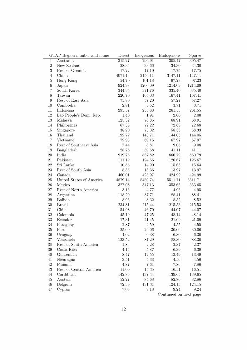
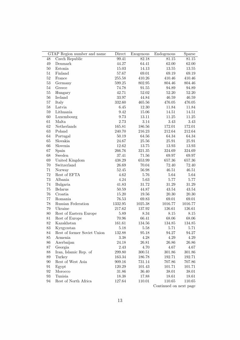
21730.77 21730.77 21730.77 21730.77Table 2: Direct carbon emissions and carbon emissions embodiedin the final demand of GTAP regions (Mt CO2).

323

Table 2 shows the comparison of the total embodied carbon in each re-324

gion, compared to direct emissions, using the three models (with the direct325

calculation method). The values shown do not include household emissions,326

which are identical in all models, and values may be different from those327

reported in Peters et al. [2011a] because we used the unprocessed GTAP328

emissions data.329

As expected, we find that the results of the endogenous dense MRIOT330

and the sparse MRIOT models are identical, apart from numerical rounding331

errors: the relative difference between the two methods is always less than332

10−4%. This is valid for the aggregate values show in Table 2 and for the dis-333

aggregate multiplier values for every sector of every region. The trade share334

allocations of the endogenous dense MRIOT and the intermediate firms of335

the sparse MRIOT play the same mathematical role, which is to distribute a336

given aggregate flow homogeneously among a certain number of disaggregate337

sectors.338

In contrast, the difference between the exogenous dense MRIOT and the339

sparse MRIOT models can be as large as 25% and has a median value of 2%.340

By term of comparison, the relative difference between direct emissions and341

the sparse MRIOT model can be as large as 81% with a median of 25%. As342

14

already noted by Peters et al. [2011a], the allocation of the provision of in-343

ternational transport to final consumption instead of its provision to a global344

pool of international transport (the difference between the exogenous and the345

sparse model) is much larger than the difference between the endogenous and346

sparse models, but much smaller than the difference between direct emissions347

and the results of the sparse model.348

5 Conclusions349

The most appropriate computational tool for a given task depends on the350

scale of the problem considered. The demands posed by the processing of a351

highly aggregated single-region closed IO table or those of a detailed multi-352

regional IO table covering the whole world are vastly different. The latter353

case involves a considerable amount of data and substantial computational354

requirements.355

The GTAP database is often used to build a world MRIOT. In this paper356

we have shown that this can be done with minimal processing, producing a357

light and fast sparse MRIOT. The gains over an equivalent dense model are of358

an order of magnitude in terms of data storage and computation time, using359

the iterative implementation, and of more than three orders of magnitude in360

terms of processing time.361

It is important to emphasize that data storage refers both to space in the362

hard disk and to active memory. Therefore, the use of the sparse MRIOT363

greatly expands the range of possibilities offered to researchers that do not364

have access to supercomputers.365

We also note that the advantage of the sparse over the dense format are366

not specific to the current size of the GTAP database. Therefore, the sparse367

format allows for a substantial increase in the size of the system (for example368

by integrating the GTAP with sub-national regional data or process-oriented369

life-cycle data). The dense format, on the other hand, is already very close370

to the computational limit posed by the RAM and cache specifications of371

modern personal computers (a few GB).372

The preparation of a MRIOT is much more time-demanding than the final373

computation, and most of that time is spent debugging code. To debug the374

code, however, requires performing the computation multiple times, which375

leads to a multiplier effect: by saving computation time, the sparse MRIOT376

also saves programming time.377

The GTAP database is already provided in sparse format, and so the con-378

version to a sparse MRIOT is particularly straightforward. However, we be-379

lieve that the use of a sparse format in the construction and analysis of a large380

15

MRIOT is convenient, whichever the data source, because in such models the381

problem of under-determined transactions always arises. The consideration382

of intermediate firms is more parsimonious than the mathematically equiv-383

alent use of trade share allocations because it avoids a substantial amount384

of data processing, which is always error-prone, and it is also conceptually385

clearer.386

In conclusion, we believe that the sparse format should be preferred over387

the dense format both due to the computational advantages and the concep-388

tual clarity that it offers in the construction and analysis of multi-regional389

input-output tables.390

Acknowledgments391

We would like to thank the financial support of FCT through grant PTDC/-392

AMB/64762/2006 and FCT and the MIT Portugal Program through schol-393

arship SFRH/BD/42491/2007 (to AM).394

16

References395

M. Brockmeier. A graphical exposition of the GTAP model. GTAP Technical396

Paper, 1996.397

S.J. Davis and K. Caldeira. Consumption-based accounting of CO2 emissions.398

Proceedings of the National Academy of Sciences, 12(107):5687–5692, 2010.399

G. H. Golub and C. F. Van Loan. Matrix Computations. John Hopkins400

University Press, Baltimore, USA, 1996. 3rd edition.401

E.G. Hertwich and G.P. Peters. Carbon footprint of nations: a global, trade-402

linked analysis. Environmental Science and Technology, 16(43):6414–6420,403

2009.404

IDE. Asian international input-output tables 2000 volume 1. explanatory405

notes. Technical report, Institute of Developing Economies, Japan External406

Trade Organization, Japan, 2006.407

M. Lenzen, K. Kanemoto, A. Geschke, D. Moran, P. Munoz, J. Ugon,408

R. Wood, and T. Yu. A global multi-region input-output time series at409

high country and sector detail. 18th International Input-Output Conference410

of the International Input-Output Association, 2010.411

B. Narayanan and T.L Walmsley. Global trade, assitance and production:412

the GTAP 7 data base. Technical report, Center for global trade analysis413

– Purdue University, West Lafayette, IN, 2008.414

J. Oosterhaven. On the plausibility of the supply-driven input-output model.415

Journal of Regional Science, 2(28):203–217, 2006.416

J. Oosterhaven, D. Stelder, and S. Inomata. Estimating international in-417

terindustry linkages: Non-survey simulations of the asian-pacific economy.418

Economic Systems Research, 20 (4):395–414, 2008.419

G.P. Peters and E.G. Hertwich. CO2 embodied in international trade with420

implications for global climate policy. Environmental Science and Tech-421

nology, 5(42):1401–1407, 2008.422

G.P. Peters, R. Andrew, and J. Lennox. Constructing an environmentally423

extended multi-regional input-output table using the GTAP database. Eco-424

nomic Systems Research, 2(23):131–152, 2011a.425

17

G.P. Peters, J.C. Minx, C.L. Weber, and O. Edenhofer. Growth in emission426

transfers via international trade from 1990 to 2008. Proceedings of the427

National Academy of Sciences, 21(108):8903–8908, 2011b.428

J. Rodrigues, A. Marques, and T. Domingos. Carbon Responsibility and429

Embodied Emissions: Theory and Measurement. Routledge, London, UK,430

2010.431

A. Tukker, E. Poliakov, R. Heijungs, T. Hawkins, F. Neuwahl, J.M. Rueda-432

Cantuche, S. Giljum, S. Moll, J. Oosterhaven, and M. Bouwmeester.433

Towards a global multi-regional environmentally extended input-output434

database. Ecological Economics, 69(7):1928–1937, 2009.435

T. Wiedmann. A review of recent multi-region input-output models used436

for consumption-based emission and resource accounting. Ecological Eco-437

nomics, 69(2):211–222, 2009.438

18