Magnetic fields - transmission lines - sag conductor
1. INTRODUCTION
The calculation and measurement of fields generated by high voltage power transmission lines has been amajor concern in the past years. Of the possible health implications and environmental impact caused by
electric and magnetic fields of high voltage electric power lines, the most difficult issue to face will often be public perceptions of the possible health hazard, specifically an increased risk of contracting cancer, caused bythe magnetic field of the power line [1-7].
Also utilities are challenged by the need to expand transmission system capacity to meet growing customerrequirements. The acquisition of new transmission Right-of-Way (ROW) is very difficult, expensive and timeconsuming due to land use public concerns. Standardization of right-of-way distances for power linessometimes include consideration of expected magnetic fields [8]. Other research has centered upon the designof power line proximity detectors, instrumentation and measurements equipment, and new line configuration.The ability to calculate magnetic fields levels that corrective with measurement data is important in all of thisinvestigation [8].
Several publications have been made to calculate and measure the electric and magnetic fields created by power transmission lines. Most assume lines parallel to a flat ground, and the sag due to the line weight isneglected [9]. One publication [8] calculated the magnetic field of a catenary line in state of single phase. Inthis paper presented method in [8], was extended not only to 3-Phase transmission lines but also to those thathave a change in direction.
1. CATENARY GEOMETRY
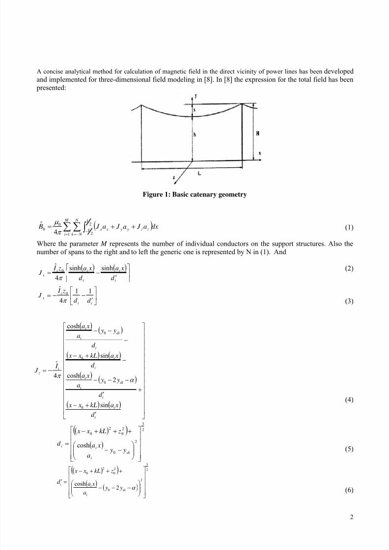
Figure 1 depicts the basic catenary geometry for a single-conductor line, where H is the maximum height onthe extremes of the line where it is anchored, h is the minimum height at mid-span (hence the sag is S=H-h)and L is the span length between adjacent towers.
A concise analytical method for calculation of magnetic field in the direct vicinity of power lines has been developedand implemented for three-dimensional field modeling in [8]. In [8] the expression for the total field has been
presented:
Figure 1: Basic catenary geometry
(1) Where the parameter M represents the number of individual conductors on the support structures. Also thenumber of spans to the right and to left the generic one is represented by N in (1). And
(2)
(3)
(4)
(5)
(6)
( )dxa J a J a J B M
i
N
N k
L
L z z y y x x∑ ∑ ∫= −=
−++=
1
2
2
00
4ˆ
π
µ
( ) ( )⎥⎦
⎤⎢⎣
⎡
′−=
i
i
i
ii
xd
xa
d
xa z I J
sinhsinh
4
ˆ0
π
⎥⎦
⎤⎢⎣
⎡′
−−=ii
i y
d d
z I J
11
4
ˆ 0
π
( )( )
( ) ( )
( )( )
( ) ( )⎥⎥⎥⎥⎥
⎥⎥⎥⎥⎥⎥⎥⎥
⎦
⎤
⎢⎢⎢⎢⎢
⎢⎢⎢⎢⎢⎢⎢⎢
⎣
⎡
′
+−
+′
−−−
−+−
−
−−
−=
i
i
i
di
i
i
i
i
i
di
i
i
i z
d
xakL x x
d
y y
a
xa
d
xakL x x
d
y ya
xa
I J
sin
2cosh
sin
cosh
4
ˆ
0
0
0
0
α π
( )( )
( )
2
3
2
0
2
0
2
0
cosh
⎥⎥⎥⎥
⎦
⎤
⎢⎢⎢⎢
⎣
⎡
⎟⎟ ⎠
⎞⎜⎜⎝
⎛ −−
+++−
=di
i
ii
y ya
xa
zkL x x
d
( )( )
( ) ( )
2
3
2
0
2
0
2
0
2cosh
⎥⎥⎥
⎥
⎦
⎤
⎢⎢⎢
⎢
⎣
⎡
⎟⎟ ⎠
⎞⎜⎜⎝
⎛ −−−
+++−
=′ α di
i
ii
y ya
xa
zkL x x
d
8/12/2019 The Influence of Conductor Sag on Spatial Distribution of Transmission Line Magnetic Field
Also the complex depth of each element of image current can be found as given in [10,11]:
(7)The parameter in (7) is the skin depth of the earth represented by
Where is the resistivity of earth and f is frequency of the source current.
3. EXAMPLES OF CALCULATIONS
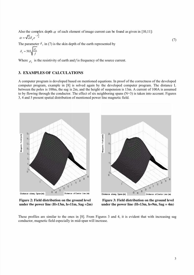
A computer program is developed based on mentioned equations. In proof of the correctness of the developedcomputer program, example in [8] is solved again by the developed computer program. The distance L
between the poles is 100m, the sag is 2m, and the height of suspension is 13m. A current of 100A is assumedto by flowing through the conductor. The effect of six neighboring spans (N=3) is taken into account. Figures
3, 4 and 5 present spatial distribution of mentioned power line magnetic field.
Figure 2: Field distribution on the ground level Figure 3: Field distribution on the ground level
under the power line (H=13m, h=11m, Sag =2m) under the power line (H=13m, h=9m, Sag = 4m)
These profiles are similar to the ones in [8]. From Figures 3 and 4, it is evident that with increasing sagconductor, magnetic field especially in mid-span will increase.
42π
δ α j
g e−
=
f
g
g
ρ δ 503=
α
gδ
g ρ
8/12/2019 The Influence of Conductor Sag on Spatial Distribution of Transmission Line Magnetic Field
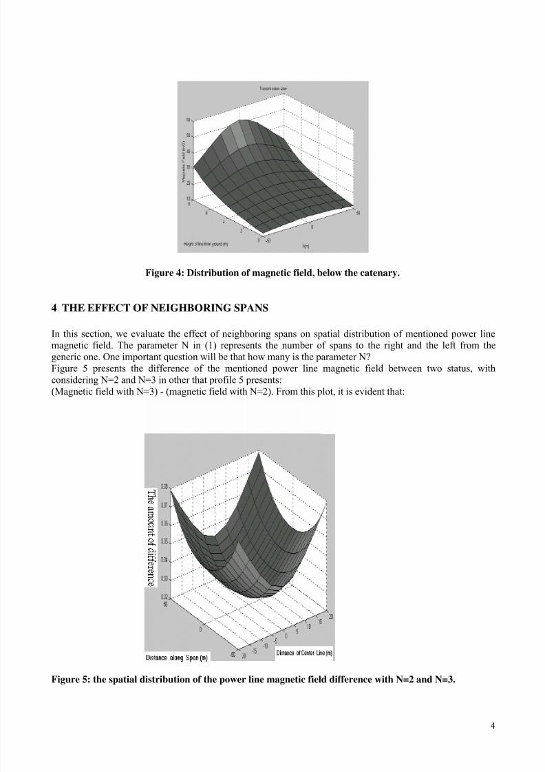
Figure 4: Distribution of magnetic field, below the catenary.
4. THE EFFECT OF NEIGHBORING SPANS
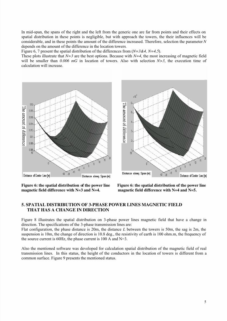
In this section, we evaluate the effect of neighboring spans on spatial distribution of mentioned power linemagnetic field. The parameter N in (1) represents the number of spans to the right and the left from thegeneric one. One important question will be that how many is the parameter N?Figure 5 presents the difference of the mentioned power line magnetic field between two status, withconsidering N=2 and N=3 in other that profile 5 presents:(Magnetic field with N=3) - (magnetic field with N=2). From this plot, it is evident that:
Figure 5: the spatial distribution of the power line magnetic field difference with N=2 and N=3.
8/12/2019 The Influence of Conductor Sag on Spatial Distribution of Transmission Line Magnetic Field
In mid-span, the spans of the right and the left from the generic one are far from points and their effects onspatial distribution in these points is negligible, but with approach the towers, the their influences will beconsiderable, and in these points the amount of the difference increased. Therefore, selection the parameter N depends on the amount of the difference in the location towers.Figure 6, 7 present the spatial distribution of the differences from ( N=3&4, N=4,5).
These plots illustrate that N=3 are the best options. Because with N=4, the most increasing of magnetic fieldwill be smaller than 0.006 mG in location of towers. Also with selection N>3, the execution time ofcalculation will increase.
Figure 6: the spatial distribution of the power line Figure 6: the spatial distribution of the power line
magnetic field difference with N=3 and N=4. magnetic field difference with N=4 and N=5.
5. SPATIAL DISTRIBUTION OF 3-PHASE POWER LINES MAGNETIC FIELD
THAT HAS A CHANGE IN DIRECTION
Figure 8 illustrates the spatial distribution on 3-phase power lines magnetic field that have a change in
direction. The specifications of the 3-phase transmission lines are:Flat configuration, the phase distance is 20m, the distance L between the towers is 50m, the sag is 2m, thesuspension is 10m, the change of direction is 10.8 deg., the resistivity of earth is 100 ohm.m, the frequency ofthe source current is 60Hz, the phase current is 100 A and N=3.
Also the mentioned software was developed for calculation spatial distribution of the magnetic field of realtransmission lines. In this status, the height of the conductors in the location of towers is different from acommon surface. Figure 9 presents the mentioned status.
8/12/2019 The Influence of Conductor Sag on Spatial Distribution of Transmission Line Magnetic Field
Figure 8: The spatial distribution of a 3-phase power lines magnetic field
that has a change in direction.
Figure 9: The layout of a real transmission line.
6. CONCLUSIONS
In this paper, calculation of magnetic fields in the direct vicinity of 3-Phase power lines that have achange in direction has been developed and implemented for three-dimensioned field modeling. The
method takes into account the sag of the conductors of power lines. Also the effect neighboring spanson spatial distribution of power line magnetic field was evaluated and discussed.
8/12/2019 The Influence of Conductor Sag on Spatial Distribution of Transmission Line Magnetic Field
[1] M. Darveniza, D. Mackerras, “ Electric and Magnetic Field Effects From Power Lines: Review of Possible
Health Effects”, Lightning and Transient Protection PTY. LTD, 1 November 2002.[2] http://www.esaa.com.org.au [3] http://www.nrpb.org.uk [4] http://www.electricity.org.uk [5] http://www.iee.org.uk [6] http://www.enertech.net [7] http://www.niehs.nih.gov/emfrapid [8] A.V.Mamishev, R.D.Nevels, B.D.Russel, “Effects of Conductor Sag on Spatial Distribution of PowerLine Magnetic Field”, IEEE Trans. On Power Delivery, Vol 11, No. 3, July 1996, pp. 1571-1576.[9] Transmission Line Reference Book, 345 kV and Above, Second Edition, EPRI Report EL-2500, EPRI,
Palo Alto, CA, 1982. [10] J.R.Wait, K.P.Spies, “On the Image Representation of the Quasi-Static Fields of a Line Current Source
Above the Ground”, Canadian Journal of Physics, Vol.47, 1969, pp.2731-2733.[11] R.G.Olsen, T.A.Pankaskie, “On the Exact, Carson and Image Theories for Wires at or Above the Earth’s
Interface”, IEEE Trans. on Power Apparatus and System, Vol.102, No.3, March 1983, pp.769-774.