THE MONETARY APPROACH TO ITS HISTORICAL EVOLUTION … · · 2015-01-27THE MONETARY APPROACH TO...

THE MONETARY APPROACH TO ITS HISTORICAL EVOLUTION AND

Thomas M. Humphrey

One of the oldest debates in economics is that between the monetary and balance of payments approaches to the determination of exchange rates in a flexible exchange rate regime. The monetary approach attributes exchange rate movements largely to actual and anticipated changes in relative money stocks. It stresses a channel of causation running from money to domestic prices to the exchange rate. By contrast, the balance of payments approach holds autonomous nonmonetary factors affecting individual items in the balance of payments to blame. It stresses a causal channel running from real factors through the balance of payments to the exchange rate and thence to domestic prices and sometimes further to the money supply. Both views underlie current discussions of the weakness of the dollar- the monetary approach holding excessive U. S. money growth to blame while the balance of payments view sees excessive oil imports and the slug- gish foreign demand for U. S. exports as the culprits. Although the difference between these two rival approaches is fairly well understood, what is not so fully appreciated is that the current debate between them is largely a repetition of earlier disputes going back more than 200 years.

The purpose of this article is to trace the emergence and development of the monetary approach in three of these early controversies, namely (1) the Swedish bullionist controversy of the 1750’s, (2) the English bullionist controversy of the early 19th cen- tury, and (3) the German inflation controversy during and immediately following World War I.1 These debates are crucial to the evolution of the monetary approach in two respects. First, they established the analytical foundations of the monetary approach. These foundations consist of a quan-

* This article draws from the author’s paper of the same title in the forthcoming volume A Monetary Approach to International Adjustment, ed. by Bluford H. Putnam and D. Sykes Wilford (New York: Praeger Publishers, 1978).

1 For another treatment of the role of the monetary and the balance of payments approaches in these debates see Johan Myhrman, “Experiences of Flexible Exchange Rates in Earlier Periods: Theories, Evidence, and a New View,” Scandanavian Journal of Economics, 78, no. 2, (1976), 169-196.

tity theory relationship linking money to prices, a purchasing power parity relationship linking prices to the exchange rate, and an expectations theory specifying how anticipations of future money stocks are formed and how they influence the exchange rate. Second, the’ earlier debates are the origin of current monetarist policy prescriptions for strengthening the dollar. These prescriptions call for the gradual de- celeration of the growth rate of the money supply so as to eliminate the excess supply of dollars alleged to be the basic cause of the fall of the internal and external value of the dollar.

The Swedish Bullion & Controversy (1755-1765:)

One of the earliest debates in which the monetary approach played a leading role was the Swedish bul lionist controversy of the mid-1700’s.2 The events precipitating the debate were as follows. In 1745 Sweden shifted from a metallic monetary system with fixed exchange rates to an inconvertible paper system with flexible exchange rates. The suspension of convertibility was followed by a steady rise in the prices of commodities and foreign exchange. A debate then arose between the two main political parties of the time-the so-called Hats and the Caps, respectively-over the cause of these price increases.

The Hat Political Party The Hats advanced the balance of payments theory, blaming both the external and the internal depreciation of the Swedish mark on Sweden’s adverse trade balance. Specifically, they held that the adverse trade balance had produced a.

depreciating exchange, that exchange depreciation had rendered imported goods more expensive, and that the rise in import prices had spread to the rest of the economy thereby raising the general level of prices. Here is an early example of the tendency of balance of payments theorists (1) to attribute both domestic inflation and exchange depreciation to external nonmonetary shocks and (2) to assert a chain of causation running from the exchange rate to prices rather than vice versa as in the monetary ap-

*On what follows, see Robert V. Eagly, The Swedish Bullionist Controversy (Philadelphia: American Philo- sophical Society, 1971).

2 ECONOMIC REVIEW, JULY/AUGUST 1978

proach. Consistent with their balance of payments view, the Hats prescribed export promotion and import restriction schemes as remedies for inflation and eschange rate depreciation. Nothing was said about money.

The Cap Party The opposition Cap party em- phatically rejected the Hats’ balance of payments theory and instead pointed to the importance of the monetary factor. They blamed both domestic inflation and the external depreciation of the Swedish mark largely on the Riksbank’s overissue of banknotes following the suspension of convertibility. They favored a policy of monetary contraction to roll back prices and the exchange rate to pre-inflation levels. Their position can be summarized by the relationship

(1) E = E(M)

expressing the exchange rate E (defined as the domestic currency price of a unit of foreign currency) as a function of the domestic money stock M.

The preceding was not tine only explanation offered by the Caps. They also adhered to an evil-speculator theory of exchange rate movements. This conspiracy theory is no part of the monetary approach. For that reason the Caps cannot be considered as full- fledged consistent advocates of -the monetary approach.

Pehr Niclas Christiernin One participant who did articulate the monetary view was Pehr Niclas Christiernin, an academic economist at the University of Uppsala, who advanced a quantity theory explanation of the transmission mechanism linking money with the exchange rate. In his Lectures on the High Price of Foreign Exchange in Sweden (1761), Christiernin maintained that the chief cause of currency depreciation was an overissue of banknotes by the Riksbank and that causation flowed from money to spending to all prices, including the prices of commodities and foreign exchange. He saw monetary expansion as stimulating demand. Part of the demand pressure falls on domestic commodity markets raising prices there. The rest spills over into the current account of the balance of payments in the form of increased demand for imports. The resulting import deficit then puts upward pressure on the exchange rate which consequently rises to restore equilibrium in the current account. Clearly, money- induced changes in total spending constitute the driving force in Christiernin’s version of the transmission mechanism running from money to the exchange rate. This component has been a hallmark of the monetary approach ever since.

As for policy recommendations, Christiernin was opposed to the Caps’ plan to restore the exchange rate to its original pre-inflation level via contraction of the note issue. His opposition stemmed from his belief that prices adjusted sluggishly in response to deflationary pressure so that the monetary contraction required to restore the exchanges to parity would bring painful declines in output and employment rather than the desired price decreases. For this reason he recommended stabilizing the exchange rate at the level established during the inflation rather than restoring it to the pre-inflation level3 Un- fortunately, his advice was ignored and the Caps enacted a deflationary policy that resulted in the very drop in output and employment that he had predicted.

The English Bullionist Controversy (1797-1819) The monetary and balance of payments theories clashed again in the famous controversy over the cause of the fall of the British pound following the Bank of England’s suspension of the convertibility of banknotes into gold during the Napoleonic wars.4 As in the earlier Swedish controversy, one side blamed currency depreciation on the central bank’s overissue of notes while the other side blamed it on an adverse balance of payments. This time, however, the proponents of the monetary and balance of payments views were known as the bullionists and the antibullionists, respectively.

The bullionists did more than any group before or since to develop and clarify the monetary view. The so-called strict bullionists crystallized the theory in rigorous form and the moderate bullionists refined and extended it. The strict bullionists included William Boyd. David Ricardo, and John Wheatley while the moderate bullionists included William Blake, Francis Horner, William Huskisson, and above all, Henry Thornton.

The Strict Bullionists: Ricardo and Wheatley The strict bullionists made several major contributions to the monetary approach. They were the first to specify both the quantity theory and purchasing power parity links in the transmission mechanism connecting money and the exchange rate. In addition, they stated the monetary approach in its most rigid and uncompromising form, asserting that, under conditions of inconvertibility where money cannot

3 Ibid, pp. 27-29, 34.

4 On the English bullionist controversy see Denis P. O’Brien, The Classical Economists (London: Oxford University Press, 1975), pp. 147-153 and Jacob Viner, Studies in the Theory of International Trade (New York: Augustus Kelley, 1965), pp. 119-170.

FEDERAL RESERVE BANK OF RICHMOND 3

drain out into foreign trade, the exchange rate varies in exact proportion with changes in the money supply. They arrived at this latter conclusion via the following route.

First, they assumed that under inconvertibility domestic prices P vary in strict proportion with the quantity of money in circulation M. This of course is the rigid version of the quantity theory which may be expressed as

(2) P = kM

where k is a constant equal to the ratio of the circulation velocity of money to real output, both treated as constants by the strict bullionists.

Second, they maintained that under inconvertibility the exchange rate E moves in proportion to the ratio of domestic to foreign prices P/P*. First enunciated by Wheatley in 1803, this proposition is the famous purchasing power parity doctrine, so christened by Gustav Cassel who rediscovered it more than 100 years later in 1918. The Wheatley-Ricardo-Cassel purchasing power parity condition may be written as

(3) E = P/P*

implying that external currency valuations derive from their real internal values and that the general price level and its counterpart, the purchasing power of money, are everywhere the same when converted into a common unit at the equilibrium rate of exchange.

Third, they assumed that the foreign price component P* of the purchasing power parity ratio was a constant equal to the given world bullion price of commodities so that exchange rate movements reflected corresponding movements in domestic paper money prices only. Given this assumption the exchange rate is a good proxy for domestic prices and may be expressed as

(4) E = P

assuming the constant foreign price level is “nor- malized” and set equal to unity.5

Finally they substituted the exchange rate proxy for the price variable in the quantity theory relationship, thereby obtaining the result

(5) E=kM

5Due to the unavailability of reliable general price in- dexes, the Classical economists also used the paper money price of bullion as an empirical proxy for the commodity price level. Accordingly, they interpreted a rise in the market price of gold above its mint price as both a sign and measure of general price inflation and therefore of the need for monetary contraction.

which states that the exchange rate varies in exact proportion with the money supply. On this basis they were able to conclude that a rise in the exchange rate above its gold parity constituted both proof and measure of overissue of inconvertible currency. In other words, if the exchange rate stood 5 percent above its gold parity, then this was prima facie evidence that the note issue was 5 percent above what it would have been under convertibility. This was most clearly stated by Ricardo who wrote

If a country used paper money not exchangeable for specie, and, therefore, not regulated by any fixed standard, the exchanges in that country might deviate from par in the same proportion as its money might be multiplied beyond that quantity which would have been allotted to it by general commerce, if . . . the precious metals had been used.6

Wheatley extended the analysis to the case where both countries are on an inconvertible paper standard. He simply substituted quantity theory rela- tionships for both the domestic and foreign price variables in Equation 3. This gave him the result that the exchange rate varies in proportion with relative money supplies, i.e.,

(6) E = kM/k*M* = K(M/M*)

where K is the ratio of the constants k and k*. Wheatley stated this result when he declared that “the course of exchange is the exclusive criterion [of] how far the currency of one [country] is increased beyond the currency of another."7

Another contribution of the strict bullionists was their assertion that exchange rate movements are purely a monetary phenomenon. They rejected the antibullionist argument that real disturbances to the balance of payments-e.g., harvest failures, wartime disruption of trade, military expenditures abroad,- were responsible for the fall of the paper pound during the Napoleonic wars. Regarding supply

shocks and foreign remittances, they denied that such factors could influence exchange rates even in the short run. Their position was that the slightest real pressure on the exchange rate would, by making British goods cheaper to foreigners, result in an instantaneous expansion of exports sufficient to eliminate the pressure. In their view, an adverse

6 David Ricardo, The Principles of Political Economy and Taxation (London: J. M. Dent and Sons, 1917), p. 151, quoted in James W. Angell, The Theory of Inter- national Prices (New York: Augustus Kelley, 1965), p. 69 n. 3. Emphasis added.

7 John Wheatley, Remarks on Currency and Commerce (London: Burton, 1803), p. 207, quoted in Angell op. cit., p. 52.


exchange was solely and completely the result of an excess issue of currency. Ricardo even went so far as to argue that even if foreign transfers and domestic crop failures did affect the exchanges by reducing real income and hence the demand for money, the cause of exchange depreciation is still an excess stock of money, albeit one arising from a reduction of money demand rather than an expansion of money supply. Ricardo’s point was simply that real factors could only affect the exchange rate through shifts in money demand not offset by corresponding shifts in money supply. In such cases the latter was to blame for exchange rate movements. The notion that all factors affecting the exchange rate must do so through monetary channels, i.e., through the demand for or supply of money, is of course central to the modern monetary approach.

Finally, the strict bullionists prescribed monetary restraint as the only cure for a depreciating currency. They held that a rise in the price of foreign exchange constituted an infallible sign that the currency was in excess and must be contracted. Ricardo even defined an excess issue in terms of exchange depreciation, thus implying a single unique correct money stock, namely one associated with the exchange being at its former gold standard parity.8

The Moderate Bullionists: Blake and Thornton

The moderate bullionists modified the strict bullionists’ analysis in three respects. First, they pointed out that it applies to long-run equilibrium situations but not necessarily to the short run. Second, while acknowledging that long-run (persistent) exchange depreciation stemmed solely from note overissue, they were willing to admit that real shocks could affect the exchanges in the short run. Their position is best exemplified by William Blake’s distinction between the Real and the Nominal exchange.” Ac- cording to Blake, the real exchange or real barter terms of trade R is determined by nonmonetary factors-crop failures, unilateral transfers, structural changes in trade and the like-that affect the balance of payments. The nominal exchange, N, however, reflects the relative purchasing powers of different currencies as determined by their relative supplies M/M*. Blake’s analysis can be summarized by the equation

(7) E = RN

that expresses the actual exchange rate as the product of its real and nominal components, both of

8 Regarding the policy implications of the Ricardian definition of excess, see O’Brien, op. cit., p. 138.

9 On Blake, see O’Brien, op. cit., pp. 150-151.

which contribute to exchange rate movements in the short run. Blake maintained, however, that in the long run the real exchange R is self-correcting (i.e., returns to its original level) and that only the nominal exchange N can remain permanently de- pressed. Therefore, persistent exchange depreciation is a sure sign of an excess issue of currency.

The third modification was made by Henry Thorn- ton, whose analysis of the money-price-exchange rate nexus was much more subtle and sophisticated than that of the strict bullionists. In particular, he argued that interest rates and the velocity of money enter the nexus, that velocity is extremely variable in the short run owing to shifts in business confidence, and that this variability invalidates the rigid money-price-exchange rate linkage postulated by the extreme bullionists.10 In terms of Equations 2 and 5 he argued that the velocity-output ratio k is a variable determined by the interest rate i and the state of business confidence c, i.e.,

(8) k = k(i, c).

Since k varies in the short run, the exchange rate and money do not exhibit exactly equiproportional movements. A given change in the money stock affects k as well as the exchange rate. In the long run, however, k is a constant and the equiproportion- ality proposition holds.

The Antibullionists Except for an expectations mechanism, the bullionists had assembled and inte- grated all the elements of the monetary theory of exchange rate determination. Compared to this ac- complishment the contributions of the antibullionists appear pretty meager indeed. They attributed exchange depreciation and domestic inflation solely to real factors-crop failures, overseas military expenditures and the like-operating through the balance of payments. They correctly asserted that the exchange rate is determined by the supply and demand for foreign exchange arising from external transactions. But they failed to see that an important factor influ- encing supply and demand might be relative price levels determined by relative money stocks. In fact, they rejected all monetary explanations, claiming that banknote expansion could not affect the exchanges in the slightest. They thought the price of foreign exchange could rise indefinitely without indicating the existence of an excess note issue. As for policy recommendations, they urged curtailment of imports and overseas expenditures to improve the balance of

10 Thornton’s contribution is discussed in O’Brien, op. cit., pp. 119-150.


payments and to strengthen the pound. They doubted that any conceivable reduction in the banknote issue could restore the exchanges to parity.

Their main analytical tool was the real bills doctrine, which they employed in an unsuccessful attempt to refute the charge that the Bank of England had overissued the currency. The real bills doctrine states that money can never be issued in excess as long as it is tied to bills of exchange arising from real transactions in goods and services. Henry Thornton, however, exposed the fallacy of this doctrine when he pointed out that rising prices would require an ever-growing volume of bills to finance the same level of real transactions. In this manner inflation would justify the monetary expansion necessary to sustain it and the real bills criterion would not effec- tively limit the quantity of money in existence. Thornton’s demonstration of the invalidity of the real bills doctrine constituted a victory for the bullionists and for the monetary approach to the exchange rate. The victory, however, was not defini- tive. For when the debate erupted again in World War I, the balance of payments approach was the dominant view.

The German Inflation Controversy (1918-1923)

The debate reopened in 1918 when Gustav Cassel used his purchasing power parity doctrine together with the quantity theory to attack the official balance of payments explanation of the wartime fall of the German mark. Whereas the policymakers blamed the currency depreciation on real disturbances to the balance of payments-e.g., obstructions to German shipping, wartime disruption of trade and the like- Cassel blamed it on excessive monetary expansion in Germany relative to that of her trading partners.

Cassel’s Critique of the Balance of Payments

Approach Cassel’s criticism of the balance of payments theory was virtually the same as that of his strict bullionist counterparts, Wheatley and Ricardo. Like them, he argued that the exchange rate is auto- matically self-correcting in response to real shocks to the balance of payments. Therefore the theory is incapable of accounting for persistent exchange rate depreciation such as that experienced by the German mark during World War I.

Regarding the operation of the self-correcting exchange rate mechanism, he noted that when balance of payments disturbances push the external value of a currency below its internal value, the currency becomes undervalued on the foreign exchanges, i.e., its domestic purchasing power is greater than indicated by the exchange rate. Such undervaluation, he held,

will immediately invoke forces returning the exchange rate to equilibrium. For as soon as a country’s currency becomes undervalued relative to its purchasing power parity, foreigners will find it prof- itable to purchase the currency for use in procuring goods from that country. The resulting increased demand for the currency will bid its price back to the level of purchasing power parity. In short, deviations of the exchange rate from purchasing power parity generate corrective alterations in the trade balance that eliminate the deviations. Both the balance of payments and the exchange rate return swiftly to equilibrium. Thus, contrary to the balance of payments view, external nonmonetary shocks have no lasting impact on the exchange rate.ll It follows that any persistent depreciation must be due to excessive monetary growth that raises domestic prices and thereby alters the purchasing power parity or equilibrium exchange rate itself. In this connection he repeated Ricardo’s dictum that an excess supply of money, whether stemming from a rise in money supply or a fall in money demand, is always and everywhere the cause of exchange rate movements.‘”

Cassel also criticized the proposition that exchange depreciation causes domestic inflation rather than vice-versa. He acknowledged that currency depreci- ations relative to purchasing power parity produce import price increases. But he denied that these import price increases could be transmitted to general prices provided the money stock and hence total spending were held in check. He maintained that, given monetary stability, the rise in the particular prices of imported commodities would be offset by compensating reductions in other prices leaving the general price level unchanged. In short, he denied that causation ran from the exchange rate to domestic prices as contended by the balance of payments approach.13

Hyperinflation and the Reverse Causality Argu- ment Despite Cassel’s forceful and vigorous attack, the debate did not go into high gear until the

post-war hyperinflation episode of the early 1920’s.14:

11 Gustav Cassel, Money and Foreign Exchange After 1914 (New York: MacMillan, 1922), pp. 149, 164-165.

12 Cassel held that drops in output and the demand for money could not affect the exchange rate if offset by corresponding equiproportional reductions in the money supply. Therefore an inappropriate money supply was to blame for exchange rate movements. Ibid., pp. 61-62, 168-169.

13 Ibid., pp. 145, 167-168.

14 What follows relies heavily on Ellis’s classic survey of the German inflation controversy. See Howard S. Ellis, German Monetary Theory, 1905-1933 (Cambridge: Har- vard University Press, 1934), Chapters 12-16.


During this episode the price of foreign exchange rose to fantastic multiples of its prewar level and everybody wanted to know why. Advocates of the monetary approach, including Cassel and his follow- ers, pointed to the explosive growth of the money supply as the obvious answer. But proponents of the balance of payments approach dismissed the monetary factor and instead attributed exchange depreciation to the adverse balance of payments caused by the burden of reparations payments combined with Germany’s alleged “fixed need for imports” and “absolute inability to export.” In their view, money had nothing to do with the fall of the mark. On the contrary, they claimed that causation ran from the exchange rate to money rather than vice-versa. They specified the following causal order of events : depreciating exchanges, rising import prices, rising domestic prices, consequent budget deficits and increased demand for money requiring an accommo- dative increase in the money supply.15

Regarding the increase in the money supply, they contended that the exchange-induced rise in prices created a need for money on the part of business and government, that it was the Reichsbank’s duty to meet this need, and that it could do so without affecting prices. Far from seeing currency expansion as the source of inflation, they argued that it was the solution to the acute shortage of money caused by skyrocketing prices. Here is the familiar argument that the central bank must accommodate supply-shock inflation in order to prevent a disas- trous contraction of the real (price-deflated) money stock. German proponents of the balance of payments view, however, pushed this argument to ridic- ulous extremes. In 1923 when the Reichsbank was already issuing currency in denominations as high as 100 trillion marks, Havenstein, the President of the Reichsbank, expressed hope that the installation of new high speed currency printing presses would help overcome the money shortage. Citing the real bills doctrine, he refused to believe that the Reichs-

15 Balance of payments theorists placed the blame for government deficits financed by new money issues squarely on inflation rather than- on the actions of the policy authorities. Inflation, they said, caused government expenditures-which were largely fixed in real terms and thus rose in step with prices-to rise faster than revenues-which were fixed in nominal terms in the short run and thus adjusted sluggishly to inflation. The result was an inflation-induced deficit that had to be financed by money growth. The authorities had nothing to do with the deficit. The monetary school rejected this argument on the grounds that the government possessed-the power to reduce its real expenditures and, moreover, that the authorities had deliberately en- gaged in deficit spending for several years prior to the hyperinflation thus establishing the monetary precondi- tions essential to that episode.

bank had overissued the currency. He also flatly denied that the Reichsbank’s discount rate of 90 percent was too low although the market rate on short term loans was an astronomical 7,300 percent per annum.16

Characteristics of the Balance of Payments School It is instructive at this point to identify the chief characteristics of the German balance of payments school if only because some of these characteristics survive in vestigial form in popular discussion of the fall of the dollar. First, members of the school tended to adhere to superficial supply and demand explanations of the exchange rate. Some merely asserted that the exchange rate is determined by supply and demand without saying what influences supply and demand. Others specified certain autonomous real factors affecting the balance of payments as the underlying determinants of foreign exchange supply and demand. None recognized that relative price levels and/or relative money stocks might also play a role. These variables were effec- tively excluded from the balance of payments school’s list of exchange rate determinants.

The school’s second characteristic was its tendency to identify exchange depreciation with one or two items in the balance of payments. In particular, members singled out raw material imports as the culprit just as some analysts currently blame petrol- eum imports. Third, they tended to treat the items in the balance of payments as predetermined and independent when in fact they are interdependent variables determined by prices and the exchange rate. For example,. they asserted that Germany’s import requirements were irreducible regardless of price and that her exports were likewise fixed. They then extended this reasoning to the other accounts of the balance of payments. Fourth, they denied the operation of a balance of payments adjustment mechanism. This denial followed from their assumption that both the balance of payments and the exchange rate are exogenously determined by factors that are independent of money, prices, and the exchange rate itself. This assumption permitted no equilibrating feedback effects from the exchange rate to the balance of payments. M. J. Bonn, a prominent balance of payments theorist, expressed the point as follows.17

Suppose, he said, that import contraction is impos-

16 Leland Yeager, International Monetary Relations: Theory, History, and Policy, 2nd edition, (New York: Harper and Row, 1976), p. 314.

17 Bonn’s views are discussed in Paul Einzig, The His- tory of Foreign Exchange (London: MacMillan, 1962), pp. 271-272, and Ellis, op. cit., pp. 248-252.


sible given Germany’s dependence on imported raw materials and foodstuffs. Likewise export expansion is impossible because of tariff barriers and economic depression abroad. Now assume a disturbance that produces a deficit in Germany’s trade balance thereby causing an exchange rate depreciation of the mark relative to its purchasing power parity equilibrium. According to Cassel and his school, the depreciation should, by lowering the foreign price of German exports and raising the domestic price of her imports, spur the former and check the latter thereby restoring equilibrium in the trade balance. But these price- induced readjustments in trade are impossible when imports and exports are independent of exchange rate changes. In such a case, an adverse trade balance may persist in the face of an undervalued currency, contrary to the conclusion of the monetary school. Finally, the fifth characteristic of the German balance of payments school was its categorical re- jection of the proposition that money influences prices and the exchange rate. As previously men- tioned, this antimonetarist view was implicit in the school’s reverse causation, money shortage, and real bills doctrines.

The Monetary School’s Critique Members of the monetary school had little trouble exposing the falla- cies in these views. They noted that supply and demand constitute only the proximate determinants of the exchange rate, that the ultimate determinants are the factors underlying supply and demand themselves, and that these factors include relative price levels determined by relative money stocks. They pointed out that the components of the balance of payments are variables not constants, that they are determined simultaneously by prices and the exchange rate, and that exchange rate movements pri- marily reflect monetary pressure on the entire balance of payments rather than nonmonetary disturbances to particular accounts. Regarding the reparations account, they noted that the depreciation of the mark was not caused by these payments per se but rather by the inflationary way they were financed, i.e., by fresh issues of paper money. As for Ger- many’s alleged need for a fixed physical quantity of imports regardless of price, they argued that needs are not incompressible and that even the import demand for absolute necessities possesses some price elasticity. Moreover, they pointed out that exports too are responsive to changes in relative prices and that the exchange rate mechanism would therefore tend to equilibrate exports and imports were it not continually frustrated by inflation. They maintained that had domestic prices stopped rising, a further

depreciation of the mark would, by making German goods cheaper to foreigners and foreign goods dearer to Germans, have stimulated exports and re- strained imports until a new equilibrium was reached. In their view, it was only the rise in domestic prices consequent upon the increase in the money supply that prevented the expansion of exports and the contraction of imports. Otherwise current account equilibrium would have been restored by the exchange- induced shift in the relative prices of exports and imports.

Most important, advocates of the monetary approach argued convincingly that exchange depreciation originated in excessive money growth and that the monetary authorities could have stopped the depreciation had they been willing to exercise control over the money stock. In short, they showed that the price of foreign exchange could not have risen indefinitely unless sustained by inflationary money growth. Had the latter ceased, the exchange rate would have stabilized.

The Expectations Element The German inflation controversy contributed the last of the three major elements to the monetary approach. The English bullionist writers had already established the quan tity theory and purchasing power parity elements. All that remained was the statement and development of the expectations theory linking anticipations of future money supplies with the current exchange rate. This step was taken during the hyperinflation debate when the monetary school sought to explain why the dollar/mark exchange rate actually rose faster than the German money supply. According to the strict quantity theory and purchasing power parity hypotheses, the two variables should rise at roughly the same rate. Their failure to do so was taken by the balance of payments school as consti- tuting evidence of the invalidity of the monetary approach. Advocates of the monetary approach, however, rescued it from this criticism by explaining the exchange rate-money growth disparity in terms of market expectations. In a nutshell, they contended that in disequilibrium the exchange rate is influenced by the expected future exchange rate (i.e., the anticipated purchasing power parity) which depends on prospective price levels governed by expected money stocks. Howard Ellis, in his German Monetary Theory 1905-1933 (1934), cites several economists, notably Gustav Cassel, Walter Eucken, Fritz Machlup, Ludwig von Mises, Melchior Palyi, A. C. Pigou, and Dennis Robertson, who claimed that exchange rate movements reflected anticipated increases in the money stock and who argued that


the external value of the mark varied in proportion to the expected future quantity of money rather than to the actual current quantity. In sum, observers watching the money supply accelerate month after month naturally came to expect future money growth to exceed present money growth and these expectations caused the exchange rate to outpace the money

supply. Similar explanations were advanced to account for

disparities between the rate of domestic price inflation and the rate of currency depreciation in Ger- many. Eucken, Machlup, and von Mises argued that the exchange rate embodies inflationary expectations and that exchange rate movements parallel movements in expected future prices, not actual current prices. For this reason, they claimed, the exchange rate may deviate from the purchasing power parity computed from current price levels. Cassel perhaps put the matter most clearly when he wrote that

A depreciation of currency is often merely an expression for discounting an expected fall in the currency’s internal purchasing power. The world sees that the process of inflation is continually going on, and that the condition of State finances, for instance, is rendering a continuance of the depreciation of money probable. The international valuation of the currency will, then, generally show a tendency to anticipate events, so to speak, and becomes more an expression of the internal value the currency is expected to possess in a few months, or perhaps in a year’s time.18

As this passage suggests, members of the monetary school not only explained how expectations affect the exchange rate, but also how expectations themselves are determined. In essence, they said that people base their exchange rate expectations on observations of the behavior of the policy authorities, especially the latter’s monetary and fiscal response to large budgetary commitments like reparations payments. These observations yield information about the authorities’ policy strategy which people use in predicting future policy actions affecting the exchange rate. As Dennis Robertson put it in his famous

textbook Money (1922), “. . . the actual rate of exchange is largely governed by the expected behavior of the country’s monetary authority . . ."19

In the case of Germany, the authorities were already demonstrating a pronounced tendency to finance reparations payments with budget deficits and excessive monetary growth. People expected this policy to continue in the future and these expectations were embodied in the exchange rate.20

Conclusion This article has surveyed the development of the monetary approach to the exchange rate in three historical controversies with the rival balance of payments approach. The article offers some support for Sir J. R. Hicks’s argument that monetary theory, unlike other branches of economic theory, tends to be influenced by historical events and episodes, notably severe monetary disturbances and institutional changes that alter the character of the monetary system.21 In the case of the monetary theory of the exchange rate, at least, Hick’s argument seems validated. For, as discussed above, the main elements of the monetary approach emerged from controversies triggered by currency, price, and exchange rate upheavals following the suspension of metallic parities. Specifically, the article argues that the monetary approach originated in the Swedish bullionist controversy of the 1750’s, that its quantity theory and purchasing power parity components were thoroughly established during the English bullionist controversy of the early 1800’s, and that the expectations component was added during the German inflation debate of the early 1920’s. Thus all the elements of the modern monetary approach were firmly in place by the mid-1920’s.

19 Dennis Robertson, Money (London : Cambridge Uni- versity Press, 1922), p. 133.

20 Expectations were not the only factor cited by the monetary school as causing the exchange rate to lead prices and money. Another was currency substitution, i.e., the substitution of stable dollars for unstable marks in German residents’ transactions and asset money bal- ances.

21 Sir John Hicks, Critical Essays in Monetary Theory (London: Oxford University Press, 1967), pp. 156-158. l8 Cassel, op. cit., pp. 149-150.


SEASONAL MOVEMENTS IN SHORT-TERM YIELD SPREADS Thomas A. Lawler

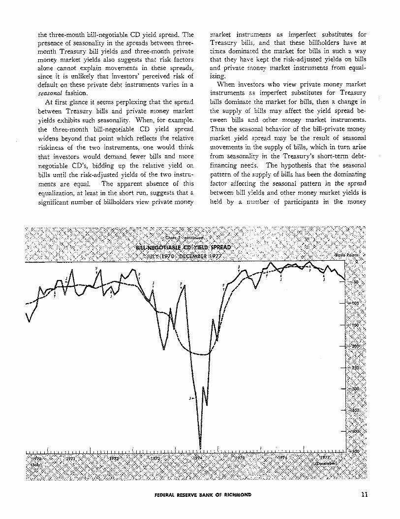
One of the more interesting aspects of the behavior of short-term interest rates over the past 15 years has been the volatilty of the spread between the yield on Treasury bills and the yield on private money market instruments. One such spread, the difference between the three-month Treasury bill yield and the yield on three-month large negotiable certificates of deposit (CD’s) traded in the New York secondary market, ranged from 3 basis points to over 400 basis points during the 1963 to 1977 period. (All yields referred to in this paper are bond-equivalent yields.) The volatility of this spread, which is shown in Chart 1, appears, at least on an intuitive basis, to be much greater than can be attributed to changes in the relative riskiness of bills and negotiable CD’s

Analysis of the three-month Treasury bill-negotiable CD yield spread indicates that it is subject to seasonal variation. Chart 1, which also plots a centered 12-month moving average of the spread, reveals a definite seasonal pattern in the yield spread series. For example, the Treasury bill-negotiable CD yield spread in February lies above its corresponding 12-month moving average in every year save one, and for 11 of 14 years the June yield spread is below its moving average. Moreover, in all but two of the fifteen years from 1963 to 1977 the June Treasury bill-negotiable CD yield spread was below the Febru- ary yield spread. Analysis of the three-month bill- prime bankers acceptance and three-month bill- prime commercial paper yield spreads reveals that they exhibit seasonal movements similar to that of


the three-month bill-negotiable CD yield spread. The presence of seasonality in the spreads between three- month Treasury bill yields and three-month private money market yields also suggests that risk factors alone cannot explain movements in these spreads, since it is unlikely that investors’ perceived risk of default on these private debt instruments varies in a seasonal fashion.

At first glance it seems perplexing that the spread

between Treasury bills and private money market

yields exhibits such seasonality. When, for example,

the three-month bill-negotiable CD yield spread

widens beyond that point which reflects the relative

riskiness of the two instruments, one would think

that investors would demand fewer bills and more

negotiable CD’s, bidding up the relative yield on

bills until the risk-adjusted yields of the two instru-

ments are equal. The apparent absence of this

equalization, at least in the short run, suggests that a

significant number of billholders view private money

market instruments as imperfect substitutes for Treasury bills, and that these billholders have at times dominated the market for bills in such a way that they have kept the risk-adjusted yields on bills and private money market instruments from equal- izing.

When investors who view private money market instruments as imperfect substitutes for Treasury

bills dominate the market for bills, then a change in

the supply of bills may affect the yield spread be-

tween bills and other money market instruments.

Thus the seasonal behavior of the bill-private money

market yield spread may be the result of seasonal

movements in the supply of bills, which in turn arise

from seasonality in the Treasury’s short-term debt-

financing needs. The hypothesis that the seasonal

pattern of the supply of bills has been the dominating

factor affecting the seasonal pattern in the spread

between bill yields and other money market yields is

held by a number of participants in the money


market.10 The hypothesis states that a seasonal increase in the supply of Treasury bills causes bill yields to be bid up relative to private money market yields, and a seasonal decrease in the supply of bills results in bill yields being bid down relative to private money market yields. Consequently, evidence indicating that seasonal movements in the supply of bills are positively related to seasonal movements in the spread between bill yields and private money market yields would tend to support the hypothesis that investors who consider private money market instruments as imperfect substitutes for Treasury bills have been dominating the market for bills, at least in the short run.

This paper examines the relationship between seasonal movements in the three-month Treasury bill- negotiable CD yield spread and seasonal movements

1 For example, see Salomon Brothers, Comments on Credit, March 31, 1978.

in the amount of Treasury bills outstanding. In the first section the seasonal components of the two series are analyzed. The second section deals with some of the reasons why certain investors may consider instruments such as negotiable CD’s and prime: commercial paper as imperfect substitutes for Trea- sury bills. Finally, the last section discusses some of the implications of the analysis.

Seasonal Movements in Treasury Bills Outstand- ing and in the Bill-Negotiable CD Yield Spread

Treasury Bills Outstanding The multiplicative version of the Bureau of the Census’ X-11 seasonal adjustment program was used to estimate the monthly seasonal component of the amount of Trea- sury bills outstanding.2 The series used measures

2 For a description of the X-11 program see [9]. For a less technical description, as well as a discussion of some of the shortcomings of the X-11, see Lawler [5].


the par value of Treasury bills maturing within one year that are held by private investors at the end of each month.3 The solid line in Chart 2 represents the monthly X-11 seasonal factors obtained for this series from 1963 to 1977. The chart shows that the amount of Treasury bills held by private investors has exhibited a recurring intrayear pattern, with the amount of bills outstanding falling on average from February to June as Federal tax revenues rose relative to expenditures, and increasing on average from September to February as tax revenues fell relative to expenditures.

Three-Month Treasury Bill-Negotiable CD Yield Spread The monthly seasonal component of the spread between the three-month Treasury bill yield and the three-month negotiable CD yield was esti-

3 That is, Treasury bills held by Federal government agencies and the Federal Reserve are excluded.

mated by using the additive version of the X-11 seasonal adjustment program. Since the additive version assumes that the seasonal component equals the difference between the original series and the seasonally-adjusted series, the seasonal factors for the bill-negotiable CD yield spread series are measured in basis points. The dashed line in Chart 2

plots the monthly X-11 seasonal factors obtained for the three-month Treasury bill-negotiable CD yield spread series from 1963 to 1977. The chart indicates that on average the spread has tended to rise from September to February and decline from January to June.

Comparison Chart 2 also illustrates the remark- able similarity between the seasonal pattern of the three-month Treasury bill-negotiable CD yield spread and the seasonal pattern of the amount of bills outstanding. The chart shows that, on average, both series have tended to peak in February, fall from

FEDERAL RESERVE RANK OF RICHMOND 13

February to June, and rise from September to Febru- cording to the chart, the major change in the shape

ary. It should be noted that seasonal movements in of the seasonal pattern of bills outstanding over the

the two series do not coincide exactly. This is not ten year period was that the amount of bills out-

surprising, since the bills outstanding series is an standing declined on average from July to Septem-

end-of-month series, while the yield spread series is a ber during the 1973 to 1977 period, while in the

monthly average series. On the whole, however, earlier period the amount of bills outstanding in-

Chart 2 suggests that there is indeed a positive rela- creased seasonally from July to September. The

tionship between seasonal changes in the amount of chart also shows a similar change in the seasonal

bills outstanding and seasonal movements in the bill- pattern of the three-month Treasury bill-negotiable

negotiable CD yield spread. CD yield spread.

Closer examination of Chart 2 also reveals that

changes in the shapes of the two seasonal patterns

over time are related. Chart 3 compares the average

estimated seasonal factors of the two series for the

1963 to 1967 period with the average seasonal factors of the two series for the 1973 to 1977 period. Ac-

The seasonal pattern in yield spreads, moreover,

is not limited to the spread between Treasury bill

yields and negotiable CD yields. Chart 4 plots the

average X-11 seasonal factors for the three-month

Treasury bill-prime commercial paper yield spread

for the 1963-1967 and 1973-1977 periods as well as


the average seasonal factors for the amount of bills outstanding for these two five-year periods.4 The chart illustrates that the seasonal pattern of the Trea- sury bill-commercial paper yield spread is quite similar to that of bills outstanding and that of the bill- negotiable CD yield spread.

4 The three-month prime commercial paper rate used here is that for high-grade prime commercial paper quoted by Salomon Brothers [7]. The commercial paper yield for each month is the average of the yield for the first day of the month and the yield for the first day of the following month. Since the Treasury bill yield series employed is a monthly average of daily yields, the different averaging procedures may cause this bill-commercial paper yield spread series to be more volatile. There is no reason, however, why the different averaging procedures themselves should cause the yield spread series to exhibit either seasonal or cyclical movements.

The similarity of the seasonal patterns of Treasury bills outstanding and the spread between bill yields and private money market yields suggests that short- run changes in the supply of bills have affected the yield on bills relative to the yield on other money market instruments. This implies that investors who are insensitive to the differential yields of Treasury

bills and other money market instruments have in-

deed at times dominated the market for bills, at least

in the short run. The next section examines possible

reasons for such investor behavior, as well as who

these investors might be.

Determinants of the Substitutability of Treasury Bills and Private Money Market Instruments Investors manage their portfolios in such a way that the risk-adjusted return on the marginal dollar of


each asset held is equal to that on the marginal dollar of all other assets held. Optimal portfolio behavior does not, however, necessarily imply that the pecuniary risk-adjusted market yields on all assets held will be equal. For example, investors hold demand deposits even though the pecuniary yield on such deposits is zero. The reason demand deposits are held, of course, is that they provide nonpecuniary returns to the investor in the form of safety, conveni- ence, liquidity, and the like.

The relative risk-adjusted pecuniary yields on any two debt instruments of the same maturity may not reflect their implicit relative returns to a given investor for a number of reasons.5 For one thing, one debt instrument may provide services not adequately measured by its explicit market yield and not provided by other instruments. Additionally, the markets for different debt instruments may be such that the minimum denomination of one instrument is much larger than that of another instrument, and wealth constraints may limit an investor’s choice of investments to those debt instruments below the minimum denomination of one but not another instrument. Finally, legal constraints may prohibit certain investors from holding one instrument but not another instrument.

Commercial banks constitute an investor group for which Treasury bills provide services not provided by private money market instruments. Banks in most states are required to pledge certain assets equal to a set percentage (typically 100 percent) of their state and local deposits, and Treasury bills are acceptable pledging assets in all states while private debt instruments are almost never acceptable.6 Fur- ther, thirty states allow banks outside of the Federal Reserve System to hold some fraction of their reserve requirements in Treasury bills, while only a few states allow any private debt instruments to fulfill part of a bank’s reserve requirements.’ Finally, bank regulators often judge a bank’s capital adequacy by its ratio of equity to risky assets, where the latter are defined as total assets less cash and U. S. Government securities. Therefore a bank may hold Treasury bills simply to maintain this capital adequacy ratio and thus appease its regulators.8 For these and other reasons, a bank’s demand for Trea- sury bills may be sizable even when the explicit yield

5 This discussion assumes that there are no technical factors such as differential tax treatment affecting short- term yield spreads.

6 See Gilbert and Lovate [3].

7 See Haywood [4].

8 See Summers [8].

differential between bills and private money market instruments exceeds that corresponding to their relative riskiness.

A group for whom wealth constraints have limited the substitutability of Treasury bills and private money market instruments consists of small investors. The minimum denomination of negotiable CD’s is $100,000, and commercial paper, while sometimes issued in units as small as $25,000, is usually traded in the money market in lots of $100,000 face value. Treasury bills, on the other hand, are issued in denominations as small as $10,000. Consequently, a number of small investors have been able to purchase Treasury bills but have been unable, due to wealth constraints, to purchase negotiable CD’s and commercial paper.

Finally, state and local governments’ holdings of Treasury bills have been fairly insensitive to bill- private money market yield spreads because a number of state statutes allow these governments to hold Treasury bills but not commercial paper or out-of- state CD’S.9 A number of foreign official institutions face similar constraints in that their holdings of U. S. securities are limited by regulation to Treasury securities such as bills.

These examples do not comprise an all-inclusive list of those investors whose demand for bills is inelastic with respect to the bill-private money market yield differential. They do illustrate, however, that there exist a large number of billholders whose demand for bills is relatively insensitive to these yield spreads. On the other hand, there are a number of investors whose demand for bills is quite sensitive to yield differentials. Consequently, the question of whether a change in the supply of bills results in a change in the relative yield on bills and. other instruments is an empirical one. The evidence presented in this paper supports the hypothesis that: changes in the supply of bills have affected the spread between bill yields and private money market yields, at least in the short run. It should be realized, however, that past dominance of the bill market by investors who view private money market instruments as imperfect substitutes for Treasury bills does not imply that they will dominate the bill market in the future. Indeed, the emergence of money market funds, which pool individual investors’ funds to purchase money market instruments, suggests that small investors’ holdings of Treasury bills will be more sensitive to the spread between bill yields and private money market yields than they have been in the past.

9See [1].


Further, the recent change in Regulation Q allowing banks and savings and loan associations to issue small ($10,000) floating-rate six-month certificates of deposit whose yield is tied to the six-month Trea- sury bill rate now provides small investors with a close substitute for bills. Thus, it is difficult to determine what effect, if any, short-run changes in the supply of Treasury bills will have on the yield spread of bills and private money market instruments in upcoming years.

Implications The Treasury bill rate is often used as an overall indicator of credit market conditions. If, as seems to be the case, bill yields rise or fall relative to private money market yields as the supply of bills changes, then it is questionable whether the monthly bill rate actually reflects the general price of credit. The problems with using the bill rate as a short-run credit market indicator may not be trivial,

as the average estimated seasonal change in the three- month Treasury bill-negotiable CD yield spread during the 1970’s from seasonal peak to seasonal trough is almost 50 basis points.

Further, if supply factors can affect bill-private money market yield spreads, then changes in the demand for Treasury bills of investors who view private money market instruments as imperfect sub-

stitutes for bills should also have affected these yield

spreads. For example, the huge amount of bills

purchased by small investors during the 1973-74

period of disintermediation, as well as the large pur-

chases of bills by foreign central banks over the last

year to help support the dollar, may have affected

the spread between bill yields and private money

market yields during these periods. Thus, caution is

advised in using the Treasury bill rate as a histori-

cal measure of the short-run general price of credit.

References

1. Advisory Commission on Intergovernmental Rela- tions. Understanding State and Local Cash Man-

5. Lawler, Thomas A. “Seasonal Adjustment of the

agement. Washington, D. C., Government Printing Money Stock : Problems and Policy Implications.”

Office (May 1977). Economic Review, Federal Reserve Bank of Rich- mond (November/December 1977), pp. 19-27.

2. Cook, Timothy Q. “Limited Habitats, Required Habitats, and Preferred Habitats : the Determinants of Short-Term Yield Spreads.” Unpublished manu- script, Federal Reserve Bank of Richmond, 1978.

3. Gilbert, R. Alton, and Lovate, Jean M. “Bank Re- serve Requirements and Their Enforcement: A Comparison Across States.” Review, Federal Re- serve Bank of St. Louis (March 1978), pp. 22-32.

4. Haywood, C. F. The Pledging of Bank Assets: A Study of the Problem of Security for Public De- posits. Association of Reserve City Banks, Chicago

6. Salomon Brothers. Comments on Credit, various issues.

7. An Analytical Record of Yields and Yield Spreads. New York (1977).

8. Summers, Bruce. “Bank Capital Adequacy: Per- spectives and Prospects.” Economic Review, Federal Reserve Bank of Richmond (July/August 1977), pp. 3-8.

9. U. S. Department of Commerce, Bureau of the Census. The X-11 Variant of the Census Method II Seasonal Adjustment Program, by J. Shiskin, A. H. Young, and J. C. Musgrave. Technical Paper No. 15, Washington, D. C.: 1967.


LIFO INVENTORY ACCOUNTING: EFFECTS INVENTORY-SALES RATIOS, AND

Walter A. Varvel

Changes in the rate of inventory investment have played an important role in the pattern of economic growth in the current recovery that began in early 1975. Though inventory investment accounts for only a small portion of gross national product, changes in the rate of activity in this sector have often dominated the influence exerted by all other components (final sales) of GNP on quarterly economic growth rates. Table I compares growth rates of inflation-adjusted GNP, real final sales, and changes in the rate of inventory investment over the last ten quarters. The dominant role of inventory investment is especially evident in each of the first and fourth quarters shown in the table. Reductions in the rate of change in business inventories in the fourth quarters of 1975, 1976, and 1977, respectively, have overshadowed strong gains in final sales and significantly moderated economic growth in those quarters. Conversely, increases in inventory building in the first quarters of 1976, 1977, and 1978 offset concurrent slowdowns in sales and led to higher GNP growth rates than would be indicated from total sales figures alone. Inventory behavior, therefore,

Table I

INVENTORY INVESTMENT, REAL FINAL SALES,

AND REAL GNP

Change In Inventory Inventory Real Final

Investment1 Investment1 Sales2 Real GNP2

1975 IV - 4.6 - 7.5 +5.6 +3.0

1976 I + 9.7 +14.3 + 3.9 +8.8 II +12.1 + 2.4 +4.3 +5.1 III +13.8 + 1.7 +3.3 +3.9 IV - 1.8 -15.6 +6.3 +1.2

1977 I + 9.7 +11.5 +3.8 +7.5 II +13.2 + 3.5 +5.1 +6.2 Ill + 15.7 + 2.5 +4.4 +5.1 IV + 8.7 - 7.0 +6.1 +3.8

1978 I +14.7 + 6.0 -1.7 0.0

1 Billions of 1972 dollars, annual rate.

2Quarter-to-quarter compounded annual rates of change, 1972 dollars.

Source: Department of Commerce, Bureau of Economic Analysis.

has been watched carefully as an indicator of prospective changes in aggregate economic output.

According to the generally accepted view, the most important factor affecting business demand for inventory stocks is the expected rate of business sa1es.l When sales are expected to increase, firms generally increase their accumulation of inventories. A slowdown in expected sales, on the other hand, usually

leads to a slowdown in inventory investment. The ratio of inventories to sales (I/S), consequently, is frequently used by managers and economic analysts as a rough measure of the adequacy of business inventories relative to the level of sales. Chart 1 shows the historical relationship between book value inventories to sales ratios since 1960 for the manufacturing sector separately and for all manufacturing and trade combined. Each series suggests that fairly lean inventory stocks were maintained in 1977 relative to sales levels (i.e., I/S ratios appeared to be below

historical averages). This knowledge would seem to support expectations that inventories may increase relative to sales in the near term.

This article describes a recent significant shift in accounting methods used to value business inventories that has been encouraged by the severe inflation of the 1970’s. In an effort to remove inflation- related inventory profits from corporate profit statements, businesses have increasingly taken advantage of an industry accounting option granted 40 years ago. The switch from FIFO (first in-first out) and other related inventory accounting methods to LIFO (last in-first out) eliminates unrealized inventory profits and appears to be a rational response by business to an inflationary environment.

The switch to LIFO accounting, however, has also resulted in a change in the manner in which a portion of ending inventories are reported on corporate balance sheets. Inflation causes LIFO inventories to be biased downward and this problem is exacerbated as LIFO usage increases. Present aggregate inventories may be understated, therefore, upsetting the

1 For a discussion of the determinants of inventory investment and its influence on gross national product, with special reference to the present business cycle, see [18] and references cited in that paper.


historical comparability of I/S ratios. The article then examines whether explicit recognition of inventory accounting techniques used by business enriches understanding of recent quarter-to-quarter inventory swings. Before these effects of the LIFO method of inventory accounting are discussed, however, the impacts LIFO and FIFO have on corporate profit statements and balance sheets, respectively, are first described and the economic incentives for a switch to LIFO are explored.

FIFO and LIFO Defined FIFO and LIFO have substantially different ways of allocating inventories purchased over time at different prices to corporate balance sheets and income statements. FIFO accounting charges the cost of the first, or earliest, inventory acquired against current revenue for purposes of measuring corporate profits. Because of this, it is referred to as a historical cost accounting technique. During inflationary times the cost of

goods sold, therefore, often reflects the lower inventory prices experienced in earlier periods. The cost of the unsold (most recently acquired) inventory is carried forward to the next accounting period. FIFO

inventories on balance sheets, therefore, are valued at price levels prevailing relatively near the time when accounts are closed.

The LIFO inventory valuation method exactly reverses the FIFO treatment of inventories. The last, or most recent, inventory costs incurred are charged against current revenue in profit reports of firms using LIFO. These costs approximate the replacement cost of inventory sold during the period. Cost of goods sold with LIFO, therefore, is based on the advanced prices of inventory most recently purchased. Ending inventories on balance sheets are carried at the (lower) acquisition costs of earlier periods. Some LIFO inventories could conceivably remain on balance sheets perpetually.

From the above, it is clear that the inventory valuation method a business chooses can affect both its reported profit and stock of inventory during periods when prices are changing. During a severe inflation, as experienced in this decade, FIFO reports lower cost of goods sold and, therefore, higher profits than the LIFO accounting method. The entire difference, however, is attributable solely to inventory price changes and is generally referred to as inventory


profits. In an effort to eliminate inventory profits, many businessmen have shifted inventories to the LIFO method. The next section will briefly discuss inflation’s impact on corporate profits and will look at the potential adjustment provided by a mass shift to LIFO.

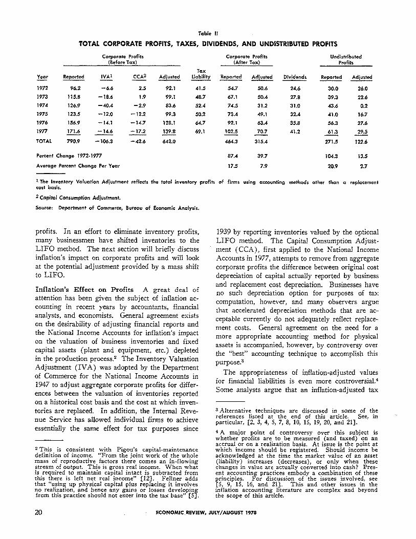
Inflation’s Effect on Profits A great deal of attention has been given the subject of inflation accounting in recent years by accountants, financial analysts, and economists. General agreement exists on the desirability of adjusting financial reports and the National Income Accounts for inflation’s impact on the valuation of business inventories and fixed capital assets (plant and equipment, etc.) depleted in the production process.2 The Inventory Valuation Adjustment (IVA) was adopted by the Department of Commerce for the National Income Accounts in 1947 to adjust aggregate corporate profits for differences between the valuation of inventories reported on a historical cost basis and the cost at which inventories are replaced. In addition, the Internal Reve- nue Service has allowed individual firms to achieve essentially the same effect for tax purposes since

2 This is consistent with Pigou’s capital-maintenance definition of income. “From the joint work of the whole mass of reproductive factors there comes an in-flowing stream of output. This is gross real income. When what is required to maintain capital intact is subtracted from this there is left net real income” [12]. Fellner adds that “using up physical capital plus replacing it involves no realization, and hence any gains or losses developing from this practice should not enter into the tax base” [5].

1939 by reporting inventories valued by the optional LIFO method. The Capital Consumption Adjust,- ment (CCA), first applied to the National Income Accounts in 1977, attempts to remove from aggregate corporate profits the difference between original cost depreciation of capital actually reported by business and replacement cost depreciation. Businesses have no such depreciation option for purposes of tax computation, however, and many observers argue that accelerated depreciation methods that are acceptable currently do not adequately reflect replacement costs. General agreement on the need for a more appropriate accounting method for physical. assets is accompanied, however, by controversy over the “best” accounting technique to accomplish this purpose.3

The appropriateness of inflation-adjusted values for financial liabilities is even more controversial4 Some analysts argue that an inflation-adjusted tax

3 Alternative techniques are discussed in some of the references listed at the end of this article. See, in particular, [2, 3, 4, 5, 7, 8, 10, 15, 19, 20, and 21].

4 A major point of controversy over this subject is whether profits are to be measured (and taxed) on an accrual or on a realization basis. At issue is the point at which income should be registered. Should income be acknowledged at the time the market value of an asset (liability) increases (decreases), or only when these changes in value are actually converted into cash? Pres- ent accounting practices embody a combination of these principles. For discussion of the issues involved, see [5, 9, 15, 16, and 21]. This and other issues in the inflation accounting literature are complex and beyond the scope of this article.


system must recognize as taxable income the accrued capital gain on the decline in the real value of net corporate debt caused by inflation [e.g., see 1, 16, 21]. Inflation adjustment of financial liabilities has not received as much attention as adjustments for physical assets and no allowance for debt revaluation is presently incorporated or required in the National Income Accounts or corporate income statements.

Table II gives the Commerce Department’s estimates of the overstatement of corporate profits due to inflation since 1972.5 Total corporate profits before and after taxes are shown along with official estimates of adjustments necessary for inventory profits and underdepreciation of fixed capital. Ac- cording to these figures, inventory profits and underdepreciation led to an overstatement of corporate profits for tax purposes by $150 billion over the last six years. The IVA corrects for over two-thirds of this total overstatement although underdepreciation has become the larger factor over the last three years. Subtraction of dividends paid to stockholders from after-tax profits reveals that the burden of the inflation distortion is borne by retained earnings.6 This burden is actually understated by the figures in Table II, which are in current dollars and, therefore, do not reflect the erosion of the purchasing power of these funds.

In effect, then, inflation raises the tax burden on business, depriving investors of the ability to recover the real value of used-up physical capital without being taxed on that recovery. Fellner, Clarkson, and

5 These figures include no attempt to adjust the value of corporate debt for inflation.

6 Inclusion of an estimate of reduction in real indebted- ness due to inflation, it has been claimed, reduces the overstatement of internally generated funds in corporate accounts [21].

Moore feel inflation introduces “unlegislated taxation of capital” and “reduces the incentive to invest” [6, p. 3]. The combined effects of inflation, namely, increasing effective tax rates on capital7 and the erosion of an important source of funds available for investment, therefore, have adversely affected business investment in recent years.

Table III shows that the experience of nonfinancial companies has been even worse than that evidenced for all corporations. Excluding financial companies, the greatest distortion in business profits occurred in 1974 when inflation hit double-digit levels. For that year alone, after-tax profits and retained earnings of nonfinancial companies were overstated by $43.3 billion. In 1974, nonfinancial companies actually paid out in taxes and dividends more than their realized earnings.

The LIFO accounting method yields adjustments in reported earnings equivalent in size to the IVA when physical inventories are increased or unchanged and something less than the IVA when physical inventories are liquidated.8 The size of the IVA and the behavior of aggregate real business inventories suggests the application of LIFO accounting to all inventories could perhaps have reduced reported aggregate corporate profits by as much as $90-$100 billion over the 1972-1977 period. Proportionate reductions in taxes and dividends paid could have

7 Considerable evidence has been presented that supports the view that the net effect of inflation has been that the annual net return on capital, defined as the sum of inflation-adjusted profits and the actual net interest paid, has been subject to higher effective corporate income tax rates the higher the rate of inflation [e.g., 6, 11, and 20].

8 When physical stocks decline during an inflationary period, an IVA is required also for a portion of inventories valued on a LIFO basis, since some inventories sold are not carried at replacement cost but in terms of prices of prior periods [13].


significantly improved actual cash flow. Corpora- tions, it appears, had a powerful incentive, therefore, to utilize the LIFO option during the last several inflation-plagued years.

The Switch to LIFO A significant increase in the use of LIFO inventory accounting has, in fact, taken place in recent years. The Department of Commerce estimates that the proportion of total manufacturing inventories valued on a LIFO basis doubled in 1974 and has stabilized at approximately 33 percent since that time.” Table IV shows the results of an annual survey of inventory valuation methods used by 600 major U. S. companies. Over 50 percent of these companies used LIFO for some portion of their inventories in 1974, more than twice the number reporting LIFO usage in prior years. This proportion has increased slightly since 1974. Nevertheless, many firms do not make use of LIFO at all and most who do only apply it to a portion of their inventories. The interesting question, in light of the apparently large tax-saving and liquidity benefits accruing to LIFO users, though, is why the large majority of firms still value inventories with accounting methods that do not remove the effect of inventory price changes. Apparently, other considerations have limited the switch from FIFO to LIFO.

LIFO’s Disadvantages There are several con- sequences of using LIFO that appear unattractive to management thereby prompting firms to retain usage of historical cost methods of inventory accounting. Perhaps the most important consequence is that earnings per share reported by LIFO firms are usually lower than they would be through alternative accounting methods. Per share earnings or earnings on total assets remain important performance yardsticks for management and stockholders. LIFO accounting may lead to smaller dividends to stockholders and smaller bonuses and salary increases to corporate management since each are usually tied to profit performance. Management, as well as owners, therefore, may be reluctant to switch to LIFO unless the firm has a strong underlying liquidity need.

Secondly, LIFO’s potential benefits to individual firms may be reduced or even eliminated during periods when inventory prices are falling. Certainly, on an aggregate basis, inventory prices have risen uninterruptedly in the 1970’s. Some materials and

9 Source: John C. Hinrichs, U. S. Department of Com- merce, Bureau of Economic Analysis. In inflation adjusted terms, the figure is probably now in excess of 40 percent [141].

commodities (e.g., agricultural products), however,

have been subject to large declines in price at times. In the case of falling inventory prices, LIFO charges the lower priced items to cost of goods sold-resulting in higher profits, higher taxes, and less cash flow than FIFO accounting.10 In brief, the use of LIFO during times when inventory prices are falling may overstate taxable profits, thereby increasing tax liabilities at a time the firm can least afford it.

A third factor perhaps limiting the potential benefits of LIFO to some individual companies is oper- ational when inventories are liquidated. When inventories are being drawn down and LIFO is used, cost of goods sold include some inventory purchased and carried on the firm’s accounts at earlier (lower) prices. LIFO would still report lower profits and, therefore, result in tax savings and an improved realized cash position compared to FIFO when inventories are liquidated. The discrepancy between reporting methods, however, is reduced in this situation. The incentive to switch to LIFO is partially reduced, therefore, for firms carrying excessive inventories.

Management presumably weighs the pluses and minuses of alternative accounting techniques and assesses their likely impacts on firm operations. Though LIFO has obviously reduced tax liabilities and improved cash flow for many firms in the inflationary 1970’s, it does not necessarily follow that all firms would be similarly benefited. In addition, the adverse impact LIFO has on reported profitability is apparently judged by many firms to be too high a. price to pay far improved corporate liquidity. These

10 This situation could result in an inverse relationship between sales and reported profits. If sales increased to the point where higher-priced inventory began to be used up, these additional sales would actually produce lower profits if the product price fell with the cost of inventory. Only if inventories are liquidated would the resultant capital losses on inventory stocks be realized. Conversely,. when inventory inflation exists, inventory liquidation is a prerequisite to the realization of capital gains on inventory stocks.


firms, accordingly, have decided not to switch to LIFO.

Impact of a Switch to LIFO on Ending Inven- tories and I/S Ratios The method by which inventories are valued affects the reported book value of inventory stocks and, thus, I/S ratios. Since I/S ratios are sometimes used by managers and analysts as a measure of the adequacy of inventories relative to the level of sales, recognition of the accounting impact is essential. Sales reflect current period prices

while the book value of ending inventory can report either earlier, lower prices (LIFO) or more current, higher prices (FIFO). LIFO accounting would report lower inventories and I/S ratios than FIFO with the same size of physical inventories. During an inflationary period, therefore, LIFO results in a downward bias in I/S ratios.

The impact a switch from FIFO to LIFO will have on the value of ending inventories depends on the following factors: (a) the rate of inventory price change, (b) the percentage of total inventories valued on a LIFO basis, (c) the length of time LIFO has been used, and (d) the change in the physical stock of inventories.

Regarding the first of these factors, LIFO and FIFO will report identical inventory stocks in a non-inflationary environment. If inventory has not experienced price increases, the book value of inventories and I/S ratios will not differ whether FIFO or LIFO is used. This would be true for individual firms or for the aggregate economy. Periods of price stability, however, have not been evident in recent years. As prices rise, other things remaining constant, LIFO accounting results in relatively smaller reported inventory stocks and, therefore, smaller I/S ratios than FIFO. The greater the inflation experienced, the larger will be the discrepancy between accounting methods.

The proportion of total business inventories valued using LIFO also affects the book value of reported inventories. Given inventory price inflation, the larger the percentage of LIFO inventories, the greater the downward bias in the I/S ratio. It follows, therefore, that if a significant portion of aggregate inventories are switched from FIFO to LIFO, the divergence is enlarged following the switch. This will adversely affect the direct comparability of inventory levels and aggregate I/S ratios over time.

The length of time LIFO accounting has been used for a portion of inventories is another factor that complicates comparisons of I/S ratios over time. With inventory inflation, the discrepancy in reported

inventories between FIFO and LIFO is cumulative. Some LIFO inventories may continue to be carried at purchase prices prevailing several years earlier. Those inventories will differ from replacement cost in relation to inventory price increases experienced in each of the intervening years.

Finally, the change in physical inventories during the period affects reported inventory stocks and I/S ratios. If inventory stocks are increasing or remain unchanged, physical inventories do not turn over and LIFO inventories may reflect inventory prices incurred several years earlier. Only if inventory

stocks are being liquidated are some of the low price LIFO inventories removed from balance sheets. FIFO inventories are not affected in this manner.

A shift in inventory accounting methods alone, therefore, can result in sizable differences in reported inventories across several inflationary years. Table V illustrates the magnitude of the effect of a change in inventory accounting on reported inventories of a sample of department stores that maintained dual inventory records from 1940-1947.” The average annual reduction in ending inventories due to LIFO accounting was 4.6 percent. Further, the use of

11 This was a period of serious inflation, comparable to the 1970’s.


LIFO resulted in a 27 percent cumulative reduction in the book value of inventories over the eight-year period. Although the proportion of inventories valued by LIFO in this sample is considerably higher than presently applicable to the business sector as a whole, the example clearly illustrates the extent to which a switch to LIFO can alter the book value of inventories over time.

The exercise presented in Table VI cautions against the intertemporal comparison of I/S ratios when LIFO accounting is used for an increasing proportion of inventories. The inventories switched from FIFO to LIFO in 1974 alone are estimated to have reduced corporate profits by $9 bil1ion.12 This repre- sented approximately 3.4 percent of total business inventories that year. Assuming total inventories using LIFO doubled in 1974 (as they did in the manufacturing sector, see footnote 9), a rough estimate of the annual downward bias resulting from LIFO use prior to 1974 might approach three percent if inventory price increases were comparable. Table VI, however, is constructed assuming that the inventories already carried under LIFO prior to 1974 necessitate an annual upward adjustment of 1 percent in reported inventories to remove the downward bias in I/S ratios that LIFO inventories cause in an inflationary period. Similarly, following the switch to LIFO in 1974, a 2 percent annual adjustment in inventories is assumed necessary for 1975 1977.13

Reported I/S ratios, shown in Chart 1 and Table VI, suggest that businessmen were maintaining fairly lean levels of inventories relative to sales in 1977 when compared to earlier years. The table reveals, however, that the adjusted series describes an en- tirely different situation. Adjusted I/S ratios are, in fact, considerably higher than in 1972-1974. This exercise suggests that recently reported levels of business inventories may not be as lean as historical comparisons of unadjusted I/S ratios indicate. The last column in Table VI also shows a different pic- ture from unadjusted ratios when all inventories and sales are reported in constant 1972 dollars.14 Com-

12 John C. Hinrichs, U. S. Department of Commerce, Bureau of Economic Analysis.

13 These assumed adjustments are for demonstration purposes only and do not claim to exactly adjust I/S ratios for LIFO’s effects. The adjustments are thought to be conservative estimates, however. Smaller adjustments in 1972-1973 and 1975-1977 than 1974 reflect lower rates of inflation,

14 The first and last columns do not report identical figures for 1972 because some inventories under column 1 are reported using lower (pre-1972) inventory prices while sales are in 1972 dollars.

parisons of unadjusted I/S ratios over extended periods, therefore, should be interpreted with caution following the switch to LIFO accounting.

FIFO, LIFO, and Inventory Investment Recog-

nition of the increased proportion of business inventories valued using LIFO, in addition, may contribute to understanding the large swings in inventory investment that have occurred in the first and fourth quarters of recent years. Undoubtedly, the recent quarterly pattern of sales (strong in fourth quarters, relatively weak in first quarters) has been a prime determinant of the pattern of inventory investment. Larger-than-expected fourth quarter sales might lead to an involuntary reduction in inventory stocks in the same quarter. Conversely, weaker-than-expected first quarter sales might result in involuntary inventory building.15 Financial considerations that are affected by inventory accounting decisions, however, may also affect the decision to invest in inventories.

This section will examine whether any financial incentive is present that may induce firms to alter their quarterly inventory investment pattern. Table VII presents the operation of a hypothetical firm with. three alternative assumptions concerning changes in. inventories.16 In addition, in each case the statements, are presented using FIFO and LIFO inventory valuation for comparison. The firm is assumed to have revenue of $200 from the sale of 10 product units and a beginning inventory of 8 units valued at $64. Increases in the cost of inventory are assumed

15 Some firms apparently use LIFO only in the fourth quarter. For the remainder of the year they report monthly inventory stocks using the FIFO method. This may contribute to the swing in inventory investment from quarter to quarter [14].

16 Table VII assumes the firm has no production costs other than purchasing inventory.


to occur during the period. Three different levels of inventory purchases are assumed : (I) seven units, reducing ending inventory to five units, (II) ten units, leaving ending inventory unchanged at eight units, and (III) twelve units increasing ending inventory to ten units. Within this framework, the impact of FIFO and LIFO accounting on ending inventory, cost of goods sold, profit, taxes, and cash flow can be examined.

Table VII demonstrates that FIFO allocates the

highest cost inventories to ending inventory in the

balance sheet and the lowest cost inventories are

charged against revenues in the income statement.

LIFO allocates inventories in reverse manner, with high cost inventories applied to cost of sales and the low cost inventories remaining in ending inventory. Consequently, in each case of assumed inventory purchases, ending inventories and I/S ratios are smaller with LIFO than with FIFO. Conversely, the cost of sales is larger with LIFO than with FIFO. In each instance, reported profits and taxes using FIFO are higher than those using LIFO. A portion of FIFO profits, however, are tied up in inventory and the cash is not available unless inventories are liquidated. The higher taxes paid on these inventory profits result in a less favorable cash flow position for the firm if it uses FIFO inventory valuation compared with the use of LIFO. It is in this respect that LIFO is claimed to more accurately

reflect profits available for distribution as dividends or to be put into retained earnings.

With FIFO inventory accounting, the firm’s reported profits and taxes are not altered by the inventory purchase decisions depicted in Table VII. Its end-of-period cash position, however, is significantly improved by limiting its inventory investment-at least until after the statement closing date. This action may be necessary, for instance, to pay dividends to stockholders.

Greater flexibility is provided the LIFO user. Both profits and cash flow improve as the firm limits inventory purchases. A LIFO firm desiring to maximize reported earnings, reward shareholders with sizable dividends, and/or in need of internally generated cash would have a strong incentive to limit inventory investment. On the other hand, the firm could reduce its tax liability by additional investment in inventories, although this action would reduce reported profits and cash flow.

Inventory behavior, therefore, affects the cash position of the firm under both accounting methods. FIFO firms with end-of-year cash needs could, in part, satisfy those requirements by limiting inventory investment. A similar incentive is present for LIFO firms, although, at any given level of physical inventory, cash flow is already enhanced by the use of LIFO itself. LIFO firms are provided an extra incentive for limiting inventory, however-improve-


ment in reported profitability. It may be expected, then, that LIFO firms are especially likely to post- pone inventory purchases until after financial statement closing dates. The incentives to limit inventory stocks, of course, would not induce a firm to reduce inventories to the point where sales were adversely affected by shortages.

The switch to LIFO inventory accounting, by reducing taxes, has generated additional cash flow for American business. To gain perspective on the relative magnitude of this potential boost to cash flow, it is contrasted with the gain resulting from a reduction in the corporate income tax rate to 45 percent from the hypothetical 50 percent applied in Table VII. Using case II (where physical inventory levels are unchanged), the tax rate reduction reduces taxes and increases after-tax profits by approximately 10 percent while it increases retained earnings by approximately 38 percent ($26 to $35.80). This is considerably less than the firm’s percentage gain in cash from switching from FIFO to LIFO (from $26 to $44, almost 70 percent) .17 LIFO

17 The results of comparisons between tax rate reductions and a switch to LIFO are highly dependent on assumptions concerning the firm’s operation and the inventor? inflation it faces. The comparison results in the text are for demonstration purposes only and should not be generalized.

reduces effective corporate taxes by approximately

24 percent in this case. Since LIFO reduces before-

tax profits, it reduces taxes and increases cash flow

for the individual firm to a greater extent than a

small reduction in the corporate tax rate.

Summary Though the “best” method for infla-

tion-adjusting corporate financial statements is a

controversial topic, business presently can (if it so

chooses) eliminate inflation-related inventory profits

during inflationary periods. Though LIFO may not

be attractive to all firms, most firms can reduce tax

liabilities and significantly improve corporate cash

flow through its use. Potentially, a major switch to

LIFO accounting could result in a larger gain in

retained earnings and might provide a bigger boost

to business investment than a modest reduction in

the corporate income tax rate. Examination of other

effects of a switch to LIFO accounting suggests that

it renders intertemporal comparisons of inventory-

sales ratios hazardous and may increase the quarter-

to-quarter variability of inventory investment. Fail-

ure to recognize these effects may impair forecasts of

inventory investment and, therefore, GNP.

References

1. Aaron, H. “Inflation and the Income Tax.” The American Economic Review, (May 1976), pp. 193-

2. Baxter, W. T. “Accountants and Inflation.” Lloyds Bank Review, (October 1977), pp. l-16.

3. Cost Accounting Standards Board. “Adjustment of Historical Depreciation Costs for Inflation.” Proposed Standard No. 413, October 9, 1975.

4. Fabricant, S. Toward Rational Accounting In An Era of Unstable Money, 1936-1976. Report No. 16, National Bureau of Economic Research, December 1976.

5. Fellner, W. “Comments on Inflation Accounting and Nonfinancial Corporate Profits : Phvsical Assets.” Brookings Papers on Economic Activity, (3: 1975), pp. 599-604.

6. ; Clarkson, K.; Moore, J. Correcting Taxes for Inflation. Domestic Affairs Study 34, American Enterprise Institute for Public Policy Research, June 1975.

7. Financial Accounting Standards Board. “Proposed Statement of Financial Accounting Standards, Financial Reporting in Units of General Pur- chasing Power.” ber 1974.

FASB Exposure Draft, Decem-

8. Fox, H., and Lang, F. “Lifo’s Charms and Harms.” Quarterly Review of Economics and Business, (2: 1975), pp. 36-45.

9. Gramlich, E. “Comments on Inflation Accounting and Nonfinancial Corporate Profits : Physical Assets.” Brookings Papers on Economic Activity, (3 : 1975), pp. 604-608.

10. Neal, A. “Immolation of Business Capital.” Har- vard Business Review, (March-April 1978)) pp.

75-82

11. Nordhaus, W. “The Falling Share of Profits.” Brookings Papers on Economic Activitu. (1: 1974). pp. 169-217.

-I .

12. Pigou, A. “Maintaining Capital Intact.” Econo- mica, (August 1941), p. 271.


13. Rottenberg, I. “Inventories and the InventoryValuation Adjustment.” Quarterly GNP EstimatesRevisited in a Double-Digit Inflationary Economy,BEA Staff Paper No. 25, U. S. Department ofCommerce, Bureau of Economic Analysis, Octo-ber 2, 1974, pp. 29-33.

14. ; M. Foss; and G. Fromm. “Improvingthe Measurement of Business Inventories.” Amer-ican Statistical Association Proceedings, 1977, pp.

15. Shoven, J., and Bulow, J. “Inflation Accountingand Nonfinancial Corporate Profits : PhysicalAssets,” Brookings Papers on Economic Activity,(3: 1975), pp. 557-611.

16. . “Inflation Accounting and Nonfinan-cial Corporate Profits: Financial Assets and Lia-bilities.” Brookings Papers on Economic Activity,(1: 1976), pp. 15-66.

17. Stevenson, J. Methods of Inventory Valuation andTheir Effect on Balance Sheets and OperatingStatements, Submitted to the Graduate School ofBanking conducted by the American Bankers Asso-ciation, Rutgers University, June 1952.

18. Tatom, J. “Inventory Investment in the RecentRecession and Recovery.” Review, Federal ReserveBank of St. Louis, (April 1977), pp. 2-9.

19. Touche Ross and Co. Current Value Accounting,Economic Reality in Financial Reporting, A Pro-gram for Experimentation, 1975.

20. van Furstenberg, G. “Corporate Taxes and Finan-cing Under Continuing Inflation.” ContemporaryEconomic Problems. Edited by W. Fellner. Ameri-can Enterprise Institute for Public Policy Research,1976, pp. 225-54.

21. , and Malkiel, B. “Financial Analysisin an Inflationary Environment.” The Journal ofFinance, (May 1977), pp. 575-92.

The ECONOMIC REVIEW is produced by the Research Department of the Federal Reserve Bank ofRichmond. Subscriptions are available to the public without charge. Address inquiries to Bank andPublic Relations, Federal Reserve Bank of Richmond, P. O. Box 27622, Richmond, Virginia23261. Articles may be reproduced if source is given. Please provide the Bank’s Research Depart-ment with a copy of any publication in which an article is used. Also note that microfilm copies ofthe ECONOMIC REVIEW are available for purchase from University Microfilms, Ann Arbor, Mich-igan 48106. The identification number is 5080.


Date post:	25-Apr-2018
Category:	Documents
Upload:	phamliem
View:	217 times
Download:	3 times

THE MONETARY APPROACH TO ITS HISTORICAL EVOLUTION … · · 2015-01-27THE MONETARY APPROACH TO...

Documents