THE THEORY OF SCALE RELATIVITY ∗ LAURENT NOTTALE CNRS, D´ epartement d’Astrophysique Extragalactique et de Cosmologie, Observatoire de Paris-Meudon, F-92195 Meudon Cedex, France Received 18 April 1991 Revised 26 September 1991 Abstract Basing our discussion on the relative character of all scales in nature and on the explicit dependence of physical laws on scale in quantum physics, we apply the principle of relativity to scale transformations. This principle, in combination with its breaking above the Einstein-de Broglie wavelength and time, leads to the demonstration of the existence of a universal, absolute and impassable scale in nature, which is invariant under dilatation. This lower limit to all lengths is identified with the Planck scale, which now plays for scale the same role as is played by light velocity for motion. We get new scale transformations of a Lorentzian form and generalize the de Broglie and Heisenberg relations. As a consequence the high energy length and mass scales now decouple, energy and momentum tending to infinity when resolution tends to the Planck scale, which thus plays the role of the previous zero point. This theory solves the problem of divergence of charge and mass (self-energy) in electrodynamics, implies that the four fundamental couplings (including gravitation) converge at the Planck energy, improves the agreement of GUT predictions with experimental results, and allows one to get precise estimates of the values of the fundamental coupling constants. 1 Introduction Since the Galilean analysis about the nature of inertial motion, the theory of relativ- ity has been developed by extending its application domain to coordinates systems involved in more and more general states of motion: this was partly achieved in Einstein’s special and general theories of relativity. Hence the principle of general relativity states that “the laws of physics must be of such a nature that they apply to systems of reference in any kind of motion” [1]. However, as pointed out by Levy-Leblond, [2] the abstract principle of relativity should be distinguished from any of its possible realizations as concrete theories of relativity. This point of view may still be generalized into a framework in which * International Journal of Modern Physics A, Vol. 7, No. 20 (1992) 4899-4936. c World Scientific Publishing Company. Version complemented by notes and errata (15 May 2003). 1
Transcript
THE THEORY OF SCALE
RELATIVITY∗
LAURENT NOTTALE
CNRS, Departement d’Astrophysique Extragalactique et de Cosmologie,
Observatoire de Paris-Meudon, F-92195 Meudon Cedex, France
Received 18 April 1991
Revised 26 September 1991
Abstract
Basing our discussion on the relative character of all scales in nature andon the explicit dependence of physical laws on scale in quantum physics, weapply the principle of relativity to scale transformations. This principle, incombination with its breaking above the Einstein-de Broglie wavelength andtime, leads to the demonstration of the existence of a universal, absolute and
impassable scale in nature, which is invariant under dilatation. This lowerlimit to all lengths is identified with the Planck scale, which now plays forscale the same role as is played by light velocity for motion. We get newscale transformations of a Lorentzian form and generalize the de Broglie andHeisenberg relations. As a consequence the high energy length and mass scalesnow decouple, energy and momentum tending to infinity when resolution tendsto the Planck scale, which thus plays the role of the previous zero point.This theory solves the problem of divergence of charge and mass (self-energy)in electrodynamics, implies that the four fundamental couplings (includinggravitation) converge at the Planck energy, improves the agreement of GUTpredictions with experimental results, and allows one to get precise estimatesof the values of the fundamental coupling constants.
1 Introduction
Since the Galilean analysis about the nature of inertial motion, the theory of relativ-ity has been developed by extending its application domain to coordinates systemsinvolved in more and more general states of motion: this was partly achieved inEinstein’s special and general theories of relativity. Hence the principle of generalrelativity states that “the laws of physics must be of such a nature that they applyto systems of reference in any kind of motion” [1].
However, as pointed out by Levy-Leblond, [2] the abstract principle of relativityshould be distinguished from any of its possible realizations as concrete theories ofrelativity. This point of view may still be generalized into a framework in which
relativity is considered as a general method of thinking in sciences [3]: it consistsin analysing how the results of measurements and (cor)relations between them aredependent on the particular conditions under which the measurements have beenperformed. Assuming that these results are measured in some “reference system”(e.g. coordinate systems in case of position and time measurements), these condi-tions may be characterized as “states” of the reference systems.
Such states of reference systems play a special role in physics: they being definedas characteristics of the reference systems themselves, no absolute value can beattributed to them, but only relative ones, since they can be defined and describedonly with respect to another reference system. Two systems at least are needed todefine them. As a consequence the transformation laws between reference frameswill be of the greatest importance in a relativity theory.
In such a frame of thinking, the most fundamental relativity is the relativity ofpositions and instants. It is usually expressed in terms of homogeneity and isotropyof space and uniformity of time and actually makes up the basis of the whole ofphysics. It states that there is no preferential origin for a coordinate system and isfinally included in special relativity through the Poincare group.
Then Einstein’s relativity is, strictly, a theory of “motion relativity”, since theparticular relative state of coordinate systems which the special and general theoriesof relativity have extensively analysed (in the classical domain) is their state ofmotion.
We suggest in this paper that scale (i.e. resolution with which measurementshave been performed) may also be defined as a relative state of reference systems,and that Einstein’s principle of relativity can be generalized by requiring that thelaws of physics apply to any systems of coordinates, whatever their state of scale.In other words, we shall require scale covariance of the equations of physics. Thequantum behavior of microphysics may to some extent be reinterpreted as a man-ifestation of scale relativity. But in its present form quantum field theory corre-sponds, rather, to a Galilean version of such a scale relativity theory, especially inthe renormalization group approach.
Indeed we first recall how the renormalization group may be applied to space-time itself, yielding an anomalous dimension1 for space and time variables. Then wedemonstrate in a general way that the principle of relativity alone, in its Galileanform (i.e. without adding any extra postulate of invariance), is sufficient to derivethe Lorentz transformation as a general solution to the (special) relativity problem.Once applied to scale, and owing to the fact that physical laws become explicitelyscale-dependent only for resolutions below the de Broglie length and time (namely,that scale relativity is broken at the de Broglie transition), this reasoning leads tothe existence of an absolute, universal scale which is invariant under dilatationsand so cannot be exceeded. Then, after having identified this scale as the Planckscale, we attempt to develop a theory based on this new structure: the Einstein-deBroglie and Heisenberg relations are generalized, and first implications concerningthe domain of high energy physics are considered.
1This dimension is ‘anomalous’ in the sense that it cannot be obtained from simple dimensionalanalysis. It is actually a ‘scale dimension’, defined as the difference between the fractal dimensionand the topological dimension. It becomes a variable in scale-relativity, identified with a fifthdimension that we have called ‘djinn’ in subsequent papers.
2
2 The Dependence on Scale of Microphysics
Starting from the Planck/Einstein work at the beginning of the century, the devel-opment of the quantum theory has forced physicists to admit that the microscopicworld behaves in a radically new way compared to the classical way. One of the mainproperty of microphysics irreducible to being classical is described by the Heisenbergrelations, which imply a profound scale dependence of physical laws in the quan-tum domain. When ∆p ≫ p0 (i.e. ∆x ≪ λdB, the de Broglie length), p becomesof the order of ∆p and the position-momentum Heisenberg relation ∆p . ∆x ≈ ~
becomes p ≈ ~/∆x. Similarly when ∆E ≫ E0 (i.e. ∆t ≪ τdB, the de Broglietime), E becomes of the order of ∆E and the time-energy Heisenberg relation∆E . ∆t ≈ ~ becomes E ≈ ~/∆t. In the presently best accepted interpretationof quantum mechanics, this behaviour is understood as a consequence of the un-controllable interaction between the measurement apparatus and the system to bemeasured. However it is remarkable that the Heisenberg relations are universal andindependent from any particular measurement process. They may be derived fromthe general law that the momentum probability amplitude and position probabilityamplitude are reciprocal Fourier transforms.
So we have proposed a different interpretation [3]: that the quantum behaviouris a consequence of a fundamental and universal dependence of space-time itself onresolution, which is revealed in any measurement: namely, that the quantum space-time has fractal properties. This leads to the view that scale should be explicitelyintroduced into the fundamental laws of physics, and that this goal may be achievedby identifying it as a state of the reference system (i.e. of measurement apparatusin the language of quantum mechanics). In this frame of thought, the Heisenbergrelations tell us that the results of measurements of momentum and energy arerelative to the state of scale of the reference system.
The scale dependence of microphysics has already taken on reinforced impor-tance in the study of the asymptotic behaviour of quantum field theories, presentlybest described by the renormalization group methods [4]-[8], which led to someimportant results, like asymptotic freedom of QCD, the variation of coupling con-stants with scale and their convergence at the “Grand Unified Theory” scale ≈ 1015
GeV. These methods have for the first time explicitly introduced scale into physicalequations. Indeed it is remarkable that below the Compton length of the electron,there is a strong “degeneration” of space and time variables: the velocity becomesdisqualified as a pertinent mechanical variable (all velocities are close to the velocityof light) and the classical laws of mechanics are actually replaced by dilatations interms of Lorentz γ factors. Then, at high energy, the laws of scale actually take theplace of the laws of motion.
There are, however, several additional elements in our proposal with respect tothe standard renormalization group approach. The first is that it is argued thatscale, like motion, may be considered as a state of coordinate systems which cannever be defined in an absolute way, and thus comes under a relativity theory. Inthis respect we may identify the theory of the renormalization group as a Galileanversion of scale relativity. The second is that the renormalization group is, strictly,only a semi-group (one integrates the small scales to get the larger ones) [9], whileone may hope it to be completed in the future by an inverse transformation, at leastfor some elementary physical systems. This would mean being able to deduce the
3
small scale structure from the larger scale: this is exactly what a fractal generatormakes [3, 10, 11]. The third new element is that the relativistic analysis of scale,once applied to space and time variables themselves, finally leads to a completelynew structure of physical laws, as will be demonstrated in the following.
3 Galilean Scale Relativity
One of the main characteristics of scale which point toward the need for a scalerelativity theory is the nonexistence of an a priori absolute scale. Just as one maywrite for velocities in Galilean motion relativity :
v = v2 − v1 = (v2 − v0) − (v1 − v0), (1)
one may, in present physics, write for a scale ratio
=∆x2
∆x1=
∆x2/∆x0
∆x1/∆x0. (2)
It is indeed clear that one can never define the length of an object withoutcomparing it to another object: only scale ratios, i.e. dilatations, have a physicalmeaning. The expression (2) may be written under the same additive group formas Eq. (1), in a logarithmic representation:
ln = ln
(
∆x2
∆x1
)
= ln
(
∆x2
∆x0
)
− ln
(
∆x1
∆x0
)
. (3)
So the “scale state” V = ln(∆x2/∆x1) appears like a “scale-velocity” or “zoom”,in agreement with our principle that it should describe the state of resolution ofthe coordinate system in the same way as the velocity describes its state of motion.Just as one can speak only of the velocity of a system relative to another one, thescale of a system can be defined only by its ratio to the scale of another system.Eq. (3) may now be written in exactly the same form as Eq. (1):
V = V2 − V1 = (V2 − V0) − (V1 − V0). (4)
Concerning the problem of units, notice the difference of status between motionand scale laws. While velocity is expressed in terms of a physical unit (e.g. m.s−1),the scale state is expressed in terms of a mathematical unit, i.e. the adoptedlogarithm base. Indeed the same behaviour is obtained (whatever base b is) usingthe more general definition:
V =ln(∆x2/∆x1)
ln b= logb
(
∆x2
∆x1
)
. (5)
It will be seen hereafter that this leads to a new kind of dimensional analysis.Consider now a field ϕ which transforms under a dilatation q = ∆x/∆x′ follow-
ing a power law:ϕ′ = ϕ qδ. (6)
In a renormalization group description, the power δ is identified with the anomalousdimension of the field ϕ [9]. In a fractal interpretation of the same phenomenon, we
4
get δ = D−DT , where D is the fractal dimension and DT the topological dimension[3, 11].
We are particularly interested here in the case where the “field” ϕ is space-timeitself. Let us briefly remind the present state of things concerning this approach [3].Assume that we consider a system having first a de Broglie length λ0 = ~/p0, andthat we perform successive measurements at given time intervals with a resolution∆x in order to determine its velocity and then its average momentum and the lengthof its trajectory. If ∆x ≫ λ0, the momentum perturbation implied by Heisenberg’srelation is ∆p ≪ p0, so that the result will remain ≈ p0, independent of scale. Onegets the usual classical trajectory whose length does not depend on resolution. Onthe contrary when ∆x ≪ λ0, ∆x . ∆p ≈ ~ implies that the measured momentum willkeep practically no trace of the initial one, i.e. ∆p ≫ p0 so that p = p0 + ∆p ≈ ∆p;finally the momentum will be a direct function of resolution, p ≈ ~/∆x, and thenew de Broglie length of the system after the measurement becomes of the orderof ∆x. The length of the particle path now diverges as ∆x−1 [12, 13, 3]. Thismeans that the length L, integrated along the (fractal) path of a particle, divergesfor resolutions ∆x smaller than the de Broglie length (or time) λ as
L = L0λ
∆x, (7)
corresponding to the particular case δ = D − DT = 1 for D = 2 and DT = 1.The same behaviour is found for the temporal coordinate around the de Broglie
time of the system [3]. This result is obtained when one takes into account not onlythe transition to relativistic velocities, but also particle-antiparticle pair creations.Owing to the fact that the whole set of virtual pairs contribute in the self-energyof a particle (say, of the electron) and then in the nature of the particle itself,and extending the Feynman-Wheeler-Stuckelberg interpretation of antiparticles asparticles which run backward in time, we have suggested that, if one wants tocompute the full proper time T elapsed on the particle, one must add the propertimes elapsed on all the members of the virtual pairs to that of the “bare” particle.Thus one finds a temporal coordinate diverging with energy, i.e. in an equivalentway with the inverse of time resolution when ∆t < τ = ~/E as
T = T0τ
∆t. (8)
A similar result is obtained from localized solutions of the Dirac equation: fromthe requirement that the solution should be localized into an interval ∆x ≈ c∆t ≈~c/E, one may compute the rate of negative and positive energy solutions. Onefinds P−/P+ ≈ (E − mc2)/(E + mc2). Then considering that this set of positiveand negative solutions is nothing but the manifestation of a fractal trajectory whichruns backward in time for ∆t < τ leads to (8). This makes Lorentz covariant thereinterpretation of the de Broglie scale as a universal space-time transition fromδ = 0 to an anomalous dimension δ = 1, since it applies to all four space-timecoordinates. In terms of the renormalization group, the de Broglie scale may beidentified as the correlation length of space-time.
Keeping all these results in mind, let us write Eq. (6) in a linear form by passingonce again to a logarithmic representation:
ln
(
ϕ′
ϕ0
)
= ln
(
ϕ
ϕ0
)
+ δ × ln
(
∆x
∆x′
)
, (9)
5
this being assumed to hold when ∆x ≪ λ. Our comparison with motion relativitymay then be pursued. The Galilean transform between two coordinate systemsreads
x′ = x + vt, (10)
t′ = t. (11)
We may now get a consistent description in which, as conjectured, resolutionacts as a “scale-velocity”, while the anomalous dimension (i.e. here the fractaldimension minus 1) plays the role of a “scale-time”. Indeed, setting
X = ln
(
ϕ
ϕ0
)
, (12)
from the linear relation
X = X0 + δ × ln
(
λ
∆x
)
, (13)
we may define the state of scale V as
V = ln
(
λ
∆x
)
=d(ln ϕ)
dδ=
dX
dδ, (14)
in the same way as the velocity of an object is defined as u = dx/dt in motionrelativity. Note the different approach with respect to the usual definition for thefractal dimension δ = ∂ lnϕ/∂ ln(λ/∆x).2 The scale law (13) is the equivalent forscale of free motion at constant velocity, which is at the basis of the definition ofinertial motion. Likewise we suggest that a coordinate supersystem [3] (i.e. definedby its states of motion and of scale) into which Eq. (13) holds, may be called“scale-inertial”, and that we may set a principle of (special) scale relativity, whichstates that the laws of nature are identical into all scale-inertial supersystems ofcoordinates.
The anomalous dimension δ is assumed to be invariant (e.g. for space-timecoordinates we find the universal value δ = 1, itself coming from the universalityof the Heisenberg relations: in that case, δ is a constant), as time is invariantin Galilean relativity. This is translated by the equations of the Galilean “scale-inertial” transformation
X ′ = X + V δ, (15)
δ′ = δ. (16)
In such a Galilean frame, the law of composition of scale states is the direct sum
W = U + V, (17)
which corresponds to the direct product ∆x′′/∆x = (∆x′′/∆x′) . (∆x′/∆x) forresolutions. Finally, with the three equations (15)-(17), we have put the scalerelativity problem in exactly the same mathematical form (Galileo group) as thatof motion relativity in classical mechanics.
But one should also keep in mind that the hereabove “inertial scaling” holdsonly under some upper cut-off λ, contrarily to the motion case where it is universal.
2More precisely the fractal dimension is DF = DT + δ, where DT is the topological dimension.
6
This may be expressed by writing, instead of (13), a formula including a transitionfrom scale dependence to scale independence, such as
X = X0 + δ × ln
[
1 +
(
λ
∆x
)2]1/2
. (18)
More generally one may introduce a parameter k which characterizes the speed oftransition and replace V in (15) by Z, defined as
Z =1
kln
[
1 +
(
λ
∆x
)k]
= ln(1 + ekV )1/k. (19)
Then for ∆x ≫ λ, Z = 0 and for ∆x ≪ λ, Z = V . For k small, the transitionbetween these two regions is slow, while it is sudden (singular point) for k → ∞.Strictly this description of the transition is only a model, since its details dependon the physical system considered: for example, in many situations the transitionmay imply exponentially decreasing “Yukawa-like” terms.
4 A New Derivation of the Lorentz Transforma-
tion
As remarked by Levy-Leblond [2], very little freedom is allowed for the choice ofa relativity group, so that the Poincare group is an almost unique solution to theproblem [14]. In his original paper, Einstein derived the Lorentz transformationfrom the (sometimes implicit) successive assumptions of (i) linearity; (ii) the invari-ance of c, the light velocity in vacuum; (iii) the existence of a composition law; (iv)the existence of a neutral element; and (v) reflection invariance.
But one may demonstrate that the postulate of the invariance of some abso-lute velocity is not necessary for the construction of the special theory of relativity.Indeed it was shown by Levy-Leblond [2] that the Lorentz transformation may beobtained through six successive constraints: {1} homogeneity of space-time (trans-lated by linearity of the transformation of coordinates), {2} isotropy of space-time(translated by reflection invariance), {3} group structure (i.e. {3.1} existence ofa neutral element, {3.2} of an inverse transformation and {3.3} of a compositionlaw yielding a new transformation which is a member of the group, viz. which isinternal) and {4} the causality condition. The last group axiom, associativity, is infact straightforward in this case and leads to no constraint.
Actually this set of hypotheses is still overdetermined to derive the Lorentz trans-formation. We shall indeed demonstrate hereafter that the Lorentz transformationmay be obtained from the only assumptions of {a} linearity; {b} internal composi-tion law and {c} reflection invariance. All the other assumptions, in particular thepostulate of the existence of an inverse transformation which is a member of thegroup, may be derived as consequences of these purely mathematical constraints.The importance of this result, especially concerning scale relativity, is that we donot have to postulate a full group law in order to get the Lorentz behavior: thehypothesis of a semi-group structure is sufficient.
7
Let us start from a linear transformation of coordinates:
x′ = a(v)x − b(v)t, (20)
t′ = α(v)t − β(v)x. (21)
In these equations and in the whole section, the coordinates x and t do not denotea priori lengths and times, but may refer to any kind of variables having the mathe-matical properties considered. Equation (20) may be written as x′ = a(v)[x−(b/a)t].But we may define the “velocity” v as v = b/a, so that, without any loss of gener-ality, linearity alone leads to the general form
x′ = γ(v) [x − vt], (22)
t′ = γ(v) [A(v)t − B(v)x], (23)
where γ(v) = a(v), and A and B are new functions of v. Let us now perform twosuccessive transformations of the form (22,23):
x′ = γ(u) [x − ut], (24)
t′ = γ(u) [A(u)t − B(u)x], (25)
x′′ = γ(v) [x′ − vt′], (26)
t′′ = γ(v) [A(v)t′ − B(v)x′]. (27)
This results in the transformation
x′′ = γ(u)γ(v) [1 + B(u)v]
[
x − u + A(u)v
1 + B(u)vt
]
, (28)
t′′ = γ(u)γ(v) [A(u)A(v) + B(v)u]
[
t − A(v)B(u) + B(v)
A(u)A(v) + B(v)ux
]
. (29)
Then the principle of relativity tells us that the composed transformation (28,29)keeps the same form as the initial one (22, 23), in terms of a composed velocity wgiven by the factor of t in (28). We get four conditions:
w =u + A(u)v
1 + B(u)v, (30)
γ(w) = γ(u)γ(v)[1 + B(u)v], (31)
γ(w)A(w) = γ(u)γ(v)[A(u)A(v) + B(v)u], (32)
B(w)
A(w)=
A(v)B(u) + B(v)
A(u)A(v) + B(v)u. (33)
Our third postulate is reflection invariance. It reflects the fact that the choiceof the orientation of the x (and x′) axis is completely arbitrary, and should beindistinguishable from the alternative choice (−x, −x′). With this new choice, thetransformation (24,25) becomes {−x′ = γ(u′)(−x−u′t), t′ = γ(u′)[A(u′)t+B(u′)x]}in terms of the value u′ taken by the relative velocity in the new orientation. The
8
requirement that the two orientations be indistinguishable yields u′ = −u. Thisleads to parity relations for the three unknown functions γ, A and B [2]:
γ(−v) = γ(v), A(−v) = A(v), B(−v) = −B(v). (34)
Combining Eqs. (30), (31) and (32) yields the relation
A
[
u + A(u)v
1 + B(u)v
]
=A(u)A(v) + B(v)u
1 + B(u)v. (35)
Making v = 0 in this equation gives
A(u)[1 − A(0)] = uB(0). (36)
Making u = 0 yields only two solutions, A(0) = 0 or 1. The first case gives A(u) =uB(0). B(0) 6= 0 is excluded by reflection invariance (34); then A(u) = 0. But (33)becomes A(w) = B(w)u so that B(w) = 0 : this is a case of complete degenerationto only one efficient variable since t′ = 0 ∀u, which can thus be excluded. We areleft with A(0) = 1, which implies B(0) = 0, and the existence of a neutral elementis demonstrated. Let us make now3 v = −u in (35) after accounting for (34), andintroduce a new even function F (u) = A(u)−1, which verifies F (0) = 0. We obtain
2F (u)1 + F (u)/2
1 − uB(u)= F
[
uF (u)
1 − uB(u)
]
. (37)
We shall now use the fact that B and F are continuous functions and that B(0) = 0.This implies that ∃η0 > 0 such that in the interval −η0 < u < η0, 1−uB and 1+F/2become bounded to k1 < 1 − uB(u) < k2 and k3 < 1 + F (u)/2 < k4 with k1, k2,k3 and k4 > 0. The bounds on 1 + F/2 and 1 − uB allow us to bring the problemback to the equivalent equation, 2F (u) = F [uF (u)]. The continuity of F at u = 0reads, owing to the fact that F (0) = 0:4 ∀ε, ∃η such that |u| < η ⇒ |(F (u)| < ε.
Start with some u0 < η yielding F (u0) = F0 = 2−n < ε. Then F (u0F0) = 2F0.Set u1 = u0F0 and iterate. After p iterations, one gets F (up) = F [2p[(p−1)/2−n]u0] =2p−n. In particular one gets after n iterations: F [2−n(n+1)/2u0] = 1 if n is an integer.(In the general case where n is not integer, one gets after Int[n] iterations a valueof F larger than 1/2 ). This is in contradiction with the continuity of F , sinceun < u0 < η while F (un) > ε. Then the only solution is F = 0 in a finite non nullinterval around the origin, and from step to step whatever the value of u, so that
A(u) = 1. (38)
As a consequence (35) becomes B(u)v = B(v)u, a relation which finally constraintsthe B function to be
B(v) = κv, (39)
where κ is a constant. At this stage of our demonstration, the law of transformationof velocities is already fixed to the Einstein-Lorentz form:
w =u + v
1 + κuv, (40)
3A misprint in the published version (v = u) has been corrected here.4A misprint in the published version (F (u) = 0) has been corrected here.
9
and it is easy to verify that a full group law is verified, i.e. the existence of an identitytransformation and of an inverse transformation are ensured, without having beenpresupposed. Consider now the γ factor. It verifies the condition
γ
(
u + v
1 + κuv
)
= γ(u)γ(v)(1 + κuv). (41)
Let us consider the case u = −v. Equation (41) reads γ(0) = γ(v)γ(−v)(1 − κv2).For v = 0 it becomes γ(0) = [γ(0)]2, implying γ(0) = 1, and we get
γ(v)γ(−v) =1
1 − κv2. (42)
The final step to the Lorentz transformation is straighforward from reflection in-variance, which implies γ(v) = γ(−v) (Eq. 34) and fixes the γ factor in its Lorentz-Einstein form:
γ(v) =1√
1 − κv2. (43)
The case κ < 0 yields a non-ordered group (applying two successive positive veloci-ties may yield a negative one), and we are left with the only two physical solutions,the Galileo (κ = 0 ) and Lorentz (κ = c−2 > 0 ) groups. Three of their properties,− existence of a neutral element, of an inverse element and commutativity (for onespace dimension) − have not been postulated, but deduced from our initial axioms.
Let us end this section by a brief but important comment. We have shown that,once we have set the hypothesis of linearity, the Lorentz transformation may be ob-tained through the only postulates of internal composition and reflection invariance.Linearity is not a constraint by itself: indeed it corresponds to the simplest possiblechoice (i.e. when searching for a transformation which would satisfy a given law,one may first look for a linear one, and then look for non linearity only in case offailure, or later as a generalization). With regard to the other two postulates, theymay be seen as a direct translation of the Galilean principle of relativity. Indeedthe hypothesis that the composed coordinate transformation (K → K ′′ ) and thetransformation in the reversed frame (−K → −K ′ ) must keep the same form asthe initial one (K → K ′ ) is nothing but an application of the Galilean principle ofrelativity (“the laws of nature must keep the same form in different inertial referencesystems”) to the laws of coordinates transformation themselves, which are clearlypart of these laws to which the principle should apply. So the general solution tothe problem of inertial motion, without adding any postulate to the way it mighthave been stated in the Galileo and Descartes epoch, is actually Einstein’s specialrelativity, whose Galilean relativity is a special case (c = ∞ ).
5 Lorentzian Scale Transformation
In the preceding section, we have recalled that the general solution to the (special)relativity problem is the Lorentz group. In the case of motion relativity the Lorentztransformation for systems in inertial motion is now one of the most solid base ofphysics. What about scale ?
We have argued in Secs. 1−3 that scale (resolution) also came under a relativitytheory. Set in a general way, the problem of scale transformation now consists
10
in looking for a two-variable transformation lnϕ′ = f1(lnϕ, δ), δ′ = f2(lnϕ, δ),depending on one parameter, the scale state V = ln(λ/∆x).
Let us analyse how the mathematical axioms on which was founded the abovederivation of the Lorentz transformation are physically translated in the case ofscale. In the theory of motion relativity linearity may be derived from the homo-geneity of space and time (which is itself an application of the principle of relativityto positions and instants). In scale relativity, the things that play the role of lengthsand times are now respectively the logarithm of some field, lnϕ, and the anomalousdimension or fractal codimension δ (see Sec. 3). The uniformity of these variablesis not a priori straighforward, even though it is already assured in the scale lawsof present physics. But linearity, as already specified, may be inferred from a hy-pothesis of simplicity. More precisely linearity is the simplest choice to make, andso comes as a provisional specialization of the present theory. It is clear that ageneralization to nonlinear transformations must be considered in the future (wehave suggested that such an achievement would imply to use the tool of fractalspace-times) [3], but this departs from the frame of the present work.
The second axiom, the existence of an internal composition law, is a direct appli-cation of the principle of relativity: there is no difference here between motion andscale. Reflection invariance means that one may equally work with either ln(ϕ/ϕ0)or ln(ϕ0/ϕ), to which would respectively correspond scale states ln(∆x/∆x0) andln(∆x0/∆x); this is indeed straightforward. Finally the case κ < 0 is clearly alsoexcluded for scale, since when applying two successive dilatations we indeed expectthe final product not to be a contraction.
So from our result that the general solution to the linear relativity problemis Lorentz, we conclude that the laws of scale transformation must also take aLorentzian form, instead of the Galilean form, which was up to now assumed tobe self-evident.
Let us now explicitly compare Lorentzian scale transformation to motion trans-formations. While the composition of velocities follows an additive group law, thecomposition of scales follows a multiplicative group law. It is easy to come back toa multiplicative group by taking the logarithm of scale ratios, as shown in Sec. 3(Galilean case, which is also the case of the standard renormalization group).
Start with the Einstein-Lorentz law of composition of “velocities”:
w =u + v
1 + (uv/c2), (44)
where u, v, w are dimensioned quantities and c is an universal constant. This maybe written in a dimensionless way by setting U = u/c, V = v/c, W = w/c :
W =U + V
1 + UV. (45)
Let us now write U , V and W , which are pure numbers, as logarithms of otherdimensionless quantities. This may be done into any base for the logarithms, sayK, by setting U = logK ν, V = logK , W = logK µ , i.e.
u =c
lnKln ν, (46)
11
and similar formulas for v and w. So (45) now becomes
logKµ =logK + logK ν
1 + logK × logKν. (47)
We may now divide both members of this equation by lnK and we get
lnµ =ln + ln ν
1 + (ln ln ν/ ln2 K). (48)
This formula is formally identical to the initial one, Eq. (44) [and to the generalstructure (40)], with the difference that lnK is itself a pure number, while c was adimensioned quantity. Now identifying µ, ν, and K to scale ratios, we see that(48) becomes the scale-relativistic generalization of the usual law of dilatation: thismeans that the successive application of two dilatations and ν now yields thedilatation µ instead of the usual product ν.
We get a new law for the transformation of the field ϕ, which generalizes (9):
logK
(
ϕ′
ϕ0
)
=logK(ϕ/ϕ0) + δ × logK
(1 − log2K )1/2
. (49)
The anomalous dimension, which was previously invariant, becomes now a functionof the resolution and of the field:
δ′ =δ + logK logK(ϕ/ϕ0)
(1 − log2K )1/2
. (50)
However these laws still cannot be considered as the definitive laws of scale relativity,since they do not incorporate the classical / quantum transition. This is done inthe following.
6 Scale Relativity Broken
As already specified, scale relativity5, contrarily to motion relativity, is not a uni-versal principle of nature. The fact that scales (or resolutions) can be defined onlyby their ratios is indeed universal, but this is of no consequence in the classicaldomain (∆x ≫ λdB). There, resolution reduces to precision, and improving theprecision of measurements improves the precision of results, but does not changethe physics. The situation changes in the quantum and quantum-relativistic do-mains, the transition to which corresponds to the de Broglie length and time (seeRef. 3 and Sec. 3).
Hence scale relativity must be a broken principle above the de Broglie scalesλdB = (~/mv)(1− v2/c2)1/2 and τdB = (~/mc2)(1− v2/c2)1/2. In order to simplifythe argument, let us look at the high energy degenerated case, where only one space-time variable may be considered, say ∆x ≈ c∆t, so that cτdB(= ~c/E) becomesequal to the Compton length λ0 = ~/mc in the rest frame of a system of mass m.Let us explicitely introduce this particular scale in the composition law (48).
5In this section, “scale relativity” stands for “special scale relativity”. It is the special scalerelativity symmetry (involving the log-Lorentz scale transformations of previous section) whosebreaking toward Galilean-like scale relativity is analysed here.
12
We start from the scale λ0 and first apply a contraction which leads to a newscale λ, then apply another contraction by a factor leading to a final scale λ′. The“Galilean” character of λ0 allows us to take it as reference for all scale ratios (withthe exception of which relates λ to λ′ ). We thus set in (48) µ = λ′/λ0, ν = λ/λ0
and K = Λ/λ0 (this explicit writing of dilatations as scale ratios introduces aGalilean structure), and the composition law now takes the form
ln
(
λ′
λ0
)
=ln
(
λλ0
)
+ ln
1 + ln ln(
λλ0
)
/ ln2(
Λλ0
) . (51)
We verify that the dilatation which relates λ0 to any scale λ remains equal totheir ratio, as in the classical case, while it is no more true of two scales bothdifferent from λ0. In fact (51) may be inverted and understood as the function(λ, λ′; λ0) which yields the dilatation allowing to go from one scale λ to anotherscale λ′ [see Eq. (53)]. This dilatation factor now depends on the initial de Brogliescale, λ0.
But consider now the behaviour of the particular length Λ. Assume that we startwith this length, i.e. λ = Λ and that we apply to it the dilatation or contraction. From (51), we find that this results into a length given by ln(λ′/λ0) = ln(Λ/λ0),i.e. λ′ = Λ whatever the value of the de Broglie scale λ0. Starting from any scalelarger than Λ, and applying any finite contraction, we get a scale larger than Λ.The scale Λ can be the result only of infinite contraction or of an infinite product ofcontractions, i.e. it plays the same role as the zero point of the previous theory. Interms of the renormalization group theory, it is a fixed point for space-time itself.
Hence the principle of relativity, once applied to scales, combined with the ex-istence of the de Einstein-Broglie transition, leads to the existence of an absolutelength in nature, which is invariant under dilatations and contractions. Motionrelativity immediately ensures that this will be also true for time, and that aninvariant time interval T = Λ/c exists in nature. A particular case of scale trans-formations is the Lorentz length contraction and time dilatation: as a consequenceit is straighforward that Λ and Λ/c will be also invariant under a Lorentz transfor-mation, i.e. independent of the relative velocity of the reference system in whichthey are observed.
One might be disturbed by the fact that K is not an absolute constant, contrar-ily to the structure expected from a pure special relativity theory. However, once λ0
is fixed (and it is fixed by the state of motion of the system considered, since the deBroglie length and time are Lorentz-covariant by construction), λ0/Λ is a constant:scale relativity relies on motion relativity. Conversely it is rather satisfactory that,in the same way as motion relativity led to the existence of an absolute and un-exceedable velocity, scale relativity leads to the existence of an absolute, invariantlimit for all lengths and times. The final point to be elucidated is the nature of Λ.We suggest in the following that it is nothing but the Planck scale.
13
7 On the Absolute6 Character of the Planck Scale
The Planck length already plays a very special role in physics: it is the characteristicscale for which all forces of nature are expected to become equivalent, while theconcept of a space-time continuum seems to lose its physical meaning for smallerresolutions. It has been proposed [15, 16] that the topology of space-time maybecome extremely complicated (foamlike) at that scale, the continuum itself beingbroken.
Even though a bundle of physical arguments makes clear that the Planck scalemust play a central role in microphysics, all the previous approaches to the problemwere worked out in a frame where the scaling laws themselves were not questioned,i.e. in which it was considered evident that applying a dilatation q to a scale ∆xyields a new scale ∆x′ = q × ∆x. This is reminiscent of classical Galilean physicsin which it seemed also self-evident that throwing an object with a velocity v withrespect to a body moving with velocity u relative to the ground finally yields avelocity w = u + v.
Let us now consider the question from the point of view, adopted here, of scalerelativity. The Planck length scale (~G/c3)1/2 is particular in that its expression de-pends on no particular physical object, but only on the three fundamental constantsof physics, G, ~ and c. While we have insisted at the beginning of this paper on therelativity of all scales, the Planck scale is the only one which is in fact absolute inits definition, i.e. independent from particular physical bodies or systems.
If we admit that the three constants G, ~ and c are indeed universal and un-varying, even at the time and length scales of the Universe (~ is known to vary byless than 4 × 10⁻¹³ per year and G by less than 10−11 per year, i.e. respectivelyless than ≈ 0.4 % and 10 % over the age of the Universe) [17], one may be upsetby the fact that, in present physics, a “Planck rod” (~G/c3)1/2, when submitted toa dilatation q becomes q(~G/c3)1/2 in spite of its universality, and when observedfrom a reference system in which it moves with velocity v, is submitted to Lorentzcontraction and becomes
√
(~G/c3)(1 − v2/c2). Even if it is admitted that physicsmay drastically change when the Planck scale is crossed, it is still admitted thatscales smaller than the Planck scale do exist in nature.
We take here a radically different position: based on the absolute character of thedefinition of the Planck scale, we suggest identifying it as the invariant scale Λ, whichwas derived above from the application to scale of the principle of relativity. ThePlanck length becomes a universal scale which remains invariant upon dilatations.It now plays for scale the same part as the velocity of light already plays for motion.The concept of a resolution smaller than the Planck length also loses any physicalmeaning, since the Planck length is now a limit which can not be exceeded (towardlower resolutions).
Strictly Λ could be identified with the Planck length, times any pure and con-stant number, but this would destroy the formal simplicity of the construction (onlythe exchanges G → 2G and ~ → h remain uncertain, but ~ is preferable to h since
6The adjective “absolute”, used here and throughout the text to characterize the propertiesof the Planck length-scale in the new scale-relativistic interpretation, is incorrect. It should bereplaced by “universal” and/or “invariant”. Indeed the Planck scale, as any other physical objector concept, is not defined in an absolute way, but relatively to other concepts (here, fundamentalconstants). This is also clear from its value, which depends on units.
14
the actual transition lengths around which physics changes are indeed the reducedCompton length ~/mc rather than h/mc); so we set, while waiting for possiblefuture experimental verification:
Λ =
√
~G
c3. (52)
It should be noted that, taken together, the three fundamental constants G, ~
and c do nothing but fix the arbitrary part of our units of length, time and mass.Motion relativity has supplied us with a conceptual frame in which lengths and timesare logically related: one now deduces length units from time units and c fixed. (Itwould be most consistent in fact to fix c = 1 and definitively measure lengths e.g. innanoseconds). Scale relativity, if confirmed by experiments, will achieve the samefor times themselves (at least in principle, since the bad present precision on Gprevents one from doing this explicitly for the moment; a precise determination ofthe constant of gravitation now becomes an urgent task). Setting the Planck timeΛ/c = 1, all length and time intervals in nature become dimensionless real numberslarger than one. In such a system, one would get G = 1/~. The final step to settingalso the Planck mass to 1 demands the determination of the ratios of the (lowenergy) masses of all elementary particles over the Planck mass, and, if one wantsto be completely consistent, the understanding of the values of the three remainingcoupling constants at a given scale. It will be shown hereafter that scale relativityallows to take some steps towards the achievement of this grand program.
Before going on, let us write the complete new transformation, in the case whereall scales considered are smaller than the de Broglie scale λ0 (assumed fixed) of thesystem. Let be the dilatation which allows to go from ∆x to ∆x′ (∆x ≤ λ0
7
and ∆x′ ≤ λ0); let ϕ = ϕ(∆x) be some scale-dependent field and δ = δ(∆x) itsanomalous dimension; we set ϕ′ = ϕ(∆x′), δ′ = δ(∆x′) and define an arbitraryreference value for the field, ϕ0; the new transformations for the dilatation, thefield and the anomalous dimension read, in terms of the Planck scale Λ,
ln =ln
(
∆x′
∆x
)
1 − ln(
λ0
∆x′
)
ln(
λ0
∆x
)
/ ln2(
λ0
Λ
) , (53)
ln
(
ϕ′
ϕ0
)
=ln
(
ϕϕ0
)
+ δ ln √
1 − ln2 / ln2(
λ0
Λ
)
, δ′ =δ + ln ln
(
ϕϕ0
)
/ ln2(
λ0
Λ
)
√
1 − ln2 / ln2(
λ0
Λ
)
. (54)
Letting Λ → 0 yields back the standard (“Galilean”) scaling transformation ϕ′ =ϕ δ and δ′ = δ. The standard transformation is also obtained as an approximationin the limit ln ≪ ln(λ0/Λ).
Equations (53, 54) hold only in the quantum case (∆x ≤ λ0 and ∆x′ ≤ λ0).Going to a scale larger than the de Broglie scale leads to scale independence: δ = 0,ϕ independent of scale and “Galilean” dilatation law = ∆x′/∆x. As alreadynoted in Sec. 3, a precise description of this transition from scale dependence toscale independence depends on the particular physical system considered. A usefulmodel (see Sec. 3, Eq. 19) consists in replacing, in Eqs. (53, 54), ln(λ0/∆x) by
7A misprint in the published version (∆x ≤ ∆x0) has been corrected here and hereafter.
15
(1/k) ln[1 + (λ0/∆x)k] (and similar changes for all scales refered to λ0), where k isa parameter which allows one to describe the steepness of the transition. Indeedfor fixed λ0 and ∆x ≪ λ0, one gets (1/k) ln[1 + (λ0/∆x)k] ≈ ln(λ0/∆x), while for∆x ≫ λ0, (1/k) ln[1 + (λ0/∆x)k] ≈ 0. To be complete, one should also replace δby some function ∆(∆x), with ∆ = δ for ∆x ≪ λ0 and ∆ = 0 for ∆x ≫ λ0.
We also recall that Eqs. (53, 54) apply in the first place to the case whereϕ represents either the length measured along a quantum particle trajectory (nonrelativistic case), or its integrated proper time (relativistic case + reinterpretation ofparticle-antiparticle pairs as part of a fractal trajectory running backward in time),and more generally any of the four space-time coordinates (once integrated alongthe fractal path). Then ∆x may represent any of the four coordinates’ resolution,∆x i, i = 0 to 3, and more generally of some combination of them, in particular theresolution of the classical invariant, ∆s.
To conclude this section, let us examine some of the consequences of Eqs. (53,54).We have recalled in Sec. 3 that, in standard quantum mechanics, the (integrated)coordinates were divergent as ϕ = ϕ0(λ0/∆x) when ∆x < λ0, as a consequence ofHeisenberg’s relations. Equation (54) tells us that they will now tend to infinity,not for ∆x → 0, but for ∆x → Λ. The standard relation corresponds to a constantvalue δ = 1, i.e. to a fractal dimension D = 1 + δ = 2. In the new theory, theanomalous dimension δ is now subject to scale relativistic effects: its expressionnow implies the scale-relativistic equivalent of Lorentz so-called “γ-factors”. Thevalue δ = 1 holds only at ∆x = λ0, then increases toward lower scales. Considerthe particular simplifying choice ϕ = ϕ0 = ϕ(λ0) : with δ(λ0) = 1, we get
δ(∆x) =1
√
1 − ln2(
λ0
∆x
)
/ ln2(
λ0
Λ
)
, (55)
i.e. the scale γ-factor is directly given by the anomalous dimension at the new scale,δ(∆x), so that one gets the new law
ϕ′ = ϕ0
(
λ0
∆x
)δ(∆x)
, (56)
to be compared to the standard one, ϕ′ = ϕ0(λ0/∆x)δ(λ0).A second scale-relativistic effect may occur even for δ factors close to 1. As
may be seen from Eq. (54), δ may increase with length ϕ even in the “non scale-relativistic” case ln(λ0/∆x) ≪ ln(λ0/Λ) (i.e. the scale-relativistic equivalent of themotion-relativistic relation v ≪ c ). Can this behaviour give rise to inconsistencies?One expect to get a large effect (i.e. δ′ − δ ≈ 1 ) for very large distances ϕ = L,such that ln(L/λ0) ≈ ln2(λ0/Λ)/ ln(λ0/∆x).8 This actually corresponds to largemacroscopic distances for which a quantum description has become inadequate forlong (e.g., even with the extreme choice ∆x = Λ, λ0 ≈ 10−13 m yields L ≈ 109
m since Λ ≈ 10−35 m),9 so that we expect this behaviour not to contradict wellestablished physical results.
Another unexpected effect is the decrease of the anomalous dimension when ϕ →0. However this decrease is not inconsistent with the theory, since the singularity
8A misprint in the published version (the second log term was to the square) is corrected here.9Instead of L ≈ 1011 m as given in the published version.
16
δ = 0 would be reached for ϕ ≪ Λ, which is now excluded by the theory itself. Notethat these problems are avoided by the hereabove particular choice ϕ = ϕ0 for thereference point of the field ϕ.
The new structures found in scale relativity imply profound changes of manyother fundamental basic relations. Indeed the requirement that any space and timeresolution in nature be larger than the Planck length and time imply that thisshould be required also of any length and time interval. This is a radical change ofthe nature of space-time itself, which is expected to have consequences for the wholeof physics. In particular, the scale transformations (53,54) rely on the concept ofde Broglie length and time. But it is immediately clear that the theory cannot beself-consistent if their usual definition is kept. Indeed for masses larger than thePlanck mass, the Compton length (i.e. c times the rest frame de Broglie time) wouldbecome smaller than Λ, which is a now forbidden behaviour. The next section isdevoted to this crucial problem of the mass (more generally energy-momentum)scale in the new theory of scale-relativity.
8 Scale-Relativistic Mechanics
8.1 A new invariant
Let us attempt to clear up the problem which is now set before us. In the classical,then relativistic theory of motion, the laws of mechanics set the relations betweenenergy-momentum and the essential variable in the inertial case, i.e., velocity. Ourclaim here is that, in the quantum domain, the classical concept of motion becomesinoperative, to the advantage of the concept of scale, and velocity is disqualified asan essential variable, its place being taken by resolution. So it becomes logical toexpect the energy-momentum / velocity relations to be replaced in the quantumtheory by energy-momentum / scale relations: and this is precisely what the deBroglie (< p > . λ = ~ ) and Heisenberg (σp . σx ≥ ~/2 ) relations are. The wayby which one may obtain these relations as consequences of the principle of scalerelativity and then generalize them in the Lorentzian case is clearly to construct ascale relativistic mechanics.
In the frame of standard quantum mechanics, we have recalled that the Heisen-berg relations ∆p . ∆x ≈ ~ and ∆E . ∆t ≈ ~ can be reinterpreted in terms of someinternal length L which becomes scale dependent (fractal) as L ≈ L0(λ/∆x)δ for∆x < λ ( λ being the de Broglie length ~/ < p > ), and of some internal time Tsuch that T ≈ T0(τ/∆t)δ for ∆t < τ (τ being the de Broglie time ~/ < E > ), withδ = 1 in both cases. Let us consider the one-dimensional case, with ϕ denotingeither L or T in the following. If we assume the classical coordinate system to befixed (origin, axes orientation and state of motion), d lnϕ and dδ are independentof each other and invariant in this “Galilean” frame.
Consider now the frame of scale relativity. The variables lnϕ and δ respectivelyplay in scale relativity the roles played by position x and time t in motion relativity.It is well known that a formulation of special (motion) relativity equivalent to therequirement of Lorentz covariance is the requirement of invariance of the Minkowskimetric element ds2 = c2dt2 − dx2 (we remain in the one-space-dimension case inorder to simplify the argument). In the same way, neither dδ nor d lnϕ remainsinvariant in scale relativity. The new scale invariant is (for λ0 fixed and resolution
17
∆x < λ0):
dσ2 = ln2
(
λ0
Λ
)
dδ2 − dϕ2
ϕ2. (57)
Under this form a physical interpretation of the new invariant is difficult, since δis not a directly measurable quantity. However the Minkowski invariant may also beexpressed in terms of velocity as ds2 = c2dt2(1 − v2/c2) = (c2/v2 − 1)dx2. In scalerelativity, the state of motion v is replaced by the state of scale ln(λ0/∆x), so thatthe new invariant may be expressed in terms of quantities which are measurable (atleast in principle): the length (or time) ϕ and the measurement resolution ∆x:
dσ2 =
(
ln2 (λ0/Λ)
ln2 (λ0/∆x)− 1
)
dϕ2
ϕ2. (58)
This result confirms our initial conjecture [3] that the space-time of microphysics isof a radically new nature compared to the classical space-time: a proper descriptionof it implies an explicit intervention of resolution.
Let us proceed further in our construction of a relativistic “scale mechanics”.The experience of special (motion) relativity may still be followed advantageously[18]. We first assume that scale physical laws emerge from a least action principle.Once the state of motion fixed, we expect the action to be the integral over dδof some Lagrange function L = L(lnϕ, ln(λ0/λ), δ), (to be compared with L =L(x, v, t) in motion relativity) and its differential L dδ to be given, up to somemultiplicative constant, by the invariant dσ [18]. If we denote as V = ln(λ0/λ) thescale state, “conservative” quantities (prime integrals) ∂L/∂V and V ∂L/∂V − Lwill emerge from the uniformity of lnϕ and δ respectively. But note that thesequantities are not “conservative” here in terms of time independence: the uniformityof δ implies that L does not depend explicitely on δ, so that here “conservative”means that these quantities do not depend explicitely on the anomalous dimensionδ, which plays for scale the structural role played by time for motion.
8.2 Generalized de Broglie and Compton relations
Let us consider first the uniformity of lnϕ. It implies the existence of a conservativequantity, a “scale momentum” P , which is a function of the scale state ln(λ0/λ) :
P(λ) = µln
(
λ0
λ
)
√
1 − ln2(λ0/λ)ln2(λ0/Λ)
, (59)
where µ is the constant, to be later determined, which comes from the fact that theaction and the metrics invariant are equal only to some proportionality factor (thisfactor is equal to −mc in motion relativity [18]). A similar relation is obtained forthe time variable, in terms of de Broglie (τ0 ) and Planck (Λ/c) times:
E(τ) = µln
(
τ0
τ
)
√
1 − ln2(τ0/τ)ln2(cτ0/Λ)
. (60)
These two relations are the scale-relativistic equivalent of the motion relativisticequation for momentum, p = mv/
√
1 − v2/c2.
18
In order to know the meaning of this result, one first notes that physics must beinvariant under the choice of the logarithm base. Then the form of (59, 60) impliesthat P is itself a logarithm of some dimensionless quantity. Now (59) has beenobtained from the uniformity of a space variable, from which the usual (motion)momentum also derives as conservative quantity in classical mechanics, and (60)from the uniformity of time, from which the concept of conservative energy derivesin classical mechanics. We then suggest that P is related to the classical momentum(case of a space variable), leading to write P = ln(p/p0), and E to the classicalenergy (case of time variable), so that E = ln(E/E0).
Consider now the limit Λ → ∞ : this limit should give us back standard quan-tum mechanics, i.e. (59, 60) must be identifiable with already-known equations ofquantum mechanics. Indeed (59) becomes p/p0 = (λ0/λ)µ for the space variable and(60) becomes E/E0 = (τ0/τ)µ for the time variable. We recognize in these equa-tions the two Einstein-de Broglie relations, pλ = p0λ0 = constant and Eτ = E0τ0 =constant, provided the constant µ is definitively set to the value µ = 1. Since λ and τare themselves defined up to some multiplicative factor, we may choose them in sucha way that the universal constants p0λ0 and E0τ0 are the same. This defines thereduced Planck constant ~ (or h with a different choice for the remaining arbitraryscale factor) and we get:
pλ = p0λ0 = ~, (61)
Eτ = E0τ0 = ~. (62)
Consider now the Lorentzian case where Λ 6= 0 : this leads us to infer thatthe full equations (59, 60), in which must be set P = ln(p/p0), E = ln(E/E0) andµ = 1, are the scale-relativistic generalization of the de Broglie relations which wewere seeking. They indeed own the expected property that momentum and energynow tend to infinity when the generalized de Broglie length and time tend to thePlanck length and time. We may sum up these results by a comparison betweenthe four structures of Galilean / Lorentzian, motion / scale relativity: Galileanmotion relativity yields the momentum/velocity Descartes relation p = mv, whosescale equivalent is the momentum/wavelength de Broglie relation P = µV , [withP = ln(p/p0), V = ln(λ0/λ) and µ = 1 it reads p/p0 = λ0/λ ]; Einstein motionrelativity yields p = mv/
√
1 − v2/c2 while scale relativity generalizes the de Broglierelation as:
p = p0
(
λ0
λ
)1/√
1−V 2/C20
, (63)
where we have set V = ln(λ0/λ) and C0 = ln(λ0/Λ), and where we have given upthe logarithmic form adopted in Eq. (59).
Actually, this result applies only to high energy physics (∆t < ~/mec2, ∆x ≈
c∆t < ~/mec , where me is the electron mass). In this case λ may be identifiedwith the Compton length of a given system, (or more generally, to remain Lorentzcovariant, with cτdB, i.e., the Lorentz contracted Compton length). Equation (63)provides us with a new relation between the momentum-energy scale and the lengthscale. In standard high energy quantum mechanics, the length and mass scalesare directly inverse: there is an inverse correspondence between any mass scale m(equivalently an energy mc2 ) and a length r through the relation mr ≈ ~/c. So theasymptotic behavior of the various quantum theories, which is so crucial for their
19
ultimate understanding, corresponds to both r → 0 and p → ∞. In scale relativityit now corresponds to r → Λ and p → ∞ : the experimental consequences of thisnew length-momentum relation will be considered in Sec. 9.
The fact that we admit that (63) applies to the de Broglie lengths themselves,while the de Broglie scale is used as “input” in the scale transformations, impliessome difficulty of interpretation. We are now comparing de Broglie lengths one withanother, rather than assuming λ0 fixed and then measuring the system at some res-olution ∆x. So we need one new universal scale which will serve as reference for allother scales. The Compton length of the electron clearly plays this role in micro-physics. It corresponds to the less massive of all elementary particles and thus tothe transition from non-(motion-)relativistic to relativistic quantum behaviour. Atthis scale, all velocities become relativistic, and the concept of well-defined positionloses its physical meaning, since the first occurrence of particle-antiparticle paircreation-annihilation starts the domain of elementary particle physics: it is fromthe electron Compton length λe onward that the fundamental coupling constants andthe particle rest masses begin to vary. Thus the electron Compton length clearlyplays the role of a zero point for the whole domain of relativistic quantum fields,so that we can write (63) in terms of a new relation between mass m > me andCompton length λc < λe:
ln
(
m
me
)
=ln
(
λe
λc
)
√
1 − ln2(λe/λc)ln2(λe/Λ)
. (64)
This introduces the fundamental number Ce = ln(λe/Λ) = ln(mP/me) [with Ce =51.52797(7) from the presently known values of ~, c and G [19], which serve to definethe Planck mass mP = (~c/G)1/2; the number into parentheses following numericalresults is by convention the error on the last digits]. It is straightforward to verifyon (64) that now the Compton length is limited by Λ when the mass scale tendsto infinity. Applying a Lorentz transformation to (64), one finds, as expected, that(63) is only an asymptotic formula (p ≫ mec ), so that the strict relation pλdB = ~
remains true in the non-relativistic domain, λdB > λe.
8.3 Generalized Heisenberg relations
The problem of a generalization of the Heisenberg relations is set in a somewhatdifferent way from the de Broglie and Compton problems since we now deal with in-equalities rather than with strict equalities. However a similar behaviour is expectedfor them, i.e. we expect σp to tend to infinity when σx now tends to the Planck scale.Actually a full treatment of the problem would imply a proper generalization of thewhole structure of quantum mechanics: this huge technical problem goes outsidethe scope of this paper. Our hope is that the setting of the self-consistency of ourgeneralization of the two basic quantum relations, de Broglie’s and Heisenberg’s,will ensure the possibility of a self-consistent generalization of the whole formalismof quantum mechanics. Let us briefly consider a possible way in that direction.
We have already shown in Ref. [3] that, starting from the hypothesis that thequantum space-time is such that the lines which define the possible particle trajecto-ries have a fractal dimension D = 1+δ, one gets generalized Heisenberg inequalities:(σp/p0)(σx/λ0)
δ ≥ 1, this holding for all four space-time coordinates. The usual
20
Heisenberg relation is recovered, as expected, for the particular value δ = 1. Thisgeneralization, which was purely formal in Ref. [3], is endowed with physical mean-ing now that we have introduced a fractal dimension (equivalently, an anomalousdimension in a renormalization group approach) which is allowed to vary. Notethat such a relation is not incompatible with Heisenberg’s: the usual Heisenberginequality remains true even for δ > 1, though the inequality becomes stronger asδ increases, i.e. σp . σx ≫ ~. Since we have demonstrated hereabove that, after adilatation (or contraction), the scale-γ-factor is precisely equal to the anomalousdimension at the new scale, the generalized Heisenberg relations finally keep, asexpected, a form similar to de Broglie’s in the new theory (for σx ≤ λ0 ):
ln
(
σp
p0
)
≥ln
(
λ0
σx
)
√
1 − ln2( λ0
σx)
ln2(λ0
Λ )
, (65)
with an equivalent expression holding for time and energy.
8.4 On the nature of charge
Let us come back to our construction of a scale-relativistic mechanics and buildthe “conservative” quantity independent of δ which comes from the homogeneityof the anomalous dimension itself, i.e., V ∂L/∂V − L. This is a completely newquantity10 which had no theoretical existence in Galilean scale relativity, since thereδ either was itself undefined (classical case) or was an absolute constant (standardquantum case). This is the scale equivalent (from the viewpoint of the mathematicalstructure) of the relativistic expression for energy, E = mc2/
√
1 − v2/c2. It reads
E =ln2
(
λ0
Λ
)
√
1 − ln2( λ0
λ )ln2( λ0
Λ )
. (66)
This expression should involve a priori an arbitrary multiplicative factor µ, but thisfactor was already set to 1 by the identification of the “scale-momentum” to thelogarithm of a ratio of motion momenta. Once again the requirement of invarianceunder the logarithm form of this equation leads us to set E = ln2(E/E0). Then weget:
EE0
=
(
λ0
Λ
)δ1/2
, (67)
where δ = 1/√
1 − ln2(λ0/λ)/ ln2(λ0/Λ). The remarkable result, which is reminis-
cent of what happened in motion special relativity, is the emergence of a non zerovalue for this new physical quantity at large scale (δ = 1 ), i.e. a quantity whichmust still exist in the classical scale-independent domain:
E00 =λ0E0
Λ. (68)
10It has been named “complexergy” in subsequent works.
21
We do not know, a priori, what the dimensional equation of E is. Let us tentativelyexpress it in units of energy. It then seems logical to identify E0 as the rest energymc2 and λ0 as the Compton length ~/mc, so that we arrive at the conclusion thatany quantum system, in particular any particle, owns a physical property which isin some way equivalent to an internal energy given by the Planck energy:
Eoo = mPc2 =
(
~c5
G
)1/2
. (69)
How can this be interpreted ? Let us consider the Newtonian gravitational forcebetween two bodies of masses m1 and m2. It reads: Fg = Gm1m2/r2. The Coulombforce between two electric charges e1 and e2 reads: Fem = α~cZ1Z2/r2 in unitswhere Z1 and Z2 are dimensionless integers. But let us now write the Coulombforce in a form such that the charges are expressed in units of masses. We getFem = G(Z1
√α mP)(Z2
√α mP)/r2. A similar transformation may be (at least
formally) made for the weak and strong forces, with the fine structure constant αreplaced by the SU(2) and SU(3) coupling constants α2 and α3. Under this formwe see that indeed the various charges in nature other than the gravitational onecorrespond to an internal energy of order mPc2 : they would even be strictly equalto the Planck energy provided the high energy common bare coupling constant wasequal to 1 [see Sec. 9 about the convergence of U(1), SU(2) and SU(3) couplings athigh energy].
This fact, often expressed in terms of the high value of the ratio of electric overgravitational forces (≈ 4 × 1042 ), is a well known structure of present physics.The new point here is the following: the mere existence of the electromagnetic fieldpresently relies, in its main lines, on experimental grounds [18] and does not seemto be made necessary from fundamental principles. This is to be compared to thepresent status of the gravitational field: the principle of relativity, once appliedto accelerated motion, leads to Einstein’s general relativity whose equations arethe simplest and most general equations which are invariant under continuous anddifferentiable transformations of coordinates; they introduce space-time curvature asa universal property of nature whose manifestations are what we call gravitation.In this sense, one may say that the principle of (motion) relativity leads to thedemonstration of the unavoidable existence of gravitation in nature. We suggestthat the hereabove result is a first step towards a similar demonstration concerningelectromagnetism. Indeed one may interpret it by saying that, once applied to scaledilatations, the principle of relativity implies the existence of some force of natureadditional to gravitation, of strength Fem ≈ Gm2
P/r2 = ~c/r2. However the full
understanding of these structures must clearly await a proper generalization of scalerelativity to fields, i.e. to nonlinear scale transformations.
9 Implications for High Energy Physics
9.1 Introduction
It is well known that Galilean motion relativity is recovered in the limit c → ∞ ofEinstein special relativity. Is it strictly true? Starting from special relativity, onegets an expanded formula for energy given by E = mc2 + (1/2)mv2 + (1/c2) · · · .
22
Taking the limit c → ∞ indeed makes all the last terms vanish and yields theclassical kinetic energy, but it also yields a term of infinite internal energy. Thus,if one admits our argument of Sec. 4, according to which special relativity couldhave been derived from the Galilean principle of relativity alone, classical mechan-ics was already faced with a problem of energy divergence (even if this was notexplicitely realized) which the Einstein-Poincare-Lorentz theory of relativity hassolved. Does scale relativity, which aims at understanding from first principles thequantum behavior of microphysics, and which clearly has something to do withelectromagnetism (see previous section), solve the old problem of the divergencesof electric charge and self- electromagnetic energy ?
The present section is aimed at analysing this important issue and at first con-sidering a not less important question: that of possible experimental verificationsof the theory. Having arrived at this point of our argument, the reader may indeedlegitimately ask himself whether scale relativity is a pure theoretical constructionwhose consequences are only to be looked for only at the presently unobservablePlanck scale, or whether experimental consequences are to be expected in the en-ergy range reached by existing particle accelerators. After a simplified reminderof the current status of the charge and divergence problem in the standard model,we shall show that scale relativity yields new predictions at observable energy yet(E < 100 GeV), which may be used to test the theory.
9.2 The divergence of mass and charge : a reminder
In classical electrodynamics, the electrostatic energy of a system of point charges isgiven in terms of the scalar potential φ by:
U =1
2
∑
i
eiφi. (70)
Once applied to the self-interaction of one electron, this gives one an electrodynam-ical self-energy:
Eem =1
2
e2
r=
1
2
α~c
r. (71)
So in classical electrodynamics, when r → 0, the electromagnetic contribution tomass becomes infinite while the charge e (or in a similar way the coupling constantα ) remains constant.
Let us now recall the state of the question in the frame of quantum electro-dynamics (QED). For distances smaller than the Compton scale of the electron,the nature of the problem of the interaction between two nearby charges radicallychanges. Indeed, while the electromagnetic interaction was mediated only by pho-tons at scales larger than the Compton length λc, this is no more the case whenthe distance between charges becomes smaller than λc. The new behavior is dueto the phenomenon of creation and annihilation of virtual electron-positron pairs,which mainly occurs, as expected from the Heisenberg relations, for time intervalssmaller than ∆t ≈ ~/2mec
2.The most efficient way to get this high energy behaviour is the renormalization
group method [6, 7, 8, 9]. As discussed at the beginning of this paper, it is alreadyvery close from the point of view adopted in scale relativity, namely that of a physics
23
explicitly dependent on scale; we additionally require in the present paper thatit be made scale-covariant. Consider the renormalization group Callan-Symanzikequation [6, 7] for the electromagnetic coupling constant variation:
dα
d(
ln rλ
) = β(α) = β0α2 + β1α
3 + . . . (72)
It may be obtained through very simple reasoning. One assumes that the couplingα is explicitely scale-dependent and that it remains the only relevant parameter indetermining the physics at any given scale, so that even its infinitesimal variationduring an infinitesimal scale variation is a mere function of α itself: this yields thefirst equality of Eq. (72). Then one assumes α ≪ 1, which allows one to expand theβ function in terms of powers of α. Finally the identification of the lowest orderterms with the result from the perturbative approach implies the vanishing of theconstant and linear terms, so that we deal with a marginal field: this yields thesecond equality of Eq. (72). Now introducing the notation α = α−1 for the inversecoupling, we get the differential equation it satisfies:11
dα
d(
ln λr
) = β0 +β1
α+ . . . , (73)
whose second order solution may be written as
α = α0 + β0 ln
(
λ0
r
)
+β1
β0ln
[
1 + β0α0 ln
(
λ0
r
)]
+ . . . (74)
The success of the renormalization group approach is demonstrated by the factthat the lowest order solution automatically includes infinite sums of terms of theform αn lnn(λ/r), which correspond to arbitrarily high orders in the “radiativecorrection” perturbative method. These remarkable results, obtained from so simplea method, apply to the coupling of QED (from the electron to the W/Z scale); to thetwo couplings of the electroweak theory, α1 [U(1) group] and α2 [SU(2) group]; andto the coupling α3 of Quantum ChromoDynamics (QCD) at high energies, for whichthe condition α3 ≪ 1 remains fulfilled. [Note that to the second order, the actualrenormalization group equations for α1, α2 and α3 are coupled: dαi/d ln(λ/r) =βi +
∑
j βijαj ] [20, 21].Let us come back to the divergence problem. The renormalization group results,
connected to the success of the electroweak and QCD theories allowed one to makeimportant progress in its understanding. The QED lowest order result:
α(r) =α(λ)
1 − 2α(λ)3π ln
(
λr
), (75)
still leads to a small scale divergence of the electric charge, but now at the “Landaughost”, the scale which makes the denominator to vanish. But one important resulthas set the problem in a renewed way and led to the hope that it may be solved ina frame requiring unification of electroweak and strong force at high energy [22, 23,24]: the three running couplings have been found to converge at some high energy
11A misprint in the published version on the second term (β0 instead of β1) is corrected here.
24
scale, the so-called Grand Unified Theory (GUT) scale. However, before turning tothis point, we remark that one may also remain dissatisfied if electrodynamics alonecan not be set as a self-consistent theory, which is the case in the present quantumtheory.
Let us first remind the lowest order QCD result [25]:
α3 =π
(
112 − nf
3
)
ln(
λs
r
) (76)
where nf is the number of quark families (nf = 6 in the present standard model)and where λs is an integration constant, whose experimental estimation presentlylies around 150 MeV [25]. This form for α3, a consequence of the SU(3) groupstructure (which has eight generators, identified as the eight intermediate gluons),led to the important discovery of QCD asymptotic freedom [26, 27, 28], i.e. α3 → 0when r → 0. The integration constant may also be expressed in terms of the valueof α3 at some given scale, often taken as the W boson scale (≈ 80 GeV). With thischoice and adopting nf = 6, one gets an inverse coupling given to lowest order by
α3 = α3(λW ) +
(
7
2π
)
lnλW
r, (77)
where α3(λW ) = 9.35 ± 0.80 [29].Concerning the electromagnetic and weak interactions, they are now unified in
the electroweak theory [30, 31, 32]. Its U(1) × SU(2) group structure implies 1 + 3generators which, once mixed, yield the W+ and W− bosons from one side and theZ boson and the photon from the other side, and two couplings, α1 and α2, whichare related to the electromagnetic coupling via the weak mixing angle θw (whichcan be defined by cos θw = MW /MZ):
α1 =3
5α cos2 θw, α2 = α sin2 θw. (78)
So the inverse fine structure constant is (formally) given by α = α2 + 5 α1/3, whilethe Fermi weak constant equals GF = πα/(
√2M2
W sin2 θw).12 Current experimentaldeterminations of the basic parameters of the model from LEP are [33]: MZ =91.177 (31) GeV, MW = 79.9 (4) GeV and sin2 θw = 0.2302 (21). Still unknown, aswell in the model as experimentally, are the number NH and the mass(es) of Higgsboson doublets [25].
The two running couplings are given to the lowest order for r < λW by [29]
α1 = α1(λW ) −(
2
π+
NH
20π
)
ln
(
λW
r
)
, (79)
α2 = α2(λW ) +
(
5
3π− NH
12π
)
ln
(
λW
r
)
, (80)
while the variation of α from the electron to the W scale is given by [34]
α(MW ) = α − 2
3π
∑
f
Q2f ln
(
MW
Mf
)
+1
6π, (81)
12In the published version, the numerical factor√
2/8 was erroneous. We give here the correctfactor π/
√2.
25
where the sum is done over all elementary particles, of charges Qf and mass Mf .This yields α(MW ) − α = −9.2 ± 0.3 [35, 36]. Combining this result with themeasured value of Fermi’s constant, the values of the couplings at the W scale arethus estimated to be α1(λW ) = 59.17 ± 0.35 and α2(λW ) = 29.07± 0.58 [29].
Let us finally come to grand unified theories. From Eqs. (77), (79) and (80) wemay plot the variation of the three couplings from the W scale to higher energies,i.e. smaller resolutions. This yields the remarkable result of the convergence of thethree couplings at some high energy of the order of 1014−1015 GeV, which is a verystrong argument in favor of a complete unification of electromagnetic, weak andstrong (color) forces at this scale [22, 23, 24]. This convergence is ensured underthe “great desert hypothesis”, which assumes that there is no new particle (no newphysics) between the electroweak scale ≈ mW and the unification scale mX . Secondorder terms in the solutions to the renormalization group coupled equations [20, 21]do not change these conclusions, their contribution being presently smaller than theerrors on the couplings at the W scale.
GUTs achieved at first a lot of successes:
1. In their frame, the quantization of charge finds a natural explanation [23].
2. The value of the b quark mass may be predicted from its expected equality withthe τ lepton at energy mX , and from its evolution with scale deduced from therenormalization group equations [37]; one finds Mb/Mτ (pred) = 2.75 ± 0.37,to be compared with the observed ratio Mb/Mτ (obs)= 2.38 ± 0.06.
3. The number of generations is constrained to be n = 3 (a larger number wouldhave made the hereabove prediction unacceptably high) [37]: this has beenlater definitively confirmed by primordial nucleosynthesis and by LEP [33].
4. The possible values of the low energy fine structure constant are constrainedto be < 1/25 [38], and even better 1/120 < α < 1/170 [39].
5. The value of Weinberg’s mixing angle may be predicted: at unification onehas α1 = α2, and one may introduce a running effective angle, such thatsin2 θW (mX) = α2(mX)/α(mX) = 3/8, while the renormalization groupyields a scale variation given by [34]
sin2 θw(mW ) =3
8
[
1 − 109
9
α(mW )
2πln
(
mX
mW
)]
(82)
The effective and measured values are related by sin2 θw(mW ) = .9907 sin2 θw
[36]. This allows one to predict that sin2 θw(mW ) = 0.210 [36], which wasin good agreement with the measured value at the time of the prediction,0.23 ± 0.02.
6. The decay of the proton was predicted [22], with a lifetime ≈ m4X/M5
P ≥ 1030
years for mX ≈ 1015 GeV, also in good agreement with known experimentsat that time.
We recall that most of these results hold in a large class of theories, not onlyin the simplest GUT, based on the SU(5) group [23]. Unfortunately these greathopes were soon dashed: the increase of precision of experimental results led to
26
unacceptable disagreements with the predictions. The present value of sin2 θw(mW )as measured by LEP is sin2 θw(mW ) = 0.2302± 0.0021 [33], more than 10σ off thetheoretical prediction; the experimental proton lifetime is now known to be > 1032
years, this requiring that mX ≫ 1015 GeV, while agreement for the mixing anglewould require mX ≈ 1013 GeV.
This rather long reminder is intended to set the frame in which we shall nowconsider some fundamental implications of scale relativity. We shall demonstratethat the new structure of space-time we are proposing improves strongly the situ-ation: it solves the divergence problem, yields a theoretical understanding on thenature of the GUT scale which allows one to predict its value, and reconciles GUTpredictions with experimental results without introducing new particles.
9.3 Solution to the divergence problem
Because of the previous identity in standard quantum theory between length scaleand mass(-energy) scale [ln(m/m0) ≈ ln(r0/r) for high energy in the rest frame],the renormalization group equations are currently written indifferently in termsof lnm or ln r. Actually the momentum representation, being easier to work outand holding closer to experimental data, is systematically used in quantum fieldtheory rather than the position one (which may be obtained from the momentumrepresentation through a Fourier transform). In present quantum mechanics, themomentum and position solutions to (72) differ only by some constants. This is nomore true in scale relativity, and one should now specify which changes are to bebrought to the renormalisation group equations.
One must in this respect distinguish between the cases of relevant fields and ofmarginal fields. Fields which vary with scale as power laws (Eq. 6), for which wehave been able to establish a parallel with motion relativity laws, are precisely casesof relevant fields. The lowest order term in their renormalization group equation islinear:
dϕ
d ln(
λr
) = δ × ϕ, (83)
this yielding the “Galilean” solution ϕ = ϕ0 (λ/r)δ . Note that the scale-relativisticsolution would correspond to the equation
dϕ
d ln(
λr
) = δ × ϕ
[
1 +ln2(ϕ/ϕ0)
δ2 ln2(λ/Λ)
]3/2
, (84)
whose first non linear term is in (ϕ ln2 ϕ), so that such a form of the β functioncould not have been guessed from the usual pure power expansion.
Conversely the lowest order term in the β function for marginal fields (which isthe case of coupling constants and masses) is to the square:
dα
d ln(
λr
) = β0 α2. (85)
This means that this lowest order term is beyond any order of the expansion ofEq. (84), so that we conclude that the renormalization group equation for marginalfields is unchanged in scale relativity (special, i.e. linear, case). However, an im-portant point should be noted: this conclusion holds only for the renormalization
27
group equation expressed in terms of length scale: indeed the renormalization groupmethod, in its general definition [8, 9], as well as the scale relativistic approach, es-sentially aims at describing the way physical laws change when going from onespatio-temporal scale to a larger one. But the relation from length-time scale tomass-energy-momentum scale is generalized in scale relativity (Eq. 64). So, whilewe obtain the usual solution (Eq. 74) in terms of length scale, we get in terms ofmass scale the new relation (lowest order)
α(m) = α(mW ) + β0ln(m/mW )
√
1 + ln2(m/mW )/C2W
(86)
where CW = ln(λW /Λ) = 39.876(6). At the absolute limit r = Λ, i.e. m → ∞, thecharge is now finite. So QED becomes a self-consistent theory in the frame of scalerelativity. In the same way, masses were previously divergent even to first order as
m = m0
[
1 + κα0 ln
(
λ0
r
)]
, (87)
while they now remain finite in scale relativity. We shall in the following let thequestion of mass determination be open for future works, and shall focus mainly onthe coupling constant problem.
9.4 New predictions
In order to fix the ideas about the way scale relativity is expected to yield newtestable predictions, let us consider some numerical values. The amplitude of scale-relativistic corrections will be given by Lorentz-like “scale γ factors” depending on“V/C ” ratios, i.e. ln(λ0/λ)/ ln(λ0/Λ). For example, from the electron scale (0.511MeV) to the W scale (79.9 GeV) , one already gets V/Ce = 0.232, i.e. a γ = 1.028,which is not negligible. From the W scale to the GUT scale (≈ 1014 GeV), one getsV/CW = 0.7, i.e. the large value γ = 1.4.
This last result allows us to introduce our first new prediction. In the standardmodel, there is no understanding of why a new scale is needed in addition to theW/Z one, and so no purely theoretical prediction of its value. Conversely scalerelativity naturally introduces a new fundamental scale in nature. Indeed the newrelation between the mass scale and the length scale (case r ≈ ct ) is such that thePlanck mass mP does not correspond any more to the Planck length Λ. We knowthat to the Planck length now corresponds an infinite mass, and we thus expect anew fundamental length λP to emerge (see Fig. 1). Let us compute it starting fromthe W scale (we recall that in the new theory lengths are no more absolute; nowonly scale dilatations from one scale to another have physical meaning):
ln
(
λW
λP
)
=ln(mP/mW )
√
1 + ln2(mP/mW )/ C2W
. (88)
A first estimate of this scale may be obtained by neglecting the fact the W lengthscale should be itself subjected to a scale-relativistic correction. To this approxi-mation we have CW = ln(λW /Λ) ≈ ln(mP/mW ), so that the denominator of (88),
28
80 10 10 10 10107 10 10 10
10
10
10
10
11 15 19 23 27 31 35
4
8
12
16
1λ
λ
Λ
W
Wm mP
Mass Scale (GeV)
Sch.L
engt
h Sc
ale
(
/
)λ W
λP
Figure 1: The mass-energy / length relation in scale relativity. In the new theory the Plancklength, Λ = (~G/c3)1/2 becomes an absolute and impassable limit to all lengths in nature. The newrelation is such that now the Planck space-time scale corresponds to infinite energy-momentum.The Planck mass (mP = 1.22105(8) × 1019 GeV) then allows one to define a new universal lengthscale, λP, which is found to be 10−12 times the W scale. This length-scale corresponds, in theprevious standard theory (dot-dashed line), to an energy of 1014 GeV, i.e. precisely the value ofthe GUT scale deduced from the convergence of coupling constants. To the right of the diagramthe relation which corresponds to the Schwarzschild horizon rs = 2Gm/c2 is shown. It is nowreached at an energy of ≈ 1023 GeV.
i.e. the scale γ factor of the new length λP is found to be√
2. So λP is expectedto be 1.41012 times smaller than the W scale, which corresponds to 1014 GeV inthe standard theory: in other words the new fundamental scale introduced by scalerelativity is precisely the GUT scale where the U(1), SU(2) and SU(3) couplingsare known to converge.
A more precise computation, accounting for the fact that the ratio λe/λW isitself no more equal to mW /me, yields essentially the same result. Indeed at suchscales the correction is still small: one gets log(λe/λW ) = 5.059(3) , log(mW /me) =5.194(3), so that γ = 1.409 to be compared with
√2 = 1.414....
This result has an important consequence. Indeed one may express it in anotherway, by computing the energies corresponding to the unification scale. As expectedfrom the fact that the mass corresponding to λP is the Planck mass, we find thatthe energy at which the α1 and α3 couplings cross themselves (Eqs. 77, 79 and 86)is m13 = 1.1 × 10¹⁹ GeV/c2, in excellent agreement with the value of the Planckenergy mP = 1.22105(8) × 1019 GeV/c2. This means that now not only the threeelectromagnetic, weak and color couplings converge at about the same energy, butalso the gravitational one (see Fig. 2). Indeed the gravitational coupling αg varieswith mass scale as αg = (m/mP)2 when m = (m2
0 + p2/c2)1/2 ≫ m0,13 so that αg
reaches the common value α1 ≈ α2 ≈ α3 ≈ 40 at energy ≈ mP/√
40 ≈ 1.9 × 10¹⁸
GeV. One may also directly study the crossing of the gravitational coupling withthe three others. We find that they cross at a scale λ = 1.8 × 10⁻¹²λW , (whichcorresponds in the standard theory to 4.4 × 10¹³ GeV), respectively at α = 42.4,
13A misprint in the published version (≪ m0) has been corrected here.
29
42.8 and 39.7.These results resolve the discrepancy concerning the GUT prediction of the
mixing angle and proton lifetime: the solution comes from the fact that it is length-scale which occurs in the weak angle theoretical prediction, while the proton lifetimeprediction depends on mass-scale. The length-scale where α1 = α2 (Eqs. 79 and80) is found to be 1011 times smaller than that of the W (previously 1013 GeV), sothat one gets a prediction sin2 θW (W ) = 0.232±0.004 (see Eq. 82), which compareswell with the experimental value 0.230 ± 0.002 [33, 36]. (Note that this may implythat there is no strictly common unification point, as recently remarked by someauthors [40]). But this unification range, 10−11 − 10−12 times the W scale, nowcorresponds in mass to 1017 − 1019 GeV/c2. Hence the proton life-time theoreticalexpectation, which varies as m4
X , becomes larger than 1037 years, far greater thanthe present experimental lower limit.
10
20
40
80
80 105 710 91011
10 1310
1510
1710
1910
Mass Scale (GeV)
1
2
3
g
Inve
rse
Cou
plin
g
1012
Length Scale ( / )
1010
108
106
104
102
λWλ
Figure 2: Variation with length- and mass-scales of the inverse of the four coupling constants,U(1), SU(2), SU(3) and gravitational (g). The mass-scale goes from the W boson mass (79.9±0.4GeV) to the Planck mass, mP = 1.22105(8) × 1019 GeV. The convergence point of couplings (i.e.the GUT scale in the standard model), at a length-scale about 10−12 times the W length-scale,now corresponds in scale relativity to the Planck energy (see Fig. 1 and text). In the new theorythe four fundamental couplings converge towards the same scale.
Another comment about the new structure is that it points toward a commonorigin of all forces of nature. If we take Fig. 2 at face value, one starts at very highenergy from a purely gravitational regime, then going to lower energies one findsa first decoupling with the color field, and finally with the electroweak field whichseparates in U(1) and SU(2).
Let us point out another remarkable fact. In the standard theory, the Plancklength is equal to the Compton length of a Planck mass, but also to the Schwarzschild
30
radius of a Planck mass (to a factor of 2): Λ = ~/mPc = GmP/c2. This impliesthat a point mass larger than the Planck mass is a black hole of radius larger thanthe Planck length. Hence the Planck scale is not only a domain where the quantumand gravitational phenomena are expected to become of the same order, but alsoa domain where the gravitational field itself is very strong: from this partly comesthe difficulty of elaborating a theory of quantum gravity. This is radically changedin the new theory, so that the quantum gravity problem is now set in completelydifferent terms. Indeed the Planck mass mP now corresponds to the new scale λP,so that the gravitational potential at the Planck energy scale is in scale relativityGmP/c2λP ≈ 10−5. This is a weak field situation, i.e. typically of the order of thepotential at the solar limb. The mass-length relation (Eq. 64) eventually crossesthe black hole horizon-mass relation (rs = 2Gm/c2), but at a far larger energy of1.3 × 1023 GeV (see Fig. 1).
Let us now consider the question of the theoretical determination of the values ofthe fundamental charges. The standard quantum theory, thanks to the renormaliza-tion group approach, already arrived at a magnificent clarification of the problem:the low energy charges (equivalently the low energy couplings) result from somehigh energy unifying value at the GUT scale, and from a variation from high to lowenergy which is completely determined by the renormalization group equations, interms of elementary particle masses. Hence one of the couplings may be estimatedfrom the other two: for example, starting from α1(mW ) and α3(mW ), one mayfind, thanks to Eqs. (77) and (79), λX and αX at the GUT scale, and then predictα2(mW ) from Eq. (80).
Scale relativity brings several improvements to the solution of this problem.The first one comes from the fact that we may now use the intersections of theelectroweak and color couplings with the gravitational coupling, which is completelyknown, additionally to their own intersections. Starting, for example, from theintersection point of αg and α3, and admitting as a first step that it also yields thezero point of α1 and α2, allows us to deduce the low energy fine structure constantto 6% of its measured value and the Fermi constant to 10%. We may also usethe fact that one of the free parameters of the standard theory, the GUT scale, istheoretically known in scale relativity.
But the best improvement would come from an expectation for the value of the“bare” common coupling at high energy. In this paper, we shall make a conjectureabout this value and we shall present some justifications of it based upon some newstructures which can be found in the (α, log r ) plane. Attempts at a theoreticalunderstanding of the origin of this value will be presented in a forthcoming work[42]. Our conjecture is that there exist a universal high energy charge whose valueis equal to
√αP =
1
2π. (89)
This would yield a common inverse coupling αP = 4π2 = 39.478418.... Let usconsider the arguments in favor of this suggestion.14
One argument is the (αg, α3) intersection at which we have obtained α3g =39.7 ± 0.8. Another argument is given by the electroweak couplings. At first sightthey do not support our conjecture, since they meet at an inverse coupling value
14We have given in subsequent works theoretical arguments supporting this conjecture: see e.g.L. Nottale, Chaos, Solitons and Fractals 7, 877 (1996); 16, 539 (2003).
31
of about ≈ 42. Consider, however, a formal electromagnetic inverse coupling α =α2 + 5
3 α1. Below the unification scale, it becomes equal to 8/3 of the commoninverse coupling α1 = α2, and the solution to its renormalization group equation is(lowest order)
α(r) = α(λW ) −(
5
3π+
NH
6π
)
ln
(
λW
r
)
, (90)
where we recall that NH is the (unknown) number of Higgs doublets. The valueof the fine structure constant at the W scale is known to 0.2%, [α(λW ) = 127.8 ±0.3, see Eq. (81)], so that we may compute the value of α(Λ), the inverse formalfine structure constant at the absolute limiting Planck scale, and then of α1(Λ) =α2(Λ) = 3α(Λ)/8. We find, in this frame of a pure electroweak theory (1 Higgsdoublet assumed), that
α1(Λ) = α2(Λ) ≈ 3
8α(λW ) − 5
8πCW = 40.0 ± 0.5, (91)
which also supports the 4π2 conjecture. Conversely the conjecture becomes testable,since it allows us to predict the low energy value of the SU(3) coupling with aprecision which is a huge improvement on the presently known value. Startingfrom the hypothesis that α3(mP) = 4π2 and going back to the W scale from therenormalization group equation, we find from a first order calculation α3(λW ) =0.113. However second order terms [20, 21] are not negligible to this precision.Including them yields α3(λW ) = 0.1165±0.0005, where the error comes from a roughestimate of the contribution from third order terms. This prediction is compatiblewith present experimental results: (0.120 ± 0.012 ) [33], (0.107 ± 0.011 ) [36], butbeing far more precise, will allow one to test the theory when the experimental errordecreases.15
Equations (90, 91) do not lead to a similar prediction, owing to the fact thatthe low energy fine structure constant is currently known to a high precision (α =137.0359914(11) [41]). However it allows us to get its value to 0.5%, namely α =137.7±0.7 (first order, 1 Higgs doublet assumed), 138.1±0.7 (second order, 1 Higgsdoublet), 136.0± 0.7 (second order, 0 Higgs doublet), and to predict that there canbe no more than 1 Higgs doublet, since each additional doublet would contributeto +2.1 in the final result.16
Let us finally consider an additional argument in favor of the 1/2π conjecture.It is remarkable that well definite structures seem to emerge in the new (α, log r)plane. Hence the fundamental ratios of the Planck to W/Z mass scales, which arenow the two fundamental symmetry-breaking scales yield, from the current valuesof weak boson masses (see Subsec. 9.2),
lnmP
mW= 39.567, ln
mP
mZ= 39.436, (92)
15Ten years later, the measurement of the SU(3) coupling has been improved by a factor of6, and its value continue to support the theoretical prediction: α3 = 0.1172(20) [PDG2002] andα3 = 0.1155(20) [NNLO].
16Thanks to the improvement of the estimate of the variation of α between the electron scaleand the W/Z scale, we obtain now (in 2003) α−1 = 137.04 ± 0.03 for one Higgs doublet, whichcontinue to support the conjecture that the bare unified coupling (at Planck length-scale, thatis at infinite energy) is such that (3/8)α(∞) = 4π2. See references in note 14 and: L. Nottale,Electromagnetic Phenomena T. 3, No.1 (9), 24 (2003).
32
which tightly enclose the αP = 4π2 value.17 Similar structures also seem to relatethe W/Z scale, but now in length, to the charge at the electron scale, which is thethird fundamental scale in the theory. Indeed we find:
lnλe
λW= 11.650, ln
λe
λZ= 11.772, (93)
which enclose the inverse electric charge value, e =√
α = 11.706.18 More tenta-tively, note that the λP to Λ scale ratio may also be related to the low energy electriccharge, since it is given to first approximation by CW (1−1/
√2) = 11.679. We shall
show elsewhere [42] that these remarks may be turned into precise formulas whichallow one to predict with high precision the W and Z boson masses, and whichbrings new insights on the nature of the electric charge.19
10 Conclusion
What are the uncertainties in our construction ? Our theory is based on the fol-lowing postulates:
1. Scale, as motion already does, may be defined as a relative state of referencesystems, so that scale transformations, i.e. dilatation and contractions, comeunder the principle of relativity; the logarithm of the resolution with which ameasurement is performed is the measure of such a state, and plays in scalerelativity the part played by velocity in motion relativity.
2. The renormalization group method may be applied to space-time itself (in anenlarged sense: it is applied to the length or time virtually “measured” alonga space or space-time particle path, i.e. to the internal quantum structure ofa particle).
3. The couple of variables (lnL, δ), i.e. the logarithm of length (or time) asdefined above, and the renormalization group anomalous dimension, play thesame role in scale laws as do length and time in motion laws.
Once these postulates are accepted, we believe we have demonstrated in a generalway that the general solution to the scale relativity problem implies the existenceof an impassable, absolute and limiting scale which is invariant under dilatations.We could also have started from the postulate that the Planck length and time areinvariant under dilatation. This would have given us the same theory, but with
17This relation has been borne out by the subsequent developments of the scale-relativity theory.Indeed, the identification of gauge transformations with transformations of the internal resolutionvariables has led to a proof of the quantization of charge based on the new meaning of the Planckscale established in this paper, implying new relations between couplings and mass scales, of theform α ln(mP/m) = 1. When one takes in this relation the bare value α = 1/4π2, one obtainsa mass-scale exp(−4π2)mP = 87.389 GeV, of the order of the W/Z mass scale. See referencesquoted in notes 14 and 16.
18This numerical value corresponds to a choice 4πǫ0 = 1.19Only the first of these remarks has subsequently acquired a profound physical meaning through
a theoretical development based on first principles (see note 17). The two other relations givenhere (which involve the square-root of the coupling) have remained numerical coincidences devoidof physical meaning.
33
the result that scale relativity should be broken above some particular transitionalscale, to be identified as the de Broglie length and time (otherwise one would getan invariant dilatation instead of an invariant limiting scale).
Anyway the essence of our proposal may be traced back to the basic question:Does such a limiting scale, invariant under dilatation, exist in nature ? If it does,this is an universal law of nature, and the consequences of its existence must concernthe whole of physics. Even if the theory which is presented here was to be provedinsufficient in some of its aspects, one could not escape the need to build such atheory and to make the whole of physics scale-relativistic.
Even in the restricted framework which has been considered in the present pa-per, there is a lot of work still to be done. We have examined only the case ofone independent space or time variable, while proper account of the full space-time should be taken: this must include in particular the questions of angles androtations. Solving the problem of the transformation of probability amplitudes isalso an urgent task;20 indeed our scale relativistic approach needs to be general-ized to quantum systems less simple than those considered here (free particles), inparticular those to which no well defined de Broglie scale can be attributed.
We may, however, by now remark that there are some domains of physics whichwould clearly be profoundly affected by this new structure, among them primor-dial cosmology and unified theories (including gravitation). We shall particularlyconsider the cosmological implications of scale relativity in a forthcoming work [42].
To conclude, we recall the encouraging successes which have been obtained:
(a) The theory solves the old problem of the divergence of charge and self-energyof particles.
(b) It implies that the four fundamental coupling constants of physics converge onabout the same energy, which is now the Planck energy.
(c) It brings agreement, without introducing new interactions or particles, to thepredictions of GUT’s concerning the Weinberg mixing angle and the decay ofthe proton, which were previously both mutually contradictory and inconsis-tent with experimental results.
(d) It allows to fix to better than 10% the value of at least two out of the threeelectromagnetic, weak and strong coupling constants and opens a new avenuefor the investigation of the nature of charge and the structure of elementaryparticles: from the conjecture that the (now finite) “bare” charge is 1/2π, weare able to predict a precise value for the strong coupling at the W scale.
Let us finally note that the precision of scale relativistic predictions is highlydependent on the current error on the Planck length value, which is itself dominatedby the error on the gravitational constant. So it becomes urgent to have a precisiondetermination of G.
Acknowledgements: I am grateful to Y. Lachaud and E. Appert for pointingout the incompleteness in the demonstration of Sec. 4 in the first version of themanuscript, and acknowledge interesting discussions with Drs. S. Bonazzola, J.Heyvaerts, P.Y. Longaretti, and C. Vilain.
20See Ref. [42], p. 247, for an attempt of description of scale-relativistic transformations ofprobability densities.
34
References
[1] Einstein, A., 1916, Ann. Phys. 35, 769
[2] Levy-Leblond, J.M., 1976, Am. J. Phys. 44, 271
[3] Nottale, L., 1989, Int. J. Mod. Phys. A4, 5047


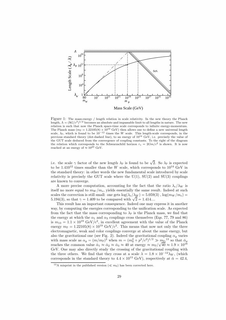
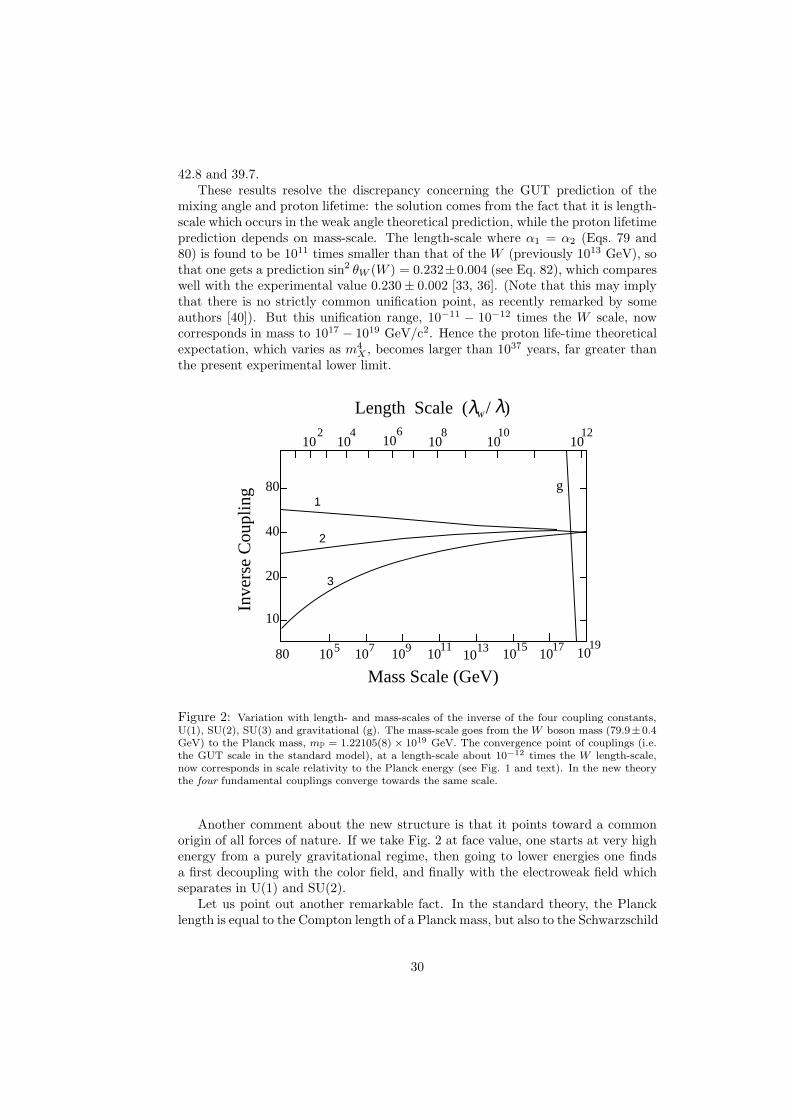


![Hominid evolution: genetics versus memetics. · arXiv:1011.3393v3 [q-bio.PE] 29 Jul 2011 Hominid evolution: genetics versus memetics. Brandon Carter CNRS, LuTh, Observatoire de Paris,](https://static.documents.pub/doc/80x56/5fff19a7f3fda338d44d975c/hominid-evolution-genetics-versus-arxiv10113393v3-q-biope-29-jul-2011-hominid.jpg)

![Simulated [CII] 158 µm observations for SPICA / SAFARI F. Levrier P. Hennebelle, E. Falgarone, M. Gerin (LERMA - ENS) F. Le Petit (LUTH - Observatoire.](https://static.documents.pub/doc/80x56/5a4d1af17f8b9ab05997e928/simulated-cii-158-m-observations-for-spica-safari-f-levrier-p.jpg)


