THE TRANSPORT AND FATE OF CHLORIDE WITHIN THE GROUNDWATER OF

A MIXED URBAN AND AGRICULTURAL WATERSHED

Jessica J. Ludwikowski

56 Pages

Groundwater modeling plays an important role in quantifying solute transport in

watersheds. Many watersheds contain developed or urbanized lands. Urbanized settings

contain impervious surfaces that are highly prone to pollutant run off such as road salt.

Road salt runoff can affect the quality of surface and groundwater resources in addition to

having severe impacts on ecosystems and all ecosystem components. Subsequently,

surface waters and groundwater within Illinois have shown elevated concentrations of

chloride. In a typical winter season in Illinois, about 471,000 tons of road salt are

deposited. About 45% of the deposited road salt will infiltrate through the soils and into

shallow aquifers. A small percentage of chloride remains in the subsurface feeding

shallow aquifers during the non-salting season. Chloride has the potential to reside within

groundwater for years based on the pathway, the geologic material, and the recharge rate

of the aquifer system. However, the relationship between road salt application rates,

residence times, and net mass accumulation of chloride have not been studied.

The transport and fate of chloride in Little Kickapoo Creek watershed (LKCW)

was modeled utilizing MODFLOW, MODPATH, and MT3D. An increase in application

rate showed increases in the mass of chloride within LKCW. Chloride concentrations

reached maximum contaminant level of 250 mg/L after 10 years of deposition exhibiting

how quickly the solute builds up within LKCW. Allowing the solute to return to safe

drinking levels within the watershed took 30 years. Steady-state times varied based on

application rates, lower rates of 1,000 mg/L to 2,500 mg/L took about 60 years, higher

rates never achieved steady-state conditions. Model simulations reveal a positive

relationship between application rate and residence time, the average time a molecule

resides within the reservoir, of chloride. At steady-state conditions, the Cl- residence time

reflects that of groundwater (~1,000 days). Prior to steady-state conditions, residence

time varies from 1,123 to 1,288 days based on application rate.

KEYWORDS: Chloride, Groundwater Modeling, Land use, MODFLOW, MODPATH,

MT3D, Road salt, Watershed, Residence Time

THE TRANSPORT AND FATE OF CHLORIDE WITHIN THE GROUNDWATER OF

A MIXED URBAN AND AGRICULTURAL WATERSHED

JESSICA J. LUDWIKOWSKI

A Thesis Submitted in Partial

Fulfillment of the Requirements

for the Degree of

MASTER OF SCIENCE

Department of Geography-Geology

ILLINOIS STATE UNIVERSITY

2016

© 2016 Jessica J. Ludwikowski

THE TRANSPORT AND FATE OF CHLORIDE WITHIN THE GROUNDWATER OF

A MIXED URBAN AND AGRICULTURAL WATERSHED

JESSICA J. LUDWIKOWSKI

COMMITTEE MEMBERS:

Eric Peterson, Chair

Walt Kelly

David Malone

Catherine O’Reilly

i

ACKNOWLEDGMENTS

I would like to express the deepest appreciation to my committee chair, Professor

Eric Peterson, who has been a supporting and patient advisor through the whole process.

Without his guidance and persistent help this thesis would not have been possible.

I would like to thank my committee members. Professor David Malone, who has

guided me through my graduate academic career and support with the Plate 1. Professor

Catherine O’Reilly for helping me through the graduate program at Illinois State

University. Lastly, Walton Kelly and Daniel Abrams for their very helpful perspective in

groundwater modeling.

Thanks also goes to my fellow graduate students in the Hydrogeology program

with their help providing feedback for the writing process. In addition, I would like to

thank Bill Shields for his technical support in constructing the surficial map.

Finally, I would like to thank my future husband whose encouragement kept me

moving at times when I was beyond overwhelmed. Without his unconditional love and

support I would not have even applied for graduate school nor complete this thesis.

J. J. L.

ii

CONTENTS

Page

ACKNOWLEDGMENTS i

CONTENTS ii

TABLES iv

FIGURES v

CHAPTER

I. INTRODUCTION AND BACKGROUND 1

Introduction 1

Statement of the Problem 2

Sources of Chloride 3

Previous Work 4

Objective 7

Hypotheses 8

II. METHODS AND MATERIALS 9

Watershed Characteristics 9

Conceptual Model 12

Model Setup 13

Sensitivity Analysis 20

III. RESULTS 22

Sensitivity Analysis 22

Flush Scenario Results 25

Build-up Scenario Results 30

MODPATH Results 38

iii

IV. DISCUSSION 41

Residence Time 41

Mass Accumulation – Flush Scenario 42

Mass Accumulation – Build-up Scenario 43

Further Consideration 44

V. CONCLUSION 46

VI. FUTURE CONSIDERATION 48

REFERENCES 49

APPENDIX A: Plate 1 56

iv

TABLES

Table Page

1. Values Used for Model Parameters 17

2. Build-up Scenarios and their Assigned Application Rate 19

v

FIGURES

Figure Page

1. Land Use within the Little Kickapoo Creek Watershed 10

2. Distribution of Geologies Used in Model Simulations 13

3. Boundary Conditions Used in Model 15

4. Sensitivity Analysis MODFLOW Results 23

5. Sensitivity Analysis MT3D Results 24

6. Flush Scenario Results 26

7. Flush Scenario Results 27

8. Flush Scenario Color Flood Map 29

9. Build-up Scenario Results 31

10. Build-up Scenario Results 31

11. Build-up Scenario Results 32

12. Build-up Scenario Results 33

13. Build-up Scenario Results 34

14. Build-up Scenario Results 35

15. Build-up Scenario Results Color Flood Map 36

16. Build-up Scenario Results Color Flood Map 37

vi

17. MODPATH Results 39

18. MODPATH Results 40

1

CHAPTER I

INTRODUCTION AND BACKGROUND

Introduction

The rapid urbanization of the human population in metropolitan areas can have

severe effects on local groundwater resources (Fitzhugh and Richter, 2004; Jenerette and

Laresen, 2006; Oiste, 2014; Villholth, 2006). With urbanization comes impervious

surfaces that are highly prone to run off of pollutants such as road salt (Kelly, 2008).

Road salt is a compound containing chloride (Cl-) and is most commonly found with

cations such as calcium, sodium, or magnesium. Chloride is relatively unreactive on the

Earth’s surface and is considered conservative in nature. Therefore, the properties of Cl-

deem it the perfect tracer of contamination in the environment. The goal of this study is

to model the transport and fate of Cl- in the shallow groundwater of the Little Kickapoo

Creek watershed (LKCW). Numerical simulations can reveal the residence time, the

average time a molecule resides within the reservoir, of Cl- within an aquifer system and

the capacity of an aquifer to store a solute. Upon completion of this model, a better

understanding of contaminant transport in an urbanized watershed will be gained.

2

Statement of the Problem

Road salt runoff can affect the quality of surface and groundwater resources in

addition to having severe impacts on an ecosystem and all its components. The most

obvious effect of Cl- is the degradation of groundwater and surface water quality (Huling

and Hollocher, 1972; Pilon and Howard, 1987; Amrhein et al., 1992; Howard and

Haynes, 1993; Williams et al., 2000; Bester et al., 2006). Organisms that live within

surface waters are impacted by Cl-. Different toxicity thresholds exist among aquatic

organisms, and it is common to see negative effects on aquatic life from levels ranging

from as little as 150 mg/L to as high as 30,330 mg/L depending on the species (Siegel,

2007). Elevated Cl- concentrations have been found to obstruct the reproduction of

aquatic organisms (Beggel and Geist, 2015). The presence of Cl- in lakes is toxic to

plankton, which is a vital food source to fish and amphibians and contributes to the

eutrophication of waters (Evans and Frick, 2001). Of even greater consequence, Cl- in

stream water changes the sign of net nitrogen mineralization from negative, which

consumes inorganic nitrogen, to positive in debris dam material, which results in dams

becoming sources of inorganic nitrogen (Hale and Groffman, 2006). This results in

bacteria becoming unable to help break down nitrogen in the waters making the water

more dangerous and uninhabitable for a variety of aquatic species (Hale and Groffman,

2006). The elevated Cl- concentrations coupled with the presence of acetate, also found in

deicers, can mobilize heavy metals by ion exchange (Granato et al., 1995). Thus, even if

a species is resistant to Cl- the release of heavy metals could be toxic. While Cl- in

3

drinking water is not toxic to humans, water with concentrations exceeding the secondary

drinking water standard of 250 mg/L is classified as non-potable (U.S. EPA, 2011).

Sources of Chloride

Although the focus of this project is contamination via road salt it should be

acknowledged that other sources contribute Cl- to watersheds. There are two categories

from which Cl- can be introduced into the environment: natural sources and

anthropogenic sources (Mullaney et al., 2009). Natural sources consist of oceans,

bedrock, soils, geologic deposits, and volcanic activity (Mullaney et al., 2009).

Anthropogenic sources include landfills, agricultural practices, the chloralkali industry,

septic system discharge, treated wastewater, and road salt (Kelly, 2008; Mullaney et al.,

2009). These anthropogenic sources of Cl- are borne from humans and are primarily

associated with waste disposal. For instance, leachate from landfills is high in Cl- due to

the disposal of cleaning products and food and beverages high in salt and can leak Cl-

into surrounding waters as was witnessed in seven landfills around Illinois resulting in a

median groundwater concentration of 1,284 mg/L. Another anthropogenic source is

human waste associated with septic systems and water treatment plants (Mullaney et al.,

2009). Panno et al reported septic tank effluent can discharge Cl- concentrations as high

as 5,620 mg/L, which could be quite a significant source if the area’s population relies on

this type of disposal (Panno et al., 2005). Other anthropogenic sources of chloride-rich

waste include agriculture production, both row crops production and animal husbandry.

Fertilizers, such as KCl-, deposited on agricultural lands can raise Cl- content in

groundwater and surface waters by as much as 20 mg/L in comparison to the 10 mg/L

4

background levels found in Illinois (Kelly, 2008). Livestock waste, such as animal feed

and urine, contributes Cl- to local waters. Panno et al. (2005) found a median Cl-

concentration of 57 mg/L in groundwater wells near livestock.

In the mid to upper latitudes, the largest contributor of Cl- is road deicers (Kelly,

2008; Mullaney et al., 2009). To maintain safe roadways in the winter, humans have used

salt compounds that decrease the freezing point of water to prevent ice from forming.

These compounds contain Cl-, and when applied to winter roads, a surplus of Cl-

develops. Application rates can vary from 1 to 74 ton(s) per road mile in the Midwest and

eastern states (Jones and Sroka, 1997; Heisig, 2000; Mullaney et al., 2009). In the

northeastern United States, a range of 545 to 23,716 kg/km2/year of road salt is deposited,

much of which will runoff into local surface waters or infiltrate into groundwater (Panno

et al., 2005). Water sources close to roads can contain Cl- concentrations ranging from

2000 mg/L to as high as 14,175 mg/L (Lax and Peterson, 2008; Panno et al., 2005).

Cassanelli and Robbins (2013) report that throughout Connecticut Cl- concentrations in

groundwater have increased by more than an order of magnitude in the last century, an

increase proportionate with Connecticut’s use of road salt.

Previous Work

In groundwater, Cl- is transported differently than in surface waters such as rivers,

streams, lakes, ponds, and wetlands. In rivers and streams, the travel time of Cl- is much

shorter in comparison to groundwater systems. Church and Friesz (1993) concluded that

an estimated 55% of deposited road salt enters local surface water bodies. This results in

a seasonal variance in which spikes of Cl- are observed in surface waters during winter

5

storm events (Williams et al., 2000; Kelly, 2008; Perera et al., 2013; Corsi et al., 2014).

River and stream Cl- loads are detected within hours of road salt deposition unlike the

yearlong increased levels observed in groundwater (Kelly et al., 2012). Chloride can be

retained in surface waters, primarily reservoirs. In the cities of Minneapolis and St. Paul,

a local watershed retained annually 77% of road salt deposited within lakes, wetlands,

ponds, and groundwater (Novotny et al., 2009). However, runoff is not the only pathway

in which Cl- can travel into rivers and streams; it can also be fed from Cl- impacted

groundwater (Cantafio and Ryan, 2014).

In the snow-laden areas of the United States, aquifer systems have been studied

exclusively with respect to Cl-. Since the 1960s, waters within some shallow Chicagoland

aquifers have seen a Cl- increase of 1 mg/L/year or more due to increased road salt

application (Kelly, 2008). This annual increase indicates that Cl- can be stored within

soils and groundwater. While residing within soils, Cl- travels vertically via molecular

diffusion and dispersion feeding groundwater (Lax and Peterson, 2008). Multiple studies

have found that each year a percentage of deposited road salt remains within the

unsaturated zone, supplying Cl- to groundwater through the non-salting season (Mason et

al., 1999; Lax and Peterson, 2008; Kelly et al., 2012; Corsi et al., 2014). As a result, there

is an accumulation of Cl- in groundwater systems. Once in groundwater, Cl- residence

time can be decades to thousands of years, similar to residence times for groundwater,

and therefore, the transport of Cl- will reflect these residence times (Daley et al., 2009).

A host of factors can influence the transport of Cl- through a system. Howard and

Haynes (1993) modeled the inflows and outflows of Cl- in a Toronto watershed utilizing

6

aquifer parameters to find when the watershed would reach steady state. In the model,

parameters such as recharge, aquifer thickness, specific yield, and groundwater flow

velocities played a crucial role in determining when the watershed would reach steady

state with Cl- (Howard and Haynes, 1993). Soil type can also influence the transport of

Cl- (Ramakrishna and Viraraghavan, 2005; Findlay and Kelly, 2011). Finally, hydraulic

conductivity of aquifers, if low, can retard or slow the transport of Cl- within an aquifer

system (Findlay and Kelly, 2011).

Land use in hydrologic systems can similarly affect the transport of Cl-.

Urbanized areas are known to have impervious surfaces that contaminants cannot seep

through. Daley et al. (2009) discovered that areas with high percentages of road

pavement and impervious surfaces have a positive correlation with Cl- concentrations in

surface and groundwater due to runoff from road salt. They conclude that runoff from

impervious surfaces can transport Cl- faster than rural settings (Daley et al., 2009). Lax et

al. (in review) suggest that urban land use as low as 10% results in elevated Cl-

concentrations in stream waters.

Temporal factors can impact the travel of Cl- in hydrologic systems. Obviously,

road salt deposited during winter storm events is one of the leading factors. During

winter-storm season, the frequency and severity of road salt application dramatically

increases temporal Cl- concentrations in streams, lakes, and groundwater (Godwin et al.,

2003; Robinson et al., 2003; Kaushal et al., 2005; Rosfjord et al., 2007; Kelly, 2008;

Daley et al,. 2009). Granato et al. (1995) found in southeastern Massachusetts that winter

recharge rates contributed 75% of the annual subsurface recharge due to low

7

evapotranspiration during winter months. The combination of road salt application and

higher infiltration result in the transport of Cl- into groundwater.

Numerical modeling can quantify the residence time of Cl-, the total solute

storage, and the time when steady state will be reached. Huling and Hollocher (1972)

conducted a study in eastern Massachusetts, which concluded Cl- residence time in

groundwater, at a minimum, exceeded 1 year (Huling and Hollocher, 1972). Boutt et al.

(2001) estimated that transport distances can exceed 10 km in a 50 year period within a

Michigan watershed. This same study also found that the watershed will reach steady-

state conditions in 50 years (Boutt et al., 2001). Howard (1993) completed a mass

balance model that revealed Cl- concentrations in Toronto, Candida would reach steady

state within 60 years of initial salt application. Bester et al. (2006) completed a 3D model

that exhibited Cl- would take decades to flush out of groundwater in an Ontario glacial

moraine aquifer system. Model estimates are site specific but these studies indicate how

Cl- would transport in aquifers of shallow glacial systems. However, none of the models

have compared different application rates and their relationship with Cl- residence time

and mass accumulation.

Objective

The goal of this study is to develop a coupled groundwater-solute transport model

of a shallow aquifer in a central Illinois watershed. Utilizing this model, the relationship

between Cl- and road salt application rates will be investigated. The goal is to examine

the solute residence time and solute storage by simulating different application rates.

Solute storage is the watersheds capacity to accumulate Cl-, which will be referred to as

8

storage from herein. Based on the stability and conservative nature of Cl-, one would

expect that increasing the application rate of road salt will cause Cl- to accumulate within

the aquifer. With Cl- mass accumulating within the watershed the residence time of Cl-

will increase. For this study, residence time is the amount of time the solute, Cl-, travels

from source to sink along a flow path. Thus, if the application rate of road salt increases

then the residence time of Cl-increases. As a result, higher application rates will equate to

a higher total mass of Cl- within the system and longer residence times. In brief, a

positive relationship is posited between road salt application rate and both residence time

and mass of Cl- within an aquifer.

Hypotheses

1. The relationship between the rate of road salt application and the residence time of Cl-

within a shallow aquifer is positive.

2. The relationship between the rate of road salt application and the mass of Cl-

accumulating within a shallow aquifer is positive.

9

CHAPTER II

METHODS AND MATERIALS

Watershed Characteristics

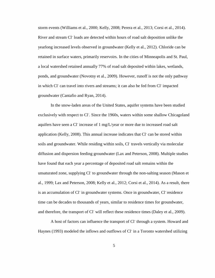
The watershed in this study was located in Bloomington-Normal, McLean

County, Illinois (Figure 1). In 2014, Bloomington’s total population is 78,902 and

Normal has a total population of 54,664; both cities have grown at rates of 3.0% and

4.1% respectively (U.S. Census Bureau, 2014). Little Kickapoo Creek watershed, the

focus of this study, is a part of the greater watershed Kickapoo Creek. The Little

Kickapoo Creek watershed (LKCW) covered a total area of approximately 70 km2, with

the stream running through the center of the watershed and tributaries extending

throughout (Figure 1). Little Kickapoo Creek (LKC) originates in the southeast of

Bloomington, IL and flows to the south-southwest of Bloomington-Normal metropolitan

area. The stream leaves the highly urbanized area and flows through a low-density urban

setting before transitioning into agricultural and forested areas (Figure 1). The land use

was 27% urban, 69% agricultural, and 4% forested/wetland/surface water areas;

classifying the watershed as mixed urban and agricultural (U.S Geological Survey, 2011;

Figure 1).

10

Figure 1: Land Use within the Little Kickapoo Creek Watershed. Data obtained from the

U.S Geological Survey (2011).

A 1:24,000–scale (Plate 1) of the watershed did not exist. To accurately model the

hydrogeology, a surficial geology quadrangle map of the Bloomington-East 7.5 Minute

Quadrangle was completed. The map was constructed using McLean County Soil Survey

11

data, Illinois State Geologic Survey well log data, previous geologic investigations, and

field investigations. Soils data provided information on the parent material of the soil.

ESRI’s ArcGIS 10.2 was utilized for grouping soils based on the parent material. In

addition, ArcGIS 10.2 was used to analyze well logs that provided unit thicknesses; to be

considered mappable, units had to be at least 5 m thick. With geologic units delineated,

the shapefile was imported and redrafted in ACD’s Canvas 11. The completed map was

combined with contour elevations into a GeoPDF, provided by the USGS, using Adobe

Illustrator.

The interpretations of the surficial geology map are consistent to the entirety of

McLean County in which the deposits are glacially borne. The surficial geology is

influenced by the Wisconsin glacial episode wherein two moraines and an outwash plain

are present (Plate 1). The two moraines are the Normal Moraine in the north and the

Bloomington Moraine in the south. Each moraine is comprised of Wedron Group tills;

with the Normal Moraine being of the Lemont Formation and the Bloomington Moraine

consisting of the Tiskilwa Formation (Plate 1). Both tills can be described as red to

grayish-blue diamict clays and gravel, with a hydraulic conductivity (K) of 1.0 x 10-8 m/s

and a thickness of 70 meters (Hensel and Miller, 1991; Plate 1). South of the

Bloomington Moraine is an outwash plain of the Mason Group Henry Formation, which

is a sand and gravel mix with a K of 1.0 x 10-4 m/s and a thickness of 8 to 10 meters

(Ackerman et al., 2015; Plate 1).

12

Conceptual Model

The conceptual model for LKCW was developed using available hydrogeologic

information. Based on the subsurface geologic map, it was decided to construct a one-

layer model that accounts for flow through the glacial sediments. The bedrock underlying

the glacial sediments is mostly low-conductivity Pennsylvanian shale, thus limiting

vertical movement of water in the aquifer. To differentiate between the outwash and till

geologies (Figure 2), the respective cells had assigned hydraulic conductivities to

represent the respective units. Till units identified within Plate 1 were combined into one

major unit. Outwash units are typically thinner than till but it is assumed that the outwash

thickness does not affect transport. The till unit could have been multiple layers due to

the lenses of sand and gravel; it was decided that the lenses extent across the region was

small, and thus, the influence of the lenses on the model was assumed to be negligible. In

this particular region, till units can be as thick as 70 m so cell thickness was set a uniform

100 m among both geologies. The model was classified as 2-D. The till and outwash are

represented as homogeneous and isotropic, but K values differ between the units.

13

Figure 2: Distribution of Geologies Used in Model Simulations.

Model Setup

Boundary conditions were assigned utilizing hydrography data from the National

Hydrography Dataset (U.S. Geological Survey, 2014). The hydrography data included the

boundary of the Kickapoo Creek watershed, parts of which was used to delineate the

14

domain of the LKCW. The domain of the model was limited to the surface water

drainage basin for LKC, assuming that the surface water divide serves as a groundwater

divide for the shallow groundwater system (Figure 3). A no flow boundary existed along

the perimeter and bottom of the domain; recharge was applied across the surface of the

model domain. The surface boundary along the LCK and tributaries was represented with

constant head and solute conditions (Figure 3). Roadways from the National

Transportation Dataset characterized the cells that represent sources of Cl- due to road

salt (Figure 3). Cells that contained roadways had increased Cl- application over the

winter stress period; in the summer the cells returned to background levels. Chloride was

applied to non-urban cells at a constant background rate, 10 mg/L, throughout the entire

simulation. Flow of the system was assumed to be steady-state flow, but the solute

transport (Cl-) was transient due to the seasonal depositional rates.

15

Figure 3: Boundary Conditions Used in Model. The model domain represents the

groundwater divide (black), LKC constant head and constant Cl- concentration (blue),

and roadways constant fluid flux (recharge) and variable rate of for salt application (red).

Groundwater Vistas Version 6 preprocessor allowed the conversion of GIS-based

data to be put into model input files. Incorporating GIS databases into the watershed-

scale model facilitated the ability to apply specific parameters to model cells. The

16

National Hydrologic Dataset provided a shapefile for LKC and the watershed that were

imported in Groundwater Vistas to outline constant head and no-flow boundary cells.

Next, elevation data were applied to the model to depict the top elevation of cells and to

aid the direction of groundwater flow (US Geological Survey, 2013). The National Land

Cover Database assisted in the classification of cells in the model by revealing urban and

agricultural land use locations (Figure 1). Urbanized cells had an increased Cl- value that

reflect those after winter storm events; while agricultural and forested areas had low

constant concentrations through the whole simulation (Figure 1).

Upon completing the application of boundary conditions, parameter values were

added to model cells. Values for each parameter were chosen from previous studies and

literature on the study area (Table 1). Hydrogeologic parameters were applied based on

the geologic unit the cell represented. Other parameters, such as the recharge rate, were

applied uniformly across the watershed despite the varying cell geologies. A recharge

rate of 0.026 cm/day, representing 10% of the annual precipitation, was used along the

top boundary. The recharge value is consistent with other models of the area (Lax and

Peterson, 2008; Van der Hoven et al., 2008). Aquifer test data from wells located in the

modeled area were used to measure storage values for the tills and outwash (Table 1). To

simulate conditions after a winter storm event, urbanized cells (Figure 1) were assigned

elevated Cl- levels of ≥1,000 mg/L provided from shallow monitoring wells installed

along an interstate (Kelly and Roadcap, 1994; Lax and Peterson, 2008; Table 2). The

1,000 mg/L is lower than the measured concentrations within infiltration near a road (Lax

and Peterson, 2008) but given the size of the model cells will be more representative. The

17

non-urban cells had an initial concentration of 10 mg/L simulating background conditions

(Kelly, 2008), and the recharge maintained a constant 10 mg/L concentration over the

duration of the simulation. The model, composed of one layer, simulated transport in the

horizontal dimensions. Model cells are 100 mx100 m, generating a finite-difference grid

with 164 rows, 72 columns, and a total of 7,136 active cells.

Table 1: Values Used for Model Parameters

Stress periods were used to divide the model simulation into seasons. Each year is

broken into two stress periods: 1) winter and 2) summer through fall. The winter stress

period lasted 84 days while the summer through fall spanned the remaining 281 days or

time steps. Following Lax and Peterson (2008), the elevated concentrations of Cl- were

Parameter Value Used Source

Outwash K 1.0 x 10-4

m/s Ackerman et al., 2014

Outwash Porosity 0.35 Ackerman et al., 2014

Outwash Sy 0.021 Field Test (data unreported)

Outwash Ss 0.0007 Field Test (data unreported)

Till K 1.0 x 10-8

m/s Hensel & Miller, 1991

Till Porosity 0.25 Ackerman et al., 2014

Till Ss 0.00056 Field Test

Till Sy 0.01 Field Test

Recharge Rate 2.3 x 102 m/s Lax & Peterson, 2008

Cl- Dispersivity Longitude 1.78 m Giadom et al., 2015

Cl- Dispersivity Latitude 1.64 m Giadom et al., 2015

Cl- Concentration Winter ≥1,000 mg/L Lax & Peterson, 2008

Cl- Concentration Summer 10 mg/L Kelly, 2008

18

applied through the 84 day winter season. As previously stated, the elevated Cl- level was

applied to urban cells, to simulate road salt deposition. Non-urban cells maintained a

constant background level during the entire simulation. Succeeding the winter stress

period, deposition decreased to background levels in the urban cells for the summer

through fall period.

To test the hypotheses, there was seven scenarios. Scenarios 1 and 2 simulated 10

cycles of winter and summer seasons (or 10 years) wherein at the end of year 10, road

salt application ceases and background levels are applied at a constant rate. From years

11 through 60, all cell types have background application. Scenario 1 used Cl- application

rates of 1,000 mg/L whereas Scenario 2 employed 10,000 mg/L. At the end of each

decade, the maximum Cl- concentration and net mass was recorded. Utilizing a basic

mass balance equation the amount of Cl- entering and leaving the system was calculated.

The purpose of the two scenarios was to observe how the watershed flushes out Cl- after

50 years of no deposition and its relationship to the different application rates. Scenarios

3 - 7 simulated a constant, but different, deposition rate across a 60-year span (Table 2).

Varying the application rate provided insight to its relationship with mass build up and

Cl- residence time. For each year, the residence time was calculated using the Equation as

presented by Dingman (2002), where total solute storage and the amount of solute

leaving the system. The maximum concentration and net mass were recorded at the end

of each 5-year period. Herein, Scenarios 1 and 2 are referred to as the “Flush Scenarios”,

while Scenarios 3 – 7 are referred to as the “Build-Up Scenarios”.

19

𝑇𝑟 =𝑇𝑜𝑡𝑎𝑙 𝑀𝑎𝑠𝑠

𝑠𝑜𝑙𝑢𝑡𝑒𝑀𝑎𝑠𝑠 𝑂𝑢𝑡

𝑠𝑜𝑙𝑢𝑡𝑒 Equation 1

Table 2: Build-up Scenarios and their Assigned Application Rate

MODFLOW is a program developed by the United States Geological Survey that

numerically solves the three dimensional groundwater flow equation using the finite

difference method thus simulating groundwater flow (Harbaugh et al., 2000).

MT3D simulates advection, dispersion/diffusion, and chemical reactions of

contaminants in groundwater flow systems using boundary conditions and external

sources or sinks (Zheng and Wang, 1999). To accurately model Cl- movement a

dispersivity coefficient of 1.78 m for longitude and 1.64 m for latitude was employed

(Giadom et al., 2015). Porosity values of the till and outwash units were 0.25 and 0.35

respectively. The solute was distributed via the recharge parameter by assigning a

constant Cl- concentration of ≥1,000 mg/L to cells containing a road or urbanization.

Therefore, the source or Cl-in was recharge and the constant head boundary was the sink

or Cl-out. The constant head boundary was assigned a Cl- concentration of 0 mg/L; no

temporal data existed to apply Cl- that is representative of winter and proceeding seasons.

Scenario Winter Application Rate (mg/L)

3 1,000

4 2,500

5 5,000

6 7,500

7 10,000

20

The concentration remained constant over the 84-day period. Since Cl- is conservative no

retardation factors or reactions were simulated.

MODPATH is a particle tracking post-processing model that computes three-

dimensional flow paths using output from MODFLOW (Pollock, 2012). MODPATH

tracks a particle’s path from cell to cell until it reaches the sink/source or a boundary.

Particles were added to roadways to simulate road salt to observe flow pathways and

particle travel times.

Sensitivity Analysis

Sensitivity analyses were conducted for the groundwater flow model

(MODFLOW) and for the solute transport model (MT3D). Since no data were available

to calibrate the model, the sensitivity analysis was completed to reveal which parameters

the model was sensitive and which had no effect on the model output. The sensitivity

analyses examined how increases and decreases of 25, 50, and 75% for each model

parameter (Table 1) affected the head or concentration within the system. After a percent

change, the model was run and the simulated head or concentration was recorded. In

order to quantify which parameters were sensitive, the observed and simulated values

were compared and the root mean squared error (RMSE) was calculated. Actual observed

values do not exist, therefore values of the base model were used as a comparison

instead. The base model uses an application rate of 1,000 mg/L and the parameter values

listed in Table 1. Base model values were then compared to adjusted simulated values.

Eleven targets were randomly placed within the model domain to track base model and

adjusted values. To choose target locations, the model was broken intro 10 sections. Each

21

section was assigned a set of rows and columns. In Excel, a random number generator

was used to determine the set of rows and columns of each section. If the number pulled

did not lie within the model domain the process was repeated.

22

CHAPTER III

RESULTS

Sensitivity Analysis

With no available field data, the model was not calibrated; instead a sensitivity

analysis was performed. The MODFLOW model was sensitive to recharge, till Kx, and

till Ky (Figure 4). When increasing percent intervals to 75%, the model was most

sensitive to recharge leading to a RMSE of 6.7 m while till Kx was the most sensitive

when decreased 75% with a RMSE of 10.4 m. Although the model was most sensitive to

recharge and till, the initial values of 2.3 x 102 m/s and 1.0 x 10-8 m/s are widely

supported in other studies (Ackerman et al., 2015; Curry, 2007; Lax and Peterson, 2008;

Van der Hoven et al., 2008). Other parameters such as the outwash Kx and Ky did affect

the head of the model but only by 0.3 m after adjusting the parameter by ±75% (Figure

4). The outwash conductivities have a minimal effect on the model head because outwash

cells cover a small area; therefore, outwash conductivities do not have as much of an

influence on the groundwater flow as the till (Figure 4). The MODFLOW model was not

sensitive to changes in porosity, specific yield, or specific storage.

23

Figure 4: Sensitivity Analysis MODFLOW Results. Mean squared error represents head

values (m).

The MT3D model was most sensitive to recharge and till porosity in comparison to

all other parameters (Figure 5). Percent decreases resulted in the model to be most sensitive

to till porosity with an RMSE of 22 mg/L at -75% which represents 11% of the maximum

concentration. Lowering the porosity results in faster groundwater flow and therefore faster

solute transport, which decreases the solute concentration. Increases in the parameters

caused the model to be most sensitive to the recharge volume with an RMSE of 6 mg/L at

75%, which is 3% of the maximum concentration. As per the MODFLOW model, the final

values used for each of these parameters are supported in other studies (Ackerman et al.,

0.00

2.00

4.00

6.00

8.00

10.00

-75 -50 -25 0 25 50 75

RM

SE (

m)

Change from initial value (%)

Outwash Ky Till Kx Outwash Kx Till Ky Recharge

24

2015; Curry, 2007; Lax and Peterson, 2008; Van der Hoven et al., 2008). None of the other

parameters affected the solute transport as much as recharge and till porosity, with the

highest concentration change of 1 mg/L at ±75% (Figure 5). The MT3D model was

insensitive to changes in till and outwash Kx and Ky values. The final values did not change

from those selected as initial parameter values (Table 1).

Figure 5: Sensitivity Analysis MT3D Results. Mean squared error represents Cl-

concentration (mg/L).

0.00

5.00

10.00

15.00

20.00

25.00

-75 -50 -25 0 25 50 75

RM

SE (

mg/

L)

Change from inital value (%)

Till Porosity Outwash Porosity Till SyOutwash Sy Outwash Ss Till SsTill Kx Outwash Kx Recharge

25

Flush Scenario Results

The flush scenarios simulates road salt application of 1,000 or 10,000 mg/L for 10

winter seasons. At year 10, the application of Cl- is shut off, and the model is run for 50

additional years. Upon simulation completion, mass balance data and the maximum Cl-

concentration across the model domain from each decade were recorded. For each

scenario, the maximum Cl- level increases and then peaks right at year 10 for both rates

(Figure 6). After year 10, the levels decrease but never return to initial concentrations as

used in the simulations (Figure 6). For both rates, maximum Cl- levels are a percentage of

the deposition rate even after 10 winter seasons. For instance, when salt was applied at

1,000 mg/L the maximum Cl- level is 85 mg/L or 9% of the rate (Figure 6). The same is

true when applied at 10,000 mg/L, by the end of year 10 the maximum concentration is

767 mg/L or 8% of the application rate (Figure 6). Chloride does not completely return to

background levels of 10 mg/L either. By the end of the simulation, 50 years after

application, the maximum Cl- concentration was 166 and 25 mg/L for 10,000 and 1,000

mg/L rates (Figure 6).

26

Figure 6: Flush Scenario Results. Where road salt was applied for 10 winter seasons and

shut off at end of year 10. Reported is the maximum Cl- concentration (mg/L) at the end

of each decade and the background levels (black).

The flush scenarios mass balance data were used to calculate the net mass of Cl-.

The net mass of Cl- increases and peaks at year 10 for both the 1,000 and 10,000 mg/L

application rates with a mass of 11,800 Kg/L and 127,000 Kg/L respectively (Figure 7).

Thereafter, the mass drops by a little more than half by the simulation end with 6,200

Kg/L for the 1,000 mg/L application rate, which is 53% of mass peak, and 73,500 Kg/L

for the 10,000 mg/L application rate, which is 58% of mass peak (Figure 7).

0

50

100

150

200

250

300

350

400

450

500

550

600

650

700

750

800

0 10 20 30 40 50 60

Max

Cl-

(mg/

L)

Time (years)

Application of 1,000 mg/L Application of 10,000 mg/L Background 10 mg/L

27

Figure 7: Flush Scenario Results. Where road salt was applied for 10 winter seasons and

shut off at end of year 10. Reported is the net mass of Cl- (Kg/L) at the end of each

decade.

A color flood map of both application rates displays the Cl- concentration across

the watershed (Figure 8). In both scenarios, salt builds up within roadways and urbanized

areas (Figure 8). After the application of chloride is ceased, the salt slowly dissipates

from roadways and urbanized areas into surrounding sediments and LKC. This can be

seen by how the Cl- (hotter colors) migrate from deposition areas, especially at year 60

(Figure 8). Still at the end of the 60-year period, Cl- concentrations are highest along

roadways, especially those within areas comprised of till material, and lowest in

agricultural areas (Figure 8). Geologic material influences Cl- removal from the

0.00E+00

2.00E+04

4.00E+04

6.00E+04

8.00E+04

1.00E+05

1.20E+05

1.40E+05

0 10 20 30 40 50 60

Net

Mas

s o

f C

l-(K

g/L)

Time (years)Application of 1,000 mg/L Application of 10,000 mg/L

28

watershed. Cells representing tills have increased Cl- concentrations and continue to store

Cl- despite 50 years of no application (Figure 8 Panel B). The southern tip of the

watershed is comprised mostly of the highly conductive outwash material and therefore,

displays lowest Cl- concentrations despite being near the primary source (Figure 8). The

10,000 mg/L rate has more Cl- in storage than the 1,000 mg/L rate due to Cl- loading in

the low conductivity tills. The decadal color change in the 10,000 mg/L map show the

concentrations and storage depleting through the years (Figure 8).

29

Figure 8: Flush Scenario Color Flood Map. Panel (A) 1,000 mg/L application rate and

panel (B) 10,000 mg/L application rate. Both panels show models in which road salt was

applied for 10 winter seasons; shut off at end of year 10 and then ran at background

levels for 50 years after.

30

Build-up Scenario Results

Build-up scenarios simulate a constant road salt application for 60 winter seasons,

with each scenario having a specific application rate (Table 2). Similar to the flush

scenarios, mass balance data and the maximum Cl- concentrations at five-year intervals

were recorded. As the application rate increases so do the Cl- concentrations within the

system, a linear relationship between the two is implied (Figure 9). For each individual

application rate, the maximum Cl- level increases every year (Figure 10). Application

rates of 7,500 mg/L and 10,000 mg/L show no signs of reaching steady state, but the

lower rates appear to be nearing a plateau by the end of the 60-year simulation (Figure

10). The point at which the watershed reaches steady state is relative to the application

rate; severe application rates such as 10,000 mg/L show the watershed as continually

storing Cl-. Even after a 60-year period, the maximum Cl- levels are only about 19% of

input for all rates. For example, the 10,000 mg/L application rate results in a maximum

Cl- concentration of 1,900 mg/L (Figure 10).

31

Figure 9: Build-up Scenario Results. Relationship between the application rate and the

maximum Cl- concentration at the end of the 60-year simulation.

Figure 10: Build-up Scenario Results. Where road salt was applied for 60 winter seasons.

Reported are the maximum Cl- concentrations (mg/L) at the end of each five-year period.

0

200

400

600

800

1000

1200

1400

1600

1800

2000

- 1,000 2,000 3,000 4,000 5,000 6,000 7,000 8,000 9,000 10,000 11,000

Max

Co

nce

ntr

atio

n (

mg/

L)

Application Rate (mg/L)

0100200300400500600700800900

10001100120013001400150016001700180019002000

0 10 20 30 40 50 60

Max

Cl-

(mg/

L)

Time (years)1,000 mg/L 2,500 mg/L 5,000 mg/L 7,500 mg/L 10,000 mg/L

32

The net mass of Cl- was also computed for build-up models at the end of each

five-year period. Application rate and net mass presents a linear relationship; as the

application rate increases so does the net mass (Figure 11). From the start to year 60, each

simulation shows Cl- mass accumulating annually, with the 1,000 mg/L and 2,500 mg/L

rates exhibiting some plateauing (Figure 12). At the end of year 60, the net mass is

596,000 Kg/L for the 10,000 mg/L application rate and 58,000 Kg/L for the 1,000 mg/L

(Figure 12). As expected, increasing road salt application also increases the net mass of

Cl-.

Figure 11: Build-up Scenario Results. Relationship between the application rate and the

net mass of Cl- at the end of the 60-year simulation.

0.00E+00

1.00E+05

2.00E+05

3.00E+05

4.00E+05

5.00E+05

6.00E+05

7.00E+05

- 1,000 2,000 3,000 4,000 5,000 6,000 7,000 8,000 9,000 10,000 11,000

Net

Mas

s C

l-(K

g/L)

Application Rate (mg/L)

33

Figure 12: Build-up Scenario Results. Where road salt was applied for 60 winter seasons.

Reported are the maximum net mass of Cl-at the end of each five-year period.

The residence time was calculated every year for each application rate using

Equation 1. Application rate and residence time display a positive relationship with a

range of 1,123 to 1,288 days for the rates of 1,000 and 10,000 mg/L (Figure 13). The

residence time of each application rate peaks around year 5 and then levels out thereafter

(Figure 14). In Figure 14, the exponential increase during the years 0 to 5 is due to mass

Cl-out being lower than mass Cl-

in once the peak is reached mass Cl-out begins to equal

mass Cl-in. From years 10 to 60 the residence times start to converge around 1,000 days

reflecting the groundwater residence time (Figure 14).

0.00E+00

1.00E+05

2.00E+05

3.00E+05

4.00E+05

5.00E+05

6.00E+05

7.00E+05

0 5 10 15 20 25 30 35 40 45 50 55 60

Net

Mas

s o

f C

l-(K

g/L)

Time (years)

1,000 mg/L 2,500 mg/L 5,000 mg/L 7,500 mg/L 10,000 mg/L

34

Figure 13: Build-up Scenario Results. Where road salt was applied for 60 winter seasons.

Shown is the maximum solute residence time (days) and application rate (mg/L)

1100

1120

1140

1160

1180

1200

1220

1240

1260

1280

1300

0 1000 2000 3000 4000 5000 6000 7000 8000 9000 10000

Max

imu

m R

esi

de

nce

Tim

e (

day

s)

Application Rate (mg/L)1,000 mg/L 2,500 mg/L 5,000 mg/L 7,500 mg/L 10,000 mg/L

35

Figure 14: Build-up Scenario Results. Where road salt was applied for 60 winter seasons.

Shown is the solute residence time (days) recorded at the end of each simulated year.

Color flood maps of model scenario 2 were constructed to demonstrate the

distribution of Cl- across the watershed. Both map’s roadways and urbanized areas have

the highest concentration of Cl- and the lowest concentrations are found in LKC (Figure

15 and Figure 16). Unlike the first set of color flood maps (Figure 8), the spreading of

higher concentrations surrounding the deposition areas settings exhibit salt overflowing

and storing in the adjacent sediments (Figure 15 and Figure 16). As LKC represents a

point of groundwater discharge, Cl- transport is directed towards LKC. For both

application rates, the agricultural lands have the lowest concentrations due to their

distance from urban areas and roadways (Figure 15 and Figure 16). With both application

0

200

400

600

800

1000

1200

1400

0 10 20 30 40 50 60

Re

sid

en

ce T

ime

(d

ays)

Time (years)1,000 mg/L 2,500 mg/L 5,000 mg/L 7,500 mg/L 10,000 mg/L

36

rates, the Cl- concentration increases over time in the agricultural areas (Figure 15 and

Figure 16). The 10,000 mg/L map uses a different color scale due to reaching

concentrations over 200 mg/L only after 10 years of application (Figure 16).

Figure 15: Build-up Scenario Results Color Flood Map. Chloride concentration color

flood map of model scenario 2 at the 1,000 mg/L application rate. Shown is the model in

which road salt was applied for 60 winter seasons and LKC (white).

37

Figure 16: Build-up Scenario Results Color Flood Map. Chloride concentration color

flood map of model scenario 2 at the 10,000 mg/L application rate. Shown is the model in

which road salt was applied for 60 winter seasons and LKC (blue). White areas indicate

concentrations at or below 200 mg/L.

38

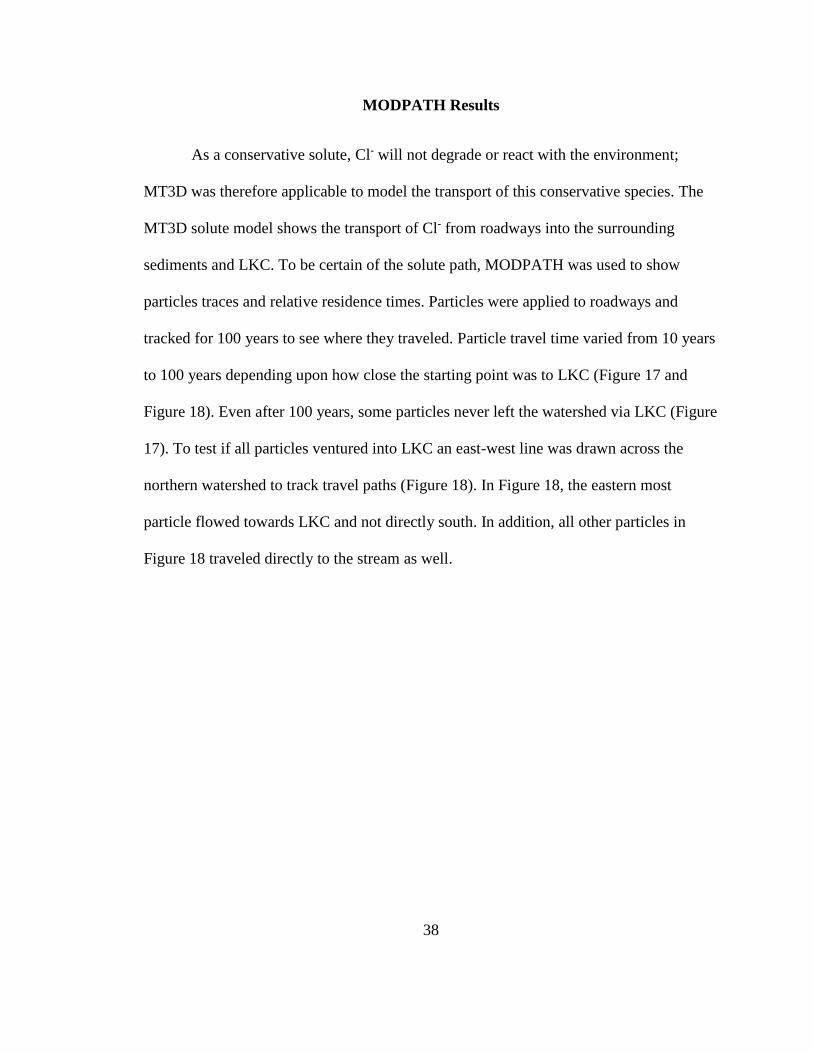
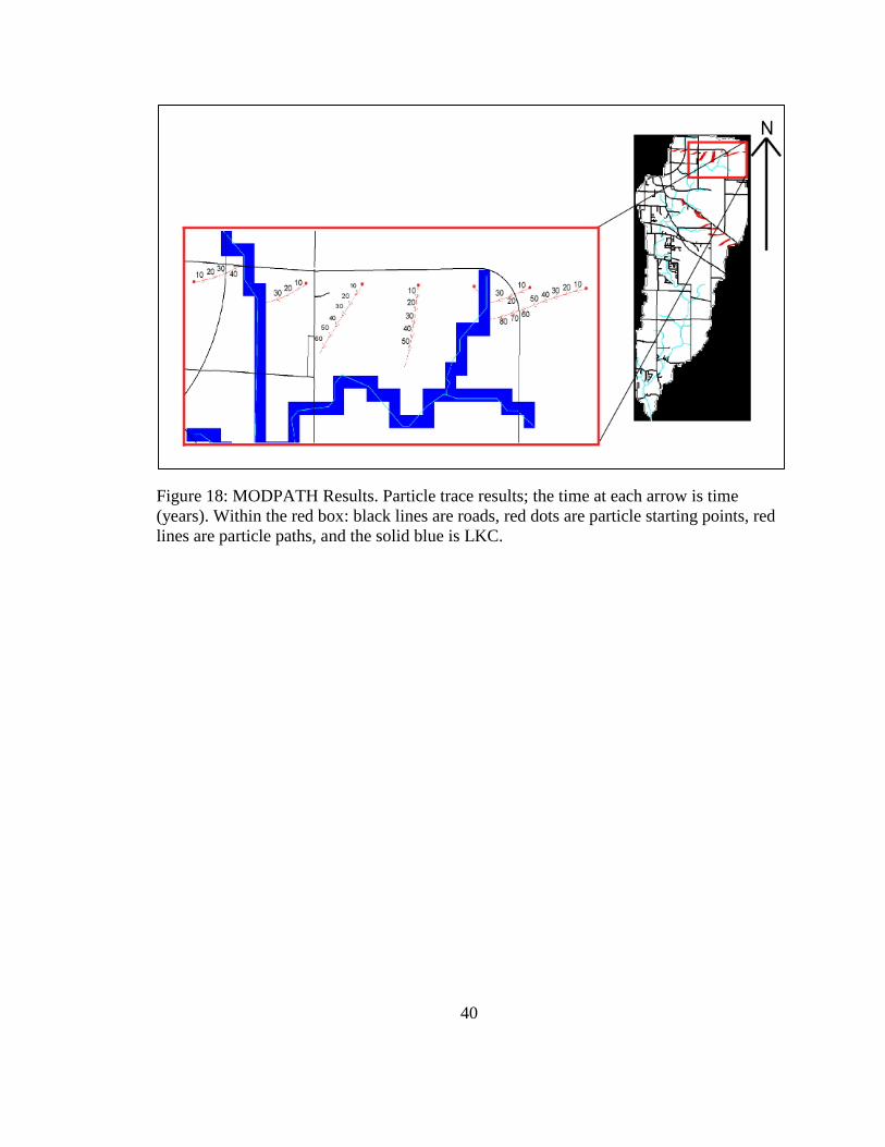
MODPATH Results

As a conservative solute, Cl- will not degrade or react with the environment;

MT3D was therefore applicable to model the transport of this conservative species. The

MT3D solute model shows the transport of Cl- from roadways into the surrounding

sediments and LKC. To be certain of the solute path, MODPATH was used to show

particles traces and relative residence times. Particles were applied to roadways and

tracked for 100 years to see where they traveled. Particle travel time varied from 10 years

to 100 years depending upon how close the starting point was to LKC (Figure 17 and

Figure 18). Even after 100 years, some particles never left the watershed via LKC (Figure

17). To test if all particles ventured into LKC an east-west line was drawn across the

northern watershed to track travel paths (Figure 18). In Figure 18, the eastern most

particle flowed towards LKC and not directly south. In addition, all other particles in

Figure 18 traveled directly to the stream as well.

39

Figure 17: MODPATH Results. Particle trace results; the time at each arrow is time

(years). Within the red box: black lines are roads, red dots are particle starting points, red

lines are particle paths, and the solid blue is LKC.

40

Figure 18: MODPATH Results. Particle trace results; the time at each arrow is time

(years). Within the red box: black lines are roads, red dots are particle starting points, red

lines are particle paths, and the solid blue is LKC.

41

CHAPTER IV

DISCUSSION

Residence Time

The relationship between application rate and Cl- residence time is positive; as the

application rate increases so increases the residence time (Figure 13). This relationship is

especially prevalent in the first 5 years of application where mass is accumulating (Figure

14). At year 5, residence time peaks for all model simulations; thereafter, the residence

time decreases and simulations begin to converge to a value of ~1,000 days (Figure 14).

The decreases observed from years 5 to 60 are due to Cl- mass beginning to reach steady-

state conditions. By year 60, models 3 and 4 are at steady-state conditions (Figure 12),

and the Cl- residence time of ~1,000 days reflects that of the groundwater similar to

Daley et al. (2009) (Figure 14). The Cl- residence time of ~3 years is supported by

MODPATH results (Figure 17 and Figure 18); groundwater residence times of 3 years is

also supported by previous studies (Kelly et al., 2012). Models 5 to 7 are close to steady-

state conditions but have yet to reach the point of diminishing returns (Figure 14). By

graphing the residence time through the entire model simulation we were able to

visualize the ability of the watershed to store and flush Cl- based on each application rate.

Due to Cl- mass still accumulating in higher rates the watershed had yet

42

to reach steady-state conditions thus providing insight into the relationship of application

rate and residence time.

Mass Accumulation – Flush Scenario

Flush models were assigned specific application rates that were applied for 10

winter seasons then shut off. The estimated flush time is relative to application rate with

the application rate of 1,000 mg/L having 47% of its mass flush away while the 10,000

mg/L saw 42% flushed away (Figure 7). The 10,000 mg/L rate took 30 years to return to

the EPA maximum contaminant level of 250 mg/L (Figure 6). Bester et al. (2006)

simulated the transport of a Cl- plume in an industrial/urban aquifer setting; model

simulations indicated Cl- would flush out of the aquifer after four decades of no

application. For both application rates, the simulations show that after 15 years the

maximum Cl- concentrations are half of the peak concentrations, similar to Bester et al

(2006) (Figure 6). Bester et al. (2006) stated that remaining Cl- resided in the low-

conductivity material. The MT3D color flood maps indicate Cl- is stored within the low

conductivity roadside sediments (Figure 8). Solute within the highly conductive outwash

sediments have lower concentrations despite being near the source (Figure 8). This

suggests that the geologic material present influences the flush time, supported by

Howard and Haynes (1993) which suggest that aquifer conductivity influence the

transport of Cl- through a system.

43

Mass Accumulation – Build-up Scenario

Build-up models were assigned application rates that were held constant for 60

years (Table 2). Application rate has a linear relationship with mass accumulation and

groundwater concentration of Cl-, validating the stated hypothesis (Figure 9 and Figure

11). The maximum Cl- concentration within all simulations rose annually at a rate of 1

mg/L (Figure 10), similar to rates reported by Kelly (2008). By year 60, maximum Cl-

concentrations ranged of 197 mg/L to 1,900 mg/L, which are similar to measured Cl-

concentrations in previous studies (Kelly and Roadcap, 1994; Panno et al., 2005; Kelly,

2008; Figure 10). Alarmingly, all models except rates of 1,000 mg/L and 2,500 mg/L

exceeded the MCL after 10 years of deposition (Figure 10). The net mass accumulation is

dependent upon application rate; final net mass ranges from 58 million metric tons to 596

million metric tons, exhibiting a linear relationship with application rates (Figure 12).

Lower rates of 1,000 mg/L and 2,500 mg/L reached steady-state conditions at year 60

contrasting higher rates, suggesting steady-state estimates are dependent on application

rates (Figure 12). For the scenarios examining the lower application rates, estimates of

time to reach steady state matches those of previous studies (Howard and Haynes, 1993;

Boutt et al., 2001). None of those studies took into consideration the relationship

application rates have with accumulation of mass and concentration in the watershed.

This study’s simulations reveal that the watershed exhibits a linear relationship between

with Cl- storage and application rate, which affects steady-state estimates.

44

Further Consideration

At higher rates, 5,000 mg/L to 10,000 mg/L, the simulations exhibit no sign of

reaching steady state after six decades, which is inconsistent with previous estimates

(Howard and Haynes, 1993; Boutt et al., 2001). The estimates differ due to a few reasons.

First, previous studies model transport in different media (i.e. outwash) wherein

groundwater travel times are higher than those of till. As seen in the color flood maps, Cl-

concentrations are highest in tills and lowest in outwash material (Figure 8; Figure 15;

and Figure 16). Other sensitive parameters, such as recharge, can vary depending upon

the region. Unlike the models of Howard and Haynes (1993) and Boutt et al. (2001), the

developed model was not calibrated. While calibration could deem the higher application

rates unrealistic, the recharge rate used in this study was drawn from calibrated flow

models developed for the locale area (Ackerman et al., 2015; Lax and Peterson, 2008).

The application rates greater than 2,500 mg/L would be considered unrealistic when

observing the Cl- concentrations in groundwater wells surrounding a Illinois interstate

(Kelly, 2008; Lax and Peterson, 2008). Land use and the amount of urbanized land within

an area is correlated to higher Cl- levels (Lax et al., in review; Peterson and Benning,

2013). The LKCW could have more urbanized land compared to former models. A

majority of urbanized land occurs in the northern model domain and the headwaters of

LKC, which will extend the amount of time Cl- is in the system. Finally, dissimilar to the

Howard and Hynes (1993) model, the application rate was held constant for the winter

period. Inputting road salt at a constant rate provides only a preliminary estimate of

45

steady-state times. The variation in snowfall would dictate Cl- application rates and affect

the steady-state time.

Color flood maps of the watershed display the distribution of Cl- concentrations

throughout the watershed (Figure 8; Figure 15; and Figure 16). The Cl- concentration is

influenced by the land use of that area. The LKCW is 27% urbanized and 69%

agricultural land uses both of which have associated Cl- concentrations (Figure 1).

Urbanized areas (i.e. roadways) exhibit the highest Cl- concentrations, which is analogous

with (2005) Panno et al. study. Agricultural land use have low Cl- concentrations that

range from 10 mg/L to 50 mg/L which is supported by previous studies (Panno et al.,

2005; Kelly, 2008; Figure 8; Figure 15; and Figure 16). A limitation of the model is the

lack of temporal Cl- concentrations within LKC; the stream was set as a 0 mg/L constant

head boundary, which is why we observe the lowest concentrations along those cells

(Figure 15 and Figure 1). Lax et al. (in review) found that during winter months Cl-

concentrations in an urban stream range between 65 to 1,350 mg/L and for an agricultural

stream between 20 and 60 mg/L. In addition, a seasonal variance in which spikes of Cl-

are observed in surface waters during winter storm events (Williams et al., 2000; Kelly,

2008; Perera et al., 2013; Corsi et al., 2014). Summer Cl- concentrations can also spike

due to contaminated groundwater leaching into LKC (Benning and Peterson, 2012).

Thus, the model lacked simulating LKC seasonal Cl- concentration changes.

46

CHAPTER V

CONCLUSION

Modeling of the watershed revealed 1) the relationship between road salt

application rates and mass solute storage and 2) the relationship between road salt

application rate and solute residence time. A positive relationship was observed between

application rate and mass accumulation. In addition, a positive relationship was observed

between application rate and residence time. The time it takes for the watershed to return

to safe drinking levels is dependent upon the application rate; as the application rate

increases the flush time increases. Steady-state time was also dependent on application

rates, wherein a positive relationship was observed.

The modeling of Cl- transport in this study reveals the proficiency in which a

watershed can store and cleanse road salt. At high application rates, the watershed takes

30 years of no application to return to safe drinking levels, which would not be

achievable due to human dependency on deicers. Lower application rates reached steady-

state conditions after 60 years of deposition. Presently, watersheds within the Midwest

could have reached steady-state conditions with road salt considering application started

in the 1960s. Kelly et al (2012) demonstrated that shallow aquifers within the Chicago

metropolitan area have increased in Cl- concentrations since the 1970s. The Cl-

contaminated groundwater then feeds local streams wherein we observed elevated surface

water Cl- concentrations through non-salting seasons (Kelly et al., 2012). The results of

47

this study display that elevated Cl- concentrations in the groundwater can sustain high

surface water concentrations through the non-salting season. Therefore, with a

continuance of application in the proceeding winter it is possible that surface water Cl-

concentrations will continue to increase through the decades as shown in Kelly et al

(2012) and Kelly et al (2007). Elevated surface waters and groundwater could lead to

detrimental effects on the watershed ecosystem.

48

CHAPTER VI

FUTURE CONSIDERATION

In continuing this studies endeavor, it is necessary to refine the model. A

calibration of the model is essential to ensure accuracy. Layers should be added

effectively simulating the glacial sediments and the geology of the region. The addition

of layers will also introduce surface water-groundwater interactions within the watershed.

Stream data should be pulled from the stream gage station along LKC. Extensive spatial

water sampling of LKC should be conducted over multiple years to model accurately Cl-

levels in the stream. The model should be ran for additional decades to see when

background levels are reached. Lastly, the model should be run until steady state is

reached for all application rates. Many factors can be introduced into the model to help

ensure the validity but nonetheless it must be realized that models are always flawed.

49

REFERENCES

Ackerman, J., Peterson, E., Van der Hoven, S., and Perry, W., 2014, Quantifying nutrient

removal from groundwater seepage out of constructed wetlands receiving treated

wastewater effluent. Department of Geography-Geology, Illinois State University,

(in review).

Amrhein, C., Strong, J., and Mosher, P., 1992, Effect of deicing salts on metal and

organic matter mobilization in roadside soils: Environmental Science Technology,

v. 26, no. 4, p. 703-709, doi:0013-936X/92/0926-0709$03.00/0.

Beggel, S., and Geist, J., 2015, Acute effects of salinity exposure on glochidia viability

and host infection of the freshwater mussel Anodonta anatine: Science of The

Total Environment, v. 502, p. 659-665, doi:10.1016/j.scitotenv.2014.09.067.

Bester, M., Frind, E., Molson, J., and Rudolph, D, 2006, Numerical investigation of road

salt impact on an urban wellfield: Ground Water, v. 44, p. 165-175,

doi:10.1111/j.1745-6584.2005.00126.x.

Church, P., and Friesz P., 1993, Effectiveness of highway drainage systems in preventing

road-salt contamination of groundwater: U.S. Department of the Interior Open-

File Report 96-317, http://pubs.usgs.gov/of/1996/0317/report.pdf (accessed 2013).

Cantafio, L., and Ryan, M., 2014, Quantifying baseflow and water-quality impacts from a

gravel-dominated alluvial aquifer in an urban reach of a large Canadian river:

Hydrogeology Journal, v. 22, no. 4, p. 957-970, doi:10.1007/s10040-013-1088-7.

Corsi, S., De Cicco, L., Lutz, M., and Hirsch, R., 2015, River chloride trends in snow-

affected urban watersheds: increasing concentrations outpace urban growth rate

and are common among all seasons: Science of the Total Environment, v. 508, p.

488-497, doi:10.1016/j.scitotenv.2014.12.012.

Daley, M., Potter, J., and McDowell, W., 2009, Salinization of urbanizing New

Hampshire streams and groundwater, the effects of road salt and hydrologic

variability: Journal of the North American Bethological Society, v. 28, no. 4, p.

929-940, doi: http://dx.doi.org/10.1899/09-052.1.

Dingsman, L.S., 2002, Physical Hydrology: Second Edition, Upper Saddle River, New

Jersey, 24 p.

50

ESRI, 2011, ArcGIS desktop: Release 10.2 Environmental Systems Research Institute:

Redlands, CA.

Evans, M., and Frick, C., 2001, The effects of road salts on aquatic ecosystems.

Environmental Canada, WSTD Contribution No. 02-308:

http://brage.bibsys.no/xmlui/bitstream/id/201102/the_effects_road_salts.pdf

(accessed 2013).

Feth, J., 1981, Chloride in natural continental water a review: U.S. Geological Survey,

Water Supply Paper 2176.

Findlay, S., and Kelly, V., 2011, Emerging indirect and long-term road salt effects on

ecosystems: Year in Ecology and Conservation Biology, v. 1223, p. 58-68, doi:

10.1111/j.1749-6632.2010.05942.x.

Fitzhugh, T., and Richter, B., 2004, Quenching urban thirst, growing cities and their

impacts on freshwater ecosystems: Bioscience, v. 54, p. 741-754,

doi:10.1641/0006-3568(2004)054[0741:qutgca]2.0.co;2.

Gerritse, R., and George, R., 1988, The role of soil organic matter in the geochemical

cycling of chloride and bromide: Journal of Hydrology, v. 101, no. 1–4, p. 83–95,

doi:10.1016/0022-1694(88)90029-7.

Glennon, C., 2008, Evaluating the role of sinuosity in the removal of nitrate from a third

order agricultural stream in central Illinois [Master’s Thesis]: Department of

Geography-Geology, Illinois State University.

Godwin, K., Hafner, S., and Buff, M., 2003, Long-term trends in sodium and chloride in

the Mohawk River, New York, the effect of 50 years of road-salt application:

Environmental Pollution, v. 124, p. 273-281, doi: 10.1016/S0269-7491(02)00481-

5.

Granato G., Church P., and Victoria J., 1995, Mobilization of major and trace

constituents of highway runoff in groundwater potentially caused by deicing

chemical migration: Transportation Research Board.

Hale, R., and Groffman, P., 2006, Chloride effects on nitrogen dynamics in forested and

suburban stream debris dams: Journal of Environmental Quality, v. 35, p. 2425-

2432, doi:10.2134/jeq2006.0164.

Hansel, A., and Johnson, W., 1996, Wedron and Mason Groups, lithostratigraphic

reclassification of deposits of the Wisconsin episode, Lake Michigan lobe area:

Illinois State Geological Survey Bulletin 104.

51

Harbaugh, A., Banta, E., Hill, M., and McDonald, M., 2000, MODFLOW-2000: the U.S.

Geological Survey modular groundwater model: U.S. Geological Survey.

Heisig, P., 2000, Effects of residential and agricultural land use on the chemical quality

of baseflow of small streams in the Croton watershed, southeastern New York:

U.S. Geological Survey, Water Resources Investigations Report 99-4173.

Howard, K., and Haynes, J., 1993, Groundwater contamination due to road deicing

chemicals salt balance implications: Geoscience Canada, v. 20, p. 1-8.

Huling, E.E., and Hollocher, T.C., 1972, Groundwater contamination by road salt:

Steady-state concentrations in east central Massachusetts: Science, v. 176, no.

4032, p. 288–290.

Jenerette, G., and Larsen, L., 2006, A global perspective on changing sustainable urban

water supplies: Global and Planetary Change, v. 50, p. 202-211,

doi:10.1016/j.gloplacha.2006.01.004.

Jones, A., and Sroka, B., 1997, Effects of highway deicing chemicals on shallow

unconsolidated aquifers in Ohio, interim report: 1988-93: U.S. Geological Survey,

Science Investigations Report 2004-5150.

Kaushal, S., Groffman, P., Likens, G., Belt, K., Stack, W., Kelly, V., Band, L., and

Fisher, G., 2005, Increased salinization of fresh water in the northeastern United

States: Proceedings of the National Academy of Sciences of the United States of

America, v. 102, p.13517-13520, doi:10.1073/pnas.0506414102.

Kelly, V., Lovett, G., Weathers, K., Findlay, S., Strayer, D., Burns, D., and Likens, G.,

2008, Long-term sodium chloride retention in a rural watershed, legacy effects of

road salt on stream water concentration: Environmental Science and Technology,

v. 42, p. 410-415, doi:10.1021/es071391l.

Kelly, W., 2008, Long-term trends in chloride concentrations in shallow aquifers near

Chicago: Ground Water, v. 46, p. 772-781, doi:10.1111/j.1745-

6584.2008.00466.x.

Kelly, W., Panno S., and Hackley, K., 2012, Impacts of road salt runoff on water quality

of the Chicago, Illinois, region: Environmental and Engineering Geoscience, v.

18, p. 65-81, doi:10.2113/gseegeosci.18.1.65.

Kelly W., and Roadcap G., 1994, Shallow ground-water chemistry in the Lake Calumet

area, Chicago, Illinois: Proceedings of the National Symposium on Water Quality,

American Water Resources Association, p. 253-262.

52

Keseley, S., 2006, Road salt is a slippery subject: Lake County Health Department and

Community Health Center Cattail Chronicles, v. 16, p. 4–5,

http://www.co.lake.il.us/elibrary/ newsletters/cattail/2007/fall2006.pdf.

Kinoshita, A., Hogue, T., Barco, J., and Wessel, C., 2014, Chemical flushing from an

urban-fringe watershed: hydrologic and riparian soil dynamics: Environmental

Earth Sciences, v. 72, no. 3, p. 879-889, doi:10.1007/s12665-013-3011-x.

Kostick, D., Milanovich, J., and Coleman, R., 2007, 2005 minerals yearbook salt: U.S.

Geological Survey,

http://minerals.usgs.gov/minerals/pubs/commodity/salt/salt_myb05.pdf (accessed

2013).

Lax, S, and Peterson, E., 2008, Characterization of chloride transport in the unsaturated

zone near salted road: Environmental Geology, v. 58, p. 1041-1049,

doi:10.1007/s00254-008-1584-6.

Lax, S., Peterson, E., and Van der Hoven, S., (in review). Quantifying stream chloride

concentrations as a function of land use.

Mason, C., Norton, S., Fernandez, I., and Katz, L., 1999, Deconstruction of the chemical

effects of road salt on stream water chemistry: Journal of Environmental Quality,

v. 28, p. 82-91, doi:10.2134/jeq1999.00472425002800010009x.

Mullaney, J., Lorenz, D., and Arntson, A., 2009, Chloride in groundwater and surface

water in areas underlain by the glacial aquifer system, northern United States:

U.S. Geological Survey, Scientific Investigations Report 2009-5086.

National Oceanic and Atmospheric Administration, 2011, NOAA’s 1981-2010 climatic

normal: U.S. Department of Commerce.

Novotny, E., Sander A., Mohseni O., and Stefan H., 2009, Chloride ion transport and

mass balance in a metropolitan area using road salt: Water Resources, v. 45, p. 1-

13, doi: 10.1029/2009WR008141.

Oiste, A., 2014, Groundwater quality assessment in urban environment: International

Journal of Environmental Science and Technology, v. 11, p. 2095-2102,

doi:10.1007/s13762-013-0477-8.

Panno, S., Hackley, K., Hwang, H., Greenberg, S., Krapac, I., Landsberger, S., and

O'Kelly, D., 2006, Source identification of sodium and chloride in natural waters:

Ground Water v. 44, p. 176-187, doi:10.1111/j.1745-6584.2005.00127.x.

53

Perera, N., Gharabaghi, B., and Howard, K., 2013, Groundwater chloride response in the

Highland Creek watershed due to road salt application: Journal of Hydrology, v.

479, p. 159–168, doi:10.1016/j.jhydrol.2012.11.057.

Peters, N., 1984, Evaluation of environmental factors affecting yields of major dissolved

ions of streams in the United States: U.S. Geological Survey, Water Supply Paper

2228.

Peterson, E., and Sickbert, T., 2006, Stream water bypass through a meander neck,

laterally extending the hyporheic zone: Hydrogeology Journal v. 14, p.1443-1451,

doi:10.1007/s10040-006-0050-3.

Pilon, P., and Howard, K., 1987, Contamination of subsurface waters by road de-icing

chemicals: Water Pollution Research Journal Canada, v. 22, no. 1, p. 157–171.

Pollock, D., 2012, MODPATH: a particle-tracking model for MODFLOW: U.S.

Geological Survey.

Siegel, P., 2007, Hazard identification for human and ecological effect of sodium

chloride road salt: Department of Environmental Services Water Division.

Ramakrishna, D., Viraraghavan, T., 2005, Environmental impact of chemical deicers a

review: Water, Air, and Soil Pollution, v. 166, p. 49-63, doi:10.1007/s11270-005-

8265-9.

Robinson, K., Campbell, J., and Jaworski, N., 2003, Water-quality trends in New

England rivers during the 20th century: U.S. Geological Survey Water-Resources

Investigations Report 03-4012.

Rosfjord, C., Webster, K., Kahl, J., Norton, S., Fernandez, I., and Herlihy, A., 2007,

Anthropogenically driven changes in chloride complicate interpretation of base

cation trends in lakes recovering from acidic deposition: Environmental Science

and Technology, v. 41, p. 7688–7693, doi:10.1021/es062334f.

Rowe, R., and Badv, K., 1996, Chloride migration through clayey silt underlain by fine

sand or silt: Journal of Geotechnical Engineering, v. 122, p. 60-68, doi:0733-

9410/96/0001-0060-0068.

Siegel, P., 2007, Hazard identification for human and ecological effect of sodium

chloride road salt: Department of Environmental Services Water Division.

Sun, H., Alexander, J., Gove, B., Pezzi, E., Chakowski, N., and Husch, J., 2014,

Mineralogical and anthropogenic controls of stream water chemistry in salted

watersheds: Applied Geochemistry, v. 48, p. 141-154,

doi:10.1016/j.apgeochem.2014.06.028.

54

Svensson, T., Lovett, G., and Likens, G., 2012, Is chloride a conservative ion in forest

ecosystems: Biogeochemistry, v. 107, no. 1-3, p. 125-134, doi:10.1007/s10533-

010-9538-y.

U.S. Census Bureau, 2014, State and County Quickfacts:

http://quickfacts.census.gov/qfd/states/17/1706613.html (accessed November

2014)

U.S. Department of the Interior, 2011, Bloomington East Quadrangle, McLean, Illinois,

7.5 Minute Series, Scale 1:24,000.

U.S. Environmental Protection Agency, 2011, 2011 Edition of the Drinking Water

Standards and Health Advisories:

http://water.epa.gov/action/advisories/drinking/upload/dwstandards2011.pdf

(accessed on November 2013).

U.S. Geological Survey, 2013, USGS NED n41w089 1 arc-second 2013 1 x 1 degree

arcgrid: U.S. Geological Survey.

U.S. Geological Survey National Geospatial Technical Operations Center, 2014, National

hydrography dataset best resolution for Illinois 20140729 state or territory

shapefile: U.S. Geological Survey.

U.S. Geological Survey National Land Cover Database, 2011, National land cover

database 2011 impervious surface percentage state extents geotiff: U.S.

Geological Survey.

U.S. Geological Survey National Geospatial Technical Operations Center, 2014, National

transportation dataset for Illinois 20140907 state or territory shapefile: U.S.

Geological Survey.

Van der Hoven, S., Fromm, N., and Peterson, E., 2008, Quantifying nitrogen cycling

beneath a meander of a low gradient, N-impacted, agricultural stream using

tracers and numerical modelling: Hydrological Processes, v. 22, p.1206-1215,

doi:10.1002/hyp.6691.

Villholth, K., 2006, Groundwater assessment and management: implications and

opportunities of globalization: Hydrogeology Journal, v. 14, p. 330-339,

doi:10.1007/s10040-005-0476-z.

Williams, A., Stensland, G., Peters, C., and Osborne, J., 2000, Atmospheric dispersion

study of deicing salt applied to roads, first progress report: Illinois State Water

55

Survey, http://www.isws.illinois.edu/pubdoc/cr/iswscr2000-05.pdf (accessed

2013).

Williams, D., Williams, N., and Cao, Y., 2000, Road salt contamination of groundwater

in a major metropolitan area and development of a biological index to monitor its

impact: Water Resources, v. 34 no. 1, p. 127–138, doi:10.1016/S0043-

1354(99)00129-3.

Zheng, C., and Wang, P., 1999, MT3DMS: A modular three-dimensional multispecies

model for simulation of advection, dispersion and chemical reactions of

contaminants in groundwater systems: U.S. Army Engineer Research and

Development Center

56

APPENDIX A

PLATE 1

See Supplemental File