Theory for the Lasso Recall the linear model Y i = p X j =1 β j X (j ) i + i , i = 1,..., n, or, in matrix notation, Y = Xβ + , To simplify, we assume that the design X is fixed, and that is N (0,σ 2 I )-distributed. We moreover assume that the linear model holds exactly, with some “true parameter value” β 0 . (Part 1) High-dimensional statistics May 2012 1 / 41
Transcript
Theory for the Lasso
Recall the linear model
Yi =
p∑j=1
βjX(j)i + εi , i = 1, . . . ,n,
or, in matrix notation,Y = Xβ + ε,
To simplify, we assume that the design X is fixed, and that ε isN (0, σ2I)-distributed.We moreover assume that the linear model holds exactly, with some“true parameter value” β0.
(Part 1) High-dimensional statistics May 2012 1 / 41
What is an oracle inequality?
Suppose for the moment that p ≤ n and that X has full rank p.Consider the least squares estimator in the linear model
β̂LM := (XT X)−1XT Y.
Then the prediction error
‖X(β̂LM − β0)‖22/σ2
is χ2p-distributed. In particular, this means that
E‖X(β̂LM − β0)‖22n
=σ2
np.
In words: each parameter β0j is estimated with squared accuracy σ2/n,
j = 1, . . . ,p. The overall squared accuracy is then (σ2/n)× p.
(Part 1) High-dimensional statistics May 2012 2 / 41
Sparsity
We now turn to the situation where possi-bly p > n. The philosophy that will gen-erally rescue us, is to “believe” that in factonly a few, say s0, of the β0
j are non-zero.We use the notation
S0 := {j : β0j 6= 0},
so that s0 = |S0|. We call S0 the active set,and s0 the sparsity index of β0.
S0:
(Part 1) High-dimensional statistics May 2012 3 / 41
Notation
βj,S0 := βj l{j ∈ S0}, βj,Sc0
:= βj l{j /∈ S0}.
Clearly,β = βS0 + βSc
0,
andβ0
Sc0
= 0.
(Part 1) High-dimensional statistics May 2012 4 / 41
If we would know S0, we could simply neglect all variables X(j) withj /∈ S0. Then, by the above argument, the overall squared accuracywould be (σ2/n)× s0.
With S0 is unknown, we apply the `1-penalty, i.e., the Lasso
β̂ := arg minβ
{‖Y− Xβ‖22/n + λ‖β‖1
}.
Definition: Sparsity oracle inequality. The sparsity constant φ0 is thelargest value φ0 > 0 such that Lasso β̂ satisfies the φ0-sparsity oracleinequality
‖X(β̂ − β0)‖22/n + λ‖β̂Sc0‖1 ≤
λ2s0
φ20.
(Part 1) High-dimensional statistics May 2012 5 / 41
A digression: the noiseless caseLet X be some measurable space, Q be aprobability measure on X , and ‖ · ‖ be theL2(Q) norm. Consider a fixed dictionary offunctions {ψj}pj=1 ⊂ L2(Q):
Consider linear functions
fβ(·) =
p∑j=1
βjψj(·) : β ∈ Rp.
Consider moreover a fixed target
f 0 :=
p∑j=1
β0j ψj .
We let S0 := {j : β0j 6= 0} be its active set, and s0 := |S0| be the
sparsity index of f 0.(Part 1) High-dimensional statistics May 2012 6 / 41
For some fixed λ > 0, the Lasso for the noiseless problem is
β∗ := arg minβ
{‖fβ − f 0‖2 + λ‖β‖1
},
where ‖ · ‖1 is the `1-norm. We write f ∗ := fβ∗ and let S∗ be the activeset of the Lasso.The Gram matrix is
Σ :=
∫ψTψdQ.
(Part 1) High-dimensional statistics May 2012 7 / 41
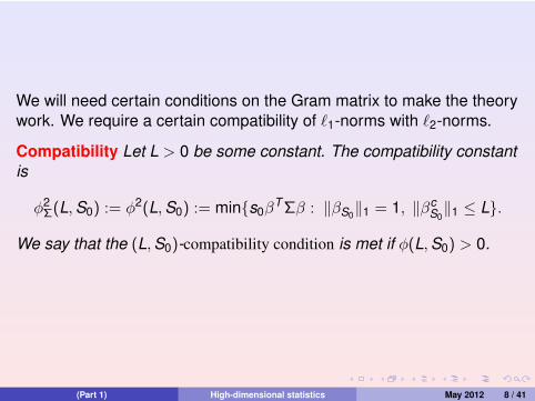
We will need certain conditions on the Gram matrix to make the theorywork. We require a certain compatibility of `1-norms with `2-norms.
Compatibility Let L > 0 be some constant. The compatibility constantis
φ2Σ(L,S0) := φ2(L,S0) := min{s0β
T Σβ : ‖βS0‖1 = 1, ‖βcS0‖1 ≤ L}.
We say that the (L,S0)-compatibility condition is met if φ(L,S0) > 0.
(Part 1) High-dimensional statistics May 2012 8 / 41
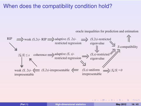
(Part 1) High-dimensional statistics May 2012 14 / 41
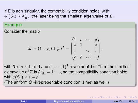
If Σ is non-singular, the compatibility condition holds, withφ2(S0) ≥ Λ2
min, the latter being the smallest eigenvalue of Σ.
ExampleConsider the matrix
Σ := (1− ρ)I + ριιT =
1 ρ · · · ρρ 1 ρ...
. . ....
ρ ρ · · · 1
,
with 0 < ρ < 1, and ι := (1, . . . ,1)T a vector of 1’s. Then the smallesteigenvalue of Σ is Λ2
min = 1− ρ, so the compatibility condition holdswith φ(S0) ≥ 1− ρ.(The uniform S0-irrepresentable condition is met as well.)
(Part 1) High-dimensional statistics May 2012 15 / 41
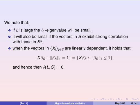
Geometric interpretation
Let Xj ∈ Rn denote the j-th columnof X (j = 1, . . . ,p).The set A := {XβS : ‖βS‖1 = 1}is the convex hull of the vectors{±Xj}j∈S in Rn. Likewise, the setB := {XβSc : ‖βSc‖1 ≤ L} is theconvex hull including interior of thevectors {±LXj}j∈Sc .The `1-eigenvalue δ(L,S) is thedistance between these two sets.
A
B
(L,S)δ
1
(Part 1) High-dimensional statistics May 2012 16 / 41
We note that:
if L is large the `1-eigenvalue will be small,it will also be small if the vectors in S exhibit strong correlationwith those in Sc ,when the vectors in {Xj}j∈S are linearly dependent, it holds that
{XβS : ‖βS‖1 = 1} = {XβS : ‖βS‖1 ≤ 1},
and hence then δ(L,S) = 0.
(Part 1) High-dimensional statistics May 2012 17 / 41
The difference between the compatibility constant and the squared`1-eigenvalue lies only in the normalization by the size |S| of the set S.This normalization is inspired by the orthogonal case, which we detailin the following example.
Example
Suppose that the columns of X are all orthogonal: X Tj Xk = 0 for all
j 6= k . Then δ(L,S) = 1/√|S| and φ(L,S) = 1.
(Part 1) High-dimensional statistics May 2012 18 / 41
Let Sβ := {j : βj 6= 0}. We call |Sβ| the sparsity-index of β. Moregenerally, we call |S| the sparsity index of the set S.
DefinitionFor a set S and constant L > 0, the effective sparsity Γ2(L,S) is theinverse of the squared `1-eigenvalue, that is
Γ2(L,S) =1
δ2(L,S).
(Part 1) High-dimensional statistics May 2012 19 / 41
ExampleAs a simple numerical example, let us suppose n = 2, p = 3, S = {3},and
X =√
n(
5/13 0 112/13 1 0
).
The `1-eigenvalue δ(L,S) is equal to the distance of X3 to line thatconnects LX1 and −LX2, that is
δ(L,S) = max{(5− L)/√
26,0}.
Hence, for example for L = 3 the effective sparsity is Γ2(3,S) = 13/2.Alternatively, when
X =√
n(
12/13 0 15/13 1 0
).
then for example δ(3,S) = 0 and hence Γ2(3,S) =∞. This is due tothe sharper angle between X1 and X3.
(Part 1) High-dimensional statistics May 2012 20 / 41
The compatibility condition is slightly weaker than the restrictedeigenvalue condition of Bickel et al. [2009].The restricted isometry property of Candes [2005] implies therestricted eigenvalue condition.
(Part 1) High-dimensional statistics May 2012 21 / 41
The compatibility condition is slightly weaker than the restrictedeigenvalue condition of Bickel et al. [2009].The restricted isometry property of Candes [2005] implies therestricted eigenvalue condition.
(Part 1) High-dimensional statistics May 2012 21 / 41
Approximating the Gram matrix
For two (positive semi-definite) matrices Σ0 and Σ1, we define thesupremum distance
‖Σ1 − Σ0‖∞ := maxj,k|(Σ1)j,k − (Σ0)j,k |.
Lemma
Assume‖Σ1 − Σ0‖∞ ≤ λ̃.
Then ∀ ‖βSc0‖1 ≤ 3‖βS0‖1,∣∣∣∣∣‖fβ‖2Σ1
‖fβ‖2Σ0
− 1
∣∣∣∣∣ ≤ 16λ̃sφ2
compatible(Σ0,S0).
(Part 1) High-dimensional statistics May 2012 22 / 41
Corollary
We have
φΣ1(3,S0) ≥ φΣ0(3,S0)− 4√‖Σ0 − Σ1‖∞s0.
(Part 1) High-dimensional statistics May 2012 23 / 41
ExampleSuppose we have a Gaussian random matrix
Σ̂ := XT X/n = (σ̂j,k ),
where X = (Xi,j) is a n × p-matrix with i.i.d. N (0,1)-distributed entriesin each column. For all t > 0, and for
λ̃(t) :=
√4t + 8 log p
n+
4t + 8 log pn
,
one has the inequality
P(‖Σ̂− Σ‖∞ ≥ λ̃(t)
)≤ 2 exp[−t ].
(Part 1) High-dimensional statistics May 2012 24 / 41
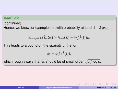
Example(continued)Hence, we know for example that with probability at least 1− 2 exp[−t ],
φcompatible(Σ̂,S0) ≥ Λmin(Σ)− 4√λ̃(t)s0.
This leads to a bound on the sparsity of the form
s0 = o(1/λ̃(t)),
which roughly says that s0 should be of small order√
n/ log p.
(Part 1) High-dimensional statistics May 2012 25 / 41
Definition We call a random variable X sub-Gaussian if for someconstant K and σ2
0,Eexp[X 2/K 2] ≤ σ2
0.
TheoremSuppose X1, . . . ,Xn are uniformly sub-Gaussian with constants K andσ2
0. Then for constants η = η(K , σ20), it holds that
βT Σ̂β ≥ 13βT Σβ − t + log p
n‖β‖21/η2,
with probability at least 1− 2 exp[−t ].
See Raskutti, Wainwright and Yu [2010].
(Part 1) High-dimensional statistics May 2012 26 / 41
General convex lossConsider data {Zi}ni=1, with Zi in some space Z.Consider a linear space F := {fβ(·) =
∑pj=1 βjψj(·) : β ∈ Rp}.
For each f ∈ F , ρf : Z → R be a loss function. We assume that themap f 7→ ρf (z) is convex for all z ∈ Z.For example, Zi = (Xi ,Yi), and ρ is quadratic loss
ρf (·, y) = (y − f (·))2,
or logistic loss
ρf (·, y) = −yf (·) + log(1 + exp[f (·)]),
or minus log-likelihood loss
ρf = f − log∫
exp[f ],
etc.
(Part 1) High-dimensional statistics May 2012 27 / 41
We denote, for a function ρ : Z → R, the empirical average by
Pnρ :=n∑
i=1
ρ(Zi)/n,
and the theoretical mean by
Pρ :=n∑
i=1
Eρ(Zi)/n.
The Lasso isβ̂ = arg min
β
{Pnρfβ + λ‖β‖1
}. (1)
We write f̂ = fβ̂.
(Part 1) High-dimensional statistics May 2012 28 / 41
We furthermore define the target as the minimizer of the theoreticalrisk
f 0 := arg minf∈F
Pρf .
The excess risk isE(f ) := P(ρf − ρf 0).
Note that by definition, E(f ) ≥ 0 for all f ∈ F .We will mainly examine the excess risk E(f̂ ) of the Lasso.
(Part 1) High-dimensional statistics May 2012 29 / 41
Definition We say that themargin condition holds withstrictly convex function G, if
E(f ) ≥ G(‖f − f 0‖).
In typical cases, the mar-gin condition holds withquadratic function G, that is,G(u) = cu2, u ≥ 0, where cis a positive constant. 0.0 0.5 1.0 1.5 2.0
-1.0
-0.5
0.0
0.5
1.0
1.5
2.0
2.5
u
G
-G(u)
uvuv-G(u) H(v)
Definition Let G be a strictly convex function on [0,∞). Its convexconjugate H is defined as
H(v) = supu{uv −G(u)} , v ≥ 0.
(Part 1) High-dimensional statistics May 2012 30 / 41
SetZM := sup
‖β−β0‖1≤M|(Pn − P)(ρfβ − ρfβ0
)|, (2)
and
M0 := H(
4λ√
s0
φ(S0)
)/λ0, (3)
where φ(S0) = φcompatible(S0).Set
T := {ZM0 ≤ λ0M0}. (4)
(Part 1) High-dimensional statistics May 2012 31 / 41
Theorem
(Oracle inequality for the Lasso)Assume the compatibility condition and the margin condition withstrictly convex function G. Take λ ≥ 8λ0. Then on the set T given in(4), we have
E(f̂ ) + λ‖β̂ − β0‖1 ≤ 4H(
4λ√
s0
φ(S0)
).
(Part 1) High-dimensional statistics May 2012 32 / 41
Corollary
Assume quadratic margin behavior, i.e., G(u) = u2. ThenH(v) = v2/4, and we obtain on T ,
E(f̂ ) + λ‖β̂ − β0‖1 ≤4λ2s0
φ2(S0).
(Part 1) High-dimensional statistics May 2012 33 / 41
`2-rates
To derive rates for ‖β̂ − β0‖2, we need a stronger compatibilitycondition.
DefinitionWe say that the (S0,2s0)-restricted eigenvalue condition is satisfied, withconstant φ = φ(S0,2s0) > 0, if for all N ⊃ S0, |N | = 2s0, and allβ ∈ Rp, that satisfy ‖βSc
0‖1 ≤ 3‖βS0‖1, and |βj | ≤ ‖βN\S0‖∞, ∀ j /∈ N , it
holds that‖βN ‖2 ≤ ‖fβ‖/φ.
(Part 1) High-dimensional statistics May 2012 34 / 41
Lemma
Suppose the conditions of the previous theorem are met, but now withthe stronger (S0,2s0)-restricted eigenvalue condition. On T ,
‖β̂ − β0‖22 ≤ 16(
H(
4λ√
s0
φ
))2
/(λ2s0) +λ2s0
4φ4 .
In the case of quadratic margin behavior, with G(u) = u2, we then geton T ,
‖β̂ − β0‖22 ≤16λ2s0
φ4 .
(Part 1) High-dimensional statistics May 2012 35 / 41
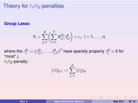
Theory for `1/`2-penalties
Group Lasso
Yi =
p∑j=1
( T∑t=1
X (j)i,t β
0j,t
)+ εi , i = 1, . . . ,n,
where the β0j := (β0
j,1, . . . , β0j,T )T have sparsity property β0
j ≡ 0 for“most” j .`1/`2-penalty:
‖β‖2,1 :=
p∑j=1
‖βj‖2.
(Part 1) High-dimensional statistics May 2012 36 / 41
Multivariate linear model
Yi,t =
p∑j=1
X (j)i,t β
0j,t + εi,t , , i = 1, . . . ,n, t = 1, . . . ,T ,
with for β0j := (β0
j,1, . . . , β0j,T )T , the sparsity property β0
j ≡ 0 for “most” j .Linear model with time-varying coefficients
Yi(t) =
p∑j=1
X (j)i (t)β0
j (t) + εi(t), i = 1, . . . ,n, t = 1, . . . ,T ,
where the coefficients β0j (·) are “smooth” functions, with the sparsity
property that “most” of the β0j ≡ 0.
(Part 1) High-dimensional statistics May 2012 37 / 41
High-dimensional additive model
Yi =
p∑j=1
f 0j (X (j)
i ) + εi , i = 1, . . . ,n,
where the f 0j (X (j)
i ) are (non-parametric) “smooth” functions, withsparsity property f 0
j ≡ 0 for “most” j .
(Part 1) High-dimensional statistics May 2012 38 / 41
Theorem
Consider the group Lasso
β̂ = arg minβ
{‖Y− Xβ‖22/n + λ
√T‖β‖2,1
},
where λ ≥ 4λ0, with
λ0 =2√n
√1 +
√4x + 4 log p
T+
4x + 4 log pT
.
Then with probability at least 1− exp[−x ], we have
‖Xβ̂ − f0‖22/n + λ√
T‖β̂ − β0‖2,1 ≤24λ2TS0s0
φ20
.
(Part 1) High-dimensional statistics May 2012 39 / 41
Theorem
Consider the smoothed group Lasso
β̂ := arg minβ
{‖Y− Xβ‖22/n + λ‖β‖2,1 + λ2‖Bβ‖2,1
},
where λ ≥ 4λ0. Then on
T := {2|εT Xβ|/n ≤ λ0‖β‖2,1 + λ20‖Bβ‖2,1},
we have
‖f̂ − f 0‖2n + λpen(β̂ − β0)/2 ≤ 3{
16λ2s0/φ20 + 2λ2‖Bβ0‖2,1
}.
(Part 1) High-dimensional statistics May 2012 40 / 41
etc. . . .
(Part 1) High-dimensional statistics May 2012 41 / 41