Journal of Magnetism and Magnetic Materials 541 (2022) 168528
A0(
Contents lists available at ScienceDirect
Journal of Magnetism and Magnetic Materials
journal homepage: www.elsevier.com/locate/jmmm
Theory of superlocalized magnetic nanoparticle hyperthermia: Rotatingversus oscillating fieldsZs. Iszály a, I.G. Márián a,b, I.A. Szabó a, A. Trombettoni c,d,e, I. Nándori a,b,f,∗
a University of Debrecen, H-4010 Debrecen P.O. Box 105, Hungaryb MTA-DE Particle Physics Research Group, P.O. Box 51, H-4001 Debrecen, Hungaryc Department of Physics, University of Trieste, Strada Costiera 11, I-34151 Trieste, Italyd CNR-IOM DEMOCRITOS Simulation Center, Via Bonomea 265, I-34136 Trieste, Italye SISSA, Sezione di Trieste, Via Bonomea 265, I-34136 Trieste, Italyf MTA Atomki, P.O. Box 51, H-4001 Debrecen, Hungary
The main idea of magnetic hyperthermia is to increase locally the temperature of the human body by meansof injected superparamagnetic nanoparticles. They absorb energy from a time-dependent external magneticfield and transfer it into their environment. In the so-called superlocalization, the combination of an appliedoscillating and a static magnetic field gradient provides even more focused heating since for large enoughstatic field the dissipation is considerably reduced. Similar effect was found in the deterministic study of therotating field combined with a static field gradient. Here we study theoretically the influence of thermal effectson superlocalization and on heating efficiency. We demonstrate that when time-dependent steady state motionsof the magnetization vector are present in the zero temperature limit, then deterministic and stochastic resultsare very similar to each other. We also show that when steady state motions are absent, the superlocalizationis severely reduced by thermal effects. Our most important finding is that in the low frequency range (𝜔 → 0)suitable for hyperthermia, the oscillating applied field is shown to result in two times larger intrinsic losspower and specific absorption rate then the rotating one with identical superlocalization ability which hasimportance in technical realization.
1. Introduction
Magnetic nanoparticle hyperthermia [1–7], or magnetic fluid hyper-thermia, is an adjuvant cancer therapy where magnetic nanoparticlesare injected into the body. The nanoparticles are used to transfer energyfrom the applied (usually alternating) magnetic field in order to locallyincrease the temperature, which is used to treat cancer. The idea touse temperature increase of the human body for medical applicationshas an ancient history. However, the whole-body hyperthermia haslimitations since it is very difficult to increase the core temperatureof the human body and if we do so it could have serious drawbacks.Thus, one should turn to local heating. The more local the hyperther-mia the more effective the treatment is. In general targeted magnetichyperthermia has a great importance [8,9]. Magnetic nanoparticles canbe used to achieve a very focused, very well localized heating of thehuman body. Indeed, there is an increasing interest on how to improvethe efficiency of the heat transfer, see e.g., [10–12], and also on howto keep the injected particles localized, since they can accumulatein non-targeted tissues [13]. A spatially controlled and image guided
∗ Corresponding author at: University of Debrecen, H-4010 Debrecen P.O. Box 105, Hungary.E-mail address: [email protected] (I. Nándori).
nanoscale magnetic hyperthermia have been recently tested in vivo andin vitro experiments [14]. This method is based on a combination ofan applied alternating and a static field gradient which provides aspatially focused heating [15–19]. The reason is that for large enoughstatic field the dissipation drops to zero, and therefore the temperatureincrease is observed mostly where the static field vanishes. This is aninstance of the phenomenon referred to as ‘‘superlocalization’’, i.e., thecontrollable localization of the temperature increase by the usage ofcombinations of inhomogeneous static and time-dependent magneticfields. This can also be understood by considering the area of thedynamic hysteresis loops. For oscillating applied field, the area of thedynamic hysteresis loops becomes narrow if the static field is present,thus, the amount of energy transferred is decreased and one expectsa bell-shaped curve of the energy transfer as a function of the staticfield amplitude, see, e.g., Fig. (10.4) of [12] or for more details [20].The idea of spatially focused, i.e., superlocalized selective heating of adesired region provides us a very precise heating mechanism which isrealized in recent in vivo experiments [14].
Journal of Magnetism and Magnetic Materials 541 (2022) 168528Z. Iszály et al.
fi
dT
wvn
dTwtc
b
f
oofm1a
A recent proposal [21] discusses the possibility of a superlocalizedand enhanced magnetic hyperthermia by an appropriately chosen com-bination of static and rotating applied fields where the amplitudes ofthe (in-plane) static and rotating fields fulfill a certain relation. For ex-ample, in case of magnetically isotropic nanoparticles the amplitudes ofthe applied magnetic field (static and rotating) should be the same. Theadvantage of the method presented in [21] is the drastic enhancementof the heat transfer which can be very well localized by a static fieldgradient, i.e., spatially controlled by the ratio of the amplitudes of thestatic and rotating applied fields. Another recent example is Ref. [22],where the dynamics and the energy dissipation in the presence of astatic and rotating fields have been studied and enhancement effectsare reported, however the frequency range is too large to be applicablefor hyperthermia. Indeed, the applied external magnetic field is one ofthe most easily variable parameters to increase the efficiency of heatgeneration and one finds several attempts in the literature where thecase of the rotating external magnetic field has been studied, as anexample see the selection [23–36].
If the applied frequency is high enough (𝜔 ≳ 100 kHz) and thediameter of the nanoparticle is appropriately chosen (typically smallenough), the mechanical rotation of the nanoparticles in the surround-ing medium is restricted and one can estimate the efficiency of the heattransfer by considering the change in the orientation of the magnetiza-tion vector, which is called the Neel relaxation process, [35–38]. Onthe other hand the applied frequency and the product of the frequencyand field amplitude cannot be arbitrarily large due to the biologicallimitation of hyperthermic treatment of the human body [38–40]. Onthe one hand, in order to minimize eddy currents, the limiting thresholdfor frequencies is beyond several hundred kHz (certainly not morethan 1000 kHz). On the other hand, the product (of the frequencyand field strength) is related to the power injected, so, it has to besmaller then an upper bound, the so called Hergt–Dutz limit [38–40].General advice is to use a field frequency of several hundred kHz incombination with rather low field amplitude (few kA/m) or a relativelyhigh field amplitude (a few tens of kA/m) in combination with afrequency of a few hundred kHz. Therefore, if the applied frequencyand the applied field amplitude are chosen appropriately, it can beused for hyperthermia and in addition the energy loss depends on thedynamics of the magnetization only, which can be described by the socalled Landau–Lifshitz–Gilbert (LLG) equation [41,42]. Let us note thata different theoretical approach to study the relaxation and obtain thedynamic hysteresis loop is the use of the so called Martensyuk, Raikher,and Shliomis (MRSh) equation, which has been applied to considerthe focused (superlocalized) hyperthermia in [20]. The MRSh equationstands for the average magnetization but the LLG equation describesthe dynamics of a single magnetic moment which is used to calculatethe time-dependence of the average moment. In this work we rely onthe LLG approach.
In view of experimental realizations, it is crucial to consider theinfluence of thermal fluctuations. Such effects were not taken intoaccount in study of the dynamics of the magnetization performedusing the deterministic LLG equation, such as in [21]. The effectof thermal fluctuations can be studied by using the stochastic LLGapproach [43,44]. The motivation of the present work is to explorehow thermal fluctuations can affect the superlocalization in presenceof static and alternating (oscillating or rotating) fields. Thus, our maingoal here is to investigate the influence of thermal effects by means ofthe stochastic LLG equation on superlocalization and heating efficiency,and to compare the rotating and oscillating cases in the presence of astatic magnetic field.
Although, we show that the combination of static and rotatingfields can have importance in the technical realization of magneticnanoparticle hyperthermia, we put serious limitations on the heatingefficiency of the rotating applied field compared to the usual oscillating
2
one.
2. Deterministic and stochastic LLG equations
In the following, we use various types of approximations whichsimplifies the treatment and allow for to get qualitative results onthe dependence of the heat transfer on the parameters of the mag-netic fields. First, we shall consider individual nanoparticles with asingle magnetic domain, so we do not take into account the possibleaggregation of these isolated particles, which usually decreases theefficiency of the heat transfer. As mentioned above, only the changeof the orientation of the magnetic moments are considered and weneglect the effects coming from the rotation of the particle as a wholewhich is a suitable approximation if the applied frequency is high andthe diameter of the particles is small enough. We do not study thedependence of our results on the size of the nanoparticles. Therefore,we use a typical choice for their diameter which is ∼ 20 nm, see belowor more comments on this point. Finally, we assume magneticallysotropic nanoparticles.
As discussed in the introduction, we use here the LLG equation toetermine the motion of the magnetic moment of a single nanoparticle.he Gilbert-form of the deterministic LLG equation readsdd𝑡𝐌 = −𝜇0𝛾0𝐌 ×
[
𝐇eff − 𝜂 dd𝑡𝐌]
, (1)
ith the unit vector 𝐌 = 𝐦∕𝑚𝑆 , where m stands for the magnetizationector of a single-domain particle normalized by the saturation mag-etic moment 𝑚𝑆 (e.g., 𝑚𝑆 ≈ 105 A/m for a single crystal Fe3O4 [45]).
Moreover, 𝛾0 = 1.76 × 10¹¹ A m2/Js is the gyromagnetic ratio, 𝜇0 =4𝜋 × 10−7 Tm/A (or N/A2) is the permeability of free space, 𝜂 is theamping factor and finally 𝐇eff is the local effective magnetic field.he LLG equation retains the magnitude of the magnetization (this ishy one can introduce a unit vector for the magnetization) and only
he orientation changes in time. It is therefore convenient to use polaroordinates [46].
Following the notation of Refs. [21,47–49], the Gilbert-form (1) cane equivalently rewritten asdd𝑡𝐌 = −𝛾 ′[𝐌 ×𝐇eff ] + 𝛼′[[𝐌 ×𝐇eff ] ×𝐌], (2)
which is the LLG equation where 𝛾 ′ = 𝜇0𝛾0∕(1 + 𝛼2), 𝛼′ = 𝛾 ′𝛼 withthe dimensionless damping 𝛼 = 𝜇0𝛾0𝜂. Typical values for the dampingparameter 𝛼 are 𝛼 = 0.1 and 𝛼 = 0.3, which have been used in [32]and [50], respectively. In this paper we use 𝛼 = 0.05, 𝛼 = 0.1 and𝛼 = 0.3.
The local effective magnetic field contains the external applied andthe anisotropy fields. As mentioned above, we consider only sphericallysymmetric nanoparticles without any crystal field anisotropy so, thenanoparticles are considered as isotropic. Several different type ofexternal applied fields combination of static and alternating terms canbe considered. The latter can be either oscillating or rotating:
Rotating ∶ 𝐇eff = 𝐻(
cos(𝜔𝑡) + 𝑏0, sin(𝜔𝑡), 0)
, (3)
Parallel oscillating: 𝐇eff = 𝐻(
cos(𝜔𝑡) + 𝑏0, 0, 0)
, (4)
Perpendicular oscillating: 𝐇eff = 𝐻(
cos(𝜔𝑡), 𝑏0, 0)
, (5)
where 𝐻 and 𝐻𝑏0 stands for the amplitude of the applied and the staticields, respectively.
The heat transfer is a monotonic increasing function of the productf the applied frequency and the field amplitude but at the same timene cannot increase them too much, otherwise they would not usableor medical applications [38–40]. For example, the heating efficiency ofagnetic nanoparticles was considered for relatively high amplitudes00 kA/m at 150 kHz in [51]. The upper bound on the product ofmplitude and frequency is the Hergt–Dutz limit and the value 5 × 10⁸
A/(m s) is used as a safe operational guideline [12]. In other experi-mental studies it was found that this upper limit might be exceeded by
a factor of 10. Indeed, an example for clinical application, one should
Journal of Magnetism and Magnetic Materials 541 (2022) 168528Z. Iszály et al.
etalsdimbtc
𝛼
Tc𝛼
𝛼
wpf
𝛼
𝛼
𝛼
Fct
wr
mention the human-sized magnetic field applicator (developed by Mag-Force Nanotechnologies AG Berlin, Germany) which can generate a 100kHz alternating magnetic field at a variable field strength of 0 − 18kA/m, [52,53] which results in 2 × 10⁹ A/(m s) as an upper limit. Toxplore the dependence on other parameters it is therefore reasonableo keep the product of the frequency and the field amplitude as larges possible. Thus, in this work our choice for the upper (theoretical)imit is 𝜔 ≈ 1000 kHz and 𝐻 ≈ 18kA/m although it is above theafe operational limit. Of course, the Hergt–Dutz limit allow us to useifferent values for 𝜔 and 𝐻 but always keeping their product belowts maximum value and in addition keeping the frequency below itsaximum which is 𝜔 ≈ 1000 kHz. In this work we fix 𝐻 = 18 kA/m
ut in the very last section where we perform a systematic search forhe optimal choice for 𝜔 and 𝐻 both for the oscillating and the rotatingases. We define as well the parameters
𝜔𝐿 = 𝐻𝛾 ′
𝑁 = 𝐻𝛼′. (6)
hus, if one takes 𝛼 = 0.1 (and 𝐻 = 18 kA/m), a good and typicalhoice for parameters suitable for hyperthermia is 𝜔𝐿 = 4 × 10⁹ Hz and𝑁 = 4 × 10⁸ Hz. One can introduce the dimensionless parameters
𝜔 → 𝜔𝑡0𝜔𝐿 = 𝐻𝛾 ′ → 𝜔𝐿𝑡0
𝑁 = 𝐻𝛼′ → 𝛼𝑁 𝑡0. (7)
here the dimension has been rescaled by a suitably chosen timearameter 𝑡0. Here we use 𝑡0 = 0.5 × 10⁻¹⁰ s. In summary, we use theollowing sets of dimensionless parameters:
= 0.05 ⇒ 𝜔𝐿 ∼ 0.2, 𝛼𝑁 ∼ 0.01,
= 0.1 ⇒ 𝜔𝐿 ∼ 0.2, 𝛼𝑁 ∼ 0.02,
= 0.3 ⇒ 𝜔𝐿 ∼ 0.2, 𝛼𝑁 ∼ 0.06. (8)
or hyperthermia one has to take the low-frequency limit, so, a realistichoice for the dimensionless frequency is 𝜔 ∼ 10−4 which correspondso the dimensionful value ∼ 2 × 10⁶ Hz.
As a next step we introduce the stochastic LLG equation [43,44]here thermal fluctuations are taken into account by introducing a
andom magnetic field, 𝐇, in Eq. (1):dd𝑡𝐌 = −𝜇0𝛾0𝐌 ×
[
(𝐇eff +𝐇) − 𝜂 dd𝑡𝐌]
. (9)
The corresponding stochastic form of the deterministic LLG equation(2) can be written asdd𝑡𝐌 = −𝛾 ′[𝐌 × (𝐇eff +𝐇)] + 𝛼′[[𝐌 × (𝐇eff +𝐇)] ×𝐌], (10)
where the stochastic field, 𝐇 = (𝐻𝑥,𝐻𝑦,𝐻𝑧), consists of Cartesiancomponents which are independent Gaussian white noise variableswith the following properties,
where 𝑖 = 𝑥, 𝑦, 𝑧 and 𝐷 is a parameter defined using the fluctuation–dissipation theorem as 𝐷 = 𝜂𝑘𝐵𝑇 ∕(𝑚𝑠𝑉 𝜇0) with the Boltzmann factor𝑘𝐵 , absolute temperature 𝑇 and the volume of the particle 𝑉 , seee.g., [54]. Let us draw the attention of the reader to the dependenceof the stochastic description on the volume of the particles. We do notinvestigate in particular the dependence of our results on the diameterof the individual particles, but the volume cannot be too small sincethen the nanoparticles will not stored in the human body a long enoughtime and, at the same time it cannot be too large because then particleshave multiple magnetic domains which is not favorable regarding theheating efficiency. A typical choice for the diameter is around 20−50 nmand we adopt the size 20 nm in this work.
In Eq. (11) the angular brackets stand for averaging over all possiblerealizations of the stochastic field 𝐇(𝑡). Due to the Gaussian white noise
3
nature of the stochastic field, the random process of 𝐌(𝑡) is a Markovianone. So, one can use the Fokker–Planck formalism. We observe thatit is known that in the semi-classical limit the Keldysh functionalapproach reduces to the Fokker–Planck equation. The general pathintegral approach in the framework of effective field theories usingrenormalization group techniques is still an active research field, seee.g., [55,56].
The stochastic LLG equation (10) can be reduced to (or equivalentlyrewritten as) a system of two stochastic differential equations for thepolar 𝜃 and azimuthal 𝜙 angles, see Refs. [29,30,50]. In a sphericalcoordinate system the effect of the thermal bath appears as a Brownianmotion on a sphere, which can be described by the Ito process
dd𝑡𝜙 = 1
sin 𝜃
√
12𝜏𝑁
𝑛𝜙, (12)
dd𝑡𝜃 = 1
2𝜏𝑁cos 𝜃sin 𝜃
+
√
12𝜏𝑁
𝑛𝜃 . (13)
Here 𝜏𝑁 ∝ 1∕𝑇 is the Néel time for which we used the value 𝜏𝑁 =1.5×10⁻⁷ s at 𝑇 = 300 K. The role of the random white noise is played bythe Gaussian variables 𝑛𝜙 and 𝑛𝜃 , which satisfy the standard properties
Of course these equations are only valid without external fields, how-ever the rhs. of Eqs. (12) (13) represents the only difference betweenthe stochastic and deterministic LLG equation. In 𝑇 → 0 these termsvanish and the stochastic LLG equation reduces to the deterministicone. We developed codes to solve numerically the stochastic differ-ential equations in the presence of a static and rotating applied fielddefined by Eqs. (3), (4) and (5). The codes are written in pythonand Mathematica [57] where the built-in functions for Ito processesare used. Consistency checks and a specific example are shown inAppendix A. In the more complicated cases below, the procedure isthe same, the stochastic LLG equations are solved in the same mannerin the spherical coordinate system, however the equations are lengthywithout containing meaningful new information and thus they are notwritten.
The energy loss in a single cycle can be easily obtained if thesolution 𝐌 of the LLG equation is known:
𝐸 = 𝜇0𝑚𝑆 ∫
2𝜋𝜔
0d𝑡(
𝐇eff ⋅𝑑𝐌𝑑𝑡
)
. (15)
Two important notes are in order, (i) the above formula containsthe average magnetization 𝐌, (ii) it holds for a single particle moreprecisely it has a dimension of J/m3.
The formula (15) gives exactly the same result as the area of thedynamic hysteresis loop which we discuss later. Moreover, the energyloss obtained by either the area of the dynamical hysteresis loop orby the energy loss formula (15) is related to the imaginary part ofthe frequency-dependent susceptibility. The product of the appliedfrequency 𝑓 and the energy 𝐸 obtained in a single cycle (15) for asingle particle and is related to the amount of energy absorbed in asecond, i.e, the specific absorption rate (SAR),
𝐸𝑓 ∝ SAR = 𝛥𝑇 𝑐𝑡
(16)
where 𝛥𝑇 is the temperature increment, 𝑐 the specific heat and 𝑡 is thetime of the heating period. Notice that the SAR is sometimes referredto as the specific loss power. Furthermore, it is useful to define the socalled intrinsic loss power (ILP) [58],
ILP = SAR (17)
𝐻2𝑓
Journal of Magnetism and Magnetic Materials 541 (2022) 168528Z. Iszály et al.
Fig. 1. Limit-cycle (red line) of the orbit map in polar coordinates in the rotating framefor isotropic nanoparticles when static field is assumed to be in the plane of rotation.This result is obtained by the deterministic LLG equation, i.e., at zero temperature [21],with the following dimensionless parameters: 𝛼𝑁 = 0.06, 𝜔𝐿 = 0.2, 𝜔 = 0.01, and𝑏0 = 0.8.
which can be used to compare experimental (and theoretical) SARvalues determined at different magnetic field frequencies 𝑓 and/oramplitudes 𝐻 . Thus, from Eq. (15) we have
𝐸2𝜋𝜇0𝑚𝑠𝐻2
∝ ILP. (18)
3. Non-stochastic limit
We consider in this section the non-stochastic, deterministic, zerotemperature limit of the stochastic LLG. A feature of the non-stochasticlimit, provided by the deterministic LLG (2) is that the steady statesolutions equation can be obtained. These steady state solutions (ifthey exist) are attractive ones, meaning that, independently of theinitial conditions for the magnetization vector, the solution of the LLGequation tends to these steady state ones. Consequently the energy losscan be calculated by simply inserting the steady state solutions into theenergy loss formula (15). In this section we discuss these steady statesolutions for the oscillating and rotating cases defined by Eqs. (3), (4),(5).
3.1. Rotating case
In this subsection we study the energy losses for the LLG withoutthermal fluctuations in the rotating case:
𝐇eff = 𝐻(
cos(𝜔𝑡) + 𝑏0, sin(𝜔𝑡), 0)
. (19)
If the static field is in the plane of rotation, the time-dependent mag-netization tends to a steady state motion which is a limit-cycle in thereference frame attached to the rotating field, see Fig. 1. If the staticfield is perpendicular to the plane of rotation or if it vanishes, thesteady state solution of the LLG equation (2) is a fixed point in therotating frame. Therefore, instead of red colored limit cycle of Fig. 2one finds fixed points, see e.g., [21,47–49]. It is, however, always truethat the steady state solutions are attractive ones which means that themagnetization converges very rapidly to these solutions which can beused to determine the heat transfer.
If the amplitude of the static and rotating fields are identical, theenergy loss obtained by the steady state solution of the deterministicLLG equation has a maximum, i.e., for |𝑏0| = 1 one finds peaks in Fig. 2.The peaks of Fig. 2 clearly show that one finds a drastic enhancementof the energy loss for |𝑏 | = 1. In addition, if a static field gradient
4
0
Fig. 2. Normalized energy loss (15) is plotted against the parameter 𝑏0 based on thesolution of the deterministic LLG equation (2), with parameters 𝛼𝑁 = 0.06, 𝜔𝐿 = 0.2and 𝜔 = 0.01.
has been used than the heat transfer is not just increased, but alsosuperlocalized since in this case tissues are heated up significantly onlywhere the amplitudes of the static and rotating fields are the same.
Since this result is obtained in the framework of the deterministicLLG equation (2), for experimental realization one has to take into ac-count thermal fluctuations – which can be done by using the stochasticversion of the LLG approach – to see whether the superlocalization isspoiled or not by temperature effects.
3.2. Vanishing static field, oscillating case
Let consider a vanishing static field, i.e., when only oscillating fieldis applied:
𝐇eff = 𝐻(
cos(𝜔𝑡), 0, 0)
. (20)
In this case the solution of the deterministic LLG equation (2) can beobtained analytically [48]:
𝑀𝑥(𝑡) =(𝑀𝑥0 − 1) + (𝑀𝑥0 + 1) exp
[
2𝛼𝑁𝜔 sin(𝜔𝑡)
]
(1 −𝑀𝑥0) + (𝑀𝑥0 + 1) exp[
2𝛼𝑁𝜔 sin(𝜔𝑡)
] ,
𝑀𝑦(𝑡) =√
1 −𝑀2𝑥 (𝑡) sin
[𝜔𝐿𝜔
sin(𝜔𝑡) + 𝛿0]
,
𝑀𝑧(𝑡) =√
1 −𝑀2𝑥 (𝑡) cos
[𝜔𝐿𝜔
sin(𝜔𝑡) + 𝛿0]
, (21)
with the parameters 𝑀𝑥0 and 𝛿0 determined by the initial values 𝑀𝑥0 =𝑀𝑥(0) and 𝛿0 = tan−1(𝑀𝑦(0)∕𝑀𝑧(0)). In this particular case, there are nosteady state solutions. Thus, (21) depends on the initial conditions. Theaverage magnetization reads as
⟨𝑀𝑥(𝑡)⟩ =12𝑁
2𝑁∑
𝑛=1𝑀𝑛𝑥(𝑡)
= 12𝑁
2𝑁∑
𝑛=1
(𝑀𝑛𝑥0 − 1) + (𝑀𝑛𝑥0 + 1) exp[
2𝛼𝑁𝜔 sin(𝜔𝑡)
]
(1 −𝑀𝑛𝑥0) + (𝑀𝑛𝑥0 + 1) exp[
2𝛼𝑁𝜔 sin(𝜔𝑡)
] , (22)
where the summation can be performed pairwise by assuming that foreach pair 𝑀𝑚𝑥0 ≈ −𝑀𝑚𝑥0, which results in
⟨𝑀𝑥(𝑡)⟩ ≈ 1𝑁
𝑁∑
𝑛=1
(𝑀2𝑛𝑥0 − 1) sinh
[
2𝛼𝑁𝜔 sin(𝜔𝑡)
]
−(𝑀2𝑛𝑥0 + 1) + (𝑀2
𝑛𝑥0 − 1) cosh[
2𝛼𝑁𝜔 sin(𝜔𝑡)
]
≈( 13 − 1) sinh
[
2𝛼𝑁𝜔 sin(𝜔𝑡)
]
−( 1 + 1) + ( 1 − 1) cosh[
2𝛼𝑁 sin(𝜔𝑡)] (23)
3 3 𝜔
Journal of Magnetism and Magnetic Materials 541 (2022) 168528Z. Iszály et al.
Fig. 3. Dynamical hysteresis loop based on the solution (23) of the deterministic LLGequation with the following parameters, 𝛼𝑁 = 0.01, 𝜔𝐿 = 0.2 and 𝜔 = 0.001. Itsstochastic version is plotted on Fig. 8.
(as a last step, the summation over 𝑀2𝑛𝑥0 is performed assuming a
uniform distribution). The last expression in (23) can be used to cal-culate the energy loss in two different ways, either it can be insertedin (15) directly or one can define a dynamical hysteresis loop by thesubstitution sin(𝜔𝑡) →
√
1 −𝐻2eff ,𝑥∕𝐻
2 and calculate the area of theloop. Of course, the two results should be and indeed are identical.For the sake of completeness, a hysteresis loop obtained by the solution(23) of the deterministic LLG equation is shown in Fig. 3.
In order to obtain realistic results one has to use the stochastic LLGequation where thermal fluctuations are taken into account. By thismodification one can see whether one retrieves the expected hysteresisloops [59].
3.3. Parallel static field, oscillating case
Let us now turn to the study of the case where the static field ischosen to be parallel to the direction of oscillation:
𝐇eff = 𝐻(
cos(𝜔𝑡) + 𝑏0, 0, 0)
. (24)
For this configuration of the applied field, the analytic solution of thedeterministic LLG equation is still possible and it reads as follows forthe x-component of the magnetization vector
𝑀𝑥(𝑡) =(𝑀𝑥0 − 1) + (𝑀𝑥0 + 1) exp
[
2𝛼𝑁𝜔 (sin(𝜔𝑡) + 𝑏0𝜔𝑡)
]
(1 −𝑀𝑥0) + (𝑀𝑥0 + 1) exp[
2𝛼𝑁𝜔 (sin(𝜔𝑡) + 𝑏0𝜔𝑡)
] . (25)
The most important property of the solution (25) is its asymptoticbehavior:
if 𝑏0 > 0, 𝑀𝑥(𝑡 → ∞) = +1, if 𝑏0 < 0, 𝑀𝑥(𝑡 → ∞) = −1, (26)
which can be seen as a fixed point solution in the laboratory frame,i.e., it is a time-independent steady state solution.
Consequently, the energy loss is basically vanishing according tothe energy loss formula (15). In other words, for 𝑡 → ∞ the energyloss/cycle is non-zero only for 𝑏0 = 0, see Fig. 4. This suggests avery sharp superlocalization effect. The combination of parallel staticand oscillating fields results in no energy loss for any non-vanishingvalues of the static field. However, this picture is based on the time-independent steady state solution of the deterministic LLG equation andone may expect a modification due to thermal effects for small staticfield values.
5
Fig. 4. (Color online.) Energy loss/cycle as a function of the static field as based on(25) calculated in different cycles with 𝛼𝑁 = 0.01 and 𝜔 = 0.088, i.e., for 𝑡 → ∞ thepeak becomes sharper.
Fig. 5. Energy loss/cycle as a function of 𝑏0 obtained for the case where the staticfield is perpendicular to the line of oscillation with parameters 𝛼𝑁 = 0.01, 𝜔𝐿 = 0.2 and𝜔 = 0.001.
3.4. Perpendicular static field, oscillating case
Let us now investigate the case where the static field is chosen tobe perpendicular to the direction of oscillation:
𝐇eff = 𝐻(
cos(𝜔𝑡), 𝑏0, 0)
. (27)
For this configuration of the applied field, we rely on numerical solu-tions. We observe that for 𝑡 → ∞ the solution tends to a time-dependentsteady state, which can be seen as a limit cycle in the laboratoryframe. The (time-dependent) steady state solution is periodic (typicallycontains higher harmonics) and it depends on the parameters 𝜔,𝜔𝐿, 𝛼𝑁 .Since it can be seen as an attractive solution, i.e., the magnetizationvector always tends to this steady state motion independently of itsinitial value.
Thus, the energy loss can be calculated by simply taking intoaccount only this steady state motion. For the considered values of𝜔,𝜔𝐿, 𝛼𝑁 one finds a single peak in the energy loss at 𝑏0 = 0, see Fig. 5.This indicates that similarly to the previous case, the vanishing staticfield is favored, which again results in superlocalization.
In summary, the solution of the deterministic LLG equation forthe oscillating cases signals a drastic decrease in the energy loss inthe presence of a non-vanishing static magnetic field independently ofits orientation. However, this finding needs a careful re-examination
Journal of Magnetism and Magnetic Materials 541 (2022) 168528Z. Iszály et al.
Fig. 6. (Color online.) The same as Fig. 1, but now with non-vanishing temperature,i.e., this figure is obtained by the solution of the stochastic LLG equation (10) usingthe parameters and initial values of the results shown in Fig. 1 and 𝑇 = 300 K.
around the small values of the static field where thermal fluctuationsare present, since they can have a huge impact on the motion ofthe magnetization vector. Indeed, if one would like to obtain reliablehysteresis loops, the use of the stochastic LLG equation is unavoidable.Therefore, we investigate the solution of the stochastic LLG equation inthe next section.
4. Stochastic Landau–Lifshitz–Gilbert equation
Let us now turn to our main goal and study the stochastic LLGequation (10) in the presence of the applied magnetic fields (3), (4)and (5), which are combinations of static and alternating ones.
4.1. Rotating case
Let us first consider how the thermal fluctuations modify the steadystate solutions. In Fig. 6 we show how the limit-cycle of Fig. 1 obtainedby the solution of the stochastic LLG equation (10) for the temperature𝑇 = 300 K.
The next step is to study if and how the thermal fluctuations changethe energy loss obtained for the rotating case. In other words, weaim at studying the modifications of Fig. 2 by thermal effects. Fig. 7shows the influence of thermal fluctuations on the enhancement andsuperlocalization effects reported in the case of the deterministic LLGequation (2).
The most important conclusion is that the deterministic (see Fig. 2)and the stochastic (see Fig. 7) results are very similar to each other.Thermal effects do not substantially spoil the enhancement and super-localization effect for the rotating case. This is because the energy lossis calculated by using the (time-dependent) steady state solution of theLLG equations (for the deterministic and the stochastic cases) and thesesteady state solutions are attractive ones, so, the magnetization vectoralways tends to them. It follows that thermal fluctuations are not ableto significantly modify the dynamics.
4.2. Vanishing static field, oscillating case
Regarding the oscillating case, as a first step, we plot the dynamicalhysteresis loop obtained for the vanishing static field case, but nowwith thermal effects taken into account, see Fig. 8, with the parameters𝛼𝑁 = 0.01, 𝜔𝐿 = 0.2, 𝜔 = 0.001 and 𝑇 = 300 K.
This is the expected usual form of the hysteresis loop [59], wherethe dynamics of the magnetization is averaged out. This represents a
6
Fig. 7. The same as Fig. 2, but now with non-vanishing temperature (𝑇 = 300 K),i.e., this figure is obtained by the solution of the stochastic LLG equation (10) usingthe parameters of Fig. 2 and averaged over 15 cycles. The energy loss/cycle is plottedin terms of the parameter 𝑏0.
Fig. 8. The same as Fig. 3 but for the stochastic version. The hysteresis loop isobtained by the stochastic LLG equation averaged over 50 runs with 𝛼𝑁 = 0.01, 𝜔𝐿 = 0.2,𝜔 = 0.001 and 𝑇 = 300 K.
drastic modification compared to the deterministic hysteresis loop. Thereason for such significant change is the absence of time-dependentsteady state solutions. In other words, the deterministic case is found tobe an artifact since for any non-vanishing temperature the deterministicpicture is spoiled by thermal effects. Thus the only way to obtainrealistic results for the energy loss when no time-dependent steady statemotion exists is to use the stochastic LLG equation (10).
4.3. Parallel static field, oscillating case
As second step, we solve the stochastic LLG equation (10) in thepresence of the applied magnetic field (4), which stands for a parallelcombination of static and oscillating fields. We plot in Fig. 9 the energyloss as a function of the static field (for the same set of parameters asbefore) for parallel orientations.
Similarly to the case of vanishing static field, again thermal effectschange drastically the dependence of the energy loss on the static field𝑏0 as seen if one compares Figs. 4 and 9. The deterministic case predictsno energy loss for any non-vanishing value for 𝑏0 (in the limit of 𝑡 → ∞),but the stochastic result changes this picture for relatively small valuesof 𝑏 . The reason for such significant modification is again the absence
0
Journal of Magnetism and Magnetic Materials 541 (2022) 168528Z. Iszály et al.
Fig. 9. Energy loss as a function of the parallel static field amplitude obtained by thestochastic LLG equation averaged over thirty four cycles with 𝛼𝑁 = 0.01, 𝜔𝐿 = 0.2,𝜔 = 0.001 and 𝑇 = 300 K.
Fig. 10. Energy loss as a function of the perpendicular static field amplitude obtainedby the stochastic LLG equation averaged over fourteen cycles with 𝛼𝑁 = 0.01, 𝜔𝐿 = 0.2,𝜔 = 0.001 and 𝑇 = 300 K.
of time-dependent steady state solutions. Of course, large enough staticfield keeps aligned the magnetic moments, which results in a vanishingenergy loss anyway.
4.4. Perpendicular static field, oscillating case
We solve now the stochastic LLG equation (10) in the presence ofthe applied magnetic field (5), which stands for a perpendicular com-bination of static and oscillating fields. The energy loss as a functionof the static field is plotted for perpendicular orientations in Fig. 10.In this case, thermal fluctuations only slightly modify the deterministicresults. The stochastic description confirms that with static field oscil-lating applied fields are not favored, i.e., the largest energy loss can beachieved by the vanishing static field.
4.5. Discussion
In summary, thermal effects are found to be important for thosecases only where the deterministic LLG equation has no time-dependentsteady state solutions. These are the cases of vanishing and parallelstatic field configuration for oscillation. At variance, thermal fluctua-tions have no significant effects if the static field is in the plane of
7
Fig. 11. Dependence of the energy loss/cycle on the applied (dimensionless) frequencyaveraged over eightyfour cycles with parameters 𝛼 = 0.1, 𝛼𝑁 = 0.02, 𝜔𝐿 = 0.2 and𝑇 = 300 K.
rotation or perpendicular to the line of oscillation, a case in whichthe deterministic (and stochastic) LLG equation has time-dependentsteady state solutions. Thus, thermal effects have an important impacton superlocalization. We find that based on the results obtained fromthe stochastic LLG, the superlocalization effect of the deterministic casefor oscillating fields in presence of a parallel static field does not hold,while it is conserved in the other considered cases: rotating fields withan in plane static field and oscillating field with a perpendicular staticfield.
5. Heating efficiency of rotating and oscillating cases
Let us compare the maximum heating efficiency or more preciselythe ILP and SAR values of the rotating and oscillating cases payingattention on the superlocalization effect too. In order to achieve maxi-mum energy loss for the rotating case, the static field should be in theplane of rotation and its amplitude should be identical to that of therotating field (for isotropic, i.e., spherically symmetric nanoparticles).For the oscillating field, the static field should vanish to achieve themaximum energy loss.
5.1. Variable frequency and fixed amplitude for the applied field
We can compare four cases: results obtained for oscillating appliedfields with vanishing static field for 𝑇 = 0 and 𝑇 ≠ 0; and findings forthe rotating case with in-plane static field (with |𝑏0| = 1) for 𝑇 = 0 and𝑇 ≠ 0.
The dependence of the energy loss/cycle on the applied (dimen-sionless) frequency is plotted for the above mentioned four cases inFig. 11. We remind that the dimensionless parameters are defined by(8) and a typical value for the dimensionless frequency suitable forhyperthermia is 𝜔 ∼ 10−4. It is clear from Fig. 11 that for the applicationof hyperthermia one should consider the low frequency limit of the fourcurves, which is plotted in Fig. 12.
We observe that a similar figure can be found in [28], see Fig. 6therein where oscillating and rotating cases are compared, but withoutany static field. In addition, to check the stochastic solver, we compareour numerical data obtained for the pure oscillating case (with no staticfield) to existing theoretical and experimental results in Appendix B.
Static field is of great importance for the rotating case since in-plane static field can give raise to a drastic enhancement of the heatingefficiency. Therefore the conclusions of [28] has to be examined inpresence of a (possibly small) in-plane static field, a re-examinationwhich is done here.
Journal of Magnetism and Magnetic Materials 541 (2022) 168528Z. Iszály et al.
Fig. 12. (Color online.) Same as Fig. 11, but for the low-frequency limit.
For the oscillating case (in the absence of static fields) the stochasticresults substantially modify for very low frequencies the picture emerg-ing from the deterministic LLG. In the previous section we discussed indetail the reason for that and the explanation is related to the absenceof time-dependent steady state motions, which results in an artifact forthe limit of 𝜔 → 0 of the deterministic case. In other words in caseof the absence of (time-dependent) steady state motions, the athermaland low-frequency limits do not commute. This general statement isconsidered for the special case of oscillating external applied fieldin [28]. Thus, for oscillation (without static field) it is very importantto rely on the stochastic results.
For the rotating case with in-plane static field, thermal effects are atvariance less important because the presence of attractive steady statemotions. Thus, in this case one can rely on the deterministic results,however, for very low-frequencies the precise quantitative analysisrequires the stochastic approach as shown in Fig. 12. The reason whythe deterministic and the stochastic results are quantitatively differentfor the rotating case in the low-frequency limit is the following. If themagnitudes of the static and the rotating fields are identical whichis the case for |𝑏0| = 1 then the effective applied field varying intime drops to zero when the static and rotating fields have oppositedirections and this happens once in each and every cycle. At thispoint the magnetization vectors of the individual nanoparticles feelno external field and they start to diverge from each other due tothermal fluctuations. This effect is enhanced for low frequencies whenthe variation of the effective applied field in time is slow compared tothermal effects, so, the deterministic and the stochastic results start todiffer from each other quantitatively. If the magnitudes of the static andthe rotating fields are not identical, i.e., for |𝑏0| ≠ 1, then the effectiveapplied field never drops to zero, thus, one finds no difference betweenthe deterministic and the stochastic results.
The rotating case produces a better heating efficiency for very largefrequencies, but these are not suitable for hyperthermia. For smallerfrequencies, the oscillating case becomes more favorable. For very lowfrequencies, see Fig. 13, the oscillating field for vanishing static fieldproduces twice as much heating efficiency as that of the rotating onewith in-plane static field with |𝑏0| = 1. The reason is the following. Wehave discussed already that the effective applied field of the rotatingcase drops to zero when the static and rotating fields have oppositedirections (and they have same magnitudes) and this happens once ineach and every cycle. One can also show that the majority of the energyloss over a single cycle is observed when the effective field starts togrow up from zero. This is true for oscillating case, too. Thus, whenthe rotating field is combined with an in-plane static field with identicalamplitudes, the resulting effective applied field acts very much like an
8
Fig. 13. (Color online.) Comparison of the energy loss as a function of the static fieldamplitude for the oscillating and the rotating cases averaged over twenty four cycles.The static field is chosen to be perpendicular in the oscillating case and in-plane forthe rotating applied field. The applied field magnitude is 𝐻 = 18 kA/m, the appliedfrequency is chosen to be its maximum value 2 × 10⁶ Hz, the dimensionless dampingparameter is 𝛼 = 0.1 and the temperature is 𝑇 = 300 K.
oscillating one in the very low-frequency limit. The difference betweenthe two cases is the fact that for the oscillating case the effective fielddrops to zero two times per cycle, thus, its heating efficiency is expectedto be twice as much large as the combined rotating one. Indeed, thiscan be seen, if one compares the peaks in Fig. 13. However, it is notobvious that the oscillating case remains favorable for a different choiceof the applied frequency and field strength keeping their product to beconstant to support the Hergt–Dutz limit. Let us examine this in thenext subsection.
5.2. Variable frequency and amplitude for the applied field
It is shown in Fig. 13 that the appropriate combination of rotatingand (in-plane) static fields acts like an oscillating one (for relativelylow frequencies) but in order to achieve the same heating efficiency ormore precisely the same SAR one has to double the applied frequency.Thus, if one plots the SAR as a function of the ratio 𝑟 of the appliedfield strength (amplitude) 𝐻 and the angular frequency 𝜔 and keepingtheir product 𝐻𝜔 = 𝐻⋆𝜔⋆ at a constant value,
𝑟2 = 𝐻𝜔
𝜔⋆𝐻⋆
→ 𝑟2 ≡ 1 for 𝐻⋆ = 18 kA∕m, 𝜔⋆ = 2 × 10⁶ Hz →
𝑟 =
√
𝜔2⋆
𝜔2=
√
𝐻2
𝐻2⋆
(28)
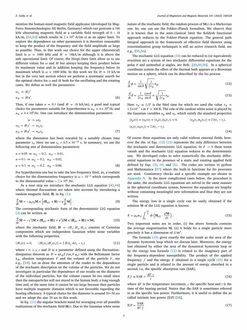
one expects the same type of function for the oscillating and rotatingcases but shifted by a factor of two, see Fig. 14. Indeed, on Fig. 14we show the SAR as a function of the ratio 𝑟 and one finds a singlemaximum for the rotating and oscillating cases where the positions ofthe peaks are related to each other, 𝑟(osc)opt = 2 𝑟(rot)opt . This demonstratesthat in order to achieve the same heating efficiency, i.e., the same SARfor the rotating and oscillating cases, one has to double the appliedfrequency (more precisely the ratio 𝑟) of the rotating applied fieldcompared to the oscillating one, so, in this case the SAR functionscoincide, see the inset of Fig. 14.
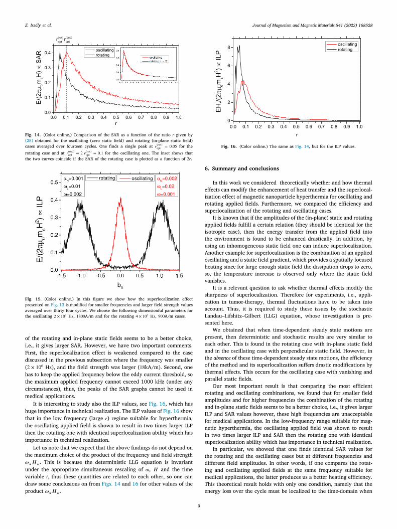
The peaks suggest optimal choices for the applied frequency andfield strength (amplitude) for the oscillating (2 × 10⁷ Hz, 1800A/m)and for the rotating (4 × 10⁷ Hz, 900A/m) cases. At these values,the SAR’s and ILP’s are the same, see Fig. 15. One finds identicalSAR and ILP values for the rotating and the oscillating cases but atdifferent frequencies and different field amplitudes. In particular, forsmaller field amplitudes and for higher frequencies the combination
Journal of Magnetism and Magnetic Materials 541 (2022) 168528Z. Iszály et al.
Fig. 14. (Color online.) Comparison of the SAR as a function of the ratio 𝑟 given by(28) obtained for the oscillating (zero static field) and rotating (in-plane static field)cases averaged over fourteen cycles. One finds a single peak at 𝑟(rot)opt = 0.05 for therotating case and at 𝑟(osc)opt = 2 𝑟(rot)opt = 0.1 for the oscillating one. The inset shows thatthe two curves coincide if the SAR of the rotating case is plotted as a function of 2𝑟.
Fig. 15. (Color online.) In this figure we show how the superlocalization effectpresented on Fig. 13 is modified for smaller frequencies and larger field strength valuesaveraged over thirty four cycles. We choose the following dimensionful parameters forthe oscillating 2 × 10⁷ Hz, 1800A/m and for the rotating 4 × 10⁷ Hz, 900A/m cases.
of the rotating and in-plane static fields seems to be a better choice,i.e., it gives larger SAR. However, we have two important comments.First, the superlocalization effect is weakened compared to the casediscussed in the previous subsection where the frequency was smaller(2 × 10⁶ Hz), and the field strength was larger (18kA/m). Second, onehas to keep the applied frequency below the eddy current threshold, sothe maximum applied frequency cannot exceed 1000 kHz (under anycircumstances), thus, the peaks of the SAR graphs cannot be used inmedical applications.
It is interesting to study also the ILP values, see Fig. 16, which hashuge importance in technical realization. The ILP values of Fig. 16 showthat in the low frequency (large 𝑟) regime suitable for hyperthermia,the oscillating applied field is shown to result in two times larger ILPthen the rotating one with identical superlocalization ability which hasimportance in technical realization.
Let us note that we expect that the above findings do not depend onthe maximum choice of the product of the frequency and field strength𝜔⋆𝐻⋆. This is because the deterministic LLG equation is invariantunder the appropriate simultaneous rescaling of 𝜔, 𝐻 and the timevariable 𝑡, thus these quantities are related to each other, so one candraw some conclusions on from Figs. 14 and 16 for other values of theproduct 𝜔 𝐻 .
9
⋆ ⋆
Fig. 16. (Color online.) The same as Fig. 14, but for the ILP values.
6. Summary and conclusions
In this work we considered theoretically whether and how thermaleffects can modify the enhancement of heat transfer and the superlocal-ization effect of magnetic nanoparticle hyperthermia for oscillating androtating applied fields. Furthermore, we compared the efficiency andsuperlocalization of the rotating and oscillating cases.
It is known that if the amplitudes of the (in-plane) static and rotatingapplied fields fulfill a certain relation (they should be identical for theisotropic case), then the energy transfer from the applied field intothe environment is found to be enhanced drastically. In addition, byusing an inhomogeneous static field one can induce superlocalization.Another example for superlocalization is the combination of an appliedoscillating and a static field gradient, which provides a spatially focusedheating since for large enough static field the dissipation drops to zero,so, the temperature increase is observed only where the static fieldvanishes.
It is a relevant question to ask whether thermal effects modify thesharpness of superlocalization. Therefore for experiments, i.e., appli-cation in tumor-therapy, thermal fluctuations have to be taken intoaccount. Thus, it is required to study these issues by the stochasticLandau–Lifshitz–Gilbert (LLG) equation, whose investigation is pre-sented here.
We obtained that when time-dependent steady state motions arepresent, then deterministic and stochastic results are very similar toeach other. This is found in the rotating case with in-plane static fieldand in the oscillating case with perpendicular static field. However, inthe absence of these time-dependent steady state motions, the efficiencyof the method and its superlocalization suffers drastic modifications bythermal effects. This occurs for the oscillating case with vanishing andparallel static fields.
Our most important result is that comparing the most efficientrotating and oscillating combinations, we found that for smaller fieldamplitudes and for higher frequencies the combination of the rotatingand in-plane static fields seems to be a better choice, i.e., it gives largerILP and SAR values however, these high frequencies are unacceptablefor medical applications. In the low-frequency range suitable for mag-netic hyperthermia, the oscillating applied field was shown to resultin two times larger ILP and SAR then the rotating one with identicalsuperlocalization ability which has importance in technical realization.
In particular, we showed that one finds identical SAR values forthe rotating and the oscillating cases but at different frequencies anddifferent field amplitudes. In other words, if one compares the rotat-ing and oscillating applied fields at the same frequency suitable formedical applications, the latter produces us a better heating efficiency.This theoretical result holds with only one condition, namely that theenergy loss over the cycle must be localized to the time-domain when
Journal of Magnetism and Magnetic Materials 541 (2022) 168528Z. Iszály et al.
a[drbot
ctotFacptaspmpTwoeacwmapo
C
atraoipaF
D
ci
A
iPgoFa
A
ndot
𝐇
wf(
vw
dv
2Fu
A
Locei
𝜒
the applied field starts to increase from its zero value, so thus theappropriate combination of rotating and (in-plane) static fields acts likean oscillating one.
In summary, we demonstrated that the combination of static androtating fields can have importance in technical realization of magneticnanoparticle hyperthermia but keeping in mind that it has a worse heat-ing efficiency compared to the usual oscillating one in the frequencyrange suitable for medical applications.
Of course, in order to look for the most efficient applied fieldconfiguration, one can perform further theoretical investigations. Forexample, open questions motivated by the present theoretical study ofthe enhancement and superlocalization effects are the inclusion of (i)the interaction between the particles which can results in formation ofclusters [60]; (ii) the dependence on the diameter of the nanoparticles;nd (iii) the possible rotating motions of the nanoparticle as a whole35,36,61–65]. However, we do expect that considerations very likelyo not violate our major finding that appropriate combination ofotating and (in-plane) static fields is essentially like an oscillating oneut in order to achieve the same heating efficiency, i.e., the same SARne has to double the applied frequency, so, for the same frequency,he oscillating combination is a better choice.
Based on our results, we suggest targeted experimental studies in-orporating standardized techniques [66,67]. For example, we proposeo use well separated isotropic nanoparticles in an aerogel matrix wherenly the magnetic moment can rotate. There are proposals for theechnical realization of a rotating applied field, see, e.g., [34] and [68].or example, in [34] the authors discuss possible experimental re-lization of generating a rotating applied field. The standard choiceould be a system of two pairs of Helmholtz coils whose axes areerpendicular to each other but in [34] the authors suggest a system ofhree pairs of inductors connected in series with capacitors to generate
rotary magnetic field. This configuration (with the inclusion of atatic field) can be directly used to test theoretical predictions of theresent work. Also non-calorimetric techniques [69,70] are used toeasure the energy losses in various applied fields. In [68], the authorsresent the validation of a resonators with a so-called birdcage coil.his represents another realization of rotating magnetic field. Again,ith the inclusion of a static field on can test our numerical resultsbtained for the rotating field case. In addition, one can discuss possiblexperimental realization to measure the decrease of heat generation asfunction of the static field. For example, a possible measurement setupould be when a rotatable resonator is placed into the electromagnethich generates the static field. In this manner, one can easily performeasurements for the case when the oscillating field and the static one
re perpendicular or parallel to each other. Thus, the predictions of theresent work can be tested with the help of the required combinationsf static and alternating applied fields.
RediT authorship contribution statement
Zs. Iszály: Data collection (numerical results, codes), Data analysisnd interpretation, Critical revision of the article, Final approval ofhe version to be published. I.G. Márián: Data collection (numericalesults, codes), Data analysis and interpretation, Critical revision of therticle. I.A. Szabó: Data analysis and interpretation, Final approvalf the version to be published. A. Trombettoni: Data analysis andnterpretation, Drafting the article, Final approval of the version to beublished. I. Nándori: Conception or design of the work, Data analysisnd interpretation, Drafting the article, Critical revision of the article,inal approval of the version to be published.
eclaration of competing interest
The authors declare that they have no known competing finan-ial interests or personal relationships that could have appeared to
10
nfluence the work reported in this paper.
cknowledgment
The CNR/MTA Italy–Hungary 2019–2021 Joint Project ‘‘Stronglynteracting systems in confined geometries’’ is gratefully acknowledged.artially supported by the ÚNKP-20-4-I New National Excellence Pro-ram of the Ministry for Innovation and Technology from the sourcef the National Research, Development and Innovation Fund, Italy.ruitful discussions with Giacomo Gori and Stefano Ruffo are gratefullycknowledged.
ppendix A. Consistency checks of the stochastic LLG equation
In this Appendix we present some consistency checks based on theumerical results discussed [50]. In Section 6 of [50] the magnetizationynamics of an anisotropic nanoparticle has been studied in the absencef any applied field and the anisotropy field is assumed to be parallelo the 𝑧-axis (by using uniaxial shape anisotropy):
eff = 𝐇a = 𝐻 (0, 0, 𝜆eff𝑀𝑧), (A.1)
here 𝜆eff = 𝐻𝑎∕𝐻 is the anisotropy ratio and 𝐻𝑎 is the anisotropyield. In the spherical coordinate system the stochastic LLG equation10) takes the form
dd𝑡𝜙 = −𝜔𝐿𝜆eff cos 𝜃 +
1sin 𝜃
√
12𝜏𝑁
𝑛𝜙, (A.2)
dd𝑡𝜃 = −𝛼𝑁𝜆eff cos 𝜃 sin 𝜃 +
12𝜏𝑁
cos 𝜃sin 𝜃
+
√
12𝜏𝑁
𝑛𝜃 , (A.3)
where 𝑛𝜙 and 𝑛𝜃 satisfy the relations given in (14). The above stochasticdifferential equations are identical to Eq. (27) of [50]. To have a moreclear picture, these can be rewritten to the standard form of an Itoprocess d𝑋 = 𝑏(𝑋) d𝑡 + 𝜎 d𝑊 . From (14) one can observe that theariance of 𝑛𝜙(𝜃) is multiplied by a factor of 2, which can be explicitlyritten as a
√
2 multiplicative factor of the Wiener process. Thus thefull stochastic process in the standard form writes as
d𝜙 = −𝜔𝐿𝜆eff cos 𝜃 d𝑡 + 1sin 𝜃
√
12𝜏𝑁
√
2 d𝑊1, (A.4)
d𝜃 =(
−𝛼𝑁𝜆eff cos 𝜃 sin 𝜃 +1
2𝜏𝑁cos 𝜃sin 𝜃
)
d𝑡 +
√
12𝜏𝑁
√
2 d𝑊2, (A.5)
where d𝑊1 and d𝑊2 are independent Wiener processes with the stan-dard normal distribution. This Ito process can be directly solved by thebuilt-in functions of Mathematica [57], where the time is discretized.In this case setting the numerical time step d𝑡 = 1.5 × 10⁻¹⁰ s producesreliable results. At each time step, d𝜙 and d𝜃 receives a random, normalistributed ‘kick’ from the d𝑊 terms centered around zero with aariance that is adjusted by the size of the time step 𝜎2𝑊 = d𝑡. Fig. 6
of Ref. [50] contains some details regarding the average values ofthe Cartesian components of the magnetization vector. Therefore itis illustrative to recover this known result by our stochastic solverusing the same values for the parameters 𝜏𝑁 = 1.5 × 10⁻⁷ s, 𝜔𝐿𝜆eff =.58×108 s−1, 𝛼𝑁𝜆eff = 7.74×10⁷ s−1, results from which are presented inig. 17. The comparison confirms the validity of the numerical methodsed here for the stochastic solver.
ppendix B. Consistency check of the results
In order to check our theoretical results based on the stochasticLG equation, we determine the imaginary part of the AC susceptibilitybtained for the pure oscillating (without static) external field andompare it to the corresponding literature both on the theory and thexperimental side. The frequency dependence of the AC susceptibilitys given by′′(𝜔) = 𝜒 𝜔𝜏 (B.1)
0 1 + 𝜔2𝜏2
Journal of Magnetism and Magnetic Materials 541 (2022) 168528Z. Iszály et al.
wit
ttrf
LI𝜏sk
R
Fig. 17. In this figure we plot the average values of 𝑀𝑥(𝑡) (green curve), 𝑀𝑦(𝑡) (yellowcurve) and 𝑀𝑧(𝑡) (blue curve) are plotted versus the time where the horizontal red linestands for the asymptotic value given in Ref. [50] (compare it in particular with thecentral panel of Fig. 6 in Ref. [50]).
Fig. 18. (Color online.) In this figure we plot the imaginary parts of the ACsusceptibility (which is related to ILP) as a function of the applied (dimensionless)frequency for pure oscillating case. Numerical data are identical to the red curve ofFig. 11. The solid line is a fitted curve to numerical data based on (B.1).
see for example Eq.(4) and (5) of [70]. This form is valid when asingle relaxation process is present only. In our case the frequencydependence is characterized by the Néel relaxation time, 𝜏 = 𝜏𝑁 , since
e investigated small enough nanoparticles to neglect their rotationnside their environment and only the Néel process, i.e, the rotation ofhe magnetization is taken into count.
We use the formula (B.1) to fit our theoretical results obtained byhe stochastic LLG equation for the pure oscillating case. On Fig. 18he solid line denotes the fitted curve which gives the following fittedelaxation time, 𝜏𝑁 = 157×0.5×10−10 s ∼ 0.78×10⁻⁸ s and the followingitted magnitude, 𝜒0 = 1.09.
We conclude that our numerical results obtained by the stochasticLG equation can be well described by the standard formula (B.1).n addition, the relaxation time calculated by the fitting procedure,𝑁 ∼ 1 ns is in the range of typical value for magnetic nanoparticles,ee e.g., [71]. Finally, we argue that our results are in agreement withnown experimental results, see for example, Fig. 2 of [72].
eferences
[1] Q.A. Pankhurst, J. Connolly, S.K. Jones, J. Dobson, Applications of magneticnanoparticles in biomedicine, J. Phys. D: Appl. Phys. 36 (2003) R167.
[2] D. Ortega, Q.A. Pankhurst, Magnetic hyperthermia, Nanoscience 1 (2003) e88.[3] Q.A. Pankhurst, N.T.K. Thanh, S.K. Jones, J. Dobson, Progress in applications
of magnetic nanoparticles in biomedicine, J. Phys. D: Appl. Phys. 42 (2003)
11
224001.
[4] E.A. Perigo, G. Hemery, O. Sandre, D. Ortega, E. Garaio, F. Plazaola, F.J. Teran,Fundamentals and advances in magnetic hyperthermia, Appl. Phys. Rev. 2 (2015)041302.
[5] D. Cabrera, J. Camarero, D. Ortega, F.J. Teran, Influence of the aggregation,concentration, and viscosity on the nanomagnetism of iron oxide nanoparticlecolloids for magnetic hyperthermia, J. Nanopart. Res. 17 (2015) 121.
[6] B. Thiesen, A. Jordan, Clinical applications of magnetic nanoparticles forhyperthermia, Int. J. Hyperth. 24 (2008) 467–474.
[7] P. Wust, U. Gneveckow, M. Johannsen, et al., Magnetic nanoparticles forinterstitial thermotherapy, feasibility, tolerance and achieved temperatures, Int.J. Hyperth. 22 (2006) 673–685.
[8] M. Creixell, A.C. Bohorquez, M. Torres-Lugo, C. Rinaldi, EGFR-targeted magneticnanoparticle heaters kill cancer cells without a perceptible temperature rise, ACSNano 5 (2011) 7124.
[9] M. Domenech, I. Marrero-Berrios, M. Torres-Lugo, C. Rinaldi, Lysosomalmembrane permeabilization by targeted magnetic nanoparticles in alternatingmagnetic fields, ACS Nano 7 (2013) 5091–5101.
[10] A. Chiu-Lam, C. Rinaldi, Nanoscale thermal phenomena in the vicinity ofmagnetic nanoparticles in alternating magnetic fields, Adv. Funct. Mater. 26(2016) 3933–3941.
[11] C. Weber, S. Morsbach, K. Landfester, Possibilities and limitations of differentseparation techniques for the analysis of the protein corona, Angew. Chem. 58(2019) 12787–12794.
[12] R. Dhavalikar, A.C. Bohorquez, C. Rinaldi, Image-guided thermal therapy usingmagnetic particle imaging and magnetic fluid hyperthermia, in: Nanomate-rials for Magnetic and Optical Hyperthermia Applications, Micro and NanoTechnologies, 2019, pp. 265–286.
[13] C. Kut, Y. Zhang, M. Hedayati, H. Zhou, C. Cornejo, D. Bordelon, J. Mihalic, M.Wabler, E. Burghardt, C. Gruettner, A. Geyh, C. Brayton, T.L. Deweese, R. Ivkov,Preliminary study of injury from heating systemically delivered, nontargeteddextran superparamagnetic iron oxide nanoparticles in mice, Nanomedicine 7(2012) 1697.
[14] Z.W. Tay, P. Chandrasekharan, A. Chiu-Lam, D.W. Hensley, R. Dhavalikar, X.Y.Zhou, E.Y. Yu, P.W. Goodwill, B. Zheng, C. Rinaldi, S.M. Conolly, Magneticparticle imaging-guided heating in vivo using gradient fields for arbitrarylocalization of magnetic hyperthermia therapy, ACS Nano 12 (2018) 3699–3713.
[15] T.O. Tasci, I. Vargel, A. Arat, E. Guzel, P. Korkusuz, E. Atalar, Focused RFhyperthermia using magnetic fluids, Med. Phys. 36 (2009) 1906–1912.
[16] S.L. Ho, L. Jian, W. Gong, W.N. Fu, Design and analysis of a novel targetedmagnetic fluid hyperthermia system for tumor treatment, IEEE Trans. Magn. 48(2012) 3262–3265.
[17] S.L. Ho, S. Niu, W.N. Fu, Design and analysis of novel focused hyperthermiadevices, IEEE Trans. Magn. 48 (2012) 3254–3257.
[18] M. Ma, Y. Zhang, X. Shen, J. Xie, Y. Li, N. Gu, Targeted inductive heating ofnanomagnets by a combination of alternating current (AC) and static magneticfields, Nano Res. 8 (2015) 600–610.
[19] D.W. Hensley, Z.W. Tay, R. Dhavalikar, B. Zheng, P. Goodwill, C. Rinaldi, S.Conolly, Combining magnetic particle imaging and magnetic fluid hyperthermiain a theranostic platform, Phys. Med. Biol. 62 (2017) 3483.
[20] R. Dhavalikar, C. Rinaldi, Theoretical predictions for spatially-focused heating ofmagnetic nanoparticles guided by magnetic particle imaging field gradients, J.Magn. Magn. Mater. 419 (2016) 267–273.
[21] Zs. Iszály, K. Lovász, I. Nagy, I.G. Márián, J. Rácz, I.A. Szabó, L. Tóth, N.F. Vas,V. Vékony, I. Nándori, Efficiency of magnetic hyperthermia in the presence ofrotating and static fields, J. Magn. Magn. Mater. 466 (2018) 452–462.
[22] M.-K. Kim, J. Sim, J.-H. Lee, M. Kim, S.-K. Kim, Dynamical origin of highly effi-cient energy dissipation in soft magnetic nanoparticles for magnetic hyperthermiaapplications, Phys. Rev. Appl. 9 (2018) 054037.
[23] G. Bertotti, C. Serpico, I.D. Mayergoyz, Nonlinear magnetization dynamics undercircularly polarized field, Phys. Rev. Lett. 86 (2001) 724.
[24] S.I. Denisov, T.V. Lyutyy, P. Hänggi, Magnetization of nanoparticle systems in arotating magnetic field, Phys. Rev. Lett. 97 (2006) 227202.
[25] S.I. Denisov, T.V. Lyutyy, P. Hänggi, K.N. Trohidou, Dynamical and thermaleffects in nanoparticle systems driven by a rotating magnetic field, Phys. Rev. B74 (2006) 104406.
[26] P. Cantillon-Murphy, L.L. Wald, E. Adalsteinsson, M. Zahn, Heating in the MRIenvironment due to superparamagnetic fluid suspensions in a rotating magneticfield, J. Magn. Magn. Mater. 322 (2010) 727–733.
[27] O.O. Ahsen, U. Yilmaz, M.D. Aksoy, G. Ertas, E. Atalar, Heating of magnetic fluidsystems driven by circularly polarized magnetic field, J. Magn. Magn. Mater. 322(2010) 3053–3059.
[28] Yu.L. Raikher, V.I. Stephanov, Power losses in a suspension of magnetic dipolesunder a rotating field, Phys. Rev. E 83 (2011) 021401.
[29] S.I. Denisov, T.V. Lyutyy, C. Binns, P. Hänggi, Phase diagrams for the precessionstates of the nanoparticle magnetization in a rotating magnetic field, J. Magn.Magn. Mater. 322 (2010) 1360–1362.
[30] S.I. Denisov, A.Yu. Polyakov, T.V. Lyutyy, Resonant suppression of thermalstability of the nanoparticle magnetization by a rotating magnetic field, Phys.Rev. B 84 (2011) 174410.
Journal of Magnetism and Magnetic Materials 541 (2022) 168528Z. Iszály et al.
[31] T.V. Lyutyy, S.I. Denisov, A.Yu. Polyakov, C. Binns, Power loss of the nanopar-ticle magnetic moment in alternating fields, in: Nanomaterials: Applications andProperties (NAP-2012): 2-nd International Conference, Vol. 1, 2012, 04MFPN16.
[32] T.V. Lyutyy, S.I. Denisov, A.Yu. Peletskyi, C. Binns, Energy dissipation in single-domain ferromagnetic nanoparticles: Dynamical approach, Phys. Rev. B 91(2015) 054425.
[33] S.-W. Chen, J.-J. Lai, C.-L. Chiang, C.-L. Chen, Construction of orthogonalsynchronized bi-directional field to enhance heating efficiency of magneticnanoparticles, Rev. Sci. Instrum. 83 (2012) 064701.
[34] A. Skumiel, B. Leszczynski, M. Molcan, M. Timko, The comparison of magneticcircuits used in magnetic hyperthermia, J. Magn. Magn. Mater. 420 (2016)177–184.
[35] T.V. Lyutyy, O.M. Hryshko, A.A. Kovner, Power loss for a periodically drivenferromagnetic nanoparticle in a viscous fluid: The finite anisotropy aspects, J.Magn. Magn. Mater. 446 (2018) 87–94.
[36] N.A. Usov, R.A. Rytov, V.A. Bautin, Dynamics of superparamagnetic nanoparti-cles in viscous liquids in rotating magnetic fields, Beilstein J. Nanotechnol. 10(2019) 2294.
[37] P.T. Phong, L.H. Nguyen, I.J. Lee, N.X. Phuc, Computer simulations of contribu-tions of Néel and Brown relaxation to specific loss power of magnetic fluids inhyperthermia, J. Electron. Mater. 46 (2017) 2393–2405.
[38] R. Hergt, S. Dutz, M. Zeisberger, Validity limits of the Néel relaxation model ofmagnetic nanoparticles for hyperthermia, Nanotechnology 21 (2010) 015706.
[39] R. Hergt, W. Andra, C. d’Ambly, I. Hilger, W. Kaiser, U. Richter, H. Schmidt,Physical limits of hyperthermia using magnetite fine particles, IEEE Trans. Magn.34 (1998) 3745.
[40] R. Hergt, S. Dutz, Magnetic particle hyperthermia: biophysical limitations of avisionary tumour therapy, J. Magn. Magn. Mater. 311 (2007) 187–192.
[41] L. Landau, E. Lifshitz, On the theory of the dispersion of magnetic permeabilityin ferromagnetic bodies, Phys. Z. Sowjetunion 8 (1935) 153.
[42] T.L. Gilbert, A Lagrangian formulation of the gyromagnetic equation of themagnetization field, Phys. Rev. 100 (1955) 1243.
[43] W.F. Brown, Thermal fluctuations of a single-domain particle, Phys. Rev. 130(1963) 1677.
[44] W. Brown, Thermal fluctuation of fine ferromagnetic particles, IEEE Trans. Magn.15 (1979) 1196–1208.
[45] P.C. Fannin, I. Malaescue, C.N. Marin, The effective anisotropy constant ofparticles within magnetic fluids as measured by magnetic resonance, J. Magn.Magn. Mater. 289 (2005) 162–164.
[46] Let us note Eq. (1) is identical to Eq. (2.1) of [54], where 𝐌 denotes the un-normalised magnetization (so, in Ref. [54] 𝐌 is not a unit vector and in additionone has to make the following replacement 𝛾0 → 𝜇0𝛾0). Furthermore, Eq. (1) isidentical to Eqs. (1) and (4) of Ref. [49].
[47] I. Nándori, J. Rácz, Magnetic particle hyperthermia: Power losses under circularlypolarized field in anisotropic nanoparticles, Phys. Rev. E 86 (2012) 061404.
[48] P.F. de Châtel, I. Nándori, J. Hakl, S. Mészáros, K. Vad, Magnetic particle hy-perthermia: Néel relaxation in magnetic nanoparticles under circularly polarizedfield, J. Phys.: Condens. Matter 21 (2009) 124202.
[49] J. Rácz, P.F. de Châtel, I.A. Szabó, L. Szunyogh, I. Nándori, Improved efficiencyof heat generation in nonlinear dynamics of magnetic nanoparticles, Phys. Rev.E 93 (2016) 012607.
[50] S. Giordano, Y. Dusch, N. Tiercelin, P. Pernod, V. Preobrazhensky, Stochasticmagnetization dynamics in single domain particles, Eur. Phys. J. B 86 (2013)249.
[51] D. Bordelon, C. Cornejo, C. Grüttner, F. Westphal, T.L. DeWeese, R. Ivkov,Magnetic nanoparticle heating efficiency reveals magneto-structural differenceswhen characterized with wide ranging and high amplitude alternating magneticfields, J. Appl. Phys. 109 (2011) 124904.
12
[52] U. Gneveckow, A. Jordan, R. Scholz, V. Bruss, N. Waldofner, J. Ricke, A.Feussner, B. Hildebrandt, B. Rau, P. Wust, Description and characterization ofthe novel hyperthermia and thermoablation system for clinical magnetic fluidhyperthermia, Med. Phys. 31 (2004) 1444–1451.
[53] B. Thiesen, A. Jordan, Clinical applications of magnetic nanoparticles forhyperthermia, Int. J. Hyperth. 24 (2008) 467–474.
[54] C. Aron, D.G. Barci, L.F. Cugliandolo, Z.G. Arenas, G.S. Lozano, Magnetiza-tion dynamics: path-integral formalism for the stochastic Landau-Lifshitz-Gilbertequation, J. Stat. Mech. (2014) P09008.
[55] S. Grozdanov, J. Polonyi, Viscosity and dissipative hydrodynamics from effectivefield theory, Phys. Rev. D 91 (2015) 105031.
[56] S. Nagy, J. Polonyi, I. Steib, Quantum renormalization group, Phys. Rev. D 93(2016) 025008.
[57] Wolfram Research, Inc., Mathematica, Champaign, IL, 2021.[58] M. Kallumadil, M. Tada, T. Nakagawa, M. Abe, P. Southern, Q.A. Pankhurst,
Suitability of commercial colloids for magnetic hyperthermia, J. Magn. Magn.Mater. 321 (2009) 1509–1513.
[59] N.A. Usov, Low frequency hysteresis loops of superparamagnetic nanoparticleswith uniaxial anisotropy, J. Appl. Phys. 107 (2010) 123909.
[60] N.A. Usov, O.N. Serebryakova, V.P. Tarasov, Interaction effects in assembly ofmagnetic nanoparticles, Nanoscale Res. Lett. 12 (2017) 489.
[61] H. Mamiya, B. Jeyadevan, Hyperthermic effects of dissipative structures ofmagnetic nanoparticles in large alternating magnetic fields, Sci. Rep. 1 (2011)157.
[62] N.A. Usov, B.Y. Liubimov, Dynamics of magnetic nanoparticle in a viscous liquid:Application to magnetic nanoparticle hyperthermia, J. Appl. Phys. 112 (2012)023901.
[63] N.A. Usov, B.Y. Liubimov, Magnetic nanoparticle motion in external magneticfield, J. Magn. Magn. Mater. 385 (2015) 339–346.
[64] K.D. Usadel, C. Usadel, Dynamics of magnetic single domain particles embeddedin a viscous liquid, J. Appl. Phys. 118 (2015) 234303.
[65] T.V. Lyutyy, V.V. Reva, Energy dissipation of rigid dipoles in a viscous fluidunder the action of a time-periodic field: The influence of thermal bath anddipole interaction, Phys. Rev. E 97 (2018) 052611.
[66] J. Wells, D. Ortega, U. Steinhoff, S. Dutz, E. Garaio, O. Sandre, E. Na-tividad, M.M. Cruz, F. Brero, P. Southern, Q.A. Pankhurst, S. Spassov,and the RADIOMAG consortium, Challenges and recommendations for mag-netic hyperthermia characterization measurements, Int. J. Hyperth. 38 (2021)447–460.
[67] R.R. Wildeboer, P. Southern, Q.A. Pankhurst, On the reliable measurement ofspecific absorption rates and intrinsic loss parameters in magnetic hyperthermiamaterials, J. Phys. D: Appl. Phys. 47 (2014) 495003.
[68] I. Gresits, Gy. Thuróczy, O. Sági, B. Gyüre-Garami, B.G. Márkus, F. Simon,Non-calorimetric determination of absorbed power during magnetic nanoparticlebased hyperthermia, Sci. Rep. 8 (2018) 12667.
[69] I. Gresits, Gy. Thuróczy, O. Sági, I. Homolya, G. Bagaméry, D. Gajári, M. Babos,P. Major, B.G. Márkus, F. Simon, A highly accurate determination of absorbedpower during magnetic hyperthermia, J. Phys. D: Appl. Phys. 52 (2019) 375401.
[70] I. Gresits, Gy. Thuróczy, O. Sági, S. Kollarics, G. Csősz, B.G. Márkus, N.M. Nemes,M. García Hernández, F. Simon, Non-exponential magnetic relaxation in magneticnanoparticles for hyperthermia, J. Magn. Magn. Mater. 526 (2021) 167682.
[71] Satoshi Ota, Yasushi Takemura, J. Phys. Chem. C 123 (2019) 28859.[72] R.M. Ferguson, et al., IEEE Trans. Magn. 49 (2013) 3441.