Thermal analysis of cooling curves for

phase diagram determination

1P6 Thermal Analysis

Updated: 2020-01-28

Senior Demonstrator: Dr Enzo Liotti

Junior Demonstrator: Ms Ceren Zor

Safety

Hazards Control measures

High temperature

molten metal

Safety glasses and lab coat must be worn throughout

entire time when in the lab.

Lab coat, safety glasses and visor, thermal resistant

gloves, aprons and shoe protector are worn when

working in the furnace room.

Follow instructions, training and supervision.

Incorrect operation

of furnaces Follow instructions, training and supervision.

Safety Rules:

Demonstrators must be present when you are working with molten metal.

Request permission from the demonstrators before operating the furnaces.

The furnaces and temperature inside the sample tube must not be allowed to

go above 300C.

Listen and follow instructions carefully. If you do not understand instructions,

then ask before you perform the tasks.

1P6 – Thermal Analysis

2

Contents

1. Objectives and Learning Outcomes ...................................................................................... 3

1.1. Objectives and Science .................................................................................................... 3

1.2. Practical Skills.................................................................................................................. 3

1.3. Computer Skills ............................................................................................................... 4

2. Overview of the Practical ....................................................................................................... 4

2.1. Practical Timetable .......................................................................................................... 5

2.2. List of files ........................................................................................................................ 5

3. Experimental Method ............................................................................................................. 6

3.1. Measuring Heating and Cooling Curves ....................................................................... 6

3.2. Task 1 ................................................................................................................................ 6

3.3. Task 2 ................................................................................................................................ 8

3.4. Task 3 ................................................................................................................................ 9

3.5. Operating the Furnaces................................................................................................... 9

3.6. Preparing Sample Hn ..................................................................................................... 10

4. Data Analysis ......................................................................................................................... 10

5. Laboratory Report ................................................................................................................ 11

5.1. Structure ......................................................................................................................... 11

5.2. Length ............................................................................................................................. 12

5.3. Marking Considerations ............................................................................................... 13

1P6 – Thermal Analysis

3

1. Objectives and Learning Outcomes

1.1. Objectives and Science

The overall objective of this practical is to demonstrate how a phase diagram of an

alloy system can be obtained experimentally. The second objective is to learn how

to use latest software techniques, such as LabView (Laboratory Virtual Instrument

Engineering Workbench) and MATLAB (MATrix LABoratory), to collect, organise

and analyse scientific data. This practical links with the lecture courses on

thermodynamics and microstructures.

In this practical, an alloy system will be studied, by analyzing the cooling curves of

samples with different composition, and its phase diagram determined. The cooling

curves will reveal the beginning and end of solidification, pure metals and eutectics

freeze at one temperature whereas other compositions within a range. The Phase Rule

model predicts this phenomenon.

The practical involves the development of both practical and computing skills

essential to become a successful material scientist.

1.2. Practical Skills

The work will involve the measurement, interpretation of cooling curves, and

producing an alloy of uniform composition. It is expected that the practical will

involve:

Operate a simple tube furnace;

Learn how to handle molten metals safely;

Learn how to set up equipment to conduct simple measurements;

Understand the basic working principles of thermocouples and use them to

measure the temperature of a sample;

1P6 – Thermal Analysis

4

1.3. Computer Skills

Use LabView to control hardware equipment and record temperatures;

Use MATLAB to import datasets and develop a script that analyses the data.

2. Overview of the Practical

On Day 1 you will find eight tube furnaces loaded with prepared samples all from

the same X-Y alloy system. During the practical you will prepare the experimental

set up, test the eight samples and also be given the data of a ninth sample to analyse

while the experiment is running. The nine prepared samples are: one of unknown

pure element X, one of unknown pure element Y (not Yttrium) and the others are

alloys with various compositions, as given in the Table 1.

Sample Composition (wt%)

A 100X

B 97X – 3Y

C 90X – 10Y

D 70X – 30Y

E 60X – 40Y

F 48X – 52Y

G 30X – 70Y

H 11X – 89Y

I 100Y

Table 1: Summary of all sample compositions.

Working as a group, you will record the heating and cooling curves of one of these

prepared samples and share the data with the other groups. The datasets will be

analysed using MATLAB and the results used to construct the phase diagram for the

X-Y system.

In addition, on Day 1 each group will also choose a composition to make their own

sample Hn, where n is your group number, which will be tested on Day 2. The dataset

(but not the compositions) will be shared with the other groups, and using the phase

1P6 – Thermal Analysis

5

diagram constructed from the results of the analysis of the samples in table 1, you

will determine the composition of all the other groups’ Hn alloys. The practical

overall expected results are:

- X-Y phase diagram;

- Identification of the alloy system from the constructed phase diagram;

- Identification of all the Hn sample compositions;

2.1. Practical Timetable

Day 1:

1. Set up furnaces and measuring equipment;

2. Measurement of heating and cooling curves for the prepared sample;

3. Preparation of alloy Hn of composition ___%X and ___%Y;

4. Preliminary MATLAB data analysis of sample E.

Day 2:

1. Measurement of heating and cooling curves for your alloy Hn;

2. Analysis of datasets from Day 1 samples, including those from other groups;

3. Determination of phase diagram;

2.2. List of files

The practical involves the use of several files, which are found in the folder

“Practical_1P6_Thermal analysis” on the desktop of the shared laptop connected to

the furnaces. The folder contains the following files and subfolders:

- DataAcquisition_LabView: this folder contains all the necessary files to run

the LabView user interface to record the heating and cooling curves;

- “NI USB 9211a manual.pdf”: manual for the NI module;

- “s_ThermalAnalysis_1P6.m”: Matlab script to be used to analyse the heating

and cooling curves;

- Sample E data file;

1P6 – Thermal Analysis

6

3. Experimental Method

3.1. Measuring Heating and Cooling Curves

For this practical, each group is provided with one manually controlled tube furnace,

a shared laptop running LabView for data acquisition and shared data logging

hardware. There are four data logging units each of them connected to a laptop and

recording the temperature of two experiments. The data logging is carried out using

the National Instrument hardware and software: a NI 9211 thermocouple module,

which read a voltage and convert it to temperature, is connected to a laptop via a

cDAQ-9171 USB module. The module enables the communication between the

thermocouple module and the computer. Each module can read 4 thermocouples

simultaneously and it is controlled by LabView.

The temperatures will be recorded using thermocouples provided. Thermocouples

are electrical device consisting of two dissimilar conductors forming electrical

junctions at differing temperatures. A temperature-dependent voltage is produced as

a result of the thermoelectric effect, and this voltage can be interpreted to measure

temperature. There are several types of thermocouples differing in the combination

of the alloys employed; in this experiment, we will use K-type thermocouples

(chromel-alumen), which are well suited for measuring temperatures of non-reactive

molten metals in the range −200 °C to +1350 °C.

3.2. Task 1

On Day 1, the specimens will have been made up already in crucibles and loaded

into the tube furnace, but you will have to set up the data logging equipment and

modify the given LabView code in order to be able to start the experiment.

As a first task connect the thermocouples to the module, remember that they have a

positive and a negative end and that polarity is important so attach them the right

way around! (Hint: thermocouples wire colors are standard, google knows the

answer, but you must ask the right question…).

1P6 – Thermal Analysis

7

When all the thermocouples are connected, launch LabView and open the file

“Thermocouple Data Acquisition_v2.vi”, which is in the folder named

“DataAcquisition_Labview” within the practical main folder. The program window

is the front panel of the code, which was written for this practical (Fig. 1). Press

Ctrl+E to open the underlying block diagram (Fig. 2).

Fig. 1: Front panel of the LabView data logging program. Press Ctrl+E to see

the block diagram. Press the run button ( ) to launch the program.

1P6 – Thermal Analysis

8

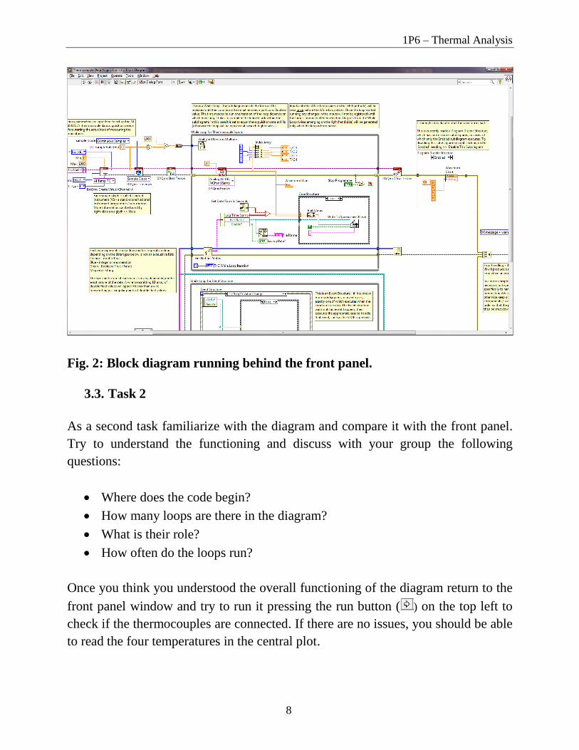
Fig. 2: Block diagram running behind the front panel.

3.3. Task 2

As a second task familiarize with the diagram and compare it with the front panel.

Try to understand the functioning and discuss with your group the following

questions:

Where does the code begin?

How many loops are there in the diagram?

What is their role?

How often do the loops run?

Once you think you understood the overall functioning of the diagram return to the

front panel window and try to run it pressing the run button ( ) on the top left to

check if the thermocouples are connected. If there are no issues, you should be able

to read the four temperatures in the central plot.

1P6 – Thermal Analysis

9

3.4. Task 3

If you get the program working, you will notice that the acquisition rate is very low.

This was intentional and it is your next task to change it to a suitable value. To do so

you need first to find out how to reset it and then to work out which would be a

suitable acquisition rate.

Stop the program pressing the red button ‘Stop Programme’. Do not stop it in any

other way as it can cause problem of communication between the computer and the

NI modules, in which case you might have to restart LabView.

Go to the block diagram and try to identify where the sampling rate is set. When you

find it, try to reset it to another value and test if it works.

Now that you know how to correct the acquisition rate, you will then need to choose

an appropriate value for the parameter (think carefully!). (Hint: you might find some

help in the NI 9211 module manual).

3.5. Operating the Furnaces

Start the data log pressing ‘Start Log?’ and give the file a meaningful name.

Remember that each computer is reading the temperature of two experiments. Thus,

write down which channel correspond to your experiment in your lab-book.

The furnace is controlled by a Eurotherm temperature controller. Once you are ready

to operate the furnace, it is imperative that a demonstrator supervises and provides

explicit permission to switch on the furnaces.

Set the target temperature to 300oC and with the demonstrator’s permission, switch

on the controller. One group member must always remain by the equipment to

monitor the sample’s temperature. Once the temperature inside the sample tube has

reached 300oC, notify the demonstrators and they will instruct you to switch off the

furnace.

Two group members now prepare their own alloy, specimen Hn (see instructions

below), ready for analysis on Day 2. The remaining group members relocate to the

computer room to begin the MATLAB data processing (see Section 6.).

1P6 – Thermal Analysis

10

At the end of Day 1, check the temperature of the sample; if it is below 100oC, you

can stop the data logging. However, remember that a laptop is recording data from

two furnaces so check both temperatures. If the temperature is above 100oC, then

notify the demonstrators. The data from Day 1 will be collected at the beginning of

Day 2. The data from Day 2 will be collected the start of the next week. It is your

responsibility to collect the data.

3.6. Preparing Sample Hn

In order to prepare specimen Hn, you must decide on its composition. Weigh the

appropriate quantities of pure X and pure Y using the raw materials provided to give

a total weight of 100g. You should take a note of the actual weights and equipment

used (as this might be useful in your error discussion). Place X and Y together in the

supplied crucible and let the Demonstrators know you are ready for further

instructions. You must not enter the furnace room without supervision.

Under the supervision of the Demonstrators, put on protective clothing (visor, gloves

and apron). With their guidance, place the crucible into the furnace pre-heated to

350C using the long-handled tongs. Secure a glass test-tube in a retort stand ready

to receive the molten metal.

After 30 minutes, insert the thermocouple into the mold, remove the crucible

containing the molten metal and stir with a graphite rod prior to pouring the molten

metal into a glass test-tube. Allow the specimen to cool for 10 minutes. Specimen Hn

is now ready for analysis on Day 2.

4. Data Analysis

The analysis of the collected heating and cooling curves will be carried out using

MATLAB to determine the temperatures where solidification starts and finishes and

construct the phase diagram. At the end of this practical you will have the datasets

for the eight prepared samples (one of which your group will have analysed on Day

1), the group’s alloy Hn and all the other groups’ alloy Hn (which you will not know

the composition). Your group should analyse each data set as follows.

1P6 – Thermal Analysis

11

Double click the supplied MATLAB script titled ‘s_ThermalAnalysis_1P6.m’. The

script will guide you through the entire data analysis process and at the end you

should be able to construct the phase diagram.

A supplied dataset for alloy X60-Y40 (wt%) has already been provided within the

MATLAB folder. Following the instructions, start to prepare a plot of the heating

and cooling curves for this alloy, determining the temperatures where solidification

starts and finishes. Consider how this information will contribute to your

construction of the phase diagram.

5. Laboratory Report

After an experiment (whether it was successful or unsuccessful), it is important to

produce a scientific report that clearly and concisely communicate the findings.

5.1. Structure

The report should be written in a descriptive form (remember it is not a questionnaire

or a list of actions!) and be structured as a scientific journal paper (e.g. Acta

Materialia) divided in five main sections:

Introduction: Introduce the topic, clarify the motivation for the work

presented and explain the content of the next sections. It is expected that you

briefly review some of the relevant background literature (describing what

others have done before you), using citations to help the reader follow up.

Methods: This section should provide enough detail and information for

others to reproduce your experiments. It should contain information about

your samples, the experimental set up (e.g. type of furnaces, model and type

of modules used for the temperature measurements etc.), but not extensive

descriptions of the functioning of the hardware or its background science. It

should also describe the methodology utilized for the data analysis of the

presented results.

Results: Present your results objectively and report only those relevant for the

interpretation of the cooling curves, the determination of the phase diagram

1P6 – Thermal Analysis

12

and alloy system and the identification of the Hn sample compositions. It is

also acceptable that you incorporate your discussion (see next point) to the

results and use instead a “Results and discussion” section.

Discussion: This section should contains your interpretation of the results,

explaining the reader what they mean. Some speculation is acceptable,

although it should be clearly stated when not enough evidence exists to back

them up. Compare your results with the literature and with other thermal

analysis technique. Discuss the data analysis approach and compare different

data analysis methods.

Conclusions: This final section presents the outcome of the work by

summarizing the findings in a more concise way, typically in the form of bullet

points. The findings are often related to the motivation stated in the

introduction section.

References should be added at the end of the manuscript and formatted to the IEEE

standard.

5.2. Length

The report should be submitted electronically and should NOT exceed 3000 words

of text with a maximum of 10 figures. The figures should be done in MATLAB and

could be divided in subfigures (or subplots). Compulsory figures are: your phase

diagram, a figure containing an example of one of the cooling curves you used for

the determination of the phase diagram, a figure which explain the data analysis

method. References and figure captions do not contribute to the word count.

1P6 – Thermal Analysis

13

5.3. Marking Considerations

Your report will be marked out of a total of 13. The allocation of marks is as follows:

Introduction 2 marks

Description of methods used including methods of data

processing and analysis

3 marks

Presentation of results including the appropriateness of figures

and data presented, and the use of errors where appropriate

4 marks

Discussion and interpretation of results 3 marks

Conclusions 1 mark