Page 1
A Recursive approach to Floorplanning
by
Renishkumar V. Ladani
A Thesis Submitted in Partial Fulfilment of the Requirements for the Degree of
Master of Technology
in
Information and Communication Technology
to
Dhirubhai Ambani Institute of Information and Communication Technology
May, 2005
DA-IICT
Page 2
Sponsored By: Bonrix Software Systems, Ahmedabad, India.www.bonrix.net, www.bonrix.co.in
Declaration
This is to certify that
(i) the thesis comprises my original work towards the degree of Master of Technology in
Information and Communication Technology at DA-IICT and has not been submitted
elsewhere for a degree,
(ii) due acknowledgement has been made in the text to all other material used.
Renishkumar V. Ladani
i
Page 3
Sponsored By: Bonrix Software Systems, Ahmedabad, India.www.bonrix.net, www.bonrix.co.in
Certificate
This is to certify that the thesis work entitled “A Recursive Approach to Floorplanning”
has been carried out by Renishkumar V. Ladani (200311014) for the degree of Master of
Technology in Information and Communication Technology at this Institute under my
supervision.
Prof. Ashok T. Amin
Thesis Supervisor
ii
Page 4
Sponsored By: Bonrix Software Systems, Ahmedabad, India.www.bonrix.net, www.bonrix.co.in
Acknowledgements
I am thankful to my guide Prof. Ashok T. Amin for guiding me throughout my thesis
work. His suggestions and constant support during this research are motivating factor for
me. I consider myself very lucky to get an opportunity to work with him. I am thankful to
my co-guide Prof. Amit Bhatt for providing initial insight into field of floorplanning. I
am thankful to my evaluation-committee members, Prof. D. Nag Chaudhary and Prof.
Hemangi Kapoor for providing useful suggestions for my research work. I am thankful to
my colleagues and friends for motivating me for research and providing constant support
in difficult times. I am thankful to J. M. Lin and Y. W. Chang (@cc.ee.ntu.edu.tw) for
making available their floorplanning algorithm implementation and test cases on their
home page. I am thankful to Dr. Hirendu P. Vaishnav of Synapps Corp., USA for his
suggestion of floorplanning as a research topic. I am thankful to DA-IICT for providing
me the resources needed and a favourable environment to carry out my work. I am
thankful to my family for supporting me in all the ways.
iii
Page 5
Sponsored By: Bonrix Software Systems, Ahmedabad, India.www.bonrix.net, www.bonrix.co.in
Contents
Page No.
ABSTRACT........................................................................................................................................... VI
LIST OF PRINCIPAL SYMBOLS AND ACRONYMS....................................................................VII
LIST OF TABLES............................................................................................................................. VIII
LIST OF FIGURES.............................................................................................................................. IX
1. INTRODUCTION............................................................................................................................... 1
1.1 FLOORPLANNING IN CONTEXT OF VLSI PHYSICAL DESIGN.......................................................11.2 FLOORPLANNING DEFINITION...................................................................................................21.3 FLOORPLAN PROBLEM DESCRIPTION.............................................................................................3
1.3.1 Floorplan Sizing: A optimization problem in Floorplanning...............................................51.3.2 Some Constraints in Floorplanning....................................................................................5
1.4 MOTIVATION........................................................................................................................... 51.5 ORGANIZATION OF THE THESIS................................................................................................6
2. FLOORPLANNING CONCEPTS AND APPROACHES TO PROBLEM.......................................7
2.1 BACKGROUND......................................................................................................................... 72.1.1 Slicing Structure................................................................................................................ 72.1.2 Non-Slicing Structure......................................................................................................... 82.1.3 Normalized Polish Expression ...........................................................................................82.1.4 Neighbourhood Structures .................................................................................................92.1.5 The Cost Function ........................................................................................................... 102.1.6 Comparisons between Slicing and non-slicing approach .................................................10
2.2 ALGORITHMIC APPROACHES...................................................................................................112.2.1 Simulated annealing......................................................................................................... 112.2.2 Genetic Algorithm............................................................................................................ 112.2.3 SAGA............................................................................................................................... 142.2.4 Comparisons between SA and GA.....................................................................................14
2.5 STATE-OF-ART IN FLOORPLAN REPRESENTATIONS....................................................................15
3. A RECURSIVE APPROACH...........................................................................................................17
3.1 INTRODUCTION...................................................................................................................... 173.2 PROBLEM DEFINITION............................................................................................................ 173.3 TERMINOLOGY AND CONCEPTS..............................................................................................183.4 EXHAUSTIVE SEARCH PROCEDURE.........................................................................................19
3.4.1 Two Block Placements.....................................................................................................213.4.2 Three Block Placements...................................................................................................233.4.3 Four Block placements.....................................................................................................26
3.5 ALGORITHM.......................................................................................................................... 363.5.1 Algorithm-I...................................................................................................................... 363.5.2 Algorithm-II..................................................................................................................... 373.5.3 Comparisons between Algorithm-I and Algorithm-II.........................................................39
3.6 EXPERIMENTAL RESULTS.......................................................................................................39
4. CONCLUSION AND FUTURE WORK..........................................................................................46
4.1 CONCLUSION......................................................................................................................... 464.1 FUTURE WORK...................................................................................................................... 46
4.1.1 Initial Arrangement of Soft blocks....................................................................................464.1.2 Extending Floorplan Sizing..............................................................................................474.1.3 Exhaustive Search Procedure Extension...........................................................................474.1.4 Iterative Algorithm........................................................................................................... 474.1.5 A New Algorithm: Greedy Approach to Floorplanning.....................................................47
iv
Page 6
Sponsored By: Bonrix Software Systems, Ahmedabad, India.www.bonrix.net, www.bonrix.co.in
REFERENCES...................................................................................................................................... 51
APPENDIX............................................................................................................................................ 53
A.1 CIRCUIT LAYOUT GENERATED BY ALGORITHM-I FOR HARD BLOCKS.....................53
A.2 CIRCUIT LAYOUT GENERATED BY ALGORITHM-II FOR HARD BLOCKS....................56
B.1 CIRCUIT LAYOUT GENERATED BY ALGORITHM-I FOR SOFT BLOCKS.......................59
B.2 Circuit Layout Generated by Algorithm-II for Soft Blocks...............................................................67
v
Page 7
Sponsored By: Bonrix Software Systems, Ahmedabad, India.www.bonrix.net, www.bonrix.co.in
Abstract
Due to increase in number of components on a chip, floorplanning is important step in
Very Large Scale Integration physical design to ensure quality of design. Various
iterative approaches have been suggested to carryout floorplanning in Electronic Design
Automation tools. Iterative approaches can produce good results but they are slower. In
this thesis, we have taken bottom-up, recursive approach to floorplanning. We have also
suggested efficient exhaustive search procedure for placing two, three or four rectangular
blocks in a floorplan. A rectangular block can either be hard or soft and resultant
floorplan can either be slicing or non-slicing. Further more exhaustive search procedure
can also be extended for five or more rectangular blocks. We have developed two
algorithms, which fall in class of constructive approaches rather than class of iterative
approaches. These algorithms use exhaustive search procedure, works in bottom-up
constructive manner and they are recursive in nature. These algorithms are very fast
compared to other search algorithms and also producing promising results. Complexity of
these algorithms is O(n). Experiments results with MCNC circuits indicate that area
utilization of about 85-99% can be achieved in very less time then iterative algorithms.
vi
Page 8
Sponsored By: Bonrix Software Systems, Ahmedabad, India.www.bonrix.net, www.bonrix.co.in
List of Principal Symbols and Acronyms
VLSI Very Large Scale Integration
EDA Electronic Design Automation
SA Simulated Annealing
GA Genetic Algorithm
SAGA Simulated Annealing and Genetic Algorithm
NPE Normalized Polish Expression
SP Sequence Pair
BSG Bounded Slicing Grid
TCG Transitive Closure Graph
CBL Corner Block List
GPE Generalized Polish Expression
Other minor symbols are defined at first occurrence; where necessary some symbols are
redefined in the text.
vii
Page 9
Sponsored By: Bonrix Software Systems, Ahmedabad, India.www.bonrix.net, www.bonrix.co.in
List of Tables
Page No.
TABLE 2.5 PACKING COMPLEXITY FOR NON-SLICING FLOORPLAN, HERE N IS THE NUMBER OF BLOCKS IN THE
PLACEMENT.................................................................................................................................... 16
TABLE 3.4.1 UNIQUE PLACEMENT STRUCTURE AND ITS TWO COMPOSITIONS FOR TWO BLOCKS PLACEMENT.22
TABLE 3.4.1 TWO COMPOSITIONS OF TWO UNIQUE PLACEMENT STRUCTURES FOR THREE BLOCKS...............25
TABLE 3.4.1 TWO COMPOSITIONS OF SIX UNIQUE PLACEMENT STRUCTURES FOR FOUR BLOCKS...................35
TABLE 3.6.1 AREA UTILIZATION AND RUNTIME FOR ALGORITHM-I............................................................40
TABLE 3.6.2 AREA UTILIZATION AND RUNTIME FOR ALGORITHM-II..........................................................40
TABLE 3.6.3 AREA UTILIZATION AND RUNTIME COMPARISON FOR ALGORITHM-I AND ALGORITHM-II........40
TABLE 3.6.3A AREA UTILIZATION AND RUNTIME FOR SP AND O-TREE......................................................41
TABLE 3.6.3B AREA UTILIZATION AND RUNTIME FOR B*-TREE AND ENHANCED O-TREE............................41
TABLE 3.6.3C AREA UTILIZATION AND RUNTIME FOR CBL AND TCG.......................................................41
TABLE 3.6.3D AREA UTILIZATION AND RUNTIME FOR TCG-S AND FAST-SP............................................42
TABLE 3.6.3E AREA UTILIZATION AND RUNTIME FOR GPE........................................................................42
TABLE 3.6.4 PATTERN OF HARD AND SOFT BLOCKS IN TEST CASE -I.......................................................43
TABLE 3.6.5 PATTERN OF HARD AND SOFT BLOCKS IN TEST CASE -II.....................................................43
TABLE 3.6.6 AREA UTILIZATION AND RUNTIME FOR ALGORITHM-I APPLIED ON CASE-I...............................43
TABLE 3.6.7 AREA UTILIZATION AND RUNTIME FOR ALGORITHM-I APPLIED ON CASE-II.............................44
TABLE 3.6.8 AREA UTILIZATION AND RUNTIME FOR ALGORITHM-I APPLIED ON CASE-III............................44
TABLE 3.6.9 AREA UTILIZATION AND RUNTIME FOR ALGORITHM-II APPLIED ON CASE-I.............................44
TABLE 3.6.10 AREA UTILIZATION AND RUNTIME FOR ALGORITHM-II APPLIED ON CASE-II..........................44
TABLE 3.6.11 AREA UTILIZATION AND RUNTIME FOR ALGORITHM-II APPLIED ON CASE-III.........................45
TABLE 3.6.12 SUMMARY OF AREA UTILIZATION AND RUNTIME FOR ALGORITHM-I.....................................45
Table 3.6.13 Summary of area utilization and runtime for algorithm-II...................................................45
viii
Page 10
Sponsored By: Bonrix Software Systems, Ahmedabad, India.www.bonrix.net, www.bonrix.co.in
List of Figures
Page No.
FIG. 1.1 GAJSKI Y-CHART [1].................................................................................................................. 1
FIG. 1.2 STRUCTURAL DESCRIPTION OF SOME CIRCUIT AND ITS FLOORPLAN, AND FLOORPLAN VIEW OF
POWERPC 604 AND PENTIUM 4 [2]...................................................................................................3
FIG. 1.3. CENTER-TO-CENTER ESTIMATION AND HALF-PERIMETER ESTIMATION............................................4
FIG. 2.1.1A A SLICING FLOORPLAN............................................................................................................. 8
FIG. 2.1.2 A NON-SLICING STRUCTURE.......................................................................................................8
FIG. 2.2.2 FLOWCHART OF THE SIMPLE GENETIC ALGORITHM....................................................................13
FIG. 2.2.3. TYPICAL CONVERGENCE OF A GA...........................................................................................14
FIG. 3.3.1 (A) A FLOORPLAN.................................................................................................................... 19
FIG. 3.3.1 (C) L-COMPACT FLOORPLAN....................................................................................................19
FIG. A.1B AMI33 LAYOUT (HARD BLOCKS, ALGORITHM-I).........................................................................54
FIG. A.1C HP LAYOUT (HARD BLOCKS, ALGORITHM-I)...............................................................................54
FIG. A.1D XEROX LAYOUT (HARD BLOCKS, ALGORITHM-I)........................................................................55
FIG. A.1E APTE LAYOUT (HARD BLOCKS, ALGORITHM-I)...........................................................................55
FIG. A.2B AMI33 LAYOUT (HARD BLOCKS, ALGORITHM-II)........................................................................57
FIG. A.2C HP LAYOUT (HARD BLOCKS, ALGORITHM-II)..............................................................................57
FIG. A.2D XEROX LAYOUT (HARD BLOCKS, ALGORITHM-II).......................................................................58
FIG. A.2E APTE LAYOUT (HARD BLOCKS, ALGORITHM-II)..........................................................................58
FIG. B.1B AMI33 LAYOUT (SOFT BLOCKS, HARD BLOCKS, CASE-I, ALGORITHM-I).......................................60
FIG. B.1C HP LAYOUT (SOFT BLOCKS, HARD BLOCKS, CASE-I, ALGORITHM-I).............................................60
FIG. B.1D XEROX LAYOUT (SOFT BLOCKS, HARD BLOCKS, CASE-I, ALGORITHM-I)......................................61
FIG. B.1E APTE LAYOUT (SOFT BLOCKS, HARD BLOCKS, CASE-I, ALGORITHM-I).........................................61
FIG. B.1F AMI49 LAYOUT (SOFT BLOCKS, HARD BLOCKS, CASE-II, ALGORITHM-I)......................................62
FIG. B.1G AMI33 LAYOUT (SOFT BLOCKS, HARD BLOCKS, CASE-II, ALGORITHM-I)......................................62
FIG. B.1H HP LAYOUT (SOFT BLOCKS, HARD BLOCKS, CASE-II, ALGORITHM-I)...........................................63
FIG. B.1I XEROX LAYOUT (SOFT BLOCKS, HARD BLOCKS, CASE-II, ALGORITHM-I)......................................63
FIG. B.1J APTE LAYOUT (SOFT BLOCKS, HARD BLOCKS, CASE-II, ALGORITHM-I).........................................64
FIG. B.1K AMI49 LAYOUT (SOFT BLOCKS, HARD BLOCKS, CASE-III, ALGORITHM-I)....................................64
FIG. B.1L AMI33 LAYOUT (SOFT BLOCKS, HARD BLOCKS, CASE-III, ALGORITHM-I).....................................65
FIG. B.1M HP LAYOUT (SOFT BLOCKS, HARD BLOCKS, CASE-III, ALGORITHM-I)..........................................65
FIG. B.1N XEROX LAYOUT (SOFT BLOCKS, HARD BLOCKS, CASE-III, ALGORITHM-I)....................................66
FIG. B.1O APTE LAYOUT (SOFT BLOCKS, HARD BLOCKS, CASE-III, ALGORITHM-I).......................................66
FIG. B.2A AMI49 LAYOUT (SOFT BLOCKS, HARD BLOCKS, CASE-I, ALGORITHM-II)......................................67
FIG. B.2B AMI33 LAYOUT (SOFT BLOCKS, HARD BLOCKS, CASE-I, ALGORITHM-II)......................................68
FIG. B.2C HP LAYOUT (SOFT BLOCKS, HARD BLOCKS, CASE-I, ALGORITHM-II)............................................68
FIG. B.2D XEROX LAYOUT (SOFT BLOCKS, HARD BLOCKS, CASE-I, ALGORITHM-II).....................................69
ix
Page 11
Sponsored By: Bonrix Software Systems, Ahmedabad, India.www.bonrix.net, www.bonrix.co.in
FIG. B.2E APTE LAYOUT (SOFT BLOCKS, HARD BLOCKS, CASE-I, ALGORITHM-II)........................................69
FIG. B.2F AMI49 LAYOUT (SOFT BLOCKS, HARD BLOCKS, CASE-II, ALGORITHM-II).....................................70
FIG. B.2G AMI33 LAYOUT (SOFT BLOCKS, HARD BLOCKS, CASE-II, ALGORITHM-II)....................................70
FIG. B.2H HP LAYOUT (SOFT BLOCKS, HARD BLOCKS, CASE-II, ALGORITHM-II)..........................................71
FIG. B.2I XEROX LAYOUT (SOFT BLOCKS, HARD BLOCKS, CASE-II, ALGORITHM-II).....................................71
FIG. B.2J APTE LAYOUT (SOFT BLOCKS, HARD BLOCKS, CASE-II, ALGORITHM-II)........................................72
FIG. B.2K AMI49 LAYOUT (SOFT BLOCKS, HARD BLOCKS, CASE-III, ALGORITHM-II)...................................72
FIG. B.2L AMI33 LAYOUT (SOFT BLOCKS, HARD BLOCKS, CASE-III, ALGORITHM-II)...................................73
FIG. B.2M HP LAYOUT (SOFT BLOCKS, HARD BLOCKS, CASE-III, ALGORITHM-II)........................................74
FIG. B.2N XEROX LAYOUT (SOFT BLOCKS, HARD BLOCKS, CASE-III, ALGORITHM-II)..................................74
Fig. B.2o apte layout (soft blocks, hard blocks, case-III, algorithm-II)....................................................74
x
Page 12
Sponsored By: Bonrix Software Systems, Ahmedabad, India.www.bonrix.net, www.bonrix.co.in
Chapter 1
Introduction
1.1 Floorplanning in Context of VLSI Physical Design
VLSI physical design layout can be carried out in bottom up fashion. In this methodology
designer either uses cells from library or designs her/his cells and subsequently compose
the overall layout of the chip by means of placement and routing. But most of time this
leads to poor utilization of the chip area and excessive wiring.
Only a well-conceived design methodology can result in a final design of high quality;
one such methodology is FLOORPLAN-BASED DESIGN METHODOLOGY. It is top-
down design methodology. It advocates that layout aspects should be taken into account
in all design stages. Three design domains in which design stages are classified are
behavioral design domain, structural design domain and physical design domain.
The floorplan-based design methodology can be represented on GAJSKI Y-chart in fig.
1.1.
Fig. 1.1 GAJSKI Y-chart [1]
1
Page 13
Sponsored By: Bonrix Software Systems, Ahmedabad, India.www.bonrix.net, www.bonrix.co.in
Advantage of Floorplan-based methodology: Taking layout into account in all design
stages also gives early feed back, thus structural synthesis decision can immediately be
evaluated for their layout consequence and corrected if necessary. The presence of layout
information allows for an estimation of wire lengths. From these lengths one can derive
performance properties of the design such as timing and power consumption. They both
increase when the wire lengths grow.
1.2 Floorplanning Definition
It is easy to deal with layout when structural detail at lowest abstraction is available, one
knows the exact number of transistors in the circuit and the way they are interconnected.
When this type of structural information is not available, one can estimate the area to be
occupied by various sub blocks and together with a precise or estimated interconnection
pattern, try to allocate distinct regions of the integrated circuit to the specific sub blocks.
This process is call floorplanning.
It is important to note that functionally equivalent sub blocks have different shapes and
terminal positions. This is one of the main characteristics of floorplan-based design, one
chooses the shape and terminal positions such that they fit best with the original structure
and assumes that there is a way to design the module satisfying the chosen shape and
terminal position. Above type of blocks are known as flexible or soft blocks. When the
block is flexible one could say that the realization needs an area A. Whichever shape the
block will have its height h and its width w have to obey the constraint hw A. Other
type of blocks are hard blocks, it means that their shape and terminal positions (pins) are
fixed.
It is also important to note that area required for interconnection wiring (Routing) can
either provided by incorporating them in the area estimations for the blocks or in the case
of N-layer metal with over the block routing (wiring), channel less block layouts are the
norm of design.
Example of a structural description of some circuit and possible floorplan and Floorplan
view of PowerPC 604 and Pentium 4 is provided in fig. 1.2.
2
Page 14
Sponsored By: Bonrix Software Systems, Ahmedabad, India.www.bonrix.net, www.bonrix.co.in
Fig. 1.2 Structural description of some circuit and its floorplan, and Floorplan view of PowerPC 604 and Pentium 4 [2]
1.3 Floorplan Problem Description
Given a set of blocks B = {b1, b2,…, bn}. Each block bi is rectangular and has fixed width
and height. The outputs of algorithm are coordinates of blocks (the absolute coordinates
of the lower left corner of the block). The objectives of floorplan optimization problem
are to minimize the area of B and reduce wire lengths of interconnects subject to the
constraints that no pair of blocks overlaps. There may be other objectives such as
maximize routability (minimize congestion), delay of critical path, noise, heat
dissipation, etc. But either they are not of much interest or in some way they are related
to reduction of wire lengths of interconnects [4].
In addition to above problem description, other then rectangular block study of L-shaped
and U-shaped blocks has been carried out [14]. Also, Flexible blocks have been not
addressed in above problem description. There also exist some representations and
3
Page 15
Sponsored By: Bonrix Software Systems, Ahmedabad, India.www.bonrix.net, www.bonrix.co.in
algorithms, which addressed floorplan problem with flexible blocks, e.g., Normalized
Polish Expression (NPE) [5], SP [10], Fast-SP [13], O-tree [1] and B*-tree [4]. For such
type of representations and algorithms following problem formulation would provide
more insight.
Let B = {b1,b2, …, bn} be a set of n rectangular blocks. Each block bi B is associated
with a three tuple (hi, wi, ai), where hi, wi, and ai denote the width, height, and aspect ratio
of Bi, respectively. The area Ai of Bi is given by hi * wi, and the aspect ratio ai of Bi is
given by hi/wi, Let ri,min and ri,max be the minimum and maximum aspect ratios, i.e., hi/wi
[ri,min, ri,max]. Here both soft(flexible) and hard blocks are being considered. A hard
module is not flexible in its shape, but free to rotate. A soft module is free to rotate and
change its shape within range [ri,min, ri,max]. Output of foorplanning is a placement
(floorplan) P = {(xi, yi) | bi B} is an assignment of rectangular blocks with the
coordinates of their bottom-left corners being assigned to (xi, yi)’s so that no two blocks
overlap (and Hi/wi [ri,min; ri,max], i ). As previously describe in problem description,
the objective of floorplanning is to minimize a specified cost metric such as a
combination of the area Atot and wire length Wtot induced by the assignment of bi’s, where
Atot is measured by the final enclosing rectangle of P and Wtot the summation of half the
bounding box of pins for each net.
Cost = *Atot + *Wtot
Where,
Atot = Total area of the packing.
Wtot = Total wire length of packing.
and = User specified constant.
Here wire length estimation is to be done because exact wire length of each net is not
known until routing is done and also pin positions are not known yet. Two possible ways
of wire length estimation are center-to-center estimation and half-perimeter estimation.
Fig. 1.3. Center-to-center estimation and half-perimeter estimation.1.3.1 Floorplan Sizing: A optimization problem in Floorplanning
4
Page 16
Sponsored By: Bonrix Software Systems, Ahmedabad, India.www.bonrix.net, www.bonrix.co.in
The availability of flexible blocks implies the possibility of having different shapes for
the same hardware units. It’s therefore possible to choose a suitable shape for each
flexible block such that the resulting floorplan is optimal in some sense (e.g. minimal
area).
1.3.2 Some Constraints in Floorplanning
In floorplanning, it is important to allow users to specify placement constraints. Three
common types of placement constraints are preplaced constraint, boundary constraint,
and range constraint. For preplaced constraint, we require a block to be placed exactly at
a certain position in the final packing. For boundary constraint, we require a block to be
placed along one particular side of the final floorplan: on the left, on the right, at the
bottom, or at the top. This is useful when users want to place some specific block along
the boundary for input–output connections. For range constraint, we require a module to
be placed within a given rectangular region in the final packing. This is indeed a more
general formulation of the placement constraint problem and any preplaced constraint can
be written as a range constraint by specifying the rectangular region such that it has the
same size as the module itself. Some representations and algorithms for floorplan are
extended for above given constraints.
1.4 Motivation
Due to the growth in design complexity, circuit sizes are getting larger. To cope with the
increasing design complexity, hierarchical design and IP modules are widely used. The
trend makes module floorplanning much more critical to the quality of a VLSI design.
And with current EDA tools with practice we can create good initial placement by
floorplanning hints and a pictorial display. This is one area where the human ability to
recognized patterns and spatial relations is currently superior to a computer program’s
ability. Thus practically floorplanning is not fully automated till now date.
1.5 Organization of the Thesis
5
Page 17
Sponsored By: Bonrix Software Systems, Ahmedabad, India.www.bonrix.net, www.bonrix.co.in
The rest of the report is organized as follows. The second chapter starts with different
approaches to floorplanning problem with different representation of floorplan as well as
available algorithms. The second chapter end with previous work that has been done in
this particular direction and its comparison. The third chapter provides description of our
work. It includes introduction and description of our suggested recursive bottom-up
algorithms. It also includes how these algorithms use exhaustive search procedure for
placing two; three or four rectangular blocks in a floorplan. The chapter 3 ends with
experiments results and resultant floorplan view of MCNC benchmark suite. The forth
chapter contains conclusion to our thesis work and scope of future work.
6
Page 18
Sponsored By: Bonrix Software Systems, Ahmedabad, India.www.bonrix.net, www.bonrix.co.in
Chapter 2
Floorplanning Concepts and Approaches to Problem
2.1 Background
The floorplan problem is known to be NP-complete [11]. Various heuristic approaches
have been taken to solve this problem. These approaches can be categorized in Simulated
Annealing (SA), Genetic Algorithm (GA) and Hybrid approach (SAGA: simulated
annealing and genetic algorithm). This type of algorithm searches through the feasible
solution space for floorplan. Evaluate each solution at each stage to know its cost or
fitness compare it with earlier available results. Keep it or discard it according to
strategies. Carry out different moves to obtain different feasible solutions from a
available feasible solution.
In Genetic algorithms [15] moves are crossover, mutation and inversion. Similar types of
moves exist for simulated annealing. Hence these algorithms depend on representation of
feasible solution space. Representation for floorplan can be categorized in slicing
floorplan representation and non-slicing floorplan representation.
2.1.1 Slicing Structure
A rectangle dissection is a subdivision of a given rectangle by horizontal and vertical line
segments into a finite number of non-overlapping rectangles. The non-overlapping
rectangles are called basic rectangles. By slicing a rectangle, we mean to divide the
rectangle into two rectangles by a vertical or horizontal line. A slicing structure is a
rectangle dissection that can be obtained by recursively slicing rectangles into smaller
rectangles (see Fig. 2.1.1a).
The hierarchical structure of a slicing structure can be described by an oriented rooted
binary tree, called a slicing tree (see Fig. 2.1.1b). A Slicing tree is essentially a top down
description of a slicing structure. It specifies bow a given rectangle is cut into smaller
rectangles by horizontal and vertical slicing lines. Each internal node of the tree is
labelled either * or +, corresponding to either a vertical or a horizontal cut, respectively.
Each leaf corresponds to a basic rectangle and is labelled by a number between 1 and n
when the slicing structure has n basic rectangles. Wong and Liu proposed an algorithm
7
Page 19
Sponsored By: Bonrix Software Systems, Ahmedabad, India.www.bonrix.net, www.bonrix.co.in
for slicing floorplan designs using a normalized polish expression [5] to represent a
slicing structure.
Fig. 2.1.1a A slicing floorplan Fig. 2.1.1b A slicing tree
2.1.2 Non-Slicing Structure
Not all floorplans are slicing. If the basic rectangles corresponding to leaf nodes in slicing
structures can’t be obtained by recursive cutting rectangles into smaller rectangles then
the floorplan has non-slicing structure (See Fig. Fig. 2.1.2) and represented in different
ways. The representation are sequence pair [6], bounded slicing grid (BSG) [7], O-tree
[1], Transitive Closure Graph (TCG) [2], Corner Block List (CBL) [3] and B* Trees [4].
Fig. 2.1.2 A non-slicing structure
2.1.3 Normalized Polish Expression
A binary sequence b1,b2, …, bm, is a balloting sequence iff for any k, 1 <= k <=m, the
number of 0 ‘s in b1, …, bk, is less then the number of the 1 ‘s in b1, …, bk. Let be a
function : {l,2 ,..., n,*,+} -> {0,1} defined by (i) = 1, 1<= i <=n, and (*) = (+) =
0.
A sequence 12 … 2n-1 of elements from {1, 2, ..., n, *, +} is a Polish expression of
length 2n -1 iff
8
Page 20
Sponsored By: Bonrix Software Systems, Ahmedabad, India.www.bonrix.net, www.bonrix.co.in
(1) Every i appears exactly once in the sequence, 1 <= i <= 2n -1,
(2) (1) (2) … (2n-1) is a balloting sequence.
A Polish expression 12 … 2n-1 is said to be normalized iff there is no consecutive
*‘s or +‘s in the sequence. (e.g. 1 2 + 4 3 * + is a normalized Polish expression.)
In general, there might be two or more Polish expressions (slicing trees) that correspond
to a given slicing structure (see Fig.3.2e). The number of Polish expressions
corresponding to a slicing structure can vary from slicing structure to slicing structure.
This makes Polish expressions an undesirable choice for representation of solutions in a
simulated annealing setting for the following reasons: 1. There is an unnecessary increase
in the number of states. 2. The set of slicing structures is unevenly distributed over the set
of Polish expressions, which might lead to unintentional and undesirable biases toward
some slicing structures. It is observation that given any slicing structure, it can be
described by a unique skewed slicing tree by performing the cuts always from right to left
and from top to bottom. Hence, the set of normalized Polish expressions as the solution
space in our simulated annealing algorithm. The Polish expression in fact is the Polish
postfix notation for this “arithmetic expression”.
Fig. 2.1.3 Two different slicing trees for the same slicing structure.
2.1.4 Neighbourhood Structures
We define three types of moves that can be used to modify a given normalized Polish
expression.
M1. Swap two adjacent operands.
M2. Complement some chain of nonzero length.
M3. Swap two adjacent operand and operator.
9
Page 21
Sponsored By: Bonrix Software Systems, Ahmedabad, India.www.bonrix.net, www.bonrix.co.in
Two normalized Polish expressions are said to be neighbours if one can be obtained from
the other via one of these three moves. We also want to make sure that the move selected
will also produce a normalized Polish expression.
2.1.5 The Cost Function
Cost = *Atot + *Wtot
Where,
Atot = Total area of the packing.
Wtot = Total wire length of packing.
and = User specified constant.
2.1.6 Comparisons between slicing and non-slicing approach
Slicing representation has some advantages such as smaller encoding cost and solution
space bringing faster runtime for packing. Furthermore it is flexible to deal with hard,
preplaced, soft and rectilinear blocks. However in real designs optimal solution might not
be in the solution space of slicing structure. While with non-slicing representation
optimal solution might be achieved but it needs more evaluating runtime for packing then
slicing approach.
2.2 Algorithmic Approaches
10
Page 22
Sponsored By: Bonrix Software Systems, Ahmedabad, India.www.bonrix.net, www.bonrix.co.in
2.2.1 Simulated annealing
Simulated annealing is a well-known high performance optimization technique for
combinatorial problems. The simulated annealing algorithm is presented below:
01 Temperature = Initial Temperature;02 Current placement = Random initial placement;03 Current score = Score (Current placement);04 While equilibrium at temperature not reached Do05 Selected component = Select (at random);06 Trail placement = Move (selected component);07 Trail score = Score (trail placement);08 If trail score < current score then09 Current score = trial score;10 Current placement = trail placement;11 else12 if uniform random(0,1) < e-(trail score – current score)/temperature then13 Current score = trial score;14 Current placement = trail placement;15 temperature = temperature * Alpha; // alpha ~ 0.95
The temperature in initialised to a relatively high value and its slowly decrease until a
freezing point is reached. At each temperature, components are selected for possible
movement until equilibrium is reached. If movement of the selected components results
in an improved placement, the movement is performed. Otherwise the movement is
performed with a probability that decrease exponentially with temperature. Components
are typically selected randomly for pair wise exchange.
2.2.2 Genetic Algorithm
The original GA and its many variants collectively known as genetic algorithms are
computational procedure that mimics the natural process of evolution. Darwin observed
that as variations are introduced into a population with each new generation the less fit
individuals are tend to die off in the competition for food and this survival of the fittest
principle leads to improvement in the species.
GAs has also applied to optimisation problems, and the applications like floorplanning in
EDA tools falls into this category. The objective of the GA is then to find an optimal
solution to a problem. Since Gas are heuristic procedure, they are not guaranteed to find
the optimum but experience has shown that they are able to find very good solutions for
wide range of problems.
11
Page 23
Sponsored By: Bonrix Software Systems, Ahmedabad, India.www.bonrix.net, www.bonrix.co.in
GAs work by evolving a population of individual in the population where the fitness
computation depend s on the application. For each generation individuals are selected
from the population for reproduction, the individuals are crossed to generate new
individuals and the new individuals are muted with some low mutation probability. The
new individual may completely replace the old individuals in the population with distinct
generation evolved; alternatively the new individuals may be combined with old
individuals in the population.
Since selection is biased towards more highly fit individuals, the average fitness of the
population tends to improve from one generation to the next. The fitness of the best
individuals is also expected to improve overtime, and the best individual may be chosen
as a solution after several generations.
Simple GA: Also referred to as total replacement algorithm. Flowchart of this simple
genetic algorithm is available in fig. 2.2.2. [15]
Stopping Criteria: The GA may be limited to a fixed number of generations or it may
be terminated when all individuals in the population coverage to the same string or no
improvements in fitness values are found after given number of generation.
Since selection is biased towards more highly fit individuals the fitness of the overall
population is expected to increase in successive generations. However, the best individual
may appear in any generation.
Evaluate each individual
Generate initial population
Select Np individuals with repetition, such that the probability of selection of each individual is
proportional to its fitnessPerform inversion on the offspring with probability
p1 if the algorithm calls for itPair the individuals randomly to form parentsMutate the offspring with a small probability, Pm
Replace all individuals of the previous generation with the Np offspring
With a high probability, Pc, perform crossover on the pair s to generate two offspring. If crossover is
not performed, then the parents are copied unchanged to the offspring.
12
Page 24
Sponsored By: Bonrix Software Systems, Ahmedabad, India.www.bonrix.net, www.bonrix.co.in
Fig. 2.2.2 Flowchart of the simple genetic algorithm
2.2.3 SAGA
Rather than simply using a GA for floorplanning, its better to use a new stochastic
optimization algorithm called SAGA, Which is combination of genetic algorithm and
simulated annealing algorithm applied to floorplanning. The aim of this idea is to
Stopping
criteria met?
Yes
No
13
Page 25
Sponsored By: Bonrix Software Systems, Ahmedabad, India.www.bonrix.net, www.bonrix.co.in
improve the typical convergence rate of the pure GA by combining it with simulated
annealing.
The typical GA convergence curve is shown in fig Fig. 2.2.3.
Fig. 2.2.3. Typical convergence of a GA
Initially the solution cost improves very rapidly, however obtaining further improvement
soon becomes difficult and the majority of runtime is spent in the later phase of the
process in which small improvements are obtained very slowly, while in case of
simulated annealing algorithm. The typical convergence curve of SA is very different
from that of the GA. Initially SA converges much slower but in the late phase of the
process, SA may be able to obtain improvement faster than the GA. The unified
algorithm called SAGA (an acronym for simulated annealing and genetic algorithm) is
designed in such a way that the initial fast convergence of the GA is combined with the
faster convergence of SA in the late phase. The SAGA algorithm is application
independent and highly adaptive. When applied to the floorplanning SAGA perform
better than a pure GA.
2.2.4 Comparisons between SA and GA
Both simulated annealing and the genetic algorithm are computation intensive. One
difference is that simulated annealing operates on only one solution at a time while
genetic algorithm maintains a large population of solutions which are optimized
simultaneously. Thus the genetic algorithm takes advantages of the experience gained in
the past exploration of the solution space. Both simulated annealing and the genetic
algorithm have mechanisms for avoiding entrapment at local optima. In simulated
annealing this is accomplished by occasionally discarding a superior solution and
accepting and inferior one. The genetic algorithm also relies on inferior individuals as a
means of avoiding false optima, but, since it has whole population of individuals, the
genetic algorithm can keep and process inferior individuals without losing the best one.
Runtime
Cost
14
Page 26
Sponsored By: Bonrix Software Systems, Ahmedabad, India.www.bonrix.net, www.bonrix.co.in
Simulated annealing is an inherently serial algorithm while genetic algorithm can
be parallelized on such loosely coupled distributed computer network with 100%
processor utilization.
2.5 State-of-art in floorplan representations
VLSI floorplans are often grouped into two categories, the slicing structure [5] and the
non-slicing structure [1, 2, 3, 4, 6, 7]. A binary tree whose leaves denote blocks can
represent a slicing structure, and internal nodes specify horizontal or vertical cut lines.
Wong and Liu proposed an algorithm for slicing floorplan designs [5]. They presented a
normalized Polish expression to represent a slicing structure, enabling the speed-up of its
search procedure. However, this representation cannot handle non-slicing floorplans. It
takes only O(n) time to derive a floorplan from a representation. Recently, proposed
several representations such as sequence pair [6], bounded slicing grid (BSG) [7], O-tree
[1], Transitive Closure Graph (TCG) [2], Corner Block List (CBL) [3] and B* Trees [4]
can handle non-slicing floorplans. Table 2.2.6 shows packing complexity for non-slicing
floorplan.
GPE Recently, a new representation for VLSI floorplan problem has been published [11].
They proposed a new and easy representation for VLSI floorplan and building block
problem. The representation effectively inherits the useful property of normalized polish
expression [5] and is able to present non-slicing floorplan. The test using MCNC
benchmarks and the experiments give promising results. The time complexity to
transform a GPE to a corresponding placement is also O(n). Results of GPE suggest that
it achieves better area utilization compared to previous non-slicing representation Fast-SP
and Enhance O-tree.
Flooplan sizing (shaping) as defined previously can be done optimally and efficiently for
slicing floorplans. It can also be done optimally for some non-slicing floorplans, but its
very time consuming. “Shape Curve Computation” is used for Shaping in slicing
floorplans [14] and the sizing algorithm runs in polynomial time for slicing floorpalns.
Langrangian Relaxation method used for shaping in non-slicing floorplan. But it is not
efficient and applicable to only non-slicing floorplans, which are using Constraints
graphs for packing such as SP [10], Fast-SP [13], O-tree [1] and B*-tree [4].
15
Page 27
Sponsored By: Bonrix Software Systems, Ahmedabad, India.www.bonrix.net, www.bonrix.co.in
Representation Runtime for packing
SP O(n2)
Fast-SP O(n lg n lg n)
BSG O(n2)
O-tree O(n)
B*-tree O(n)
CBL O(n)
TCG O(n2)
GPE O(n)
Table 2.5 Packing complexity for non-slicing floorplan, here n is the number of blocks in the placement
16
Page 28
Sponsored By: Bonrix Software Systems, Ahmedabad, India.www.bonrix.net, www.bonrix.co.in
Chapter 3
A Recursive Approach
3.1 Introduction
Algorithms for floorplanning are classified in two classes of approaches, iterative ap-
proaches and constructive approaches. Iterative approaches produce floorplan with better
areas utilization but they are slower then constructive algorithms. An iterative approach
starts with one initial solution, evaluate it and then generate more such solutions from
available solution. At each stage, an iterative approach evaluates new solution and com-
pares it with earlier available results and keeps only promising solutions. In these ap-
proaches, an algorithm run up to either reaching timeout or based on some criteria such
as no more improvement in results. While in case of a constructive approach a feasible
solution is generated gradually from available inputs using some techniques and prin-
ciples. We propose and investigate two constructive algorithms based on the notion that
grouping blocks having nearly same area in a floorplan produce better results than pla-
cing blocks having wide difference in area.
In both algorithms, exhaustive search procedure is carried out at each step to place four
or less blocks at a time to get a floorplan having best area utilization. This exhaustive
search procedure is repeated in bottom up to construct a floorplan. .
Objectives of floorplanning problem is either area optimisation; wire length optimisation
or both. Although wire length optimisation is also critical to VLSI physical design but we
will focus on only area optimisation.
3.2 Problem Definition
Suppose, we are given a set of n blocks or rectangular objects b1, b2, …, bn. A block can
be of a fixed type or a flexible type. A fixed block has fixed height and width. A flexible
block has constant area but can have height and width ratio, called aspect ratio, from a
given set of possible values.
17
Page 29
Sponsored By: Bonrix Software Systems, Ahmedabad, India.www.bonrix.net, www.bonrix.co.in
These blocks are to be placed in a rectangular area in non-overlapping manner. A block
may be rotated by + 90os. The problem is to arrange n blocks inside a rectangle of
minimum possible area.
With n blocks b1, b2, …, bn, we are given a list of n quadruplets of numbers (A1, r1, s1,
d1), (A2, r2, s2, d2), …, (An, rn, sn, dn). This quadruplet of number (Ai, ri, si, di), with ri si,
specifies the area and the shape constrains for module i. In fact, if we let wi be the width
of module i and hi be the height of module i, we must have wi * hi = Ai and ri hi/wi
si. Thus ri and si are our lower and upper limit of aspect ratio. Block i is a rigid (hard)
block if ri = si, otherwise its is a soft (flexible) block. If a block is hard then di has no
meaning to it and it’s just don’t care value. But if a block is soft, di specifies all possible
shapes for a flexible block, having aspect ratios as ri, ri + di, ri + 2*di, …, si.
A solution of the floorplan design problem consist of an enveloping rectangle R which
contains blocks b1, b2, …, bn in non overlapping manner and floorplan F = {(x1i, y1i, x2i,
y2i) | 1 i n}, indicating that placement of block bi with its bottom-left corner being
at (x1i, y1i) and top-right corner being at (x2i, y2i).
3.3 Terminology And Concepts
Minimum Area: Minimum Area (MA) is a summation of area of n blocks b1, b2, …, bn.
Floorplan Area: Floorplan Area (FA) is area of minimum possible of rectangle which
accommodates n blocks b1, b2, …, bn in non-overlapping manner. Clearly, FA MA.
Dead Area: A minimum possible rectangle which can accommodate n blocks in non-
overlapping manner has some area not occupied by any blocks. It is known as Dead Area
(DA) and measured in percentage of FA, namely DA = (FA-MA)/FA*100. Area
utilization factor is defined to be 100- DA.
L-compact: A floorplan L-compact if and only if there is no block that can shift left from
its original position with other components fixed.
B-compact: A floorplan is B-compact if and only if there is no block that can shift
bottom from its original position with other components fixed.
18
Page 30
Sponsored By: Bonrix Software Systems, Ahmedabad, India.www.bonrix.net, www.bonrix.co.in
LB-compact: A floorplan is LB-Compact if and only if it’s both L-compact and B-
compact.
These types of floorplans are illustrated in fig 3.3.1.
Fig. 3.3.1 (a) A Floorplan Fig. 3.3.1 (b) B-Compact Floorplan
Fig. 3.3.1 (c) L-Compact Floorplan Fig. 3.3.1 (d) LB-Compact Floorplan
3.4 Exhaustive Search Procedure
Suppose, we are given a set of 2, 3 or 4 blocks say {A, B}, {A, B, C} and {A, B, C, D},
Where A, B, C and D are hard blocks. Here, (Ah, Aw), (Bh, Bw), (Ch, Cw) are (Dh , Dw) are
height and width of A, B, C, and D respectively. Let F is a floorplan generated after
placing either {A, B}, {A, B, C} or {A, B, C, D}. Here, (Fh, Fw) is height and width of
floorplan and FA = Fh * Fw , represent floorplan area. In this section, we present an
efficient way of searching a floorplan which has best area utilization or say minimum
dead area from all possible placement of 2, 3 or 4 blocks. For generation of all possible
placements of 2, 3 or 4 blocks first we generate the set PO of all possible ordering of
blocks. Let say for Set of 2 blocks {A, B}, PO = {AB, BA} represent all possible ordering
of two blocks. For three blocks {A, B, C}, PO = {ABC, ACB, BAC, BCA, CAB, CBA}
represent all possible ordering of three blocks. And similarly set PO for 4 blocks is also
generated. Since A block can be rotated by + 90os, we have two orientation vertical and
horizontal orientation for a block. So count of all possible pattern of placement (PPP) for
two blocks is equal to 2! * 22 = 8, Let say PPP = {AB, BA, AB’, B’A, A’B, BA’, A’B’,
B’A’} represents possible pattern of placement. Here A’ and B’ represent rotation by +
90os for Block A and B respectively and similarly count of all possible pattern of
B C
AB
C
A
B C
AB
C
A
19
Page 31
Sponsored By: Bonrix Software Systems, Ahmedabad, India.www.bonrix.net, www.bonrix.co.in
placement (PPP) for three blocks equal to 3! * 23 = 48 and its equal to 4! * 24 = 384
for four blocks.
In the following section we identify unique structure that can hold 2, 3 or 4 blocks in LB
compact floorplan. We have removed other redundant structures that always produce a
floorplan with same floorplan area, FA when placed with possible pattern of placement
(PPP) for two, three or four blocks. When blocks according to possible pattern of
placement are placed in unique structures we received set of all possible placement say
PP = {F1, F2, …, FK}. Here we have one unique structure for two blocks, two unique
structures for three blocks and six unique structures for four blocks. Next three sections
describe how we have identified the unique structures. Now for set PP we have, | PP |
= k = 2! * 22 * 1 = 8, for two blocks, | PP | = k = 3! * 23 * 2 = 96, for three blocks
and | PP | = k = 4! * 24 * 6 = 2304.
From set PP we search for floorplan Fi which has smallest area, where, 0 i k. if
two or more floorplans have equal and minimum area then a floorplan with aspect ratio
near to 1.0 is selected. Thus | PP | represent number placement to be considered before
selecting one.
In case of soft blocks, blocks A, B, C, D can take any one of the shape form its given set
of aspect ratios, which increases number of possible placement. Let say AAR is set of
aspect ratios for block A, BAR is set of aspect ratios for block B, CAR is set of aspect ratios
for block C, DAR is set of aspect ratios for block D then size of possible placement set PP,
get scaled proportional to value of | AAR |, | BAR |, | CAR |, | DAR |. Thus size of possible
placement set PP, | PP | = k = 2! * 22 * 1 * | AAR | * | BAR |, for two blocks, | PP | =
k = 3! * 23 * 2 * | AAR | * | BAR | * | CAR |, for three blocks and | PP | = k = 4! * 24 * 6
* | AAR | * | BAR | * | CAR | * | DAR |. Once a soft block get placed in floorplan of 2, 3 or 4
blocks, its aspect ratio get fixed and it’s no longer a soft blocks now. And floorplan F
that we received after placing 2,3 or 4 blocks together has also fixed aspect ratio because
we are selecting floorplan F from set PP according to it smallest area value and if two or
more floorplans have equal and minimum area then a floorplan with aspect ratio nearer to
1.0 is selected.
20
Page 32
Sponsored By: Bonrix Software Systems, Ahmedabad, India.www.bonrix.net, www.bonrix.co.in
3.4.1 Two Block Placements
In this section we have identifies LB-compact unique structure for placing 2 blocks
together in a floorplan. While placing two blocks together we can only have slicing
structures. Non-slicing structure can not possible for placing two blocks together. For
producing all possible slicing structures for blocks, we have used a binary tree with a root
node and two children. A root node is operator and its children are two blocks. This
suggests placement of two children in a way that placement of right child is with respect
to left child and according to operator in LB-compact manner. In slicing structure we
have two-operator horizontal placement operator say H and vertical placement operator
say V. Let O is set of operator for slicing structure then set O is define as O = {H, V}.
Here horizontal placement means two blokes are placed in side-by-side or adjacent in
LB-compact manner. And vertical placements mean two blocks are placed one above
other in LB-compact manner.
In fig. 3.4.1 (a) shows a binary tree of two blocks, while in fig 3.4.1 (b) and fig. 3.4.1 (c)
show horizontal and vertical placement respectively derived from binary by placing value
of operator as O1 = {H, V}.
Fh = max (Ah, Bh)Fw = Aw + Bw
Fh = Ah + Bh
Fw = max (Aw, Bw)
Fig. 3.4.1 (a)
Fig. 3.4.1 (b) Fig. 3.4.1 (c)
O1
A B
AB
A
B
21
Page 33
Sponsored By: Bonrix Software Systems, Ahmedabad, India.www.bonrix.net, www.bonrix.co.in
Under condition of exhaustive search with all possible ordering of blocks A and B with
for each block + 90os rotation allowed both of structures from fig 3.4.1 (b) and fig. 3.4.1
(c) produce same minimum floorplan area FA = Fh * Fw. But difference is that one is
horizontal composition and other is vertical composition which achieved by floorplan
rotation by + 90os and rearranging each block in floorplan once again with 90os. Thus we
identified only one unique placement structure and its two compositions for two blocks
placement. Table 3.4.1 presents a unique placement structure and its two compositions
for two blocks placement.
Vertical Composition Horizontal composition
Table 3.4.1 unique placement structure and its two compositions for two blocks placement
3.4.2 Three Block Placements
In this section we have identifies LB-compact unique structure for placing 3 blocks
together in a floorplan. While placing three blocks together we can only have slicing
structures. Non-slicing structure can’t be possible for placing three blocks together. For
producing all possible slicing structures for three blocks, we have used two binary trees
with leaf nodes represent block and all other internal nodes are operator. These binary
Fh = Ah + Bh
Fw = max (Aw, Bw)
A
B
Fh = max (Ah, Bh)Fw = Aw + Bw
A B
22
Page 34
Sponsored By: Bonrix Software Systems, Ahmedabad, India.www.bonrix.net, www.bonrix.co.in
trees have two operators to arrange three blocks. Fig. 3.4.2 (a) and fig. 3.4.2 (b) show a
binary tree of three blocks, we have two operators O1 = {H, V} and O2 = {H, V}
Fig 3.4.2 (c), (d), (e) and (f) show placement derived from a binary tree (in Fig. 3.4.2 (a))
by placing value of operator as O1 O2 = {HH, HV, VH, VV} and similarly Fig 3.4.2 (g),
(h), (i) and (j) show placement derived from a binary tree available in Fig. 3.4.2 (b).
O2
B
O1
A
C
O1
C
O2
B
A
Fig. 3.4.2 (a) Fig. 3.4.2 (b)
A B C
Fh = max (Ah, Bh, Ch)Fw = Aw + Bw + Cw
A B
C
Fh = max (Ah, Bh) + Ch
Fw = max (Aw + Bw, Cw)
Fig. 3.4.2 (d)Fig. 3.4.2 (c)
23
Page 35
Sponsored By: Bonrix Software Systems, Ahmedabad, India.www.bonrix.net, www.bonrix.co.in
C
A
B
Fh = max (Ah + Bh, Ch)Fw = max (Aw + Bw) + Cw
A
B
C
Fh = Ah + Bh + Ch Fw = max (Aw, Bw, Cw
Fig. 3.4.2 (e)Fig. 3.4.2 (f)
A B C
Fh = max (Ah, Bh, Ch)Fw = Aw + Bw + Cw
B
CA
Fh = max (Ah, Bh + Ch)
Fw = Aw + max (Bw, Cw)
Fig. 3.4.2 (g) Fig. 3.4.2 (h)
A
B
C
Fh = Ah + Bh + Ch Fw = max (Aw, Bw, Cw)
B C
AFh = Ah + max (Bh, Ch)
Fw = max (Aw, Bw + Cw)Fig. 3.4.2 (i) Fig. 3.4.2 (j)
24
Page 36
Sponsored By: Bonrix Software Systems, Ahmedabad, India.www.bonrix.net, www.bonrix.co.in
Under condition of exhaustive search with all possible ordering of blocks A, B and C
with each block + 90os rotation allowed there are few redundant structures from fig 3.4.2
(c) to fig. 3.4.2 (i) always produce same floorplan area FA = Fh * Fw. Thus we identified
two unique placement structures and its two compositions for three blocks placement.
Table 3.4.2 presents two compositions of two unique placement structures for three
blocks placement.
Vertical Composition Horizontal composition
Table 3.4.1 two compositions of two unique placement structures for three blocks
A
B
C
Fh = Ah + Bh + Ch Fw = max (Aw, Bw, Cw)
A B C
Fh = max (Ah, Bh, Ch)Fw = Aw + Bw + Cw
B C
AFh = Ah + max (Bh, Ch)
Fw = max (Aw, Bw + Cw)
B
CA
Fh = max (Ah, Bh + Ch)
Fw = Aw + max (Bw, Cw)
25
Page 37
Sponsored By: Bonrix Software Systems, Ahmedabad, India.www.bonrix.net, www.bonrix.co.in
3.4.3 Four Block placements
In this section we have identifies LB-compact unique structure for placing 4 blocks
together in a floorplan. While placing for blocks together we have slicing structures as
well as Non-slicing structure. For producing all possible slicing structures for four
blocks, we have used five different binary trees with leaf nodes represent block and all
other internal nodes are operator. These binary trees have three operators to arrange four
blocks. Fig. 3.4.3 (a), Fig. 3.4.3 (b), Fig. 3.4.3 (c), Fig. 3.4.3 (d) and fig. 3.4.3 (e) show a
binary tree of four blocks, we have three operators O1 = {H, V}, O2 = {H, V} and O3 =
{H, V}.
There exist no such procedure for producing all possible for non-slicing structures. But
we have one LB-compact unique non-slicing structure possible for placing four blocks.
Fig 3.4.3 (a1) to Fig 3.4.3 (a8) show placement derived from a binary tree in Fig. 3.4.3
(a) and similarly Fig 3.4.3 (b1) to Fig 3.4.3 (b8) show placement derived from a binary
tree in Fig. 3.4.3 (b) and then so on up to a binary tree in Fig. 3.4.3 (e). These placements
are derived after placing value of operator as O1 O2 O3= {HHH, HHV, HVH, HHVV,
VHH, VHV, VVH, VVV}.
Fig. 3.4.3 (a)
O2
O1
AB
O3
CD
26
Page 38
Sponsored By: Bonrix Software Systems, Ahmedabad, India.www.bonrix.net, www.bonrix.co.in
A B C D A B
C
D
Fh = max (Ah, Bh, Ch, Dh)Fw = Aw + Bw + Cw + Dw
Fh = max (Ah, Bh, Ch + Dh)Fw = Aw + Bw + max (Cw, Dw)
Fig. 3.4.3 (a2)Fig. 3.4.3 (a1)
A B
C D
A B
C
D
Fh = max (Ah, Bh) + max (Ch, Dh)Fw = max (Aw + Bw, Cw + Dw )
Fh = max (Ah, Bh) + Ch + Dh
Fw = max (Aw + Bw, Cw, Dw )Fig. 3.4.3 (a4)Fig. 3.4.3 (a3)
27
Page 39
Sponsored By: Bonrix Software Systems, Ahmedabad, India.www.bonrix.net, www.bonrix.co.in
C D
A
B A
B
C
D
Fh = Ah + Bh + max (Ch + Dh)Fw = max (Aw, Bw, Cw + Dw)
Fh = Ah + Bh + Ch + Dh
Fw = max (Aw, Bw, Cw, Dw)Fig. 3.4.3 (a8)Fig. 3.4.3 (a7)
C D
A B
A
B
C
D
Fh = max (Ah + Bh, Ch, Dh)Fw = max (Aw + Bw) + Cw + Dw
Fh = max (Ah + Bh, Ch + Dh)Fw = max (Aw + Bw) + max (Cw, Dw)
Fig. 3.4.3 (a6)Fig. 3.4.3 (a5)
28
Page 40
Sponsored By: Bonrix Software Systems, Ahmedabad, India.www.bonrix.net, www.bonrix.co.in
Fig. 3.4.3 (b)
O2
O1
A B
O3
C
D
Fig. 3.4.3 (b2)Fig. 3.4.3 (b1)
A B C DA B C
D
Fh = max (Ah, Bh, Ch, Dh)Fw = Aw + Bw + Cw + Dw
Fh = max (Ah, Bh, Ch) + Dh
Fw = max (Aw + Bw + Cw, Dw)
Fig. 3.4.3 (b4)Fig. 3.4.3 (b3)
A B DC
A B C
D
Fh = max (max (Ah, Bh) + Ch, Dh)Fw = max (Aw + Bw, Cw) + Dw
Fh = max (Ah, Bh) + Ch + Dh
Fw = max (Aw + Bw, Cw, Dw)
29
Page 41
Sponsored By: Bonrix Software Systems, Ahmedabad, India.www.bonrix.net, www.bonrix.co.in
Fig. 3.4.3 (b6)Fig. 3.4.3 (b5)
C D
A
B C
D
A
B
Fh = max (Ah + Bh, Ch, Dh)Fw = max (Aw + Bw) + Cw + Dw
Fh = max (Ah + Bh, Ch) + Dh
Fw = max (Aw + Bw, Cw, Dw)
Fig. 3.4.3 (b8)Fig. 3.4.3 (b7)
A
B
C
D
A
B
CD
Fh = Ah + Bh + Ch + Dh
Fw = max (Aw, Bw, Cw, Dw)Fh = max (Ah + Bh + Ch, Dh)
Fw = max (Aw + Bw, Cw) + Dw
30
Page 42
Sponsored By: Bonrix Software Systems, Ahmedabad, India.www.bonrix.net, www.bonrix.co.in
O1
O3
CD
O2
B
A
Fig. 3.4.3 (c)
Fig. 3.4.3 (c2)Fig. 3.4.3 (c1)
A B C D A B
C
D
Fh = max (Ah, Bh, Ch, Dh)Fw = Aw + Bw + Cw + Dw
Fh = max (Ah, Bh, Ch + Dh)
Fw = Aw + Bw + max (Cw, Dw)
Fig. 3.4.3 (c4)Fig. 3.4.3 (c3)
C DA
B B
C
DA
Fh = max (Ah, Bh + max (Ch, Dh))
Fw = Aw + max (Bw, Cw + Dw)Fh = max (Ah, Bh + Ch + Dh)
Fw = Aw + max (Bw, Cw, Dw)
31
Page 43
Sponsored By: Bonrix Software Systems, Ahmedabad, India.www.bonrix.net, www.bonrix.co.in
Fig. 3.4.3 (c5)
B C D
A A
C
DB
Fh = Ah + max (Bh, Ch, Dh)
Fw = max (Aw, Bw + Cw + Dw)Fh = Ah + max (Bh, Ch + Dh)
Fw = max (Aw, Bw + max (Cw, Dw))
Fig. 3.4.3 (c5) Fig. 3.4.3 (c6)
DC
B
A
Fig. 3.4.3 (c8)Fig. 3.4.3 (c7)
A
B
C
D
Fh = Ah + Bh + Ch + Dh
Fw = max (Aw, Bw, Cw, Dw)Fh = Ah + Bh + max (Ch, Dh)
Fw = max (Aw, Bw, Cw + Dw)
Fig. 3.4.3 (c7) Fig. 3.4.3 (c8)
32
Page 44
Sponsored By: Bonrix Software Systems, Ahmedabad, India.www.bonrix.net, www.bonrix.co.in
Fig. 3.4.3 (d)
O3
O1
A
D
O2
B C
Fig. 3.4.3 (d2)Fig. 3.4.3 (d1)
A B C D A B C
D
Fh = max (Ah, Bh, Ch, Dh)Fw = Aw + Bw + Cw + Dw
Fh = max (Ah, Bh, Ch) + Dh
Fw = max (Aw + Bw + Cw, Dw)
B
CA DD
B
CA
Fh = max (Ah, Bh + Ch, Dh)
Fw =Aw + max (Bw, Cw) + Dw
Fh = max (Ah, Bh + Ch) + Dh
Fw = max (Aw + max (Bw, Cw), Dw)Fig. 3.4.3 (d3) Fig. 3.4.3 (d4)
33
Page 45
Sponsored By: Bonrix Software Systems, Ahmedabad, India.www.bonrix.net, www.bonrix.co.in
Fig. 3.4.3 (d6)Fig. 3.4.3 (d5)
B C D
A
B C
D
AFh = max (Ah + max (Bh, Ch), Dh)Fw = max (Aw + Bw + Cw) + Dw
Fh = Ah + max (Bh, Ch) + Dh
Fw = max (Aw, Bw + Cw, Dw)
34
Page 46
Sponsored By: Bonrix Software Systems, Ahmedabad, India.www.bonrix.net, www.bonrix.co.in
Fig. 3.4.3 (d8)Fig. 3.4.3 (d7)
A
B
C
D
A
B
CD
Fh = Ah + Bh + Ch + Dh
Fw = max (Aw, Bw, Cw, Dw)Fh = max (Ah + Bh + Ch, Dh)
Fw = max (Aw, Bw, Cw) + Dw
Fig. 3.4.3 (e)
O1
O2
BC
O3
D
A
35
Page 47
Sponsored By: Bonrix Software Systems, Ahmedabad, India.www.bonrix.net, www.bonrix.co.in
Fig. 3.4.3 (e2)Fig. 3.4.3 (e1)
A B C D
A
B C
D
Fh = max (Ah, Bh, Ch, Dh)Fw = Aw + Bw + Cw + Dw
Fh = max (Ah, max (Bh, Ch) + Dh)Fw = Aw + max (Bw + Cw, Dw)
Fig. 3.4.3 (e4)Fig. 3.4.3 (e3)
B
CA D
B
C
DA
Fh = max (Ah, Bh + Ch, Dh)
Fw =Aw + max (Bw, Cw) + Dw
Fh = max (Ah, Bh + Ch + Dh)
Fw = Aw + max (Bw, Cw, Dw)
Fig. 3.4.3 (e6)Fig. 3.4.3 (e5)
B C D
A
B CD
AFh = Ah + max (Bh, Ch, Dh)
Fw = max (Aw, Bw + Cw + Dw)Fh = Ah + max (Bh, Ch) + Dh
Fw = max (Aw, Bw + Cw, Dw)
36
Page 48
Sponsored By: Bonrix Software Systems, Ahmedabad, India.www.bonrix.net, www.bonrix.co.in
Under condition of exhaustive search with all possible ordering of blocks A, B, C and D
with for each block + 90os rotation allowed there are few redundant structures from fig
3.4.3 (a, a1-a8) to fig. 3.4.3 (e, e1-a8) always produce same floorplan area FA = Fh * Fw.
Thus we identified five unique LB-compact placement structures and its two
compositions. In addition to this we have one more unique non-slicing LB-compact
placement structure its two compositions. Table 3.4.3 presents two compositions of six
unique placement structures four blocks placement.
Vertical Composition Horizontal composition
Fig. 3.4.3 (e8)Fig. 3.4.3 (e7)
A
B
C
D
A
B
C D
Fh = Ah + max (Bh + Ch, Dh)Fw = max (Aw, max (Bw, Cw) + Dw )
Fh = Ah + Bh + Ch + Dh
Fw = max (Aw, Bw, Cw, Dw)
Fh = Ah + Bh + Ch + Dh
Fw = max (Aw, Bw, Cw, Dw)
A
B
C
D
A B C D
Fh = max (Ah, Bh, Ch, Dh)Fw = Aw + Bw + Cw + Dw
C D
A
B
Fh = Ah + Bh + max (Ch, Dh)
Fw = max (Aw, Bw, Cw + Dw)
A B
C
D
Fh = max (Ah, Bh, Ch + Dh)Fw = Aw + Bw + max (Cw, Dw)
37
Page 49
Sponsored By: Bonrix Software Systems, Ahmedabad, India.www.bonrix.net, www.bonrix.co.in
B C D
AFh = Ah + max (Bh, Ch, Dh)
Fw = max (Aw, Bw + Cw + Dw)
B
C
DA
Fh = max (Ah, Bh + Ch + Dh)
Fw = Aw + max (Bw, Cw, Dw)
A B
C D
Fh = max (Ah, Bh) + max (Ch, Dh)Fw = max (Aw + Bw, Cw + Dw )
A
B
C
D
Fh = max (Ah + Bh, Ch + Dh)Fw = max (Aw + Bw) + max (Cw, Dw)
A
C
DB
B
Fh = Ah + max (Bh, Ch + Dh)
Fw = max (Aw, Bw + max (Cw, Dw))
C DA
BFh = max (Ah, Bh + max (Ch, Dh))
Fw = Aw + max (Bw, Cw + Dw)
38
Page 50
Sponsored By: Bonrix Software Systems, Ahmedabad, India.www.bonrix.net, www.bonrix.co.in
Non-slicing
Table 3.4.1 two compositions of six unique placement structures for four blocks
3.5 Algorithm
We propose two algorithms for floorplanning. Both having complexity O(n) but first
algorithm requires recursive call in order of log4 n while second algorithm required
recursive call in order of n. We have taken bottom-up, recursive approach in these
algorithms. These algorithms use efficient exhaustive search procedure as explain in last
section for placing two, three or four rectangular blocks in a floorplan. Both algorithms
fall in class of constructive algorithm rather than class of iterative algorithm and work in
bottom-up constructive manner and they are recursive by nature. These algorithms
designed with concept that In case of placing few blocks together in non overlapping
manner, we can achieve better area utilization if blocks are having their area value in
neighbourhood if area values are arrange in order.
3.5.1 Algorithm-I
This algorithm starts with given blocks b1, b2, …, bn, before initiating recursive call, first
blocks are arranged in ascending order according to their area. Let say ordered list of
blocks as ab1, ab2, …, abn. Then list of composite blocks is generated from ordered list of
blocks as ab1, ab2, …, abn.. Here a composite block is a block that which generate after
A
B
DC
A
C
BD
Fh =max (Bh + Dh, max (Ah, Bh) + Ch )Fw = max (max (Aw, Cw) + Bw, Cw + Dw )
Fh =max (Ah + Bh, max (Ah, Ch) + Dh )Fw = max (max (Aw, Bw) + Cw, Bw + Dw )
39
Page 51
Sponsored By: Bonrix Software Systems, Ahmedabad, India.www.bonrix.net, www.bonrix.co.in
placing 2, 3 or 4 blocks together using exhaustive search procedure. A composite block
also generated from placing 2, 3 or 4 composite blocks together. Let say list of composite
blocks as cb1, cb2, …, cbk. Here k = n / 4 if n mod 4 = 0 otherwise k = n / 4+1. In list of
composite blocks cb1 generated from first four blocks of order list ab1, ab2, …, abn, cb1
generated from next four blocks and so on up to cbk, generated from last four blocks from
our order list ab1, ab2, …, abn, if n mod 4 = 0 otherwise cbk generated from {abn-2, abn-1,
abn} if n mod 4 = 3, { abn-1, abn} if n mod 4 = 2 or {abn} if n mod 4 = 1. Here for
generating composite blocks list, blocks are selected in-group of four from order list of
blocks starting from smallest area and then up to end of list. So last the composite block
may have 4,3, 2 or 1 blocks or block according to number of blocks in list. Then the
selected group of four blocks are place using exhaustive search procedure, which
generates a composite block. A composite block has same property as a hard block define
previously. Thus this approach once again applies to new list of composite blocks. Before
initiating same recursive procedure, composite blocks are ordered according to area in
aviable list. This recursive procedure is stooped when only one composite block remains
in the list. And this composite block is our floorplan rectangle, which envelops n blocks
in non-overlapping manner.
This bottom up constructive approach provides us floorplan rectangle but exact co-
ordinates of each blocks has been not assigned. So with each returning from recursive
call in top-down way each composite block assign co-ordinated to it’s constitute blocks
or composite blocks according to rotation, ordering of blocks and LB-compact unique
structure used to generate that composite block.
At the end of algorithm we have rectangle R which contains blocks b1, b2, …, bn in non
overlapping manner and floorplan F = {(x1i, y1i, x2i, y2i) | 1 I n}, means each
block has bottom-left corners being assigned to (x1i, y1i) and top-right corners being
assigned to (x2i, y2i).
Algorithm: algorithm-I (listOfBlocks)Input: listOfBlocks – blocks with height, width and aspect ratio range in case of soft blocks.Output: listOfBlocks – with each block having fix co-ordinates and aspect ratio.
FloorplanH – Floorplan Height. FloorplanW – Floorplan Width.
40
Page 52
Sponsored By: Bonrix Software Systems, Ahmedabad, India.www.bonrix.net, www.bonrix.co.in
01 ArrangeBlocksInAscOrderOfArea (listOfBlocks);02 If NumberOfBlocks (listOfBlocks) = 1 then03 SetCordinateOfSubBlocks (listOfBlocks);04 FloorplanH = firstBlock (listOfBlocks).Height;05 FloorplanW = firstBlock (listOfBlocks).Width;06 Return;07 End If08 newListOfCompositeBlocks = CreateCompositeBlocks (listOfBlocks);09 Call algorithm-I (newListOfCompositeBlocks);10 SetCordinateOfSubBlocks (newListOfCompositeBlocks);
3.5.2 Algorithm-II
This algorithm starts with given blocks b1, b2, …, bn, before initiating recursive call, first
blocks are arranged in ascending order according to their area. Let say ordered list of
blocks as ab1, ab2, …, abn. Then from list of blocks first four blocks are selected and a
new composite block is generated from it. Let say cb1234 as it is generated from b1, b2, b3,
and b4 after exhaustive search procedure. The composite block added to list of order
blocks after replacing it’s constituted in order list. The composite block is inserted in
order list according to its area so that order is maintained in the list. Since a composite
block has property same as a hard block. Thus this approach once again applies to new
list available after adding new composite block. Thus with each recursive call 4 blocks
are replaced with 1 composite block, hence size of list reduce by 3 at each recursive call.
This recursive procedure is stooped when only one composite block remains in the list.
And this composite block is our floorplan rectangle, which envelops n blocks in non-
overlapping manner.
This bottom up constructive approach provides us floorplan rectangle but exact co-
ordinates of each blocks has been not assigned. So with each returning from recursive
call in top-down way each composite block assign co-ordinated to it’s constitute blocks
or composite blocks according to rotation, ordering of blocks and LB-compact unique
structure used to generate that composite block.
At the end of algorithm we have rectangle R which contains blocks b1, b2, …, bn in non
overlapping manner and floorplan F = {(x1i, y1i, x2i, y2i) | 1 I n}, means each
block has bottom-left corners being assigned to (x1i, y1i) and top-right corners being
assigned to (x2i, y2i).
Algorithm: algorithm-II (listOfBlocks)
41
Page 53
Sponsored By: Bonrix Software Systems, Ahmedabad, India.www.bonrix.net, www.bonrix.co.in
Input: listOfBlocks – blocks with height, width and aspect ratio range in case of soft blocks.Output: listOfBlocks – with each block having fix co-ordinates and aspect ratio.
FloorplanH – Floorplan Height. FloorplanW – Floorplan Width.
01 ArrangeBlocksInAscOrderOfArea (listOfBlocks);02 If NumberOfBlocks (listOfBlocks) = 1 then03 SetCordinateOfSubBlocks (listOfBlocks);04 FloorplanH = firstBlock (listOfBlocks).Height;05 FloorplanW = firstBlock (listOfBlocks).Width;06 Return;07 End If08 newCompositeBlock = CreateOneCompositeBlock (getFirstFourOrLessBlocks (listOfBlocks));09 InsertNewBlockInList (newCompositeBlock, listOfBlocks);10 Call algorithm-II (listOfBlocks);11 SetCordinateOfSubBlocks (listOfBlocks);
3.5.3 Comparisons between Algorithm-I and Algorithm-II
In algorithm-I, numbers of recursive call are in order of log4 n while in algorithm-II,
numbers of recursive calls are equal to (n-2)/3 hence in order of n. If both algorithms are
evaluated with respect to numbers of exhaustive search procedures required, both are
same in this respect. Numbers of exhaustive search procedures required is equal to (n-
2)/3 thus it is in order of n (O (n)).
In case of algorithm-II, composite block is inserted in order list of blocks according to its
area, while in Algorithm-II sorting is used to arrange the list of composite blocks.
Algorithm-I can easily implemented on distributed environment for better performance
because in this algorithm. We can divide our problem size n in two problems of each size
n/2.
3.6Experimental Results
We have implemented the algorithm-I and algorithm-II in the C++ programming
language on a PC with Intel PIV 1.8 GHz CPU and 256 MB memory. We have compared
algorithm-I and algorithm-II with SP [6], O-tree [1], B*-tree [4], Enhanced O-tree [9],
CBL [3], TCG [2], TCG-S, FAST-SP [13] and GPE [11] based on the five MSNC
benchmark circuits. All of these algorithms are iterative algorithm. So they are taking
42
Page 54
Sponsored By: Bonrix Software Systems, Ahmedabad, India.www.bonrix.net, www.bonrix.co.in
much more time then our algorithm and also producing better results in area utilization,
while our algorithm producing satisfactory results in area utilization and taking very less
time. Here we have compared algorithms only for hard blocks placement.
The area and runtime comparisons among SP [6] (on SUN Sparc Ultra-I), O-tree [1] (on
a 200 MHz SUN Sparc Ultra-I workstation with 521 MB memory), B*-tree [4] (on a 200
MHz SUN Sparc Ultra-I workstation with 256 MB memory), Enhanced O-tree [9] (on a
SUN Sparc Ultra-60), CBL [3] (on a SUN Sparc Ultra-20), TCG [2] (on a 433 MHz SUN
Sparc Ultra-60 workstation with 1GB memory), TCG-S [16] (on a 433 MHz SUN Sparc
Ultra-60 workstation with 1GB memory), FAST-SP [13] (on ultra1) and GPE [11] (on a
PC with Intel PIII 800 MHz CPU and 128 MB memory) is provided from Table 3.6.3a to
Table 3.6.3e.
Area utilization and runtimes for algorithm-I and algorithm-II are shown in Table 3.6.1
and Table 3.6.2 respectively. Their comparisons are available in Table 3.6.3. Appendix
A.1 and Appendix A.2 contain circuit layout generated by algorithm-I and algorithm-II
respectively.
MCNCCircuit
Module Count
Width(mm)
Height(mm)
Floorplan Area(mm2)
Total Modules Areas(mm2)
Dead Area(%)
Time (s)
ami49 49 10.4720 3.8220 40.0240 35.4454 11.4395 <1ami33 33 1.8410 0.7000 1.2887 1.1564 10.2624 <1Hp 11 2.2680 4.1160 9.3351 8.8306 5.4044 <1Xerox 10 2.6670 7.7140 20.5732 19.3503 5.9443 <1Apte 9 25.6140 1.8320 46.9248 46.5616 0.7740 <1
Table 3.6.1 Area utilization and runtime for Algorithm-I
MCNCCircuit
Module Count
Width(mm)
Height(mm)
Floorplan Area(mm2)
Total Modules Areas(mm2)
Dead Area(%)
Time (s)
ami49 49 5.1520 7.8400 40.3917 35.4454 12.2457 <1ami33 33 1.9600 0.7560 1.4818 1.1564 21.9544 <1Hp 11 3.2200 3.3040 10.6389 8.8306 16.9971 <1Xerox 10 2.6670 7.7140 20.5732 19.3503 5.9443 <1Apte 9 25.6140 1.8320 46.9248 46.5616 0.7740 <1
Table 3.6.2 Area utilization and runtime for Algorithm-II
43
Page 55
Sponsored By: Bonrix Software Systems, Ahmedabad, India.www.bonrix.net, www.bonrix.co.in
MCNCCircuit
Module Count
Minimum Area(mm2)
Algo-I Algo-II
Floorplan Area (mm2)
Dead Area (%)
Time (s)
Floorplan Area (mm2)
Dead Area (%)
Time (s)
ami49 49 35.4454 40.0240 11.4395 <1 40.3917 12.2457 <1ami33 33 1.1564 1.2887 10.2624 <1 1.4818 21.9544 <1hp 11 8.8306 9.3351 5.4044 <1 10.6389 16.9971 <1xerox 10 19.3503 20.5732 5.9443 <1 20.5732 5.9443 <1apte 9 46.5616 46.9248 0.7740 <1 46.9248 0.7740 <1
Table 3.6.3 Area utilization and runtime comparison for Algorithm-I and Algorithm-II
MCNCCircuit
Module Count
Minimum Area(mm2
)
SP O-tree
Floorplan Area (mm2)
Dead Area (%)
Time (s)
Floorplan Area (mm2)
Dead Area (%)
Time (s)
ami49 49 35.4454 38.842 8.7446 1580 37.6 5.7303 7428ami33 33 1.1564 1.22 5.2131 676 1.25 7.488 1430hp 11 8.8306 9.93 11.071 5 9.21 4.1194 57xerox 10 19.3503 20.69 6.4751 15 20.1 3.7298 118apte 9 46.5616 48.12 3.2385 13 47.1 1.1430 38
Table 3.6.3a Area utilization and runtime for SP and O-tree
MCNCCircuit
Module Count
Minimum Area(mm2
)
B*-tree Enhanced O-tree
Floorplan Area (mm2)
Dead Area (%)
Time (s)
Floorplan Area (mm2)
Dead Area (%)
Time (s)
ami49 49 35.4454 36.80 3.6809 4752 37.73 6.0551 406ami33 33 1.1564 1.27 8.9448 3417 1.24 6.7419 118hp 11 8.8306 8.947 1.3009 55 9.16 3.5960 19xerox 10 19.3503 19.83 2.4190 25 20.16 4.0163 38apte 9 46.5616 46.92 0.7638 7 46.92 0.7638 11
Table 3.6.3b Area utilization and runtime for B*-tree and Enhanced O-tree
44
Page 56
Sponsored By: Bonrix Software Systems, Ahmedabad, India.www.bonrix.net, www.bonrix.co.in
MCNCCircuit
Module Count
Minimum Area(mm2
)
CBL TCG
Floorplan Area (mm2)
Dead Area (%)
Time (s)
Floorplan Area (mm2)
Dead Area (%)
Time (s)
ami49 49 35.4454 38.58 8.1249 65 36.77 3.6023 434ami33 33 1.1564 1.20 3.63333 36 1.20 3.6333 306hp 11 8.8306 NA NA NA 8.947 1.3009 20xerox 10 19.3503 20.96 7.6798 30 19.83 2.4190 18apte 9 46.5616 NA NA NA 46.92 0.7638 1
Table 3.6.3c Area utilization and runtime for CBL and TCG
MCNCCircuit
Module Count
Minimum Area(mm2
)
TCG-S FAST-SP
Floorplan Area (mm2)
Dead Area (%)
Time (s)
Floorplan Area (mm2)
Dead Area (%)
Time (s)
ami49 49 35.4454 36.40 2.6225 369 36.50 2.8893 31ami33 33 1.1564 1.185 2.4135 84 1.205 4.0331 20hp 11 8.8306 8.947 1.3009 7 8.947 1.3009 6xerox 10 19.3503 19.796 2.2514 5 19.80 2.2712 14apte 9 46.5616 46.92 0.7638 1 46.92 0.7638 1
Table 3.6.3d Area utilization and runtime for TCG-S and FAST-SP
Table 3.6.3e Area utilization and runtime for GPE
We have also generated three test cases for checking our algorithm for placement of soft
blocks. In case-I, half numbers of blocks are soft and they are selected randomly. Range
MCNCCircuit
Module Count
Minimum Area(mm2
)
GPE
Floorplan Area (mm2)
Dead Area(%)
Time (s)
ami49 49 35.4454 36.45 2.7561 247
ami33 33 1.1564 1.18 2 81hp 11 8.8306 9.12 3.1732 2xerox 10 19.3503 20.14 3.9210 2apte 9 46.5616 46.90 0.7215 1
45
Page 57
Sponsored By: Bonrix Software Systems, Ahmedabad, India.www.bonrix.net, www.bonrix.co.in
of their aspect ratio is from 1.0 to 2.0 (with + 90os rotation allowed) with 0.1 as
increment. Table 3.6.4 shows pattern of hard and soft Blocks in test CASE –I. In Case-II,
half numbers of blocks are soft and they are complement of blocks in Case-I. It means
those blocks, which are soft in case-I, are hard in case-II and visa versa. Range of their
aspect ratio is from 1.0 to 2.0 (with + 90os rotation allowed) with 0.1 as increment. Table
3.6.5 shows pattern of hard and soft Blocks in test CASE –II. In Case-III, all blocks are
soft. Range of their aspect ratio is from 1.0 to 2.0 (with + 90os rotation allowed) with 0.1
as increment.
MCNCCircuit
Hard, Soft Blocks Count
Pattern of Hard and Soft Blocks.Arranged in ascending order of area, 1 and 0 represents hard
and soft blocks respectively. ami49 (25,24) {1000001011010110000110010101101110111010111001000}ami33 (17,16) {001101100101010000101111100101001}hp (6,5) {000001111011}xerox (5,5) {0001111100}apte (5,4) {1000001111}
Table 3.6.4 Pattern of Hard and Soft Blocks in test CASE -I
MCNCCircuit
Hard, Soft Blocks Count
Pattern of Hard and Soft Blocks.Arranged in ascending order of area, 1 and 0 represents hard
and soft blocks respectively. ami49 (24,25) {0111110100101001111001101010010001000101000110111}ami33 (16,17) {110010011010101111010000011010110}hp (5,6) {111110000100}xerox (5,5) {1110000011}apte (4,5) {0111110000}
Table 3.6.5 Pattern of Hard and Soft Blocks in test CASE -II
Area utilization and runtime of algorithm-I for case-I, case-II and case-III are shown in
Table 3.6.6, Table 3.6.7 and Table 3.6.8 respectively. And for algorithm-II its available
in Table 3.6.9, Table 3.6.10 and Table 3.6.11. The comparisons between algorithm-I and
algorithm II with respect to case-I, case-II and case-III are available in Table 3.6.12 and
Table 3.6.13. Appendix B.1 and Appendix B.2 contain circuit layout generated by
algorithm-I and algorithm-II respectively for case-I, case-II and case-III.
Circui Modul Width(mm Height(mm Floorplan Total Dead Ti
46
Page 58
Sponsored By: Bonrix Software Systems, Ahmedabad, India.www.bonrix.net, www.bonrix.co.in
t e Count
) ) Area(mm)
Modules Areas(mm2)
Area (%) me (s)
ami49 49 9.7980 4.1190 40.3580 35.4454 12.1724 9ami33 33 1.5030 0.9960 1.4970 1.1564 22.7483 31hp 11 5.8330 1.6090 9.3853 8.8306 5.9104 2xerox 10 9.0030 2.4380 21.9493 19.3503 11.8410 31apte 9 5.5230 9.7810 54.0205 46.5616 13.8074 0
Table 3.6.6 Area utilization and runtime for algorithm-I applied on case-I
Circuit
Module Count
Width(mm)
Height(mm)
Floorplan Area(mm)
Total Modules Areas(mm2)
Dead Area(%)
Time (s)
ami49 49 10.6370 3.7150 39.5165 35.4454 10.3021 9ami33 33 1.8160 0.7320 1.3293 1.1564 13.0039 6hp 11 10.4830 1.0080 10.5669 8.8306 16.4314 30xerox 10 3.2070 7.6440 24.5143 19.3503 21.0653 3apte 9 5.3780 10.4530 56.2162 46.5616 17.1741 2
Table 3.6.7 Area utilization and runtime for algorithm-I applied on case-II
Circuit
Module Count
Width(mm)
Height(mm)
Floorplan Area(mm)
Total Modules Areas(mm2)
Dead Area(%)
Time (s)
ami49 49 9.9360 3.9850 39.5950 35.4454 10.4800 367ami33 33 1.8590 0.7300 1.3571 1.1564 14.7834 245hp 11 3.4400 2.6520 9.1229 8.8306 3.2040 61xerox 10 8.8570 2.4380 21.5934 19.3503 10.3878 62apte 9 12.2180 3.9850 48.6887 46.5616 4.3688 60
Table 3.6.8 Area utilization and runtime for algorithm-I applied on case-III
Circuit
Module Count
Width(mm)
Height(mm)
Floorplan Area(mm)
Total Modules Areas(mm2)
Dead Area(%)
Time (s)
ami49 49 9.4570 4.1160 38.9250 35.4454 8.9392 8 ami33 33 1.8120 0.7310 1.3246 1.1564 12.6926 3hp 11 4.5130 2.0440 9.2246 8.8306 4.2711 3xerox 10 8.3230 2.5340 21.0905 19.3503 8.2510 30apte 9 5.5230 9.7810 54.0205 46.5616 13.8074 1
Table 3.6.9 Area utilization and runtime for algorithm-II applied on case-I
47
Page 59
Sponsored By: Bonrix Software Systems, Ahmedabad, India.www.bonrix.net, www.bonrix.co.in
Circuit
Module Count
Width(mm)
Height(mm)
Floorplan Area(mm)
Total Modules Areas(mm2)
Dead Area(%)
Time (s)
ami49 49 5.1320 7.6930 39.4805 35.4454 10.2204 7ami33 33 1.5030 0.9780 1.4699 1.1564 21.3265 5hp 11 2.3580 4.5300 10.6817 8.8306 17.3301 31xerox 10 2.8830 7.6440 22.0377 19.3503 12.1944 2apte 9 5.3780 10.4530 56.2162 46.5616 17.1741 2
Table 3.6.10 Area utilization and runtime for algorithm-II applied on case-II
Circuit
Module Count
Width(mm)
Height(mm)
Floorplan Area(mm)
Total Modules Areas(mm2)
Dead Area(%)
Time (s)
ami49 49 8.9700 4.1840 37.5305 35.4454 5.5556 312ami33 33 1.1930 1.3010 1.5521 1.1564 25.4910 216hp 11 4.0700 2.2980 9.3529 8.8306 5.5841 63xerox 10 8.1090 2.4470 19.8427 19.3503 2.4817 61apte 9 12.2180 3.9850 48.6887 46.5616 4.3688 61
Table 3.6.11 Area utilization and runtime for algorithm-II applied on case-III
MCNCCircuit
Module Count
CASE I CASE II CASE III
Dead Area(%) Time (s)
Dead Area(%)
Time (s) Dead Area(%)
Time (s)
ami49 49 12.1724 9 10.3021 9 10.4800 367ami33 33 22.7483 31 13.0039 6 14.7834 245hp 11 5.9104 2 16.4314 30 3.2040 61xerox 10 11.8410 31 21.0653 3 10.3878 62apte 9 13.8074 0 17.1741 2 4.3688 60
Table 3.6.12 Summary of area utilization and runtime for algorithm-I
MCNCCircuit
Module Count
CASE I CASE II CASE III
Dead Area(%) Time (s)
Dead Area(%)
Time (s) Dead Area(%)
Time (s)
ami49 49 8.9392 8 10.2204 7 5.5556 312ami33 33 12.6926 3 21.3265 5 25.4910 216
48
Page 60
Sponsored By: Bonrix Software Systems, Ahmedabad, India.www.bonrix.net, www.bonrix.co.in
hp 11 4.2711 3 17.3301 31 5.5841 63xerox 10 8.2510 30 12.1944 2 2.4817 61apte 9 13.8074 1 17.1741 2 4.3688 61
Table 3.6.13 Summary of area utilization and runtime for algorithm-II
49
Page 61
Sponsored By: Bonrix Software Systems, Ahmedabad, India.www.bonrix.net, www.bonrix.co.in
Chapter 4
Conclusion and Future Work
4.1 Conclusion
In this thesis, we presented a bottom-up recursive approach to floorplanning using an
efficient exhaustive search procedure for placing two, three, or four rectangular blocks in
a floorplan. Exhaustive search procedure is also applicable to soft block. We considered
slicing as well as non-slicing structures. We developed two algorithms, which fall in class
of constructive approach rather than class of iterative approach. Algorithm-1 and and
algorithm-II are very fast compare to other iterative approach and also producing
promising results. Complexity of these algorithms is O(n). Experiments results with
MCNC circuits indicate that area utilization of about 85-99% can be achieved in very less
time then iterative algorithms. Drawback of these algorithms is that dead area gets
accumulated with each recursive call because, once a composite block is created from 2,
3 or 4 blocks we are considering this composite block as hard block and further using it
for creating higher order composite blocks. Thus due to above reason in few cases
algorithms are not performing with respect to area utilization. These algorithms are also
applicable to soft blocks. But in case of wide range of possible aspect ratios for soft
blocks and with four soft blocks out of four blocks under Exhaustive search procedure
increases search iteration tremendously. Thus under above conditions, algorithms do not
perform well with respect to runtime.
4.1Future Work
Drawback of these algorithms can be eliminated with help of concepts provided in
following section.
4.1.1 Initial Arrangement of Soft blocks
Evenly distributing soft blocks among available hard blocks according to area, reduces
chance of getting all four consecutive soft blocks under exhaustive search procedure for
placements. Because a soft block can have a range of shapes as per the range of its aspect
ratio, with availability of some soft blocks in each exhaustive search procedure for
placement increases chances of a floorplan with better area utilization.
50
Page 62
Sponsored By: Bonrix Software Systems, Ahmedabad, India.www.bonrix.net, www.bonrix.co.in
4.1.2 Extending Floorplan Sizing
An exhaustive search procedure for placement of 2, 3 or 4 blocks, produces a composite
block. We are considering this composite block as a hard block for further placements in
both recursive algorithms. But if this composite block is considered as soft block if while
creating this floorplan we have more than one floorplan option avialable which are
having equal area. Currently, if two or more floorplans have the same minimum area,
then a floorplan with aspect ratio nearer to 1.0 is selected. Further more this concept can
be extended with acceptable range of values of dead area for placements of 2, 3, 4 blocks.
In this case we are considering range for dead area in place of only minimum dead areas
as our selection criteria.
4.1.3 Exhaustive Search Procedure Extension
In this thesis, we have identified unique placement structure for at most 4 blocks
placement at a time. But this work is further extends for 5 blocks at a time once unique
placement structures for 5 blocks are derived. With five blocks a time provide more
option of placements and hence less dead area per each composition.
4.1.4 Iterative Algorithm
The complexity of presented algorithms are in order of O(n). So they can update to
iterative algorithm using simulated annealing, genetic algorithm or any other approaches.
An iterative algorithm with timeout will eliminate chance of not performing well in area
utilization.
4.1.5 A New Algorithm: Greedy Approach to Floorplanning
This algorithm generates list of composite blocks from given list of blocks. A composite
block is a block composed of two or more then two blocks. In this algorithm only slicing
structure has been used. This one is recursive algorithm. In this algorithm, at each pass,
according to specified selection criteria two blocks are selected from available list of
blocks. A block in list can either be simple block or a composite block. Then a composite
block is constructed from selected two blocks according composition rule specified. The
composite block further added to same list of blocks and its constituent blocks are
51
Page 63
Sponsored By: Bonrix Software Systems, Ahmedabad, India.www.bonrix.net, www.bonrix.co.in
removed from list of blocks. Above procedure is repeated until it reaches to a termination
condition.
There are two variety of flows available from this propose algorithm. First flow output is
list of composite blocks while second flow ends with only one composite block and that
one is our final floorplan. Varity of flow is due to some input criteria, which is defined
further in this chapter.
This algorithm can be described using following there step:
1. Input Preparation
2. Core Recursive Algorithm
3. Output preparation
1. Input preparation:
We are given a set of n blocks or rectangular objects b1, b2, …, bn. and their respective
height and width are (h1, w1), (h2, w2), …, (hn , wn). Let A1, A2, …, An is respective areas of
blocks. We prepare a list { {E1, { h1, A1, C1}},{E1, { w1, A1, C1}, {E2, { h2, A2, C2}}, {E2, { w2, A2,
C2}}, …, {En, { hn, An, Cn}}, {En, { wn, An, Cn}}}. Where {E1, { h1, A1, C1}} is one node of list
and these is two such similar nodes in a list for each block.
Here in this list E1, E2, …, En are expression which illustrate floorplan composition of
that node in form of slicing tree. Since blocks are not composite blocks initially its
respective values are b1, b2, …, bn..
In case of Composite blocks, E1 may have values like b1’ b2’+ , b1, b2*, etc. Here b1’
b2’+ means blocks b1 and b2 are rotated and placed horizontally side by side and b1, b2*
mean b1 and b2 are placed vertically one above other but without rotation.
Here in this list C1, C2, …, Cn are composition index which specifies at which iteration
this composite block is created. These values are initialized to zero. At each pass we add
only one composite block in the list so every block has either composition index set to
zero value or distinct value on later stage.
52
Page 64
Sponsored By: Bonrix Software Systems, Ahmedabad, India.www.bonrix.net, www.bonrix.co.in
We define three function size() , area() and composition index(). The function size() is
applicable to node and its value is equal to size of edge of block available in that node.
E.g. size({E1, { h1, A1, C1}}) = h1 and size({E1, { w1, A1, C1}) = w1. The function area() is
applicable to node and its value is equal to area of block available in that node. E.g.
area({E1, { h1, A1, C1}}) = A1 and area({E1, { w1, A1, C1}) = A1.
The function composition_ index() is applicable to node and its value is equal to
composition index of that node. E.g. composition_index ({E1, { h1, A1, C1}}) = C1 and
composition_ index ({E1, { w1, A1, C1}) = A1.
We prepare an order list having an invariance properties and it is then feed to our
algorithm. The invariance properties defined below is maintain by list through out
algorithm during any operations on list such as insertion of composite block . . The
invariance properties followed by list is that it always maintain order size (node1) size
(node2) … size (noden), If size (node1) = size (node2) then it should follow area
(node1) area (node2) and If area (node1) = area (node2) then it should follow
composition_ index (node1) composition_ index (node2).
In addition to order list we have more Input to algorithm and it is
Acceptable_Size_Range. It mean we can only create creating composite block from two
blocks if edge by which we are going for composition, should have length difference less
then Acceptable_Size_Range Acceptable_Size_Range decides the flow of algorithm if its
set to maximum of integer then output of our algorithm is only one composite block at
end. And if it sets to zero then there may be more then one composite blocks at end of
algorithm but dead area accumulation in each composite block would be zero. Then
further these types of composites blocks are feed to other algorithm for final
flooorplanning. And advantage in this algorithm is that we can achieve as many as
possible composite blocks with out any accumulation of dead area.
2. Core Recursive Algorithm:
Input: OL: Order List as defined aboveAcceptable_Size_Range: as defined above.Composition_Count: Iteration count of this recursive algorithm, it specifies composition_index, initially it’s equal to zero.
53
Page 65
Sponsored By: Bonrix Software Systems, Ahmedabad, India.www.bonrix.net, www.bonrix.co.in
Output:OL: may be with one composite block or more then one composite block depends on Acceptable_Size_Rang
.01 minAdjDiff = searchMinimumAdjacentNodeSizeDiffIgnoreSelfNode (OL);02 If minAdjDiff <= Acceptable_Size_Range then03 firstNode = getFirstNodeFromStart(OL, minAdjDiff);04 secondNode = getSecondNodeFromStart(OL, minAdjDiff);05 firstNodeSubling = getSubling (OL, firstNode);06 secondNodeSubling = getSubling (OL, firstNodeSubling);07 newCompositeBlock = CreateCB(firstNode, firstNodeSubling,
secondNode, secondNodeSubling);08 SetCompositionIndex(newCompositeBlock, Composition_Count); 09 removeNodesfromOL(OL, firstNode, firstNodeSubling, secondNode,
secondNodeSubling);10 insertNewCBinOL(OL, newCompositeBlock);11 Composition_Count = Composition_Count + 1;12 Call recursively same algorithm (OL, Acceptable_Size_Range,
Composition_Count);
3. Output Preparation:
Since two nodes are there in OL for each block or a composite block. In case of only one
composite block Floorplan Height and Floorplan Width is calculated from node.
FloorplanH = size (node1)
FloorplanW = size (node2)
And E1 and E2 which are equal because node1 and node2 are from same composite block.
Since E1 represent slicing structure and we also have height and width of each block as
(h1, w1), (h2, w2), …, (hn , wn) respectively. The co-ordinates of each block are calculated
on the base of above thing. If there is more then one composite block at the end of
algorithm then their height and width are extracted from OL and a new list of composite
blocks is created from it.
54
Page 66
Sponsored By: Bonrix Software Systems, Ahmedabad, India.www.bonrix.net, www.bonrix.co.in
References
[1] P.-N. Guo, C.-K. Cheng, and T. Yoshimura, “Floorplanning Using a Tree
Representation,” IEEE TCAD February 2001, pp.281-289.
[2] Jai-Ming Lin and Yao-Wen Chang “TCG: A Transitive Closure Graph-Based
Representation for Non-Slicing Floorplans,” Proc. DAC, pp. 764–769, June2001.
[3] X. Hong, G. Huang, Y. Cai, S. Dong, C.-K. Cheng, and J. Gu, “Corner Block List:
An effective and efficient topological representation of non-slicing floorplan,” Proc.
ICCAD, pp. 8–12, Nov. 2000.
[4] Y.-C. Chang, Y.-W. Chang, G.-M. Wu, and S.-W. Wu, “B*-trees: A new
representation for nonslicing floorplans,” Proc. DAC, pp. 458–463, June 2000.
[5] D. F. Wong, and C.-L. Liu, “A new algorithm for floorplan design,” Proc. DAC, pp.
101–107, June 1986.
[6]H. Murata, K. Fujiyoshi, S. Nakatake, and Y. Kajitani, “Rectangle -packing based
module placement,” Proc. ICCAD, pp. 472–479, Nov. 1995.
[7] S. Nakatake, K. Fujiyoshi, H. Murata, and Y. Kajitani, “Module placement on BSG-
structure and IC layout applications,” Proc. ICCAD, pp. 484–491, Nov. 1996.
[8] H. Onodera, Y. Taniquchi, and K. Tamaru, “Branch-and-bound placement for
building block layout,” Proc. DAC, pp. 433–439, 1991.
[9] Y.-Pang, C.-K. Cheng, and T. Yoshimura, “An enhanced perturbing algorithm for
floorplan design using the O-tree representation,” Proc. ISPD, pp. 168-173, April 2000.
[10] J. Xu, P.N. Guo, C.K. Cheng, “Sequence Pair Approach for Rectilinear Module
Placement,” IEEE TCAD April 1999, pp.484-493
[11] Chang-Tzu Lin, De-Sheng Chen and Yi-Wen Wang, “GPE: A New Representation
for VLSI Floorplan Problem,” Proc. ICCD, pp. 42-44, 2002.
[12] S Kirkpatrick, C. D. Gelatt, and M. P. Vecchi, “Optimization by simulated
annealing,” Science, pp.671–680, 1983.
[13] X. Tang and D. F. Wong, ”FAST-SP: A Fast Algorithm for Block Placement based
on Sequence Pair,” Proc. ASP-DAC, pp. 521-526, 2001.
[14] S. H. Gerez, “Algorithms for VLSI Design Automation”, John Wiley & Sons, 2000.
[15] Pinaki Mazumdar and Elizabeth M. Rudnick, “Genetic Algorithms for VLSI Design,
Layout & Test Automation”, Addison Wesley Longman, 2000.
[16] J.-M. Lin and Y.-W. Chang, .TCG-S: Orthogonal Coupling of P*-admissible
Representations for General Floorplans,. DAC 2002, pp. 842.847.
55
Page 67
Sponsored By: Bonrix Software Systems, Ahmedabad, India.www.bonrix.net, www.bonrix.co.in
56
Page 68
Sponsored By: Bonrix Software Systems, Ahmedabad, India.www.bonrix.net, www.bonrix.co.in
Appendix
A.1 Circuit Layout Generated by Algorithm-I for Hard Blocks
Fig. A.1a to A.1e show layout of MCNC benchmark circuits ami49, ami33, hp, xerox and
apte respectively. These layouts are output of algorithm-I.
Fig. A.1a ami49 layout (hard blocks, algorithm-I)
57
Page 69
Sponsored By: Bonrix Software Systems, Ahmedabad, India.www.bonrix.net, www.bonrix.co.in
Fig. A.1b ami33 layout (hard blocks, algorithm-I)
Fig. A.1c hp layout (hard blocks, algorithm-I)
58
Page 70
Sponsored By: Bonrix Software Systems, Ahmedabad, India.www.bonrix.net, www.bonrix.co.in
Fig. A.1d xerox layout (hard blocks, algorithm-I)
Fig. A.1e apte layout (hard blocks, algorithm-I)
59
Page 71
Sponsored By: Bonrix Software Systems, Ahmedabad, India.www.bonrix.net, www.bonrix.co.in
A.2 Circuit Layout Generated by Algorithm-II for Hard Blocks
Fig. A.2a to A2e show layout of MCNC benchmark circuits ami49, ami33, hp, xerox and
apte respectively. These layouts are output of algorithm-II.
Fig. A.2a ami49 layout (hard blocks, algorithm-II)
60
Page 72
Sponsored By: Bonrix Software Systems, Ahmedabad, India.www.bonrix.net, www.bonrix.co.in
Fig. A.2b ami33 layout (hard blocks, algorithm-II)
Fig. A.2c hp layout (hard blocks, algorithm-II)
61
Page 73
Sponsored By: Bonrix Software Systems, Ahmedabad, India.www.bonrix.net, www.bonrix.co.in
Fig. A.2d xerox layout (hard blocks, algorithm-II)
Fig. A.2e apte layout (hard blocks, algorithm-II)
62
Page 74
Sponsored By: Bonrix Software Systems, Ahmedabad, India.www.bonrix.net, www.bonrix.co.in
B.1 Circuit Layout Generated by Algorithm-I for Soft Blocks
Fig. B.1a to B1e show layout of MCNC benchmark circuits ami49, ami33, hp, xerox and
apte respectively for case-I. Similarly fig. B.1f to B1j show layout for case-II and fig.
B.1k to B1o show layout for case-III. These layouts are output of algorithm-I.
Fig. B.1a ami49 layout (soft blocks, hard blocks, case-I, algorithm-I)
63
Page 75
Sponsored By: Bonrix Software Systems, Ahmedabad, India.www.bonrix.net, www.bonrix.co.in
Fig. B.1b ami33 layout (soft blocks, hard blocks, case-I, algorithm-I)
Fig. B.1c hp layout (soft blocks, hard blocks, case-I, algorithm-I)
64
Page 76
Sponsored By: Bonrix Software Systems, Ahmedabad, India.www.bonrix.net, www.bonrix.co.in
Fig. B.1d xerox layout (soft blocks, hard blocks, case-I, algorithm-I)
Fig. B.1e apte layout (soft blocks, hard blocks, case-I, algorithm-I)
65
Page 77
Sponsored By: Bonrix Software Systems, Ahmedabad, India.www.bonrix.net, www.bonrix.co.in
Fig. B.1f ami49 layout (soft blocks, hard blocks, case-II, algorithm-I)
Fig. B.1g ami33 layout (soft blocks, hard blocks, case-II, algorithm-I)
66
Page 78
Sponsored By: Bonrix Software Systems, Ahmedabad, India.www.bonrix.net, www.bonrix.co.in
Fig. B.1h hp layout (soft blocks, hard blocks, case-II, algorithm-I)
Fig. B.1i xerox layout (soft blocks, hard blocks, case-II, algorithm-I)
67
Page 79
Sponsored By: Bonrix Software Systems, Ahmedabad, India.www.bonrix.net, www.bonrix.co.in
Fig. B.1j apte layout (soft blocks, hard blocks, case-II, algorithm-I)
Fig. B.1k ami49 layout (soft blocks, hard blocks, case-III, algorithm-I)
68
Page 80
Sponsored By: Bonrix Software Systems, Ahmedabad, India.www.bonrix.net, www.bonrix.co.in
Fig. B.1l ami33 layout (soft blocks, hard blocks, case-III, algorithm-I)
Fig. B.1m hp layout (soft blocks, hard blocks, case-III, algorithm-I)
69
Page 81
Sponsored By: Bonrix Software Systems, Ahmedabad, India.www.bonrix.net, www.bonrix.co.in
Fig. B.1n xerox layout (soft blocks, hard blocks, case-III, algorithm-I)
Fig. B.1o apte layout (soft blocks, hard blocks, case-III, algorithm-I)
70
Page 82
Sponsored By: Bonrix Software Systems, Ahmedabad, India.www.bonrix.net, www.bonrix.co.in
B.2 Circuit Layout Generated by Algorithm-II for Soft Blocks
Fig. B.2a to B2e show layout of MCNC benchmark circuits ami49, ami33, hp, xerox and
apte respectively for case-I. Similarly fig. B.2f to B2j show layout for case-II and fig.
B.2k to B2o show layout for case-III. These layouts are output of algorithm-II.
Fig. B.2a ami49 layout (soft blocks, hard blocks, case-I, algorithm-II)
71
Page 83
Sponsored By: Bonrix Software Systems, Ahmedabad, India.www.bonrix.net, www.bonrix.co.in
Fig. B.2b ami33 layout (soft blocks, hard blocks, case-I, algorithm-II)
Fig. B.2c hp layout (soft blocks, hard blocks, case-I, algorithm-II)
72
Page 84
Sponsored By: Bonrix Software Systems, Ahmedabad, India.www.bonrix.net, www.bonrix.co.in
Fig. B.2d xerox layout (soft blocks, hard blocks, case-I, algorithm-II)
Fig. B.2e apte layout (soft blocks, hard blocks, case-I, algorithm-II)
73
Page 85
Sponsored By: Bonrix Software Systems, Ahmedabad, India.www.bonrix.net, www.bonrix.co.in
Fig. B.2f ami49 layout (soft blocks, hard blocks, case-II, algorithm-II)
Fig. B.2g ami33 layout (soft blocks, hard blocks, case-II, algorithm-II)
74
Page 86
Sponsored By: Bonrix Software Systems, Ahmedabad, India.www.bonrix.net, www.bonrix.co.in
Fig. B.2h hp layout (soft blocks, hard blocks, case-II, algorithm-II)
Fig. B.2i xerox layout (soft blocks, hard blocks, case-II, algorithm-II)
75
Page 87
Sponsored By: Bonrix Software Systems, Ahmedabad, India.www.bonrix.net, www.bonrix.co.in
Fig. B.2j apte layout (soft blocks, hard blocks, case-II, algorithm-II)
Fig. B.2k ami49 layout (soft blocks, hard blocks, case-III, algorithm-II)
76
Page 88
Sponsored By: Bonrix Software Systems, Ahmedabad, India.www.bonrix.net, www.bonrix.co.in
Fig. B.2l ami33 layout (soft blocks, hard blocks, case-III, algorithm-II)
77
Page 89
Sponsored By: Bonrix Software Systems, Ahmedabad, India.www.bonrix.net, www.bonrix.co.in
Fig. B.2m hp layout (soft blocks, hard blocks, case-III, algorithm-II)
Fig. B.2n xerox layout (soft blocks, hard blocks, case-III, algorithm-II)
Fig. B.2o apte layout (soft blocks, hard blocks, case-III, algorithm-II)
78


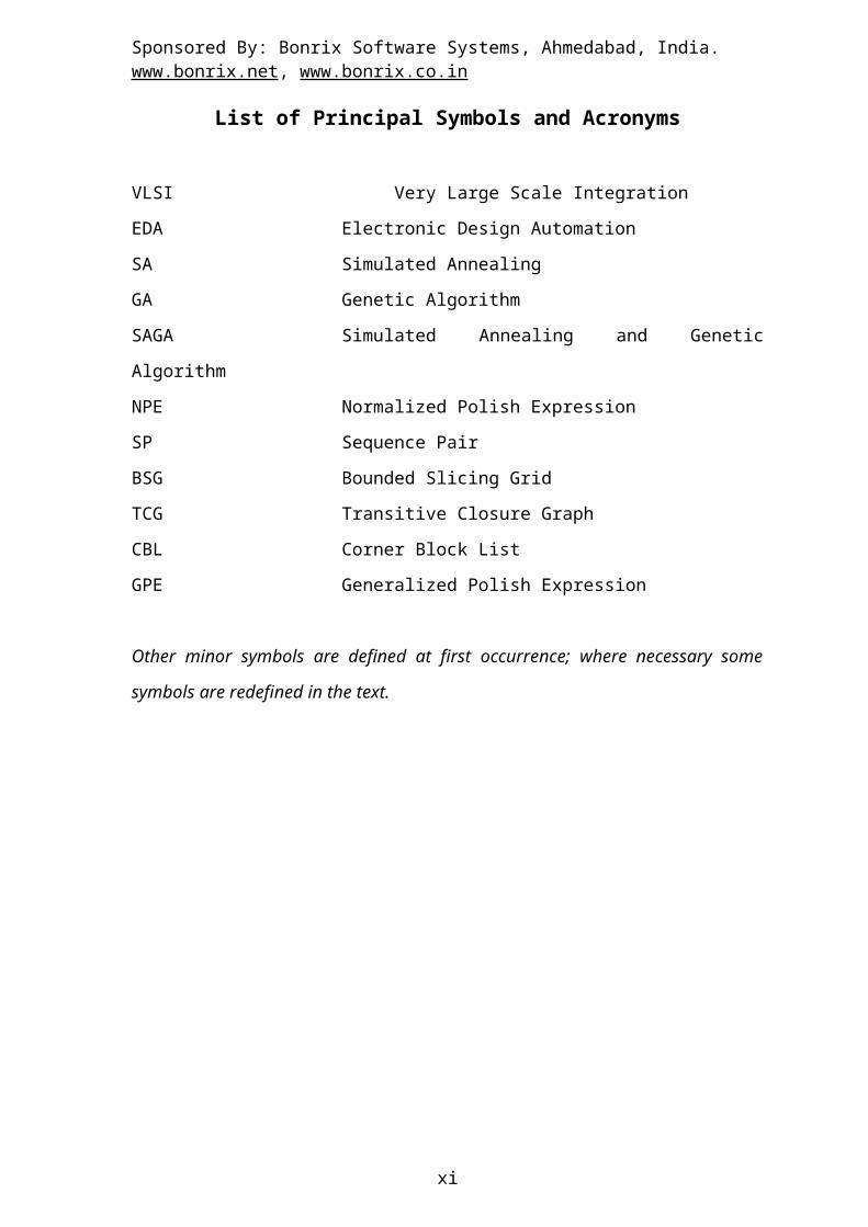


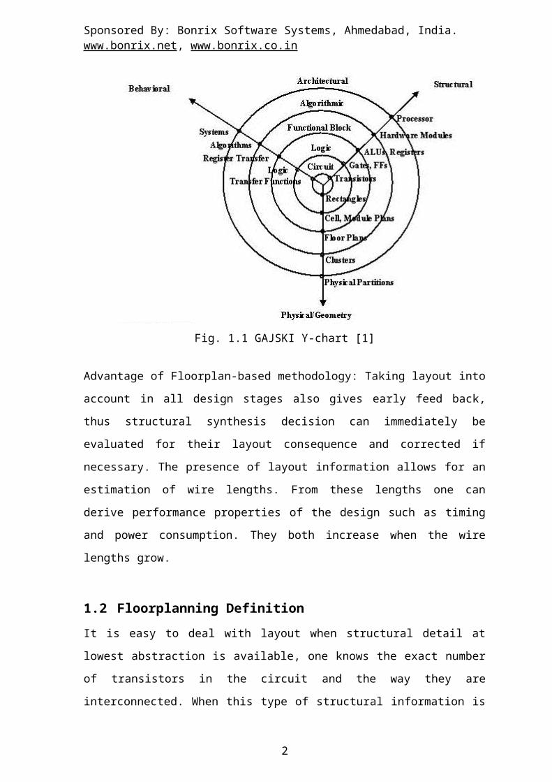
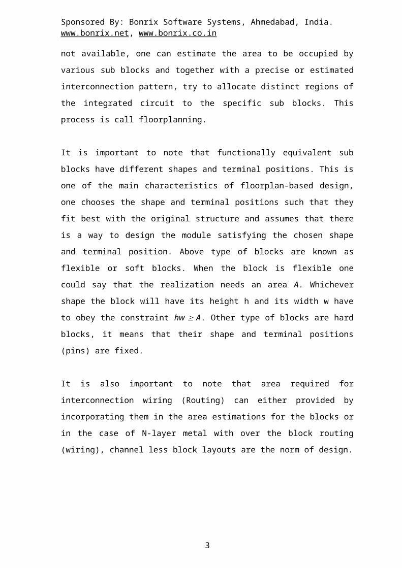
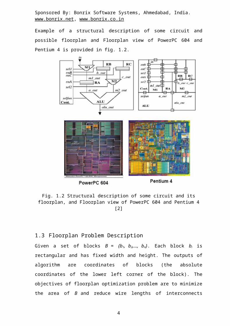
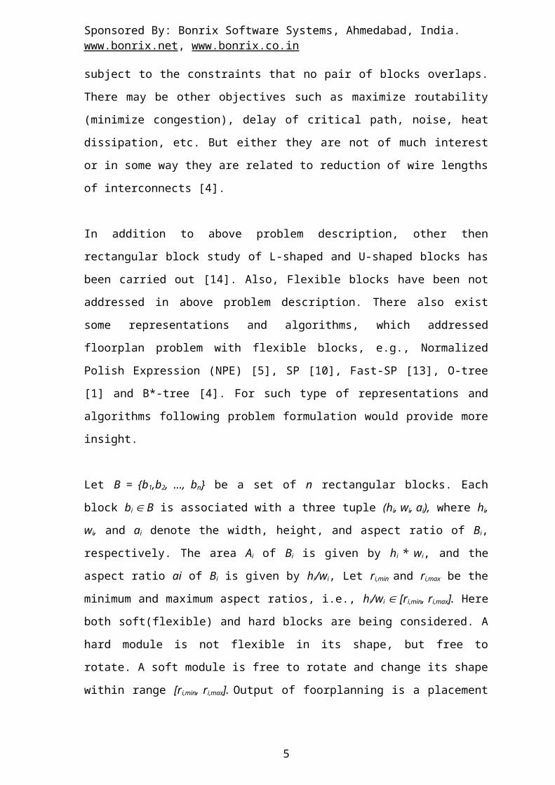
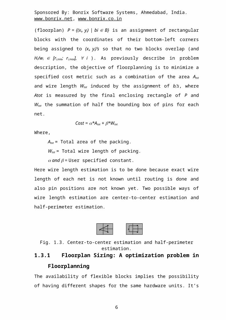

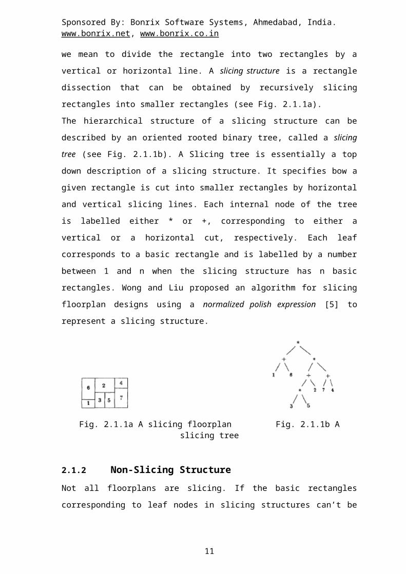
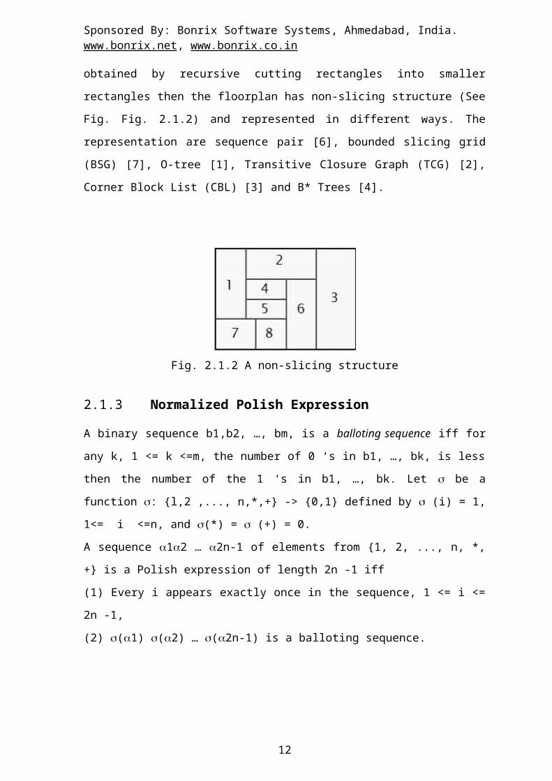
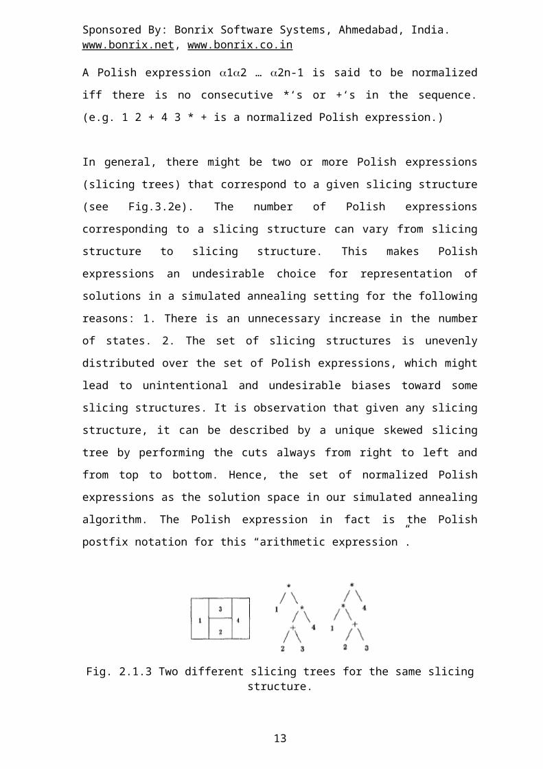
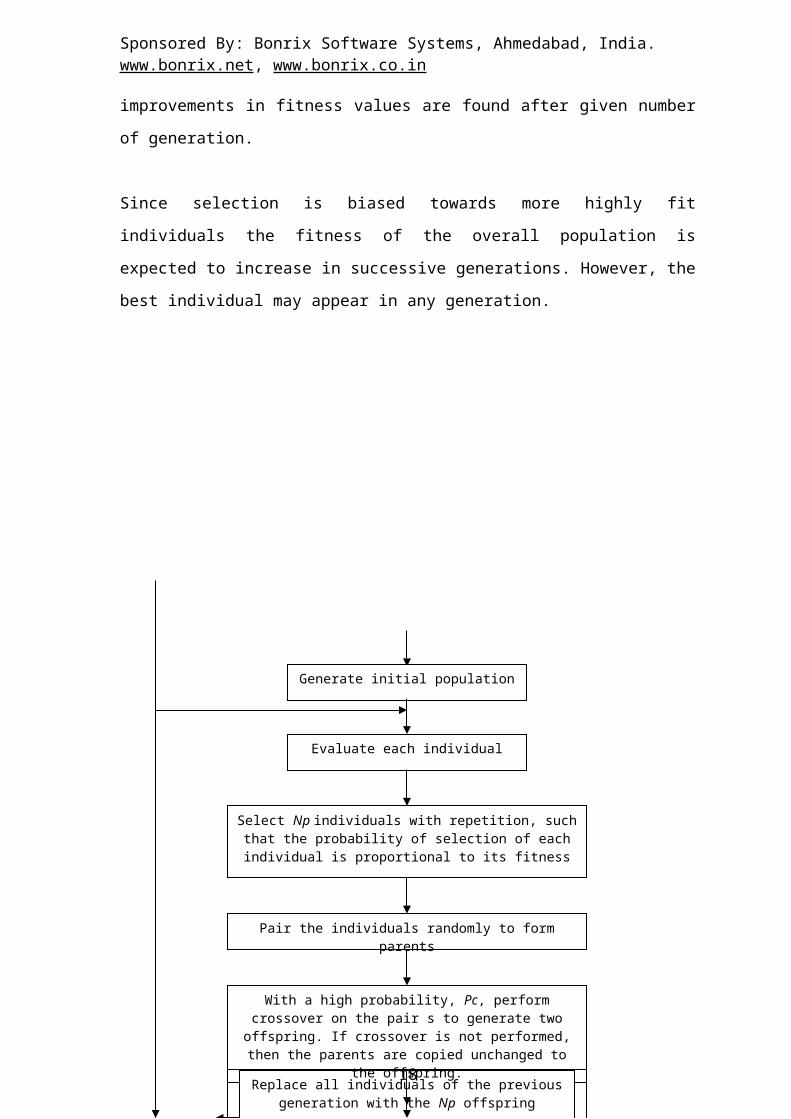
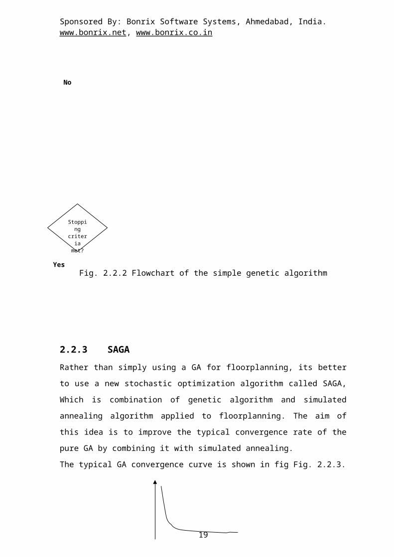
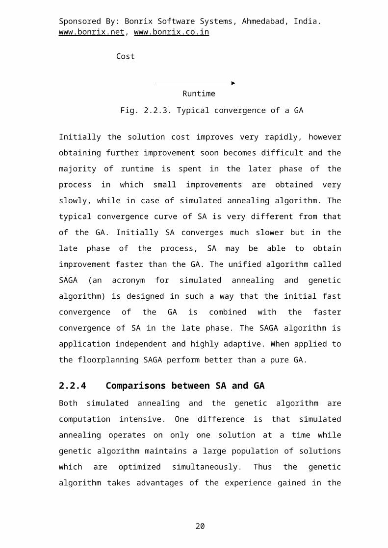
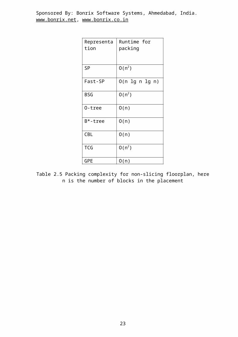
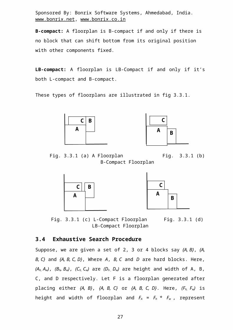
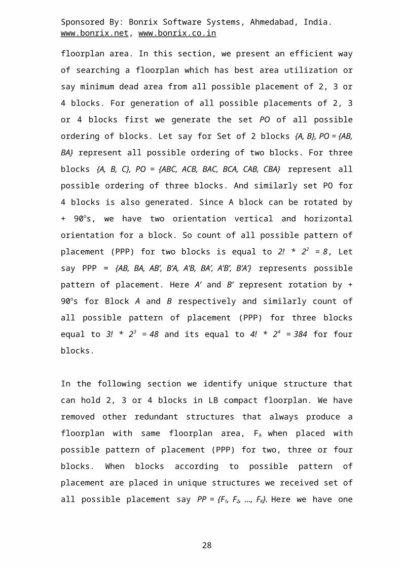
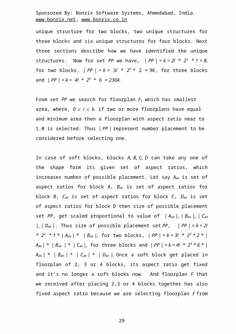
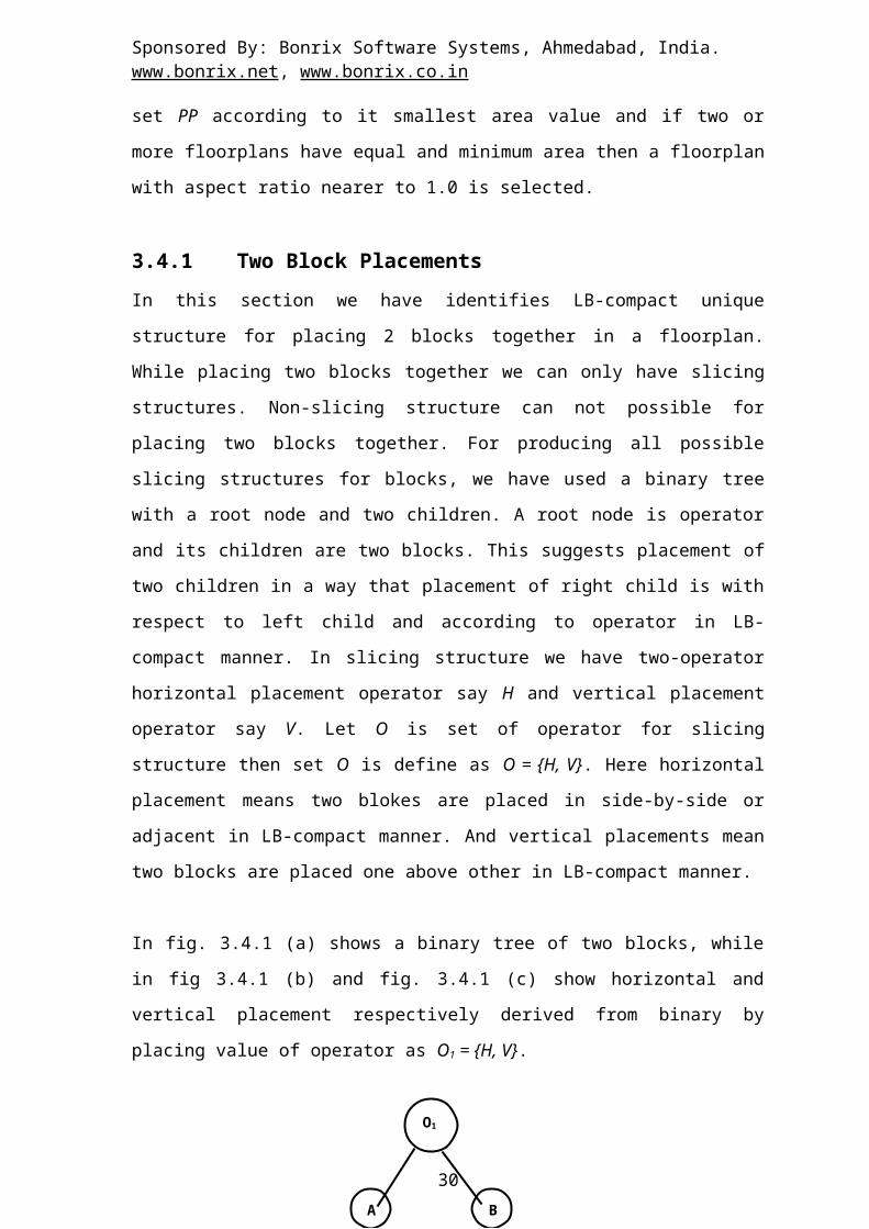
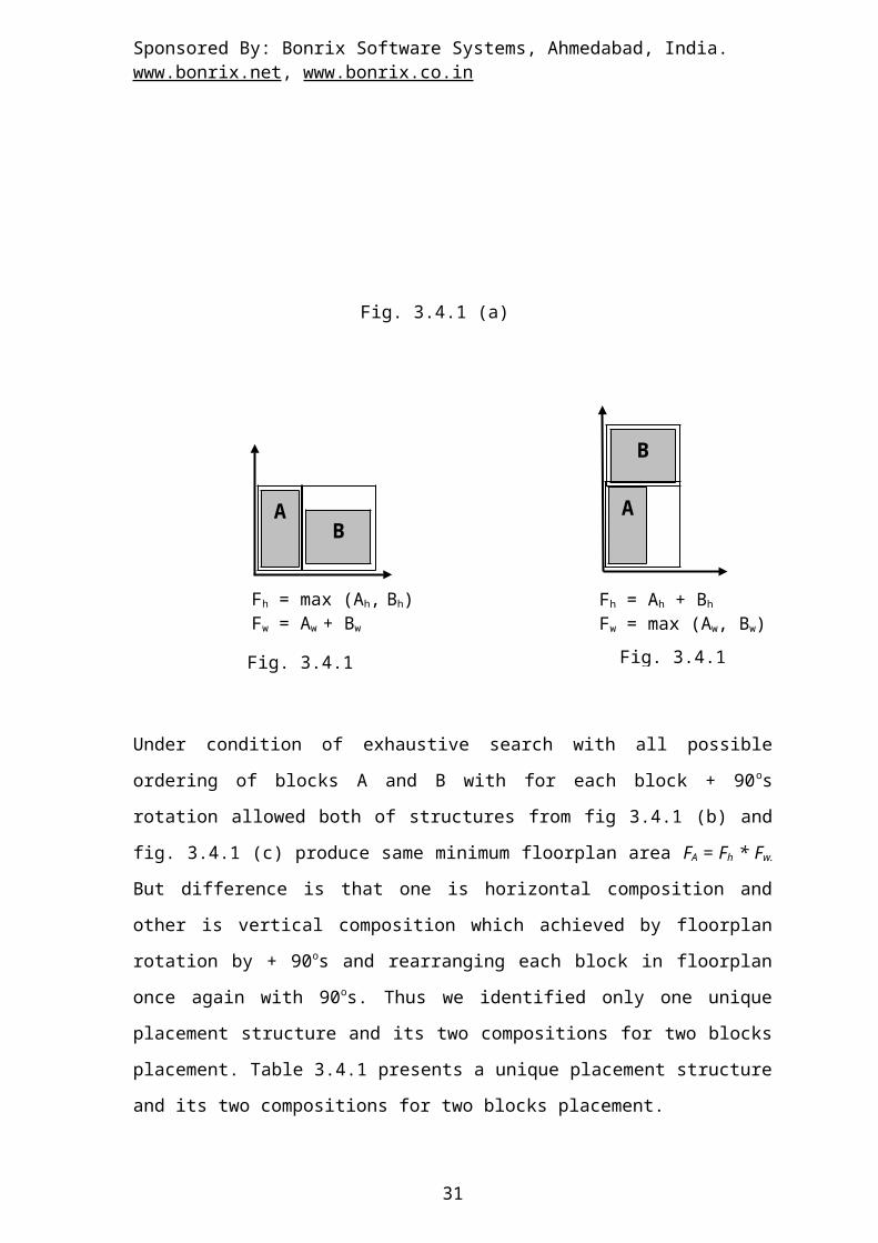
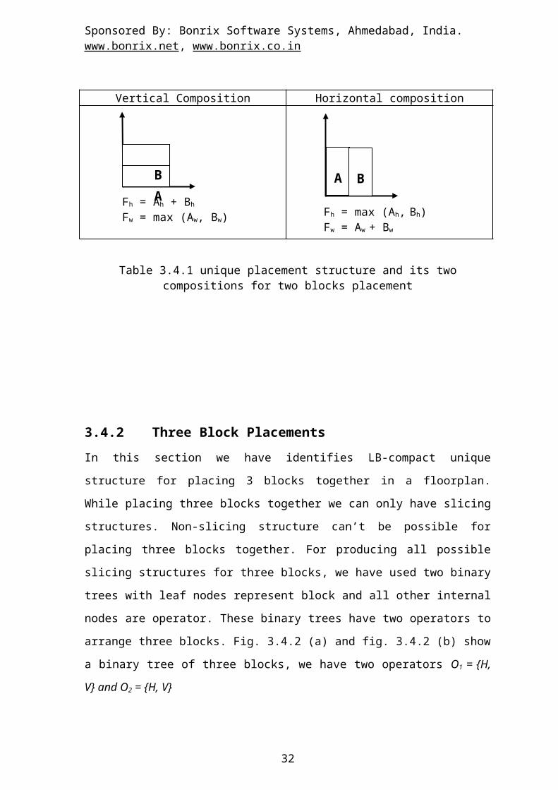
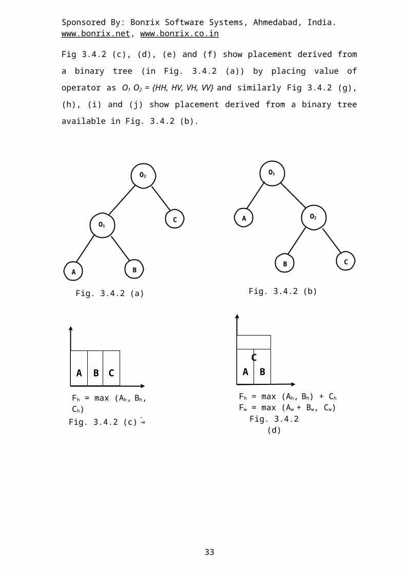
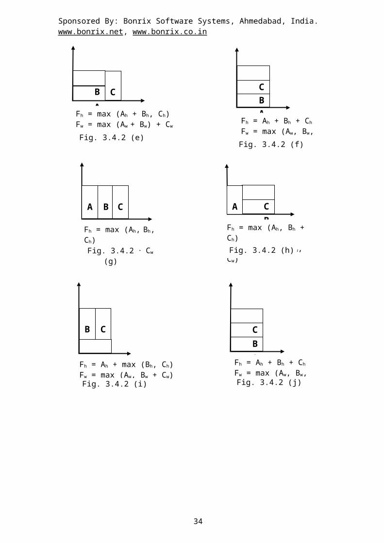
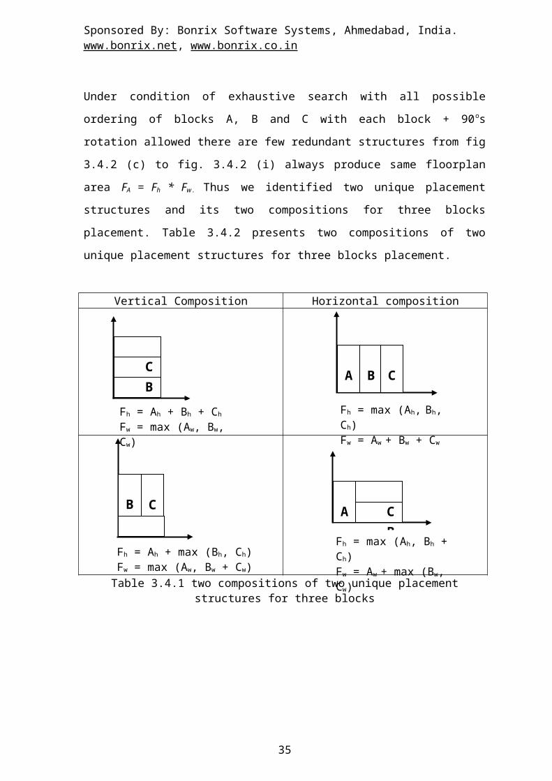
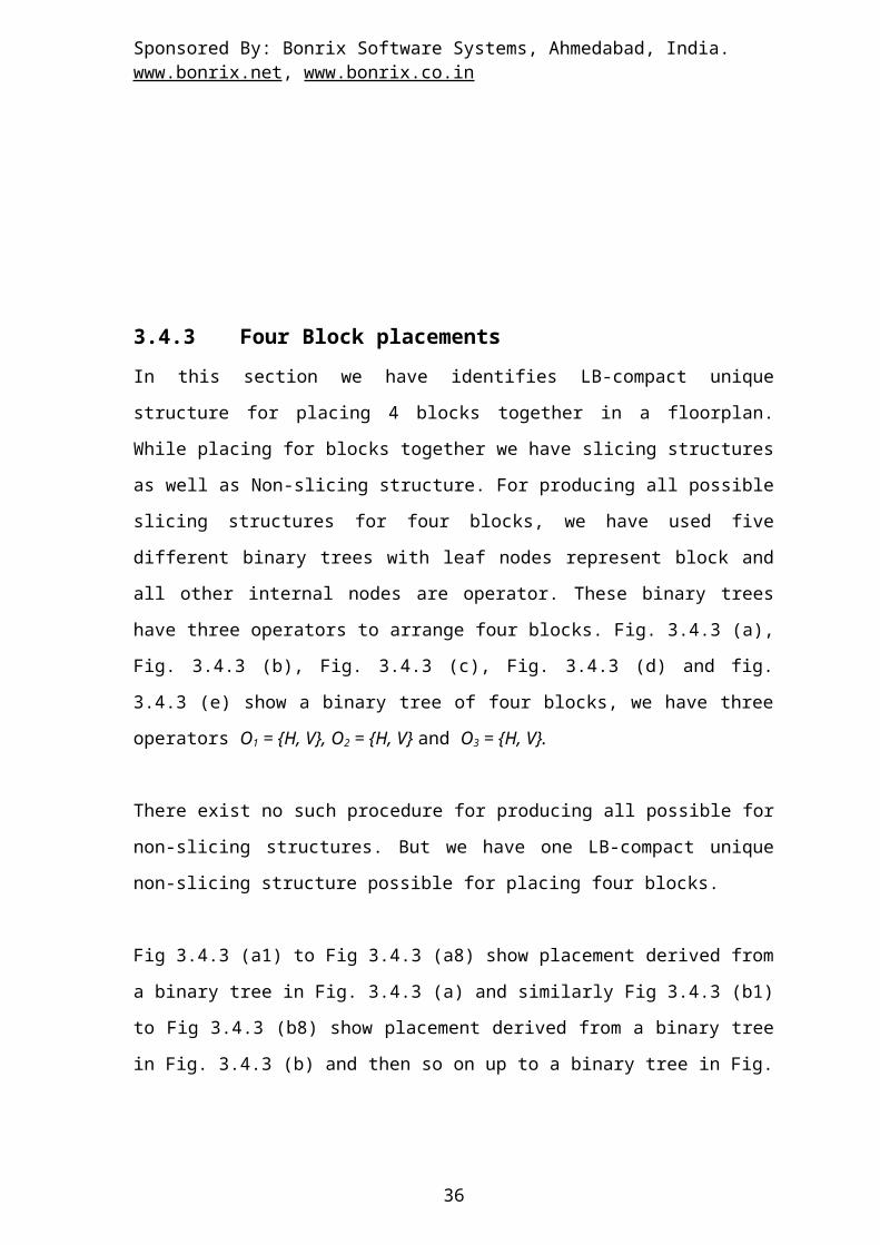
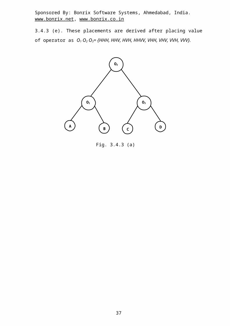
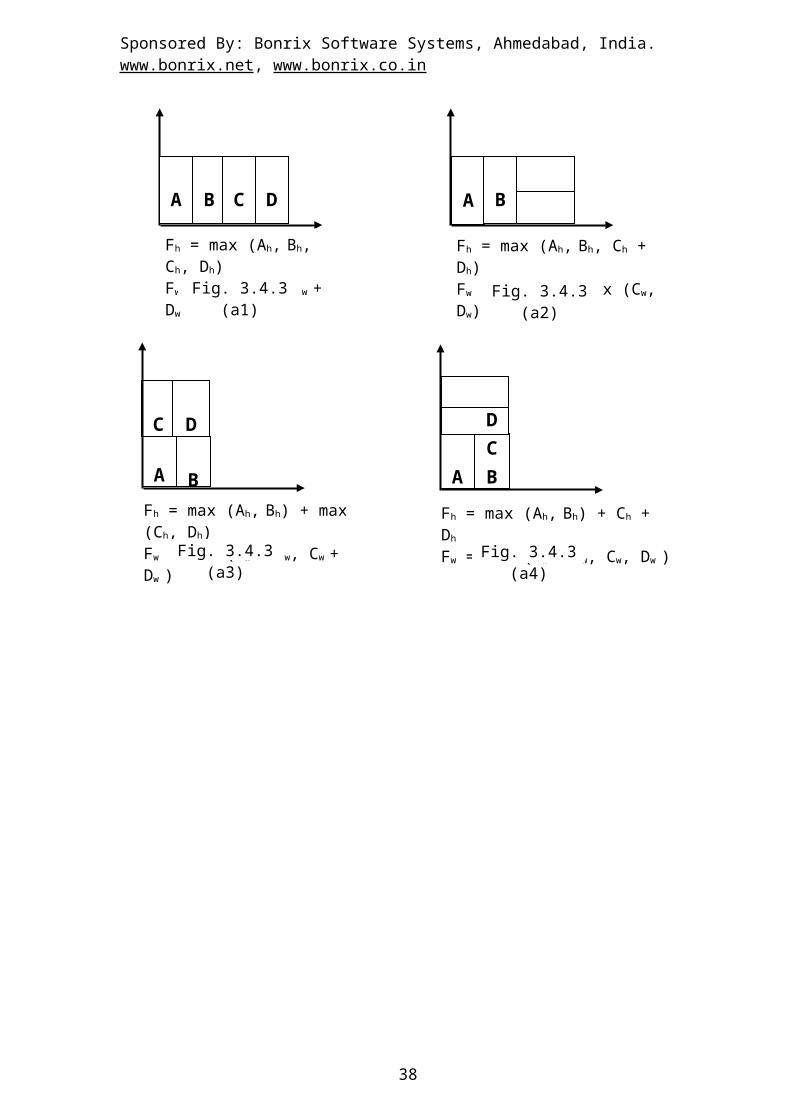
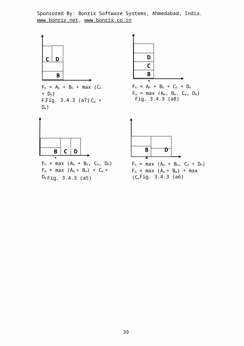
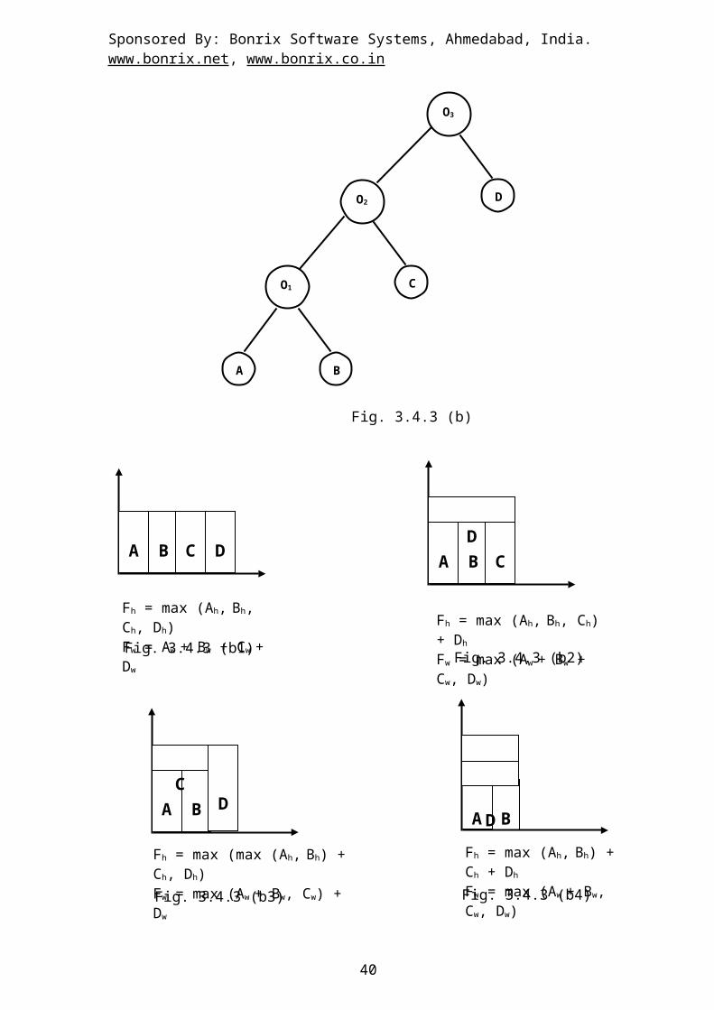
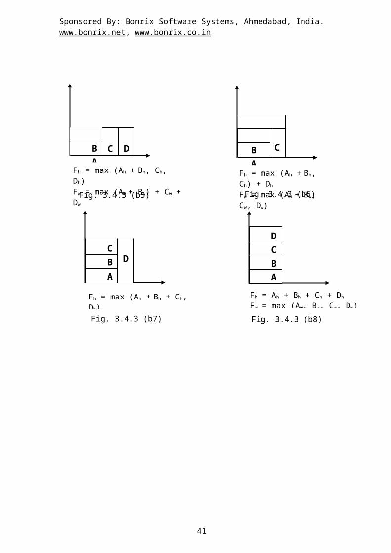
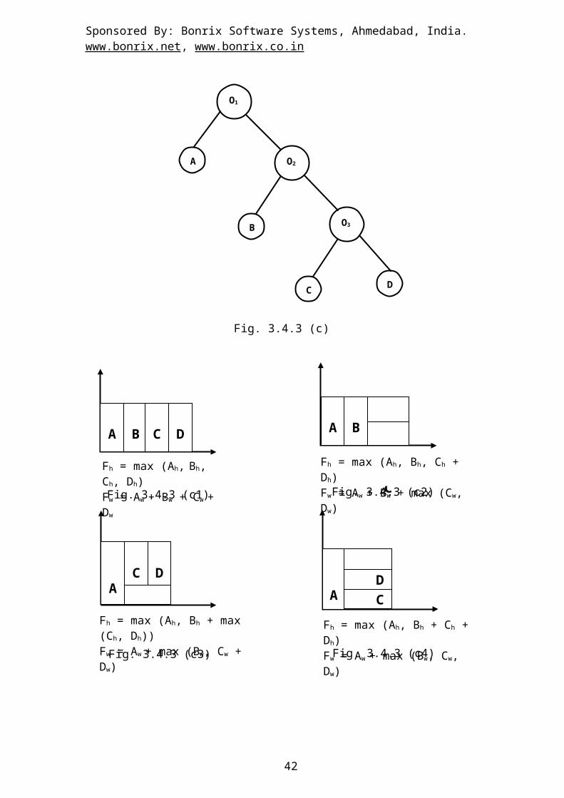
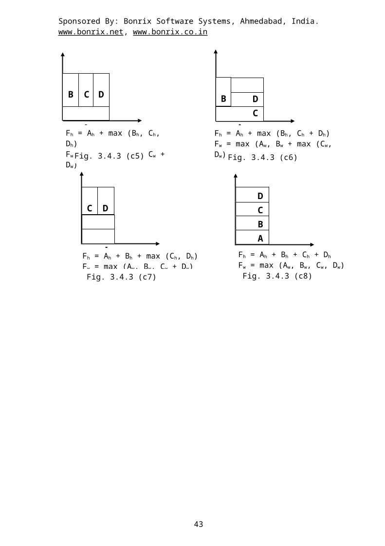
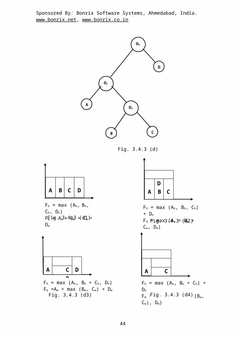
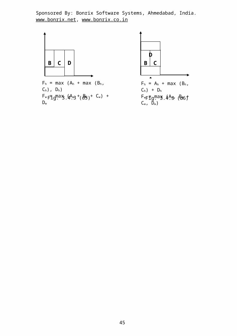
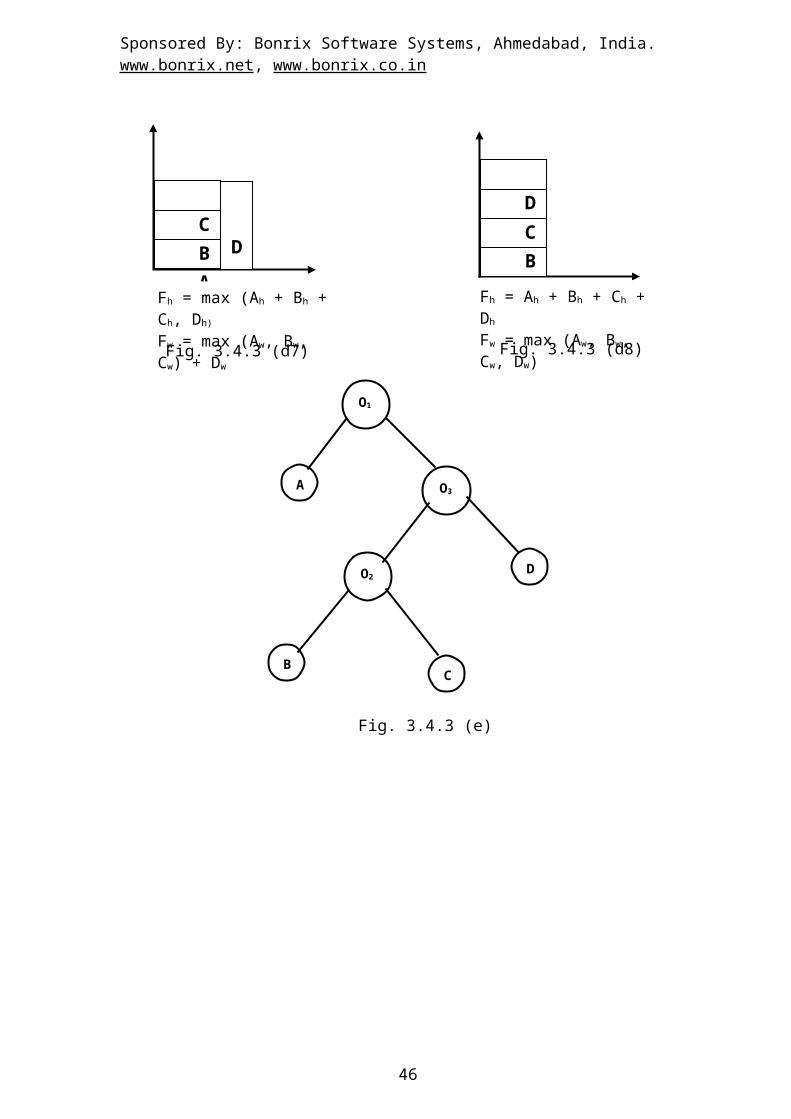
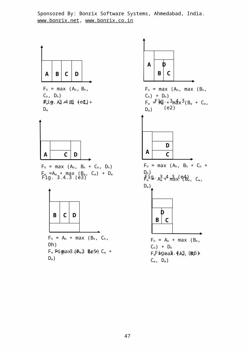
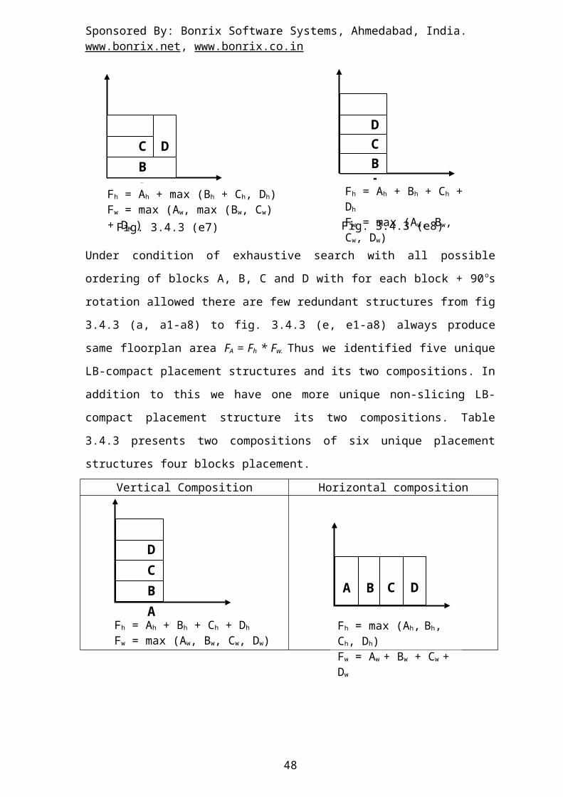
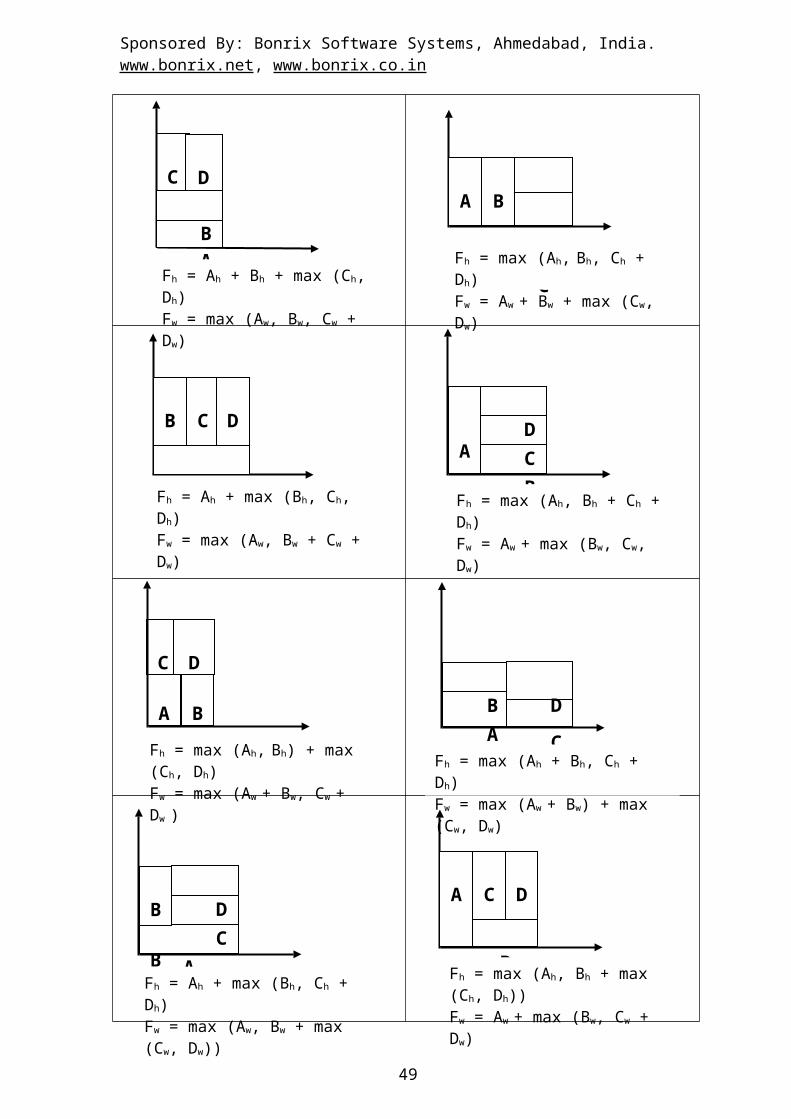
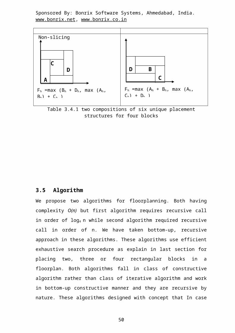
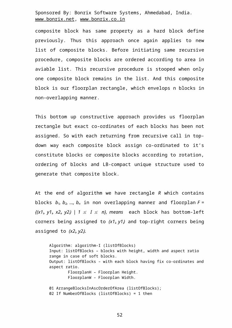
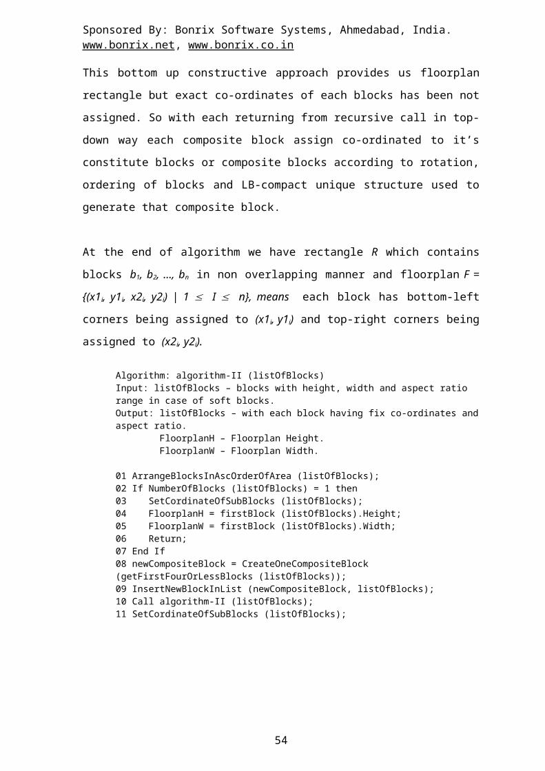
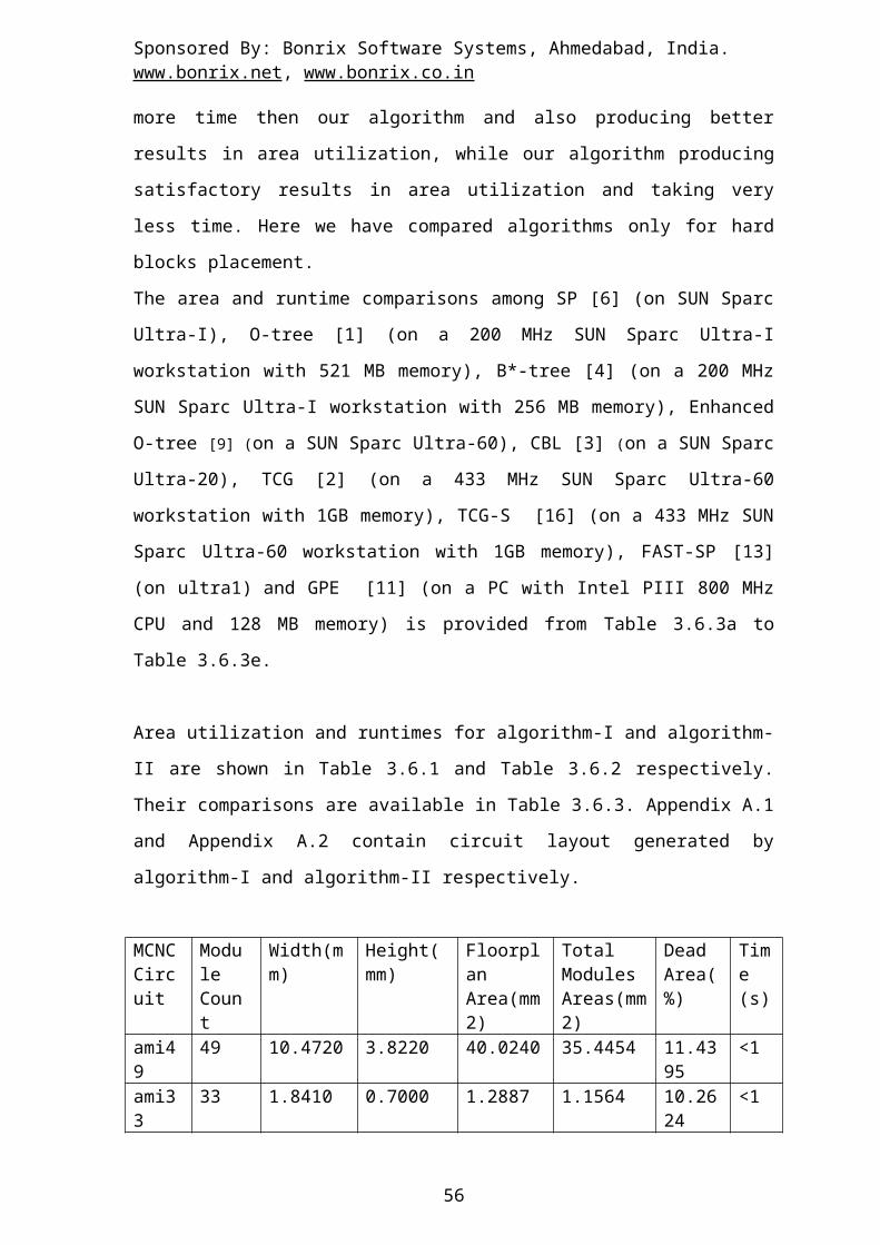
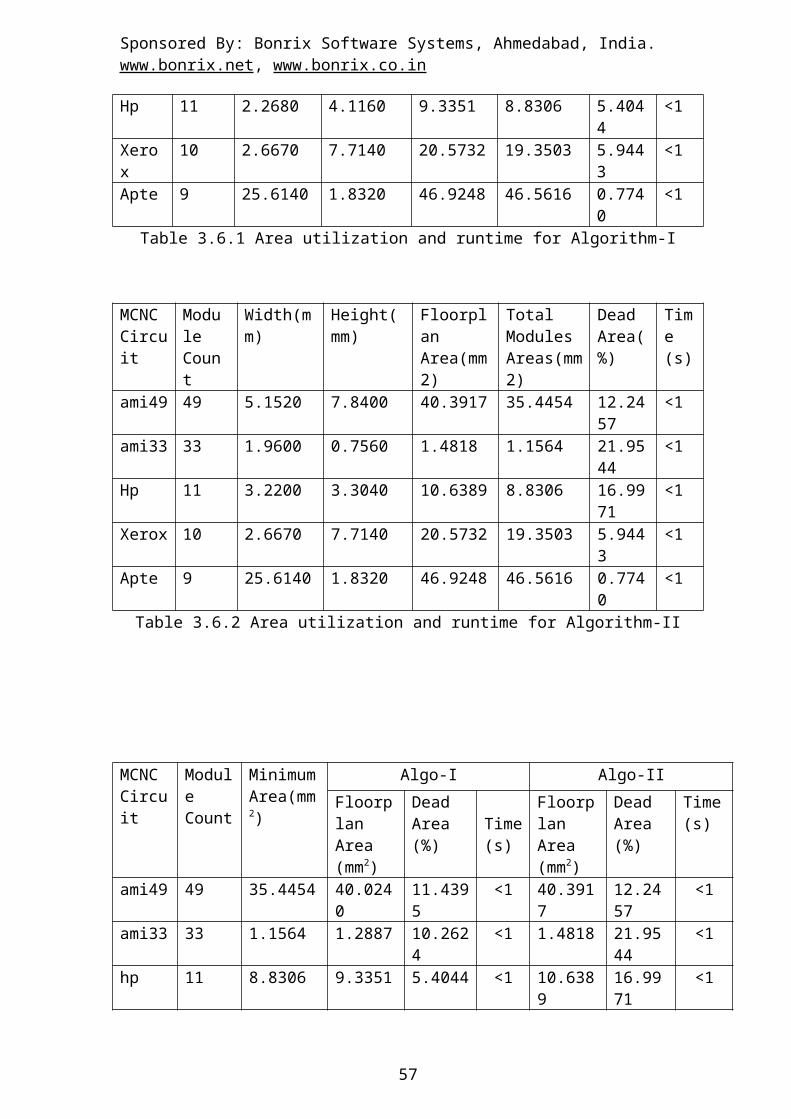
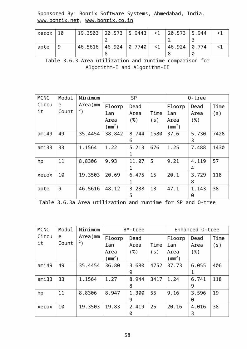
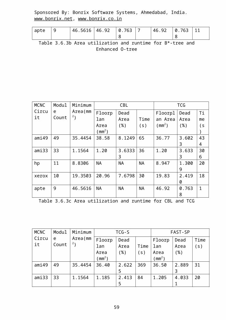
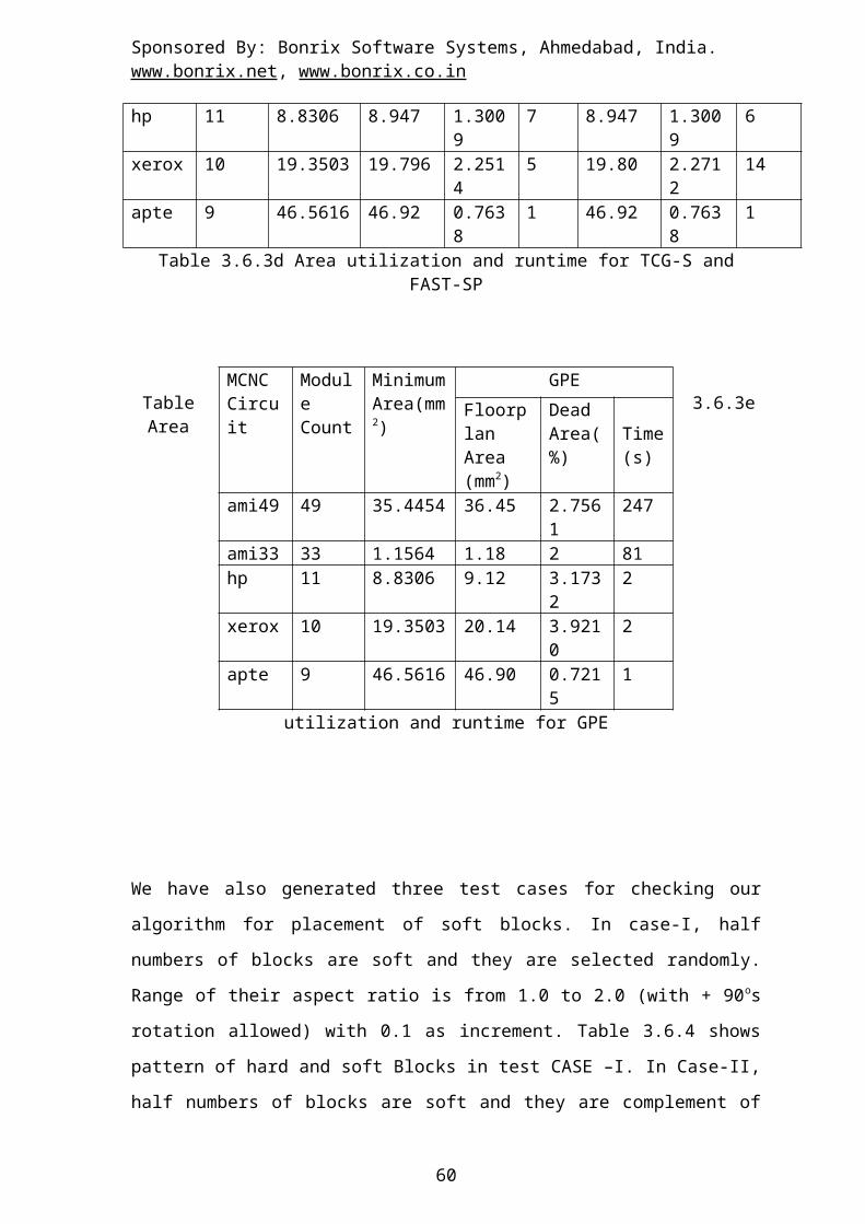
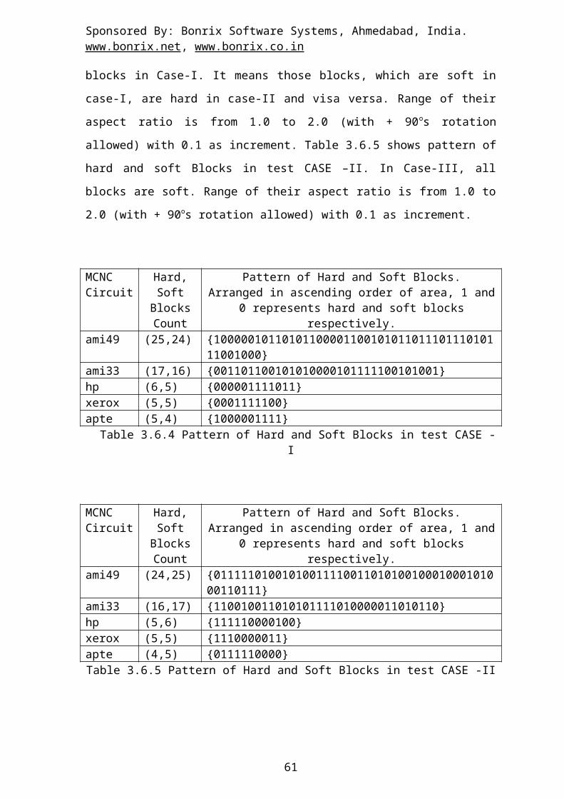
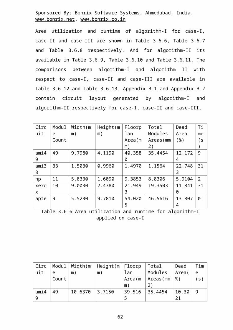
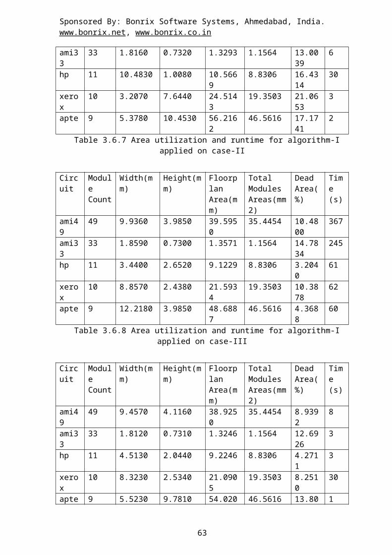
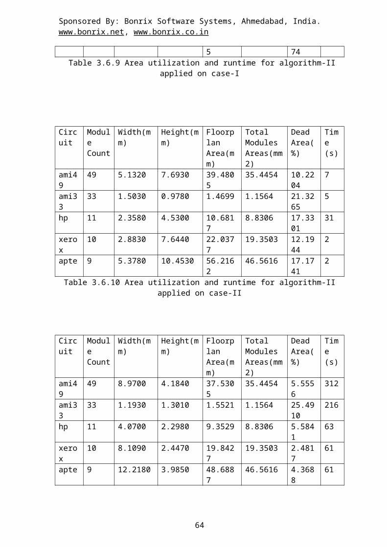
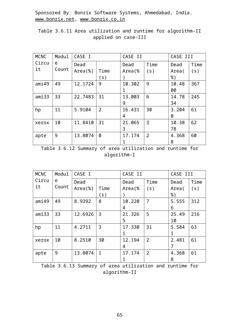

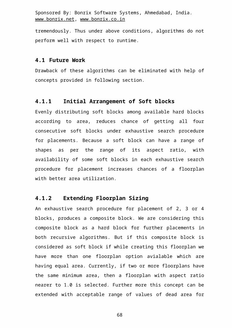
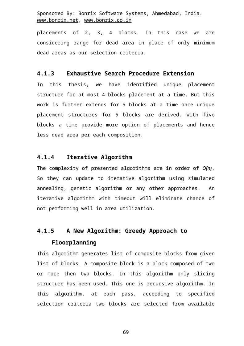
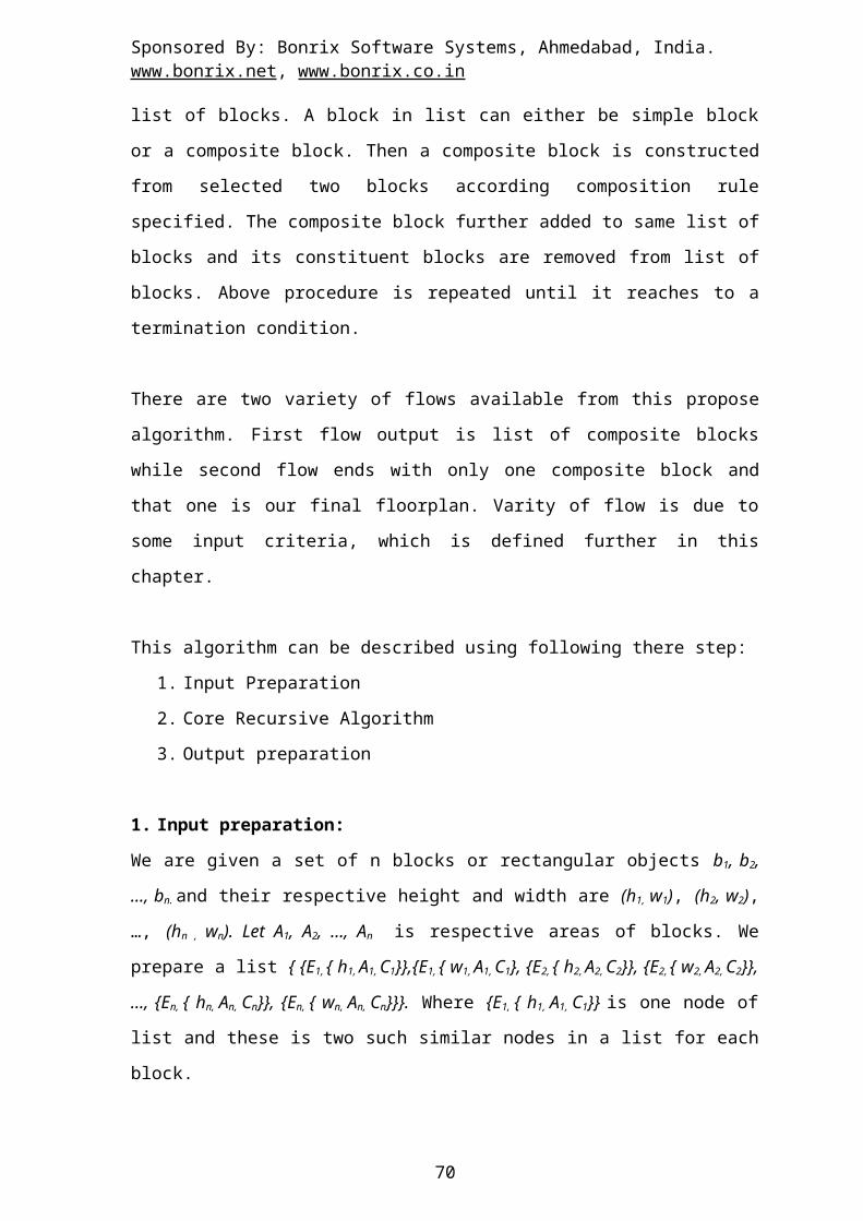


![Floorplanning - National Taiwan Universitycc.ee.ntu.edu.tw/~ywchang/Courses/PD_Source/EDA_floorplanning.pdf · Sherwani 1999]. Basically, simulated annealing-based floorplanning relies](https://static.documents.pub/doc/80x56/5a79a4137f8b9a28678c4078/floorplanning-national-taiwan-ywchangcoursespdsourceedafloorplanningpdfsherwani.jpg)


