Page 1
TÍTULO
Nome completo do Candidato
Subtítulo Building clusters for CRM strategies by
mining airlines customer data
Helena Sofia Guerreiro de Miranda
Project proposal submitted in partial fulfillment of the
requirements for the degree in Mestre em Estatística e
Gestão de Informação
Building clusters for CRM strategies by
mining airlines customer data
Helena Sofia Guerreiro de Miranda
Project Work presented as partial requirement for
obtaining the Master’s degree in Statistics and Information
Management
Page 2
Instituto Superior de Estatística e Gestão de Informação
Universidade Nova de Lisboa
BUILDING CLUSTERS FOR CRM STRATEGIES BY MINING
AIRLINES CUSTOMER DATA
by
Helena Sofia Guerreiro de Miranda
Project Work presented as partial requirement for obtaining the Master’s degree in
Statistics and Information Management, specialization in Marketing Research and CRM
Supervisor: Roberto André Pereira Henriques, Ph. D
November 2012
Page 3
iii
ACKNOWLEDGMENTS
I wish to express my gratitude to my supervisor, Roberto André Pereira
Henriques, Ph. D, who helped me developing this topic. This project work would not be
possible without his help, comments and suggestions.
I also want to thank my family and friends, in particular to my boyfriend, who’s
support was decisive to conclude this work.
Finally, I dedicate this project work to my parents.
Page 4
iv
ABSTRACT
As airlines strive to gain market share and sustain profitability in today’s
economically challenging environment, they should develop new ways to optimize
their frequent flyer programs while increase revenues. Aware of the challenges,
airlines want to implement a customer relationship management (CRM) strategy based
on customer analytics and data mining techniques to support marketing decisions. So,
to achieve this goal, we have to apply clustering techniques to the company customer
databases and develop a single view of customer across their demographic and
behavioral characteristics as well as their value for the company. This will enable the
company to identify the most profitable customers and run marketing campaigns more
efficiently.
KEYWORDS
Cluster analysis, Airlines, Data mining, decision support, customer relationship
management.
Page 5
v
CONTENTS
1. Introduction ................................................................................................................. 1
1.1. Background ........................................................................................................... 1
1.2. Problem ................................................................................................................. 2
1.3. Overall and specific objectives .............................................................................. 2
1.4. Relevance .............................................................................................................. 3
1.5. Methodology ......................................................................................................... 3
1.6. Project Organization ............................................................................................. 4
2. State of art.................................................................................................................... 5
2.1. Introduction .......................................................................................................... 5
2.2. Clustering methods ............................................................................................... 6
2.2.1. k-means .......................................................................................................... 7
2.2.2. SOM ................................................................................................................ 8
2.2.3. Hierarchical SOM ......................................................................................... 11
3. Building Clusters ......................................................................................................... 14
3.1. Dataset used in this project ................................................................................ 14
3.2. Select the variables on which to cluster ............................................................. 15
3.3. Select a distance measure and scale the variables ............................................. 15
3.4. Comparing clustering procedures and deciding the number of clusters ........... 16
3.4.1. k-means ........................................................................................................ 16
3.4.2. SOM EM ....................................................................................................... 18
3.4.3. SOM Toolbox ................................................................................................ 19
3.4.4. HSOM ........................................................................................................... 21
3.5. Interpret and profile clusters .............................................................................. 23
3.5.1. k-means ........................................................................................................ 24
3.5.2. SOM EM ....................................................................................................... 25
3.5.3. SOM Toolbox ................................................................................................ 27
3.5.4. HSOM ........................................................................................................... 29
4. Assess the reliability and validity ............................................................................... 32
5. Conclusion .................................................................................................................. 36
6. Limitations and Further research ............................................................................... 37
7. References .................................................................................................................. 38
Page 6
vi
8. Appendices ................................................................................................................. 41
Page 7
vii
LIST OF FIGURES
Figure 2.1 - Basic k-means algorithm . .............................................................................. 8
Figure 2.2 - Self-Organizing Feature Map ....................................................................... 10
Figure 2.3 - Basic SOM training algorithm ..................................................................... 11
Figure 2.4 - Basic HSOM training Algorithm .................................................................. 13
Figure 3.1 - Cubic Clustering Criterion for Automatic k-means ..................................... 16
Figure 3.2 - k-means distances ...................................................................................... 17
Figure 3.3 - SOM EM distances ....................................................................................... 18
Figure 3.4 - SOM Toolbox U-matrix ............................................................................... 20
Figure 3.5 - SOM Toolbox distances ............................................................................... 21
Figure 3.6 - HSOM 15x10 U-matrix ................................................................................ 22
Figure 3.7 - HSOM distances ........................................................................................... 23
Figure 3.8 - k-means cluster proximities ........................................................................ 25
Figure 3.9 - SOM EM Cluster representation in GeoSOM 15x10 SOM U-matrix............ 27
Figure 3.10 - 4x1 SOM Cluster representation in 15x10 SOM U-matrix......................... 29
Figure 3.11 - HSOM Cluster representation in HSOM U-matrix 15x10 ......................... 31
Figure 4.1 - Distances comparison .................................................................................. 32
Figure 4.2 - k-means results mapped in GeoSOM U-Matrix 15x10 ................................ 33
Figure 4.3 - SOM EM results mapped in GeoSOM U-Matrix 15x10 ................................ 34
Figure 4.4 - HSOM results mapped in GeoSOM U-Matrix 15x10 ................................... 34
Figure 8.1 - Histograms ................................................................................................... 44
Figure 8.2 - Workflow on SAS Guide to choose the Random Sample of 20000 members
and variables correlations ....................................................................................... 47
Figure 8.3 - Workflow on SAS Miner for Automatic k-means to identify outliers ......... 48
Figure 8.4 - Workflow on SAS Miner for Automatic k-means to identify the optima
number of clusters .................................................................................................. 49
Figure 8.5 - Workflow on SAS Miner for SOM to identify the optima number of clusters
................................................................................................................................ 50
Figure 8.6 - SOM 15x10 training parameters in GeoSOM .............................................. 50
Figure 8.7 - SOM 4x1 training parameters in GeoSOM .................................................. 52
Figure 8.8 - SOM 4x1 in a U-matrix 15x10 ...................................................................... 53
Figure 8.9 - SOM 15x10 U-matrix Component Planes .................................................... 54
Figure 8.10 - HSOM training parameters in GeoSOM .................................................... 55
Page 8
viii
Figure 8.11 - HSOM 4x1 in a U-matrix 15x10 ................................................................. 56
Figure 8.12 - Purchase Value and Purchase frequency Component Planes ................... 57
Figure 8.13 - k-means Segment Profile node output ..................................................... 66
Figure 8.14 - SOM Segment Profile node output ........................................................... 67
Figure 8.15 - HSOM training parameters in GeoSOM .................................................... 68
Page 9
ix
LIST OF TABLES
Table 3.1 - Other useful statistics to estimate the number of clusters in the data ....... 17
Table 3.2 - Other useful statistics to estimate the number of clusters in the data ....... 19
Table 3.3 - Other useful statistics to estimate the number of clusters in the data ....... 21
Table 3.4 - Other useful statistics to estimate the number of clusters in the data ....... 23
Table 3.5 - k-means cluster’s size and means ................................................................. 25
Table 3.6 – SOM EM Cluster’s size and means ............................................................... 26
Table 3.7 - SOM Toolbox cluster’s size and means ......................................................... 28
Table 3.8 - HSOM cluster’s size and means .................................................................... 30
Table 4.1 - Coefficient of determination comparison .................................................... 32
Table 4.2 - Pseudo F comparison .................................................................................... 33
Table 4.3 - Inter clusters distances comparison for K=4................................................. 34
Table 8.1 - Variables presented in the database ............................................................ 41
Table 8.2 - Database Simple Statistics for numerical variables ...................................... 42
Table 8.3 - Database missing values sample statistics ................................................... 43
Table 8.4 - Using k-means to identify outliers in the data ............................................. 44
Table 8.5 - Correlation results ........................................................................................ 45
Table 8.6 - k-means means for the variables not used in the clustering task ................ 57
Table 8.7 - SOM EM means for the variables not used in the clustering task ................ 60
Table 8.8 - SOM EM means for the variables not used in the clustering task ................ 62
Table 8.9 - HSOM means for the variables not used in the clustering task ................... 64
Page 10
x
ACRONYMS
Acronyms are presented in alphabetic order.
BCN Barcelona
BR Brazil
BRU Brussels
CH Switzerland
EM Enterprise Miner
ES Spain
EWR New York
FCO Rome
FNC Funchal
FOR Fortaleza
FR France
GB Great Britain
GIG Rio de Janeiro
GRU São Paulo
IT Italy
LAD Luanda
LHR London
LIS Lisbon
MAD Madrid
NL Netherlands
OPO Oporto
ORY Paris
PT Portugal
RW Rest of the World
TER Terceira
US United States
Page 11
1
1. INTRODUCTION
1.1. BACKGROUND
The airlines industry reached a crossroad. The effects of worldwide economic
slump and the rise of the fuel costs have severely impacted airlines economics and
viability. New competitors are actively incentivizing customers to switch brand.
Competition is forcing management to constantly cut costs while raise revenues which
demands for an approach to marketing that is more accountable, efficient and
effective. Thus, to gain and keep market share, companies have to consider customer-
level information (Kumar and Petersen 2005), to target personalized marketing
strategies to their needs and achieve a higher return on investment.
Most companies in the airline industry are facing declining revenue per seat and
increasing competitive pressure because of the deregulation and unfavorable
economic conditions. At the same time, airlines product offering are nearly
indistinguishable from another. Fares came under enormous pressure with pricing
data proliferating on the web. Low costs carriers are opening up new segments,
attracting new customers and taking market share from the establish airlines. Airlines
companies know that competitive advantage in the long run will be based in large part
on solid differentiated customer relationships. Therefore, deliver a consistent and
distinctive customer experience and maintain low operating costs requires customer
databases exploitation. But, how can we analyze more than one million customers and
understand their differences to run campaigns more efficiently? To answer this
challenge we have to use computational techniques such as data mining1. If it is true
that marketing and business users have long used data to segment customers, today’s
volume of customer data imposes more complexity to this task. Therefore,
segmentation, can benefit from the growing sophistication of analytical tools for
dividing customers into more revealing segments which will allow us to group
customers into several homogeneous clusters with similar demographic, behavioral
and value characteristics but collectively different so that we can model different
marketing strategies for each one.
1 As Berry and Linoff define “Data mining is the process of exploration and analysis, by automatic
or semiautomatic means, of large quantities of data in order to discover meaningful patterns and rules.”
Page 12
2
1.2. PROBLEM
Today, there are several algorithms that can be used to segment customers and
sometimes we don’t know which one we should use. Here we intent to evaluate the
performance of three different algorithms, k-means, SOM and Hierarchical SOM and
identify the most efficient for an airline company customer data set.
In addition, we pretend to determine the ideal number of clusters from what
would be a natural solution.
1.3. OVERALL AND SPECIFIC OBJECTIVES
The main objective of this project is to achieve more refined clusters making use
of all the information available and identify the ideal number of segments without any
management restriction. So, to achieve this goal we will use three different clustering
techniques to mine the data and achieve homogenous groups of customers such that
customers in the same cluster are similar in terms of their value, demographic and
behavioral2 characteristics but collectively different. In particular, this project wants to
answer the following questions:
� Which algorithm reveals a better performance segmenting customer
data?
� What would be the ideal number of clusters?
� What are the characteristics of each segment?
� Which is the most and the worst profitable group?
2 In this project we will use behavioral and demographic customer data information to
differentiate by needs.
Page 13
3
1.4. RELEVANCE
This project will produce customer segments that will help to support decision
investments in CRM and define customer service experience to be truly beneficial to
both customer and the airline in two ways:
� by knowing the value of each group of customers the company will be
able to determine the adequate investment in each segment and;
� through the identification of each segment main characteristics the
company will be able to design marketing campaigns with the adequate
incentives and;
Therefore, the company can evolve to a marketing approach that focus on the
different kinds of customers and that is both analytic and value oriented. This means
that it will be possible to make decisions about what marketing programs to initiate
based on customer needs and profitability.
1.5. METHODOLOGY
Given the overall and specific objectives referred before, in section 1.3, the
approach we follow in this project is quantitative. After an in depth study of the
available clustering techniques with special incidence in three algorithms: k-means and
two artificial intelligence methods, SOM and Hierarchical SOM, the project, will focus
on the application of these techniques.
For these purpose, we will use real customer data information of an airline
company3. The database provided includes information on personal characteristics,
client’s transactions and interactions with the company over the last year. To exploit
the data, especially because we are using real data, the application of treatment and
processing techniques is required. These techniques will be presented in section 3.1.
To build the clusters, through the three algorithms referred before, we will use
the SAS software more appropriate for these tasks - SAS Guide version 4.3, SAS Miner
version 9.3 and GeoSOM Suite (Henriques, Bacao et al 2012).
3 The institution in question provided the data in an undertaking of confidentiality on the
information that would otherwise reveal your identity and/or characteristics of its customers.
Page 14
4
Finally, the validation of the results obtained will be based on quality measures
and comparing the results for the three algorithms studied in this project.
1.6. PROJECT ORGANIZATION
This project is organized as follows:
Chapter 2 presents the state of the art related to clustering techniques and focus
on the description, architecture and training process of the k-means, Self-Organizing
Maps and Hierarchical Self-Organizing Map as well as their vantages and limitations.
Chapter 3 presents the application of k-means, SOM and Hierarchical SOM to
build clusters. It will be presented the arguments used in the selection of the variables,
distance measure and scale applied, as well as the determination of the ideal number
of clusters and the interpretation, reliability and validity of the solution achieved for
each algorithm.
Chapter 4 discusses the results achieved for the three clustering techniques
studied in Chapter 3.
Chapter 5 summarizes the conclusions of our research. Open research questions
and future research are also discussed in this chapter.
Page 15
5
2. STATE OF ART
This chapter provides an introduction to cluster analysis. We begin with a high-
level overview of clustering, including a discussion of the various approaches to
dividing objects into sets of clusters and the different types of clusters. We then
describe three specific clustering techniques that represent broad categories of
algorithms and illustrate a variety of concepts: k-means, SOM and Hierarchical SOM.
2.1. INTRODUCTION
Clustering is probably one of the most basic abilities of human kind (Everitt,
Landau et al. 2011). The first step of a learning process is recognition. Once we
identify a “new object” we will try to recognize similarities and differences that could
allow us to classify it. Science also looks for systematic ways to find groups in data
(Kaufman and Rousseeuw 2005). Therefore, whether for understanding or utility,
cluster analysis has long played an important role in a wide variety of fields such as
biology, information retrieval, climate, psychology and medicine, economics,
geosciences, marketing, political science, psychometrics and artificial intelligence
(Kaufman and Rousseeuw 2005; Steinbach, Kumar et al. 2006).
With the objective of identifying meaningful groups that captured the natural
structure of the data, Aristotle, built up an elaborate system for classifying the species
of the animal kingdom in two main groups, those having red blood which are roughly
vertebrates, and those lacking it or invertebrates. In astronomy, Hertzsprung and
Russell classified stars in various categories according their light intensity and their
surface temperature (Kaufman and Rousseeuw 2005). Nowadays, cluster analysis is
used to identify different variations of an illness or condition and cluster analysis can
also be used to detect patterns in the spatial or temporal distribution of a disease or to
optimize the web search results within billions of Web pages (Steinbach, Kumar et al.
2006).
Page 16
6
Despite the utilization of clustering techniques along the time, over the last 30
years, the need of classifying cases in more than three dimensions combined with
major developments in technology and the range of a wealth of algorithms have come
up with the basis of the modern science so-called automatic classification procedures
(Kaufman and Rousseeuw 2005). This so-called automatic classification procedures are
clustering techniques which aim to divide data into groups (clusters) that are
meaningful, useful or both (Steinbach, Kumar et al. 2006) for cluster analysis itself or
as a starting point for other purposes, such as data summarization. Thus, we can
define clustering as the organization of a collection of patterns (usually represented as
a vector of measurements, or point in a multidimensional space) into clusters based on
similarity (Jain, Murty et al. 1999).
Mathematically, we want to group n objects, represented by means of p
attributes, such as age, gender and so on (Kaufman and Rousseeuw 2005). These
measurements can be arranged in an n x p matrix, where the rows correspond to the
objects and the columns to the attributes. Therefore, it should be defined a measure
of similarity4 and calculated the proximity between the n objects to link them
accordingly.
2.2. CLUSTERING METHODS
There are a huge number of algorithms available for clustering. They can be
classified into two main groups: hierarchical and non-hierarchical5
clustering
techniques (Jain and Dubes 1988). Here, we will approach non-hierarchical methods
due to the advantages in applications in large data sets for which the hierarchical
methods and the construction of a dendogram is computationally prohibitive (Jain,
4 Later in this chapter, we will describe the most widely used measures of similarity.
5 Non-hierarchical clustering or partitional clustering is simply a division set of data objects into
non-overlapping subsets (clusters) such that each data object is in exactly one subset. If we allow
clusters to have subclusters, then we obtain a hierarchical clustering, which is a set of nested clusters
that are organized as a tree.
Page 17
7
Murty et al. 1999)6. Even though there are several methods that can be classified as
non-hierarchical clustering, we will cover k-means, Self-Organizing Map and
Hierarchical SOM. Each of these three methods were chosen for one reason: k-means
is one of the most widely used techniques for clustering analysis (Jain, Murty et al.
1999), SOM has been pointed out to be less prone to local optima than k-means which
allows the search space to be better explored and guarantees better results (Bodt,
Cottrell et al. 1999; Bacao, Lobo et al. 2005) and, HSOM is a tentative to achieve even
better results.
2.2.1. k-means
The k-means may be one of the oldest and most widely used clustering
algorithms among data miners (Steinbach, Kumar et al. 2006). The k-means algorithm
is popular because it is easy to implement and has linear time complexity in the size of
the data set besides that it has capacity to handle with large databases (Jain, Murty et
al. 1999). This algorithm uses an iterative procedure, to set cluster centers which are
commonly called seeds or centroids. These centroids are the vectors of mean7
characteristics across the clusters members.
So, given the n points that become the initial cluster centers, each of the
remaining points is assigned to the closest k cluster center according to its Euclidean
distance. Once all points are grouped into k clusters, new clusters centers are
calculated. This interactive process will stop when no more reassignments occur or the
squared error ceases to decrease significantly.
This algorithm tend to produce equal-sized clusters because it implicitly assumes
spherical shaped clusters a common error variance (Everitt, Landau et al. 2011) and is
6 Kaufman and Rousseeuw 2005, point out that hierarchical techniques do not really compete
with non-hierarchical methods because they do not really pursue the same goal, as they try to describe
the data in a totally different way. Indeed a partitioning method tries to select the best clustering with k
groups, which is not the goal of hierarchical methods because hierarchical methods can never repair
what was done in the previous steps.
7 Note that k-means is only defined over numeric continuous valued data since the ability to
compute the mean is required.
Page 18
8
not suitable for discovering clusters with convex shapes or very different sizes (Han
and Kamber 2006). Due to the use of Euclidean distance, k-means is especially
effective dealing with normal (or Gaussian) distributions. k-means is formally described
in Figure 2.1.
Figure 2.1 - Basic k-means algorithm (Source: Steinbach and Kumar 2006).
According to Jain, Murty and Flynn (1999) a major problem with this algorithm is
that it is sensitive to the selection of the initial partition and may converge to a local
minimum of the criterion function value if the initial partition is not properly chosen.
Also, k-means method can only be applied when the means of clusters are defined and
do not perform well with qualitative attributes. This algorithm is very sensitive to noise
and outlier data (Han and Kamber 2006).
2.2.2. SOM
Self-Organizing Map (SOM) is a type of artificial neural network model (ANN) that
have been used extensively over the past three decades for both classification and
clustering (Jain and Mao 1996). Artificial neural networks are one of the most powerful
tools in data mining. ANNs “learn” and generalize from external inputs, mimicking the
structure of neurons that constitute the human brain to discover unknown patterns
and relationships in the data (Hertz, Krogh et al. 1991). For this reason, neuronal
networks can provide great flexibility in handling with non-linearity and variable-
interactions that can be important in clustering modeling applications.
SOM was first proposed by Tuevo Kohonen in 1982 (Kohonen 1982) and was
originally used for image and sound but also to clustering individuals. SOM basic idea is
Basic K-Means algorithm
1: Select k points as initial centroids.
2: repeat.
3: Form k clusters by assigning each point to its closest centroid.
4: Recompute the centroid of each cluster.
5: until Centroids do not change.
Page 19
9
to map high-dimensional data onto one, two or three dimensions8, maintaining the
topological relations between data patterns. SOM “extract and illustrate” the essential
structures in a dataset, through a map resulting from an unsupervised learning process
(Kaski and Kohonen 1996; Kaski, Nikkilä et al. 1998). SOM involve iterative procedures
for associating a finite number of inputs (object vectors) with a finite number of
representational points in such a way that proximity relationships between the inputs
are respected by these representational points. The algorithm performs a non linear
mapping from a high dimensional data space to a low dimensional space, typically two-
dimensional, rectangular grid9 (Kohonen 2001) which allows the presentation of a
multidimensional data in two dimensions. To do this, SOM uses an input layer and an
output layer. Each unit in the output layer10
is connected to units (or attributes11
) in
the input layer and the strength of this connection is measured by a weight. The
weights between the input and the output layer are iteratively changed (this is called
learning) until a termination criterion is satisfied. Further, SOM’s convergence is
controlled by various parameters such as the learning rate and a neighborhood of the
winning layer input node in which learning takes place. Due to this competitive
learning, similar patterns are automatically grouped by a single unit (neuron) based on
data correlation. The output is said stable if no pattern in the training data changes its
category after a finite number of learning interactions. To reach stability, the learning
rate should be decreased to zero as iterations progress and this affects the plasticity,
which is the ability of the algorithm to adapt to new data (Jain, Murty et al. 1999).
8 Although higher dimensional grids are possible, they are not generally used since their
visualization is much more problematic. 9 The lattice type may have several forms like rectangular, hexagonal or even irregular.
10 The number of units in the output layer is specified by the user according to the size and shape
of the topological map. 11
The number of units represents the number of attributes on which customers are being
characterized.
Page 20
(Source: http://www.lohninger.com/helpcsuite/kohonen_network_
Mathematically, this implies to calculate the distance for any point x in the input
space to determine the closest neural unit j* which is also called the Best Matching
Unit (BMU) for x. The neuron with the best matching will be
given learning rate α and defined neighborhood function
usually a decreasing function that starts with a relative large value
corresponding to the ordering phase and ends with a small v
fine adjustment phase. The neighborhood function,
the neurons that will be activated and whose positions will be modified. This function
converges to zero as the number of iterations tend to infin
end when a predetermined number of epochs is reached. Therefore, if each neuron is
taken to represent one cluster, the clusters will have a convex polyhedral shape as we
have with the algorithm
defined as follows.
Figure 2.2 - Self-Organizing Feature Map
http://www.lohninger.com/helpcsuite/kohonen_network_
background_information.htm)
Mathematically, this implies to calculate the distance for any point x in the input
space to determine the closest neural unit j* which is also called the Best Matching
Unit (BMU) for x. The neuron with the best matching will be update according to a
given learning rate α and defined neighborhood function . The learning rate is
usually a decreasing function that starts with a relative large value
corresponding to the ordering phase and ends with a small value, corresponding to the
fine adjustment phase. The neighborhood function, on the other hand, aim to define
the neurons that will be activated and whose positions will be modified. This function
converges to zero as the number of iterations tend to infinitive. The training process
end when a predetermined number of epochs is reached. Therefore, if each neuron is
taken to represent one cluster, the clusters will have a convex polyhedral shape as we
have with the algorithm k-means (Lampinen and Oja 1992). Algebraically, this can be
10
http://www.lohninger.com/helpcsuite/kohonen_network_-
Mathematically, this implies to calculate the distance for any point x in the input
space to determine the closest neural unit j* which is also called the Best Matching
update according to a
. The learning rate is
usually a decreasing function that starts with a relative large value in the beginning,
alue, corresponding to the
the other hand, aim to define
the neurons that will be activated and whose positions will be modified. This function
itive. The training process
end when a predetermined number of epochs is reached. Therefore, if each neuron is
taken to represent one cluster, the clusters will have a convex polyhedral shape as we
. Algebraically, this can be
Page 21
11
Figure 2.3 - Basic SOM training algorithm (Source: Adapted from Huang, Tzeng et al 2007 and
Bacao, Lobo et al 2005)
One of the interesting properties of SOM is the capability of detecting small
differences between the objects and its efficiency in finding multivariate data outliers
(Munoz and Muruzabal 1998; Nag, Mitra et al. 2005). Nevertheless, SOM as k-means,
may generate a suboptimal partition if the initial weights are not chosen properly.
Depending on the initial parameterization, the SOM can produce different results. In
fact, there are multiple choices that have significant consequences on the final result,
such as: the size of the map, the output space dimension, the initialization and the
neighborhood function.
2.2.3. Hierarchical SOM
As we have already referred, the airline’s customer information increases every
day, placing additional pressure on the existing analysis tools and addressing concerns
of efficiency, high-dimensionality feature extraction and data projection (Mao and Jain
1995).Therefore, clustering may benefit from HSOM multilayer structure to gain
efficiency throughout the stratification and exploitation of the databases from
different thematic perspectives.
Basic SOM training algorithm
1: Set at random the initial synaptic weights between ]0,1[.
2: Calculate the winner-takes all neuron j * at iteraction p using the criterion:
where �.� denotes the Euclidean distance, and m denotes the number of neurons in the output layer.
3: Update all neuron's weights using the folling equation:
4: Decrease the value of the learning rate and the radius of the neighborhood function
5: until the learning rate, assuming values in ]0,1[, initialized to a given initial learning rate reaches 0.
where α denotes the learning rate and Λj (p ) is the neighbourhood function centered around the
winner-takes all neuron j * at iteraction p .
Page 22
12
Traditional clustering methods, in which self-organizing maps (Kohonen 2001)
are included, are very sensitive to divergent variables12
, to avoid this problem we
propose the use of a hierarchical structure to explore and cluster customer
information. With HSOM, variables are grouped in topics, where each topic will be
independently clustered. These partial clusters are then used to create a global
partition. By performing the clustering task in two stages, based on individual topics
and only then globally, HSOM is less sensitive to divergent variables then SOM and
other traditional clustering methods because divergent variables will merely have a
direct impact on their own topic. In fact, this approach ensembles two main
advantages: it reduces the dimensionality of the inputs and the number of units in
each SOM granting HSOM less computational effort than a standard SOM
(Mukkulainen 1990) and allow HSOM to fit better due to it’s a hierarchical structure,
less sensitive to outliers and which may also provide an easier interpretation of the
results.
Hierarchical SOM structure looks like a multilayer perceptron neural network,
however, HSOM have different algorithms and types of interaction between layers.
When the type of interaction between SOMs is of train/map type we have a strict
subordination between SOMs, because it uses the outputs of one SOM to feed the
other SOM, asking the second SOM to map the original data patterns using the outputs
of the first one (Luttrell 1989).
In HSOM, the first level of SOM filters which data patterns are sent to the second
level SOM by moving forward13
the index of the best matching unit, the quantization
error, the coordinates of the best matching unit and all activation values for all units of
the first level or any other type of data (Henriques 2010). This information which is
passed to the second level SOM is used to train it. A specific output of one SOM Layer
could be the original or an empty data pattern. However, many different arrangements
are feasible for Hierarchical SOMs. These arrangements can vary in the number of
12
Divergent variables are those that present significant differences to the general tendency. 13
Only the data patterns with the highest variance will pass to the second level.
Page 23
13
layers used, the different methods connections are made and also in the information
which is sent through each connection.
There are different possible taxonomies for Hierarchical SOMs. They can be
classified as agglomerative or divisive (Ding and He 2002). The level of data abstraction
in the agglomerative HSOM increases as the hierarchy goes up and the main goal is to
create clusters which will be more general and provide an easier way to understand
the data. Divisive HSOM is mostly less precise in the first level and is likely to be more
exact as the levels of HSOM (Henriques 2010) go up. In the second level, the
agglomerative HSOMs can be arranged by specific subjects about the clusters whilst
divisive HSOMs can be arranged into static or dynamic. Here, we will focus on thematic
agglomerative hierarchical SOM, and refer to it simply as HSOM.
Figure 2.4 - Basic HSOM training Algorithm (Source: Henriques, R. 2010)
The main advantage of HSOM or SOM clustering algorithm with respect to k-
means is the adaptive distance measure. In the k-means large clusters can be split into
smaller ones and small clusters can be are merged together, until all the clusters are of
desired size (Ding and He 2002).
Basic HSOM training algorithm
Let
X be the set of n training patterns
be a vector with m components
t be a theme composed by components of from
be a thematic SOM map relative to the theme t , i.e. a SOM trained with the components of belonging
to the theme t .
be the image of in the maps , i.e. the concatenation of the outputs of all maps when pattern is
presented
O be the set of all . This set constitutes the modified training set for the top level SOM.
Do
1: For each theme t
2: Train each thematic SOM map in a standard way using as input the relevant components of X .
3: Create the set of modified training patterns O as a concatenation of the possible outputs of maps ,
using for each input pattern:
a. The coordinates of its BMU.
b. Its quantization error.
c. Its distance to each unit (i.e. , all quantization errors).
4: Train the top level SOM using as input the set of modified training patterns O .
Page 24
14
3. BUILDING CLUSTERS
3.1. DATASET USED IN THIS PROJECT
In this project, we use an airline customer database to evaluate the performance
of k-means, SOM and H-SOM. This dataset is a random sample of flight active14
member’s original database. This data contains information of 20.000 customers and
describes customer’s age, gender, country of residence, number of years has a client,
top routes, top brand booking, the number of months since last flight, as well as
member’s flight miles, promotion miles and redeemed miles, and the number of flown
segments. Table 8.1 describes the variables presented in the database.
The data has been validated according to the airlines business criteria; gender
must be male or female, age should vary between 2 and 112 years, the country code
can be classified as Portugal, Brazil, France, Great Britain, Italy, U.S, Switzerland, Spain,
Netherlands or Rest of the World. The number of years since enrollment should vary
between 0 and 20. Having flight miles implies to have flown segments, such as having
promotion miles means that the client has bought during a promotion and having
redeemed miles requires swap flight miles for free flight coupons. Further, according
to Table 8.3 data does not present missing values.
Finally, we have used the k-means to verify the existence of outliers in this
dataset. We have normalized15
the data and run k-means applying the Ward Clustering
Method for 20 clusters16
, with random seeds and 17 outliers have been found (Table
8.4).These outliers have been removed and our final contains information of 19.887
customers.
14
To be considered a flight active member the member need to have at least one flight activity in
the last 12 months. 15
The data was normalized using the Min-Max method, which means that each value in the data
set have been converted in a range between 0 and 1. 16
In fact we have run K-means several times before we decide to use k=20 to remove outliers.
First, we have run K-means for 30 clusters and we found a cluster with 17 members. Then, we have run
K-means for k=15 and we notice that the algorithm preserves a cluster with 17 members.
Page 25
15
3.2. SELECT THE VARIABLES ON WHICH TO CLUSTER
Perhaps the most important part of formulating the clustering problem is
selecting the variables in which the clustering is based. Using a great number of
variables will increase dimensionality and will have a significant impact on the
performance of clustering algorithms and the quality of the results. More variables will
increase the search space and affect clustering algorithm efficiency17
and will difficult
the characterization of the clusters. Thus, in a typical clustering problem like the one
we have here, the user is asked to select a low number of variables. To choose the
variables more relevant we have analyzed the correlation between the variables.
The highest correlation between the variables is shown by the flight miles and
the number of flown segments, with a Pearson Correlation Coefficient of 0.54317.
However, we do not consider this correlation high enough to be removed. Table 8.5
presents the correlation values.
We have decided to use all the variables related with purchase frequency and
purchase value because one of the purposes of this project work is to identify the
clients with higher value for the company (Table 8.1).
3.3. SELECT A DISTANCE MEASURE AND SCALE THE VARIABLES
As referred before the clustering algorithms tested in this project work are not
appropriate for binary or categorical variables. So, here we will map only numerical
variables onto unique numbers and using Euclidean distance to prescribe their
proximities.
17
This problem is usually known as the “curse of dimensionality”.
Page 26
3.4. COMPARING CLUSTERING
We will start by training automatic
clusters and then we will run SOM and HSOM.
Enterprise Miner Tools,
Enterprise Miner which is one of the most widely used
which uses the original SOM Kohonen algorithm
GeoSOM suite tools. Therefore we will refer to
SOM EM and to SOM calculated in GeoSOM as SOM
3.4.1. k-means
We applied the basic k-means
for a maximum number of 20 clusters and considering the min
standardization criterion and the Ward Clustering Method to guarantee low variance
within the clusters. Cubic Clustering Criterion suggests 5 clusters. The results are
shown in table below.
Figure 3.1 - Cubic Clustering Criterion for Automatic
OMPARING CLUSTERING PROCEDURES AND DECIDING THE NUMBER OF CL
We will start by training automatic k-means in order to have an idea of the numbers of
clusters and then we will run SOM and HSOM. For k-means we have used SAS
Enterprise Miner Tools, while in the case of SOM we have used two tools; SAS
Enterprise Miner which is one of the most widely used software and GeoSOM Suite
which uses the original SOM Kohonen algorithm. HSOM have been calculated in
Therefore we will refer to SOM calculated in Enterprise Miner as
SOM EM and to SOM calculated in GeoSOM as SOM Toolbox.
means algorithm randomly choosing the initial clusters centers
for a maximum number of 20 clusters and considering the min
standardization criterion and the Ward Clustering Method to guarantee low variance
within the clusters. Cubic Clustering Criterion suggests 5 clusters. The results are
Cubic Clustering Criterion for Automatic k-means (Source: SAS Miner
16
ING THE NUMBER OF CLUSTERS
in order to have an idea of the numbers of
means we have used SAS
while in the case of SOM we have used two tools; SAS
and GeoSOM Suite
have been calculated in
SOM calculated in Enterprise Miner as
algorithm randomly choosing the initial clusters centers
for a maximum number of 20 clusters and considering the min-max as internal
standardization criterion and the Ward Clustering Method to guarantee low variance
within the clusters. Cubic Clustering Criterion suggests 5 clusters. The results are
Source: SAS Miner)
Page 27
17
We have tested the results suggested by CCC, running k-means several times and
analyzing the kink in the sum of distances between the observation and the cluster’s
seeds in order to locate the optimal number of clusters and we conclude that K=4
represents an optimal solution.
Figure 3.2 - k-means distances
We also have analyzed the values for Pseudo F18
and the impact in Coefficient of
Determination19
to attest this result. The next two columns display the values of the R2
and Pseudo F. The coefficient of determination is given in the R2 column. Pseudo F
achieves the higher value with k=4 and ERSQ reaches the higher increase with k=4.
Table 3.1 - Other useful statistics to estimate the number of clusters in the data
18
The Pseudo F statistic is intended to capture the tightness of clusters and is calculated as the
ratio of the mean sum of squares between the clusters to the mean sum squares within the clusters.
Large values of the Pseudo F statistics usually indicate a better clustering solution. 19
The R2
explains the variability of the dataset. It provides a measure about the goodness of fit of
the model.
6.120,30
5.343,75
4.993,214.764,09 4.669,97
4.500
5.000
5.500
6.000
6.500
3 4 5 6 7
Distances
Number of clusters R2
Pseudo F
3 0,398553 6619,95
4 0,547713 8064,75
5 0,603092 7589,02
6 0,629810 6797,44
7 0,657312 6386,01
Page 28
18
So, despite CCC suggestion for 5 clusters, we will opt k=4 as an optimal cluster solution
due to the results of the other three statistics.
3.4.2. SOM EM
We have tested the results suggested by k-means, running Kohonen SOM in SAS Miner
several times, with random initialization and min-max and analyzing the kink in the
sum of distances between the observation and the cluster’s seeds in order to locate
the optimal number of clusters and we conclude that K=4 represents an optimal
solution.
Figure 3.3 - SOM EM distances
We also have analyzed the values for Pseudo F20
and the impact in coefficient of
determination to attest this result, as we did for before to test k-means cluster’s
solution. The next two columns display the values of the R2 and Pseudo F. As referred,
the coefficient of determination is given in the R2 column. Pseudo F achieves the
higher value with k=3 and ERSQ reaches the higher increase with k=4.
20
The Pseudo F is the ratio of the mean sum of squares between the clusters to the mean sum
squares within the clusters. Large values of the Pseudo F statistics indicate a stopping point.
6.004,49
5.742,725.517,17
5.339,79 5.337,65
4.500
5.000
5.500
6.000
6.500
3x1 4x1 5x1 6x1 7x1
Distances
Page 29
19
Table 3.2 - Other useful statistics to estimate the number of clusters in the data
So, despite Pseudo F indication for 3 clusters, all statistics used here suggest a solution
of 4 clusters an optimal cluster solution for SOM EM. Therefore we will consider K=4
for SOM EM.
3.4.3. SOM Toolbox
The SOM method was implemented with a 15x10 regular SOM lattice. Data have been
normalized according to the Min-Max method and the neurons have been random
initialized. SOM Toolbox algorithm train was sequential. We have trained21
the
algorithm for 200 epochs, a learning rate of 0.3 and the radius is set to 8 in the rough
train and finish using in the finetune of 400 epochs, a learning rate of 0.1 and a radius
of 4 neurons. In the Figure 3.4 - SOM Toolbox U-matrix (Source: GeoSOM
Suite)Figure 3.4 we can see SOM Toolboox U-matrix. The U-matrix allows us to
represent the distances between the neurons. The distance between the adjacent
neurons is calculated and presented with different colorings between the adjacent
nodes. A black coloring between the neurons corresponds to a large distance and thus
a gap between the codebook values in the input space. A white coloring between the
neurons signifies that the codebook vectors are close to each other in the input space.
Light areas can be thought as clusters and dark areas as cluster separators.22
21
To guarantee the coherence of this results we have training the parameters other values were
tested and the results were similar. 22
This can be very helpful presentation when one tries to find clusters in the input data without
having any a priori information about the number of clusters.
Number of clusters R2
Pseudo F
3x1 0,403805 6766,27
4x1 0,449904 5446,71
5x1 0,483723 4679,57
6x1 0,526087 4435,26
7x1 0,538599 3886,37
Page 30
20
Figure 3.4 - SOM Toolbox U-matrix (Source: GeoSOM Suite)
Through the observation U-matrix presented is not evident the existence of 4 clusters
as suggested by k-means. The circles in the Error! Reference source not found. allow
us to identify two clusters, one represented by a blue circle and another represented
by a red circle. The remaining area of the U-matrix may suggest two or three clusters
but this is not clear. Although, we decide implement SOM Toolbox for 4x1 regular
SOM lattice23
to analyze the sum of the distances between the observation and the
cluster’s seeds in order to locate the optimal number of clusters.
As we can see in the Figure 3.5, according to SOM Toolbox distances k=4 as an optimal
solution.
23
Data have been normalized according to the Min-Max method and the neurons have been
random initialized. SOM Toolbox algorithm train was sequential. We have trained the algorithm for 200
epochs, a learning rate of 0.3 and the radius is set to 2 in the rough train and finish using in the finetune
of 400 epochs, a learning rate of 0.1 and a radius of 1 neurons.
Page 31
21
Figure 3.5 - SOM Toolbox distances
We also have analyzed the values for Pseudo F24
and the impact in coefficient of
determination to attest this result. R2 and Pseudo F also suggest k=4 as an optimal
solution. The results are presented in the table below.
Table 3.3 - Other useful statistics to estimate the number of clusters in the data
3.4.4. HSOM
HSOM was implemented in the GeoSOM Suite (Henriques, Bacao et al 2012). This tool
presents an interface where the user can choose the HSOM inputs, based on the SOMs
created before. Thus, we have created a structure that combines two levels of SOMs.
The lowest level has two SOM one for the customer purchase behavior and the other
24
The Pseudo F is the ratio of the mean sum of squares between the clusters to the mean sum
squares within the clusters. Large values of the Pseudo F statistics indicate a stopping point.
6.133,52
5.369,96
5.093,244.938,20
4.733,27
4.500
5.000
5.500
6.000
6.500
3x1 4x1 5x1 6x1 7x1
Distances
Number of clusters R2
Pseudo F
3x1 0,371793 5912,41
4x1 0,502558 6728,16
5x1 0,549319 6087,62
6x1 0,570988 5317,64
7x1 0,601959 5034,97
Page 32
22
for the purchase frequency.25
The top level is composed by one SOM that receives as
input the U-matrices coordinates from the two lowest levels SOMs.
All SOMs were trained using the sequential algorithm. We have started by training the
algorithms for 200 epochs, a learning rate of 0.3 and the radius is set to 8 in the rough
train and finish using in the finetune of 400 epochs, a learning rate of 0.1 and a radius
of 4 neurons. In the Figure 3.6 we present HSOM U-matrix results.
Figure 3.6 - HSOM 15x10 U-matrix (Source: GeoSOM Suite)
HSOM U-matrix results suggests a number of clusters higher than 4, however, in order
to compare the performance of k-means, SOM and HSOM we will compare the
distances, R2 and Pseudo F for HSOM 3x1, 4x1, 5x1, 6x1 and 7x1.
25
Both SOMs were implemented with a 15x10 regular SOM lattice. Input data array was of
dimensions 19.983x3 for each SOM. Data have been normalized according to the Min-Max method and
the neurons have been random initialized. SOMs algorithm train was sequential. We have started by
training the algorithms for 200 epochs, a learning rate of 0.3 and the radius is set to 8 in the rough train
and finish using in the finetune of 400 epochs, a learning rate of 0.1 and a radius of 4 neurons.
HSOM 15x10
SOM Purchase Value 15x10cSOM Purchase Frequency 15x10
Page 33
23
Figure 3.7 - HSOM distances
According to Figure 3.7, the kink in the sum of distances between the observation and
the cluster’s seeds is more pronounced in K=4. Pseudo F criteria and R2 also point out
K=4 as an optimal solution. The results are presented in
Table 3.4 - Other useful statistics to estimate the number of clusters in the data
3.5. INTERPRET AND PROFILE CLUSTERS
Interpreting and profiling clusters involves examining the cluster centroids. To
describe each cluster it is often helpful to profile the clusters using all variables,
including the variables that were not used for the clustering task. These variables will
enable us to have an idea of demographic characteristics, such as the gender and the
country of residence as well as the top brand preferences and top routes, for example.
5.744,19
5.423,97
5.106,354.964,55
4.500
5.000
5.500
6.000
6.500
3 4 5 6 7
Distances
Number of clusters R2
Pseudo F
3 0,226544 2926,05
4 0,429136 5006,28
5 0,479097 4593,67
6 0,543490 4756,65
7 0,569999 4413,28
Page 34
24
To be able to evaluate the performance of the three algorithms tested in this project
we will present the cluster’s profile by algorithm: k-means, SOM and HSOM.
3.5.1. k-means
To interpret the profile of the clusters achieved using the algorithm k-means we
will use the cluster’s node and segment profile node in SAS Miner. We will start by
analyzing cluster’s size and clusters means and we will end up the cluster’s distance
map.
k-means cluster’s results suggest 4 clusters as referred before. The biggest
cluster is cluster 3. This cluster has 9.075 members and is the cluster with the lower
number of flight miles and number of years since enrollment. Thus, it doesn’t surprise
us that this is the cluster with the second lower number of flown segments as we can
see in Table 3.5 and the cluster with the higher percentage of members flying in
discount26
. This cluster represents the less valuable clients. The second cluster in terms
of number of members is cluster 1, these are the second more valuable clients for the
company. This cluster has 6.345 members and has the second lowest number of flight
miles. This cluster is very similar to cluster 1 but has a number of days since last flight
of more than 256 days while cluster 1 clients have bought 65 days ago. Cluster 2
represents our best clients. This cluster has the highest number of flight miles and
flown segments. This cluster has also the higher percentage of members flying in
executive27
. They are clients for 6.83 years and they are quite involved with the loyalty
program since they had -33.71 redeemed miles in average. They are the clients with
the highest age in average (48 years old). Last but not least, we have cluster 4, which
has the company’s oldest clients in the frequent flyer program and the cluster with the
highest percentage of members living in Portugal. These are the members that have
bought more during promotions and the 28% of the members top routes are to the
26
19% of the members in this cluster have flown in discount. 27
21% of the members in this cluster have flown in executive.
Page 35
25
Portuguese Islands (LIS-TER and LIS-FNC). This cluster has the second highest number
of flight miles and the second highest number of flown segments.
Table 3.5 - k-means cluster’s size and means
As we can see in the figure below, cluster 2, which is our best cluster, is quite far
away from the others and cluster 4, the second best cluster in terms of value is the
cluster which is more near to cluster 2.
Figure 3.8 - k-means cluster proximities (Source: SAS Miner)
3.5.2. SOM EM
To interpret the profile of the clusters achieved using the algorithm SOM EM we
will use the cluster’s node and segment profile node in SAS Miner. We will start by
analyzing cluster’s size and clusters means and we will end up the cluster’s distance
map.
Segment IdFrequency of
ClusterFlight Miles
Nr Days since
Last Flight
Nr of Flown
Segments
Nr Years Since
Enrollment
Promotion
Miles
Redeemed
Miles
1 6.345 17.019,05 256,17 11,73 4,62 34,91 -7,62
2 3.663 59.194,31 76,17 35,52 6,83 47,37 -33,71
3 9.075 13.788,44 65,29 12,80 4,41 25,21 -5,87
4 900 27.297,18 93,34 30,78 7,73 1.486,82 -23,51
Page 36
26
SOM EM cluster’s results suggest 4 clusters as referred before. Cluster 1 has
4327 members and represents the second most valuable cluster for the company. It is
characterized by a high number of flight miles and a lower number of days since last
purchase but also by having the lowest number of years since enrollment. Cluster 3
represents the company’s biggest cluster with 7.768 members, 77% of these members
live in Portugal. Despite having the second lowest number of flight miles and number
of days since enrollment this cluster have an average number of years since enrollment
of 4.36 years and represents the third cluster in terms of value. It is also important to
note that this cluster has the higher percentage of flights in executive and 12% of TOP
routes in this cluster are in the routes LIS-FNC and LIS-TER, which are Portuguese
Islands. Cluster 2 is the last important cluster in terms of value. This cluster has the
lowest number of flight miles, the highest number of days since the last purchase and
the second higher number of days since enrollment. Cluster 4 is the most valuable.
These clients have the higher number of flight miles and represent the company’s
oldest clients. However, these clients have the second lowest number of days since last
flight and the higher clients in this cluster have the higher number of redeemed miles
which may mean that these clients are committed with the program.
Table 3.6 – SOM EM Cluster’s size and means
Given SAS Enterprise Miner lack of tools to visualize SOM EM in the space, we
have mapped SOM EM results in GeoSOM 15 x10 SOM U-matrix. Figure 3.9 shows the
representation of SOM EM 4 clusters in the space. Cluster 4, represented in the U-
matrix with yellow, is our best cluster. This cluster is quite far away from the others, in
particular from cluster 2 represented with light blue, which represents our less valuate
clients.
Page 37
27
Figure 3.9 - SOM EM Cluster representation in GeoSOM 15x10 SOM U-matrix
3.5.3. SOM Toolbox
We have also interpreted the profile of the clusters achieved using the algorithm
SOM Toolbox. As we did before, we will start by analyzing cluster’s size and clusters
means and we will end up the cluster’s distance map.
According to SOM Toolbox, cluster 4 represents the company most valuable
customers. This is the cluster with the higher number of flight miles, indeed is also the
cluster with the higher number of flown segments (32 segments) and promotion miles
(179 promotion miles). In terms of demographic characteristics this is the cluster with
the higher age, percentage of males (58%) and the percentage of residents in Portugal
(60%) and higher percentage of Brazilians(18%). 16% of the members in this cluster
flown in executive and their TOP Routes are LIS-Lad and LIS-LHR. Cluster 1 is the
biggest cluster in terms of members and represents the second most valuable group of
clients for the company. As expected, this cluster has the second highest number of
flight miles and number of flown segments. However, this cluster has the highest
number of days since last flight. This is also the cluster with the second highest number
Cluster 3 Cluster 4Cluster 1 Cluster 2
Page 38
28
of promotion miles and redeemed miles. Cluster 2 is the second worst group of
customers in terms of value. 60% of the members in this cluster live in Portugal. This
cluster has the second highest number of days since last flight and the second lowest
worst cluster in terms of flown segments and with the highest percentage of members
flying in discount. At last, we have cluster 3 which represents the members with less
value for the company. This cluster has the lowest number of flight miles, however,
this is also the cluster with the lowest numbers of years since enrollment and the
lowest number of days since last flight which may mean that in the future this cluster
may bring more value for the company. In fact, demographic characteristics validate
this idea - cluster 3 is the cluster with youngest customers in terms of age.
Table 3.7 - SOM Toolbox cluster’s size and means
In the figure below we can see the representation in the space of the 4 clusters.
Cluster 4, represented in the U-matrix with red, is our best cluster. This cluster is quite
far away from the others, in particular from cluster 2 represented with dark blue,
which represents our less valuate clients.
Segment IdFrequency
of ClusterFlight Miles
Nr Days since
Last Flight
Nr of Flown
Segments
Nr Years Since
Enrollment
Promotion
Miles
Redeemed
Miles
1 5.789 19.713,12 267,85 12,98 4,79 74,51 -9,52
2 3.070 12.494,82 145,93 11,07 4,30 59,26 -6,28
3 5.742 11.462,03 51,96 11,34 4,08 66,58 -4,60
4 5.382 47.606,63 52,75 32,35 6,86 179,57 -27,02
Page 39
29
Figure 3.10 - 4x1 SOM Cluster representation in 15x10 SOM U-matrix
3.5.4. HSOM
To interpret the profile of the clusters achieved using the algorithm HSOM we
will start by analyzing cluster’s size and clusters means and we will end up the cluster’s
distance map.
HSOM cluster’s results suggest 4 clusters as referred before. Cluster 1 represents
company most valuable clients. This cluster has the higher number of flight miles and
flown segments but also the clients with the highest number of years since enrollment
(8 years), the highest number of promotion and redeemed miles. In terms of number
of days since last flight is the second cluster with better results. Demographic
characteristics show that the clients in this cluster are the oldest in terms of age (48
years) and have the higher percentage of males (59%). This cluster has by far the
highest percentage of members living in Portugal and the higher number of clients
flying in executive (17%). Top routes for these members are LIS-FNC, LIS-LHR and LIS-
OPO. Cluster 2 is the second most valuable for the company. Despite the low number
of years since enrollment (3.82 years) this cluster has the second highest number of
flown segments and the second highest percentage of members flying in executive.
Cluster 2 Cluster 3 Cluster 4Cluster 1
Page 40
30
These members do not seem sensible to promotion, they have the lowest number of
promotion miles. This cluster has the higher percentage of members living in Brazil
(26%) and the lowest percentage of members living in Portugal (45%). The Top routes
for this cluster are LIS-GIG, LIS-LAD and LIS-OPO. Cluster 3 is the second worst cluster
in terms of value. This clients have the second worst number of flight miles, the worst
result in terms of number of days since last flight (245,14 days) and the lowest number
of flown segments. Cluster 4 represents company less valuable clients. These clients
have the lowest number of flight miles, however, their last flight was very recent
(55.04 days ago) and they have the second lowest number of flown segments (10,8
segments) and the second highest number of promotion miles (50.70 promotion
miles). These members are the company youngest clients in terms of age (41 years old)
and the second lowest in terms of number of years since enrollment. Today this is the
cluster with the highest percentage of flown segments in discount, yet in the future,
these clients may increase their value.
Table 3.8 - HSOM cluster’s size and means
In the figure below we can see the representation in the space of the 4 clusters.
Cluster 1, represented in the U-matrix with dark blue, is our best cluster. This cluster is
quite far away from the others, in particular from cluster 2 represented with red color,
which represents today our less valuate clients.
Segment IdFrequency
of ClusterFlight Miles
Nr Days since
Last Flight
Nr of Flown
Segments
Nr Years Since
Enrollment
Promotion
Miles
Redeemed
Miles
1 5.006 47.293,55 101,49 35,04 8,00 294,00 -40,00
2 4.622 32.437,82 102,19 15,99 3,82 1,77 -2,65
3 5.421 9.862,89 245,14 9,10 4,38 42,77 -3,58
4 4.934 6.965,20 55,04 10,08 4,02 50,70 -2,91
Page 41
31
Figure 3.11 - HSOM Cluster representation in HSOM U-matrix 15x10 (source: GeoSOM)
HSOM 15x10
SOM Purchase Value 15x10cSOM Purchase Frequency 15x10
Cluster 2 Cluster 3 Cluster 4Cluster 1
Page 42
32
4. ASSESS THE RELIABILITY AND VALIDITY
In this chapter we will compare results achieved by each algorithm. The tables
below present the comparison of the most relevant statistics. A general analysis of
Figure 4.1 - Distances comparisonFigure 4.1Error! Reference source not found. shows
a tendency for k-means to outperform SOM and HSOM. The sum of distances between
the observation and the cluster’s seeds is always is smaller for K-means than except for
k=3 where SOM EM achieves the smallest value. SOM Toolbox achieves the second
best results in terms of distance.
Figure 4.1 - Distances comparison
The comparison the coefficient of determination attests the results suggested by the
distances comparison. Most of the times, k-means achieves higher values for R2 than
SOM EM, SOM Toolbox and HSOM. The second best solution is SOM Toolbox solution.
Table 4.1 - Coefficient of determination comparison
4.500
5.000
5.500
6.000
6.500
3 4 5 6 7
Dis
tan
ces
Distances comparison
K-means SOM EM SOM GeoSOM HSOM
Number of clusters R2 K-means R
2 SOM EM R
2 SOM GeoSOM R
2 HSOM
3 0,398553 0,403805 0,371793 0,226544
4 0,547713 0,449904 0,502558 0,429136
5 0,603092 0,483723 0,549319 0,479097
6 0,629810 0,526087 0,570988 0,543490
7 0,657312 0,538599 0,601959 0,569999
Page 43
33
At least we have compared the results achieved through Pseudo F statistics and we
attest that k-means have better results in this exercise. After k-means, SOM Toolbox is
the solution with better results in terms of Pseudo F statistics. The worst result is
obtained with HSOM algorithm.
Table 4.2 - Pseudo F comparison
All statistics analyzed here are related with within-class variance and k-means
procedure appears to give partitions which are reasonably efficient in terms of within
class variance (MacQueen 1967).28
In order to visualize K-means, SOM EM and HSOM
cluster’s distribution in space we have map these algorithms in GeoSOM SOM U-matrix
15x10. The observation of Figure 4.2 - k-means results mapped in GeoSOM U-Matrix
15x10Figure 4.2, Figure 4.3 and Figure 4.4 confirms that SOM Toolbox has a
distribution in space similar to k-means.
Figure 4.2 - k-means results mapped in GeoSOM U-Matrix 15x10
28
We have run k-means several times and the results were similar. Nerveless, in K-means the
initialization conditions play a major role in the quality of the results produced and the algorithm
sensitiveness to local optima may have benefited the results in this exercise.
Number of clusters Pseudo F K-means Pseudo F SOM EM Distances SOM GeoSOM Pseudo F HSOM
3 6619,95 6766,27 5912,41 2926,05
4 8064,75 5446,71 6728,16 5006,28
5 7589,02 4679,57 6087,62 4593,67
6 6797,44 4435,26 5317,64 4756,65
7 6386,01 3886,37 5034,97 4413,28
Page 44
34
Figure 4.3 - SOM EM results mapped in GeoSOM U-Matrix 15x10
Figure 4.4 - HSOM results mapped in GeoSOM U-Matrix 15x10
In terms of the reliability of the interpretation and cluster profile we found k-
means more intuitive. This result is compatible with the fact that the distances inter
clusters are higher with k-means as shown in the table below.
Table 4.3 - Inter clusters distances comparison for K=4
Algorithm Inter clusters Distances for K=4
K-means 20.274,27
SOM EM 17.278,44
SOM GeoSOM 16.798,53
HSOM 15.796,95
Page 45
35
k-means inter clusters higher distances may result in an easier interpretation
because the clusters are more dissimilar.
Page 46
36
5. CONCLUSION
In costumer databases one should expect variations in size and homogeneity in
the clusters and also non-stationary in the relations between the variables, which are
bound to change between groups of clients. All these problems concur to the
complexity which is involved in clustering costumer data. Emphasis should be put on
the importance of using robust clustering algorithms which, as much as possible,
should be insensible to the presence of outliers. Robustness is also related with the
capability of the algorithms to modeling locally, preserving the impact of errors and
inaccuracies in data within local structure of clustering, rather than allowing these
problems to have a global impact on the results. In order to provide an answer to the
questions specified in the overall and specific objectives, intensive training and
parameter testing were conducted.
In this project work we have examine k-means, SOM and H-SOM to approach the
clustering problem as an optimization problem. The conclusion is that k-means and
SOM presents similar results, although k-means is statistically superior to SOM
Toolbox29
by a small margin. k-means clusters profile appears to be more intuitive in
terms of cluster’s profile and interpretation. Therefore, we have identify the
company’s most valuable and less valuable group of customer’s as cluster 2 and 3,
respectively. Basically we can say that cluster 2 is the cluster with the higher number of
flight miles and flown segments, and is also the cluster with the higher number of
redeemed miles with may denote how well these clients are involved with the
company loyalty program. As opposed, cluster 3 represent today’s company worst
clients due to their lowest number of flight miles. Nerveless, these are the company’s
more recent clients and they may increase their value in the future. Between cluster 2
and 3, we have clusters 4 and 1. Cluster 4 represents the customers more sensitive to
promotions and cluster 1 includes the members with the higher number of days since
last flight. In the presence of these findings we believe that will be easier for the
company to define their marketing strategies.
29
The second algorithm in terms of statistical results (distances, R2 and Pseudo F).
Page 47
37
6. LIMITATIONS AND FURTHER RESEARCH
This project work has some limitations in part due to the fact that we have only
considered flight information. In the reality, despite the core business of an airline
company, they usually have another kind of revenues, commonly called ground
revenues.
Further, results could be improved if we include information about the flight
revenue and geo-demographics information, which would enable us to establish a
relation between customer address and the average income for a given location30
. This
would help the company to identify where their best clients are located and which
other locations have potential to buy more granting the company a higher return on
marketing investments.
30
This information is made available by country’s census.
Page 48
38
7. REFERENCES
Bacao, F., V. Lobo, et al. (2005). Self-organizing maps as substitutes for k-means
clustering. Computational Science - Iccs 2005, Pt 3. V. S. Sunderam, G. D.
VanAlbada, P. M. A. Sloot and J. J. Dongarra. Berlin, Springer-Verlag Berlin. 3516:
476-483.
Bação, F., V. Lobo, et al. (2004). "Clustering census data: comparing the performance
of self-organizing maps and k-means algorithms." KDNet (European Knowledge
Discovery Network of Excellence) Symposium: "Knowledge-Based Services for
the Public Sector", Workshop 2: Mining Official Data, Petersberg Congress Hotel,
Bonn, Germany, June 3-4.: Pages 476-483.
Bodt, E. d., M. Cottrell, et al. (1999). "Using the Kohonen Algorithm for Quick
Initialization of Simple Competitive Learning Algorithms." ESANN'1999 Bruges.
Ding, C. and X. He (2002). "Cluster merging and splitting in hierarchical clustering
algorithms." IEEE Computer Society Proceedings of the 2002 IEEE International
Conference on Data Mining.
Everitt, S. B., S. Landau, et al. (2011). Cluster Analysis, 5th Edition
Han, J. and M. Kamber (2006). Data mining: concepts and techniques, Elsevier.
Henriques, R. (2010). Artificial Intelligence in Geospatial Analysis: applications of Self-
Organizing Maps in the context of Geographic Information Science, Universidade
Nova de Lisboa – ISEGI.
Henriques, R., F. Bacao and V. Lobo (2012). "Exploratory geospatial data analysis using
the GeoSOM suite." Computers, Environment and Urban Systems 36(3): 218-232.
Hertz, J., A. Krogh, et al. (1991). Introduction to the theory of neural computation
Volume 1 de Santa Fe institute studies in the sciences of complexity: Lecture notes,
Westview press.
Jain, A. K. and R. C. Dubes (1988). Algorithms for Clustering Data, Prentice Hall.
Jain, A. K. and J. Mao (1996). "Artificial Neural Networks: A Tutorial." IEEE Computer 29
(Mar): 31-44.
Jain, A. K., M. N. Murty, et al. (1999). "Data clustering: A review." Acm Computing
Surveys 31(3): 264-323.
Kaski, S. and T. Kohonen (1996). "Exploratory data analysis by the self-organizing map:
structures of welfare and poverty in the world." Neural Networks in Financial
Page 49
39
Engineering. N. Apostolos-Paul, Yaser Refenes, Yaser Abu-Mostafa, John Moody
and A. Weigend. Singapore, World Scientific: 498-507.
Kaski, S., J. Nikkilä, et al. (1998). "Methods for interpreting a self-organized map in data
analysis." Proceedings of ESANN'98 6th European Symposium on Artificial Neural
Networks, Bruges, Belgium, D-Facto.
Kaufman, L. and P. J. Rousseeuw (2005). Finding Groups in Data: an Introduction to
Cluster Analysis.
Kohonen, T. (1982). "Self-organized formation of topologically correct feature maps."
Biological Cybernetics 43(1): 59-69.
Kohonen, T. (2001). Self-Organizing Maps, Berlin, Springer-Verlag.
Kumar, V. and J. A. Petersen (2005). "Using a customer-level marketing strategy to
enhance firm performance: A review of theoretical and empirical evidence."
Journal of the Academy of Marketing Science 33(4): 504-519.
Lampinen, J. and E. Oja (1992). "Clustering properties of hierarchical self-organizing
maps." Journal of Mathematical Imaging and Vision 2(2): 261-272.
Luttrell, S. P. (1989). "Hierarchical Vector Quantization." Iee Proceedings-I
Communications Speech and Vision 136(6): 405-413.
MacQueen, J. (1967). Some methods for classification and analysis of multivariate
observation. 5th Berkeley Symposium on Mathematical Statistics and Probability,
University of California Press.
Mao, J. and A. K. Jain (1995). "Artificial Neural Networks for Feature Extraction and
Multivariate Data Projection." IEEE Trans Neural Networks 6: 296-317.
Mukkulainen, R. (1990). "Script Recognition with Hierarchical Feature Maps."
Connection Science 2(1-2): 83-101.
Munoz, A. and J. Muruzabal (1998). "Self-organizing maps for outlier detection."
Neurocomputing 18(1-3): 33-60.
Murtagh, F. and M. Hernandezpajares (1995). "The Kohonen Self-Organizing Map
Method - An Assessment." Journal of Classification 12(2): 165-190.
Nag, A. K., A. Mitra, et al. (2005). "Multiple outlier detection in multivariate data using
self-organizing maps title." Computational Statistics 20(2): 245-264.
Steinbach, M., V. Kumar, et al. (2006). Introduction to data mining.
Page 51
41
8. APPENDICES
Table 8.1 - Variables presented in the database
Category Variable name Description Values Statistics
GENDER Customer’s gender or imputed gender. 0,1 (1=Male, 0=Female) mode=Male
AGE Customer’s age or imputed age.Values: 3-104 mean=44
COUNTRY Customer’s country or imputed country.
1,2,3,4,5,6,7,8,9,10 (1=PT, 2=BR,
3=FR,4=GB, 5=IT, 6=US, 7=CH, 8=ES, 9=NL,
10=RW)
mode=PT
FLIGHT_MILESIndicates the number of total accrued flight miles the
customer has in his account.
Values: 60-100.373 mean=23.733
PROMOTION_MILESIndicates the number of miles that the client has bought
in promotions.
Values: 0-2.732 mean=98
REDEEMED_MILESIndicates the total number of miles that the client
redeemed.
Values: (-986)-0 mean=-13
NR_YEARS_SINCE_ENROLLMENT Number of years since the enrollment.Values:0-19 mean=5
NR_DAYS_LAST_FLIGHT Indicates the number of months since last flight activity.Values: 0-365 mean=129
NR_OF_FLOWN_SEGMENTS Indicates the number of flown segments.Values: 1-230 mean=17
TOP_BRANDIndicates the if the client have flown in a discount,
basic, classic, plus or executive class.
1, 2, 3, 4, 5 (1=Discount, 2=Basic, 3=Classic,
4=Plus, 5=Executive)
mode=Basic
TOP_ROUTE Indicate the route that the customer has bought more.
1, 2, 3, 4, 5, 6, 7, 8, 9, 10, 11, 12, 13, 14, 15
(1=LIS-LHR, 2=LIS-OPO, 3=LIS-LAD, 4=LIS-
ORY, 5=LIS-GIG, 6=LIS-FNC, 7=LIS-GRU,
8=LIS-FCO, 9=LIS-BCN, 10=LIS-EWR, 11=LIS-
FOR, 12=LIS-MAD, 13=LIS-BRU, 14=LIS-TER,
15=OTHER)
mode=OTHER
Socio-demographic
characteristics
Product purchase
characteriscts
Purchase value
Purchase frequency
Page 52
42
Table 8.2 - Database Simple Statistics for numerical variables
Source: SAS Guide
Variable N Mean Std Dev Sum Minimum Maximum
AGE 20.000 44,00 16,16 880.024 3 104
NR YEARS SINCE ENROLLMENT 20.000 5,07 3,48 101.379 0 19
FLIGHT MILES 20.000 23.733,00 22.085,00 474.658.193 60 100.375
PROMOTION MILES 20.000 98,11 357,42 1.962.259 0 2.732
NR DAYS LAST FLIGHT 20.000 129,13 102,93 2.582.547 0 365
NR OF FLOWN SEGMENTS 20.000 17,43 18,43 348.587 1 230
REEDEMED MILES 20.000 -12,91 36,60 -258.139 -986 0
Simple Statistics
Page 53
Table
Table 8.3 - Database missing values sample statistics
Source: SAS Miner
43
Page 54
Table
Figure 8.1 - Histograms
Source: SAS Miner
Table 8.4 - Using k-means to identify outliers in the data
44
Page 55
45
To identify the existence of outliers we used k-means due to the sensibility of this algorithm to outliers. We have run k-means for a
maximum number of 20 clusters, with random seeds and applying the Ward clustering method. The results are presented in the table
below.
Source: SAS Miner
The analysis of the frequency of the number of members by cluster suggests the existence of outliers in cluster 10. Therefore, 17
members have been removed from the database.
Table 8.5 - Correlation results
Page 56
46
Source: SAS Guide
AGENR YEARS SINCE
ENROLLMENTFLIGHT MILES
PROMOTION
MILES
NR DAYS LAST
FLIGHT
NR OF FLOWN
SEGMENTS
REDEEMED
MILES
AGE 1,00000 0,18424 0,13232 -0,01556 -0,01294 0,03918 -0,12532
NR YEARS SINCE ENROLLMENT 0,18424 1,00000 0,19696 0,14718 -0,05858 0,32565 -0,30343
FLIGHT MILES 0,13232 0,19696 1,00000 0,06804 -0,14133 0,54317 -0,37866
PROMOTION MILES -0,01556 0,14718 0,06804 1,00000 -0,05030 0,19578 -0,09943
NR DAYS LAST FLIGHT -0,01294 -0,05858 -0,14133 -0,05030 1,00000 -0,20186 0,06304
NR OF FLOWN SEGMENTS 0,03918 0,32565 0,54317 0,19578 -0,20186 1,00000 -0,39233
REEDEMED MILES -0,12532 -0,30343 -0,37866 -0,09943 0,06304 -0,39233 1,00000
Pearson Correlation coefficients, N=19.983
Page 57
Figure 8.2 - Workflow on SAS Guide to choose the Random Sample of 20000 members and variables correlationsWorkflow on SAS Guide to choose the Random Sample of 20000 members and variables correlations
Source: SAS Guide
47
Workflow on SAS Guide to choose the Random Sample of 20000 members and variables correlations
Page 58
Figure 8.3 - Workflow on SAS Miner for Automatic Workflow on SAS Miner for Automatic k-means to identify outliers
Source: SAS Guide
48
Page 59
Figure 8.4 - Workflow on SAS Miner for AutomWorkflow on SAS Miner for Automatic k-means to identify the optima number of clusters
Source: SAS Miner
49
to identify the optima number of clusters
Page 60
Figure 8.5 - Workflow on SAS Miner for
Figure
Workflow on SAS Miner for SOM to identify the optima number of clusters
Source: SAS Miner
Figure 8.6 - SOM 15x10 training parameters in GeoSOM
50
Page 61
Source: GeoSOM Suite
51
Page 62
Figure
Figure 8.7 - SOM 4x1 training parameters in GeoSOM
Source: GeoSOM Suite
52
Page 63
53
Figure 8.8 - SOM 4x1 in a U-matrix 15x10
Source: GeoSOM Suite
Page 64
54
Figure 8.9 - SOM 15x10 U-matrix Component Planes
Source: GeoSOM Suite
Page 65
Figure
Figure 8.10 - HSOM training parameters in GeoSOM
Source: GeoSOM Suite
55
Page 66
56
Figure 8.11 - HSOM 4x1 in a U-matrix 15x10
Source: GeoSOM Suite
Page 67
57
Figure 8.12 - Purchase Value and Purchase frequency Component Planes
Source: GeoSOM Suite
Table 8.6 - k-means means for the variables not used in the clustering task
Purchase Value component Planes Purchase Frequency component Planes
Page 68
58
Age Cluster1 Cluster2 Cluster3 Cluster4 Total
Avg 43 48 43 44 44
Gender Cluster1 Cluster2 Cluster3 Cluster4 Total
Female 46% 40% 47% 42% 45%
Male 54% 60% 53% 58% 55%
Total 100% 100% 100% 100% 100%
Country Cluster1 Cluster2 Cluster3 Cluster4 Total
BR 16% 21% 16% 5% 16%
CH 2% 2% 3% 0% 2%
ES 3% 3% 2% 1% 2%
FR 4% 2% 5% 1% 4%
GB 3% 1% 5% 1% 4%
IT 4% 3% 2% 1% 3%
NL 1% 1% 1% 1% 1%
PT 56% 56% 58% 89% 59%
RW 7% 9% 6% 2% 7%
US 2% 3% 3% 0% 2%
Total 100% 100% 100% 100% 100%
Page 69
59
TOP Brand Cluster1 Cluster2 Cluster3 Cluster4 Total
Basic 47% 47% 48% 59% 48%
Classic 24% 20% 22% 15% 22%
Discount 17% 4% 19% 10% 15%
Executive 6% 21% 5% 6% 8%
Plus 6% 8% 6% 11% 7%
Total 100% 100% 100% 100% 100%
TOP Routes Cluster1 Cluster2 Cluster3 Cluster4 Total
LIS-BCN 3% 2% 3% 2% 3%
LIS-BRU 2% 2% 2% 2% 2%
LIS-EWR 3% 2% 3% 1% 3%
LIS-FCO 3% 3% 3% 2% 3%
LIS-FNC 3% 3% 4% 13% 4%
LIS-FOR 3% 3% 2% 1% 2%
LIS-GIG 5% 4% 4% 2% 4%
LIS-GRU 3% 4% 2% 2% 3%
LIS-LAD 4% 6% 4% 1% 4%
LIS-LHR 5% 5% 6% 4% 6%
LIS-MAD 3% 3% 2% 1% 2%
LIS-OPO 4% 5% 4% 4% 4%
LIS-ORY 4% 3% 4% 2% 4%
LIS-TER 1% 1% 2% 15% 2%
OTHER 55% 53% 56% 46% 54%
Total 100% 100% 100% 100% 100%
Page 70
60
Table 8.7 - SOM EM means for the variables not used in the clustering task
Age Cluster1 Cluster2 Cluster3 Cluster4 Total
Avg 44 43 49 44 44
Gender Cluster1 Cluster2 Cluster3 Cluster4 Total
Female 45% 46% 41% 44% 45%
Male 55% 54% 59% 56% 55%
Total 100% 100% 100% 100% 100%
Country Cluster1 Cluster2 Cluster3 Cluster4 Total
BR 15% 19% 8% 18% 16%
CH 2% 3% 1% 2% 2%
ES 3% 2% 1% 3% 2%
FR 4% 5% 1% 4% 4%
GB 3% 4% 2% 3% 4%
IT 4% 2% 1% 3% 3%
NL 2% 1% 1% 1% 1%
PT 58% 55% 77% 57% 59%
RW 7% 6% 5% 7% 7%
US 2% 2% 2% 3% 2%
Total 100% 100% 100% 100% 100%
Page 71
61
TOP Brand Cluster1 Cluster2 Cluster3 Cluster4 Total
Basic 47% 48% 57% 47% 48%
Classic 24% 23% 13% 23% 22%
Discount 16% 17% 8% 13% 15%
Executive 7% 7% 15% 9% 8%
Plus 6% 6% 7% 7% 7%
Total 100% 100% 100% 100% 100%
TOP Routes Cluster1 Cluster2 Cluster3 Cluster4 Total
LIS-BCN 3% 3% 2% 3% 3%
LIS-BRU 2% 2% 3% 2% 2%
LIS-EWR 3% 2% 3% 3% 3%
LIS-FCO 3% 3% 2% 3% 3%
LIS-FNC 3% 4% 9% 3% 4%
LIS-FOR 3% 2% 2% 2% 2%
LIS-GIG 5% 4% 2% 4% 4%
LIS-GRU 3% 3% 2% 3% 3%
LIS-LAD 3% 4% 2% 6% 4%
LIS-LHR 5% 6% 5% 6% 6%
LIS-MAD 3% 2% 2% 2% 2%
LIS-OPO 4% 4% 4% 5% 4%
LIS-ORY 4% 4% 3% 4% 4%
LIS-TER 2% 2% 6% 1% 2%
OTHER 54% 56% 51% 54% 54%
Total 100% 100% 100% 100% 100%
Page 72
62
Table 8.8 - SOM EM means for the variables not used in the clustering task
Age Cluster1 Cluster2 Cluster3 Cluster4 Total
Avg 43 44 42 47 44
Gender Cluster1 Cluster2 Cluster3 Cluster4 Total
Female 45% 46% 47% 42% 45%
Male 55% 54% 53% 58% 55%
Total 100% 100% 100% 100% 100%
Country Cluster1 Cluster2 Cluster3 Cluster4 Total
BR 16% 17% 15% 18% 16%
CH 2% 2% 3% 2% 2%
ES 3% 2% 2% 2% 2%
FR 4% 4% 5% 2% 4%
GB 3% 5% 5% 2% 4%
IT 4% 2% 2% 3% 3%
NL 1% 1% 2% 1% 1%
PT 57% 60% 58% 60% 59%
RW 7% 5% 6% 7% 7%
US 2% 2% 3% 3% 2%
Total 100% 100% 100% 100% 100%
Page 73
63
TOP Brand Cluster1 Cluster2 Cluster3 Cluster4 Total
Basic 47% 50% 47% 50% 48%
Classic 25% 19% 22% 21% 22%
Discount 16% 22% 20% 5% 15%
Executive 7% 4% 4% 16% 8%
Plus 6% 5% 7% 8% 7%
Total 100% 100% 100% 100% 100%
TOP Routes Cluster1 Cluster2 Cluster3 Cluster4 Total
LIS-BCN 3% 4% 3% 2% 3%
LIS-BRU 2% 2% 2% 3% 2%
LIS-EWR 3% 3% 2% 3% 3%
LIS-FCO 3% 3% 3% 3% 3%
LIS-FNC 3% 4% 4% 4% 4%
LIS-FOR 3% 2% 1% 3% 2%
LIS-GIG 5% 3% 3% 4% 4%
LIS-GRU 3% 2% 2% 4% 3%
LIS-LAD 4% 3% 4% 5% 4%
LIS-LHR 5% 6% 6% 5% 6%
LIS-MAD 2% 2% 2% 2% 2%
LIS-OPO 4% 4% 4% 4% 4%
LIS-ORY 4% 5% 4% 4% 4%
LIS-TER 2% 2% 2% 2% 2%
OTHER 54% 55% 56% 52% 54%
Total 100% 100% 100% 100% 100%
Page 74
64
Table 8.9 - HSOM means for the variables not used in the clustering task
Age Cluster1 Cluster2 Cluster3 Cluster4 Total
Avg 48 45 43 41 44
Gender Cluster1 Cluster2 Cluster3 Cluster4 Total
Female 41% 44% 47% 47% 45%
Male 59% 56% 53% 53% 55%
Total 100% 100% 100% 100% 100%
Country Cluster1 Cluster2 Cluster3 Cluster4 Total
BR 15% 26% 14% 11% 16%
CH 2% 2% 2% 4% 2%
ES 2% 3% 3% 2% 2%
FR 2% 3% 4% 6% 4%
GB 2% 2% 4% 6% 4%
IT 2% 4% 3% 2% 3%
NL 1% 1% 1% 2% 1%
PT 67% 45% 60% 61% 59%
RW 6% 9% 6% 5% 7%
US 2% 4% 2% 2% 2%
Total 100% 100% 100% 100% 100%
Page 75
65
TOP Brand Cluster1 Cluster2 Cluster3 Cluster4 Total
Basic 55% 42% 49% 47% 48%
Classic 16% 34% 22% 18% 22%
Discount 5% 6% 22% 26% 15%
Executive 17% 9% 3% 3% 8%
Plus 7% 9% 5% 6% 7%
Total 100% 100% 100% 100% 100%
TOP Routes Cluster1 Cluster2 Cluster3 Cluster4 Total
LIS-BCN 2% 2% 3% 3% 3%
LIS-BRU 3% 2% 2% 2% 2%
LIS-EWR 2% 3% 3% 2% 3%
LIS-FCO 3% 3% 3% 3% 3%
LIS-FNC 6% 1% 4% 5% 4%
LIS-FOR 3% 3% 2% 1% 2%
LIS-GIG 4% 6% 4% 2% 4%
LIS-GRU 3% 4% 3% 2% 3%
LIS-LAD 3% 8% 3% 2% 4%
LIS-LHR 5% 4% 6% 7% 6%
LIS-MAD 2% 2% 2% 2% 2%
LIS-OPO 5% 5% 3% 4% 4%
LIS-ORY 4% 4% 4% 4% 4%
LIS-TER 4% 0% 2% 2% 2%
OTHER 51% 53% 56% 58% 54%
Total 100% 100% 100% 100% 100%
Page 76
66
Figure 8.13 - k-means Segment Profile node output
s
Source: SAS Miner
Page 77
67
Figure 8.14 - SOM Segment Profile node output
Source: SAS Miner
Page 78
Figure
Figure 8.15 - HSOM training parameters in GeoSOM
Source: GeoSOM Suite
68
Page 79
Source: GeoSOM Suite
69


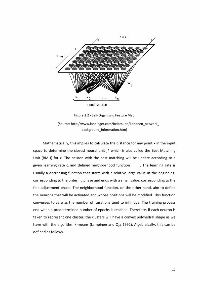
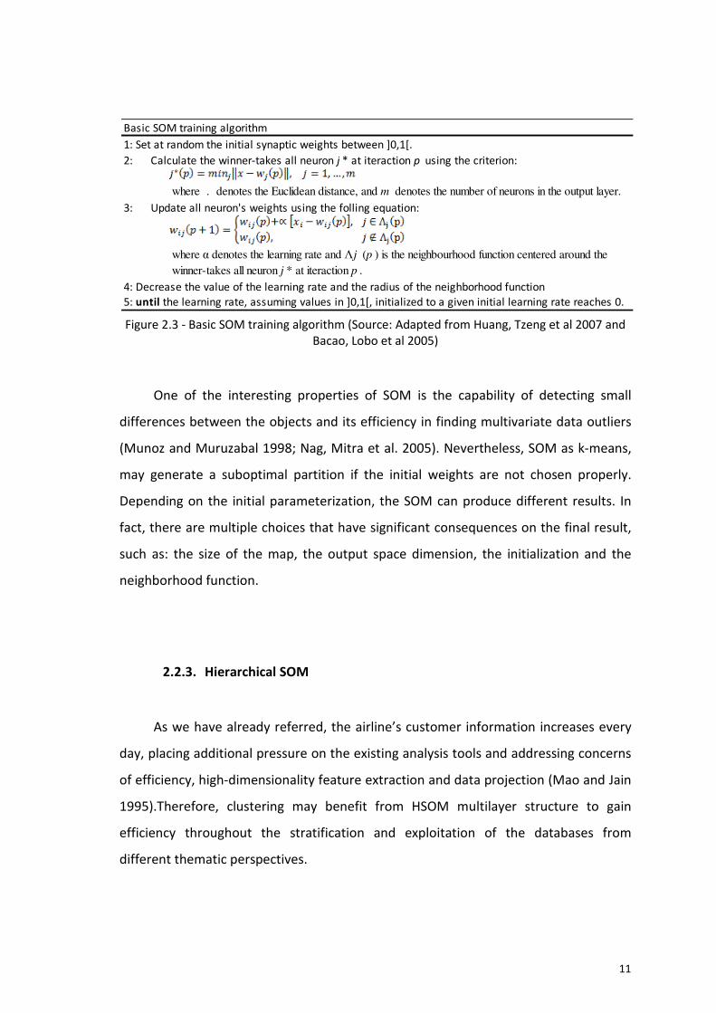
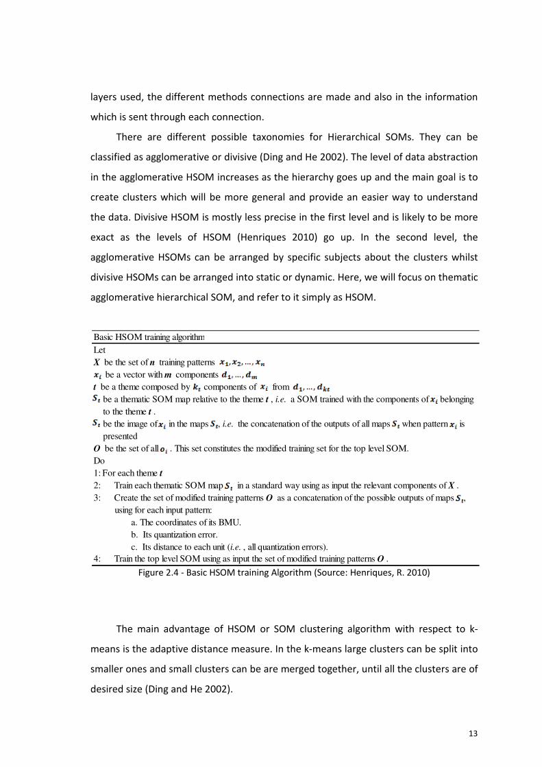

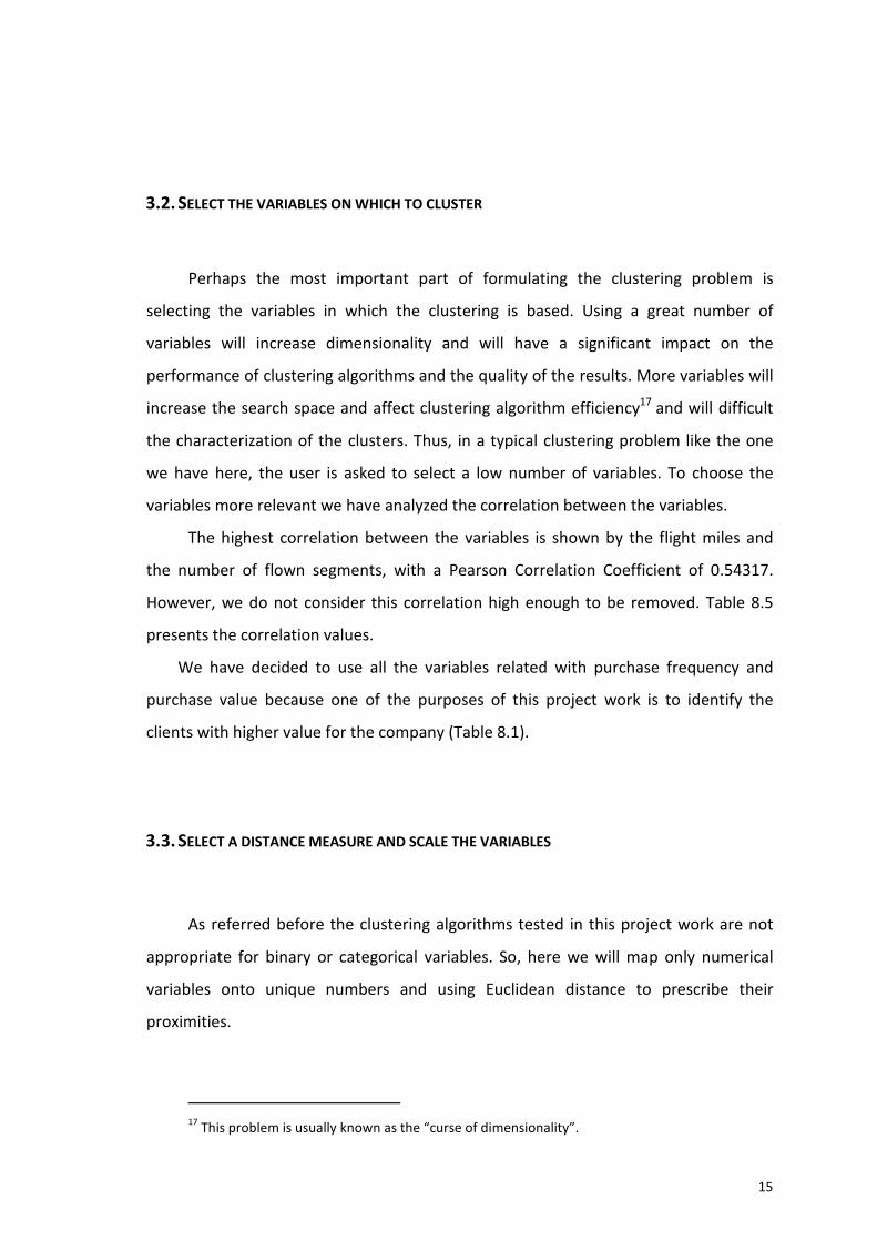
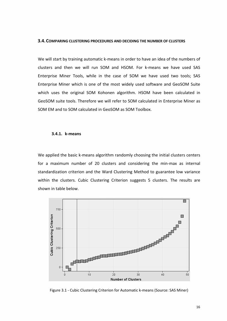

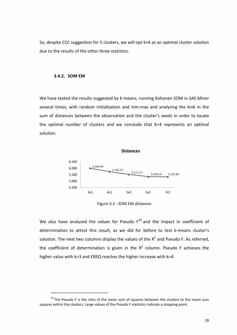


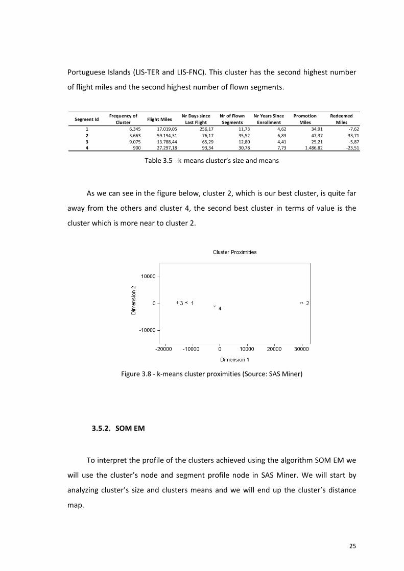


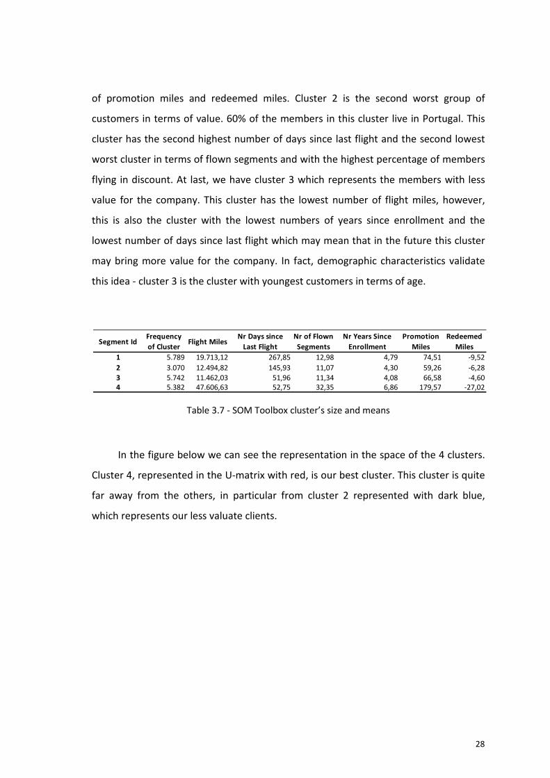
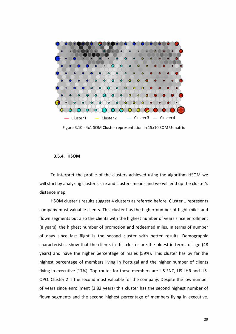


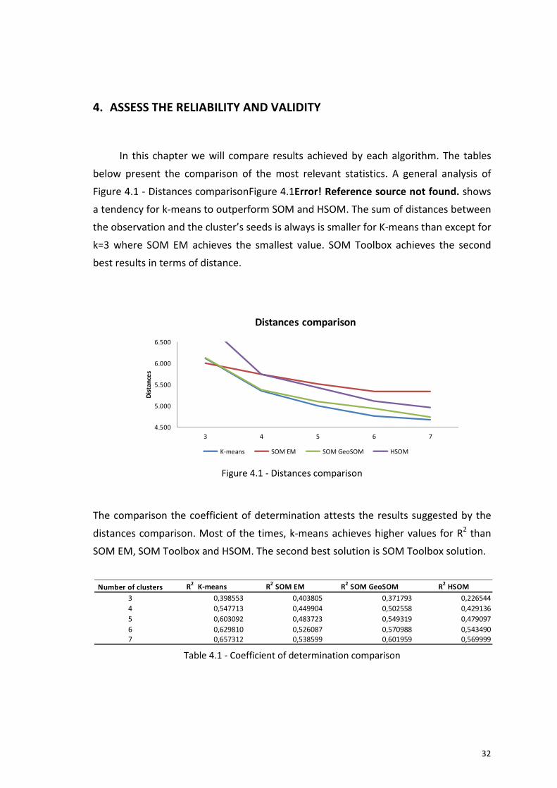


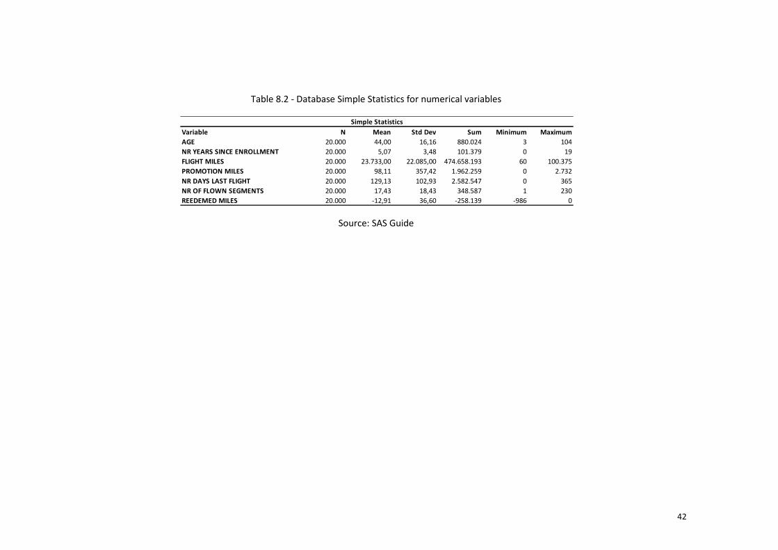


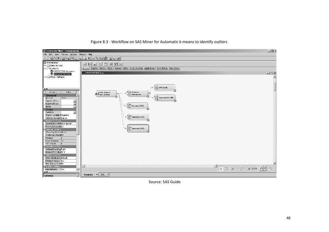


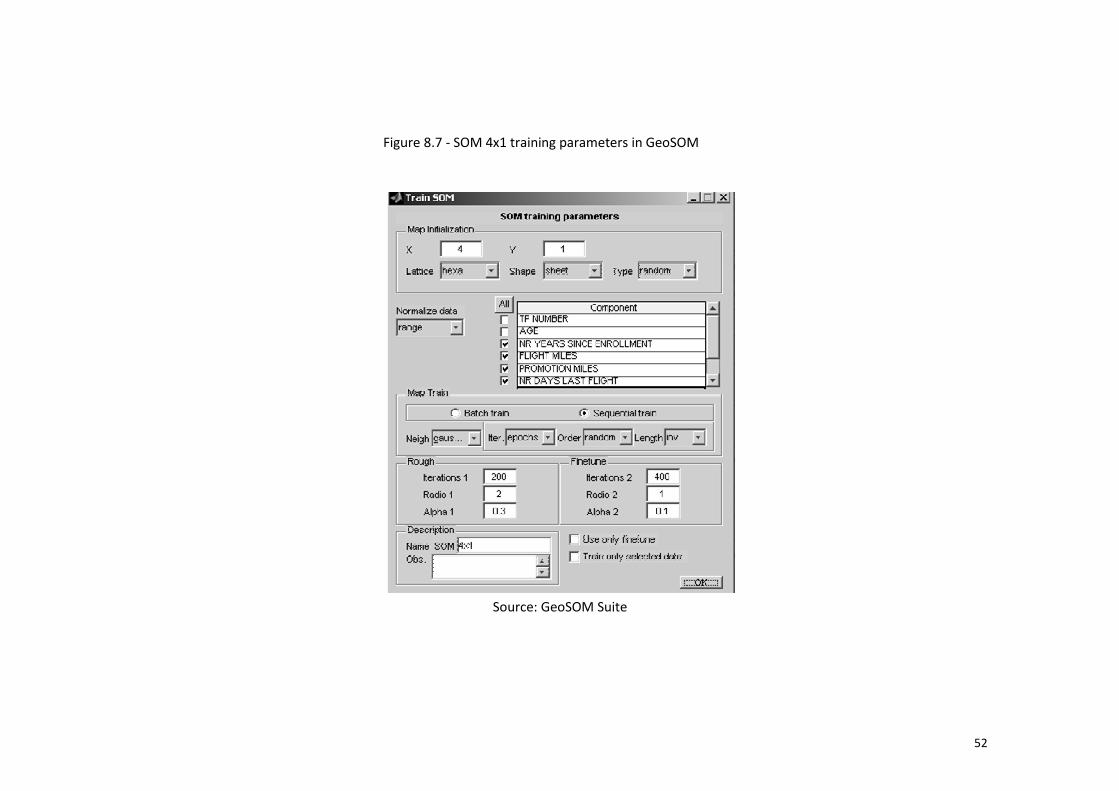
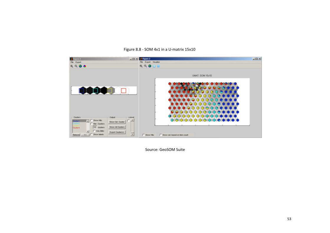
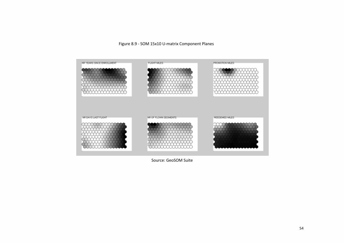
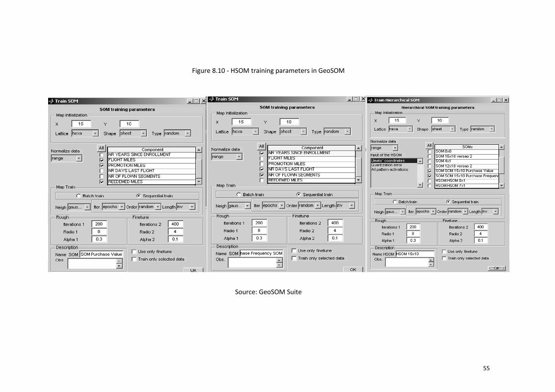


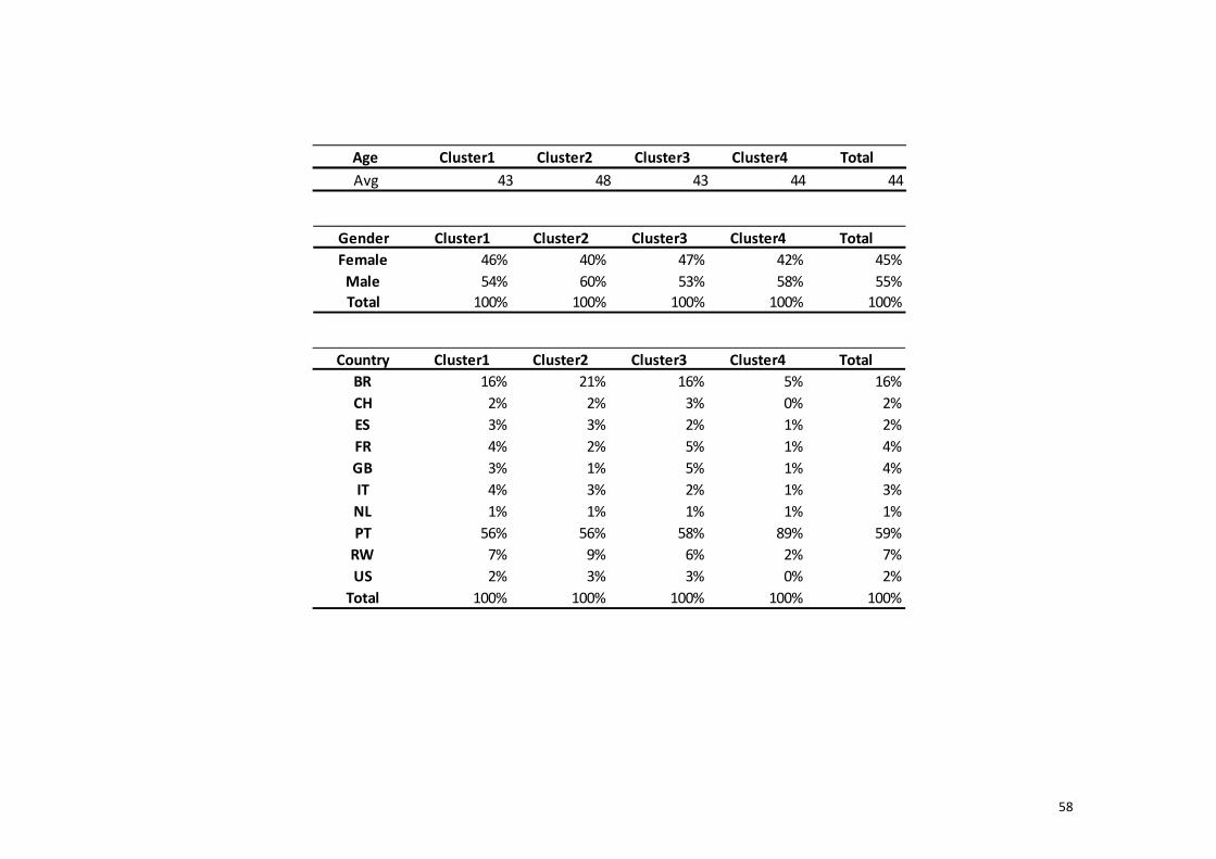

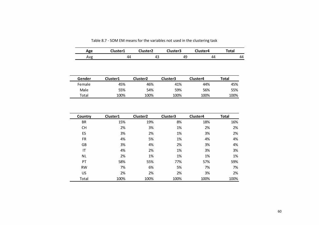


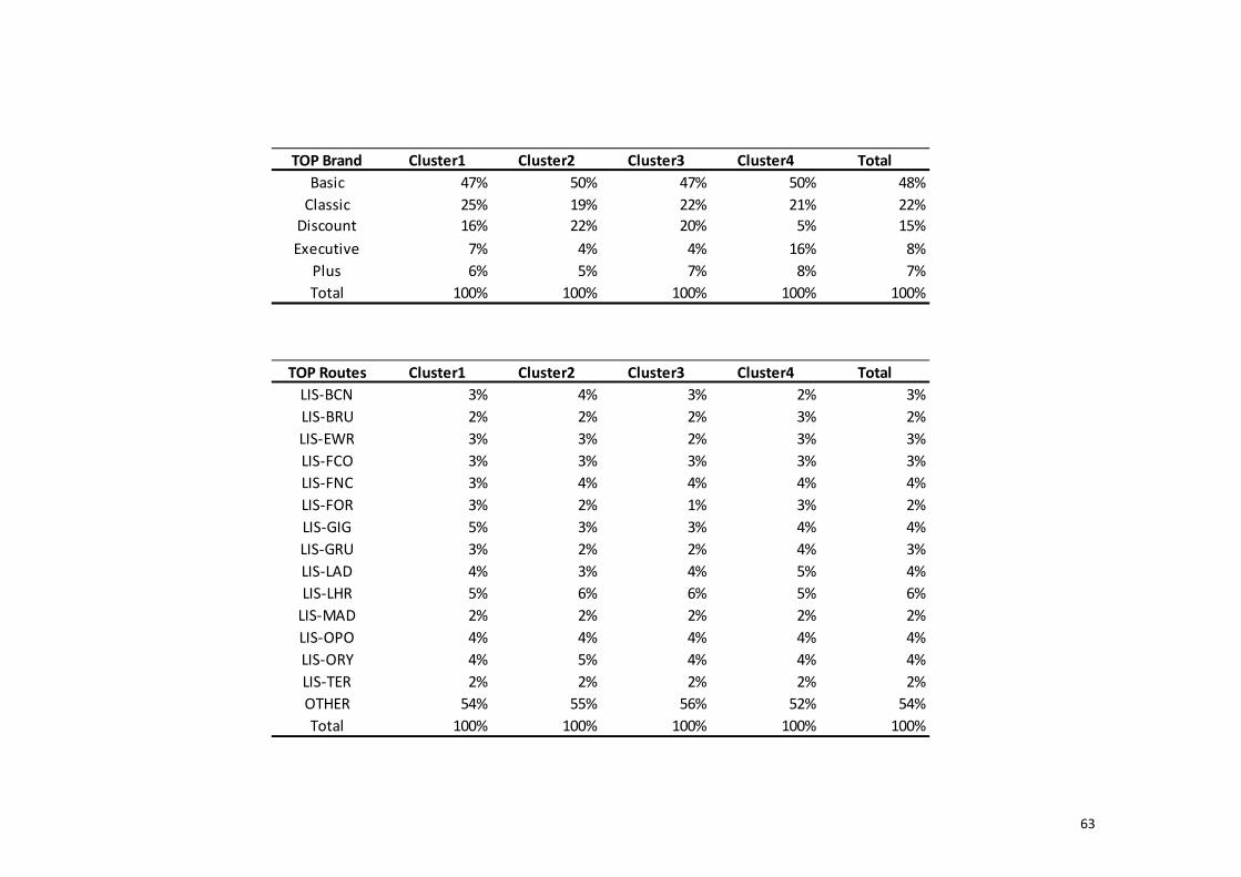


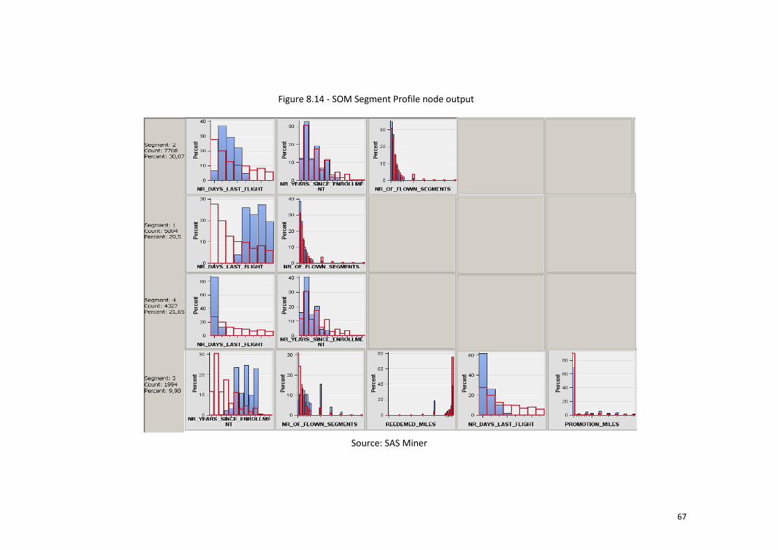


![· Web view[Título del documento] [Título del documento] [Título del documento]](https://static.documents.pub/doc/80x56/5e7e1d4ee07ed352d60dafdb/web-view-ttulo-del-documento-ttulo-del-documento-ttulo-del-documento.jpg)


