The Pennsylvania State University University of Maryland University of Virginia
Virginia Polytechnic Institute & State University West Virginia University
The Pennsylvania State University The Thomas D. Larson Pennsylvania Transportation Institute
Transportation Research Building University Park, PA 16802-4710 Phone: 814-865-1891 Fax: 814-863-3707
Tools to Support GHG Emissions Reduction: A Regional Effort
Part 1 – Carbon Footprint Estimation and Decision
Support
STATE HIGHWAY ADMINISTRATION
RESEARCH REPORT
TOOLS TO SUPPORT GHG EMISSIONS REDUCTION: A REGIONAL EFFORT
Part 1 - Carbon Footprint Estimation and Decision Support
AUTHORS
ELISE MILLER-HOOKS
SUVISH MELANTA
HAKOB AVETISYAN
UNIVERSITY OF MARYLAND
Project Number SP808B4A MAUTC-2008-01
FINAL REPORT
SEPTEMBER 2010
MD-10-SP808B4A
Martin O’Malley, Governor Anthony G. Brown, Lt. Governor
Beverly K Swaim-Staley, Secretary Neil J. Pedersen, Administrator
The contents of this report reflect the views of the authors who are responsible for the facts and the accuracy of the data presented herein. The contents do not necessarily reflect the official views or policies of the Maryland State Highway Administration, Mid-Atlantic University Transportation Center (MAUTC) or Navteq. This report does not constitute a standard, specification, or regulation.
Technical Report Documentation Page Report No. MAUTC-2008-01
2. Government Accession No. 3. Recipient's Catalog No.
4. Title and Subtitle Tools to Support GHG Emissions Reduction: A Regional Effort Part 1 - Carbon Footprint Estimation and Decision Support
5. Report Date September 26, 2010 6. Performing Organization Code
7. Author/s Elise Miller-Hooks, Suvish Melanta, Hakob Avetisyan
8. Performing Organization Report No.MD-10-SP808B4A
9. Performing Organization Name and Address University of Maryland Department of Civil and Environmental Engineering 1173 Glenn Martin Hall College Park, Maryland 20742
10. Work Unit No. (TRAIS)
11. Contract or Grant No. SP808B4A DTRT07-G-0003
12. Sponsoring Organization Name and Address Maryland State Highway Administration Office of Policy & Research 707 North Calvert Street Baltimore MD 21202 US Department of Transportation Research & Innovative Technology Admin UTC Program, RDT-30 1200 New Jersey Ave., SE Washington, DC 20590
13. Type of Report and Period Covered Final Report Draft
14. Sponsoring Agency Code (7120) STMD - MDOT/SHA
15. Supplementary Notes
16. Abstract Tools are proposed for carbon footprint estimation of transportation construction projects and decision support for construction firms that must make equipment choice and usage decisions that affect profits, project duration and greenhouse gas emissions. These tools will enable responsible agencies and construction firms to predict and affect the impact of their construction-related decisions and investments.
17. Key Words Transportation, construction, greenhouse gas, emissions, optimization
18. Distribution Statement: No restrictions This document is available from the Research Division upon request.
19. Security Classification (of this report) None
20. Security Classification (of this page) None
21. No. Of Pages 170
22. Price
Form DOT F 1700.7 (8-72) Reproduction of form and completed page is authorized.
iv
EXECUTIVE SUMMARY
The construction sector plays a significant role in worldwide greenhouse gas (GHG)
emissions. The transportation construction industry contributes to these emissions
through the burning of fossil fuels in the operation of heavy equipment, deforestation,
and release of pollutants from on-site production and use of large quantities of off-
gassing materials (e.g. asphalt and concrete). This study proposes tools for predicting or
assessing the carbon footprint of construction and maintenance projects associated with
roadways and other components of the transportation infrastructure. The developed tools
will enable responsible agencies and construction firms to predict and affect the impact of
their construction-related decisions and investments.
The first tool, the carbon footprint estimation tool (CFET), estimates the
emissions footprint of construction projects in the transportation sector. This tool
determines emissions from an inventory of equipment and construction processes, and
credits efforts to reduce emissions through reforestation and equipment retrofit, while
incorporating recent and future GHG policies on quantifying emissions. It was developed
using the state-of-the-practice methodologies available nationally and is in accordance
with global regulations under the IPCC Guidelines for National Greenhouse Gas
Inventories. The benefits of this tool lie in its wide-applicability to a variety of users, as
well as project sizes and types. Independently, this tool will enable construction
companies to identify sources and reduce emissions, while also allowing state agencies to
monitor these companies in accordance with GHG laws.
The ability to estimate emissions resulting from decisions related to equipment
usage, material choice, and site preparation produced from CFET enables the
development of an additional class of decision support tools. Specifically, an
optimization-based methodology (a decision support tool) was developed that derives
input from an emissions estimation tool to aid construction firms in making profitable
decisions in terms of equipment choice and usage while simultaneously reducing project
emissions or meeting relevant constraints imposed by recent emissions-related laws. A
myriad of programs currently exist to support efforts toward reducing emissions from
equipment use and materials production. However, it appears that no tools exist to aid
v
contractors in making optimal construction management plans with the goal of reducing
emissions while minimizing the impact on costs. This methodology helps to fill that gap.
Given the high cost of new, more efficient equipment, older, more emissive
equipment is often used on construction jobs. To encourage construction contractors to
improve their fleet mix, new jobs undertaken in the United States often require that the
equipment mix meet Environmental Protection Agency (EPA) Nonroad Diesel Tier
System guidelines. These guidelines limit the number of older, less efficient equipment
on a job site during specified periods of time. The proposed decision support tool permits
a contractor to develop an equipment-usage plan that adheres to current environmental
standards and anticipated new regulations, accounting for recent laws that might affect
construction, and possible future carbon tax or cap and trade programs. Moreover, these
tools assist contractors in trading off project cost, duration and resulting emissions in bid
development and aid contractors in making green construction decisions. They will,
likewise, allow transportation agencies to consider emissions as a factor in assessing bids.
The techniques are designed to be generic and can be applied over varying geographic
locations, site elevations, soil properties and other factors that affect equipment operation.
Collectively, the carbon footprint estimation and decision support tools were
applied to data associated with the construction of the Inter-County Connector (ICC), a
new roadway that will connect counties in Maryland. Application of the tools to this case
study showed its utility and highlighted the need for reduction strategies.
CFET used estimates made from the data provided by the ICC Contract A as
inputs and calculated the net emissions from the entire project over the duration of
Contract A (2.5 years). The tool estimated emissions from each of the processes observed
on the construction site, such as site preparation, operation of equipment and
reforestation. Additionally, the tool was able to identify sources of high and low
emissions, and quantify the sequestration capabilities attained by the ICC through
reforestation efforts. Based on the inputs, the use of equipment on site proved to be the
major GHG emitter, followed by deforestation; reforestation compensated for a small
portion of the total emissions produced on-site. The tool also calculated the offsets that
the project would require to purchase in order to achieve zero net emission status.
Analysis using the decision support tool showed that a substantial decrease in
emissions can be achieved with a relatively small increase in equipment cost. For
vi
example, in the ICC case study, it was found that a savings of 12% in emissions can be
achieved through a 0.95% increase in total cost with the use of more efficient, less
emissive equipment. The tool further aids in establishing a reasonable cap on emissions
for a given project so as to prevent excessive strain on a budget.
This work supports both local and worldwide efforts, such as those of the 193
countries that participated in the United Nations Conference on Climate Change in 2009
in Copenhagen, Denmark to reduce regional and national emissions and limit the rise of
global temperatures.
This work is part of a larger regional effort to develop tools to support GHG
emissions reduction. The regional effort is funded by the Mid-Atlantic University
Transportation Center, Maryland State Highway Administration and NAVTEQ.
vii
Table of Contents EXECUTIVE SUMMARY ............................................................................................. iv
Table of Contents ............................................................................................................ vii
List of Tables .................................................................................................................... ix
List of Figures .....................................................................................................................x
List of Appendices ............................................................................................................ xi
List of Acronyms ............................................................................................................. xii
Chapter 1. Introduction.....................................................................................................1
Chapter 2. Background .....................................................................................................3
2.1 Overview of Greenhouse Gas Emissions .................................................................. 3 2.2 Greenhouse Gas Policies and Regulations: Global and National ............................. 5 2.3 Emissions reductions: The Future ............................................................................. 6
Chapter 3. Greenhouse Gas Emissions Calculations ......................................................8
3.1 Emission Factor (EF) ................................................................................................ 8 3.2 Carbon Density (C-density) .................................................................................... 11 3.3 Measuring Greenhouse Gases: GWP and Units ..................................................... 12
3.3.1 Global Warming Potential (GWP) ................................................................... 12 3.3.2 Units of Measurement ...................................................................................... 13
3.4 Overview of Existing Estimation Models of Greenhouse Gases in the U.S. .......... 13
Chapter 4. Emissions in Construction ...........................................................................16
4.1 Emissions in the Construction Sector ..................................................................... 16 4.2 Emission Reduction Polices in Construction .......................................................... 18 4.3 Project Motivation .................................................................................................. 19
Chapter 5. Carbon Footprint Estimation Tool (CFET) for Construction Projects ..22
5.1 Description of CFET ............................................................................................... 22 5.2 Components of CFET ............................................................................................. 23 5.3. Methodology of Emissions Estimation of Components ........................................ 24
5.3.1 Site-Preparation: Deforestation & Soil Movement .......................................... 24 5.3.2 Equipment Usage ............................................................................................. 29 5.3.3 Materials Production ........................................................................................ 35
5.3.3.1 Cement and Concrete ................................................................................ 36 5.3.3.2 Asphalt ...................................................................................................... 39 5.3.3.3 Coatings & Solvents ................................................................................. 42 5.3.3.4 Fertilizers .................................................................................................. 44
viii
5.3.3.5 Steel........................................................................................................... 46 5.3.4 Environmental Impact Mitigation .................................................................... 49 5.3.5 Offsets .............................................................................................................. 53
5.4 Output ..................................................................................................................... 56
Chapter 6. A Decision Support Methodology................................................................58
6.1 Description of Decision Support Tool .................................................................... 58 6.2 Mathematical Formulation and Solution ................................................................ 59
6.2.1 Problem Formulation of OESP ........................................................................ 59 6.2.1.1 Notation Used in Problem Definition ....................................................... 60 6.2.1.2 Mathematical Definition of the OESP ...................................................... 61
6.2.2 Solving OESP .................................................................................................. 63 6.2.2.1 Weighting Method for Developing Pareto-Frontier ................................. 63 6.2.2.2 Constrained Method Given an Emissions Cap ......................................... 64
Chapter 7. ICC Case Study .............................................................................................66
7.1 Description of ICC Project...................................................................................... 66 7.2 List of Data Obtained from the ICC Project ........................................................... 67 7.3 Estimates Made from ICC Project Data for CFET ................................................. 69 7.4 Estimates Made from ICC Project Data for Decision Support Tool ...................... 71 7.5 Results & Discussion from CFET........................................................................... 75 7.6 Results & Discussion from the Application of the Decision Support Techniques . 82
7.6.1 Results .............................................................................................................. 82 7.6.2 Discussion ........................................................................................................ 89
Chapter 8. Conclusions ....................................................................................................91
APPENDIX .......................................................................................................................94
References .......................................................................................................................153
ix
List of Tables
Table 3-1. Carbon dioxide emission factors of transportation fuels. .................................. 9 Table 3-2. AP-42 ratings of emission factors established by USEPA. ............................. 10 Table 3-3. Carbon density values for various forest types in the northeast region of
the U.S............................................................................................................. 11 Table 3-4. GWP Values for some common GHGs. .......................................................... 12 Table 3-5. Common units of measurement of GHGs & their conversions. ...................... 13 Table 3-6. Summary of current models in emissions estimation & their uses. ................ 14 Table 5-1. Original data with C-density values for all carbon pools in the northeast
region. ............................................................................................................. 27 Table 5-2. Database constructed for site-preparation component of CFET from
original data with soil & non-soil carbon pools. ............................................. 27 Table 5-3. N2O emissions from forest soils. ..................................................................... 28 Table 5-4. Extrapolation trend as applied to model years 2002-2007 & rated power
based on analysis of PM standards. ................................................................ 32 Table 5-5. Fuel-based correction factors used in equipment usage emissions
calculation. ...................................................................................................... 34 Table 5-6. Calculation of emission factor for cement based on clinker type. .................. 38 Table 5-7. Percent evaporation of diluents by cutback asphalt curing type. .................... 42 Table 5-8. Density of diluents used in asphalt production emissions calculations. .......... 42 Table 5-9. Emission factors for calculation of steel production emissions. ..................... 48 Table 6-1. Maryland’s Tier System Guidelines for equipment on construction sites. ..... 60 Table 7-1. Data provided for use in case study by ICC Contract A. ................................ 68 Table 7-2. Additional input information not provided by ICC Contract A used in
decision support tool. ...................................................................................... 74 Table 7-3. Summary of results of ICC case study from CFET. ........................................ 76 Table 7-4. Contribution of equipment emissions by tier level over project period
on the ICC Contract A site. ............................................................................. 80 Table 7-5. Summary of offset determination for ICC Contract A. ................................... 81 Table 7-6. Analysis of annual sequestration rates of trees. ............................................... 82 Table 7-7. Number of equipment pieces assigned by tier for t=21. .................................. 86 Table 7-8. Number of equipment pieces assigned by equipment type and category
for t= 21 . ........................................................................................................ 86 Table 7-9. Costs comparison by Ω for a carbon price of $5/MT. ..................................... 87 Table 7-10. Equipment and total cost increases compared with cost for Ω = 1. .............. 88 Table 7-11. Emission reductions compared with cost for Ω = 1. ..................................... 88
x
List of Figures
Figure 4-1. Construction industry as the 3rd largest emitter amongst all U.S.
industries. ...................................................................................................... 17 Figure 4-3. Division of emissions from construction industry by sub-sectors. ................ 18 Figure 4-2. Construction equipment as leading emitter among non-transportation
sources. .......................................................................................................... 18 Figure 4-4. Industry survey of construction firms that use emissions reduction
strategies. ....................................................................................................... 20 Figure 5-1. Diagram illustrating the various components of CFET. ................................ 23 Figure 5-2. Screenshot of the user-interface for site-preparation component. ................. 25 Figure 5-3. Screenshot of the user-interface for equipment usage component. ................ 30 Figure 5-4. Screenshot of the user-interface for cement and asphalt in materials
production component. .................................................................................. 37 Figure 5-5. Screenshot of the user-interface for coatings and solvents in materials
production component. .................................................................................. 43 Figure 5-6. Screenshot of the user-interface for fertilizers in materials production
component. .................................................................................................... 45 Figure 5-7. Screenshot of the user-interface for steel in materials production
component. .................................................................................................... 47 Figure 5-8. Screenshot of the user-interface for environmental impact mitigation
component. .................................................................................................... 50 Figure 5-9. Screenshot of the user-interface for offsets component. ................................ 54 Figure 5-10. Screenshot of user-interface of output from model. ..................................... 57 Figure 7-1. Map featuring the various segment of the ICC roadway project. .................. 67 Figure 7-2. Chart illustrating the contribution of activities on the ICC Contract A to
emissions produced. ...................................................................................... 77 Figure 7-3. Comparison of population profile to sequestration profile of
reforestation vegetation. ................................................................................ 77 Figure 7-4. Emissions profile of the ICC Contract A equipment usage by
equipment type. ............................................................................................. 78 Figure 7-5. Total emissions produced on the ICC Contract A by equipment type. .......... 79 Figure 7-6. Number of equipment piece by type on the ICC Contract A. ........................ 79 Figure 7-7. Pareto-Frontier for CO2e at $5/MT ................................................................ 83 Figure 7-8. Pareto-Frontier for CO2e at $30/MT .............................................................. 83 Figure 7-9. Pareto-Frontier for CO2e at $50/MT .............................................................. 84 Figure 7-10. Impact of reduced emissions cap on equipment cost. .................................. 85 Figure 7-11. Costs from equipment and emissions. .......................................................... 88
xi
List of Appendices
Appendix A: GWP Values for all species of air pollutants as mandated by the IPCC. .... 95 Appendix B: Nonroad exhaust emissions standards: EPA Tier System. .......................... 96 Appendix C: Database used in site-preparation component of CFET. ............................. 98 Appendix D: Summary of extrapolation trend as applied to model year & rated
power in equipment usage emission factor database. ............................... 103 Appendix E: Analysis of EPA Tier System’s PM standards used to determine
extrapolation trend for equipment usage emission factor database. .......... 104 Appendix F: Intermediary database used to estimate median model year by tier
level based on the EPA Tier System. ......................................................... 107 Appendix G: Example of emission factor database for equipment usage component
(2006) of carbon footprint estimation model. .......................................... 109 Appendix H: Calculation of fuel-based correction factors used in equipment usage
emissions component. .............................................................................. 118 Appendix I: Typical coatings/solvents & their percent solids and density data. ............ 119 Appendix J: N-content of some common fertilizers used in materials production
component .................................................................................................. 120 Appendix K: Database used in environmental impact mitigation component of
CFET. ....................................................................................................... 121 Appendix L: Classification of tree species and database used in offset component
of CFET. .................................................................................................... 130 Table L-1. Classification of common trees used in reforestation. ........................ 130 Table L-2. Database used in the offset component. ............................................. 131
Appendix M: ICC input data & emissions calculation for equipment usage component of CFET. ................................................................................ 133
Table M-1. ICC equipment inventory as processed to fit analogous equipment categories CFET. ............................................................. 133
Table M- 2. Results from emissions calculation of the ICC equipment fleet. ..... 140 Appendix N: ICC input data & emissions calculation for site-preparation
component of CFET. ................................................................................ 148 Appendix O: ICC input data & emissions calculation for materials component
of CFET. .................................................................................................... 149 Appendix P: ICC input data & emissions calculation for environmental impact
mitigation of CFET. ................................................................................... 150 Appendix Q. List of selected equipment given by solution of OESP with the
given Ω and t=21. ...................................................................................... 152
xii
List of Acronyms Acronym ACES American Clean Energy and Security Act ARB Air and Resource Board (under U.S. state of California) ARRA American Recovery and Reinvestment Act of 2009 BOF Basic Oxygen Furnace C stock Carbon stock CDM Clean Development Mechanism CAR Climate Action Report (developed by U.S. Government) CCSP Climate Change Science Program CCTP Climate Change Technology Program CCX Chicago Climate Exchange C-density Carbon density CEMS Continuous emission monitoring system CER Certified Emissions Reduction CH4 Methane CO Carbon monoxide CO2 Carbon dioxide CO2e Carbon dioxide equivalent COP15 United Nations Conference on Climate Change CORINAIR Core Inventory of Air Emissions in Europe DOE Department of Energy (under U.S. Government) DOT Department of Transportation (under U.S. Government) EAF Electric Arc Furnace ECMT European Conference of Ministers of Transport EF Emission factor EFDB Emission factor database ( by IPCC) EIIP Emissions Inventory Improvement Program ( by EPA) EPA Environmental Protection Agency (under U.S. Government) FIADB Forest Inventory and Analysis Database (by USDA) GHG Greenhouse Gas GWP Global warming potential ha Hectare hp Horsepower ICC Inter County Connector IPCC International Panel on Climate Changes (under UNFCCC) kg Kilogram
xiii
L Liters LSD Low sulfur diesel (550 ppm) M2M Methane to Markets MC Medium cure asphalt MD State of Maryland MMT Million metric tons MT Metric tons N Nitrogen N2O Nitrous dioxide
NASA National Aeronautics and Space Administration (under the U.S. Government)
NCDC National Clean Diesel Campaign by EPA NO Nitric oxide NOx Nitrogen oxides O2 Oxygen O3 Ozone OHF Open Hearth Furnace OTAQ Office of Transportation and Air Quality (under U.S. Government) PM Particulate matter ppm Parts per million RC Rapid cure asphalt RGGI Regional Greenhouse Gas Initiative ROG Reactive organic gas SC Slow cure asphalt SHA State Highway Administration (of MD) SOC Soil organic carbon SOx Sulfur oxides U.S. United States of America ULSD Ultra low sulfur diesel (15 ppm) UNFCCC United Nations Framework Convention on Climate Change USDA Unites States Department of Agriculture VOC Volatile organic content WHO World Health Organization (under United Nations)
1
Chapter 1. Introduction
The turn of the 21st Century saw the world population rise to approximately 6.7
billion, of which the United States accounts for almost five percent [U.S Census Bureau,
2009]. This exponential growth has created an increased demand on energy and other natural
resources, resulting in wide-spread impact on the environment. Growing awareness of the
impact of greenhouse gas (GHG) emissions produced by humans on climate change has
brought critical attention towards developing strategies to identify their sources, and to
estimate and reduce their magnitude. This project aids in the estimation and reduction of
GHG emissions in construction projects associated with roadways and other components of
the transportation infrastructure. The objective was to conceptualize and build tools that will
enable responsible agencies to assess and predict the impact of their construction-related
decisions and investments. Specifically, an emissions estimation tool was developed to
quantify the carbon footprint of these construction efforts. In addition, optimization-based
techniques that derive input from this emissions assessment tool were created to aid
construction firms in making profitable decisions in terms of equipment choice and usage
while simultaneously meeting relevant constraints imposed by recent emissions-related laws.
While GHGs are vital to life on earth to help regulate surface temperatures and the
climate, constant deposition through human activities in the past decades has resulted in
excessive concentrations in the atmosphere causing global warming. Global warming is
known to have several environmental (e.g. melting of polar ice, increased frequency of
severe weather events, etc.,) and health effects. With the intention of reversing the effects of
climate change, global and national agencies have developed and continue to develop
regulatory policies, such as the Kyoto Protocol and the American Recovery and
Reinvestment Act, to reduce emissions. Chapter 2 presents an overview of GHGs, its sources
and the general effects of climate change. Current and future polices in relation to GHG
reduction are also discussed in this chapter.
The common methods of calculating GHG emissions are based on an emission factor
and conversion to carbon dioxide equivalents (CO2e). They are presented in Chapter 3.
Existing models employed in carbon emissions estimation are also reviewed.
2
Chapter 4 focuses on emissions in the construction industry in the United States
(U.S.) and the impact of specific governmental emissions reduction strategies on the
industry. Many of these strategies, like the U.S. Environmental Protection Agency’s (EPA)
Clean Air Nonroad Diesel Rule, have already been implemented and are establishing
standards for the management of construction projects. This chapter introduces the
motivation behind this research and project, since construction agencies will be required to
evolve in their methods to meet these strict standards.
Chapter 5 describes in detail the methodologies and assumptions used to develop the
carbon footprint estimation tool proposed herein. The carbon estimation tool will determine
emissions from operation of an inventory of applicable equipment (type, brand and age), and
construction processes (site preparation, materials productions, etc.), while crediting any
efforts to reduce GHG emissions through reforestation or equipment retrofit. The tool also
incorporates recent and future GHG policies on quantifying emissions.
In Chapter 6, optimization-based techniques are proposed that derive input from the
emissions estimation model presented in Chapter 5. Mathematical models were formulated to
generate optimal or Pareto-optimal decisions in terms of equipment choice and usage
simultaneous with reducing project emissions or meeting relevant constraints imposed by
recent emissions-related laws. These models are intended for use by construction firms in
making profitable, but green decisions.
The tools were applied to data obtained from the Intercounty Connector (ICC) project
as a case study to evaluate their utility and efficiency in Chapter 7.
The developed tools enable construction companies to actively reduce emissions and
optimize the construction process and costs. Simultaneously, these tools will allow state
agencies to monitor these companies in accordance with recent GHG reduction laws at both
state and federal levels. These and other benefits are described in Chapter 8. A discussion of
potential uses of the developed tools beyond transportation infrastructure construction is also
provided.
3
Chapter 2. Background
2.1 Overview of Greenhouse Gas Emissions
Greenhouse effect is a natural phenomenon that is induced when atmospheric gases
trap the ultraviolet rays from the sun within the earth’s atmosphere. It is therefore essential in
maintaining the earth’s temperature and climatic conditions. Naturally occurring
atmospheric gases such as water vapor, carbon-dioxide (CO2), nitrous oxide (N2O), methane
(CH4), ozone (O3) and, anthropogenic-produced gases such as halocarbons, nitric oxide
(NO), carbon-monoxide (CO), aerosols, and fluorinated gases are collectively classified as
greenhouse gases (GHGs). Additionally, other air pollutants such as sulfur oxides (SOx),
reactive organic gases (ROG) and particulate matter (PM) also indirectly affect greenhouse
gas effect [USEPA, 2010c].
CO2 is produced primarily from the combustion of fossil fuels, like petroleum, diesel
and biofuels, and biomass, such as trees and solid wastes as a result of their high carbon
content. It is also formed naturally during biological respiration and artificially during the
production of materials, like cement, steel, asphalt and chemicals. CO2 is sequestered through
the natural carbon cycle by forests and oceans. CH4 is emitted from the burning of fuels as
well, in addition to being produced from livestock, agricultural practices and decay of
organic material [USEPA, 2010c]. NO and NO2, the primary constituents of NOx emissions,
are formed when nitrogen (N), either in the air or in fuel, combines with oxygen (O2) at high
temperatures. Other pollutants, such as PM and CO, are formed as a result of incomplete
combustion of fuel; whereas, SOx are formed from the sulfur content in the fuel [USEPA,
2009b].
Although the earth produces GHGs through natural processes, such as respiration of
plants and animals, volcanic eruptions and regular changes in temperatures, the concentration
of these gases in the atmosphere is maintained through natural absorption by forests and
oceans. However, since the industrial revolution, anthropogenic activities, such as use of
fossil fuels, and deforestation for urbanization and agriculture, have resulted in an increased
deposition of these gases into the atmosphere [IPCC, 2007]. The International Panel on
Climate Change (IPCC) has established a strong correlation between the anthropogenic
4
deposition of GHGs and global warming resulting in climate change. Due to its large
volumetric prevalence, CO2 is considered a major player in elevating greenhouse effect, and
accounts for approximately 86% of all U.S. emissions. CO2 emissions are increasing at a rate
of about 0.3% per year, resulting in almost a 36% total increase since the Industrial
Revolution [USEPA, 2009a]. The excessive presence of GHGs, further worsened by the
constant growth in population, magnifies the greenhouse effect, thereby raising the earth’s
temperature and bringing about ‘global warming’. Global warming is a result of the
exacerbation of the earth’s greenhouse effect.
Some of the observed effects of climate change include increase in the earth’s
temperatures, melting of the glacial ice-caps, rise in sea level, and variations in the length of
seasons. Recent years (1995 to 2006) have been recorded to be the warmest years since 1850.
The warmer temperatures are known to cause changes in regional precipitation, later freezing
and earlier break-up of ice on rivers and lakes, lengthening of growing seasons, shifts in plant
and animal ranges, and earlier flowering of trees. The sea level has been predicted to rise
between seven and twenty-three inches by 2080, posing increased risk of loss of land and
habitats, and danger to human population in coastal areas. Moreover, the changes in climatic
conditions have increased the probability and intensity of extreme climatic events, such as
hurricanes, droughts, wildfires and other natural disasters, resulting in damage to human
lives, property and the nation’s economy [IPCC, 2007].
Beside the environmental effects, climate change is also known to affect human
health directly from exposure to heat-waves or cold fronts, and the lengthening of
transmission seasons of vector borne diseases that thrive in warm temperatures. Decreased
air quality has contributed to increased incidence of respiratory diseases and damage to lung
tissue [WHO, 2003].
Although each of the GHGs have varying effects on the environment and human
health, it is critical that their concentrations in the atmosphere be reduced to curb climate
change and, therefore, preserve the earth for future generations.
5
2.2 Greenhouse Gas Policies and Regulations: Global and National
The United Nations Framework Convention on Climate Change (UNFCCC) was
developed in 1994 to address the urgent need to reduce GHG emissions and, thus, curb
climate change. 193 nations collectively established the Framework’s objective of
“…stabilization of greenhouse gas concentrations in the atmosphere at a level that would
prevent dangerous anthropogenic interference with the climate system” [ECMT, 2007]. In
1997, the UNFCCC members drew up the Kyoto Protocol, an international binding
agreement signed by 37 industrialized countries and ratified by 55 nations (not including the
U.S.), all committing to reduce GHG emissions to 5% below their 1990 levels by 2012. The
Framework presents market-based strategies, such as emission trading, clean development
mechanisms and joint implementation to help participants implement the Protocol. Although
the Framework provides these global options, it strongly encourages that national measures
be taken [UNFCCC, 2010].
Under its commitment to the UNFCCC, the U.S. government develops a national
emissions inventory annually, recording sources and sinks of emissions from various sectors
of the economy. These inventories are developed in accordance with the guidelines
established by the IPCC. Additionally, the State Department authors the annual Climate
Action Report documenting current climatic conditions, GHG emissions, policies and
regulations [U.S. Department of State, 2006].
Within the U.S., the government collaborates with several federal agencies, such as
the Environmental Protection Agency (EPA), Department of Energy (DOE), Department of
Transportation (DOT), Department of Agriculture (USDA) and National Aeronautics and
Space Administration (NASA), in efforts to monitor and reduce emissions. However, most of
these efforts are executed under the close guidance of the USEPA.
In its efforts to abate emissions, the government has developed initiatives/programs,
some of which facilitate technological and informational exchange, while others provide
financial incentives. One of the notable informational exchange initiatives is the Climate
VISION Partnership established between major industrial sectors (e.g. oil and gas,
transportation, electricity generation, mining, manufacturing and forestry products) and four
U.S agencies (DOE, EPA, USDA, and DOT) to reduce GHG emissions in the next decade.
6
Similarly, the Clean Energy-Environment State Partnership Program and the Climate Leaders
program are collaborations between EPA and states, and private companies, respectively, to
encourage goals and establish concrete strategies towards emissions reduction. Other
initiatives, like ENERGYSTAR buildings and Green Power Partnerships, deal with reduction
of emissions through improving energy efficiency. The Climate Change Technology
Program (CCTP) and the Climate Change Science Program (CCSP) are initiatives that
revolve around the development of clean technology and the improvement in the
understanding of the science behind climate change [USEPA, 2010c].
2.3 Emissions reductions: The Future
As the awareness of global warming continues to grow, political and public
sentiments have been increasing towards employing strategies that promote clean
development and, thereby, reduce national emissions. Being the North American country that
ranks as the top emitter per capita worldwide, the U.S. contributes almost 19.4% of global
emissions but only accounts for 5% of global population [IPCC, 2007]. This has resulted in a
watchful eye towards U.S. efforts in reducing its emissions. Moreover, in the recent 2009
United Nations Conference on Climate Change (COP15), the U.S. developed the
Copenhagen Change Accord in collaboration with other top emitters in the world (China,
Brazil, India and South Africa) to set forth the groundwork for global action against climate
change. According to the Accord, the U.S. pledged a 17% decrease of its 2005 levels by
2020.
Already under the Obama Administration, the energy provisions of the American
Recovery and Reinvestment Act of 2009 (ARRA) promotes emissions reduction through
energy efficiency. The $787 billion Act not only provides tax incentives for use of renewable
energy and energy-efficient technologies, but also grants, contracts and loans for programs in
energy-efficiency. Under this act, with approximately $300 million in financial assistance,
the EPA strengthened the National Clean Diesel Campaign (NCDC) [ARRA, 2009].
Therefore, the U.S. government is exploring various federal and state legislative options
towards wide-spread emissions reduction. These include, but are not restricted to, enforcing a
carbon tax and/ or carbon trading system, and carbon allowances [UNFCC COP15, 2009].
7
Besides technological advancement in carbon reduction, governments are considering
instituting limitations, in the form of caps, on carbon emissions. Such caps, once enforced,
will require companies to either comply with national or regional regulations, and/or pay a
penalty for noncompliance or excessive GHG emissions production. National efforts to
reduce emissions include the set-up of partnerships to implement cap-and-trade programs.
Seven U.S. states in the Northeast and Mid-Atlantic regions have set up a regional mandatory
cap-and-trade market system called Regional Greenhouse Gas Initiative (RGGI) that aims to
reduce emissions from the power sector by 10% by 2018 and sell carbon offsets. Proceeds
from this effort are channeled to various clean energy projects [RGGI, 2009]. Several U.S.
states have since established local carbon markets that allow individuals and businesses to
purchase and sell carbon offsets. The Maryland Terrapass and Chicago Climate Exchange
(CCX) are two examples of state based carbon trading programs [MD Terrapass, 2010 &
CCX, 2010]. Other market-based emissions reductions programs include the Methane to
Markets (M2M) initiative chaired by the EPA. This global program focuses on the recovery
and sale of CH4 as clean energy [USEPA, 2010b]. While carbon markets that permit the
buying and selling of carbon allowances between companies, industries and countries
successfully exist internationally, the wide-spread establishment of such markets in the U.S.
is likely to have a significant effect on all sectors of the economy.
With several of these global and national policies as a foundation, the world has
begun to set the stage to develop stringent programs to combat climate change. This in turn
will have an effect on the future functioning of business across the world.
8
Chapter 3. Greenhouse Gas Emissions Calculations
3.1 Emission Factor (EF) The quantification of emissions is vital in the management of air quality. Emissions
estimates help identify key sources and enable the development of strategic tools to combat
poor air quality. Emissions are determined via the use of an appropriate emission factor (EF).
An EF is “a representative value that relates the quantity of pollutant released to the
atmosphere with an activity associated with the release of that pollutant” [USEPA, 2010c].
EFs are typically long-term averages developed from published technical data,
documentation from emission tests or continuous emission monitoring systems (CEMS) and
personal communication. Since the development of EFs is dependent on the data available,
their accuracy is sometimes imperfect. Hence, the use of an EF in quantifying emissions is at
best an approximation unless based on long-term empirical data [USEPA, 1997]. Table 3-1
lists well known EFs for a variety of fuels used in transportation.
Several EF databases are maintained globally and nationally to facilitate agencies,
industries, consultants, and other users in estimating emissions. The IPCC manages an EF
database (EFDB) library based on The Core Inventory of Air Emissions in Europe
(CORINAIR). The EFDB allows the user to obtain EFs based on IPCC source/sink
categories, which include energy, land use change, solvents, industries, etc. [IPCC-NGGIP,
2009].
EPA’s AP-42 document is a compilation of EFs for air pollutants used within the U.S.
Several website databases, such as CHIEF and FIRE, access EFs from the AP-42 and related
documents. Many U.S. states have also developed similar software models and documents
for the purpose of producing state emissions inventories [USEPA, 2010c].
EFs are ranked based on their methods and the expanse of the data used in their
development. The EPA AP-42 EF ratings are assigned as in Table 3-2.
9
Table 3-1. Carbon dioxide emission factors of transportation fuels. Source: EIA, 2010
Transportation Fuel
Emission Factors Pounds CO2 per Unit of
Volume Kilograms CO2 Per
Million BTU Aviation Gasoline 18.33 per gallon 69.16 Biodiesel
B100 0 per gallon 0.00 B20 17.89 per gallon 59.44 B10 20.13 per gallon 66.35 B5 21.25 per gallon 69.76 B2 21.92 per gallon 71.8
Diesel Fuel (No.1 and No.2) 22.37 per gallon 73.15 Ethanol/Ethanol Blends
E100 0 per gallon 0.00 E85 2.93 per gallon 14.71 E10 (Gasohol) 17.59 per gallon 65.94
Methanol/Methanol Fuels M85 10.68 per gallon 64.01
Motor Gasoline 19.54 per gallon 70.88 Jet Fuel, Kerosene 21.09 per gallon 70.88 Natural Gas 120.36 per 1000 cubic feet 53.06 Propane 12.67 per gallon 63.07 Residual Fuel (No.5 and No.6 Fuel Oil) 26.00 per gallon 78.8
10
Table 3-2. AP-42 ratings of emission factors established by USEPA. Source: USEPA, 2009b Rating Quality Assignment Analysis
A Excellent
Excellent. Emission factor is developed primarily from A and B rated source test data taken from many randomly chosen facilities in the industry population. The source category population is sufficiently specific to minimize variability.
B Above Average
Emission factor is developed primarily from A or B rated test data from a moderate number of facilities. Although no specific bias is evident, is not clear if the facilities tested represent a random sample of the industry. As with the A rating, the source category population is sufficiently specific to minimize variability.
C Average
Emission factor is developed primarily from A, B, and C rated test data from a reasonable number of facilities. Although no specific bias is evident, it is not clear if the facilities tested represent a random sample of the industry. As with the A rating, the source category population is sufficiently specific to minimize variability.
D Below Average
Emission factor is developed primarily from A, B and C rated test data from a small number of facilities, and there may be reason to suspect that these facilities do not represent a random sample of the industry. There also may be evidence of variability within the source population.
E Poor
Factor is developed from C and D rated test data from a very few number of facilities, and there may be reason to suspect that the facilities tested do not represent a random sample of the industry. There also may be evidence of variability within the source category population.
U Unrated
Unrated (only used in the L&E documents). Emission factor is developed from source tests which have not been thoroughly evaluated, research papers, modeling data, or other sources that may lack supporting documentation. The data are not necessarily "poor," but there is not enough information to rate the factors according to the rating protocol. "U" ratings are commonly found in L&E documents and FIRE rather than in AP 42.
11
3.2 Carbon Density (C-density)
CO2 is constantly cycled between the atmosphere and forest systems. Trees
continually absorb CO2 from the atmosphere via photosynthesis to grow and store it in the
form of carbon in the biomass of the tree (leaves, trunk, roots, etc.). CO2 is also stored as
carbon in soil, which accumulates when organic matter decomposes. Most soil organic
carbon (SOC) is stored within the first meter depth from the soil surface. The amount of CO2
absorbed and therefore the carbon stored, depends on the tree type, age, and size, as well as
climatic conditions of the region. Together, the amount of carbon stored in the biomass and
the soil is termed the carbon stock (C-stock) of that ecosystem and is quantified by the
carbon density (C-density) of that system. C-density is, therefore, defined as the average
mass of carbon stored in the biomass of a living system per area of that system. Table 3-3
lists the C-density of the various forests types (where non-soil refers to the carbon stored in
tree parts, and soil refers to that stored in the soil) in the northeast region of the U.S.
[USEPA, 2009a].
Table 3-3. Carbon density values for various forest types in the northeast region of the U.S. Source: USEPA, 2009a
Region Forest Type Carbon Density (MT/ha)Non-Soil Soil
Northeast (CT,DE,MA,MD,ME,NH,NJ,NY,OH,PA,RI,VT,WV)
White/Red/Jack Pine 135.8 78.1 Spruce/Fir 104.2 98 Oak/Pine 127.1 66.9 Oak/Hickory 115 53.1 Elm/Ash/Cottonwood 96.2 111.7 Maple/Beech/Birch 129.4 69.6 Aspen/Birch 72.6 87.4 Minor Types & Nonstocked 80.1 82.7 All 118.2 69.7
12
3.3 Measuring Greenhouse Gases: GWP and Units
3.3.1 Global Warming Potential (GWP)
GHGs are measured qualitatively through the intensity of their effect on the earth’s
atmosphere. This intensity is determined by the GHG’s global warming potential (GWP).
GWP is defined as “the ratio of radioactive force absorbed by one unit mass of the
greenhouse gas to that of one unit mass of reference gas over a specified time period”. CO2 is
the globally accepted reference gas with a GWP of one, and GWP is typically measured for
1-, 20-, 50-, and 100-year time periods [USEPA, 2006 & IPCC, 2007]. For example, the
GHG CH4 with a 100-year GWP of 21 has 21 times the effect on the atmosphere as
compared to CO2. Table 3-4 lists the GWP values of some common GHGs. The GWPs for all
species of air pollutants as mandated by the IPCC can be found in Appendix A.
Table 3-4. GWP Values for some common GHGs. Source: IPCC, 2007
Species Chemical Formula
Lifetime (Years)
Global Warming Potential (Time Horizon)
20 years 100 years 500 yearsCarbon Dioxide CO2 Variable 1 1 1 Methane CH4 12±3 56 21 6.5 Nitrous Oxide N2O 120 280 310 170 HFC-23 CHF3 264 9100 11700 9800 Perfluoromethane CF4 50,000 4400 6500 10,000 Sulphur hexafluoride SF6 3200 16,300 23,900 34,900
In addition to being a measure of a GHG’s effect on the atmosphere, GWPs are used
to convert GHGs into carbon-dioxide equivalents (CO2e). This allows for the use of an easy
and standard unit for reporting quantities of GHGs being measured. Mass units of GHG are
converted to CO2e by multiplying the amount by its GWP. For example, 50 pounds of CH4 =
50 pounds x 21= 1,050 pounds CO2e [IPCC, 2007].
13
3.3.2 Units of Measurement The units of measurement are typically recorded in teragrams (Tg) or million metric
tons (MT). Common units of measurement and their conversions are listed in Table 3-5.
Table 3-5. Common units of measurement of GHGs & their conversions. Source: USEPA, 2005a
From To 1 metric ton of carbon equivalent = 3.667 metric tons CO2e
1 metric ton of CO2e = 0.2727 metric tons of carbon equivalent 1 teragram = 1 million metric tons 1 kilogram = 2.205 pounds
1 pound = 0.000454 metric ton 1 metric ton = 1.102 tons
The U.S. Inventory of GHGs typically accounts for CO2, CH4, CO, NO2 and
fluorinated gases emitted from various sources, while estimating GHGs in Tg CO2e.
However, since these GHGs contribute towards air pollution, several inventories of emission
estimates, especially those from vehicles, also include other pollutants, such as SOx and PM.
3.4 Overview of Existing Estimation Models of Greenhouse Gases in the U.S.
Several models currently exist that enable the quantification of GHGs and the
subsequent development of emissions inventories. Under the Clean Air Act, the EPA creates
models that estimate emissions from various sources. The NONROAD2008 model helps in
the inventory of emissions from non-road vehicles and diesel equipment whereas the recent
MOVES2010 model estimates on-road and highway vehicle emissions. On the other hand,
GLOBEIS estimates the volatile organic content (VOC), CO and soil NOx emissions from
biogenic sources [USEPA, 2010c]. The USDA developed two models, the Carbon Online
Estimator (COLE) and Carbon Calculation Tool (CCT), which estimate C-stocks and
measure carbon flux for regions in the U.S. based on forest inventory data, respectively
[USDA NRS, 2010].
Additionally, many states and private agencies develop models to estimate emissions.
14
The state of California’s Air and Resource Board (ARB) is a pioneer in developing specific
strategies and regulations towards emissions reduction. The EMFAC2007 model is one such
model that calculates emission rates from all on-road vehicles operating on the state’s roads
[ARB, 2007]. The OFFROAD2007 model, on the other hand, estimates the contribution of
emissions due to agricultural, construction, lawn and garden equipment, as well as recreation
vehicles [ARB, 2009]. California’s URBEMIS2007 model calculates project-specific air
pollution emissions for a variety of urban land-use projects. Specifically, the model estimates
NOx, ROG, CO, CO2 and PM emissions from the operation of equipment for the
construction of an urban area (e.g. residential or educational areas) and use of associated
materials (i.e. asphalt and natural gas) [Rimpo, 2007]. Table 3-6 provides a summary of the
existing GHG estimation models.
Table 3-6. Summary of current models in emissions estimation & their uses.
Emissions Type Model Name Source
Air Pollutant/
GHGs Estimated
Utility
NONROAD2008 EPA
CO, CO2, NOx, SOx, HC, PM
Non-road vehicles and diesel equipment.
URBEMIS AQMD CO, CO2 , NOx, PM, ROG
Air pollutants from construction of urban projects.
EMFAC2007 CaliforniaARB
CO, CO2, NOx, SOx, HC, PM, Lead
On-road vehicles in California.
OFFROAD2007 CaliforniaARB
CO, CO2, NOx, SOx, HC, PM
Agricultural, construction, lawn and garden equipment, and recreation vehicles.
Biogenic GLOBEIS EPA
VOC, CO and soil NOx
Emissions from biogenic sources.
COLE USDA Carbon Tool for forest carbon analysis.
CCT USDA Carbon Stock
State-level annualized estimates of carbon stocks on forestland.
15
The majority of these models determine individual source emissions (e.g. passenger
cars) and rarely determine comprehensive emissions for a source category (e.g.
transportation). Therefore, there exists a need for an all-encompassing emissions estimation
model that will enable users to quantify emissions from various sources simultaneously. This,
in turn, will encourage and support proactive efforts in GHG emission reduction.
16
Chapter 4. Emissions in Construction
4.1 Emissions in the Construction Sector
The 873.1 billion U.S. dollar construction industry (2003) in the U.S. ranks first
among 55 nations globally [USEPA, 2008]. The industry is vital in the development of the
nation’s infrastructure, which includes construction of residential and industrial buildings,
roads, bridges and other long-standing structures. Within the U.S., this industry permeates
both the transportation and industrial sectors as it involves the use of non-road vehicles and
equipment, like excavators and cranes, and supports large construction-based industries, like
cement and chemicals. The transportation and industry sectors contribute almost 28% and
33% to U.S. national emissions, respectively. Collectively, emissions from the construction
industry amount to nearly 2% (~131 MMT CO2e) of the total U.S. emissions (Figure 4-1)
[USEPA, 2008]. Despite the economic recession, it has been estimated that by 2030, about
half of the buildings in America will have been built after 2000, implying that half the
volume of urban structures will be constructed within 25 years just to support population
growth [Nelson, 2004]. While each individual construction project may not produce large
quantities of GHGs compared with operations in other sectors, because there are consistently
a large number of on-going construction projects, the aggregate product of these projects is
large [Truitt, 2009]. The construction industry is the third largest industrial emitter of CO2
(Figure 4-1) [USEPA, 2008].
A majority of construction emissions result from either the use of fuel for operating
equipment and vehicles, or production of electricity in the transportation segment of the
construction sector [USEPA, 2009d].
17
Figure 4-1. Construction industry as the 3rd largest emitter amongst all U.S. industries. Source: USEPA, 2009d
The transportation sector in the U.S. is divided into transportation vehicles (on– and
non-road) and non-transportation vehicles. Transportation vehicles include cars, motorcycles,
light and heavy trucks, buses, ships and aircraft, among others; non-transportation vehicles
include construction, agricultural and commercial equipment, generators and recreational
vehicles [USEPA, 2009e]. The construction industry’s contribution to GHG emissions within
this sector is, in large part, like on-road traffic, due to its dependence on fossil fuel for energy
required to operate heavy equipment. However, the average rate of production of emissions
is much greater for construction equipment (i.e. non-road vehicles) as compared to passenger
vehicles (see Report MS-12 1997 for more detail) due to differences in fuel type (i.e. diesel
versus gasoline), engine technology, and horse power. For example, one can estimate that a
typical excavator produces 454 pounds of CO2e per hour of operation, while a typical
medium-size passenger vehicle (or sports utility vehicle) produces 55 (or 78.5) pounds of
CO2e per hour of operation. With continuing demand for fossil fuel, sustained increase in
GHG emissions is predicted [USEPA, 2010c]. As seen in Figure 4-2, construction equipment
contributes significantly towards the emissions from non-transportation vehicles, resulting in
2% or approximately 59.7 MMT CO2e of the transportation emissions [OTAQ, 2006].
18
The remainder of the 131 MMT CO2e of the total construction emissions stems from
the use of electricity and off-gassing from industrial processes in the construction industry,
including cement and materials production, and use of chemicals and steel. These processes
are particularly important while considering emissions due to the construction of buildings,
and heavy and civil engineering subsectors of the industry (Figure 4-3) [USEPA, 2009d].
In addition, the construction industry reduces emission sinks as building of structures
often call for deforestation of standing forests, which are important sources of atmospheric
carbon sequestration.
4.2 Emission Reduction Polices in Construction
To foster mitigation efforts to reduce industrial and construction-related
environmental impact associated with GHG emissions, improvements in technologies to aid
in monitoring, and methods to encourage individual and institutional accountability towards
emissions reductions, are being developed. The Office of Transportation and Air Quality
(OTAQ) has established programs that have already produced wide-scale reductions. Some
of these programs directly impact or regulate the construction industry. The most evident of
these is the National Clean Diesel Campaign (NCDC) that promotes immediate improvement
Figure 4‐3. Division of emissions from construction industry by sub‐sectors. Source: USEPA, 2009d
Figure 4‐2. Construction equipment as leading emitter among non‐transportation sources. Source: OTAQ 2006
19
in air quality from diesel engines through various regulatory and voluntary strategies. The
voluntary Diesel Retrofit Technology Verification Program provides agencies a list of retrofit
technologies approved by the EPA. The technologies typically enable reductions of
emissions between 20 and 90%. However, it is the NCDC regulatory programs that have had
the most impact. The Clean Air Nonroad Diesel Rule establishes a set of standards mandated
by the EPA towards reductions of emissions from diesel engines by almost 90%. The EPA
has also established a tier system, and enforces the use of low sulfur diesel in heavy-duty
engines.
The EPA’s tier system regulates emissions from diesel engines based on the
equipment age and horsepower (Appendix B). The system has four levels: tier 1, 2, 3 and 4.
Conceptually, a tier 1 level vehicle would be older and produce greater emissions as
compared to a tier 4 level vehicle. Although not strictly mandated, EPA strongly encourages
construction projects to utilize higher tiered equipment so as to reduce construction
emissions. This would imply that either the construction equipment fleet should be relatively
new or the older equipment must be retrofit with reduction technologies. Also, according to
these standards, manufacturers would be required to meet the most recent set of emissions
standards put forth by the EPA. The ultra-low sulfur diesel (ULSD) produces a 99%
reduction of the sulfur content in the fuel, reducing from current levels of 3300 parts per
million (ppm) to 15 ppm. The most updated tier system took effect in 2008; the diesel fuel
rule will be executed starting in 2010 [USEPA, 2009c].
4.3 Project Motivation
Currently, construction emissions are only calculated to develop state and national
inventories. Also, traditional approaches for construction planning do not consider emissions
as a decision factor. Studies have shown that almost 53% of survey respondents do not
employ any form of emissions reduction strategies (Figure 4-4) [USEPA, 2008]. This is
mainly because the development and installation of lower emitting vehicle technology is
time-consuming, expensive, and sometimes creates unfavorable trade-offs between cost,
productivity and emissions. Similarly, green efforts or environmental restoration involves
permitting processes that are tedious and expensive. Therefore, the present sentiment in the
20
construction industry towards emissions reduction is for the most part negative or neutral
[USEPA, 2009d].
Figure 4-4. Industry survey of construction firms that use emissions reduction strategies. Source: USEPA, 2008
However, future implementation of carbon reduction programs (e.g. cap, tax, or
imposition of stricter standards) will define how contractors bid on jobs and implement their
construction plans to meet these standards while remaining profitable. Numerous works such
as Toenjes [Toenjes, 2010], proclaim the need for emissions reduction in the transportation
construction sector and explicitly recognize the need for construction firms to prepare for
changes in local and national clean-air regulations. This project and research seeks to aid in
filling the gap that currently exists to specifically offer emissions estimation and decision
analysis pertaining to construction of transportation infrastructure. A set of tools is thus
proposed herein for this purpose.
Firstly, a carbon footprint estimation tool (CFET) was developed to facilitate these
companies in identifying sources and quantifying emissions from their projects, thereby
aiding their efforts in emissions reduction. Secondly, decision support techniques were
developed using an optimization-based methodology to permit a construction firm to assess
its equipment needs while accounting for the GHG emissions resulting from equipment use
and policy makers to set carbon price, caps and penalties for noncompliance. The details of
21
the proposed tools, their development, uses, and benefits are discussed in the following
chapters.
22
Chapter 5. Carbon Footprint Estimation Tool (CFET) for Construction Projects
5.1 Description of CFET
The state-of-the-art and state-of-the-practice in relevant carbon footprint computation
used nationally and around the globe were reviewed. Various estimation models (Table 3-6),
the IPCC Guidelines, and EPA best-practice methodologies were evaluated for their potential
to aid in GHG emissions estimation for activities on individual construction projects.
Although models currently exist that estimate construction-related emissions from
equipment, land-use change or carbon stocks of forests, there does not exist a tool that
estimates the net emissions from all major activities undertaken during a construction project.
The carbon footprint estimation tool (CFET) was therefore developed to address the need for
a calculator to estimate emissions from all major processes observed during the course of a
construction project, from site preparation to landscaping.
The proposed tool aims to measure production of emissions from the operation of an
inventory of applicable equipment, quantify the loss in carbon sinks from deforestation and
soil movement, and include the amount of sequestration of CO2 achieved from reforestation
efforts. Moreover, the model integrates key GHG reduction policies that impact construction,
like the EPA Tier System and the NCDC.
CFET and its interface were constructed on MYSQL and Visual Basic to produce a
tool that is both user-friendly and portable. The interface was created with drop-down menus
and integrated instructions such that it would require minimum effort by the user to input the
required data. The output of the tool is showcased in a way that clearly defines the amount of
GHG (in MT CO2e) and other related air pollutants associated with each process, and the
total net emission of the project to aid the user in the decision-making process to achieve
their goals of emissions reduction.
23
5.2 Components of CFET
The components of the CFET were developed based on the four major processes in
construction projects: site preparation, operation of construction equipment, materials
production and environmental impact mitigation (Figure 5-1).
The site preparation component quantifies the amount of CO2 absorbed by forests and
the organic soil layer that is lost during deforestation from clearing and grubbing processes,
and movement of existing forest soil. The equipment component estimates emissions
produced during the operation of all equipment on site for the duration of the project. The
materials production component computes emissions from on-site production of concrete,
and asphalt, and off-gassing from the use of chemical solvents, like surface coatings and
fertilizers. Additionally, due to the extensive use of cement and steel on-site, this component
also allows users to estimate emissions from the production of these materials at off-site
facilities should they so choose. The environmental impact mitigation component determines
the amount of CO2 absorbed through the re-plantation of trees that help abate the emissions
produced during construction.
Figure 5‐1. Diagram illustrating the various components of CFET.
24
5.3. Methodology of Emissions Estimation of Components
Each component in the tool performs calculations based on a set of data input by the
user using a database of EFs specifically created for each component and a mathematical
relationship converting input data and appropriate EF to the amount of CO2e
produced/sequestered by that activity. Subsections 5.3.1-5.3.5 list the input data, EF database
used, assumptions, and equations used to estimate emissions for each component of CFET.
To develop the tool, high ranking EFs, i.e. AP-42 Type A or B (see Section 3.1), were
either obtained and adapted from various sources, or estimated directly through
stoichiometric relationships of the processes that each of the components captures. Moreover,
all equations and methodologies used to estimate emissions are in accordance with the most
recent IPCC guidelines [IPCC, 2006]. The IPCC guidelines categorize methodologies into
various tiers: Tier 1 being the lowest level and Tier 3 being the highest level. These tiers
rank emissions estimation methodologies based on the amount of data available for
calculations. Basic equations obtained from extensive study of literature in the area were
tailored to incorporate details of each construction process based on studies of the best
practice guidelines for emissions estimation, policy trends and statistical analysis. Hence, the
proposed tool provides a detailed quantitative estimation of net emissions from a construction
project.
5.3.1 Site-Preparation: Deforestation & Soil Movement
The Site-Preparation component focuses on accounting for the CO2 that would
normally be sequestered by growing trees or forests and in the primary layer of the soil
(humus or organic layer) that is lost when a construction site is cleared.
Input Data
Since the amount of carbon sequestered in forest trees is dependent on the region
within the U.S. and the type of forests in each region, the site-preparation component of
CFET classifies the vegetation on the construction-site prior to construction in the same
manner. Users must specify the location of their construction site within the U.S. and also the
25
forest types within their construction site. In addition, the user must manually enter the extent
of the area of each type of forestland that the construction project would clear. A screenshot
of the user-interface illustrating these categories of input data as required from the user is
shown in Figure 5-2. For example, as shown in the figure, if the construction site is located
in the state of Maryland and the construction project would require the deforestation of 1,000
acres of Jack Pine trees and 700 acres of Elm trees, the user would choose from the tool’s
drop-down menu: ‘Northeast’ under Regions, then ‘White/Red/Jack Pine’ under Forest
Types and enter 1,000 acres under Area of Tree Cleared. Similarly, the user would enter the
information for other tree types on-site.
Figure 5‐2. Screenshot of the user‐interface for site‐preparation component.
Database
The database for the site-preparation component of CFET was built based on data
obtained directly from the latest Inventory of U.S. Greenhouse Gas Sources and Sinks: 1990-
2007. According to the region and forest types, the Inventory lists C-density values by
various carbon pools in forest ecosystems, namely above-ground biomass, below-ground
26
biomass, dead wood, litter and soil organic carbon. The categories in the database and the C-
density values reflect USDA’s most recent inventory by state as in the Forest Inventory and
Analysis Database (FIADB) and is in accordance with the IPCC guidelines.
This component’s database lists the C-density (MT/ha) of major forest types in each
region of the U.S. The classification of regions and the forest types per region in this
component are consistent with those in the Inventory. Thus, the database categorizes 49 U.S.
states into 11 regions based on their geographic locations: Northeast
(CT,DE,MA,MD,ME,NH,NJ,NY,OH,PA,RI,VT,WV), Northern Lake States (MI,MN,WI),
Northern Prairie States (IA,IL,IN,KS,MO,ND,NE,SD), South Central
(AL,AR,KY,LA,MS,OK,TN,TX), Southeast (FL,GA,NC,SC,VA), Pacific Northwest-
Westside (Western OR & WA), Pacific Northwest-Eastside (Eastern OR & WA), Pacific
Southwest (CA), Rocky Mountain-North (ID,MT), and Rocky Mountain-South
(AZ,CO,NM,NV,UT,WY) [USEPA, 2009a].
Although the C-density data in the Inventory is listed by carbon pool, the C-density
values of the forest types under each region that are used in this component are summarized
into just two categories: Non-soil and Soil C-density. The non-soil C-density values were
obtained by summing all carbon pools related to tree parts (live and dead), i.e. above-ground
biomass, below-ground biomass, dead wood and litter; whereas, the soil C-density is only the
soil organic carbon values. Tables 5-1 and 5-2 demonstrate a sample conversion of the
Inventory data into the site-preparation component’s database. Appendix C contains the site-
preparation database as used in the tool.
Assumptions
This component was developed under the assumption that the construction site to be
cleared is primarily forestland. Additionally, sites that are mostly grasslands or ground
vegetation would be covered under the ‘Minor types and non-stocked’ forest type category in
the database. If the site is on urban land, or has previously built structures, then this
component will not be used in the tool under the assumption that no sequestration capabilities
that previously existed would be lost by subsequent construction in the area.
27
Table 5-1. Original data with C-density values for all carbon pools in the northeast region. Source: USEPA, 2009a
Region Forest
Type
Carbon Density (MT C/ha)
Abo
ve-
grou
nd
Bio
mas
s
Bel
ow-
grou
nd
Bio
mas
s D
ead
Woo
d
Litte
r
Soil
Org
anic
C
arbo
n
Northeast
(CT,DE,MA,MD,ME,NH,
NJ,NY,OH,PA,RI,VT,WV)
White/Red/J
ack Pine
91.8 19.0 11.2 13.8 78.1
Spruce/Fir 51.1 10.8 11.7 30.6 98.0
Oak/Pine 75.7 15.0 9.1 27.3 66.9
Table 5-2. Database constructed for site-preparation component of CFET from original data with soil & non-soil carbon pools. Source: USEPA, 2009a
Region Forest Type
Carbon
Density
(MT C/ha)
Non-
Soil Soil
Northeast
(CT,DE,MA,MD,ME,NH,NJ,NY,OH,PA,RI,VT,
WV)
White/Red/Jack
Pine
135.8 78.1
Spruce/Fir 104.2 98.0
Oak/Pine 127.1 66.9
Due to the lack of a comprehensive statistical database of soil carbon and since the
first meter of soil typically accounts for the highest concentration of carbon [Francek, 2009],
the sequestration capacity lost due to movement of soil is assumed to be from the loss of the
soil organic content within each forest and region. Also, biological activity in the soil
produces NOx (primarily N2O) emissions. However, the N2O emissions from forest soil as
summarized in Table 5-3 are typically small compared to soil organic carbon (as shown
28
previously) [USEPA, 2009b]. Due to this reason, and since during site-preparation soil is
being removed from the site, natural NOx emissions are considered to be negligible and,
hence, are not accounted for in this component.
Table 5-3. N2O emissions from forest soils. Source: USEPA, 2009b
Forest Ecosystems
Emission Factor
Lbs N20 /acre/yr MT N20/ha/yr
Tropical forest 3.692 0.0041
Savanna 2.521 0.0028
Temperate forests (coniferous) 1.404 0.0016
Temperate forest (deciduous) 0.563 0.0006
Grassland 1.503 0.0017
Shrubs/woodlands 2.456 0.0028
Equations Used
The following relationship was used to convert C-density to the CO2 sequestration
capacity (MT CO2e) lost due to site-preparation. This methodology is in accordance with
IPCC Tier-2 level good practice emissions estimation.
Site Prep Deforest Soil
Deforest Forest
Soil Soil
[ ]
( ~ )( ~ )
EM EM EM
EM C density A CC UEM C density A CC U
− = +
= ∑ ⋅ ⋅ ⋅= ∑ ⋅ ⋅ ⋅
Notation
EMSite-Prep : Emissions from site-preparation (MT of CO2)
EMDeforest : Emissions from clearing and grubbing or deforestation (MT of CO2)
EMSoil : Emissions from movement of soil (MT of CO2)
C~density : Carbon density (MT of C/ha)
AForest : Area of forest cleared by construction (acres)
ASoil : Area of soil removed for construction (acres)
CC : Carbon Conversion = Ratio of CO2 to carbon = 3.67
29
U : Unit Conversion; 1 ha = 2.47 acres
5.3.2 Equipment Usage
This component calculates emissions produced from the operation of various types of
equipment, like bull dozers, loaders, scrapers, dump trucks, etc., during the period of
construction.
Input Data
This component requires the user to input information about the characteristics of the
equipment used within the construction site. Specifically, the user describes his/her inventory
of equipment, choosing from a list of 35 equipment categories. The user then enters the
number of pieces and hours of operation for each type of equipment chosen. Other details
such as the age, model year and engine horsepower (hp) or instead, if known, the EPA tier
level of each type of equipment, would also need to be entered into the tool. If only the tier
level of the equipment is available, the user will enter the tier level and choose an appropriate
maximum horsepower within the tier level. Based on this information, CFET will
automatically associate the appropriate model year for the equipment piece. If the user’s
equipment inventory contains any pieces that were retrofit with an emission reduction
technology, the tool allows the user to pick from a list of EPA approved retrofit technologies.
In addition, the type of fuel used by the equipment, such as ULSD, B5, B20 and B100, also
need to be entered. A screenshot of a mock user-interface illustrating these categories of
input data as required from the user is shown in Figure 5-3.
30
Figure 5‐3. Screenshot of the user‐interface for equipment usage component.
Database
The component’s database was developed based on the best available data that
ordinarily exist for the purpose of this component, accumulated from several sources. The
component’s database is a compilation of EFs for all GHGs and is categorized yearly (1995-
2025) by equipment type, and all available rated power for each equipment type (hp). The
equipment categories and their rated powers are consistent with those listed by EPA and in
other emissions models used nation-wide [USEPA, 2009e & ARB, 2009].
The EFs for the 35 categories of equipment options in the proposed tool are obtained
directly from California ARB’s OFFROAD2007 Model. The EF data obtained from the
OFFROAD2007 model were derived based on the average annual fleet make-up of the
equipment category for each year through 2020, vehicle population in each equipment
category by horsepower rating and load factor. This data, however, was only available for the
years 2007 to 2025. Since the average life expectancy of construction equipment is typically
10 to 20 years, the data needed to be extended to accommodate older equipment that may
still be in use. Thus, a new database was developed for this component by extrapolating the
31
OFFROAD2007 data for all equipment categories to the years 1995 through 2025. The
extrapolation was conducted based on the average percent difference obtained by calculating
the changes in the PM standards mandated by the EPA Tier System over time (Appendix B).
These standards are specific to a range of horsepower and model years of any non-road
equipment. Therefore, for any given year, the extrapolated database applies a 21% increase in
all GHG emissions (ROG, NOx, SOx, CO2, CO and CH4) to that equipment that falls within
a certain range of rated power only if that range and model year underwent changes in PM
standards in the EPA Tier System. The assumptions used to establish this extrapolation rate
are explained in the following section. Table 5-4 provides a sample data of the rated power
and model years to which the extrapolation trend was applied in the database for the years
2002 to 2007. A complete summary of the years and rated power the extrapolation trend was
applied to is listed in Appendix D. This EF database is in compliance with AP-42 Type-A
standards.
In addition to the EF database for equipment, an intermediary database was created so
as to allow for flexibility with the information input by the user, while also letting the tool
obtain and process the information appropriately. Thus, the input-interface lets the user either
enter the tier level of equipment type or the age, rated power and model year to determine the
appropriate EF from the database.
This database allows the tool to associate a maximum rated power and a median
model year should the user input just the tier level for the equipment type. The maximum
rated power was determined directly from the EPA NONROAD model; the median year was
calculated based on the model year range established by EPA for each tier level and every
range of rated power. Appendix F outlines the details of this intermediary database. An
example of the emission factor database for the year 2006 is documented in Appendix G.
32
Table 5-4. Extrapolation trend as applied to model years 2002-2007 & rated power based on analysis of PM standards.
Applicable Rated
Power Range 2007-06 2006-05 2005-04 2004-03 2003-02
>11 to 25 hp same same 21 same same
>25-50 hp same same same 21 same
>100-175 hp 21 same same same 21
>175-300 hp same 21 same same 21
>300-600 hp same 21 same same same
>600-750 hp same 21 same same same
>750-1200 hp same 21 same same same
>1210-9999 hp same 21 same same same
*same= EF will remain the same as the previous year
Assumptions
The original EF data was obtained from the California ARB’s OFFROAD2007 model
[ARB, 2009]. Although ambient changes in temperature and pressure from state to state may
result in temporal and spatial differences in emission production, it was assumed that these
EFs are representative of the emissions due to only the equipment performance, with
negligible effects due to environmental conditions. The EPA Tier System and other related
emission standards primarily regulate PM and NOx emissions. PM emission standards in
particular have been consistently monitored since 1988 [USEPA, 2007c]. Consequently,
consistent data for PM emission factors are available via various models. Also, it is assumed
that as EPA mandated these standards over time, equipment manufacturers met these
standards accordingly. This implies that equipment manufactured in 2004 would have met all
the EPA emissions standards established prior to 2004. Therefore, in determining the change
in emissions so as to estimate the implied improvement in equipment emissions from 1998 to
2007, chronological analysis of the PM emission factors (acquired from 2009 Diesel Tier
standards) was performed.
33
From the analysis of the differences in PM standards of the EPA Tier System as
shown in Appendix E, it can be seen that there is approximately 21% average increase in
standards, implying a 21% decrease in emissions from pre-tier 1 (tier 0) to tier 1, tier 1 to tier
2, and tier 2 to tier 3. Subsequently, emissions for appropriate equipment categories from the
year 1995 to 2007 were increased by 21% annually as shown in Table 5-4 and summarized in
Appendix D in accordance with EPA Tier System standards. Thus, a comprehensive
emission factor database was established from years 1995 to 2025.
It must be noted that this database reflects EFs for diesel fuel only. To accommodate
the use of other fuels, a correction factor is applied during calculation. EPA mandated the use
of low sulfur diesel (LSD) in 2006, and the use of ultra low sulfur diesel (ULSD) in
construction equipment will be mandated as of June 2010 [USEPA, 2007b]. Moreover, some
companies may wish to use biodiesel blends, such as B5, B20 and B100, in the future.
Therefore, correction factors were determined to accommodate all fuel types that are
anticipated for use in construction equipment. Again, these correction factors were developed
based on the percent PM emissions reduction that the fuel offers with diesel fuel as a base
case.
It was assumed that with the requirement to use of ULSD in all non-road vehicles in
2010, the diesel fuel used to produce biodiesel will be ULSD only, and thus, the PM
emissions reductions will be enhanced as such. For example, B5 biodiesel typically offer a
2% reduction in PM emissions from diesel fuel. If ULSD with a 32% (25%+7%) reduction is
used in production, a total of 34% reduction will be achieved [USEPA, 2007b]. Appendix H
describes in detail how the correction factors were determined. Table 5-5 lists these fuel-
based correction factors.
34
Table 5-5. Fuel-based correction factors used in equipment usage emissions calculation.
Fuel Reductions in PM from Base Case
Diesel 0 (Base case)
Low Sulfur Diesel (LSD) 25%
Ultra-Low Sulfur Diesel (ULSD) 32%
Biodiesel B5 34%
Biodiesel B20 44%
Biodiesel B100 81%
Equations Used
The operation of construction equipment emits several GHGs (NOx, CO2, CH4, CO)
and air pollutants (ROG and SOx). A basic emissions calculation relationship [EPA, 2009]
was adapted to develop the following equation for determining emissions of individual
GHGs and air pollutant emissions from operating equipment during an activity [EPA, 2009].
This relationship is in accordance with the IPCC Tier-3 level good practice emissions
estimation.
,,,,,,)]1()1[(
42
RetrofitFuelGHG/APGHG/AP
xx SOROGCOCHCONOGHGwhereUCFCFEFEM
∈⋅−+−⋅=
Notation
EMGHG/AP : Emissions per equipment (MT of GHG or air pollutant/hour)
EFGHG/AP : Emission factor (lbs of GHG or air pollutant/hour)
CFFuel : Fuel-based correction factor (%/100)
CFRetrofit : Retrofit technology-based correction factor (%/100)
U : Unit Conversion; 1lb = 0.000454 MT
35
The air pollutant emissions, i.e. PM, SOx and ROG, are listed separately; whereas,
individual GHG emissions, i.e. NOx, CO, CO2 and CH4, were converted to total CO2e
emissions emitted from each equipment type using the following relationship.
( )Equipment GHG GHG
4 2, , , , x
EM EM GWP N A P
where GHG NO CH CO CO
= Σ ⋅ ⋅ ⋅ ⋅⎡ ⎤⎣ ⎦∈
Notation
EMEquipment : Total on-site equipment emissions (MT of CO2e)
EMGHG : Emissions per equipment type (MT of GHG/hour)
GWPGHG :Global warming potential of GHG
(NOx = 310, CH4 = 21, CO =3, CO2 =1) [IPCC, 2007]
A : Operation time per equipment (hours/day)
N : Number of pieces per equipment type
P : Period of stay of per equipment or period of construction (days)
5.3.3 Materials Production This component captures emissions from the production or use of major materials
(EMMaterial) used on-site, namely cement, concrete, asphalt, solvents (i.e. grease and
coatings), fertilizers, and steel. The air pollutants and GHGs produced by usage of these
materials are calculated primarily from their stoichiometric relationships based on their
respective chemical compositions. The component then summarizes the total emission from
each material produced to estimate total emissions from all materials production on the
construction site as follows.
Material Cement Concrete Asphalt Solvent Fert SteelEM EM EM EM EM EM EM= + + + + +
36
5.3.3.1 Cement and Concrete
The production of cement primarily emits CO2 gas. CO2 is formed during the
calcination process, when calcium carbonate (CaCO3) is heated in a kiln to produce lime
(CaO), which is mixed with silica to form raw forms of cement called clinkers. Clinkers are
then mixed with water and other materials to form various types of cement, like Portland or
masonry cement [USEPA, 2009a]. The percentage of clinker used in cement varies by the
type of cement. Therefore, the amount of CO2 emitted is directly proportional to the amount
of cement produced and the percentage of clinker used to produce it. CO2 emitted can be
quantified using the stoichiometric relationship of the calcination process to yield an EF that
reflects the mass of CO2 produced per unit of lime (clinker). Although the use of cement in
concrete, do not directly produce emissions (i.e. emissions from concrete are only during the
production phases of cement at off-site facilities), due to the extensive use of concrete in
infrastructure construction, this component includes emissions estimation from both cement
and concrete.
Input Data
To estimate CO2 emissions from cement, the user would enter the amount and type of
cement consumed on-site after specifying the clinker type used in the cement, i.e. 65% CaCO
or 65% CaCO & 2% MgO blend. The amount of cement consumed on site would include the
amount produced on-site (QProd) and that amount brought into or imported to the site (QImp).
A screenshot of the user-interface is shown in Figure 5-4.
37
Figure 5‐4. Screenshot of the user‐interface for cement and asphalt in materials production component. Database
The EF for the clinkers was calculated based on the stoichiometric equations of the
calcification process as shown below, yielding the amount of CO2 produced per unit of lime
or clinker to make the cement. This is an AP-42 Type-B EF. The EF determination for each
blend is summarized in Table 5-6 [USEPA, 2009b].
65% CaCO Clinker Blend:
23 )clinker( COCaOHeatCaCO +→+
65% CaCO & 2% MgO Clinker Blend:
233 2)clinker]([ COMgOCaOHeatMgCOCaCO ++→++
38
Table 5-6. Calculation of emission factor for cement based on clinker type.
Clinker
Blend EF Calculation
65% CaCO
⎥⎦
⎤⎢⎣
⎡⋅=
moleCaOgmoleCOgCaOEF
/08.56/01.4465.0 2
CaO = 0.51 tons CO2/ton clinker
65% CaCO
&
2% MgO
⎥⎦
⎤⎢⎣
⎡⋅+⎥
⎦
⎤⎢⎣
⎡⋅=+ moleMgOg
moleCOgMgOmoleCaOgmoleCOgCaOEF
/31.40/01.4402.0
/08.56/01.4465.0 22
MgO CaO
= 0.53 tons CO2/ton clinker
Notation
EFCaO : Emission factor for 65% CaCO (MT CO2/MT clinker)
EFCaO+MgO : Emission factor for 65% CaCO & 2% MgO (MT CO2/MT clinker)
MCO2 : Atomic mass of CO2 = 44.01g/mole CO2
MCaO : Atomic mass of CaO = 56.08g/mole CaO
MMgO : Atomic mass of MgO = 40.31g/mole MgO
The average fraction of clinker of 96% for Portland cement and 64% for masonry is
generally accepted world-wide [IPCC-NGGIP, 2000].
Assumptions
Although in addition to cement manufacturing, limestone (CaCO3) may be used in
construction as a raw material to prepare road-beds, it is assumed that emissions are only
produced when used to produce cement on construction sites, because CO2 is only emitted
when limestone is heated. Therefore, emission from limestone usage is limited to its
consumption as an aggregate in cement production. It has been theorized that the use of
concrete (made from cement with the addition of water and gravel) may result in some
emissions. Due to lack of literature supporting this theory, this component assumes emissions
39
from production of concrete (EMConcrete) on-site may account for 1% of emissions due to
cement production.
Equations Used
The EFs calculated above, and the amount of cement input by the user, were
converted to CO2 emissions using the following relationship developed from the IPCC Tier-1
level good practice emissions methodology.
( )Cement Cement Clinker Cement
Concrete Cement0.01EM Q EF WFEM EM
= ∑ ⋅ ⋅
= ⋅
Notation
EMCement : Total emissions from use of cement (MT of CO2)
QCement : Quantity of cement used (MT)
EFClinker : Emission factor based on clinker type i.e. EFCaO = 0.51,
EFCaO+MgO = 0.53 (MT CO2/ton clinker)
WFCement : Weight fraction of clinker in type of cement (%/100)
EMConcrete : Total emissions from use of concrete (MT of CO2)
5.3.3.2 Asphalt
Asphalt in paving operations is typically used by combining aggregate materials with
asphalt binders. The binders consist of asphalt cement formed of distilled crude oils and
liquefied asphalt. Of the major types of asphalt, i.e. hotmix, cutback and emulsion, cutback
liquefied asphalt are primarily used for the purposes of construction, and tack and seal of
roadways. Additionally, the other types of asphalt also produce negligible amounts of
emissions. Cutback asphalt contains diluents that are used to thin the asphalt cement.
Depending on the viscosity desired, the diluents’ content can vary between 25% and 45%.
After application on surfaces, these diluents evaporate, resulting in the hardening of the
asphalt. Cutback asphalts are, therefore, classified based on the amount of diluent
evaporation or curing that occurs. The classifications include rapid cure (RC) with 95%
evaporation, medium cure (MC) with 70%, and slow cure with 25% evaporation [IPCC,
40
2006]. The use of asphalt results in VOC emissions that primarily consist of CH4 and
hazardous air pollutants [USEPA, 2007a].
Input Data
To estimate emissions from use of asphalt, the user enters the type of asphalt, i.e. RC,
MC or SC, and the percent diluents by volume, if known. If the diluents percentage is
unknown, the user may assume an average of 35%. Additionally, the user would input the
density of diluents should other types aside from naphthalene and kerosene be used. A
screenshot of the user-interface is shown in Figure 5-4 in the previous section (Section
5.3.3.1).
Database
The emission factors were estimated based on the AP-42 and IPCC methodologies.
The amount of VOC emitted is assumed to be directly proportional to the amount of diluents
evaporated (1:1 ratio). Thus, an equation was developed based on material balance to
estimate the amount of diluents, i.e. VOC emitted, given the type of asphalt and its diluents
percentage.
AsphaltDiluent Diluent
DiluentDiluent AspCement
Diluent
1Q
M DPercentD D
Percent
⎧ ⎫⎪ ⎪⎪ ⎪= ⋅⎨ ⎬
⎛ ⎞−⎪ ⎪+ ⋅⎜ ⎟⎪ ⎪⎝ ⎠⎩ ⎭
The following equations were used to obtain a relationship for the amount of diluents
(VOC emitted) in the asphalt used.
DiluentDiluentDiluent
AspCementDiluentDiluentDiluent
AspCementAspCementDiluentDiluentAsphalt
DVM
VVPercentV
DVDVQ
⋅=
+⋅=
⋅+⋅=
)(
)()(
41
Notation
MDiluent : Mass of diluents in asphalt = Mass of VOCs (MT)
QAsphalt : Quantity of asphalt used (MT)
VDiluent : Volume of diluent in asphalt (L)
DDiluent : Density of diluent (kg/L)
VAspCement : Volume of asphalt cement in the asphalt (L)
DAspCement : Density of asphalt cement (kg/L)
PercentDiluent : Percentage of diluents in asphalt, if unknown assumed to be 35%
(%/100)
Assumptions
Although other forms of asphalt may be used, since primarily cutback asphalt is used
in construction, and this type produces the highest emissions amongst all types, this
component only estimates emissions from the use of cutbacks. Due to the prominent use of
naphthalene and kerosene (in addition to asphalt cement) as diluents, only these two diluents
are accounted for in the component. Also, since VOC emissions from asphalt primarily
constitute of CH4, the emissions calculated in this section are converted to CO2e by applying
the GWP for CH4 (21) [USEPA, 2009b].
Equations Used
The equation for MDiluent calculated above is used as the emission factor to convert the
amount of asphalt consumed on-site to CO2 emissions using the following relationship
developed from the IPCC Tier-1 level good practice emissions methodology.
)(4∑ ⋅⋅⋅= UGWPRMEM CHEvapDiluentAspahlt
Notation
EMAsphalt : Emissions from use of asphalt (MT of CO2e)
MDiluent : Mass of diluents in asphalt = Mass of VOCs (MT)
REvap : Rate of evaporation during curing (%/100)
GWPCH4 : Global warming potential of CH4 = 21
42
Table 5-7. Percent evaporation of diluents by cutback asphalt curing type. Source: USEPA, 2007a
Cutback Asphalt Type Percent Evaporation (%)
RC 95
MC 70
SC 25
Table 5-8. Density of diluents used in asphalt production emissions calculations. Source: USEPA, 2007a
Diluent Density (kg/L)
Naphthalene 0.7
Kerosene 0.8
Asphalt Cement 1.1
Note: Densities of other diluent types used must be obtained separately.
5.3.3.3 Coatings & Solvents Several types of paints and coating are used for protective and decorative purposes of
construction structures. These typically include paints, varnishes, stains, etc. Emissions from
this category primarily include VOCs.
Input Data
This component requires the user to choose the type of coatings/solvents used on-site
and determine the volumes used. He/she then enters the density and solids content of each
coating/solvent chosen. If the type of coating/solvent other than those provided by the tool is
used on-site, the user may manually enter the type, volume, percent solid (by volume) and
43
density data for the coating/solvent. A screenshot of the user-interface for this component is
shown in Figure 5-5.
Figure 5‐5. Screenshot of the user‐interface for coatings and solvents in materials production component.
Database
As the types of chemicals and their characteristic information may vary from project
to project, and with time, typical categories of coatings/solvents as listed in the EPA’s AP-42
document were used. These categories and their respective information (i.e. percent solid
and density data) are listed in Appendix I. The use of these national (U.S.) data in estimating
emissions is in accordance with the IPCC Good Practice Guidelines.
44
Assumptions
Due to the lack of availability of information determining the constituents of the
VOCs, emissions from coatings/solvents are not converted to CO2e. Instead, emissions from
this component are listed separately solely to indicate their existence and quantify them.
Equations Used
The VOC emissions from coatings/solvent use are determined by performing a mass
balance-based calculation estimating the amount of solid VOCs present in the material used.
)( UDPercentQEM SolventSolidSolventSolvent ⋅⋅⋅∑=
Notation
EMSolvent : Emissions from use of coating/solvent (MT of VOC)
QSolvent : Quantity of coating/solvent used on-site (L)
PercentSolid : Percentage of solid in coating/solvent (%/100)
DSolvent : Density of coating/solvent (kg/L)
U : Unit Conversion; 1kg = 0.001 MT
5.3.3.4 Fertilizers
The addition of chemical fertilizers to soil produces atmospheric NOx emissions as
soil bacteria degrades the nitrogen content through various microbial processes to produce
primarily nitrous oxide (N2O) emissions.
Input Data
To estimate NO2 emissions from fertilizer usage, the user would enter the amount and
choose from a list the type of fertilizer used on-site. If the type of fertilizer used on-site in not
listed in the tool, the user may manually enter the name and nitrogen content (% N/ton
fertilizer). A screenshot of the user-interface for this component is shown in Figure 5-6.
45
Figure 5‐6. Screenshot of the user‐interface for fertilizers in materials production component.
Database
The EFs were determined based on the nitrogen (N) content in each fertilizer type. A
list of common fertilizers and their respective N-content are listed in Appendix J. These are
obtained directly from AP-42 Compilation of Air Pollutant [USEPA, 2009b] and were
calculated based on the chemical composition of the fertilizer. The EF for fertilizer is the
emission coefficient based on research by the USDA, which estimates approximately 1.84 kg
of N2O is produced per 100 kg of nitrogen applied as fertilizer. These EFs have an AP-42
Type-D rating.
Equations Used
The NOx emissions from the use of commercial fertilizers on-site can be calculated
using the following relationship developed from the IPCC Tier-1 good practice emissions
46
methodology. It must be noted that a Tier 1 methodology only exits for NOx emissions for
fertilizers under the IPCC Guidelines.
ConversionNEFContentNQEM FertFertFertFert ~]~[( ⋅⋅⋅∑=
Notation
EMFert : Total emissions from use of fertilizers (MT of CO2)
QFert : Quantity of each type of fertilizer used on-site (MT)
N~ContentFert : Nitrogen content by weight in fertilizer type
(%/100 N/MT of Fertilizer)
EFFert : Emissions coefficient = 0.0184 (MT N2O as N/MT of N applied)
N~Conversion : Ratio of N2O to N = 1.57
5.3.3.5 Steel
Though on-site use of steel (i.e. finished products) does not produce direct emissions,
the emissions resulting from production of steel at off-site facilities during the manufacturing
phases are quantified by the Steel component. Specifically, significant quantities of CO2 are
generated during the production of steel. This component enables the user, should he or she
so choose, to calculate the added carbon footprint due to the production of steel for use on a
construction project.
Input Data
To estimate CO2 emissions from use of steel, the user would choose from a list, the
method used in the production of the steel (e.g. electric arc furnace, basic oxygen furnace or
open hearth furnace) and enter the amount of related steel used on-site. If the production
method used is not listed in the tool, the user may manually enter the name and calculate an
emission factor (MT CO2/MT steel) using a carbon mass-balance described below. The
mass-balance is based on the general processes involved in steel making.
47
( ) ( )[ ] SteelCCQCQEF −⋅Σ−⋅Σ⋅= ResidueResidueInputsInputsProcess 1244
Notation
EFProcess : Emission factor for a steel manufacturing process
(MT of CO2/MT of Steel Produced)
QInputs : Quantity of each type of input i.e. iron, steel scraps, flux and
carbonaceous material (MT)
QResidue : Quantity of residue i.e. slag or ash (MT)
CResidue : Carbon content of residue (MT of C/MT of residue)
CSteel : Carbon content of steel produced (MT of C/MT of steel)
A screenshot of the user-interface for this component is shown in Figure 5-7.
Figure 5‐7. Screenshot of the user‐interface for steel in materials production component.
48
Database
This component utilizes emission factors from three major processes in steel production,
namely, those that use basic oxygen furnaces (BOFs), open hearth furnaces (OHFs) and
electric arc furnaces (EAFs). The production-based Tier 1 emission factors for this
component were obtained from the IPCC Guidelines [IPCC, 2006] and are listed in Table 5-
9.
Table 5-9. Emission factors for calculation of steel production emissions. Source: IPCC, 2006 Steel Production Process Emission Factor (MT of CO2/MT of Steel)
Basic Oxygen Furnace (BOF) 1.46
Open Hearth Furnace (OHF) 1.72
Electric Arc Furnace (EAF) 0.08
Assumptions
Steel is primarily produced from iron that is processed from iron ore. The process
flow for steel production begins with the processing of iron ore at iron-making facilities to
form pig iron. Pig iron is then processed into raw steel either within the same facility
(integrated facilities) or transported to an alternate steel-making facility. These facilities
where pig iron is converted to raw steel are called primary or secondary facilities. Raw steel
may be transformed to various steel grades (where steel is strengthened by increasing its
carbon content through metallurgical processes) and cast into a variety of shapes and sizes at
steel mills.
It is assumed that emissions from production of steel are primarily from steel furnaces
at production facilities and those emissions from mills or metallurgical processes are
negligible. Also, the component does not include CO2 emissions from blast furnace iron
production, but only furnace production of steel from iron (i.e. BOF, OHF and EAF). Thus,
this component captures emissions from only primary (i.e. steel made from iron) and
secondary facilities (i.e. steel made from recycled steel scrap), and not from steel mills.
Moreover, emissions resulting from the use of energy for the operation of steel furnaces are
excluded.
49
Equations Used
The CO2 emissions from the use of steel on-site can be calculated using the following
relationship developed from the IPCC Tier-1 good practice emissions methodology.
][( ProcessProcessSteel EFQEM ⋅∑=
Notation
EMSteel : Total emissions from steel production (MT of CO2)
QProcess : Quantity of steel related to each process (MT of steel)
EFProcess : Emission factor for steel production method (MT of CO2/MT of steel)
5.3.4 Environmental Impact Mitigation The Environmental Impact Mitigation component primarily calculates the emissions
offset by a project through any efforts made towards mitigating environmental impact from
the construction project. The component accounts for any efforts by a construction project
towards re-plantation of trees (or reforestation) after the building of structures. This
component, thus, calculates the amount of atmospheric CO2 absorbed by trees re-planted on
the construction site.
Input Data
Since the amount of carbon sequestered in trees is specific to the region, type and age
of the trees, this component classifies the vegetation to be re-planted on the construction-site
post construction. Users must identify the location of their construction site in the U.S. and
specify type and age of trees to be planted. Additionally, the user manually enters the spacing
used for re-plantation (ha/tree). For example, a 12’x10’ spacing requirement would translate
to 120 square foot per tree or 0.0028 acre/tree spacing. If the data for the number of trees
planted is unknown, but the area of reforestation for each type of tree is available, the tree
spacing requirement may be used to obtain an estimate of the number of trees replanted by
means of the relationship as follows.
50
SpacingTreeAreaTreesNo
−= ionReforestat.
Notation
No. Trees : Number of trees replanted by tree type
AreaReforestation : Known area of reforestation by tree type (acres)
Tree-Spacing : Spacing per tree used for reforestation (acres),
e.g. 12’x10’ per tree or 0.0028 acre/tree
A screenshot of the user-interface illustrating these categories of input data as
required from the user is shown in Figure 5-8.
Figure 5‐8. Screenshot of the user‐interface for environmental impact mitigation component.
Database
The database for the environmental impact mitigation component of CFET was based
on data obtained directly from USDA Forest Services documents. The document compiles
51
look-up tables that record mean C-density values of common forest trees by region. These
tables further establish age-growth volume relationships for tree categories and previous land
use, based on national data for average levels of planting or stand establishments. Moreover,
the tables list C-density values by various carbon pools in forest ecosystems, namely: live
tree, standing dead tree, understory vegetation, down dead tree, forest floor, and soil organic
carbon. The categories in the database and the C-density values reflect USDA’s most recent
data obtained from various projection and inventory models, and are in accordance with the
IPCC guidelines [Smith et al., 2006].
This component’s database uses the afforestation tables in [Smith et al., 2006] and
lists the C-density (MT/ha) of major forest types in each region of the United States. The
classification of regions and tree types in this component are similar to those in the site-
preparation component of this tool. The C-density values, again, were summarized into only
non-soil (including live tree, standing dead tree, understory, down dead tree, forest floor) and
soil organic carbon pools for trees between the ages 0 to 35.
Appendix K contains the environmental mitigation database as used in the tool.
Assumptions
This component uses afforestation data from the USDA [Smith et al., 2006] based on
the assumption that the areas to be re-planted on the construction site are primarily barren
and are considered previously non-forest land. In addition, the database consists of only C-
density values for trees of ages 0 to 35 years, even though the sequestration capabilities of
trees extend well beyond 35 years. This assumes that trees beyond the age of 35 years would
not be used for reforestation due to the high costs and logistic difficulties that would be
associated with the transport and planting of very large trees.
Also, it was assumed that the soil used for landscaping and to support reforestation
would be equivalent to the organic soil layer of a tree type to ensure compatibility. Moreover,
this is supported by the common practice of using organic soil salvaged from the site-
preparation process of construction. Therefore, the sequestration capacity of the soil used in
the reforestation efforts would be determined using the C-density values of the soil carbon
pool of the trees chosen for re-plantation by the user. However, if the soil used is not
equivalent to the organic soil of the tree type, an average soil C-density value may be used
52
instead. This value can be estimated by calculating the averages of the soil C-density values
for the various tree types and their respective age groups of trees re-planted on the project.
The volume of soil re-soiled is converted to area based on the depth of soil replaced (i.e.
Area = volume/depth). For example, if 500 cubic meters of soil were used to re-soil a depth
of 0.5 meters, the area re-soiled would be 500 cubic meters/0.5 meters = 1000 square meters.
Equations Used
The following relationships were used to convert C-density to the CO2 sequestration
capacity (MT) gained with reforestation of a construction site.
Environ Mit Reforest Resoil
Reforest Tree
Resoil Resoil
[ ]
( ~ )( ~ )
EM EM EM
EM C density N S CC UEM C density A CC U
= +
= ∑ ⋅ ⋅ ⋅ ⋅= ∑ ⋅ ⋅ ⋅
Notation
EMEnvironMit : Sequestration capacity gained through environmental mitigation efforts
(MT of CO2)
EMReforest : Sequestration capacity gained through reforestation (MT of CO2)
EMResoil : Sequestration capacity gained through soil used for reforestation
(MT of CO2)
C~density : Carbon density (MT of C/ha)
NReforest : Number of trees re-planted by tree type
S : Spacing per tree used for reforestation,
e.g. 12’x10’ per tree or 0.0028 acres/tree (acres/tree)
AResoil Area of land that was re-soiled (acre)
CC : Carbon Conversion = Ratio of CO2 to carbon = 3.67
U : Unit conversion; 1 ha = 2.47 acres
53
5.3.5 Offsets The introduction of the American Clean Energy and Security Act of 2009 (ACES) for
approval by the U.S. Senate proposes a cap-and-trade system in the U.S. and highlights the
importance of estimating offsets for or from a project [U.S. House of Representatives, 2009].
With the future potential establishment of a carbon market, it would be beneficial for
construction agencies to determine if their project would require the purchase of carbon
credits to meet a carbon cap or if the project has the ability to generate offsets that may be
sold as carbon credits in the market. To support this, CFET incorporates an additional
component to the tool that will enable the estimation of offsets, if any, from reforestation
efforts by a construction project.
Input Data
To estimate carbon offsets, the user must first re-define the conditions of
deforestation and reforestation within a project. For both processes, the user would choose
the class and number of trees removed and replanted (hardwood or conifers). Under
deforestation, the user must enter the duration of construction. The number of trees removed
through deforestation may be determined by the user from the area of deforestation and an
average forest density in the U.S. of 12 trees per hectare (trees with 15-16.9 diameters)
[Smith et al., 2009]. If available, a more accurate estimate for the forest density may be used
in the determination of the number of trees deforested. For the reforestation segment of this
component, the average age of trees re-planted, the time of reforestation within the
construction period, and the duration for the offset period the user wishes to calculate must
be inputted. If the user is unaware of the species of trees removed or re-planted, Table L-1 of
Appendix L may be used to estimate tree species from tree type. A screenshot of the user-
interface illustrating the input data required from the user is shown in Figure 5-9.
Database
To estimate carbon offsets, the annual sequestration rates for two general species of
urban trees typically used for reforestation, hardwood and conifers, were obtained from U.S.
54
DOE documents [U.S. DOE, 1998]. The document lists sequestration rates and survival rates
for slow, medium- and fast-growing trees under these species for ages 0 to 60 years. For the
purpose of this tool, however, average values of sequestration rates for these species of trees
were determined for ages 0 to 50 years to establish the component’s database [Table L-2 of
Appendix L].
Figure 5‐9. Screenshot of the user‐interface for offsets component.
Assumptions
The offsets component estimates offsets only due to the emissions produced and
sequestered from biogenic sources on the construction project, i.e. the carbon accounting is
for only deforestation and reforestation processes on a project, and does not account for
emissions from equipment usage or materials production. Based on the popular use of
hardwood and conifers in reforestation efforts, the database only accounts for these two
general species of trees. This is further reflected in the reforestation component of the tool
(Section 5.3.4), where the list of trees offered to the user can be classified as belonging to
either hardwood or conifer tree species. Also, to determine the appropriate sequestration rate
55
of the forests removed, the average age of trees deforested (baseline age of trees) was
assumed to be 20 years of age.
Under the Kyoto Protocol, the crediting period to obtain a certified emission
reduction (CER) for projects under the Protocol’s clean development mechanisms (CDMs) is
limited to a maximum of 20 to 30 years from the start of a reforestation effort [UNFCCC,
2003]. Based on the accounting rules as developed by the Kyoto Protocol to estimate offsets
achieved from reforestation efforts, the component only offers the user to estimate carbon
offsets for up to 20 years. While several types of projects (such as reforestation projects,
establishment or use of green energy sources, etc.) qualify as a CDM project, proposals for
such projects are typically large-scale expensive projects undertaken by big companies and
national governments, and are subject to lengthy and extensive review by the UNFCCC
panels. The methodology and results used in CFET and its offsets component may be used to
support submission of CDM proposals involving reforestation should the user so choose.
However, since construction firms/DOTs usually have relatively small budgets (as compared
to multi-national organizations), methods to mitigate environmental impact from construction
projects are often limited to retrofitting and/or reforestation. Although such agencies may not
be able to execute large CDM projects, their reforestation efforts (or other similar efforts)
may enable them to participate in smaller local carbon markets. This component, therefore,
was developed to help such agencies identify and quantify the positive impacts of a project’s
reforestation efforts. Each carbon market is unique in its requirements for offset and carbon
credit determination. Users should, therefore, carefully review such requirements before
utilizing CFET in offset determination.
Equations Used
The following relationship was used to estimate potential offsets, if any, from a
construction project. A positive value for OConstr implies that the project generates offsets (i.e.
reforestation produces carbon credits that may be sold in a carbon market); whereas, a
negative value implies that a project requires further offsets (i.e. the project would require the
purchase of carbon credits from a carbon market to offset the deforestation process).
56
20:Deforest
:Reforest)]([)]([ DeforesDeforestReforestReforestConstr
++=−++=
⋅⋅+−⋅⋅+=
TPjFortaTPjFor
NCCREMNCCREMO
R
tijij
Notation
OConstr : Offsets due to reforestation efforts on a construction project (MT of CO2)
EMReforest : Sequestration capacity gained through reforestation; output from
environmental impact mitigation component (MT of CO2)
Rij : Annual sequestration rate of tree species i and age j (MT of C/tree)
CC : Ratio of CO2 to carbon = 3.67
P : Duration of construction (years)
T : Period of offset determination (years)
tR Time period during construction at which reforestation was conducted
(years)
a : Age of the trees replanted (years)
NReforest : Number of trees re-planted by tree type (same as in environmental impact
mitigation component)
EMDeforest : Emissions from clearing and grubbing/deforestation; from site-preparation
component (MT of CO2)
NDeforest : Estimated number of trees removed by tree type
5.4 Output The net emissions of a construction project are estimated from the total emissions
computed in each component of the tool. The CFET output displays the sequestration
capacity lost during site-preparation (∑EMSite-Prep), the emissions produced by the use of all
construction equipment on site (∑EMTotal Equip), GHGs emitted during the production of
construction materials (∑EMTotal Mat), and the emissions offset through any reforestation
efforts (∑EMEnviron-Mit). A user-interface screenshot displaying an example of the output is
shown below in Figure 5-10.
57
Figure 5‐10. Screenshot of user‐interface of output from model.
Equations Used
The individual component emissions were used to calculate the total emission (MT
CO2e) for a project using the following relationship.
Project Site Prep Equipment Material Environ MitEM EM EM EM EM−= Σ + Σ +Σ −Σ
Notation
EMProject : Net emissions of a construction project (MT of CO2)
∑EMSite-Prep : Total emissions from site-preparation (MT of CO2)
∑EMEquipment : Total emissions from equipment usage (MT of CO2)
∑EMMaterial : Total emissions from on-site materials production (MT of CO2)
∑EMEnviron Mit : Total emissions sequestered by reforestation (MT of CO2)
Emissions of other air pollutants (e.g. SOx, ROG, and VOC) from each component
are listed separately.
58
Chapter 6. A Decision Support Methodology
6.1 Description of Decision Support Tool
Within construction projects in the transportation sector, the operation of equipment
on-site accounts for the majority of project emissions. Equipment categorization, age, and
horsepower, as well as the type of fuel used, can greatly affect rates of emissions. For
example, backhoes, bulldozers, excavators, motor graders, off-road trucks, track loaders, and
wheel loaders produce significantly more emissions than other construction equipment pieces
per hour of use [Lewis, 2009]. However, such projects often offer flexibility in the choice of
equipment assigned for each task. Thus, it may be possible to reduce project emissions
through careful assignment of equipment from a pool of available equipment for specific
jobs. This can be accomplished with little or no increase in project costs.
An optimization-based methodology is proposed herein to aid construction firms in
making profitable decisions in terms of equipment choice and usage while minimizing
project emissions or satisfying emissions cap requirements. Specifically, the problem of
optimally selecting equipment for project tasks to simultaneously minimize emissions and
project costs given project duration, workload, compatibility, working conditions, equipment
availability and regulatory constraints was formulated as a multi-period, bi-objective, mixed
integer program (MIP) and is referred to as the Optimal Equipment Selection Problem
(OESP). Two techniques were considered for its solution: a weighting technique, which
seeks to create the Pareto-frontier, and a constraint approach whereby costs are minimized
while maintaining an emissions cap. The tool was created to reflect all transportation
construction processes, from site cleaning and grubbing to final landscaping. The proposed
approach as developed is generic and can be applied over varying geographic locations, site
elevations, soil properties and other factors that affect equipment operation and productivity.
59
6.2 Mathematical Formulation and Solution
6.2.1 Problem Formulation of OESP
A multi-period, bi-objective, linear, integer program is presented for OESP. The
formulation has the objective of choosing equipment from a pool of available equipment for
each stage of a construction project so as to meet task, regulatory and temporal requirements
while minimizing the total cost of equipment from ownership and operation, rental, lease or
purchase and emissions abatement over the project’s duration. The construction period is
considered at a set S of discrete times t=t0+nΔ, where n=0,1,2,…,I. Δ may be any
increment of time, e.g. one minute, hour, day, week, or even longer. It should be noted that
the number of selected pieces of equipment should be based on the specified amount of work
that needs to be completed in each period t.
Many states have begun to require contractors working on large state roadway
construction projects to ensure their equipment fleet follow the EPA’s Non-road Diesel
Engine Tier System. The designation of a tier to a particular piece of equipment is a function
of fuel-usage type, engine efficiency (horse power and year of production), and whether or
not the equipment has been retrofitted to reduce emissions. Also, many federal projects
recommend guidelines for construction fleets, based on the EPA Tier System classification,
to encourage emissions reduction from equipment usage. For example, Maryland’s
requirements associated with the ICC case study described in the next section (herein
referred to as the Tier System Guidelines) specify that no more than a small percentage of all
equipment present on the construction site fall under one of several tiers associated with high
rates of emissions. The mix given as a percentage of equipment located on site at any point in
time permitted within each pre-designated tier is described in Table 6-1, where the highest
tier, Tier 3, includes the least emissive equipment. These Tier System requirements are
included within the proposed model.
60
Table 6-1. Maryland’s Tier System Guidelines for equipment on construction sites. Source: ICC, 2010.
EPA Tier Limitations on number of pieces of equipment on site by tier
Tier 0 Must not exceed 10%
Tier 1 Must not exceed 70% (when combined with Tier 0)
Tier 2 Must not exceed 90% (when combined with Tiers 0 and 1)
Tier 3 Must be no less than 10%
6.2.1.1 Notation Used in Problem Definition
Notation for variables employed in the mathematical formulation of the OESP are defined as
follows.
A = Set of activities, i, to be completed X = 0,1,2,3, the set of tier levels Y = Set of equipment types (e.g. excavators, tractors, loaders) Yi = Subset of equipment in Y that can be used for activity i∈A, Yi ⊆ Y. Yi
C = Subset of equipment in Y compatible with equipment in Yi, i∈A, YiC⊆ Y.
Nt = Number of pieces of equipment permitted on site in each period t∈ S.
xyc = Cost of operating (renting, leasing or owning) each type of equipment y∈Y in tier x∈X.
itV = Amount of work (in terms distance, surface area, volume, or weight, depending on the activity) associated with task i∈A, that must be completed in period t
wt = Number of working days in period t∈S yv = Daily capacity of work that can be completed by equipment type y∈Y,
computed as a function of cycle time (time period required by piece of equipment to complete task and return to its original position).
itD = Calculated or assigned duration of task i∈A, in period t∈S xyg = GHG emissions rate for equipment type y∈Y, in tier x∈X, expressed in CO2e
xytP = Quantity of available equipment of type y∈Y, belonging to tier x∈X, in period t∈S
f = Leniency factor for each Nt assumed constant over all t∈S q = Adjustment factor for equipment compatibility, limits differences in capacities
of equipment that must operate together for any task βt = Discounting factor for inflation by period t∈S
61
The decision variable αxyt used in the objective function is defined below.
xytα = Quantity of equipment of type y, y∈Y, belonging to tier x, x∈X, to be used
during period t∈S
6.2.1.2 Mathematical Definition of the OESP
The OESP contains two objectives. The first, objective (1a), seeks the selection of
equipment so as to minimize the total cost associated with completing the construction tasks
over the construction period. The second, objective (1b), aims to minimize emissions in
terms of CO2e released during the construction's duration. The functional constraints (2 to
12) of the model fall into two general categories: those that address construction activity
requirements and those that address emissions regulations.
)](),([)( 21 xytxytxyt ZZZMinimize ααα = (1)
where:
tSt Xx
1 β⋅⎥⎦
⎤⎢⎣
⎡⋅= ∑ ∑∑
∈ ∈ ∈YyxytxycMinZ α (1a)
tSt Xx
2 β⋅⎥⎦
⎤⎢⎣
⎡⋅⋅= ∑ ∑∑
∈ ∈ ∈Yyxytxyt gwMinZ α (1b)
subject to:
xytxyt P≤α ∀t∈S, x∈X, y∈Y (2)
itYy
xytyt Vvwi
≥∑ ∑ α⋅⋅∈ ∈Xx
∀t∈S, i∈A (3)
it
Yiyxyty
it Dv
V≤
⋅∑∑∈ =Xx
α ∀t∈S, i∈A (4)
∑∑∑∑∈ ∈∈ ∈
⋅≥⋅⋅XxXx c
ii Yyxyty
Yyxyty vvq αα ∀t∈S, i∈A (5)
62
∑∑∑∑∈ ∈∈ ∈
⋅⋅≤⋅XxXx c
ii Yyxyty
Yyxyty vqv αα ∀t∈S, i∈A (6)
tYy
xyt Nf ⋅≤∑∑∈ ∈Xx
α ∀t∈S (7)
∑∑∑∈ ∈∈
⋅≤Xx YyYy
yt xyt0 1.0 αα ∀t∈S (8)
∑∑∑∑∈ ∈∈∈
⋅≤+Xx YyYy
ytYy
yt xyt10 7.0 ααα ∀t∈S (9)
∑∑∑∑∑∈ ∈∈∈∈
⋅≤++Xx YyYy
ytYy
ytYy
yt xyt210 9.0 αααα ∀t∈S (10)
∑∑∑∈ ∈∈
⋅≥Xx YyYy
yt xyt3 1.0 αα ∀t∈S (11)
∈α xyt + ∀t∈S, x∈X, y∈Y (12)
Equipment availability for project use through a construction firm’s fleet or local
rental or leasing office stocks is enforced through constraints (2). Workload requirements are
enforced through constraints (3) and (4). Constraints (3) ensure that equipment is selected for
a given period to guarantee that all work required for the given activities can be completed.
To illustrate, consider a specific task involving cut and fill that requires soil compaction.
Thus, the equipment to be assigned to complete this work must be chosen so that the total
capacity of the equipment in terms of the ability to cover the required surface area exceeds
the amount of work associated with the compaction activity for the period. Constraints (4)
ensure that selected equipment can efficiently handle the activities to be accomplished in a
specified duration. Note that each piece of equipment has its own work rate that is a function
of its horsepower and other technical characteristics, as well as conditions associated with the
site, including soil type, elevation, and weather. Constraints (5) and (6) ensure compatibility
between chosen equipment pieces in terms of productivity and ability that are paired for the
completion of specific tasks. These constraints limit the difference in the capacities of
equipment to be operated together. They apply, for example, where a loader is paired with a
truck: a loader to move dirt or other materials into a vessel and a truck to act as the vessel to
move the material within or off the site. The effect of cycle time difference between such
paired equipment must be considered and is handled in the constraints accordingly. The total
number of pieces of equipment in the construction site during a given period must be
63
restricted to permit sufficient working space within a construction site. This restriction is
satisfied through the inclusion of constraints (7). A leniency factor f allows for a small
increase in Nt for any t∈S and is set to a value greater than one as desired. Constraints (8)
through (11) apply the Tier System Guidelines. Integrality constraints are given in (12).
6.2.2 Solving OESP
Ideally, a single solution would simultaneously satisfy the cost and emissions
objectives of OESP. However, as these objectives are conflicting in nature, it is not likely
that such an ideal solution will exist. Thus, a set of non-inferior solutions can be generated,
where no solution exists that is better than a non-inferior solution in terms of both objectives
simultaneously. This set of non-inferior solutions is often referred to as the set of Pareto-
optimal solutions and can be plotted on a graph with x-y coordinates corresponding to each
objective to illustrate the Pareto-frontier. A method employing weights on the objective
function components is employed in generating the Pareto-frontier as described next. This is
followed by description of a constrained method through which an emissions cap can be
modeled.
6.2.2.1 Weighting Method for Developing Pareto-Frontier
The weighting method was employed whereby the objectives are combined (and
weighted) so as to reduce the problem to a single objective MIP that can be solved using off-
the-shelf optimization software. Specifically, objectives (1a) and (1b) were replaced by new
objective (1').
tSt Xx
β))1(( ⋅⎥⎦
⎤⎢⎣
⎡⋅⋅⋅⋅Ω−+⋅Ω∑ ∑∑
∈ ∈ ∈Yyxytxyttxy gwcccMin α (1')
Since objectives (1a) and (1b) were not in common units, a conversion factor, cct is
was applied to change emissions to a monetary value. cct is an assumed value for the price
set for one MT of carbon in time period t in a carbon market. Objective (1') assumed a linear
64
preference function. Each component was weighted by Ω (or 1-Ω), where 0 ≤Ω≤1. When Ω
was set to 1, only the cost objective was considered. Likewise, when it was set to zero, only
the emissions objective was active. By varying the value of Ω over its range and solving the
resulting MIPs, the Pareto-frontier can be identified. Alternatively, a decision-maker can set
Ω as a function of preference for one component over the other and solve the MIP only once
to generate a preferred solution. Generation of the entire frontier aids decision-makers in
evaluating trade-offs between the objectives. This can also be particularly helpful when a
decision-maker is uncertain as to how to set the weights, either due to lack of certainty in
preference for one objective over the other or how to set the weights so as to reflect his/her
preference.
In generating the Pareto-frontier by means of a weighting method, the modeler/user
must choose an appropriate increment for adjusting Ω from one run to the next. In applying
this technique herein, solutions are plotted as they are derived and the increment is adjusted
so as to fill in voids such that the Pareto-frontier is fully visualized. Thus, some portions of
the curve may be developed through coarser analyses, while other portions may be developed
from very fine increments.
6.2.2.2 Constrained Method Given an Emissions Cap
A second method was considered for approaching OESP in which only the cost
objective (1a) was included and the emissions objective (1b) was reformulated as a
constraint. The objective here was merely to minimize cost from the selection of equipment,
while an emissions cap is imposed (constraints (13)).
,Xx
tYy
xytxyt Ggw ≤⋅⋅∑∑∈ ∈
α ∀t∈S (13)
where,
tG = cap on GHG emissions expressed as CO2 equivalent for period t, t∈S.
Such a cap would be set to be consistent with existing emissions regulations (e.g. a carbon
cap) or policies. Thus, (1) was replaced by its component (1a) and constraints (13) were
added to create the constrained-version of formulation (OESP):
65
tSt Xx
β⋅⎥⎦
⎤⎢⎣
⎡⋅∑ ∑∑
∈ ∈ ∈YyxytxycMin α subject to constraints (2)-(13).
This constrained-version of formulation (OESP) (i.e. constrained-OESP) may be solved
directly. Alternatively, one might consider generating solutions over a wide array of values
of Gt. A comparison of solutions in which constraints (13) are binding for one or more time
periods can provide additional insight.
66
Chapter 7. ICC Case Study
7.1 Description of ICC Project
The proposed carbon footprint estimation tool was demonstrated on a case study
involving construction of a major new Maryland State Highway Administration (SHA)
roadway facility called the Intercounty Connector (ICC). This 18.8 mile toll road will link
highways I-270 and I-370 in Montgomery County, Maryland to I-95 and US Route-1 in
Prince George’s County, Maryland. The length of this $2.4 billion roadway is broken into
five segments of sequenced contracts (A, B, C, D and E) for which contracts to various
design-builders were awarded (Figure 6-1): Contract A from I-270/370 to MD 97, Contract B
from MD 97 to US 29, Contract C from US 29 to I-95 and collector-distributor lanes along I-
95 south of the ICC, Contract D from the collector-distributor lanes along I-95 north of the
ICC, and Contact E from I-95 to US Route-1.
The ICC project has addressed the environmental impact of construction by
incorporating into construction contracts a $370 million environmental mitigation and
stewardship package. This package aims to not only minimize environmental impact from
the ICC project itself, but to also correct environmental problems unrelated to the ICC caused
by decades of past development in Montgomery and Prince George's Counties. The package
will protect the environment via many methods, including state-of the-art stormwater and
roadway controls, use of sound barriers, stream and park restorations, air quality studies and
reforestation [ICC, 2010].
67
Figure 7-1. Map featuring the various segment of the ICC roadway project. Source: ICC, 2010
Contract A of this sequence is the furthest along in its construction and, therefore,
was able to provide the greatest amount of input data for the model. Hence, it was chosen to
illustrate the proposed utilities of the tools and potential benefits that can be derived from
their application. Contract A is a 7.2 mile, 6-lane portion of the ICC, extending from I-370 to
Georgia Avenue. Construction started in mid 2007. The roadway is due to open in early 2011
[ICC, 2010].
7.2 List of Data Obtained from the ICC Project Data obtained from Contract A of the ICC project was used as inputs. These data
were used directly or estimates from the data were made before feeding input into the
models. The data were provided in two construction periods: Quarter 1 extending from
November 2007 to June 2009 and Quarter 2 extending from July 2009 to January 2010. The
data provided for use in these models are listed in Table 7-1.
68
Table 7-1. Data provided for use in case study by ICC Contract A.
Name of Data File Content of Data File
CPM Gantt Chart Timeline of construction including estimated task durations and percent task completion.
ICC Equipment Emissions Tracking Report
List of heavy equipment present on site by tier level and length on site.
Major Quantities Volume and major quantities of materials placed on-site (Substructure, bridge girder and superstructure concrete; graded aggregate base course; miscellaneous aggregate hot mix asphalt pavement; steel girders and reinforcing steel; pipes) including total on-site fuel consumption.
Forest Map Depicting and quantifying areas of deforestation and reforestation of entire project.
Chemicals List List of chemicals delivered on site.
2002 Land Use File Base mapping for the pre-ICC conditions.
Contract Document for ICC Reforestation at Seneca Creek State Creek Park / ICC Forest Mitigation Agreement
Lists contract provisions, terms and conditions for drainage, landscaping and utilities used and maintained post-construction in relation with the ICC environmental impact mitigation efforts.
Access and Mobility Plan
Blue-prints of project site depicting temporary roadways for access into and out of the site.
Equipment assignment to tasks
Equipment used for major tasks completion specified by general categories, such as articulated trucks, crawler loaders, wheel loaders, excavators, cranes, compactors, etc.
Major tasks list Clearing and grubbing; earthwork cut and fill; installation of piles and retaining walls; placement of substructure concrete, steel/concrete bridge girders, superstructure concrete, and reinforcing steel, culverts, culvert wing-walls/headwalls, water and sewer pipes, drainage pipes, structures, and noise walls equipment used for major tasks completion were specified by general categories, such as articulated trucks, crawler loaders, wheel loaders, excavators, cranes, compactors, etc.
69
7.3 Estimates Made from ICC Project Data for CFET
The data received from Contract A of the ICC project were processed before it was
fed into CFET for emissions estimation. The inventory of equipment as provided were listed
by equipment type, make, dates of arrival and exit from site, fuel type, and tier level
classification. The 184 pieces of equipment on the list were categorized into various
equipment classes to fit the 35 equipment categories in the model. For example, the 730 CAT
articulated truck was classified to be an off-highway truck. Equipment’s rated power was
determined from the engine specifications of individual equipment. Moreover, based on the
tier level of each piece of equipment, model years were estimated for the equipment
inventory (refer to Section 5.3.2 and Appendix F). The length of stay of equipment on-site
was calculated from the entrance and exit dates provided in the inventory. Based on
communication with the lead contractor, the activity duration of all equipment was estimated
at 8 hours per day, 7 days per week. However, the exit dates listed in the inventory
represented the reporting dates, and not the actual dates the equipment left the site. To
accommodate for times equipment spent being stored on-site, and therefore, allow for a more
accurate representation of the equipment activity on the project, the activity duration of all
equipment was assumed to be at 6 hours per day, 7 days per week. Table M-1 of Appendix M
lists the processed data used in the model to estimate emissions from equipment on the ICC’s
Contract A site.
Since data related to types of forests were not available, it was assumed that all of the
forest types found in the state of Maryland were involved; whereas, the data from the Forest
Map was used to estimate the area of deforestation. The volume of soil moved was obtained
from the Major Quantities list. However, an estimate for the surface area of the soil moved
was made based on the assumption that 1 meter (m) depth of organic soil was excavated from
the site (i.e. Area = volume/depth). Collectively, this data was used as input into the site-
preparation component of the carbon footprint estimation tool (Appendix N).
Inputs for the materials production component were also determined from the Major
Quantities list in conjunction with information obtained from communication with the lead
contractors. To estimate emissions from the use of concrete structures on-site, it was assumed
that the cement used to make the concrete was produced on-site. 1% of emissions from
70
cement production was used to determine emissions from concrete use on the ICC Contract
A project site. Specifically, the quantities of place substructures concrete, place
superstructures concrete, culvert wingwalls/headwalls, and bridge approach slabs were used
to establish the amount of cement used on-site. This amount was determined based on the
estimates of 377 lbs cement per cubic yard substructure, and 459 lbs cement per cubic yard
superstructure, as provided by the lead contractors. The cement estimate of 459 lbs cement
per cubic yard of structure was extended to culverts and bridge slabs, as well. The quantities
of asphalt, fertilizer, and other chemicals were not provided. Hence, an estimate of the
contribution of these materials to total emissions was made in reporting the results of the
analysis. Based on opinions from contractors, it was assumed that emissions from these
materials account for 2% of cement emissions (Appendix O).
The Forest Mitigation Agreement provided number and types of trees that will be re-
planted post construction. The Agreement provided this data for a few sites on Contract A;
not all reforestation efforts on Contract A was covered. In order to establish a more detailed
representation of the ICC Contract A reforestation efforts, the total area of reforestation and
tree spacing requirements for reforestation, as provided in the Forest Map and Mitigation
Agreement, were used to estimate an approximate total number of trees re-planted. The
number of trees was then divided appropriately amongst tree types in the mix of reforestation
vegetation stated in the Mitigation Agreement.
Some trees, especially floral and fruit trees listed in the Agreement, were entered in the
model component by matching them with tree types of similar characteristics (e.g. type of
foliage and size). Also, the ICC reforestation effort uses 6”-12” saplings, which corresponds
to 0 years in the component and, hence, the C-density values for tree types of age 0 years
were used. The type of soil used to support reforestation was assumed to be a mixture of
organic soils from all tree types found in Maryland and, therefore, an average of soil C-
density was determined and used in calculating emissions sequestration by soil. A 1 m depth
of re-soil was assumed to estimate the area of re-soil. Collectively, this data was used in the
environmental mitigation component of the model to calculate emissions sequestered by
reforestation. The input data and emissions calculations for this component are documented
in Appendix P.
71
7.4 Estimates Made from ICC Project Data for Decision Support Tool
The project time period was broken into one-month intervals for a |S|=27. In addition
to the information supplied by Contract A in Table 7-1, numerous calculations and
assumptions were required to support the use of the decision support tools. Specifically,
equipment cycle times and, thus, the amount of work each piece of available equipment
could complete in a given day were estimated from equipment specifications assuming 75%
“duty days” and eight-hour workdays. The amount of work to be completed in each work
category was calculated from provided total work estimates prior knowledge of construction
processes, categories of equipment assigned to task, and equipment productivity. The
productivity of each piece of equipment when employed on a particular task depends in part
on its cycle time, which is a function of its speed and the distance over which it must work.
Equipment cycle times are subject to many factors, such as soil properties, water content,
geographic location, and rolling resistance. Since this information was not provided by the
contractors, estimates were made.
Estimation of the work required to complete cut and fill tasks illustrates the
procedures used. Articulated trucks, excavators, smooth drum rollers, track loaders,
compactors, dozers, and scrapers were assigned to this task in Contract A. It was presumed
that the articulated trucks are used to move the entire volume of soil from cut areas to fill
areas. Excavators and loaders are employed in loosening and loading soil, respectively.
Assuming that the quantity of soil to be cut is equivalent to the quantity to be filled, the
amount of work supported by compactors and rollers in this stage of the project is assumed to
be half of the surface area of the project. Given the local terrain and its impact on
maneuverability, scrapers were assumed to conduct their work over 40% of the project area.
Dozers serve in leveling the project area and loosening the soil for loaders. It was assumed
that half of the cut volume of soil is handled by dozers. Thus, the amount of soil to be moved,
the types of equipment involved in completing the move, and the area over which the activity
takes place are predicted. With this knowledge and information pertaining to the
characteristics of available equipment, cycle times and ultimately productivity can be
estimated.
Similar estimates were made to capture other activities on the construction site. For
example, the number of trees that needed removal during the clearing and grubbing phase
72
was discerned from information available through the USDA [Zhu, 1994], where the average
forest density mapping is provided by region. An average tree diameter was assumed based
on the forest type and age. Tonnage of trees to be removed was thus assessed from forest
density and expected tree weights. Work (in terms of volume) required to cut and move these
trees was approximated based on presumed types of equipment that would be involved in
these processes.
In an application of the proposed methodology to such a construction project, more
accurate information pertaining to the required amount of work for each task is typically
obtained through field measurements and such measurements are routinely taken. The types
of equipment that can be used for a given task were specified based on field experience.
Work completed by each piece of equipment will produce emissions.
CFET can provide equipment emissions rates for the required equipment emissions
calculations for the decision support tool. Rates employed within CFET, however, are
averaged over a range of values of equipment horsepower. As more precise estimates are
required so as to distinguish between individual pieces of equipment whose rated power (hp)
values may vary only slightly, an alternate method was used. Specifically, to estimate daily
emissions of CO, CO2, CH4, NOx, and SOx by equipment piece, the USEPA's formula
shown below for emissions calculation was used.
GHG GHG
2 4, , , , , x x
EM EF P AF LF Awhere GHG NO CO CH CO SO
= ⋅ ⋅ ⋅ ⋅∈
Notation
EMGHG : Emissions per equipment (MT of GHG /day)
EFGHG : Emission factor (g/hp-hr)
[USEPA, 2001; DieselNet, 2010; Lewis, 2009]
P : Power (hp)
AF : Adjustment factor = 0.80
LF : Measure of equipment efficiency (%/100)
A : Equipment activity (hr/d) ; assumed to be 6 hours/day
An adjustment factor of 0.85 is employed here to account for inaccuracies in load
factor and fuel type. This value was chosen so as to reflect recent reductions in the sulfur
73
content of diesel fuel and inaccuracies in estimates of load factors. The load factors were
obtained from [USEPA, 2005b]; however, more accurate values can be obtained from the
manufacturer. Likewise, Contract A uses low sulfur diesel only; however, the above formula
presumes the use of more emissive regular diesel. Emission data collected from equipment
use in prior projects or from information supplied in equipment performance handbooks can
be employed in daily emissions estimation for equipment usage and emission factor setting.
For CO, CH4, NOx, and SOx, the emission factors were obtained directly from the
USEPA. An emission factor is not provided in relation to CO2; however, a formula based on
brake-specific fuel consumption (BSFC), as described below was used for its computation
[USEPA, 2005b]. One will note that hydrocarbon (HC) emissions are removed to avoid their
being double counted, as they include CH4.
( )24412CO FEF BSFC U HC C= ⋅ − ⋅⎡ ⎤⎣ ⎦
Notation EFCO2 : Emission Factor for CO2 (lb of CO2/hp-hr) BSFC : Fuel consumption (lb/hp-hr) U : Unit conversion; 1 lb = 453.6 g HC : In-use adjusted hydrocarbon emissions (g/hp-hr) CF : Carbon mass fraction of gasoline and diesel fuel = 0.87 Other categories for which calculations were made or approximation schemes were
devised are listed in Table 7-2.
74
Table 7-2. Additional input information not provided by ICC Contract A used in decision support tool.
Data Type Details Amount of work to be completed by each type of equipment
Based on assignment of equipment types to task types.
Assignment of specific equipment to tasks
Based on assignment of equipment types to task types and specific capabilities of equipment.
Compatibility of equipment Daily capacity differences between coupled equipment that need to be operated together for task completion cannot exceed 10%.
Cost for equipment by tier For a given piece of equipment, the cost of equipment falling within Tiers 0, 1 and 3 are assumed to be 15% less expensive, 10% less expensive and 20% more expensive than the same equipment falling within Tier 2 (in which the majority of the contract equipment falls).
Emission Caps tG for each t ∈S is set such that .000,160
St=∑
∈tG tG
is set for each period to vary over the construction period according to a beta distribution, ~β(A, B, p, q) (p>0,q>0, A<B), with p=2, q=1.2, A=0, and B=1.2.
Total number of equipment pieces allowed on site simultaneously
Set based on actual number of pieces on site in each period.
Equipment productivity Set based on known capacities and estimated cycle times, where cycle time estimates are based on the roadway profile where appropriate and equipment characteristics; an average productivity was computed over all time periods based on required travel distances per period.
As it is possible for the contractor to use equipment from his/her own fleet or to
purchase, rent or lease equipment externally, it was assumed that all equipment listed on the
supplied list of on-site equipment was available for every tier level. Ownership and operating
expenses for equipment were set based on information available from the U.S. Army Corps
of Engineers for Region II [Hill, 2009].
The price for CO2e (i.e. carbon credit) used herein is based loosely on the carbon
price on the Chicago Climate Exchange, one of the best organized carbon markets in the U.S.
The price ranges between pennies and a few dollars per MT of carbon credit. Carbon price on
this market reflects the amount a company or individual might be willing to pay on a
75
voluntary basis, since carbon allowances are not currently imposed within the U.S. Assuming
that once carbon allowances are enforced the carbon price will rise steeply, and given that the
price is close to $30/MT in Europe where carbon allowances exist in certain sectors, in this
case study, three values are used for the price of carbon on a carbon market: $5/MT, $30/MT
and $50/MT. $50/MT is considered because economists estimate that this price is required to
pay for 65% emission reductions to be reached by 2030 in developing countries [World
Bank, 2010].
7.5 Results & Discussion from CFET After the inputs were entered into CFET, the tool provided outputs for each
component and calculates the net emissions from the ICC project. Since the primary purpose
of this tool was the estimation of GHGs from construction, the table only lists results in
CO2e. The equipment usage component and coatings/solvent sub-component quantifies other
air pollutants, as well. A summary of these results are shown in Table 7-3 below.
Assuming that all equipment on-site was in use for 6 hours per day, 7 days per week,
Contract A of the ICC project emitted a net total of 179,022.30 MT CO2e from the period
beginning November 2007 to January 2010 (i.e. 2.5 years). Subsequently, Contract A of the
ICC generated approximately 24,864 MT CO2e per mile of roadway that was constructed.
The calculations performed by each component on the ICC data are documented in
Appendices M-P.
It must be noted that the model calculates net emissions for the entire project duration
and not net annual emissions. Thus, the total impact of the construction project in terms of
emissions was estimated. If a rudimentary comparison of the ICC annual average of
emissions of 71,609 MT CO2e per year (i.e. total emissions divided by 2.5 years) is made to
annual emissions of 131 MMT of CO2e (2006) by the entire U.S. construction industry
[USEPA, 2008], Contract A of the ICC project alone contributed approximately 0.1%
annually to national emissions from the construction industry.
Figure 7-2 below shows that the majority of emissions from the ICC construction
project under Contract A can be attributed to the use of equipment (55%). This is followed
closely by site-preparation at 45%, and almost negligible materials production emissions at
76
0.06%. The environmental mitigation efforts undertaken within Contract A offer minor
carbon sequestration capabilities, accounting for 9% of the total emissions (Table 7-3)
generated by the other construction activities (i.e. site-preparation, equipment usage and
materials production).
Within biogenic emissions sequestration, it is generally observed that organic soil
absorbs more carbon than trees, particularly in the case of young trees (6-12” seedlings) as
used in the reforestation efforts of the ICC. Soil systems are typically more stable and,
therefore, sequester more carbon over time as compared to young trees. If older trees are
used for reforestation, the combined absorption of re-planted trees and organic soil would be
substantial, as reflected in the reforestation C-density tables in Appendix K.
Table 7-3. Summary of results of ICC case study from CFET.
Construction Process Total Emissions (MT CO2 or CO2e/ project)
Site-Preparation 89,328.03- Deforestation 43,394.58- Soil Movement 45,933.45Equipment Usage 107,483.35Materials Production 118.77- Concrete* 39.59- Solvents, Asphalt & Fertilizers** 79.18Environmental Mitigation 17,907.86- Reforestation 681.72- Resoil 17,226.14TOTAL EMISSIONS PRODUCED 196,930.15TOTAL EMISSIONS OFFSET 17,907.86 (9%)NET EMISSIONS 179,022.86*Assumes 1% of cement emissions due to lack of data, **Assumes 2% of cement emissions due to lack of data
77
45%
55%
0.06%
Site-Preparation
EquipmentUsage
MaterialsProduction
Figure 7‐2. Chart illustrating the contribution of activities on the ICC Contract A to emissions produced.
Moreover, based on the mix of trees for reforestation, it would be beneficial to
increase the number of trees that fall into the Oak/Pine category, since this category accounts
for only 6% of the vegetation population, but results in almost 11% of the total sequestration
capacity achieved through reforestation on the project (Figure 7-3).
Figure 7‐3. Comparison of population profile to sequestration profile of reforestation vegetation.
78
Results from the equipment usage component are listed in Table M-2 of Appendix M.
The model estimated a total of 107,843 MT of CO2e (GHGs), 0.25 MT of SOx and 33 MT of
ROG (air pollutants) from the 184 pieces of equipment used on the project from the start to
January 2010. Of the fleet of equipment on-site for the duration of the project, off-highway
trucks, excavators and bull dozers contributed the most, accounting for 19%, 17% and 15%
of the total emissions from equipment usage, respectively (Figure 7-4).
Figure 7‐4. Emissions profile of the ICC Contract A equipment usage by equipment type.
Specifically, these top emitters included tier 3 excavators, tier 2 dozers, and 3 off-
highway trucks, each producing greater than 8,000 MT CO2e. Of these, tier 3 excavators
ranked the highest, emitting 10,600 MT CO2e. Amongst the group of equipment that
produced the least emissions were tier 2 aerial lifts, tier 2 generators, and tier 1, 2 and 3 skid
steered loaders. Within this group, each piece of equipment contributed less than 700 MT
CO2e (Figure 7-5).
79
Figure 7‐5. Total emissions produced on the ICC Contract A by equipment type.
Figure 7‐6. Number of equipment piece by type on the ICC Contract A.
80
It can be noticed in Figure 7-5 that some of the higher tiered equipment contribute to
high emissions. According to the EPA Tier system, the higher tiered equipment typically
emit less than their lower tired counterparts. The high emissions from higher tiered
equipment is explained by the large number of equipment pieces belonging to tiers 2 and 3
(Figure7-6) that were present on-site of ICC Contract A. This is illustrated by comparing
figures 7-5 and 7-6 where the equipment categories with significantly large number of
equipment pieces contribute to the high emissions despite belonging to a higher tier level.
The equipment fleet on Contract A of the ICC was also categorized by tier level to
determine the contribution of each level to total emissions from equipment usage. Table 7-4
classifies equipment emissions by tier level. It must be noted that these values are average
estimates, i.e. total emissions per tier divided by number of pieces of equipment per tier.
While the table depicts that the tier 0 category accounts for the least emissions, it only
represents one category of equipment (i.e. rollers), whereas, the other tier levels (tiers 1 to 3)
include a wide variety of equipment types. However, it must also be noted that equipment in
tier 1 produces emissions relatively close to that from tier 3 although tier 3 contains
approximately twice the number of equipment pieces as tier 1.
Table 7-4. Contribution of equipment emissions by tier level over project period on the ICC Contract A site.
Tier Level Number of
pieces % Total Equipment
Population Emissions per Tier
(MT of CO2e/Equipment) 0 7 4 3916.8 1 34 18 30379.4 2 76 41 38561.0 3 67 36 34626.1
TOTAL 184 100
Although several assumptions and estimates were made from the data obtained from
the ICC to fit the model requirements, these were relatively easy to make and required
minimal time. It must be noted that estimation of emissions was limited to those produced by
activities performed on-site only. For example, emissions produced by movement of waste
and materials to and from locations outside the construction site were not estimated.
81
However, the use of vehicles for purposes of materials transport within the ICC Contract A
site was accounted for while calculating emissions from trucks used on-site.
The implication of the deforestation process and reforestation efforts (1:1) by
Contract A was estimated by using the offset component of the carbon footprint estimation
model for a variety of offset durations. Specifically, the component was used to determine
the extent of positive impact the ICC Contract A reforestation efforts had on abating the
negative impact of deforestation. 5, 10, 20 and 30 years were used as the crediting time
period to calculate potential offset. As seen in Table 7-5, for a 20 year crediting period, the
deforestation on the project had a significant negative effect and the reforestation efforts
would not be able to fully offset this impact. With an increase in duration of offset, offsets
due to reforestation improves. For a 20 year offset period, the ICC Contract A would achieve
a zero carbon footprint created by deforestation (i.e. net offset = 0) by re-planting 1,037,548
tree saplings i.e. 24:1 reforestation to deforestation ratio.
An analysis of the annual sequestration rates of trees by their age as in Table 7-6
reveals that although the younger trees have a significantly higher sequestration rates (i.e.
sequester faster) than the older trees, the older trees still sequester more carbon annually than
the younger trees. For example, when changing from an offset duration of 5 to 10 years, the
younger trees used in reforestation sequester 86% more; whereas, the older trees
sequestration rate only increases by 21%. However, for a 5 and 10 year offset period, the
older trees sequester almost six and four times more than the younger trees, respectively.
Table 7-5. Summary of offset determination for ICC Contract A.
Offset Period Process (MT CO2) Purchase Credit?
(Yes/No) Deforestation Reforestation Net Offset 5 43469.50 1491.72 - 42712.94 Yes 10 43485.41 2184.82 - 41300.59 Yes 20 43519.49 3813.18 - 39706.31 Yes
82
Table 7-6. Analysis of annual sequestration rates of trees.
* Age of the tree as estimated by the model = j in equations in Section 5.3.5
Furthermore, the minor offset provided by reforestation may also be explained by the
effect of units of measurements of the rates of growth of trees. For example, the average
growth rate of a hardwood species in year 1 is 2.77 lbs/year/tree (0.00125 MT C/year/tree)
and increases significantly in year 20 when the growth rate is 25 lbs/year/tree (0.00939 MT
C/year/tree). However, this un-hinders the outcome that the ICC’s Contract A would need to
purchase carbon credits to offset the deforestation on the project, regardless of the duration of
the offset period
7.6 Results & Discussion from the Application of the Decision Support Techniques
7.6.1 Results
The OESP problem once formulated was solved with EXPRESS-MP running on a
personal computer with a 2.27 GHz Intel Duo Core CPU P8400, with 3.00 GB of RAM on a
32 bit Windows 7 operating system. Ω was set between 0 and 1 in 5% increments, generating
25 problem instances. The component objective function values were plotted against each
other to produce the Pareto-frontier. Typical runs of EXPRESS required approximately 35
minutes in real-time. Problem instances contained approximately 12,000 variables. An
optimality gap of 0.35% was permitted, consistent with recommendations to solve to within
Offset Period
Age of Tree (years)* Annual Sequestration Rate
(MT CO2/tree) Increase in Sequestration
Rate (%) Deforestation Reforestation Deforestation Reforestation Deforestation Reforestation
5 28 5 0.0165 0.0029 21 86 10 33 10 0.0200 0.0054 38 108 20 43 20 0.0276 0.0112 n/a n/a
83
5% of optimality. The resulting Pareto-frontier is visualized in Figures 7-7 through 7-11 for
each setting of the cost of one MT of carbon credit.
It can be seen from the figures that significant reductions in emissions are expected
through intelligent selection of construction equipment for use in completing project tasks.
Figure 7-7 shows that at a cost of $5 per MT of CO2e, a dramatic improvement in emissions
can result from a modest increase in equipment usage costs. For instance, when Ω is
decreased from 0.1 to 0.08, the equipment cost increases by just over $312,000
(approximately 4.7%). For this increase in equipment cost, a reduction by 28% in emissions
(and its associated cost) can be obtained. Similar efficiencies are noted when the price per
MT of CO2e is set to $30 (Figure 7-8) and $50 (Figure 7-9).
Figure 7‐7. Pareto‐Frontier for CO2e at $5/MT
Figure 7‐8. Pareto‐Frontier for CO2e at $30/MT
84
Figure 7‐9. Pareto‐Frontier for CO2e at $50/MT
An estimate of emissions at 160,000 MTs of CO2e produced from equipment use in
Contract A over the study period was made based on the number of days each piece of
equipment in the on-site equipment list spent on site, number of assumed working hours per
day and emissions rate per equipment type. This estimate was used to create the initial
settings for tG for each t∈S in (13) of the (constrained-OESP) formulation. Solution of this
formulation was obtained and the objective function value (i.e. equipment cost) was plotted
against a reduced∑∈St
tG . That is, to show how more restrictive cap values affect the optimal
solution, the value of the sum of tG over all t∈S was reduced from its initial value, assumed
at 160,000 MTs over the entire time horizon. The resulting cost from equipment is plotted
against the reduced values of∑∈St
tG . This is depicted in Figure 5, where the horizontal axis
indicates the relative value (in terms of percentage decrease) of ∑∈St
tG with respect to its
initial value. X% on the horizontal axis refers to an X% reduction in ∑∈St
tG from the initial
∑∈St
tG of 160,000 MTs. A percentage emissions reduction of 80%, for example, corresponds
with a value for ∑∈St
tG of 32,000 MTs (a reduction of 128,000 MTs). As indicated in
the figure, ∑∈St
tG can be reduced substantially before a notable increase in equipment cost
arises. This confirms that constraints (13) are not binding at the initial ∑∈St
tG value. In fact, if
85
constraint (13) is binding for any particular time period t, when the associated tG is reduced,
the problem will be infeasible. At approximately 78% of the initial ∑∈St
tG value, equipment
cost begins to rise sharply to comply with this constraint. When set even lower, it becomes
difficult to comply with the constraint at any cost, as indicated by the nearly vertical line
beginning at approximately 89% on the horizontal axis.
Figure 7‐10. Impact of reduced emissions cap on equipment cost.
Figure 7-10 also shows how an industry might set a reasonable cap for a given
project. In the case of ICC, the cap might be set in the range of 80-85% of the initial ∑∈St
tG
value. Moreover, if the estimated initial ∑∈St
tG value accurately reflects emissions as a result
of equipment use in the project (recall that it was assumed that equipment on site was in use
6 hours per day, 7 days per week), one will note that for a very small equipment cost
increase, a very significant improvement in emissions reductions can be achieved.
To illustrate the potential impact in terms of emissions prevented and choice of
equipment that results from the use of the proposed methodology, equipment plans generated
through solution of OESP with Ω = 1, 0.9, 0.1, and 0 are compared for tcc of $5 at a single
select time interval, t = 21. These results are compared in Tables 7-7 through 7-11.
Results given in Table 7-7 indicate that when cost is the only consideration (i.e. Ω =1), few pieces of equipment from the top tier are selected, i.e. the minimum required to
meet Tier System constraints (8-11). When emissions are the only consideration (i.e. Ω =0),
86
and cost is of no consequence, all equipment are chosen to be in the top tier (Tier 3). While
little difference in number of equipment pieces in each tier level is noted for Ω at 0.1 as at 1,
there are changes in equipment within a category as shown in Table 7-8. For example, within
the Off-Highway Trucks category, there is a change from 14 “ArtA335D” selected when
Ω =1 to 13 “Art730s” and three “ArtA35Ds” when Ω =0.1. These pieces of equipment fall
under the same tier level. Additionally, there are changes in tier level, as is the case in the
Dozers category. 11 Tier 1 equipment pieces are selected when Ω =1, while 11 similar pieces
of equipment that fall under Tiers 2 and 3 are selected when Ω =0.1. Appendix Q provides
information associated with t=21 that supports these conclusions.
Table 7-7. Number of equipment pieces assigned by tier for t=21.
Tier Ω=1 Ω=0.9 Ω=0.1 Ω=0 0 7 7 7 0 1 43 43 44 0 2 14 14 15 0 3 8 8 8 78
Total 72 72 74 78
Table 7-8. Number of equipment pieces assigned by equipment type and category for t= 21 .
Equipment Category Equipment ID Ω=1 Ω=0.9 Ω=0.1 Ω=0
Off-Highway Trucks ArtA35D 14 14 3 0 ArtT730 0 0 13 17
Graders Com815F 1 1 1 1 Cranes Cr165TN 3 3 3 3
Dozers .
DozD65 0 0 0 11 Doz650J 1 1 0 0 DozD5GLGP 2 2 3 0 DozD6N 7 7 7 0 Ex315CL 1 1 1 1
Excavators Ex330CL 0 0 0 5 Ex345CL 4 4 4 0 Ex325DL 0 0 0 1
Forklifts Fork10054 6 6 6 6
Tractors/Loaders/Backhoes L410J 2 2 2 2 L644G 4 4 4 4
Rollers
Rol50 2 2 2 0 Rol66 0 0 0 11 RolSD100D 11 11 11 0
87
RolSD110D 0 0 0 1 Scrapers Scrap621G 9 9 9 9 Skid Steer Loaders Skid460D 1 1 1 1 Other Construction Equipment ConcF4800 1 1 1 1 Other Material Handling Equipment
FB643J 1 1 1 1 HB260HP 1 1 1 1
Other General Industrial Equipment TGrind6600 1 1 1 1
Total 72 72 74 77
From Table 7-9 it can be seen that at a carbon price of $5/MT, over $3 million (a 50%
increase) is incurred in excess costs in selecting the optimal equipment with consideration
only for emissions (i.e. Ω = 0). A more modest increase (of a bit over $64,000) is incurred
when equipment cost is given small weight, i.e. when Ω = 0.1. It can also be noted that when
funds are expended on more efficient (high tier) equipment, the cost from emissions in the
objective function decreases, as indicated in Table 7-9. Specifically, as Ω decreases, more
weight is placed on emissions costs and less on equipment costs, making solutions with
higher cost, more efficient equipment more desirable. This trend is particularly notable in the
comparison of costs for Ω=0 vs. Ω=1 in the last row of the table.
Table 7-9. Costs comparison by Ω for a carbon price of $5/MT.
Weight Ω Equipment Cost Emissions Cost Total Ω=1 $ 6,641,602 $ 123,384 $ 6,764,986 Ω=0.9 $ 6,642,333 $ 123,196 $ 6,765,529 Ω=0.1 $ 6,720,404 $ 108,946 $ 6,829,351 Ω=0 $ 10,008,880 $ 57,449 $ 10,066,329 Ω=0.9 vs. Ω=1 $ 731 $ (187) $ 543 Ω=0.1 vs. Ω=1 $ 78,802 $ (14,437) $ 64,365 Ω=0 vs. Ω=1 $ 3,367,277 $ (65,935) $ 3,301,343
Figure 7-11 depicts the relationship between the Ω setting and objective function
value. The solution is not sensitive to Ω in the range of values from 0.1 to 1. As Ω is reduced
below 0.1 (the cost of emissions is given more weight), there is a steep change in curvature
of the line, indicating a significant change in equipment selection.
88
Figure 7‐11. Costs from equipment and emissions.
Tables 7-10 and 7-11 indicate the percentage increase in cost and reduction in
estimated actual emissions, respectively, that result from considering the cost of emissions in
the objective function for Ω at 0 and 0.1 (i.e. when equipment cost is ignored or is given little
preference, respectively). These tables indicate that for a 0.95% increase in total cost from
equipment, a savings of 12% in emissions can be achieved. Likewise, for a 51% increase in
equipment cost, a reduction in emissions by 53% can be achieved. If new, less emissive
equipment were available to the project, improved emissions reductions might be possible,
albeit possibly at a higher cost.
Table 7-10. Equipment and total cost increases compared with cost for Ω = 1.
Weight Ω Equipment Cost Total CostΩ=0.1 1.19% 0.95%Ω=0 50.70% 48.80%
Table 7-11. Emission reductions compared with cost for Ω = 1.
Weight Ω Emissions ReductionΩ=0.1 12%Ω=0 53%
89
7.6.2 Discussion
Solution to OESP of the decision support tool provides an optimal choice of
equipment to be used in each period of a construction project. It further aids a contractor in
deciding whether to buy, lease or rent equipment for the project. Also, by including
equipment that can be rented or leased in the equipment pool of possible equipment for
selection, the tool aids in decisions related to augmentation of an equipment fleet through
renting or leasing. Costs considered in the objective function of formulation (OESP) can
account for changes in cost as a function of purchase price, depreciation, terms of lease,
rental prices, and tax regulations.
Delays in task completion may result as a consequence of unforeseeable
circumstances, such as inclement weather. Such delays adversely affect project length.
Through solution of the mathematical formulation using updated task durations, the proposed
methodology provides optimal equipment selection for future time periods so as to reduce the
impact of delays. The viability (and cost) of shortening the project’s duration so as to obtain
a bonus for early completion can also be evaluated.
While all bids must show that designated requirements regarding the environment in
the call for proposals are met, rarely is environmental impact considered in choosing the
winning bid. The decision tool permits a contractor to propose an environmentally cognizant
bid by helping develop an equipment-usage plan that adheres to current and future
environmental regulations that might affect construction, including the EPA’s Non-road
Diesel Engine Tier System, and possible establishment of a carbon tax or cap and trade
programs. The tool will, likewise, enable state agencies to consider emissions in addition to
project costs and duration in assessing bids.
The proposed methodology can aid construction firms in maintaining profitability in a
carbon regulated future by facilitating decisions aimed at meeting new regulations or
reducing environmental impacts by making changes to its equipment fleet. This can also aid
in better positioning a construction firm to receive government-provided incentives for
environmental stewardship. Consideration of solutions to OESP for a select project generated
by setting Ω to its extreme values (i.e. 0 and 1) will provide policy makers with reasonable
estimates of achievable emissions reductions, and an understanding of costs associated with
90
emissions abatement. Likewise, in an emissions regulated future, solution of the constrained-
OESP can facilitate a construction firm in determining the amount of money in terms of an
acceptable carbon price for expanding its carbon allowance through either the purchase of
surplus carbon credits or by paying penalties for noncompliance. It may also be possible to
profit from selling surplus allowances. Additional costs associated with producing such a
surplus through equipment selection can also be assessed. Furthermore, this feature facilitates
policy makers or contracting agencies in setting a reasonable cap for a given project.
91
Chapter 8. Conclusions
As support for emissions reduction continues to grow, an increasing number of
policies and regulations are being developed to encourage all industries to reduce their
carbon footprint. With the construction industry ranking third in emissions production in the
country, these policies are bound to have a significant effect on the industry and will define
how construction contracts are developed and chosen. Since the construction industry
supports the development of the nation’s long-standing infrastructure and other civil
structures, the industry holds a novel position in facilitating the reduction of emissions.
Moreover, as public and political sentiment for greener ways strengthens, the construction
industry will need to develop greener construction practices. A green construction industry
will aid national efforts to diminish the industry’s environmental impact.
The carbon footprint estimation tool, CFET, described herein was developed
specifically to aid in the quantification of emissions from all major processes observed on a
construction project, such as site-preparation, equipment usage, on-site materials production
and environmental impact mitigation efforts, while accounting for the principles of federally
mandated programs, such as NCDC. The tool was developed using the state-of-the-practice
methodologies available nationally and is in accordance with global regulations under the
IPCC Guidelines for National Greenhouse Gas Inventories. Several GHG models, research
papers and national methodologies were studied to determine appropriate methods of
estimation. Basic conceptual equations for emissions estimation were obtained and
customized to calculate emissions specifically from construction projects. Additionally,
extensive research was conducted to accumulate recent data from various sources such that
the most accurate determination of these emissions can be made. Collectively, the proposed
tool encompasses the most recent data available and utilizes adapted equations for
calculations and to determine emission factors with high AP-42 ratings, in accordance with
IPCC guidelines. Therefore, CFET functions as a single, stand-alone tool specific to the
estimation of all activities undertaken during a construction project. Also, since the tool
integrates current standards and anticipates new regulations that might affect construction, it
is designed to have utility over the long-run.
92
The scope of CFET is limited to estimating emissions due to processes only within a
construction site. Therefore, emissions produced due to transport of materials outside the
construction site are not accounted for in the model. Additional materials used on-site that
are known to contribute high off-site emissions during their production, such as cement and
steel production, were also accounted for in the model. Thus, the use of end-product
construction materials, such as insulation materials, etc., were not included in the model as
they do not emit GHGs during their use on-site despite that GHGs are still emitted during
their production in the factory. The accuracy of the emissions estimates are dependent on the
accuracy of the input data and how the user accounts for the effect of variables on results.
The results from CFET would be primarily used to help agencies identify the major
sources of emissions, thereby providing recommendations on which of the construction
processes to focus mitigation efforts. Study of the relationship between choice of equipment,
materials and other plans, and emissions estimates produced will provide insight as to
specific actions that might be taken to enhance emissions reductions. Furthermore, through
its ability to quantify emissions absorbed by reforestation, CFET highlights the magnitude
and importance of environmental impact mitigation efforts on a project. With the potential
establishment of the American Clean Energy and Security Act of 2009, which proposes a
cap-and-trade system in the U.S., this tool will help contractors determine their baseline
emissions (business as usual), and also the final project emissions after making appropriate
modifications to the construction process that may produce offsets or enable purchase or sale
of carbon allowances. Thus, the tool will enable the easy transition of contractors to a future
involving a cap-and-trade system should such a future be realized.
CFET is particularly advantageous in its extent of simplicity to end users. The tool
has been configured to use minimal input data (via a set of drop-down menus), employing
appropriate estimations and assumptions in calculating emissions. It is also flexible in
performing emissions calculations should the user have access to more detailed information,
as the model requires the user to classify the information to fit the categories in the tool.
Furthermore, the databases and input data used in the model development are relevant nation-
wide, ensuring the applicability of the model to projects over a large geographic extent. The
simplicity and effectiveness of this tool was demonstrated on the ICC case study, a major
transportation infrastructure construction project undertaken by the Maryland State Highway
93
Administration, where readily available data from the contractors was used to estimate the
project’s net emissions. The quantification of the ICC Contract A emissions highlighted the
major sources of emissions on the project and subsequently emphasized the need to use
construction management practices that support emissions reduction.
The output of the decision support tool provides an optimal equipment fleet mix that
enables contractors to simultaneously analyze economic, technical and environmental
requirements of a project. Specifically, the tool helps contractors in quantifying the potential
value in terms of costs to meet environmental standards or identify requirements for
investment in new equipment to reduce project emissions. Since the tool incorporates task
durations in its formulation, the tool helps evaluate the impact (on costs and equipment
choices) of changes in the length of a project. Moreover, it aids contractors in trading off
project cost, duration and resulting emissions in the development and proposal of
construction bids, allowing green construction decisions. Solutions to varying emissions
caps, as modeled by the tool, provides policy makers with a better understanding of the
economic impacts of emissions abatement strategies and supplies reasonable estimates for
carbon prices in a carbon regulated future.
In conclusion, this research and project have provided widely applicable tools that
will enable both private companies and government agencies in the construction industry to
estimate emissions and optimize processes used on construction projects, especially those in
the transportation sector. This will therefore help the sector in transitioning towards a greener
future.
95
Appendix A: GWP Values for all species of air pollutants as mandated by the IPCC.
Source: IPCC, 2007
Species Chemical Formula Lifetime (years)
Global Warming Potential (Time Horizon) 20 years 100 years 500 years
CO2 CO2 variable 1 1 1 Methane CH4 12+/-3 56 21 6.5 Nitrous oxide N2O 120 280 310 170 HFC-23 CHF3 264 9100 11700 9800 HFC-32 CH2F2 5.6 2100 650 200 HFC-41 CH3F 3.7 490 150 45 HFC-43-10mee C5H2F10 17.1 3000 1300 400 HFC-125 C2HF5 32.6 4600 2800 920 HFC-134 C2H2F4 10.6 2900 1000 310 HFC-134a CH2FCF3 14.6 3400 1300 420 HFC-152a C2H4F2 1.5 460 140 42 HFC-143 C2H3F3 3.8 1000 300 94 HFC-143a C2H3F3 48.3 5000 3800 1400 HFC-227ea C3HF7 36.5 4300 2900 950 HFC-236fa C3H2F6 209 5100 6300 4700 HFC-245ca C3H3F5 6.6 1800 560 170 Sulfur hexfluoride SF6 3200 16300 23900 34900 Perfluromenthane CF4 50000 4400 6500 10000 Perfluroethane C2F6 10000 6200 9200 14000 Perfluropropane C3F8 2600 4800 7000 10100 Perflurobutane C3F10 2600 4800 7000 10100 Perflurocyclobutane c-C4F8 3200 6000 8700 12700 Perfluropentane C5F12 4100 5100 7500 11000 Perflurohexane C6F14 3200 5000 7400 10700
96
Appendix B: Nonroad exhaust emissions standards: EPA Tier System.
Rated Power (kW) Tier Model year NMHC NMHC+NOx NOx PM CO Smoke
Percentage (g/kW-hr)
kW < 8
1 2000-2004 - 10.5 - 1 8
20/15/50
2 2005-2007 - 7.5 - 0.8 8 4 2008+ - 7.5 - 0.4 8
8 ≤ kW < 19
1 2000-2004 - 9.5 - 0.8 6.6 2 2005-2007 - 7.5 - 0.8 6.6 4 2008+ - 7.5 - 0.4 6.6
19 ≤ kW < 37
1 1999-2003 - 9.5 - 0.8 5.5 2 2004-2007 - 7.5 - 0.6 5.5 4 2008-2012 - 7.5 - 0.3 5.5
37 ≤ kW < 56
1 1998-2003 - - 9.2 - - 2 2004-2007 - 7.5 - 0.4 5 3 2008-2011 - 4.7 - 0.4 5 4 2008-2012 - 4.7 - 0.3 5
56 ≤ kW < 75
1 1998-2003 - - 9.2 - - 2 2004-2007 - 7.5 - 0.4 5 3 2008-2011 - 4.7 - 0.4 5 4 2012-2013 - 4.7 - 0.02 5
75 ≤ kW < 130
1 1997-2002 - - 9.2 - - 2 2003-2006 - 6.6 - 0.3 5 3 2007-2011 - 4 - 0.3 5 4 2012-2013 - 4 - 0.02 5
130 ≤ kW < 225 1 1996-2002 1.3 - 9.2 0.54 11.4
97
2 2003-2005 - 6.6 - 0.2 3.5 3 2006-2010 - 4 - 0.2 3.5 4 2011-2013 - 4 - 0.02 3.5
225 ≤ kW < 450
1 1996-2000 1.3 - 9.2 0.54 11.4 2 2001-2005 - 6.4 - 0.2 3.5 3 2006-2010 - 4 - 0.2 3.5 4 2011-2013 - 4 - 0.02 3.5
450 ≤ kW < 560
1 1996-2001 1.3 - 9.2 0.54 11.4 2 2002-2005 - 6.4 - 0.2 3.5 3 2006-2010 - 4 - 0.2 3.5 4 2011-2013 - 4 - 0.02 3.5
560 ≤ kW < 900
1 2000-2005 1.3 - 9.2 0.54 11.4 2 2006-2010 - 6.4 - 0.2 3.5 4 2011-2014 0.4 - 3.5 0.1 3.5
kW > 900
1 2000-2005 1.3 - 9.2 0.54 11.4 2 2006-2010 - 6.4 - 0.2 3.5 4 2011-2014 0.4 - 3.5 0.1 3.5
Source: USEPA, 2009e
98
Appendix C: Database used in site-preparation component of CFET.
REGION FOREST TYPE
CARBON DENSITY (MT/ha)
NON-SOIL SOIL
Northeast (CT,DE,MA,MD,ME,NH,NJ,NY,OH,PA,RI,VT,WV)
White/Red/Jack Pine 135.8 78.1 Spruce/Fir 104.2 98 Oak/Pine 127.1 66.9 Oak/Hickory 115 53.1 Elm/Ash/Cottonwood 96.2 111.7 Maple/Beech/Birch 129.4 69.6 Aspen/Birch 72.6 87.4 Minor Types & Nonstocked 80.1 82.7
All 118.2 69.7
Northern Lake States (MI,MN,WI)
White/Red/Jack Pine 86.6 120.8 Spruce/Fir 89.9 261.8 Oak/Hickory 103.8 97.1 Elm/Ash/Cottonwood 94.6 179.9 Maple/Beech/Birch 121.5 134.3 Aspen/Birch 65.6 146.1 Minor Types & Nonstocked 62.4 125.8
All 92.2 152.9
99
Northern Prairie States ((IA,IL,IN,KS,MO,ND,NE,SD)
Ponderosa Pine 70.7 48.5 Oak/Pine 94.1 39.9 Oak/Hickory 100.1 48.9 Elm/Ash/Cottonwood 121.2 83.2 Maple/Beech/Birch 111.4 70.7 Minor Types & Nonstocked 61.7 57.5
All 99.8 55.7
South Central (AL,AR,KY,LA,MS,OK,TN,TX)
Longleaf/Slash Pine 64 55.5 Loblolly/Shortleaf Pine 69.7 41.9 Oak/Pine 72.6 41.7 Oak/Hickory 88.6 38.6 Oak/Gum/Cypress 108.1 52.8 Elm/Ash/Cottonwood 78.7 49.9 Minor Types & Nonstocked 60.9 49.6
All 81.5 42.7
Southeast (FL,GA,NC,SC,VA)
Longleaf/Slash Pine 54.8 110 Loblolly/Shortleaf Pine 73.7 72.9 Oak/Pine 76.7 61.4 Oak/Hickory 100.4 45.3 Oak/Gum/Cypress 104.2 158 Elm/Ash/Cottonwood 83.7 95.7 Minor Types & Nonstocked 65.1 101.4
100
All 84.6 78.1
Coastal Alaska
Fir/Spruce/Mt.Hemlock 177.5 62.1 Lodgepole Pine 83.9 52 Hemlock/Sitka Spruce 251 116.3 Aspen/Birch 61.2 42.5 Minor Types & Nonstocked 171.2 77.3
All 196.6 89.7
Pacific Northwest, Westside (Western OR & WA)
Douglas-fir 238.7 94.8 Fir/Spruce/Mt.Hemlock 261.6 62.1 Hemlock/Sitka Spruce 295.7 116.3 Alder/Maple 129.9 115.2 Minor Types & Nonstocked 104.2 85.7
All 222.5 95.5
Pacific Northwest, Eastside (Eastern OR & WA)
Pinyon/Juniper 38.2 46.9 Douglas-fir 146.7 94.8 Ponderosa Pine 91.3 50.7 Fir/Spruce/Mt.Hemlock 176 62.1 Lodgepole Pine 82.1 52 Western Larch 133 45.1 Minor Types & Nonstocked 82.5 81.9
All 110 64.4 Pacific Southwest (CA) Pinyon/Juniper 49.2 26.3
101
Douglas-fir 265.1 40.1 Ponderosa Pine 120.6 41.3 Fir/Spruce/Mt.Hemlock 267.9 51.9 Lodgepole Pine 183.6 35.2 Redwood 347.6 53.8 California Mixed Conifer 224.5 49.8 Western Oak 114.5 27.6 Tanoak/Laurel 207.4 27.6 Minor Types & Nonstocked 94.7 40.1
All 160.7 37.6
Rocky Mountain, North (ID,MT)
Douglas-fir 139.5 38.8 Ponderosa Pine 79.9 34.3 Fir/Spruce/Mt.Hemlock 140.5 44.1 Lodgepole Pine 96.1 37.2 Western Larch 124.8 34.2 Minor Types & Nonstocked 73.1 43.2
All 113.7 40.1
Rocky Mountain, South (AZ,CO,NM,NV,UT,WY)
Pinyon/Juniper 49.7 19.7 Douglas-fir 144.7 30.9 Ponderosa Pine 89.7 24.1 Fir/Spruce/Mt.Hemlock 158.7 31.5 Lodgepole Pine 101.6 27
102
Aspen/Birch 110.2 58.8 Western Oak 53.5 38 Minor Types & Nonstocked 50.6 25.6
All 75.8 26.7 Source: USEPA, 2009a
103
Appendix D: Summary of extrapolation trend as applied to model year & rated power in equipment usage emission factor database.
Applicable Rated Power
2007-2006
2006-2005
2005-2004
2004-2003
2003-2002
2002-2001
2001-2000
2000-1999
1999-1998
1998-1997
1997-1996
1996-1995
>11 to 25 hp same same 21 same same same same 21 same same same same >25-50 hp same same same 21 same same same same 21 same same same >100-175 hp 21 same same same 21 same same same same same 21 same >175-300 hp same 21 same same 21 same same same same same same 21 >300-600 hp same 21 same same same same 21 same same same same 21 >600-750 hp same 21 same same same 21 same same same same same 21 >750-1200 hp same 21 same same same same same 21 same same same same >1210-9999 hp same 21 same same same same same 21 same same same same
*same= EF will remain the same as the previous year
104
Appendix E: Analysis of EPA Tier System’s PM standards used to determine extrapolation trend for equipment usage emission factor database.
0-11 hp for reference Pollutant (g/bhp-hr) % difference Tier Start Year End year PM PM 1988 1999 1 25 1 2000 2004 0.75 20 2 2005 2007 0.6 3 - - 11-25 hp for reference Pollutant (g/bhp-hr) % difference Tier Start Year End year PM PM 1988 1999 0.8 25 1 2000 2004 0.6 0 2 2005 2007 0.6 3 25-50 hp for reference Pollutant (g/bhp-hr) % difference Tier Start Year End year PM PM 1988 1998 0.8 25 1 1999 2003 0.6 25 2 2004 2007 0.45 3 - - 50-75 hp for reference Pollutant (g/bhp-hr) % difference Tier Start Year End year PM PM 1988 1997 0.72 16.67 1 1998 2003 0.6 50 2 2004 2007 0.3 0 3 2008 2011 0.3
105
75-100 hp for reference Pollutant (g/bhp-hr) % difference / Tier Start Year End year PM PM 1988 1997 0.72 16.67 1 1998 2003 0.6 50 2 2004 2007 0.3 0 3 2008 2011 0.3 100-175 hp for reference Pollutant (g/bhp-hr) % difference /yr Tier Start Year End year PM PM 1988 1996 0.4 -50 1 1997 2002 0.6 63.33 2 2003 2006 0.22 0 3 2007 2011 0.22 175-300 hp for reference Pollutant (g/bhp-hr) % difference /yr Tier Start Year End year PM PM 1988 1995 0.4 0 1 1996 2002 0.4 62.5 2 2003 2005 0.15 0 3 2006 2010 0.15 300-600 hp for reference Pollutant (g/bhp-hr) % difference /yr Tier Start Year End year PM PM 1988 1995 0.4 0 1 1996 2000 0.4 62.5 2 2001 2005 0.15 0 3 2006 2010 0.15
106
600-750 hp for reference Pollutant (g/bhp-hr) % difference /yr Tier Start Year End year PM PM 1988 1995 0.4 0 1 1996 2001 0.4 62.5 2 2002 2005 0.15 0 3 2006 2010 0.15 750-1200 hp for reference Pollutant (g/bhp-hr) % difference /yr Tier Start Year End year PM PM 1988 1999 0.4 0 1 2000 2005 0.4 62.5 2 2006 2010 0.15 3 - - - 1200-9999 hp for reference Pollutant (g/bhp-hr) % difference /yr Tier Start Year End year PM PM 1988 1999 0.4 0 1 2000 2005 0.4 62.5 2 2006 2010 0.15 3 - - - Average % increase = 20.68452 Source: USEPA, 2009c
107
Appendix F: Intermediary database used to estimate median model year by tier level based on the EPA Tier System.
EPA Tier EPA Rated Power Range EPA Model Year Range Database Med. YrMin Hp Max Hp Start Year End Year
1 0 11 2000 2004 2002 1 11 25 2000 2004 2002 1 25 50 1999 2003 2001 1 50 75 1998 2003 2000 1 75 100 1998 2003 2000 1 100 175 1997 2002 1999 1 175 300 1996 2002 1999 1 300 600 1996 2000 1998 1 600 750 1996 2001 1998 1 750 1200 2000 2005 2002 1 1200 9999 2000 2005 2002 2 0 11 2005 2007 2006 2 11 25 2005 2007 2006 2 25 50 2004 2007 2005 2 50 75 2004 2007 2005 2 75 100 2004 2007 2005 2 100 175 2003 2006 2004 2 175 300 2003 2005 2004 2 300 600 2001 2005 2003 2 600 750 2002 2005 2003 2 750 1200 2006 2010 2008 2 1200 9999 2006 2010 2008 3 0 11 - - 2008* 3 11 25 - - 2008* 3 25 50 - - 2008* 3 50 75 2008 2011 2009 3 75 100 2008 2011 2009 3 100 175 2007 2011 2009 3 175 300 2006 2010 2008 3 300 600 2006 2010 2008 3 600 750 2006 2010 2008 3 750 1200 - - 2008* 3 1200 9999 - - 2008* 4 0 11 2008 CY 2008 4 11 25 2008 CY 2008
108
4 25 50 2008 2012 2010 4 50 75 2008 2012 2010 4 75 100 2012 2013 2012 4 100 175 2012 2013 2012 4 175 300 2011 2013 2012 4 300 600 2011 2013 2012 4 600 750 2011 2013 2012 4 750 1200 2011 2014 2012 4 1200 9999 2011 2014 2012 Note: Median year was determined by calculating the arithmetic mean of model years. 2008*: Assumed due to lack of data to be model year 2008 based on previous tier levels Source: USEPA, 2009c
109
Appendix G: Example of emission factor database for equipment usage component (2006) of carbon footprint estimation model.
Year Equipment MaxHP ROG CO NOX SOX CO2 CH4 2006 Aerial Lifts 15 0.0120 0.0539 0.0784 0.0001 8.6527 0.0011 2006 Aerial Lifts 25 0.0268 0.0678 0.1103 0.0001 10.9601 0.0024 2006 Aerial Lifts 50 0.0867 0.2042 0.2062 0.0003 19.6128 0.0078 2006 Aerial Lifts 120 0.0990 0.3101 0.6183 0.0005 46.0669 0.0089 2006 Aerial Lifts 500 0.1827 0.7381 2.2160 0.0021 212.8560 0.0165 2006 Aerial Lifts 750 0.3397 1.3341 4.1001 0.0039 384.7561 0.0306 2006 Air Compressors 15 0.0163 0.0539 0.0928 0.0001 7.2231 0.0015 2006 Air Compressors 25 0.0376 0.0934 0.1473 0.0002 14.4462 0.0034 2006 Air Compressors 50 0.1306 0.2933 0.2468 0.0003 22.2713 0.0118 2006 Air Compressors 120 0.1402 0.4132 0.8182 0.0007 56.8098 0.0126 2006 Air Compressors 175 0.1736 0.6232 1.3888 0.0012 107.0646 0.0157 2006 Air Compressors 250 0.1459 0.4071 1.6003 0.0015 131.2199 0.0132 2006 Air Compressors 500 0.2288 0.8865 2.5465 0.0023 231.7415 0.0206 2006 Air Compressors 750 0.3607 1.3701 4.0281 0.0036 358.1459 0.0325 2006 Air Compressors 1000 0.6027 2.3256 6.5406 0.0049 486.3562 0.0544 2006 Bore/Drill Rigs 15 0.0124 0.0632 0.0788 0.0002 10.3456 0.0011 2006 Bore/Drill Rigs 25 0.0222 0.0689 0.1397 0.0002 15.9887 0.0020 2006 Bore/Drill Rigs 50 0.0980 0.2886 0.2959 0.0004 31.0368 0.0088 2006 Bore/Drill Rigs 120 0.1461 0.6063 1.0179 0.0011 93.3174 0.0132 2006 Bore/Drill Rigs 175 0.1673 0.9122 1.5628 0.0019 170.7025 0.0151
110
2006 Bore/Drill Rigs 250 0.1125 0.3532 1.6315 0.0021 188.1019 0.0102 2006 Bore/Drill Rigs 500 0.1628 0.5678 2.2334 0.0031 311.3085 0.0147 2006 Bore/Drill Rigs 750 0.3368 1.1219 4.6545 0.0062 615.0932 0.0304 2006 Bore/Drill Rigs 1000 0.7011 1.9338 9.8820 0.0093 928.2825 0.0633 2006 Cement and Mortar Mixers 15 0.0092 0.0399 0.0596 0.0001 6.3202 0.0008 2006 Cement and Mortar Mixers 25 0.0428 0.1084 0.1763 0.0002 17.5562 0.0039 2006 Concrete/Industrial Saws 25 0.0215 0.0689 0.1402 0.0002 16.4777 0.0019 2006 Concrete/Industrial Saws 50 0.1513 0.3517 0.3238 0.0004 30.2092 0.0136 2006 Concrete/Industrial Saws 120 0.2001 0.6234 1.2327 0.0011 89.7212 0.0181 2006 Concrete/Industrial Saws 175 0.2827 1.0816 2.3817 0.0022 193.8421 0.0255 2006 Cranes 50 0.1555 0.3455 0.2666 0.0003 23.1867 0.0140 2006 Cranes 120 0.1619 0.4664 0.9277 0.0007 60.6790 0.0146 2006 Cranes 175 0.1715 0.6019 1.3320 0.0011 97.2170 0.0155 2006 Cranes 250 0.1478 0.4119 1.4665 0.0013 112.1589 0.0133 2006 Cranes 500 0.2121 0.8483 2.1049 0.0018 180.1013 0.0191 2006 Cranes 750 0.3600 1.4213 3.6197 0.0030 303.0446 0.0325 2006 Cranes 9999 1.2786 5.2275 13.5665 0.0098 970.6057 0.1154 2006 Crawler Tractors 50 0.1727 0.3812 0.2897 0.0003 24.8796 0.0156 2006 Crawler Tractors 120 0.2232 0.6313 1.2752 0.0009 79.6308 0.0201 2006 Crawler Tractors 175 0.2730 0.9455 2.1014 0.0016 146.6372 0.0246 2006 Crawler Tractors 250 0.2386 0.6707 2.2824 0.0019 166.1316 0.0215 2006 Crawler Tractors 500 0.3324 1.5264 3.1976 0.0025 259.2295 0.0300 2006 Crawler Tractors 750 0.5988 2.7193 5.8408 0.0047 464.6869 0.0540 2006 Crawler Tractors 1000 0.9273 4.2839 9.5523 0.0066 658.1057 0.0837 2006 Crushing/Proc. Equipment 50 0.2623 0.5917 0.4879 0.0006 44.0158 0.0237 2006 Crushing/Proc. Equipment 120 0.2481 0.7371 1.4427 0.0012 100.6006 0.0224
111
2006 Crushing/Proc. Equipment 175 0.3277 1.1882 2.6047 0.0023 202.3848 0.0296 2006 Crushing/Proc. Equipment 250 0.2682 0.7429 2.9565 0.0028 244.5324 0.0242 2006 Crushing/Proc. Equipment 500 0.3634 1.3803 4.0348 0.0037 373.6455 0.0328 2006 Crushing/Proc. Equipment 750 0.5796 2.0915 6.5366 0.0059 588.8341 0.0523 2006 Crushing/Proc. Equipment 9999 1.6038 5.9800 17.5501 0.0131 1307.7594 0.1447 2006 Dumpers/Tenders 25 0.0137 0.0383 0.0709 0.0001 7.6244 0.0012 2006 Excavators 25 0.0206 0.0677 0.1353 0.0002 16.4401 0.0019 2006 Excavators 50 0.1510 0.3526 0.2778 0.0003 25.0176 0.0136 2006 Excavators 120 0.2161 0.6660 1.2470 0.0010 89.0839 0.0195 2006 Excavators 175 0.2169 0.8177 1.6815 0.0015 135.7881 0.0196 2006 Excavators 250 0.1726 0.4642 1.8559 0.0018 158.6827 0.0156 2006 Excavators 500 0.2295 0.7653 2.3809 0.0023 233.7354 0.0207 2006 Excavators 750 0.3841 1.2645 4.0758 0.0039 387.4146 0.0347 2006 Forklifts 50 0.0932 0.2119 0.1643 0.0002 14.6719 0.0084 2006 Forklifts 120 0.0951 0.2828 0.5274 0.0004 37.7821 0.0086 2006 Forklifts 175 0.1130 0.4045 0.8499 0.0008 67.8258 0.0102 2006 Forklifts 250 0.0762 0.1920 0.8930 0.0009 77.1218 0.0069 2006 Forklifts 500 0.0988 0.2777 1.1190 0.0011 110.9801 0.0089 2006 Generator Sets 15 0.0198 0.0761 0.1277 0.0002 10.2077 0.0018 2006 Generator Sets 25 0.0349 0.1140 0.1798 0.0002 17.6314 0.0032 2006 Generator Sets 50 0.1294 0.3076 0.3197 0.0004 30.6230 0.0117 2006 Generator Sets 120 0.1982 0.6274 1.2509 0.0011 94.3188 0.0179 2006 Generator Sets 175 0.2353 0.9158 2.0495 0.0019 171.7950 0.0212 2006 Generator Sets 250 0.1982 0.5974 2.3843 0.0024 212.5050 0.0179 2006 Generator Sets 500 0.2824 1.1211 3.4731 0.0033 336.8529 0.0255 2006 Generator Sets 750 0.4695 1.8098 5.7390 0.0055 543.7900 0.0424
112
2006 Generator Sets 9999 1.1949 4.4076 13.2584 0.0105 1048.6050 0.1078 2006 Graders 50 0.1733 0.3929 0.3101 0.0004 27.5381 0.0156 2006 Graders 120 0.2302 0.6845 1.3340 0.0011 90.7075 0.0208 2006 Graders 175 0.2508 0.9124 1.9672 0.0017 149.9450 0.0226 2006 Graders 250 0.2088 0.5808 2.1482 0.0019 172.1132 0.0188 2006 Graders 500 0.2487 0.9672 2.5414 0.0023 229.4842 0.0224 2006 Graders 750 0.5320 2.0374 5.5148 0.0049 485.7415 0.0480 2006 Off-Highway Tractors 120 0.3424 0.9345 1.9532 0.0013 113.4223 0.0309 2006 Off-Highway Tractors 175 0.3195 1.0696 2.4452 0.0018 157.8050 0.0288 2006 Off-Highway Tractors 250 0.2149 0.6125 1.9515 0.0015 130.4173 0.0194 2006 Off-Highway Tractors 750 0.8341 4.3552 7.8223 0.0057 568.1303 0.0753 2006 Off-Highway Tractors 1000 1.2771 6.7362 12.5734 0.0082 814.2930 0.1152 2006 Off-Highway Trucks 175 0.2533 0.9314 1.9216 0.0017 151.3562 0.0229 2006 Off-Highway Trucks 250 0.1933 0.5096 1.9993 0.0019 166.5454 0.0174 2006 Off-Highway Trucks 500 0.2870 0.9451 2.8530 0.0027 272.3339 0.0259 2006 Off-Highway Trucks 750 0.4689 1.5279 4.7727 0.0044 441.7384 0.0423 2006 Off-Highway Trucks 1000 0.7528 2.6058 8.3284 0.0063 624.7241 0.0679 2006 Other Construction Equipment 15 0.0121 0.0617 0.0770 0.0002 10.1073 0.0011 2006 Other Construction Equipment 25 0.0183 0.0570 0.1155 0.0002 13.2173 0.0017 2006 Other Construction Equipment 50 0.1356 0.3262 0.2942 0.0004 27.9896 0.0122 2006 Other Construction Equipment 120 0.2070 0.6785 1.2801 0.0011 97.8391 0.0187 2006 Other Construction Equipment 175 0.1772 0.7206 1.4894 0.0015 128.8842 0.0160 2006 Other Construction Equipment 500 0.2095 0.7692 2.4473 0.0025 254.2385 0.0189 2006 Other General Industrial Equipment 15 0.0067 0.0391 0.0470 0.0001 6.3955 0.0006 2006 Other General Industrial Equipment 25 0.0192 0.0632 0.1266 0.0002 15.3491 0.0017 2006 Other General Industrial Equipment 50 0.1476 0.3260 0.2499 0.0003 21.7446 0.0133
113
2006 Other General Industrial Equipment 120 0.2022 0.5754 1.1296 0.0009 75.0636 0.0182 2006 Other General Industrial Equipment 175 0.2064 0.7115 1.5747 0.0013 116.0777 0.0186 2006 Other General Industrial Equipment 250 0.1630 0.4366 1.7266 0.0015 135.5838 0.0147 2006 Other General Industrial Equipment 500 0.2851 1.0467 3.0123 0.0026 265.4117 0.0257 2006 Other General Industrial Equipment 750 0.4755 1.7251 5.0871 0.0044 437.4497 0.0429 2006 Other General Industrial Equipment 1000 0.7280 2.7744 7.7949 0.0056 559.6030 0.0657 2006 Other Material Handling Equipment 50 0.2034 0.4495 0.3473 0.0004 30.3346 0.0184 2006 Other Material Handling Equipment 120 0.1960 0.5598 1.1003 0.0009 73.4097 0.0177 2006 Other Material Handling Equipment 175 0.2604 0.9007 1.9959 0.0017 147.7145 0.0235 2006 Other Material Handling Equipment 250 0.1729 0.4654 1.8395 0.0016 145.0140 0.0156 2006 Other Material Handling Equipment 500 0.2038 0.7541 2.1690 0.0019 191.6257 0.0184 2006 Other Material Handling Equipment 9999 0.9597 3.6689 10.2941 0.0073 741.3470 0.0866 2006 Pavers 25 0.0368 0.0997 0.1770 0.0002 18.6597 0.0033 2006 Pavers 50 0.1881 0.4131 0.3234 0.0004 27.9896 0.0170 2006 Pavers 120 0.2324 0.6570 1.3518 0.0010 83.7277 0.0210 2006 Pavers 175 0.2859 0.9939 2.2456 0.0017 155.2254 0.0258 2006 Pavers 250 0.2844 0.8186 2.7050 0.0022 194.3719 0.0257 2006 Pavers 500 0.3028 1.4943 2.9397 0.0023 233.2463 0.0273 2006 Paving Equipment 25 0.0175 0.0544 0.1103 0.0002 12.6279 0.0016 2006 Paving Equipment 50 0.1593 0.3498 0.2759 0.0003 23.9266 0.0144 2006 Paving Equipment 120 0.1817 0.5139 1.0591 0.0008 65.9442 0.0164 2006 Paving Equipment 175 0.2229 0.7759 1.7596 0.0014 122.2381 0.0201 2006 Paving Equipment 250 0.1774 0.5124 1.6935 0.0014 122.2913 0.0160 2006 Plate Compactors 15 0.0054 0.0263 0.0351 0.0001 4.3138 0.0005 2006 Pressure Washers 15 0.0095 0.0365 0.0612 0.0001 4.8906 0.0009 2006 Pressure Washers 25 0.0142 0.0462 0.0729 0.0001 7.1479 0.0013
114
2006 Pressure Washers 50 0.0491 0.1223 0.1449 0.0002 14.2957 0.0044 2006 Pressure Washers 120 0.0560 0.1850 0.3697 0.0003 29.1332 0.0051 2006 Pumps 15 0.0168 0.0554 0.0954 0.0001 7.4238 0.0015 2006 Pumps 25 0.0507 0.1260 0.1987 0.0002 19.4874 0.0046 2006 Pumps 50 0.1541 0.3621 0.3619 0.0004 34.3349 0.0139 2006 Pumps 120 0.2039 0.6371 1.2690 0.0011 94.3188 0.0184 2006 Pumps 175 0.2392 0.9177 2.0523 0.0019 169.5493 0.0216 2006 Pumps 250 0.1941 0.5771 2.2926 0.0023 201.3693 0.0175 2006 Pumps 500 0.2982 1.2024 3.5991 0.0034 345.2047 0.0269 2006 Pumps 750 0.5068 1.9878 6.0902 0.0057 570.7010 0.0457 2006 Pumps 9999 1.5682 5.9197 17.3104 0.0136 1354.8351 0.1415 2006 Rollers 15 0.0076 0.0386 0.0482 0.0001 6.3202 0.0007 2006 Rollers 25 0.0185 0.0575 0.1165 0.0002 13.3427 0.0017 2006 Rollers 50 0.1520 0.3436 0.2884 0.0003 25.9831 0.0137 2006 Rollers 120 0.1755 0.5235 1.0466 0.0008 71.3764 0.0158 2006 Rollers 175 0.2116 0.7742 1.7175 0.0015 130.8567 0.0191 2006 Rollers 250 0.1867 0.5391 1.9194 0.0017 153.0898 0.0168 2006 Rollers 500 0.2375 1.0016 2.4749 0.0022 219.1010 0.0214 2006 Rough Terrain Forklifts 50 0.2019 0.4635 0.3746 0.0004 33.8583 0.0182 2006 Rough Terrain Forklifts 120 0.1825 0.5564 1.0671 0.0009 75.5643 0.0165 2006 Rough Terrain Forklifts 175 0.2397 0.8941 1.8996 0.0017 151.1286 0.0216 2006 Rough Terrain Forklifts 250 0.1880 0.5203 2.0303 0.0019 170.7965 0.0170 2006 Rough Terrain Forklifts 500 0.2518 0.8995 2.6920 0.0025 256.5710 0.0227 2006 Rubber Tired Dozers 175 0.3281 1.0846 2.4745 0.0018 156.6669 0.0296 2006 Rubber Tired Dozers 250 0.3139 0.8843 2.8004 0.0021 183.4870 0.0283 2006 Rubber Tired Dozers 500 0.4045 2.1197 3.6630 0.0026 264.8726 0.0365
115
2006 Rubber Tired Dozers 750 0.6094 3.1710 5.5926 0.0040 398.7885 0.0550 2006 Rubber Tired Dozers 1000 0.9543 5.0610 9.2959 0.0060 591.8939 0.0861 2006 Rubber Tired Loaders 25 0.0221 0.0708 0.1440 0.0002 16.9292 0.0020 2006 Rubber Tired Loaders 50 0.1938 0.4399 0.3495 0.0004 31.1497 0.0175 2006 Rubber Tired Loaders 120 0.1791 0.5347 1.0407 0.0008 71.2853 0.0162 2006 Rubber Tired Loaders 175 0.2129 0.7774 1.6758 0.0014 128.6414 0.0192 2006 Rubber Tired Loaders 250 0.1781 0.4959 1.8452 0.0017 148.9767 0.0161 2006 Rubber Tired Loaders 500 0.2528 0.9705 2.6039 0.0023 237.0084 0.0228 2006 Rubber Tired Loaders 750 0.5240 1.9793 5.4711 0.0049 485.5287 0.0473 2006 Rubber Tired Loaders 1000 0.7317 2.8295 8.0073 0.0060 593.8755 0.0660 2006 Scrapers 120 0.3198 0.9018 1.8311 0.0013 113.6196 0.0289 2006 Scrapers 175 0.3349 1.1574 2.5856 0.0020 179.1693 0.0302 2006 Scrapers 250 0.3046 0.8606 2.9011 0.0024 209.4702 0.0275 2006 Scrapers 500 0.4168 1.9484 4.0046 0.0032 321.4284 0.0376 2006 Scrapers 750 0.7239 3.3467 7.0442 0.0056 555.2767 0.0653 2006 Signal Boards 15 0.0072 0.0377 0.0453 0.0001 6.1697 0.0007 2006 Signal Boards 50 0.1740 0.4062 0.3843 0.0005 36.1908 0.0157 2006 Signal Boards 120 0.2145 0.6682 1.3162 0.0011 97.0500 0.0193 2006 Signal Boards 175 0.2694 1.0333 2.2732 0.0021 186.9988 0.0243 2006 Signal Boards 250 0.2504 0.7317 2.9189 0.0029 255.2918 0.0226 2006 Skid Steer Loaders 25 0.0315 0.0814 0.1358 0.0002 13.7941 0.0028 2006 Skid Steer Loaders 50 0.1126 0.2842 0.2606 0.0003 25.5192 0.0102 2006 Skid Steer Loaders 120 0.1016 0.3537 0.6359 0.0006 51.7418 0.0092 2006 Surfacing Equipment 50 0.0708 0.1644 0.1519 0.0002 14.1076 0.0064 2006 Surfacing Equipment 120 0.1760 0.4496 0.9017 0.0007 63.7665 0.0131 2006 Surfacing Equipment 175 0.1550 0.5924 1.3107 0.0012 103.7871 0.0140
116
2006 Surfacing Equipment 250 0.1521 0.4563 1.6282 0.0015 134.8690 0.0137 2006 Surfacing Equipment 500 0.2227 0.9888 2.4265 0.0022 221.2077 0.0201 2006 Surfacing Equipment 750 0.3558 1.5437 3.8879 0.0035 347.0479 0.0321 2006 Sweepers/Scrubbers 15 0.0125 0.0729 0.0878 0.0002 11.9382 0.0011 2006 Sweepers/Scrubbers 25 0.0251 0.0821 0.1673 0.0002 19.6128 0.0023 2006 Sweepers/Scrubbers 50 0.1973 0.4427 0.3522 0.0004 31.5510 0.0178 2006 Sweepers/Scrubbers 120 0.2281 0.6703 1.2826 0.0011 90.7985 0.0206 2006 Sweepers/Scrubbers 175 0.2779 0.9871 2.1386 0.0019 168.1836 0.0251 2006 Sweepers/Scrubbers 250 0.1660 0.4343 1.9127 0.0018 162.0184 0.0150 2006 Tractors/Loaders/Backhoes 25 0.0254 0.0741 0.1443 0.0002 15.8633 0.0023 2006 Tractors/Loaders/Backhoes 50 0.1684 0.3985 0.3286 0.0004 30.3471 0.0152 2006 Tractors/Loaders/Backhoes 120 0.1427 0.4535 0.8445 0.0007 62.5909 0.0129 2006 Tractors/Loaders/Backhoes 175 0.1831 0.7161 1.4623 0.0014 122.6782 0.0165 2006 Tractors/Loaders/Backhoes 250 0.1714 0.4715 1.9310 0.0019 171.7370 0.0155 2006 Tractors/Loaders/Backhoes 500 0.3074 1.0278 3.3772 0.0039 344.8535 0.0277 2006 Tractors/Loaders/Backhoes 750 0.4689 1.5370 5.2373 0.0058 517.2803 0.0423 2006 Trenchers 15 0.0099 0.0517 0.0622 0.0001 8.4646 0.0009 2006 Trenchers 25 0.0429 0.1377 0.2800 0.0004 32.9178 0.0039 2006 Trenchers 50 0.2110 0.4651 0.3764 0.0004 32.9178 0.0190 2006 Trenchers 120 0.2138 0.6087 1.2617 0.0009 78.5231 0.0193 2006 Trenchers 175 0.3149 1.1046 2.5079 0.0020 174.1165 0.0284 2006 Trenchers 250 0.3246 0.9471 3.0938 0.0025 222.9008 0.0293 2006 Trenchers 500 0.4018 2.0679 3.9323 0.0031 311.3086 0.0363 2006 Trenchers 750 0.7640 3.8743 7.5254 0.0059 586.8779 0.0689 2006 Welders 15 0.0140 0.0463 0.0798 0.0001 6.2074 0.0013 2006 Welders 25 0.0294 0.0730 0.1151 0.0001 11.2861 0.0026
117
2006 Welders 50 0.1392 0.3169 0.2825 0.0003 25.9581 0.0126 2006 Welders 120 0.1126 0.3386 0.6722 0.0006 47.7967 0.0102 2006 Welders 175 0.1835 0.6740 1.5043 0.0013 118.8089 0.0166 2006 Welders 250 0.1264 0.3603 1.4180 0.0013 119.0684 0.0114 2006 Welders 500 0.1582 0.6316 1.8085 0.0016 167.5987 0.0143 Source: ARB, 2008
118
Appendix H: Calculation of fuel-based correction factors used in equipment usage emissions component.
Fuel Reductions in PM
from Base Case Total Reduction in PM
Source
Diesel 0 (Base case) 0 (Base case) n/a Low Sulfur Diesel (LSD)
25% 25% Low Sulfur Diesel Fact Sheet, California ARB
Ultra-Low Sulfur Diesel (ULSD)
7% (25+7)% = 32% Cleaner Diesel, EPA Sector Strategies Program
Biodiesel B5 2% (32+2)% = 34% EPA Verified Retrofit Technologies - Biodiesel
Biodiesel B20 10% (34+10)% =44% Biodiesel B100 37% (44+37)%=81% Source: ARB, 2003 & USEPA, 2007b & USEPA, 2010a
119
Appendix I: Typical coatings/solvents & their percent solids and density data.
Source: USEPA, 2009b
Type of Coating Solids (% Volume) Density (kg/L)
Enamel, air dry 39.6 0.91
Enamel, baking 42.8 1.09
Acrylic enamel 30.3 1.07
Alkyd enamel 47.2 0.96
Primer surfacer 49 1.13
Primer, epoxy 57.2 1.26
Varnish, baking 35.3 0.79
Lacquer, spraying 26.1 0.95
Vinyl, roller coat 12 0.92
Polyurethane 31.7 1.1
Stain 21.6 0.88
Sealer 11.7 0.84
Magnet wire enamel 25 0.94
Solvents (all types)* 33 0.88
* Average values
120
Appendix J: N-content of some common fertilizers used in materials production component. Fertilizer Type Average % Nitrogen by weight Nitrogen Ammonia, Anhydrous 82 Ammonia, Aqua * 20.5 Ammonium Nitrate 33.5 Ammonium Nitrate-Limestone Mixture 20.5 Ammonium Sulfate 21 Ammonium Sulfate-nitrate 26 Calcium cyanamide 21 Calcium nitrate 15 Nitrogen solutions * 35 Sodium nitrate 16 Urea 46 Urea-form 38 Phosphate Bone-meal * 3.25 Multiple Nutrient Ammoniated superphosphate 4.5 Ammonium phosphate-nitrate 27 Ammonium phosphate-sulfate * 14.5 Diammonium phosphate * 18.5 Monoammonium phosphate 11 Nitric phosphates * 18 Nitrate of soda-potash 15 Potassium nitrate 12 Note: * are average values determined from a range of N-content values Source: USEPA, 2009b
121
Appendix K: Database used in environmental impact mitigation component of CFET.
REGION FOREST TYPE
AGE (Yrs) CARBON DENSITY (MT C/ha) NON-SOIL SOIL
Northeast (CT,DE,MA,MD,ME,NH,NJ,NY,OH,PA,RI,VT,WV)
White/Red/Jack Pine
0 2.1 58.6 5 13.8 58.8 15 41.9 60.3 25 62.3 62.9 35 77.9 66.2
Spruce/Fir
0 2.1 73.5 5 15.1 73.7 15 38.5 75.6 25 59.3 78.9 35 79.7 83
Oak/Pine
0 4.2 50.2 5 15.2 50.3 15 44.9 51.6 25 73.3 53.9 35 98.3 56.6
Oak/Hickory
0 2.1 39.8 5 11 39.9 15 54 40.9 25 86.6 42.7 35 114 44.9
Maple/Beech/Birch 0 2.1 52.2 5 15 52.3 15 50 53.7
122
25 79.8 56 35 105.4 58.9
Aspen/Birch
0 2 65.6 5 11.5 65.8 15 30.9 67.4 25 49.6 70.4 35 67.1 74
Nothern Lake States (MI,MN,WI)
White/Red/Jack Pine
0 2 90.6 5 5.7 90.9 15 18.5 93.2 25 52.9 97.3 35 85.3 102.3
Spruce/Fir
0 2.1 196.4 5 11.1 197 15 26.5 202 25 49.7 210.8 35 74.2 221.7
Oak/Hickory
0 2.1 72.8 5 11 73.1 15 24.5 74.9 25 45 78.2 35 64.8 82.2
Elm/Ash/Cottonwood
0 2 134.9 5 10.7 135.4 15 24.7 138.8 25 41.1 144.9 35 56.2 152.4
Maple/Beech/Birch 0 2.1 100.7 5 12.2 101
123
15 28.3 103.6 25 53 108.1 35 76.5 113.7
Aspen/Birch
0 2 109.6 5 12.1 109.9 15 22.5 112.7 25 39.6 117.6 35 57.4 123.7
Northern Prairie States (IA,IL,IN,KS,MO,ND,NE,SD)
Oak/Pine
0 4.2 27.1 5 13.9 27.2 15 30.6 27.9 25 53.6 29.1 35 77.2 30.6
Oak/Hickory
0 2.1 34.5 5 11 34.6 15 22.9 35.4 25 37.9 37 35 53 38.9
Elm/Ash/Cottonwood
0 2.1 63.6 5 10.8 63.8 15 23.7 65.4 25 36.4 68.3 35 54.3 71.8
Maple/Beech/Birch
0 2.1 48.6 5 12.4 48.8 15 25 50 25 39 52.2
35 55.7 54.9 South Central (AL,AR,KY,LA,MS,OK,TN,TX) Loblolly/Shortleaf Pine 0 4.2 31.4
124
5 20.1 31.5 15 47 32.3 25 70.5 33.7 35 87.8 35.5
Oak/Pine
0 4.2 31.3 5 17.5 31.4 15 46 32.2 25 68.5 33.6 35 88.2 35.3
Oak/Hickory
0 4.2 29 5 17.1 29.1 15 40.8 29.8 25 61.5 31.1 35 81.2 32.7
Oak/Gum/Cypress
0 1.8 39.6 5 9.5 39.7 15 37.8 40.7 25 61.3 42.5 35 81.8 44.7
Elm/Ash/Cottonwood
0 4.2 37.4 5 16 37.5 15 38.2 38.5 25 59.4 40.2 35 80.2 42.2
Southeast (FL,GA,NC,SC,VA) Longleaf/Slash Pine
0 4.2 82.5 5 13.6 82.8 15 34.9 84.9 25 56.6 88.6 35 75.1 93.2
125
Loblolly/Shortleaf Pine
0 4.2 54.7 5 19.8 54.9 15 46.1 56.3 25 69.4 58.7 35 87.9 61.8
Oak/Pine
0 4.2 46.1 5 15.6 46.2 15 42.8 47.4 25 63.7 49.5 35 83.9 52
Oak/Hickory
0 4.2 33.9 5 14.7 34.1 15 41 34.9 25 63.1 36.4 35 82.5 38.3
Oak/Gum/Cypress
0 1.8 118.5 5 10.9 118.9 15 37.2 121.9 25 58.9 127.2 35 77 133.8
Pacific Northwest, Westside (Western OR & WA)
Douglas-fir
0 4.6 71.1 5 18.1 71.3 15 50.3 73.1 25 147.3 76.3 35 240.6 80.2
Fir/Spruce/Mt.Hemlock
0 4.8 46.6 5 14 46.8 15 31.4 47.9 25 73.2 50
126
35 126.9 52.6
Hemlock/Sitka Spruce
0 4.7 87.3 5 15.3 87.6 15 41 89.8 25 112.1 93.7 35 190.5 98.5
Alder/Maple
0 4.7 86.4 5 16.1 86.7 15 45.2 88.9 25 127.8 92.8 35 193.9 97.6
Pacific Northwest, Eastside (Eastern OR & WA)
Douglas-fir
0 4.6 71.1 5 12.7 71.3 15 27.5 73.1 25 68.3 76.3 35 116.7 80.2
Ponderosa Pine
0 4.8 38 5 10.8 38.1 15 19.7 39.1 25 33.7 40.8 35 47 42.9
Fir/Spruce/Mt.Hemlock
0 4.8 46.6 5 13 46.8 15 23.7 47.9 25 40.5 50 35 66.6 52.6
Lodgepole Pine 0 4.8 39 5 9.5 39.1 15 19.6 40.1
127
25 41.4 41.9 35 62.8 44.1
Pacific Southwest (CA)
Fir/Spruce/Mt.Hemlock
0 4.8 38.9 5 13.8 39.1 15 26.7 40 25 43 41.8 35 61.5 43.9
California Mixed Conifer
0 4.8 37.4 5 14.8 37.5 15 27.4 38.4 25 43 40.1 35 54.5 42.2
Western Oak
0 4.7 20.7 5 11.3 20.8 15 20.8 21.3 25 28.8 22.2 35 57.3 23.4
Rocky Mountain, North (ID,MT)
Douglas-fir
0 4.7 29.1 5 13 29.2 15 24.8 30 25 47 31.3 35 77 32.9
Ponderosa Pine
0 4.8 25.7 5 10.9 25.8 15 18.2 26.5 25 31.8 27.6 35 51.6 29
Fir/Spruce/Mt.Hemlock 0 4.7 33.1 5 13.6 33.2
128
15 24.7 34 25 42.4 35.5 35 71.2 37.4
Lodgepole Pine
0 4.8 27.9 5 9.2 28 15 15.9 28.7 25 29.8 29.9 35 49.6 31.5
Rocky Mountain, South (AZ,CO,NM,NV,UT,WY)
Douglas-fir
0 4.8 23.2 5 13.1 23.3 15 26.3 23.8 25 46.2 24.9 35 68.6 26.2
Ponderosa Pine
0 4.8 18.1 5 9.4 18.1 15 15.6 18.6 25 25.7 19.4 35 37.5 20.4
Fir/Spruce/Mt.Hemlock
0 4.8 23.6 5 12.1 23.7 15 22.5 24.3 25 37 25.3 35 54.5 26.7
Lodgepole Pine
0 4.8 20.2 5 9.7 20.3 15 16.4 20.8 25 25.5 21.7 35 36.2 22.8
Aspen/Birch 0 4.7 44.1
130
Appendix L: Classification of tree species and database used in offset component of CFET.
Table L-1. Classification of common trees used in reforestation.
Source: USDOE, 1998
131
Table L-2. Database used in the offset component.
Tree Age (yrs) Average Sequestration Rate (MT C/yr/tree)
Hardwood Conifers
0 0.00089 0.00047 1 0.00125 0.00069 2 0.00164 0.00093 3 0.00204 0.00120 4 0.00248 0.00149 5 0.00291 0.00180 6 0.00339 0.00213 7 0.00387 0.00248 8 0.00438 0.00282 9 0.00489 0.00321 10 0.00540 0.00362 11 0.00594 0.00401 12 0.00650 0.00444 13 0.00705 0.00486 14 0.00762 0.00530 15 0.00821 0.00578 16 0.00879 0.00624 17 0.00939 0.00672 18 0.00999 0.00723 19 0.01061 0.00773 20 0.01125 0.00824 21 0.01187 0.00878 22 0.01253 0.00932 23 0.01316 0.00987 24 0.01382 0.01041 25 0.01449 0.01098 26 0.01517 0.01157 27 0.01584 0.01215 28 0.01653 0.01275 29 0.01722 0.01335 30 0.01785 0.01397 31 0.01863 0.01460 32 0.01935 0.01523 33 0.02004 0.01586 34 0.02078 0.01650 35 0.02151 0.01718 36 0.02225 0.01785
132
37 0.02300 0.01851 38 0.02373 0.01920 39 0.02450 0.01989 40 0.02525 0.02058 41 0.02603 0.02129 42 0.02679 0.02199 43 0.02756 0.02273 44 0.02834 0.02345 45 0.02912 0.02418 46 0.02993 0.02493 47 0.03071 0.02568 48 0.03152 0.02643 49 0.03231 0.02721 50 0.03314 0.02798 Source: USDOE, 1998
133
Appendix M: ICC input data & emissions calculation for equipment usage component of CFET.
Table M-1. ICC equipment inventory as processed to fit analogous equipment categories CFET.
Equip Type Model # Tier Analogous GHG Equip Start date End date # Days
# hrs
Manlift S80 2 Aerial Lifts 7/31/09 1/19/10 172 1032 manlift 601S 2 Aerial Lifts 8/18/09 1/19/10 154 924 Compressor 185 CFM 2 Air Compressors 11/21/07 1/19/10 790 4740 Compressor 185 CFM 2 Air Compressors 11/21/07 1/19/10 790 4740 Compressor 185 CFM 2 Air Compressors 12/5/08 1/19/10 410 2460 Compressor 185 CFM 2 Air Compressors 12/5/08 1/19/10 410 2460 Crawler Crane 275 TN 1 Cranes 5/28/08 1/19/10 601 3606 Crane RT700E 1 Cranes 4/9/08 1/19/10 650 3900 Crane RT760E 1 Cranes 4/10/08 1/19/10 649 3894 Crane RT700E 2 Cranes 5/2/08 1/19/10 627 3762 Crane RT760E 2 Cranes 6/5/08 1/19/10 593 3558 Crawler Crane 110 TN 2 Cranes 4/29/08 1/19/10 630 3780 Crane RT700E 3 Cranes 10/19/07 1/19/10 823 4938 Crane RT700E 3 Cranes 2/1/08 1/19/10 718 4308 Crane RT760 3 Cranes 2/12/09 1/19/10 341 2046 Crane 165 TN 3 Cranes 8/7/08 1/19/10 530 3180 Crane RT760 3 Cranes 6/30/09 1/19/10 203 1218 Tractor 8230 3 Crawler Tractors 3/30/09 1/19/10 295 1770
Power Track 800 2 Crushing/Proc. Equipment 7/2/09 1/19/10 201 1206
Excavator 330 DL 1 Excavators 6/5/08 1/19/10 593 3558 Excavator 330-EXC 1 Excavators 7/25/08 4/21/09 270 1620 Excavator EX330LC-5 1 Excavators 1/27/09 4/21/09 84 504 Excavator EX330LC-C 1 Excavators 10/23/07 4/21/09 546 3276 Excavator 320CL 2 Excavators 1/27/09 1/19/10 357 2142
134
Excavator 325CL 2 Excavators 3/13/08 1/19/10 677 4062 Excavator 330CL 2 Excavators 3/14/08 1/19/10 676 4056 Excavator 330CL 2 Excavators 1/27/09 1/19/10 357 2142 Excavator PC300LC-7L 2 Excavators 8/10/09 1/19/10 162 972 Excavator PC400 2 Excavators 5/12/09 1/19/10 252 1512 Excavator 315 CL 3 Excavators 7/1/08 1/19/10 567 3402 Excavator 325 DL 3 Excavators 9/19/07 1/19/10 853 5118 Excavator 325 DL 3 Excavators 7/9/08 1/19/10 559 3354 Excavator 325 DL 3 Excavators 11/21/08 1/19/10 424 2544 Excavator 330 D 3 Excavators 9/5/08 1/19/10 501 3006 Excavator 330 DL 3 Excavators 10/19/07 1/19/10 823 4938 Excavator 330 DL 3 Excavators 11/12/07 1/19/10 799 4794 Excavator 330 DL 3 Excavators 6/20/08 1/19/10 578 3468 Excavator 330 DL 3 Excavators 7/10/08 1/19/10 558 3348 Excavator 330 DL 3 Excavators 10/23/08 1/19/10 453 2718 Excavator 330 DL 3 Excavators 11/19/08 1/19/10 426 2556 Excavator 345 CL 3 Excavators 2/9/09 1/19/10 344 2064 Excavator 330DL 3 Excavators 7/22/08 1/19/10 546 3276 Excavator 345 3 Excavators 3/23/09 1/19/10 302 1812 Excavator 330 3 Excavators 6/17/09 1/19/10 216 1296 EXCAVATOR 330DL 3 Excavators 3/30/09 1/19/10 295 1770 Manlift 60 S 2 Forklifts 3/12/09 1/19/10 313 1878 Forklift 506 2 Forklifts 6/29/09 1/19/10 204 1224 Forklift 10054 2 Forklifts 7/10/09 1/19/10 193 1158 Forklift 1054 2 Forklifts 7/6/09 1/19/10 197 1182 Forklift TH1255 3 Forklifts 9/20/07 1/19/10 852 5112 Telehandler TH1255 3 Forklifts 10/23/07 1/19/10 819 4914 Forklift 6000 LB 3 Forklifts 9/23/08 1/19/10 483 2898 Forklift 10054 3 Forklifts 2/6/08 1/19/10 713 4278 Generator 50KW 2 Generators 3/12/09 1/19/10 313 1878 Compactor 815F 1 Graders 4/2/08 1/19/10 657 3942 Compactor 815F 1 Graders 5/7/08 1/19/10 622 3732
135
Compactor 963C 1 Graders 7/25/08 1/19/10 543 3258 Compactor 815F 2 Graders 3/9/09 1/19/10 316 1896 6-Wheel truck TA30 1 Off-Highway Trucks 7/3/08 1/19/10 565 3390 6-Wheel truck TA30 1 Off-Highway Trucks 6/24/08 4/21/09 301 1806 6-wheel Truck TA30 1 Off-Highway Trucks 1/27/09 1/19/10 357 2142 Articulated Truck 730 2 Off-Highway Trucks 1/15/09 1/19/10 369 2214 Articulated Truck A35D 2 Off-Highway Trucks 3/17/09 1/19/10 308 1848 Articulated Truck 730 2 Off-Highway Trucks 2/14/08 4/21/09 432 2592 Articulated Truck 730 2 Off-Highway Trucks 3/22/08 1/19/10 668 4008 Articulated Truck 730 2 Off-Highway Trucks 4/3/08 1/19/10 656 3936 Articulated Truck 730 2 Off-Highway Trucks 4/22/08 4/21/09 364 2184 Articulated Truck 730 2 Off-Highway Trucks 7/22/08 4/21/09 273 1638 Articulated Truck 730 2 Off-Highway Trucks 1/27/09 4/21/09 84 504 Articulated Truck 730 2 Off-Highway Trucks 1/27/09 4/21/09 84 504 Articulated Truck 730 2 Off-Highway Trucks 1/27/09 4/21/09 84 504 Articulated Truck 730 2 Off-Highway Trucks 1/27/09 4/21/09 84 504 Articulated Truck 730 2 Off-Highway Trucks 1/27/09 1/19/10 357 2142 Articulated Truck 30 TN 3 Off-Highway Trucks 6/26/08 1/19/10 572 3432 Articulated Truck 31 TN 3 Off-Highway Trucks 9/23/08 1/19/10 483 2898 Articulated Truck 32 TN 3 Off-Highway Trucks 9/23/08 1/19/10 483 2898 Articulated Truck 730 3 Off-Highway Trucks 1/27/09 1/19/10 357 2142 Articulated Truck 730 3 Off-Highway Trucks 1/27/09 4/21/09 84 504 Articulated Truck 730 3 Off-Highway Trucks 1/27/09 1/19/10 357 2142 Articulated Truck 730 3 Off-Highway Trucks 1/27/09 4/21/09 84 504 Articulated Truck 730 3 Off-Highway Trucks 1/27/09 1/19/10 357 2142 Articulated Truck 730 3 Off-Highway Trucks 1/27/09 1/19/10 357 2142 Articulated Truck 730 3 Off-Highway Trucks 2/18/09 4/21/09 62 372 Articulated Truck 730 3 Off-Highway Trucks 2/19/09 1/19/10 334 2004 Articulated Truck 730 3 Off-Highway Trucks 4/9/09 1/19/10 285 1710 Articulated Truck 730 3 Off-Highway Trucks 5/20/09 1/19/10 244 1464 Articulated Truck 730 3 Off-Highway Trucks 5/20/09 1/19/10 244 1464 Articulated Truck 730 3 Off-Highway Trucks 5/20/09 1/19/10 244 1464
136
Articulated Truck 730 3 Off-Highway Trucks 5/20/09 1/19/10 244 1464 Articulated Truck 730 3 Off-Highway Trucks 5/20/09 1/19/10 244 1464 Articulated Truck 730 3 Off-Highway Trucks 7/10/09 1/19/10 193 1158 Articulated Truck 730 3 Off-Highway Trucks 7/10/09 1/19/10 193 1158
Concrete Finisher 4800 2 Other Construction Equipment 2/11/08 1/19/10 708 4248
Gradail XL4200S-II 1 Other General Industrial Equipment 1/27/09 1/19/10 357 2142
Track Grinder 6600 1 Other General Industrial Equipment 7/3/08 4/21/09 292 1752
Track Grinder 6600 1 Other General Industrial Equipment 1/27/09 4/21/09 84 504
Power Broom CR350 2 Other General Industrial Equipment 10/17/08 1/19/10 459 2754
Straw Blower B260 3 Other General Industrial Equipment 11/13/07 1/19/10 798 4788
Chipper WCL23 1 Other Material Handling Equipment 11/14/07 1/19/10 797 4782
Hydo-Buncher 260HP 1 Other Material Handling Equipment 1/5/08 4/21/09 472 2832
Hydro seeder not given 3 Other Material Handling Equipment 9/17/07 1/19/10 855 5130
Feiler Buncher 643J 3 Other Material Handling Equipment 5/11/07 4/21/09 711 4266
Roller SD100D 0 Rollers 4/25/08 4/21/09 361 2166 Roller SD100D 0 Rollers 7/25/08 4/21/09 270 1620 Roller SD115D 0 Rollers 7/25/08 1/19/10 543 3258 Roller SD115D 0 Rollers 1/27/09 1/19/10 357 2142 Roller SD115D 0 Rollers 1/27/09 1/19/10 357 2142 Roller SD122DX 0 Rollers 8/5/08 1/19/10 532 3192 Roller SD100D 0 Rollers 1/27/09 1/19/10 357 2142 Roller SD100D 1 Rollers 5/29/08 1/19/10 600 3600
137
Roller SD122DX 1 Rollers 1/27/09 4/21/09 84 504 Roller SD110D 84" 1 Rollers 8/10/09 1/19/10 162 972 SD Roller 50" 2 Rollers 4/9/08 1/19/10 650 3900 SD Roller 50" 2 Rollers 5/22/08 1/19/10 607 3642 SD Roller 50" 2 Rollers 3/13/09 1/19/10 312 1872 66" SD Roller 66" 2 Rollers 8/1/08 1/19/10 536 3216 SD Roller 66" 2 Rollers 8/6/08 1/19/10 531 3186 Roller CS323C 2 Rollers 10/31/08 1/19/10 445 2670 Roller SD-122 2 Rollers 3/12/09 1/19/10 313 1878 Compactor CS563E 2 Rollers 3/23/09 1/19/10 302 1812 Roller CS533 3 Rollers 7/2/09 1/19/10 201 1206 Roller CS563E 3 Rollers 4/28/09 1/19/10 266 1596 Roller CS563E 3 Rollers 6/17/09 1/19/10 216 1296 Dozer D8R 1 Rubber Tired Dozers 6/13/08 4/21/09 312 1872 Dozer D8R 1 Rubber Tired Dozers 6/13/08 1/19/10 585 3510 Dozer 550 J 2 Rubber Tired Dozers 8/6/08 1/19/10 531 3186 Dozer D5GLGP 2 Rubber Tired Dozers 7/3/08 1/19/10 565 3390 Dozer D5GLGP 2 Rubber Tired Dozers 7/22/08 4/21/09 273 1638 Dozer D5GLGP 2 Rubber Tired Dozers 1/27/09 4/21/09 84 504 Dozer D5GLGP 2 Rubber Tired Dozers 1/27/09 4/21/09 84 504 Dozer D5GLGP 2 Rubber Tired Dozers 4/14/08 1/19/10 645 3870 Dozer D5GLGP 2 Rubber Tired Dozers 7/22/08 1/19/10 546 3276 Dozer D6NLGP 2 Rubber Tired Dozers 2/11/09 1/19/10 342 2052 Dozer D6NLGP 2 Rubber Tired Dozers 1/27/09 1/19/10 357 2142 Dozer 650J 2 Rubber Tired Dozers 1/27/09 1/19/10 357 2142 Dozer 850CX 2 Rubber Tired Dozers 1/27/09 1/19/10 357 2142 Dozer D6N 2 Rubber Tired Dozers 8/27/09 1/19/10 145 870 Dozer D3GXL 2 Rubber Tired Dozers 1/27/09 1/19/10 357 2142 Dozer D5GLGP 2 Rubber Tired Dozers 1/27/09 1/19/10 357 2142 Dozer D5GLGP 2 Rubber Tired Dozers 1/27/09 1/19/10 357 2142 Dozer DN5 2 Rubber Tired Dozers 7/2/09 1/19/10 201 1206 Dozer D4K 3 Rubber Tired Dozers 9/15/08 1/19/10 491 2946
138
Dozer D-6N 3 Rubber Tired Dozers 2/11/09 1/19/10 342 2052 Dozer 750J 3 Rubber Tired Dozers 9/7/08 4/21/09 226 1356 Dozer D6N XL 3 Rubber Tired Dozers 6/25/09 1/19/10 208 1248 Dozer D6N 3 Rubber Tired Dozers 5/13/09 1/19/10 251 1506 Dozer D6NLGP 3 Rubber Tired Dozers 7/2/09 1/19/10 201 1206 Wheel Loader 962G 1 Rubber Tired Loaders 7/2/09 1/19/10 201 1206 Scraper 621G 2 Scrapers 1/27/09 1/19/10 357 2142 Scraper 621G 2 Scrapers 1/27/09 1/19/10 357 2142 Scraper 621G 2 Scrapers 1/17/09 1/19/10 367 2202 Scraper 621G 2 Scrapers 1/27/09 1/19/10 357 2142 Scraper 621G 2 Scrapers 1/27/09 1/19/10 357 2142 Tractor Scraper 627G 3 Scrapers 5/14/08 1/19/10 615 3690 Tractor Scraper 627G 3 Scrapers 1/27/09 4/21/09 84 504 Skidder 460D 1 Skid Steer Loaders 11/2/08 4/21/09 170 1020 Loader 950G 1 Skid Steer Loaders 4/14/09 1/19/10 280 1680 Track Loader T-250 1 Skid Steer Loaders 4/22/09 1/19/10 272 1632 Loader 963C 1 Skid Steer Loaders 1/9/09 1/19/10 375 2250 Log Loader 535 2 Skid Steer Loaders 3/24/08 4/21/09 393 2358 Skidder 648G 2 Skid Steer Loaders 4/22/08 1/19/10 637 3822 Dozer D65 2 Skid Steer Loaders 8/17/09 1/19/10 155 930 Loader wheel 950G 3 Skid Steer Loaders 10/17/07 1/19/10 825 4950
Loader 963C 1 Tractors/Loaders/Backhoes 3/13/08 1/19/10 677 4062
Loader 963C 1 Tractors/Loaders/Backhoes 7/22/08 1/19/10 546 3276
Loader 963C 1 Tractors/Loaders/Backhoes 1/27/09 4/21/09 84 504
Loader IT38G 1 Tractors/Loaders/Backhoes 11/7/07 4/21/09 531 3186
Loader 644G 1 Tractors/Loaders/Backho 7/22/08 4/21/09 273 1638
139
es
Track Loader 963C 2 Tractors/Loaders/Backhoes 1/14/09 1/19/10 370 2220
Loader IT3B 2 Tractors/Loaders/Backhoes 10/23/08 1/19/10 453 2718
Backhoe 410 J 2 Tractors/Loaders/Backhoes 9/6/07 1/19/10 866 5196
Backhoe 411 J 2 Tractors/Loaders/Backhoes 10/22/07 1/19/10 820 4920
Backhoe 4x4 412 J 2 Tractors/Loaders/Backhoes 11/23/07 1/19/10 788 4728
Tractor Tracked 550 J 2 Tractors/Loaders/Backhoes 10/8/07 1/19/10 834 5004
Tractor Tracked 550 J 2 Tractors/Loaders/Backhoes 11/12/07 1/19/10 799 4794
Loader 963C 2 Tractors/Loaders/Backhoes 5/23/08 1/19/10 606 3636
Wheel Loader 930H 3 Tractors/Loaders/Backhoes 3/3/09 1/19/10 322 1932
Wheel Loader 950H 3 Tractors/Loaders/Backhoes 10/22/07 1/19/10 820 4920
Wheel Loader 950H 3 Tractors/Loaders/Backhoes 4/22/08 1/19/10 637 3822
Wheel Loader 950H 3 Tractors/Loaders/Backhoes 11/14/08 1/19/10 431 2586
Track Loader 953C 3 Tractors/Loaders/Backhoes 1/21/09 1/19/10 363 2178
Loader 963 3 Tractors/Loaders/Backhoes 12/4/07 1/19/10 777 4662
Loader IT3B 3 Tractors/Loaders/Backhoes 9/15/08 1/19/10 491 2946
140
Table M- 2. Results from emissions calculation of the ICC equipment fleet.
Est. Equip Type Tier Est. Hp Year
EM (MT) EM (MT CO2e) CO2 CO CH4 NOx ROG SOX PM
Rollers 2 120 2004 78.161 0.573 0.017 1.146 0.192 0.0009 0.097 435.54 Off-Highway Trucks 1 500 1998 460.245 1.597 0.044 4.822 0.485 0.0045 0.178 1960.64 Off-Highway Trucks 1 500 1998 245.193 0.851 0.023 2.569 0.258 0.0024 0.095 1044.52 Off-Highway Trucks 1 500 1998 290.810 1.009 0.028 3.047 0.306 0.0029 0.112 1238.85 Off-Highway Trucks 3 250 2008 194.624 0.561 0.019 2.176 0.213 0.0022 0.077 871.15 Off-Highway Trucks 3 250 2008 164.342 0.474 0.016 1.837 0.180 0.0018 0.065 735.60 Off-Highway Trucks 3 250 2008 164.342 0.474 0.016 1.837 0.180 0.0018 0.065 735.60 Off-Highway Trucks 2 250 2004 151.919 0.465 0.016 1.824 0.176 0.0017 0.065 719.01 Off-Highway Trucks 2 500 2004 207.351 0.720 0.020 2.172 0.218 0.0020 0.080 883.31 Off-Highway Trucks 2 250 2004 177.857 0.544 0.019 2.135 0.206 0.0020 0.076 841.77 Off-Highway Trucks 2 250 2004 275.019 0.842 0.029 3.302 0.319 0.0031 0.117 1301.62 Off-Highway Trucks 2 250 2004 270.079 0.826 0.028 3.242 0.313 0.0030 0.115 1278.24 Off-Highway Trucks 2 250 2004 149.861 0.459 0.016 1.799 0.174 0.0017 0.064 709.27 Off-Highway Trucks 2 250 2004 112.396 0.344 0.012 1.349 0.130 0.0013 0.048 531.95 Off-Highway Trucks 3 250 2008 121.470 0.350 0.012 1.358 0.133 0.0014 0.048 543.70 Off-Highway Trucks 3 250 2008 28.581 0.082 0.003 0.319 0.031 0.0003 0.011 127.93 Off-Highway Trucks 2 250 2004 34.583 0.106 0.004 0.415 0.040 0.0004 0.015 163.68 Off-Highway Trucks 3 250 2008 121.470 0.350 0.012 1.358 0.133 0.0014 0.048 543.70 Off-Highway Trucks 2 250 2004 34.583 0.106 0.004 0.415 0.040 0.0004 0.015 163.68 Off-Highway Trucks 3 250 2008 28.581 0.082 0.003 0.319 0.031 0.0003 0.011 127.93 Off-Highway Trucks 2 250 2004 34.583 0.106 0.004 0.415 0.040 0.0004 0.015 163.68 Off-Highway Trucks 2 250 2004 34.583 0.106 0.004 0.415 0.040 0.0004 0.015 163.68
141
Off-Highway Trucks 3 250 2008 121.470 0.350 0.012 1.358 0.133 0.0014 0.048 543.70 Off-Highway Trucks 3 250 2008 121.470 0.350 0.012 1.358 0.133 0.0014 0.048 543.70 Off-Highway Trucks 3 250 2008 21.096 0.061 0.002 0.236 0.023 0.0002 0.008 94.42 Off-Highway Trucks 3 250 2008 113.644 0.327 0.011 1.270 0.124 0.0013 0.045 508.68 Off-Highway Trucks 2 250 2004 146.979 0.450 0.015 1.764 0.171 0.0017 0.063 695.63 Off-Highway Trucks 3 250 2008 96.972 0.279 0.010 1.084 0.106 0.0011 0.038 434.05 Off-Highway Trucks 3 250 2008 83.022 0.239 0.008 0.928 0.091 0.0009 0.033 371.61 Off-Highway Trucks 3 250 2008 83.022 0.239 0.008 0.928 0.091 0.0009 0.033 371.61 Off-Highway Trucks 3 250 2008 83.022 0.239 0.008 0.928 0.091 0.0009 0.033 371.61 Off-Highway Trucks 3 250 2008 83.022 0.239 0.008 0.928 0.091 0.0009 0.033 371.61 Off-Highway Trucks 3 250 2008 83.022 0.239 0.008 0.928 0.091 0.0009 0.033 371.61 Off-Highway Trucks 3 250 2008 65.669 0.189 0.006 0.734 0.072 0.0007 0.026 293.94 Off-Highway Trucks 3 250 2008 65.669 0.189 0.006 0.734 0.072 0.0007 0.026 293.94 Tractors/Loaders/Backhoes 2
50 2005 53.691 0.705 0.027 0.581 0.298 0.0007 0.069 236.57 Tractors/Loaders/Backhoes 2
50 2005 50.839 0.668 0.025 0.550 0.282 0.0007 0.065 224.01 Tractors/Loaders/Backhoes 2
50 2005 48.855 0.641 0.024 0.529 0.271 0.0006 0.063 215.27 Other Material Handling Equipment 1 500 1998 456.826 1.798 0.036 5.171 0.486 0.0045 0.186 2065.92 Graders 2 250 2004 134.448 0.454 0.015 1.678 0.163 0.0015 0.063 656.33 Graders 1 250 1999 338.235 1.141 0.037 4.222 0.410 0.0038 0.158 1651.16 Graders 1 250 1999 320.217 1.081 0.035 3.997 0.389 0.0036 0.149 1563.20 Graders 1 175 1999 201.273 1.225 0.030 2.641 0.337 0.0023 0.147 1024.16 Rollers 2 175 2004 80.737 0.478 0.012 1.060 0.131 0.0009 0.056 410.92 Air Compressors 2 50 2005 35.945 0.473 0.019 0.398 0.211 0.0005 0.047 161.24 Air Compressors 2 50 2005 35.945 0.473 0.019 0.398 0.211 0.0005 0.047 161.24 Air Compressors 2 50 2005 18.655 0.246 0.010 0.207 0.109 0.0002 0.024 83.68 Air Compressors 2 50 2005 18.655 0.246 0.010 0.207 0.109 0.0002 0.024 83.68 Other Construction 2 50 2005 40.485 0.472 0.018 0.426 0.196 0.0005 0.047 174.18
142
Equipment Cranes 3 250 2008 188.583 0.652 0.021 2.332 0.234 0.0021 0.090 913.80 Cranes 3 250 2008 164.523 0.569 0.018 2.034 0.204 0.0019 0.078 797.21 Cranes 1 250 1999 218.065 0.801 0.026 2.851 0.287 0.0025 0.111 1104.87 Cranes 2 250 2004 173.842 0.638 0.021 2.273 0.229 0.0020 0.088 880.80 Cranes 3 250 2008 78.137 0.270 0.009 0.966 0.097 0.0009 0.037 378.62 Cranes 1 250 1999 217.730 0.800 0.026 2.847 0.287 0.0024 0.111 1103.17 Cranes 2 250 2004 164.415 0.604 0.020 2.150 0.217 0.0018 0.084 833.04 Cranes 3 250 2008 121.444 0.420 0.014 1.502 0.151 0.0014 0.058 588.47 Cranes 3 250 2008 46.516 0.161 0.005 0.575 0.058 0.0005 0.022 225.40 Cranes 1 500 1998 323.765 1.525 0.034 3.784 0.381 0.0032 0.147 1502.11 Cranes 2 250 2004 174.674 0.641 0.021 2.284 0.230 0.0020 0.089 885.02 Rubber Tired Dozers 3 175 2008 129.880 0.889 0.024 1.963 0.261 0.0015 0.112 741.47 Rubber Tired Dozers 2 175 2004 169.957 1.177 0.032 2.684 0.356 0.0019 0.153 1006.32 Rubber Tired Dozers 2 175 2004 180.840 1.252 0.034 2.856 0.379 0.0020 0.163 1070.76 Rubber Tired Dozers 2 175 2004 87.379 0.605 0.017 1.380 0.183 0.0010 0.079 517.37 Rubber Tired Dozers 2 175 2004 26.886 0.186 0.005 0.425 0.056 0.0003 0.024 159.19 Rubber Tired Dozers 2 175 2004 26.886 0.186 0.005 0.425 0.056 0.0003 0.024 159.19 Rubber Tired Dozers 2 175 2004 206.445 1.429 0.039 3.261 0.432 0.0023 0.186 1222.37 Rubber Tired Dozers 2 175 2004 174.758 1.210 0.033 2.760 0.366 0.0020 0.157 1034.75 Rubber Tired Dozers 3 175 2008 90.466 0.619 0.016 1.367 0.182 0.0010 0.078 516.46 Rubber Tired Dozers 2 175 2004 109.464 0.758 0.021 1.729 0.229 0.0012 0.098 648.14 Rubber Tired Dozers 2 175 2004 114.265 0.791 0.022 1.805 0.239 0.0013 0.103 676.57 Rubber Tired Dozers 1 250 1999 171.238 0.825 0.026 2.613 0.293 0.0019 0.115 984.43 Rubber Tired Dozers 1 250 1999 321.070 1.547 0.050 4.900 0.549 0.0036 0.216 1845.80 Rubber Tired Dozers 2 175 2004 114.265 0.791 0.022 1.805 0.239 0.0013 0.103 676.57 Rubber Tired Dozers 3 175 2008 59.782 0.409 0.011 0.903 0.120 0.0007 0.052 341.29 Rubber Tired Dozers 2 175 2004 114.265 0.791 0.022 1.805 0.239 0.0013 0.103 676.57 Rubber Tired Dozers 2 175 2004 46.410 0.321 0.009 0.733 0.097 0.0005 0.042 274.80 Rubber Tired Dozers 3 175 2008 55.020 0.377 0.010 0.831 0.111 0.0006 0.048 314.10
143
Skid Steer Loaders 2 120 2004 16.385 0.112 0.003 0.201 0.032 0.0002 0.017 79.21 Rubber Tired Dozers 2 175 2004 114.265 0.791 0.022 1.805 0.239 0.0013 0.103 676.57 Rubber Tired Dozers 2 175 2004 114.265 0.791 0.022 1.805 0.239 0.0013 0.103 676.57 Rubber Tired Dozers 2 175 2004 114.265 0.791 0.022 1.805 0.239 0.0013 0.103 676.57 Rubber Tired Dozers 3 175 2008 66.395 0.455 0.012 1.003 0.133 0.0007 0.057 379.04 Rubber Tired Dozers 3 175 2008 53.169 0.364 0.010 0.803 0.107 0.0006 0.046 303.53 Rubber Tired Dozers 2 175 2004 64.334 0.445 0.012 1.016 0.135 0.0007 0.058 380.92 Excavators 3 120 2009 85.284 0.623 0.016 1.042 0.176 0.0010 0.097 410.53 Excavators 3 175 2008 195.566 1.174 0.026 2.250 0.292 0.0022 0.130 897.24 Excavators 3 175 2008 128.161 0.769 0.017 1.475 0.191 0.0014 0.085 587.99 Excavators 3 175 2008 97.210 0.583 0.013 1.119 0.145 0.0011 0.065 445.99 Excavators 1 250 1999 281.464 0.823 0.028 3.292 0.306 0.0032 0.114 1305.01 Excavators 3 250 2008 162.419 0.448 0.015 1.767 0.166 0.0018 0.061 711.73 Excavators 3 250 2008 266.807 0.735 0.025 2.902 0.272 0.0030 0.100 1169.17 Excavators 3 250 2008 259.027 0.714 0.024 2.817 0.264 0.0029 0.097 1135.07 Excavators 3 250 2008 187.381 0.516 0.017 2.038 0.191 0.0021 0.070 821.12 Excavators 3 250 2008 180.897 0.499 0.017 1.968 0.185 0.0020 0.068 792.70 Excavators 3 250 2008 146.858 0.405 0.014 1.597 0.150 0.0017 0.055 643.54 Excavators 3 250 2008 138.104 0.381 0.013 1.502 0.141 0.0016 0.052 605.18 Excavators 3 250 2008 111.521 0.307 0.010 1.213 0.114 0.0013 0.042 488.69 Excavators 2 120 2004 64.973 0.486 0.014 0.909 0.158 0.0008 0.085 348.67 Excavators 2 175 2004 187.810 1.131 0.027 2.326 0.300 0.0021 0.133 912.74 Excavators 2 250 2004 265.174 0.776 0.026 3.101 0.288 0.0030 0.107 1229.47 Excavators 2 250 2004 140.040 0.410 0.014 1.638 0.152 0.0016 0.057 649.29 Excavators 3 250 2008 177.007 0.488 0.016 1.925 0.181 0.0020 0.066 775.66 Excavators 3 250 2008 97.905 0.270 0.009 1.065 0.100 0.0011 0.037 429.03 Excavators 1 250 1999 128.154 0.375 0.013 1.499 0.139 0.0014 0.052 594.19 Excavators 1 250 1999 39.870 0.117 0.004 0.466 0.043 0.0004 0.016 184.86 Excavators 1 250 1999 259.156 0.758 0.025 3.031 0.282 0.0029 0.105 1201.57 Excavators 2 175 2004 44.941 0.271 0.006 0.557 0.072 0.0005 0.032 218.41
144
Excavators 2 250 2004 98.852 0.289 0.010 1.156 0.108 0.0011 0.040 458.32 Excavators 3 250 2008 70.025 0.193 0.006 0.762 0.071 0.0008 0.026 306.85 Excavators 3 250 2008 95.636 0.264 0.009 1.040 0.098 0.0011 0.036 419.08 Other Material Handling Equipment 3 175 2008 177.327 1.078 0.027 2.301 0.302 0.0020 0.133 894.40 Forklifts 3 120 2009 54.351 0.396 0.010 0.654 0.115 0.0006 0.065 258.49 Forklifts 3 120 2009 30.812 0.224 0.006 0.371 0.065 0.0004 0.037 146.54 Forklifts 3 120 2009 45.484 0.331 0.009 0.547 0.096 0.0005 0.054 216.32 Forklifts 2 120 2004 15.747 0.118 0.004 0.220 0.040 0.0002 0.022 84.31 Forklifts 2 120 2004 14.897 0.112 0.003 0.208 0.038 0.0002 0.020 79.77 Forklifts 2 120 2004 15.206 0.114 0.003 0.212 0.038 0.0002 0.021 81.42 Generators 2 50 2005 19.582 0.197 0.007 0.204 0.083 0.0003 0.020 83.70 Other General Industrial Equipment 1 175 1999 102.440 0.628 0.016 1.390 0.182 0.0012 0.080 535.48 Other Material Handling Equipment 1 175 1999 172.353 1.051 0.027 2.329 0.304 0.0019 0.133 898.02 Other Material Handling Equipment 3 175 2008 213.242 1.296 0.033 2.767 0.363 0.0024 0.160 1075.54 Tractors/Loaders/Backhoes 3 175 2008 160.943 0.937 0.020 1.780 0.223 0.0018 0.101 715.91 Tractors/Loaders/Backhoes 3
175 2008 101.703 0.592 0.013 1.125 0.141 0.0011 0.064 452.40 Tractors/Loaders/Backhoes 2
175 2004 113.536 0.663 0.015 1.353 0.169 0.0013 0.075 535.38 Tractors/Loaders/Backhoes 1
175 1999 205.310 1.198 0.028 2.447 0.306 0.0023 0.136 968.14 Tractors/Loaders/Backhoes 2
175 2004 151.883 0.887 0.020 1.810 0.227 0.0017 0.101 716.20 Tractors/Loaders/Backhoes 1
175 1999 165.582 0.967 0.022 1.974 0.247 0.0019 0.110 780.80 Tractors/Loaders/Backhoes 1
175 1999 25.474 0.149 0.003 0.304 0.038 0.0003 0.017 120.12
145
Tractors/Loaders/Backhoes 1
175 1999 161.033 0.940 0.022 1.920 0.240 0.0018 0.107 759.35 Tractors/Loaders/Backhoes 1
175 1999 82.791 0.483 0.011 0.987 0.124 0.0009 0.055 390.40 Skid Steer Loaders 1 120 1999 35.814 0.245 0.006 0.440 0.070 0.0004 0.038 173.14 Skid Steer Loaders 1 120 1999 47.965 0.328 0.009 0.590 0.094 0.0006 0.051 231.88 Skid Steer Loaders 3 120 2009 72.074 0.481 0.010 0.754 0.114 0.0008 0.065 307.46 Skid Steer Loaders 2 120 2004 41.543 0.284 0.007 0.511 0.082 0.0005 0.044 200.84 Forklifts 2 120 2004 24.160 0.181 0.005 0.337 0.061 0.0003 0.033 129.36 Aerial Lifts 2 120 2004 16.188 0.109 0.003 0.217 0.035 0.0002 0.017 83.94 Aerial Lifts 2 120 2004 14.494 0.098 0.003 0.195 0.031 0.0002 0.015 75.15 Other General Industrial Equipment 2 120 2004 70.390 0.540 0.017 1.059 0.190 0.0008 0.099 400.75 Crushing/Proc. Equipment 2 120 2004 41.311 0.303 0.009 0.592 0.102 0.0005 0.053 226.07 Rollers 2 120 2004 64.891 0.476 0.014 0.952 0.160 0.0008 0.081 361.59 Rollers 2 175 2004 83.678 0.495 0.012 1.098 0.135 0.0009 0.058 425.89 Rollers 0 120 1997 63.697 0.467 0.014 0.934 0.157 0.0007 0.079 354.94 Rollers 1 120 1999 105.867 0.776 0.023 1.552 0.260 0.0012 0.132 589.92 Rollers 0 120 1997 47.640 0.349 0.011 0.699 0.117 0.0006 0.059 265.47 Rollers 0 175 1997 175.651 1.039 0.026 2.305 0.284 0.0020 0.121 894.00 Rollers 0 175 1997 115.483 0.683 0.017 1.516 0.187 0.0013 0.080 587.77 Rollers 0 175 1997 115.483 0.683 0.017 1.516 0.187 0.0013 0.080 587.77 Rollers 0 175 1997 172.092 1.018 0.025 2.259 0.278 0.0019 0.119 875.89 Rollers 1 175 1999 27.172 0.161 0.004 0.357 0.044 0.0003 0.019 138.30 Rollers 1 175 1999 52.404 0.310 0.008 0.688 0.085 0.0006 0.036 266.72 Rollers 3 120 2009 24.223 0.173 0.005 0.320 0.053 0.0003 0.028 123.90 Rollers 3 175 2008 58.771 0.345 0.008 0.730 0.090 0.0007 0.039 286.28 Rollers 3 175 2008 47.724 0.280 0.007 0.593 0.073 0.0005 0.032 232.46 Rollers 0 120 1997 62.991 0.462 0.014 0.924 0.155 0.0007 0.078 351.00 Scrapers 2 250 2004 184.861 0.760 0.024 2.560 0.269 0.0021 0.105 981.34
146
Scrapers 2 250 2004 184.861 0.760 0.024 2.560 0.269 0.0021 0.105 981.34 Scrapers 2 250 2004 190.039 0.781 0.025 2.632 0.276 0.0021 0.108 1008.83 Scrapers 2 250 2004 184.861 0.760 0.024 2.560 0.269 0.0021 0.105 981.34 Scrapers 2 250 2004 184.861 0.760 0.024 2.560 0.269 0.0021 0.105 981.34 Rollers 2 50 2005 34.504 0.456 0.018 0.383 0.202 0.0004 0.045 155.00 Rollers 2 50 2005 32.222 0.426 0.017 0.358 0.189 0.0004 0.042 144.74 Rollers 2 50 2005 16.562 0.219 0.009 0.184 0.097 0.0002 0.022 74.40 Rollers 2 120 2004 77.431 0.568 0.017 1.135 0.190 0.0009 0.096 431.47 Skid Steer Loaders 2 120 2004 67.336 0.460 0.012 0.828 0.132 0.0008 0.072 325.53 Skid Steer Loaders 1 120 1999 21.744 0.149 0.004 0.267 0.043 0.0003 0.023 105.12 Other General Industrial Equipment 3 120 2009 101.138 0.765 0.023 1.405 0.251 0.0012 0.135 539.54 Forklifts 3 120 2009 52.246 0.380 0.010 0.629 0.111 0.0006 0.062 248.48 Other General Industrial Equipment 1 1000 2002 403.940 2.003 0.047 5.627 0.526 0.0041 0.179 2155.20 Other General Industrial Equipment 1 1000 2002 116.202 0.576 0.014 1.619 0.151 0.0012 0.051 619.99 Tractors/Loaders/Backhoes 3 120 2009 38.362 0.272 0.007 0.450 0.074 0.0005 0.041 178.89 Tractors/Loaders/Backhoes 2 175 2004 92.734 0.541 0.012 1.105 0.138 0.0010 0.061 437.29 Skid Steer Loaders 1 120 1999 34.791 0.238 0.006 0.428 0.068 0.0004 0.037 168.19 Crawler Tractors 3 250 2008 100.125 0.383 0.012 1.305 0.136 0.0011 0.053 505.99 Scrapers 3 500 2008 403.857 2.251 0.045 4.775 0.500 0.0040 0.193 1891.82 Scrapers 3 500 2008 55.161 0.307 0.006 0.652 0.068 0.0005 0.026 258.39 Tractors/Loaders/Backhoes 2
120 2004 106.646 0.773 0.022 1.439 0.243 0.0013 0.131 555.49 Tractors/Loaders/Backhoes 2
120 2004 102.171 0.740 0.021 1.379 0.233 0.0012 0.125 532.18 Tractors/Loaders/Backhoes 3
120 2009 34.029 0.241 0.006 0.399 0.065 0.0004 0.036 158.68 Tractors/Loaders/Backhoes 3
175 2008 169.849 0.989 0.021 1.878 0.235 0.0019 0.106 755.53
147
Tractors/Loaders/Backhoes 3
175 2008 131.944 0.768 0.017 1.459 0.183 0.0015 0.083 586.92 Tractors/Loaders/Backhoes 3
175 2008 89.275 0.520 0.011 0.987 0.124 0.0010 0.056 397.11 Rubber Tired Loaders 1
175 1999 63.919 0.386 0.010 0.833 0.106 0.0007 0.046 323.40 Total 21960.5 105.2 3.0 274.7 33.3 0.244 13.46 107483.4
148
Appendix N: ICC input data & emissions calculation for site-preparation component of CFET.
DEFORESTATION EMISSIONS:
Type of trees Area Trees EF (MT
C/ha) C Conversion EM (MT of CO2) Acres ha
All 247 100 118.2 3.67 43395 1 unit C = 3.67 unit CO2
SOIL MOVEMENT EMISSIONS:
Type of Organic soil Volume of Soil Area (assuming 1 m depth removed) EF (MT
of C/ha) C Conversion EM (MT of CO2)Cubic yds cubic meters square meter ha
All 2347301 1795685 1795685 180 69.7 3.67 45934 1 unit C = 3.67 unit CO2 Total Site-preparation emissions 89328 MT of CO2
149
Appendix O: ICC input data & emissions calculation for materials component of CFET.
Cement Type Portland Fraction of Clinker (since Portland) 0.96 Clinker Blend (assumed) 65% CaCO3 Emission Factor Used (for CaCO3 blend) 0.51 tons CO2/ton clinker
Constructed Structure Quantity of Structure Used (Cubic Yds)
Cement Content in Structure
Quantity of Cement
lbs MT Place Substructure Concrete 17302 377 lbs/Cubic yd 6522854 2961.38 Place Superstructure Concrete 10203 459 lbs/Cubic Yd 4683177 2126.16 Culvert Wingwalls/Headwalls 2639 459 lbs/Cubic Yd 1211301 549093 Bridge Approach Slabs 11750 459lbs/Cubic Yd 5393250 2448.54 TOTAL 17810582 8086.0 Emissions from cement use 3958.91 MT of CO2 Emissions from concrete use on-site (assumed to be 1% of cement emissions)
0.01(3958.91) = 39.59 MT of CO2
Emissions from coatings/solvents & fertilizers use on-site (assumed to be 2% of cement emissions)
0.02(3958.91) = 79.18 MT of CO2
Total Materials Production Emissions 118.77 MT of CO2
150
Appendix P: ICC input data & emissions calculation for environmental impact mitigation of CFET.
Tree Type Analogous Tree Type Quantity % of Total Red Maple Maple/Beech/Birch 144
0.38
Black Gum Maple/Beech/Birch 144 River Birch Maple/Beech/Birch 144 Silver maple Maple/Beech/Birch 144 Sycamore Maple/Beech/Birch 144 Musclewood Maple/Beech/Birch 144 Red Maple Maple/Beech/Birch 463 Black Gum Maple/Beech/Birch 463 Sycamore Maple/Beech/Birch 463 Red Maple Maple/Beech/Birch 514 Sycamore Maple/Beech/Birch 514 Black Gum Maple/Beech/Birch 513 Swamp White Oak Oak/Hickory 143
0.21
Northern Red Oak Oak/Hickory 462 White Oak Oak/Hickory 462 Northern Red Oak Oak/Hickory 513 White Oak Oak/Hickory 513 Pin Oak Oak/Pine 144
0.06 Sassafras Oak/Pine 463 Yellow Poplar Spruce/Fir 144
0.36
Eastern Red Cedar Spruce/Fir 463 Eastern Redbud Spruce/Fir 463 Yellow Poplar Spruce/Fir 463 Yellow Poplar Spruce/Fir 514 Eastern Red Cedar Spruce/Fir 513 RedBud Spruce/Fir 513
151
Persimmon Spruce/Fir 513
Total Area of Reforestation (1:1) Acres ha 206 83.43
Tree spacing used for reforestation (10'x12' ) 0.0011 Number of trees reforested 75845
Tree Type
Percentage of Reforestation Population (%/100)
Number of Trees estimated to be planted *a Non-Soil EF (MT of C/ha)
EM (MT of CO2) *b (Total number of trees x Percent population)
Maple/Beech/Birch 0.38 28547 2.1 242.02 Oak/Hickory 0.21 15748 2.1 133.51 Oak/Pine 0.06 4567 4.2 77.44 Spruce/Fir 0.36 26982 2.1 228.75 TOTAL 1.00 75845 681.72 *a Rounded up to whole numbers *b Coversion factor used: 1 unit C = 3.67 units CO2 Total area resoiled (assuming 1m depth)
Acres ha 206 83.43
Average soil EF(MT C/ha) 56.26 C Conversion 3.67 EM Resoil (MT CO2) 17226.14 Total Environmental Impact Mitigation 17907.86 MT CO2
152
Appendix Q. List of selected equipment given by solution of OESP with the given Ω and t=21.
Ω=1 (and Ω=0.9) Ω=0.1 Ω=0
Equipment ID* Quantity Equipment ID Quantity Equipment ID Quantity 0.ArtA35D 3 0.ArtA35D 3 - 0.Cr165TN 3 0.Cr165TN 3 - 0.TGrind6600 1 0.TGrind6600 1 3.ArtT730 17 1.ArtA35D 11 1.ArtT730 13 3.Com815F 1 1.Com815F 1 1.ConcF4800 1 3.ConcF4800 1 1.ConcF4800 1 1.DozD5GLGP 3 3.Cr165TN 3 1.Doz650J 1 1.DozD6N 7 3.DozD65 11 1.DozD5GLGP 2 1.Ex315CL 1 3.Ex315CL 1 1.DozD6N 7 1.FB643J 1 3.Ex325DL 1 1.Ex315CL 1 1.L410J 2 3.Ex330CL 5 1.Ex345CL 4 1.L644G 4 3.FB643J 1 1.FB643J 1 1.Rol50 2 3.Fork10054 6 1.L644G 4 1.Scrap621G 9 3.HB260HP 1 1.Scrap621G 9 1.Skid460D 1 3.L410J 2 1.Skid460D 1 2.Com815F 1 3.L644G 4 2.HB260HP 1 2.Ex345CL 4 3.Rol66 11 2.L410J 2 2.HB260HP 1 3.RolSD110D 1 2.RolSD100D 11 2.RolSD100D 9 3.Scrap621G 9 3.Fork10054 6 3.Fork10054 6 3.Skid648G 1 3.Rol50 2 3.RolSD100D 2 3.TGrind6600 1 *The number that precedes the equipment name indicates the equipments tier level.
153
References ACAA, 2010. Advancing the Management and Use of Coal Combustion Products. The American Coal Ash
Association. Available at: http://www.acaa-usa.org/. Last accessed: 10 August 2010.
Amano, K.; Ebihara, M.. Eco-intensity analysis as sustainability indicators related to energy and material flow. Management of Environmental Quality: an International Journal. 2005. Vol. 16(2). p160-166.
Air Resource Board (ARB), 2003. California Low Sulfur Diesel Fuel. Available at: http://www.arb.ca.gov/fuels/diesel/062703dieselfs.pdf. Last Accessed: 30 March 2010.
Air Resource Board (ARB), 2007. EMFAC2007-Calculating Emissions Inventory for Vehicles in California.
California Air and Resource Board. Available at: http://www.arb.ca.gov/msei/onroad/downloads/docs/user_guide_emfac2007.pdf. Last Accessed: 18 February 2010.
Air Resource Board (ARB), 2008. Off-Road Mobile Source Emission Factors. California Environmental Protection Agency. Available at: http://www.aqmd.gov/CEQA/handbook/offroad/offroad.html. Last Accessed: 30 March 2010.
Air Resource Board (ARB), 2009. California Environmental Protection Agency. Available at:
http://www.arb.ca.gov/homepage.htm. Last Accessed: 30 March 2010.
Air Resource Board (ARB), 2010. Carl Moyer Memorial Air Quality Standards Attainment Program. California Environmental Protection Agency. Available at: http://www.arb.ca.gov/msprog/moyer/moyer.htm. Last Accessed: 8 June 2010.
ARRA, 2009. Energy Provisions of the American Recovery and Reinvestment Act of 2009. Recovery. Gov. Available at: http://www.recovery.gov/Pages/home.aspx. Last Accessed: 12 March 2010.
Bailey, K. Emission Reduction Incentives for Off-Road Diesel Equipment Used in the Port and Construction Sectors. ICF Consulting, Fairfax, VA. 2005.
Burleson, N. Environmental Compliance Services. Burleson Consulting, Inc., Folsom, CA. 2009. Available at : http://www.burlesonconsulting.com/compliance.html. Last Accessed: 10 May 2010.
Chicago Climate Exchange (CCX), 2010. Chicago Climate Exchange, Inc. Available at: http://www.chicagoclimatex.com/. Last Accessed: 18 February 2010.
DieselNet, 2010. Nonroad Diesel Engines. DieselNet, Germany. Available at: http://www.dieselnet.com/standards/us/nonroad.php. Last Accessed: 15 January 2010.
Energy Information Administration (EIA), 2009. Instructions to Form EIA-1605. Appendix H. Available at: http://www.eia.doe.gov/oiaf/1605/pdf/Instructions_091112.pdf. Last Accessed: 18 February 2010.
Energy Information Administration (EIA), 2010. Fuel Emission Factor. Available at: www.eia.doe.gov/oiaf/1605/excel/Fuel%20Emission%20Factors.xls. Last Accessed: 12 March 2010.
European Conference of Ministers of Transport (ECMT), 2007. Cutting Transport CO2 Emissions: What Progress?.
OECD Publishing. 2007. p7-35.
154
Francek, Mark. Soil Horizons. Carleton College. 2009. Available at: http://serc.carleton.edu/NAGTWorkshops/geomorph/visualizations/soil_horizons.html. Last Accessed: 30 March 2010.
Hansen, J. E. GISS Surface Temperature Analysis. NASA Goddard Institute for Space Studies, New York, NY. 2010. Available at: http://data.giss.nasa.gov/gistemp/graphs/. Last Accessed: 27 June 2010.
Heavy-Duty Engine Emissions in the Northeast. Report MS-12. Northeast States for Coordinated Air Use, Boston, MA. 1997.
Hill, S. L. Construction Equipment Ownership and Operating Expense Schedule. UASCE Report No: EP1110-1-8. U.S. Army Corps of Engineers, Washington, DC. 2009.
ICC, 2010. The Intercounty Connector. Maryland State Highway Administration. Available at: http://www.iccproject.com/. Last Accessed: 14 April 2010.
International Panel on Climate Change (IPCC), 2006. 2006 IPCC Guidelines for National Greenhouse Gas
Inventories. Available at: http://www.ipcc-nggip.iges.or.jp/public/2006gl/index.html. Last Accessed: 12 March 2010.
International Panel on Climate Change (IPCC), 2007. Climate Change 2007: Synthesis Report. Contribution of
Working Group I, II and III to the Fourth Assessment Report of the Intergovernmental Panel on Climate Change [Core Writing Team, Pachauri, R.K. and Reisinger, A. (Eds.)]. Cambridge University Press, Cambridge, United Kingdom. 2007. 1000 pp.
IPCC National Greenhouse Gas Inventories Programme (IPCC-NGGIP), 2009. Emissions Factor Database.
Available at: http://www.ipcc-nggip.iges.or.jp/EFDB/main.php. Last Accessed: 12 March 2010. IPCC National Greenhouse Gas Inventories Programme (IPCC-NGGIP), 2000. IPCC Good Practice Guidance and
Uncertainty Management in National Greenhouse Gas Inventories (1996). Available at: http://www.ipcc-nggip.iges.or.jp/public/gp/english/. Last Accessed: 30 March 2010.
Lewis, M. P. Models for Estimating Nonroad Emissions. Estimating Fuel Use and Emission Rates of Nonroad Diesel Construction Equipment Performing Representative Duty Cycles . North Carolina State University, NC. 2009. pp13-17.
Maryland Terrapass (MD Terrapass), 2010. TerraPass Inc. Available at: http://www.terrapass.com/. Last Accessed: 18 February 2010.
Nelson, A. By 2030 the US will have re-built almost half its built environment. The Brookings Institution. 2004.
Available at: http://www.citymayors.com/development/built_environment_usa.html. Last Accessed: 30 March 2010.
Office of Transportation and Air Quality (OTAQ), 2006.Greenhouse Gas Emissions from the U.S. Transportation
Sector 1990-2003. Available at: http://www.epa.gov/OMS/climate/420r06003.pdf. Last Accessed: 12 March 2010.
Regional Greenhouse Gas Initiative (RGGI), 2009. RGGI, Inc. Available at: http://www.rggi.org/home. Last
Accessed: 18 February 2010.
Rimpo, T. URBEMIS2007. Software Used to Calculate Air Emissions from Land Use Sources. Rimpo and Associates, Inc., CA. Available at: http://www.urbemis.com/. Last Accessed: 23 march 2010.
155
Smith, B; Miles, P; Pugh, S. Forest Resources of the United States, 2007. Gen. Tech. Rep. WO-78. USDA Forest Service, Washington Office. 2009. 336 pp.
Smith, J; Heath, L; Skog, K; Birdsey, R. Methods for calculating forest ecosystem and harvested carbon with
standard estimates for forest types of the United States. USDA Northeastern Research Station (NRS). 2006. 216 pp.
Toenjes, L. Important Considerations Affect Choice to Lease or Buy Equipment. Midwest Construction. McGraw-Hill Companies, Inc., Chicago, IL. 2010. Available at: http://midwest.construction.com/opinions/Personnel/2010/0301_LeaseorBuyEquipment.asp. Last Accessed: 25 May 2010.
Truitt, P ,2009. Potential for Reducing Greenhouse Gas Emissions in Construction Sector. Available at: http://www.epa.gov/sectors/pdf/construction-sectorreport.pdf. Last Accessed: 18 February 2010.
U.S. Census Bureau, 2009. World Population Information. Available at:
http://www.census.gov/ipc/www/idb/worldpopinfo.html. Last Accessed on: 19 January 2010. U.S. Department of State, 2006. 4th Climate Action Report to UN Framework Convention on Climate Change.
Available at: http://www.state.gov/g/oes/rls/rpts/car/index.htm. : Last Accessed: 3 February 2010. U.S. DOE, 1998. Method for Calculating Carbon Sequestration by Trees in Urban and Suburban Settings.
Voluntary Reporting of Greenhouse Gases. U.S. Department of Energy, Energy Information Administration. Available at: ftp://ftp.eia.doe.gov/pub/oiaf/1605/cdrom/pdf/sequester.pdf. Last Accessed: 20 April 2010.
U.S. Environmental Protection Agency (USEPA), 1997. Procedure for Preparing Emission Factor Documents.
USESPA Report: EPA-454/R-95-015. 135pp. Available at: http://www.epa.gov/ttn/chief/efdocs/procedur.pdf. Last Accessed: 3 February 2010.
U.S. Environmental Protection Agency (USEPA), 2001. Median Nonroad Diesel Emission Standards. NONROAD Model Technical Reports. USEPA Report No: EPA420-P-005. Available at : http://www.epa.gov/climatechange/emissions/index.html. Last Accessed: 15 May 2010.
U.S. Environmental Protection Agency (USEPA), 2004. NR-005c: Median Life, Annual Activity, and Load Factor Values for Nonroad Engine Emissions Modeling. USEPA Report: EPA420-R-01-052. 30pp.
U.S. Environmental Protection Agency (USEPA), 2005.Calculating Emissions of Greenhouse Gases: Key Facts and
Figures. USEPA Report: EPA420-F-05-003. 5pp. Available at: http://www.epa.gov/otaq/climate/420f05003.pdf. Last Accessed: 12 March 2010.
U.S. Environmental Protection Agency (USEPA), 2005. Exhaust Emission Factors for Nonroad Engine Modeling: Spark-Ignition. USEPA Report No: EPA420-R-05-019. Available at: http://www.epa.gov/oms/models/nonrdmdl/nonrdmdl2005/420r05019.pdf. Last Accessed: 12 May 2010.
U.S. Environmental Protection Agency (USEPA), 2006. High Global Warming Potential (GWP) Gases. Available at: http://www.epa.gov/highgwp/scientific.html. Last Accessed: 19 January 2010.
U.S. Environmental Protection Agency (USEPA), 2007. Asphalt Paving. Emissions Inventory Improvement
Program (EIIP) Documentation. Vol 3. Chp. 17. 54pp. U.S. Environmental Protection Agency (USEPA), 2007. Cleaner Diesels: Low Costs Ways to Reduce Emissions
from Construction Equipment. EPA Sector Strategies Program. Available at: http://www.epa.gov/ispd/pdf/emission_0307.pdf. Last Accessed: 12 March 2010.
156
U.S. Environmental Protection Agency (USEPA), 2007. EPA Diesel Milestones since the Clean Air Act of 1990.
National Clean Diesel Campaign. Available at: http://epa.gov/cleandiesel/documents/420f04034.htm. Last Accessed: 12 March 2010.
U.S. Environmental Protection Agency (USEPA), 2008. Sector Performance Report. EPA Sector Strategies
Program. Available at: http://www.epa.gov/ispd/performance.html. Last Accessed: 12 March 2010. U.S. Environmental Protection Agency (USEPA), 2009. 2009 Inventory of U.S. Greenhouse Gas Emissions and
Sinks: 1990-2007. 410pp. Available at: http://www.epa.gov/climatechange/emissions/usinventoryreport.html. Last Accessed: 30 March 2010.
U.S. Environmental Protection Agency (USEPA), 2009. AP - 42 : Compilation of Air Pollutant Emission Factors:
Stationary Point and Area Sources. 2009. Ed. 5, Vol. 1. Available at: http://www.epa.gov/ttnchie1/ap42/. Last Accessed: 30 March 2010.
U.S. Environmental Protection Agency (USEPA), 2009. Nonroad Diesel Equipment. Available at:
http://www.epa.gov/nonroad-diesel/. Last Accessed: 18 February 2010. U.S. Environmental Protection Agency (USEPA), 2009. Potential for Reducing Greenhouse Gas Emissions in the
Construction Sector. EPA Sector Strategies Program. Available at: http://www.epa.gov/ispd/pdf/construction-sector-report.pdf. Last Accessed: 30 March 2010.
U.S. Environmental Protection Agency (USEPA), 2009. Transportation and Air Quality. Available at:
http://www.epa.gov/otaq/. Last Accessed: 12 March 2010. U.S. Environmental Protection Agency (USEPA), 2010. Diesel Retrofit Technology Verification-Biodiesel.
Available at: http://www.epa.gov/otaq/retrofit/techlist-biodiesel.htm. Last Accessed: 30 March 2010. U.S. Environmental Protection Agency (USEPA), 2010. Methane to Markets. Available at:
http://www.epa.gov/climatechange/policy/neartermghgreduction.html. Last Accessed: 18 February 2010. U.S. Environmental Protection Agency (USEPA), 2010.Climate Change. Available at:
http://www.epa.gov/climatechange/index.html. Last Accessed on: 3 February 2010. U.S. House of Representatives, 2009. The American Clean Energy and Security Act. Committee on Energy and
Commerce. Document: H.R.2454. Available at: http://energycommerce.house.gov/index.php?option=com_content&view=article&id=1633&catid=155&Itemid=55. Last Accessed: 14 April 2010.
UNFCCC Framework Convention on Climate Change (COP15), 2009. Copenhagen Accord. Available at:
http://unfccc.int/resource/docs/2009/cop15/eng/l07.pdf. Last Accessed: 12 March 2010. UNFCCC, 2003. Modalities and procedures for afforestation and reforestation project activities under the clean
development mechanism in the first commitment period of the Kyoto Protocol. Available at: http://unfccc.int/cop9/latest/sbsta_l27.pdf. Last Accessed: 22 April 2010.
UNFCCC, 2010. Kyoto Protocol. Available at: http://unfccc.int/kyoto_protocol/items/2830.php. Last Accessed: 12
March 2010. USDA Northern Research Station (NRS), 2010. Tools for Carbon Inventory, Management and Reporting. Available
at: http://www.nrs.fs.fed.us/carbon/tools/. Last Accessed: 30 March 2010.
World Bank, 2010. World Development Report: Development and Climate Change. World Bank. Washington, DC.
157
World Health Organization (WHO). 2003. McMichael, A.J., Campbell-Lendrum, D.H., Corvalán, C.F., Ebi, K.L., Githeko, A., Scheraga, J.D. and Woodward, A. Climate change and human health - risks and responses. 322pp.
Zhu, Z. Forest Density Mapping in the Lower48 States: A Regression Procedure. United States Department of
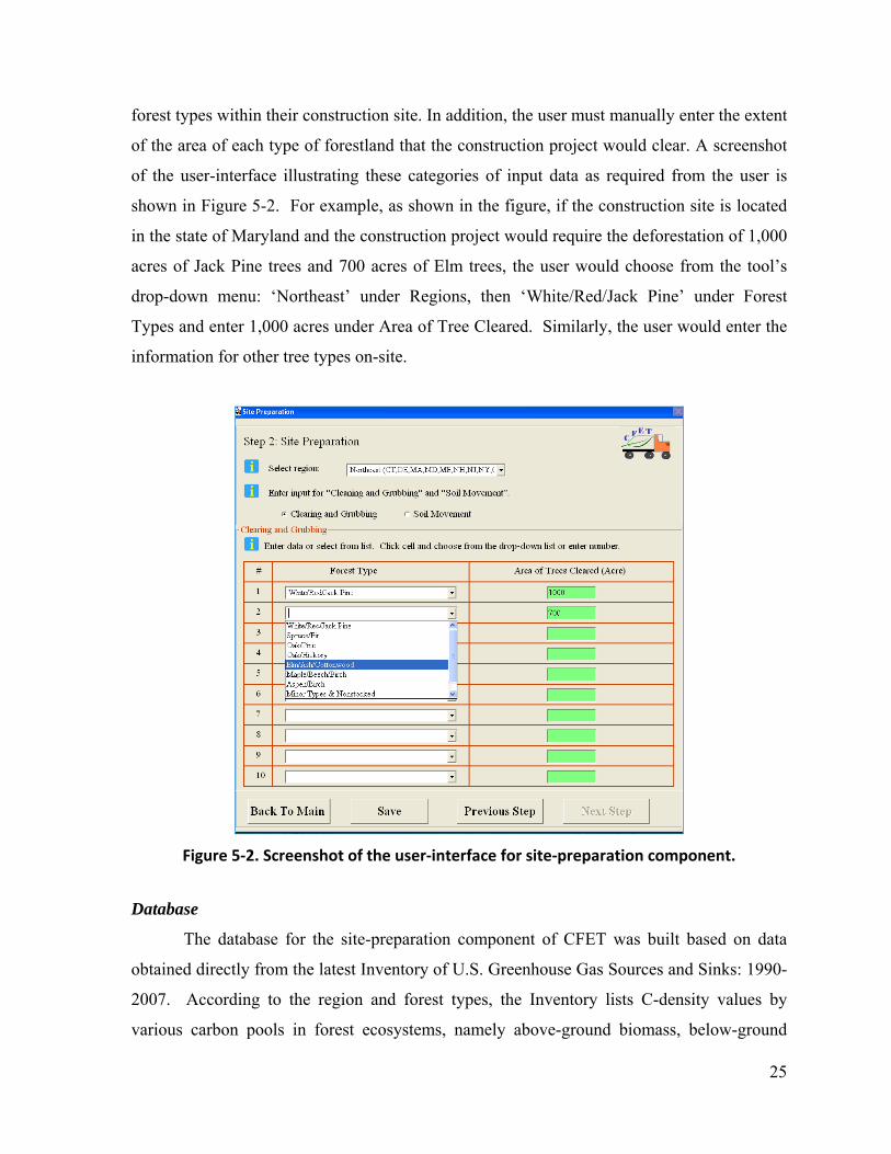
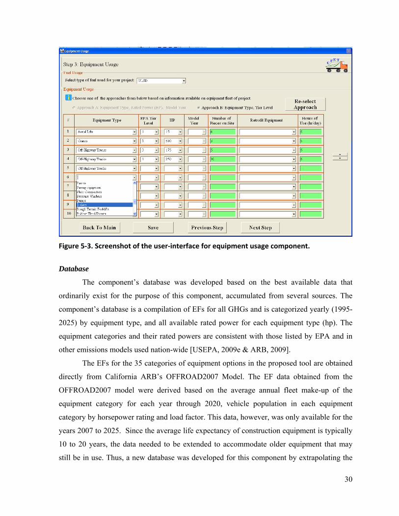
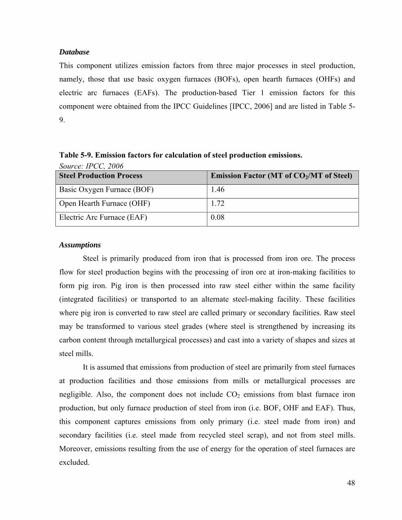
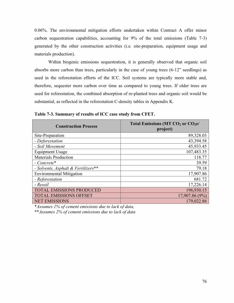
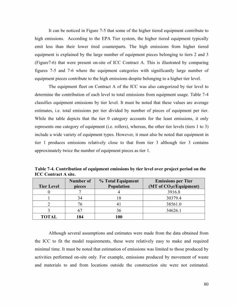
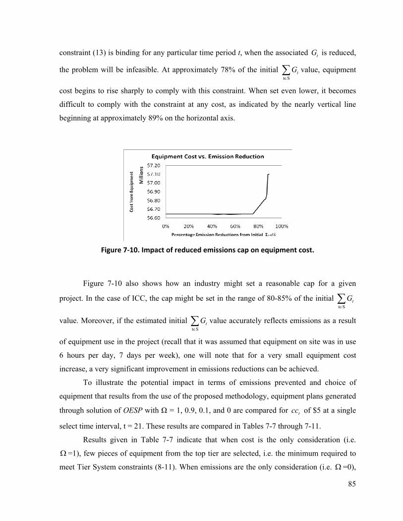
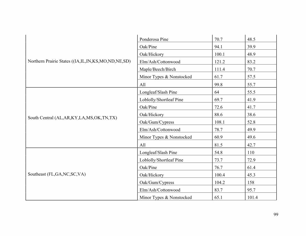
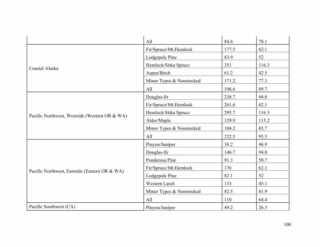
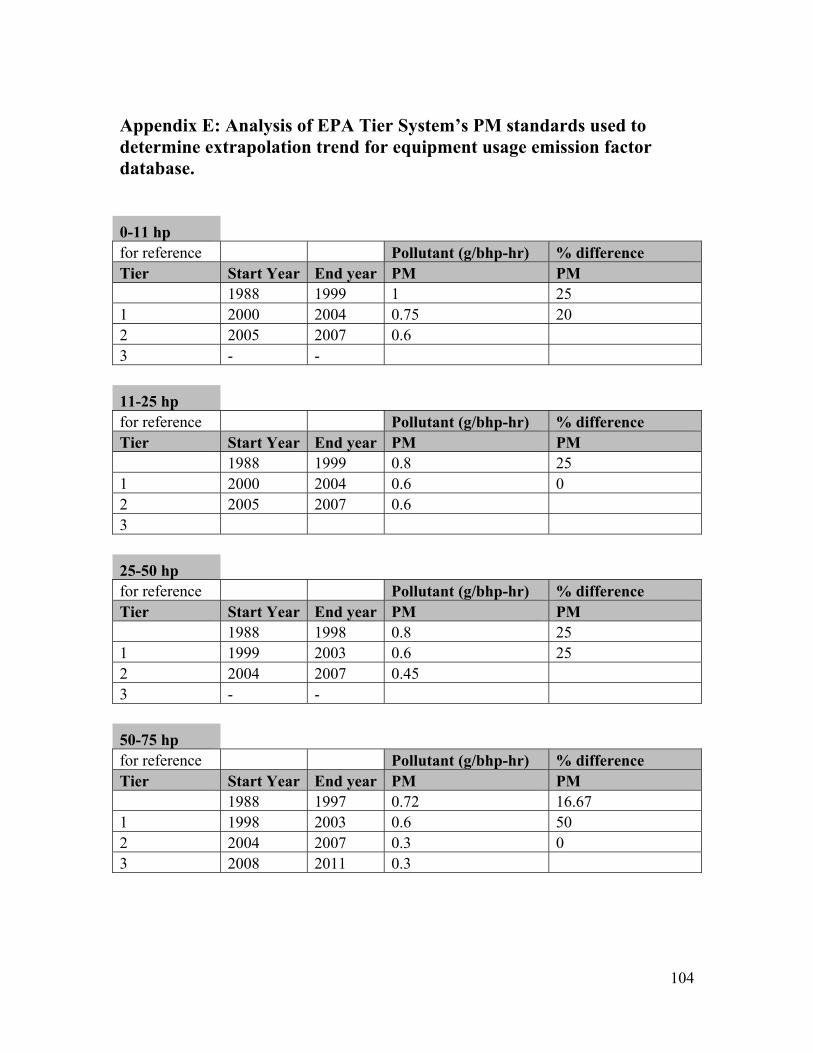
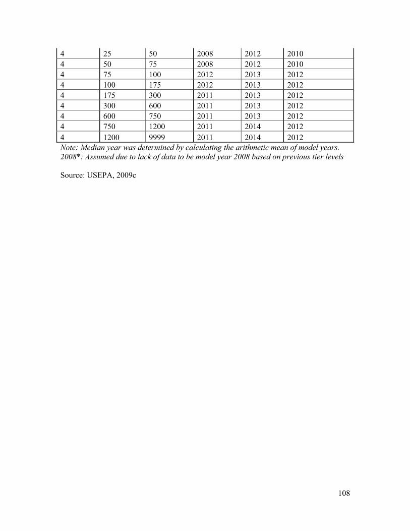
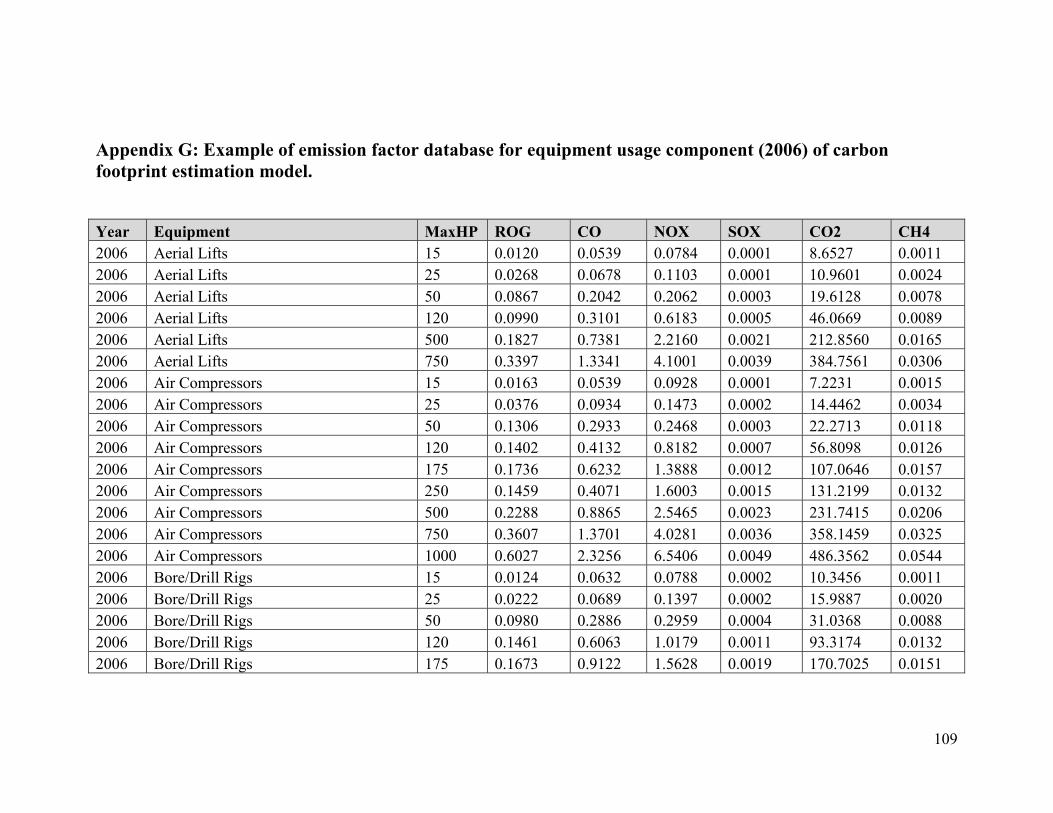
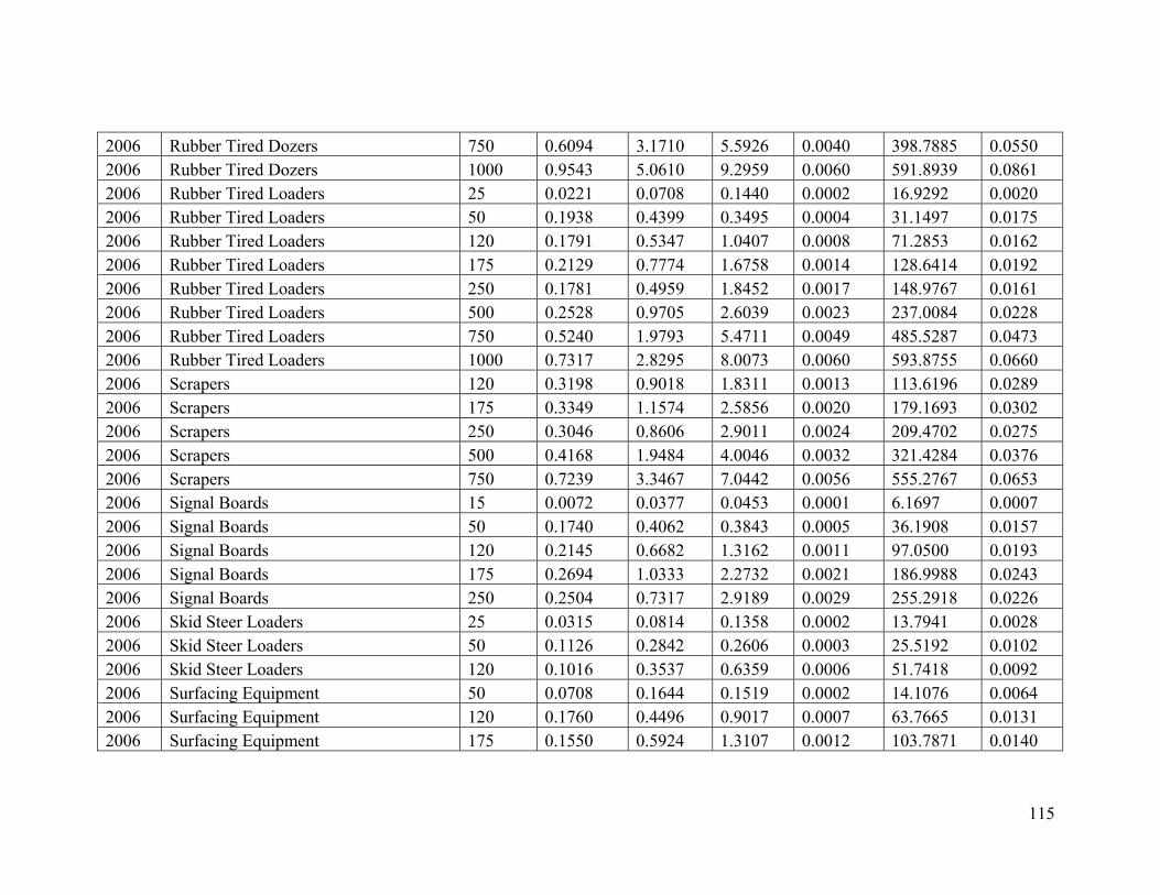
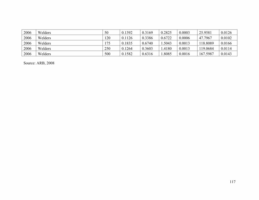
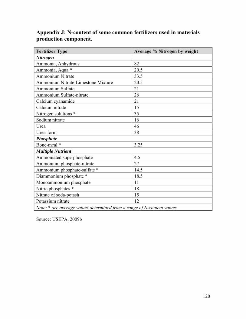
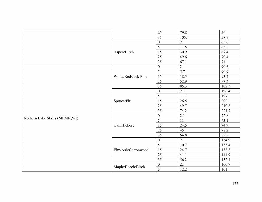
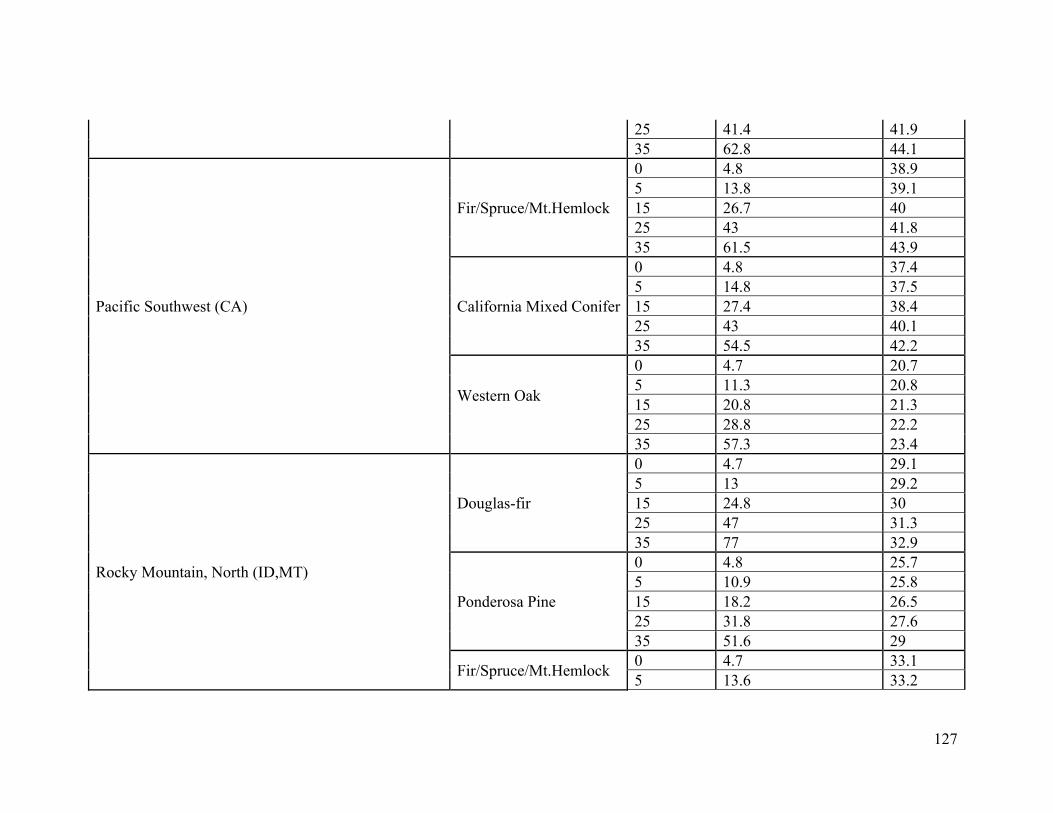
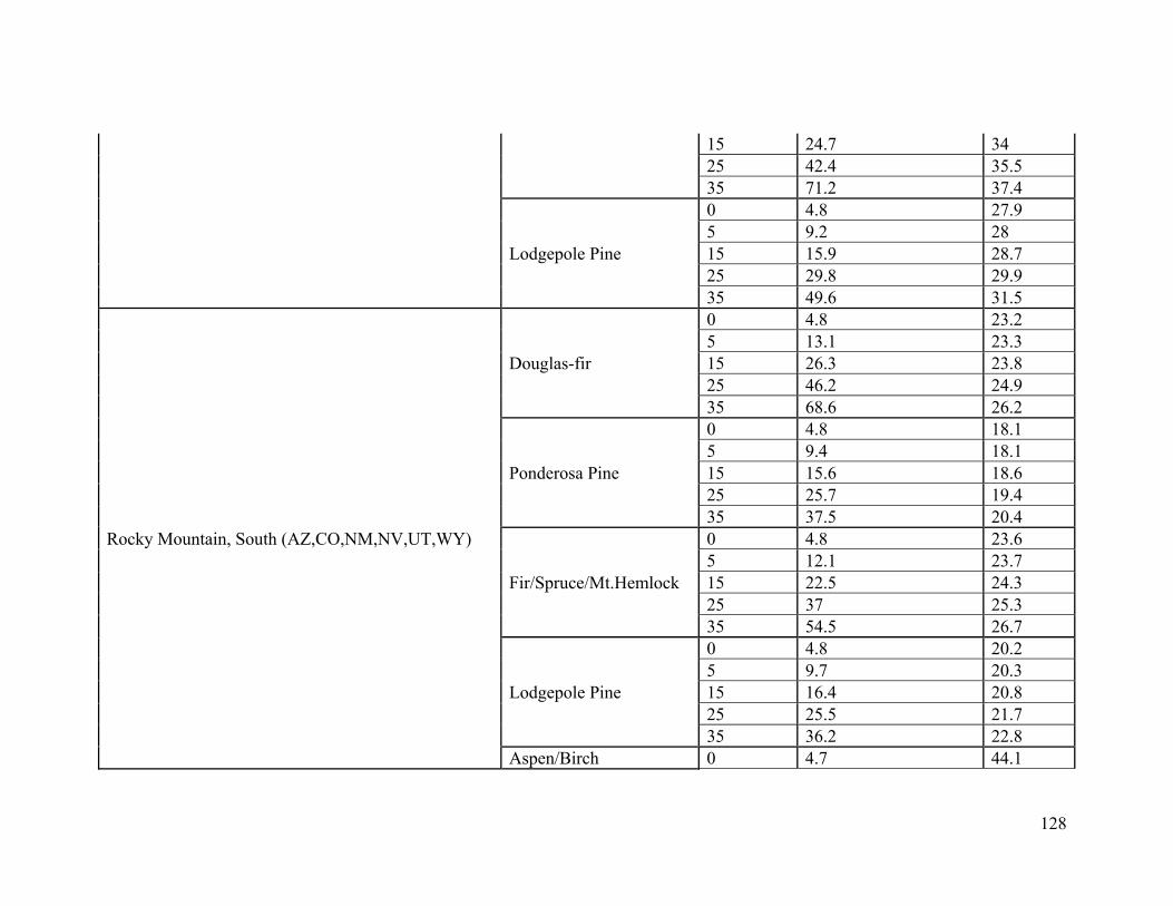
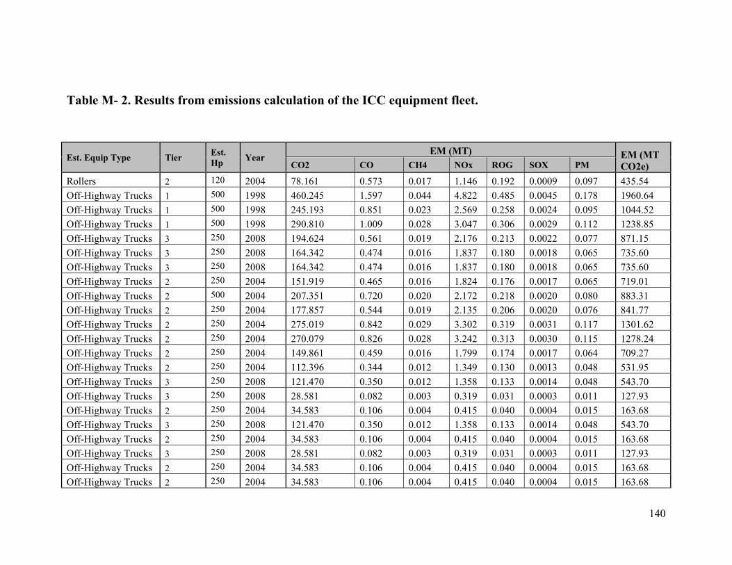
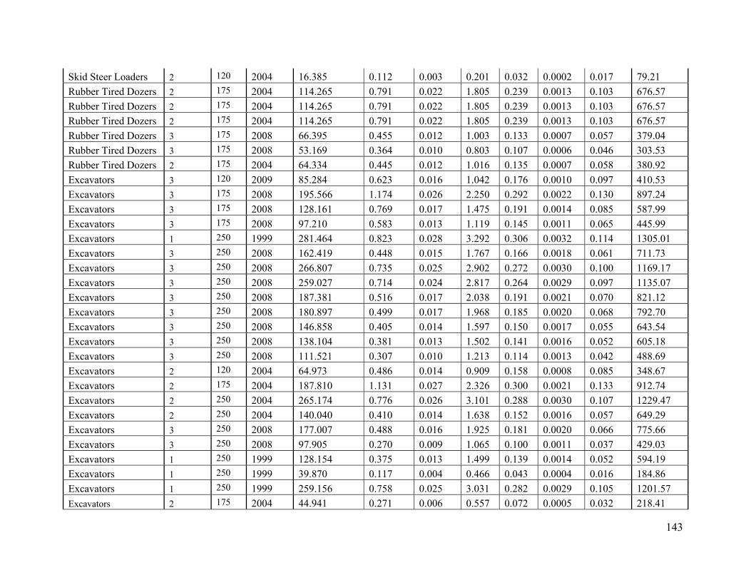
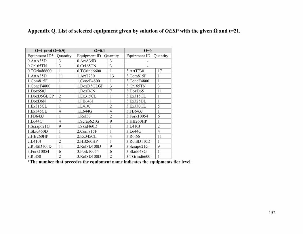
Agriculture. New Orleans, Louisiana. 1994.