55
Topic 28: Unequal Replication in Two- Way ANOVA
| Date post: | 27-Dec-2015 |
| Category: |
Documents |
| Upload: | aleesha-atkinson |
| View: | 233 times |
| Download: | 0 times |
Topic 28: Unequal Replication in Two-Way
ANOVA

Outline
• Two-way ANOVA with unequal numbers of observations in the cells
–Data and model
–Regression approach
–Parameter estimates
• Previous analyses with constant n just special case

Data for two-way ANOVA
• Y is the response variable
• Factor A with levels i = 1 to a
• Factor B with levels j = 1 to b
• Yijk is the kth observation in cell (i,j)
• k = 1 to nij and nij may vary

Recall Bread Example• KNNL p 833• Y is the number of cases of bread sold• A is the height of the shelf display, a=3
levels: bottom, middle, top• B is the width of the shelf display, b=2:
regular, wide• n=2 stores for each of the 3x2
treatment combinations (BALANCED)
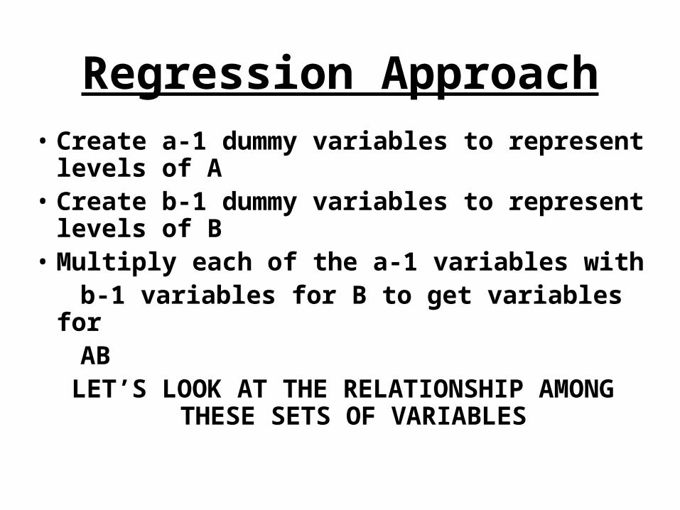
Regression Approach
• Create a-1 dummy variables to represent levels of A
• Create b-1 dummy variables to represent levels of B
• Multiply each of the a-1 variables with b-1 variables for B to get variables for AB
LET’S LOOK AT THE RELATIONSHIP AMONG THESE SETS OF VARIABLES
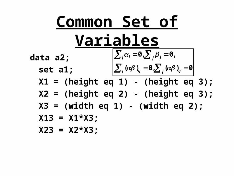
Common Set of Variables
data a2;
set a1;
X1 = (height eq 1) - (height eq 3);
X2 = (height eq 2) - (height eq 3);
X3 = (width eq 1) - (width eq 2);
X13 = X1*X3;
X23 = X2*X3;
j iji ij
j ji i
0)(,0)(
,0,0
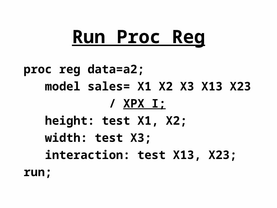
Run Proc Reg
proc reg data=a2;
model sales= X1 X2 X3 X13 X23
/ XPX I;
height: test X1, X2;
width: test X3;
interaction: test X13, X23;
run;

X′X MatrixModel Crossproducts X'X X'Y Y'Y
Variable Intercept X1 X2 X3 X13 X23Intercept 12 0 0 0 0 0
X1 0 8 4 0 0 0
X2 0 4 8 0 0 0
X3 0 0 0 12 0 0
X13 0 0 0 0 8 4
X23 0 0 0 0 4 8
Sets of variables orthogonal
Cross-products between sets is 0
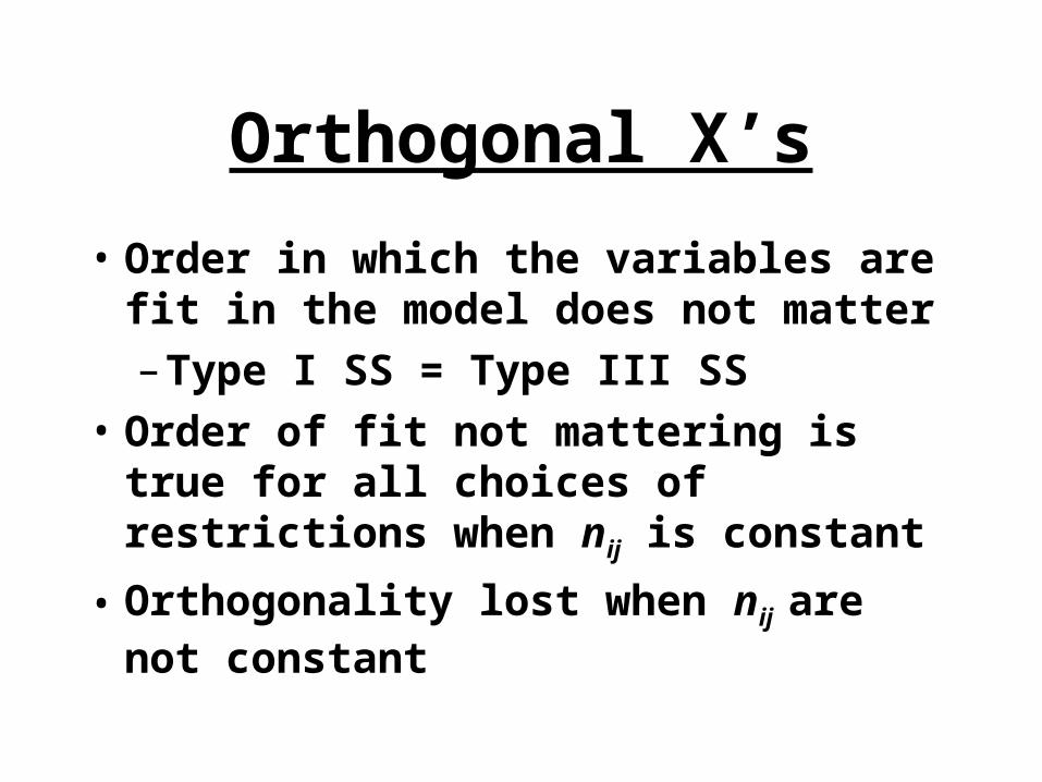
Orthogonal X’s
• Order in which the variables are fit in the model does not matter–Type I SS = Type III SS
• Order of fit not mattering is true for all choices of restrictions when nij is constant
• Orthogonality lost when nij are not constant
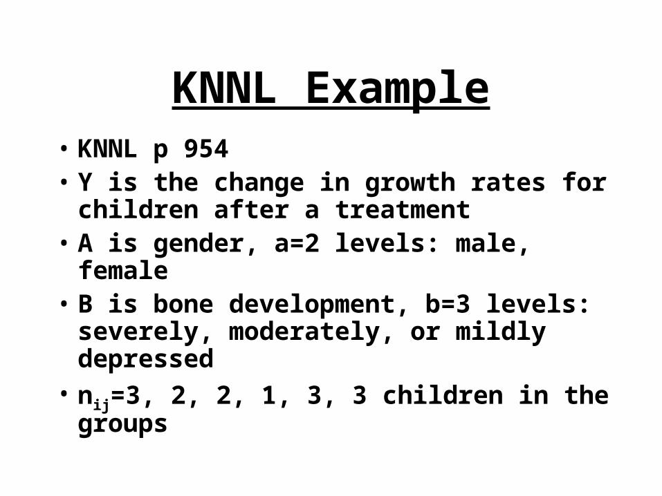
KNNL Example• KNNL p 954• Y is the change in growth rates for
children after a treatment • A is gender, a=2 levels: male, female• B is bone development, b=3 levels:
severely, moderately, or mildly depressed
• nij=3, 2, 2, 1, 3, 3 children in the groups

Read and check the data
data a3; infile 'c:\...\CH23TA01.txt'; input growth gender bone;proc print data=a1; run;
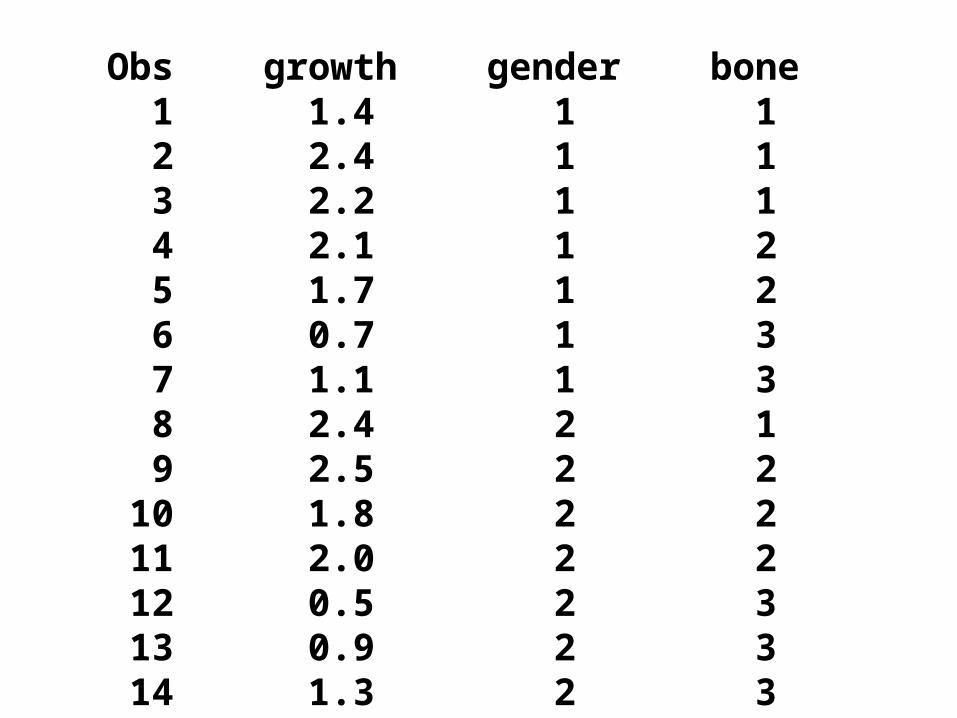
Obs growth gender bone 1 1.4 1 1 2 2.4 1 1 3 2.2 1 1 4 2.1 1 2 5 1.7 1 2 6 0.7 1 3 7 1.1 1 3 8 2.4 2 1 9 2.5 2 2 10 1.8 2 2 11 2.0 2 2 12 0.5 2 3 13 0.9 2 3 14 1.3 2 3

Common Set of Variables
data a3;
set a3;
X1 = (bone eq 1) - (bone eq 3);
X2 = (bone eq 2) - (bone eq 3);
X3 = (gender eq 1) - (gender eq 2);
X13 = X1*X3;
X23 = X2*X3;
j iji ij
j ji i
0)(,0)(
,0,0
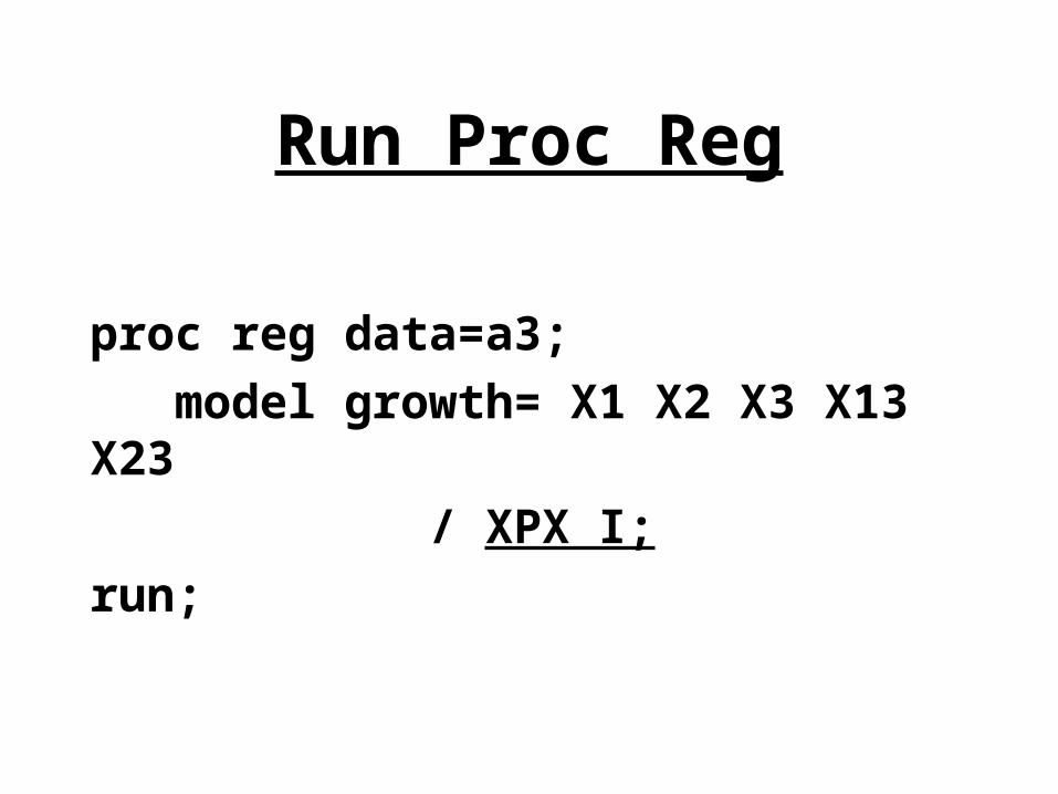
Run Proc Reg
proc reg data=a3;
model growth= X1 X2 X3 X13 X23
/ XPX I;
run;

X′X MatrixModel Crossproducts X'X X'Y Y'Y
Variable Intercept X1 X2 X3 X13 X23Intercept 14 -1 0 0 3 0
X1 -1 9 5 3 1 -1
X2 0 5 10 0 -1 -2
X3 0 3 0 14 -1 0
X13 3 1 -1 -1 9 5
X23 0 -1 -2 0 5 10
Cross-product terms no longer 0
Order of fit matters
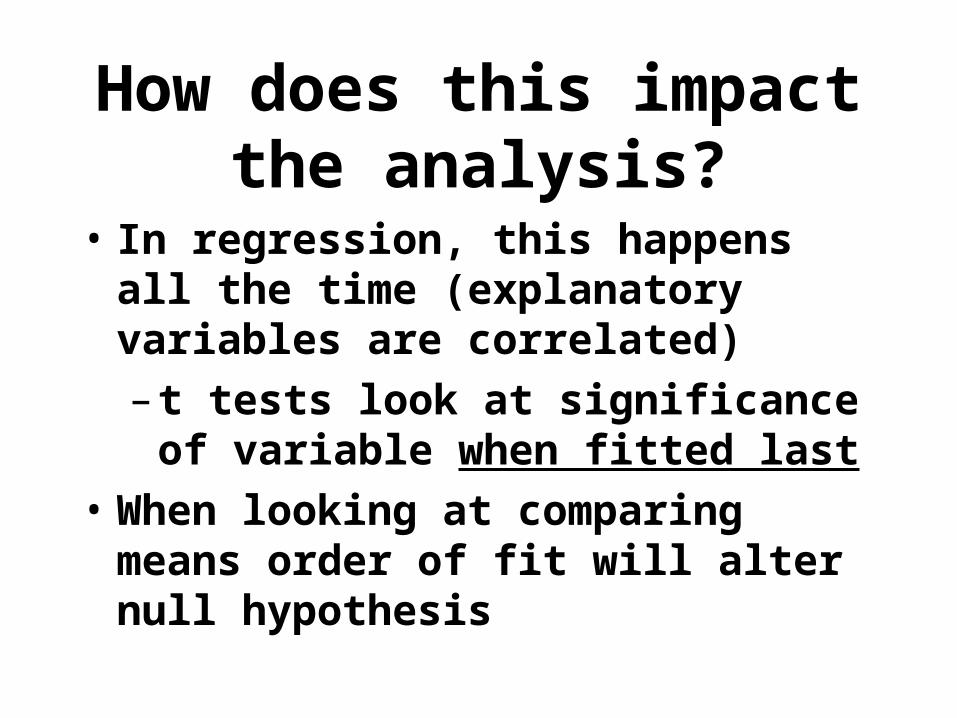
How does this impact the analysis?
• In regression, this happens all the time (explanatory variables are correlated)
– t tests look at significance of variable when fitted last
• When looking at comparing means order of fit will alter null hypothesis
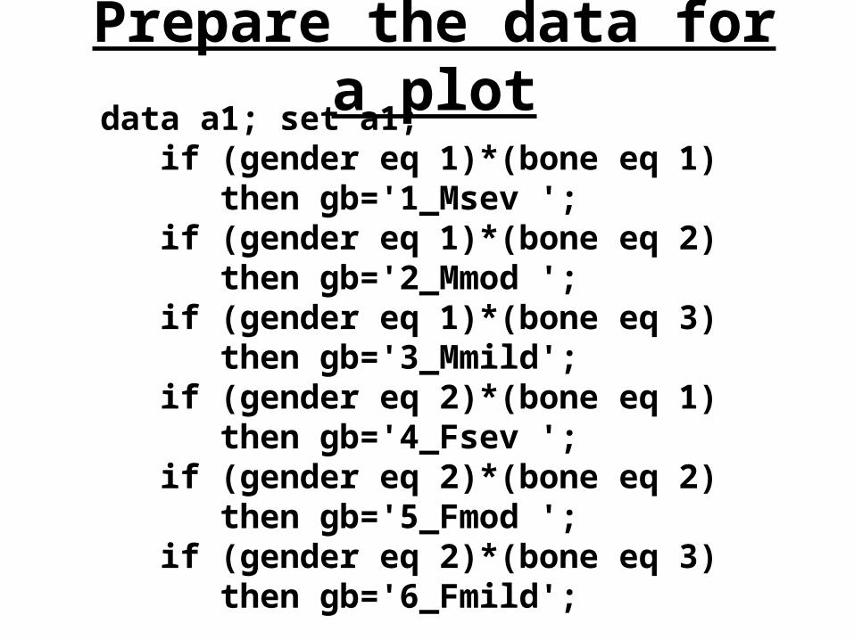
Prepare the data for a plotdata a1; set a1; if (gender eq 1)*(bone eq 1) then gb='1_Msev '; if (gender eq 1)*(bone eq 2) then gb='2_Mmod '; if (gender eq 1)*(bone eq 3) then gb='3_Mmild'; if (gender eq 2)*(bone eq 1) then gb='4_Fsev '; if (gender eq 2)*(bone eq 2) then gb='5_Fmod '; if (gender eq 2)*(bone eq 3) then gb='6_Fmild';

Plot the data
title1 'Plot of the data';symbol1 v=circle i=none;proc gplot data=a1; plot growth*gb;run;

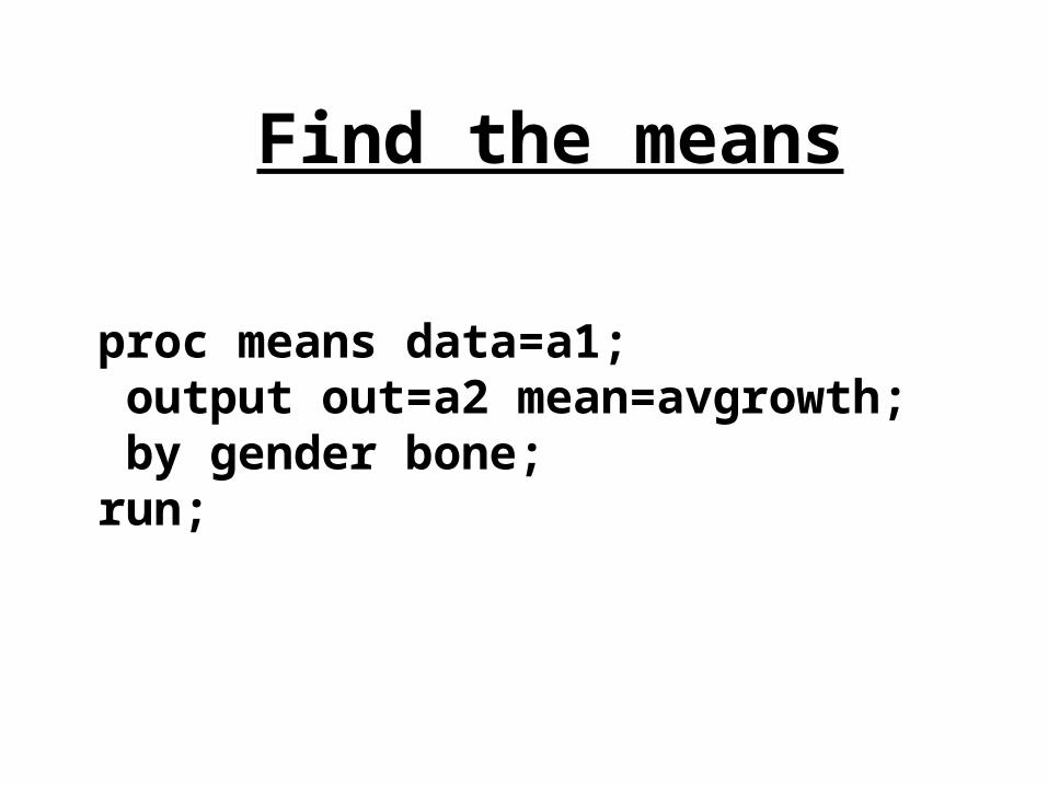
Find the means
proc means data=a1; output out=a2 mean=avgrowth; by gender bone;run;

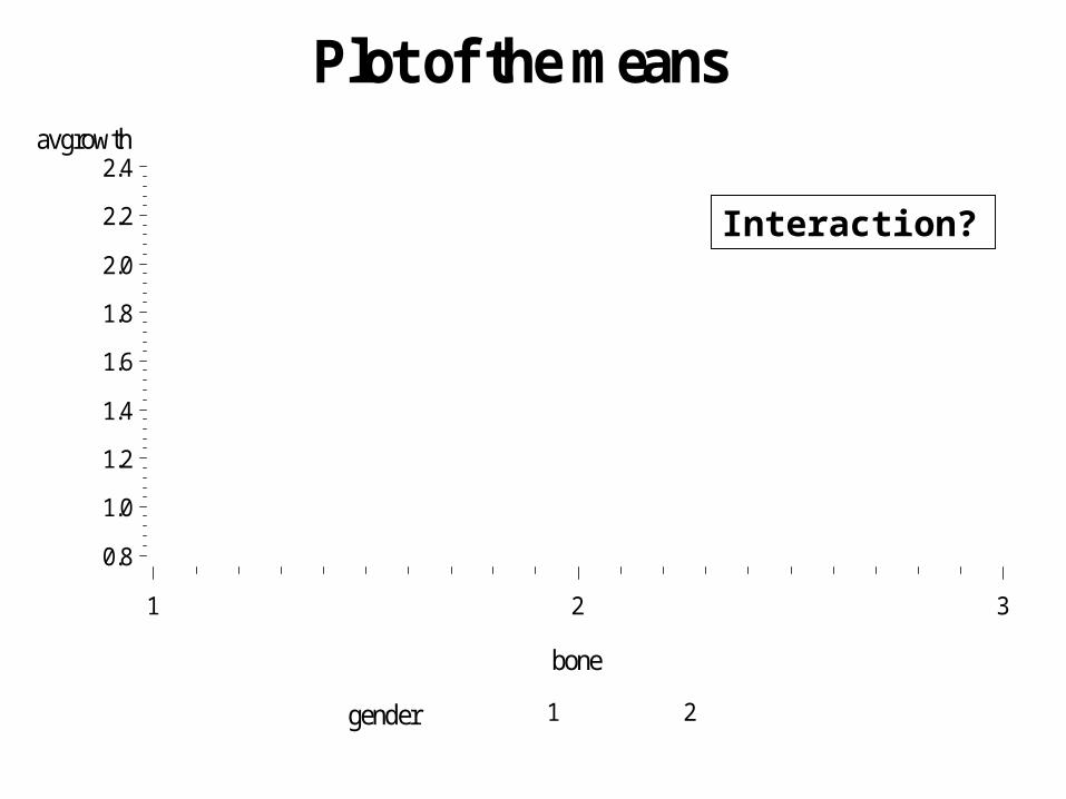
Plot the means
title1 'Plot of the means';symbol1 v='M' i=join c=blue;symbol2 v='F' i=join c=green;proc gplot data=a2; plot avgrowth*bone=gender;run;
avgrowth
0.8
1.0
1.2
1.4
1.6
1.8
2.0
2.2
2.4
bone
1 2 3
Plot of the means
gender 1 2
Interaction?
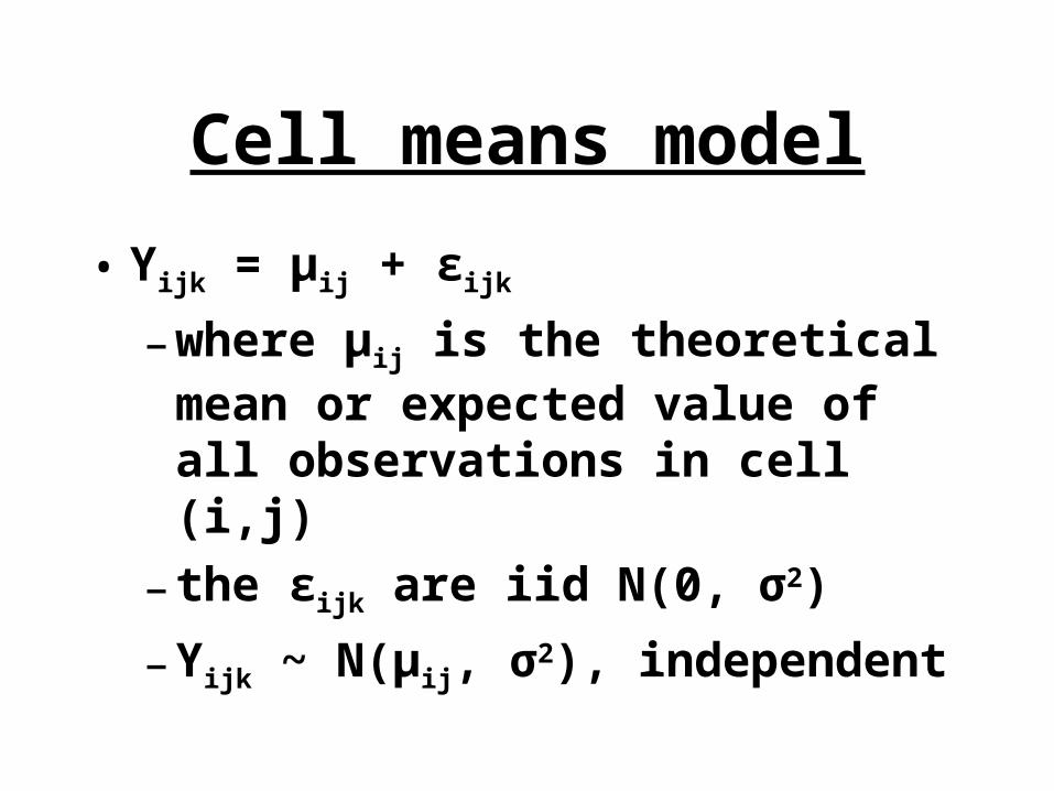
Cell means model
• Yijk = μij + εijk
–where μij is the theoretical mean or expected value of all observations in cell (i,j)
– the εijk are iid N(0, σ2)
–Yijk ~ N(μij, σ2), independent

Estimates
• Estimate μij by the mean of the observations in cell (i,j),
• For each (i,j) combination, we can get an estimate of the variance
• We pool these to get an estimate of σ2
ij.Y
ijn/)Y(Y k ijkij.
k ijij ns )1/()YY( 2ij.ijk
2
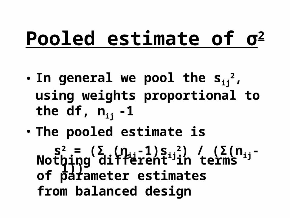
Pooled estimate of σ2
• In general we pool the sij2, using
weights proportional to the df, nij -1
• The pooled estimate is
s2 = (Σ (nij-1)sij2) / (Σ(nij-1))
Nothing different in terms of parameter estimates from balanced design

Run proc glm
proc glm data=a1; class gender bone; model growth=gender|bone/solution; means gender*bone;run;
Shorthand way to write main effects and interactions
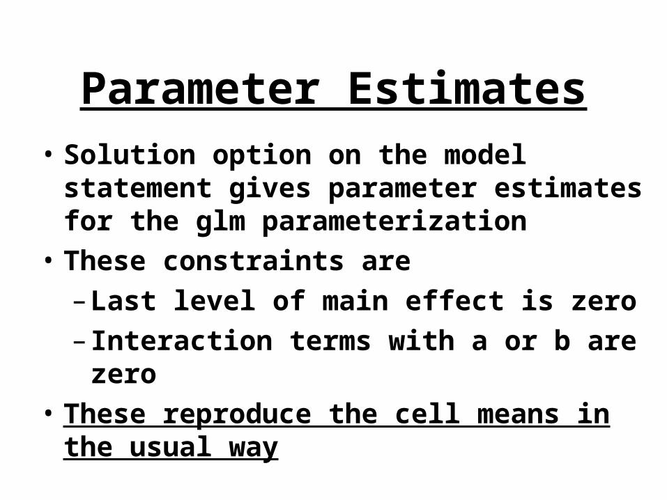
Parameter Estimates• Solution option on the model statement
gives parameter estimates for the glm parameterization
• These constraints are
–Last level of main effect is zero
– Interaction terms with a or b are zero
• These reproduce the cell means in the usual way
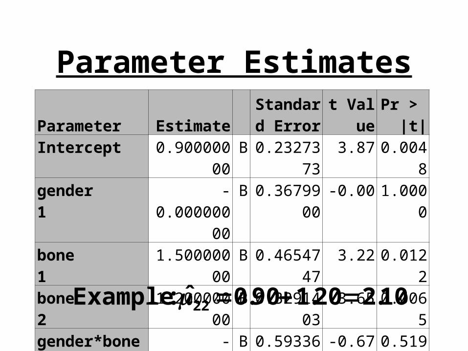
Parameter Estimates
Parameter Estimate Standard
Error t Value Pr > |t|Intercept 0.90000000 B 0.2327373 3.87 0.0048
gender 1 -0.00000000 B 0.3679900 -0.00 1.0000
bone 1 1.50000000 B 0.4654747 3.22 0.0122
bone 2 1.20000000 B 0.3291403 3.65 0.0065
gender*bone 1 1 -0.40000000 B 0.5933661 -0.67 0.5192
gender*bone 1 2 -0.20000000 B 0.5204165 -0.38 0.7108
10.220.190.0ˆ :Example 22

Output
Note DF and SS add as usual
Source DFSum of
SquaresMean
Square F Value Pr > FModel 5 4.4742857 0.89485714 5.51 0.0172Error 8 1.3000000 0.16250000 Corrected Total
13 5.7742857
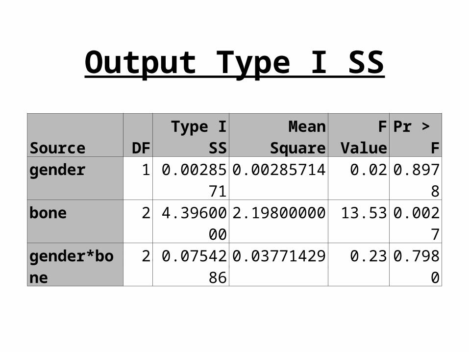
Output Type I SS
SSG+SSB+SSGB=4.47429
Source DF Type I SS Mean Square F Value Pr > Fgender 1 0.0028571 0.00285714 0.02 0.8978
bone 2 4.3960000 2.19800000 13.53 0.0027
gender*bone 2 0.0754286 0.03771429 0.23 0.7980

Output Type III SS
SSG+SSB+SSGB=4.38514
Source DF Type III SS Mean Square F Value Pr > Fgender 1 0.12000000 0.12000000 0.74 0.4152
bone 2 4.18971429 2.09485714 12.89 0.0031
gender*bone 2 0.07542857 0.03771429 0.23 0.7980

Type I vs Type III
• SS for Type I add up to model SS
• SS for Type III do not necessarily add up
• Type I and Type III are the same for the interaction because last term in model
• The Type I and Type III analysis for the main effects are not necessarily the same
• Different hypotheses are being examined
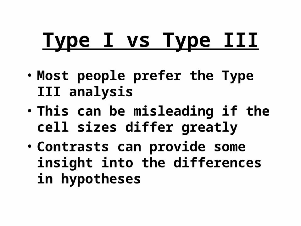
Type I vs Type III
• Most people prefer the Type III analysis
• This can be misleading if the cell sizes differ greatly
• Contrasts can provide some insight into the differences in hypotheses
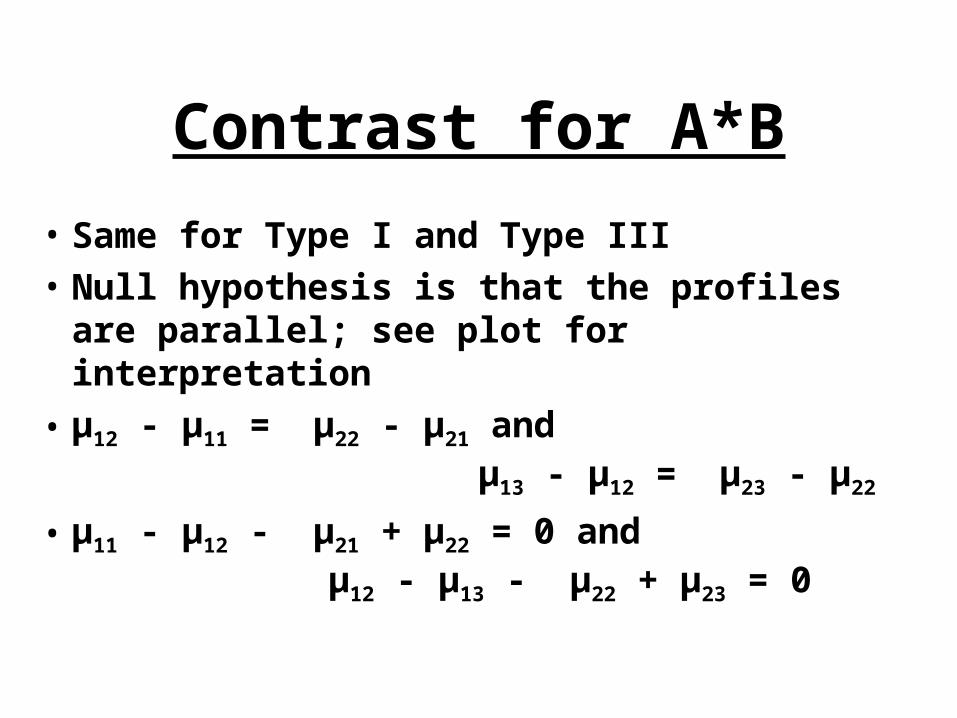
Contrast for A*B
• Same for Type I and Type III
• Null hypothesis is that the profiles are parallel; see plot for interpretation
• μ12 - μ11 = μ22 - μ21 and μ13 - μ12 = μ23 - μ22
• μ11 - μ12 - μ21 + μ22 = 0 and μ12 - μ13 - μ22 + μ23 = 0
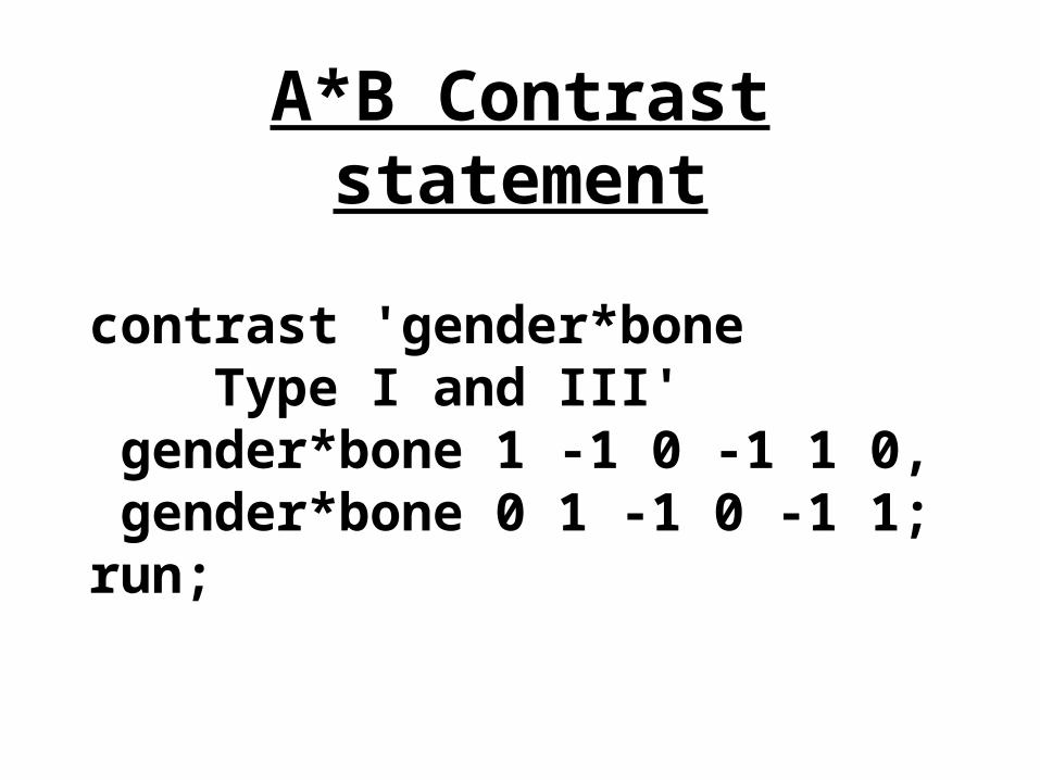
A*B Contrast statement
contrast 'gender*bone Type I and III' gender*bone 1 -1 0 -1 1 0, gender*bone 0 1 -1 0 -1 1;run;

Type III Contrast for gender
• (1) μ11 = (1)(μ + α1 + β1 + (αβ)11)
• (1) μ12 = (1)(μ + α1 + β2 + (αβ)12)
• (1) μ13 = (1)(μ + α1 + β3 + (αβ)13)
• (-1) μ21 = (-1)(μ + α2 + β1 + (αβ)21)
• (-1) μ22 = (-1)(μ + α2 + β2 + (αβ)22)
• (-1) μ23 = (-1)(μ + α2 + β3 + (αβ)23)
L = 3α1 – 3α2 + (αβ)11 + (αβ)12 + (αβ)13 – (αβ)21
– (αβ)22 – αβ23

Contrast statementGender Type III
contrast 'gender Type III' gender 3 -3 gender*bone 1 1 1 -1 -1 -1;
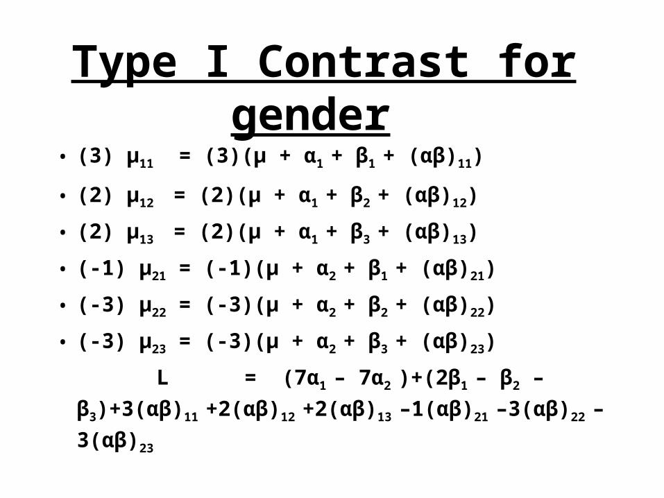
Type I Contrast for gender
• (3) μ11 = (3)(μ + α1 + β1 + (αβ)11)
• (2) μ12 = (2)(μ + α1 + β2 + (αβ)12)
• (2) μ13 = (2)(μ + α1 + β3 + (αβ)13)
• (-1) μ21 = (-1)(μ + α2 + β1 + (αβ)21)
• (-3) μ22 = (-3)(μ + α2 + β2 + (αβ)22)
• (-3) μ23 = (-3)(μ + α2 + β3 + (αβ)23)
L = (7α1 – 7α2 )+(2β1 – β2 – β3)+3(αβ)11
+2(αβ)12 +2(αβ)13 –1(αβ)21 –3(αβ)22 –3(αβ)23
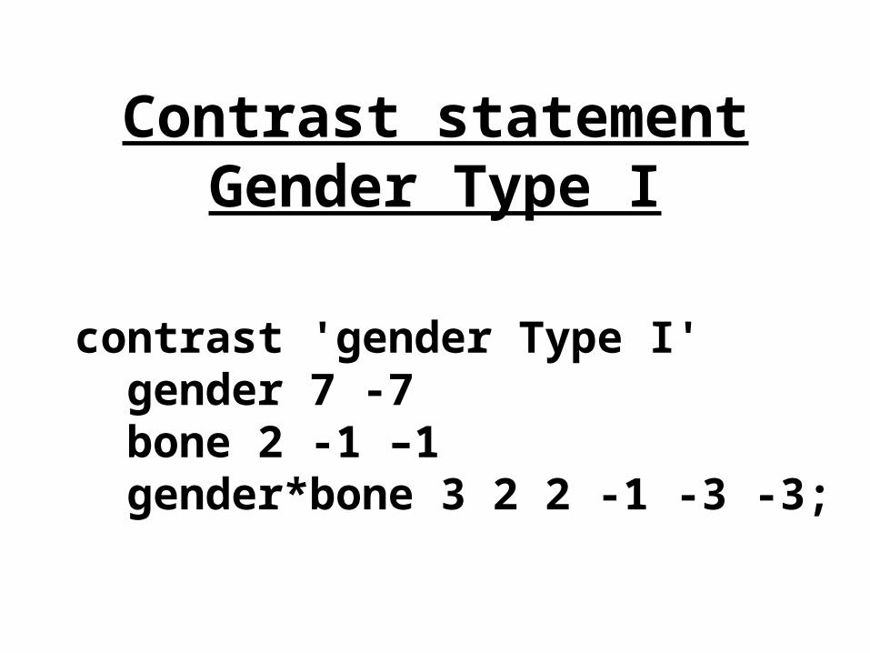
Contrast statementGender Type I
contrast 'gender Type I' gender 7 -7 bone 2 -1 –1 gender*bone 3 2 2 -1 -3 -3;

Contrast output
Contrast DF Contrast SSgender Type III 1 0.12000000gender Type I 1 0.00285714 bone Type III 2 4.18971429gender*bone Type I and III 2 0.07542857

Summary
• Type I and Type III F tests test different null hypotheses
• Should be aware of the differences
• Most prefer Type III as it follows logic similar to regression analysis
• Be wary, however, if the cell sizes vary dramatically
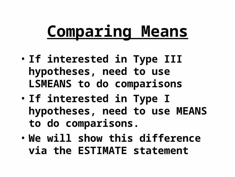
Comparing Means
• If interested in Type III hypotheses, need to use LSMEANS to do comparisons
• If interested in Type I hypotheses, need to use MEANS to do comparisons.
• We will show this difference via the ESTIMATE statement

SAS Commands
• Will use earlier contrast code to set up the ESTIMATE commands
estimate 'gender Type III' gender 3 -3
gender*bone 1 1 1 -1 -1 -1 / divisor=3;
estimate 'gender Type I' gender 7 -7
bone 2 -1 -1 gender*bone 3 2 2 -1 -3 -3 /
divisor=7;

MEANS OUPUT
Level of ------------growth-----------gender N Mean Std Dev
1 7 1.65714286 0.624118432 7 1.62857143 0.75655862
Diff = 0.0286

LSMEANS OUPUT
growthgender LSMEAN
1 1.600000002 1.80000000
Diff = -0.20

Estimate output
Parameter Estimate Std Errgender Type III -0.200 0.2327gender Type I 0.029 0.2155
Notice that these two estimates agree with the difference of estimates for LSMEANS or MEANS

Analytical Strategy
• First examine interaction• Some options when the interaction is
significant– Interpret the plot of means–Run A at each level of B and/or B
at each level of A–Run as a one-way with ab levels–Use contrasts
Analytical Strategy
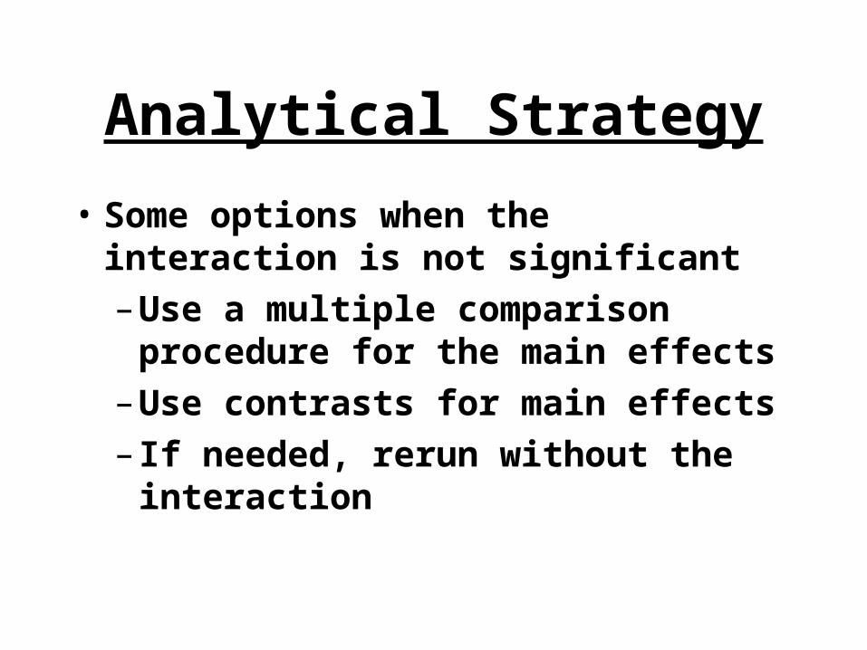
• Some options when the interaction is not significant
–Use a multiple comparison procedure for the main effects
–Use contrasts for main effects
– If needed, rerun without the interaction

Example continued
proc glm data=a3; class gender bone; model growth=gender bone/ solution; means gender bone/ tukey lines;run;
Pool here because small df error
For Type I hypotheses
Output
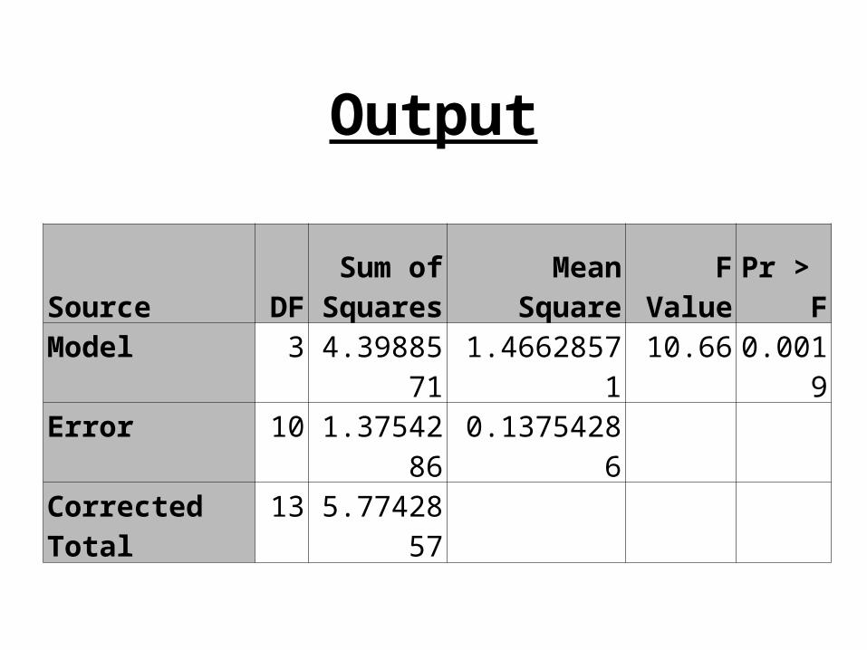
Source DFSum of
Squares Mean Square F Value Pr > FModel 3 4.3988571 1.46628571 10.66 0.0019
Error 10 1.3754286 0.13754286
Corrected Total 13 5.7742857

Output Type I SS
Source DF Type I SS Mean Square F Value Pr > Fgender 1 0.00285714 0.00285714 0.02 0.8883
bone 2 4.39600000 2.19800000 15.98 0.0008
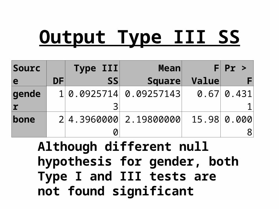
Output Type III SS
Source DF Type III SS Mean Square F Value Pr > Fgender 1 0.09257143 0.09257143 0.67 0.4311
bone 2 4.39600000 2.19800000 15.98 0.0008
Although different null hypothesis for gender, both Type I and III tests are not found significant
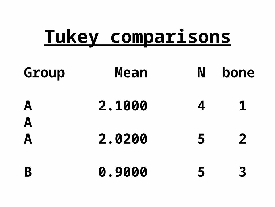
Tukey comparisons
Group Mean N bone
A 2.1000 4 1AA 2.0200 5 2
B 0.9000 5 3
Tukey Comparisons
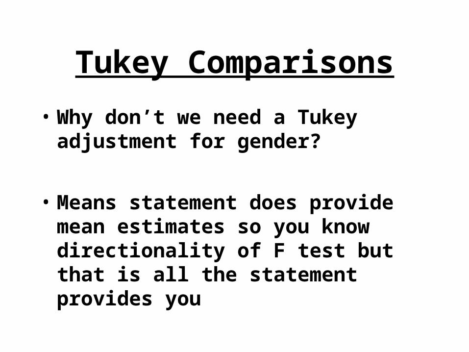
• Why don’t we need a Tukey adjustment for gender?
• Means statement does provide mean estimates so you know directionality of F test but that is all the statement provides you

Last slide
• Read KNNL Chapter 23
• We used program topic28.sas to generate the output for today


