155
Prepared by: V M Naidu; GAYATRI VIDYA PARISHAD COLLEGE OF ENGINNERING TRANSPORTATION ENGINEERING-I GVPCE(A) B.Tech (Civil Engineering, V Semester)

Prepared by: V M Naidu; GAYATRI VIDYA PARISHAD COLLEGE OF ENGINNERING
TRANSPORTATION ENGINEERING-I
GVPCE(A)
B.Tech (Civil Engineering, V Semester)
Prepared by: V M Naidu; GAYATRI VIDYA PARISHAD COLLEGE OF ENGINNERING
UNIT:-1
HIGHWAY DEVELOPMENT AND PLANNING
HIGHWAY DEVELOPMENT IN INDIA:
VARIOUS STAGES:
1. Roads in ancient India.
2. Roads in Mughal period.
3. Roads in nineteenth century.
ROAD DEVELOPMENT PLANS:
4. Jayakar committee and recommendations (1927)
• Introduced central road fund, IRC, Motor vehicle act.
5. Nagpur conference (1943)
• Formed CRRI, National highway act.
6. Second 20 yr road development plan (1961-81)
• Formed Highway research board.
7. National transport policy committee.
8. Third 20yr road development plan (1981-2001)
NECCESITY OF HIGHWAY PLANNING:
Objectives:
1. To plan a road network for efficient and safe traffic operation.
2. To arrive maximum utility.
Prepared by: V M Naidu; GAYATRI VIDYA PARISHAD COLLEGE OF ENGINNERING
3. To fix date wise priorities development.
4. To plan for future requirements and improvements.
5. To work out financing system.
CLASSIFICATION OF ROADS:
1. Based on usage during different seasons.
• All weather roads
• Fair weather roads
2. Based on type of carriage way.
• Paved roads (eg: bitumen, concrete roads)
• Unpaved roads (eg: earthen, gravel roads)
3. Based on pavement surfacing.
• Surfaced roads
• Unsurfaced roads
CLASSIFICATION OF ROADS BY NAGPUR ROAD PLAN:
1. National highways.
• Connects major ports, capitals of larger states, larger industrial and
tourist centres.
• Constructed by centre.
Eg: NH-1: Delhi-Ambala-Amritsar
NH-2: Mumbai-Agra
2. State Highways.
• Connects district head quarters and important cities.
• NH, SH are designed for same speeds.
3. Major district roads.
• Connects production centres and markets.
• Its speeds are lower than NH, SH.
4. Other district roads.

Prepared by: V M Naidu; GAYATRI VIDYA PARISHAD COLLEGE OF ENGINNERING
• Connects market centres, taluk head quarters.
• Lower design specifications than MDR.
5. Village roads.
• Connects villages and group of villages.
MODIFIED CLASSIFICATIN BASEDE ON THIERD ROAD DEVELOPMENT PLAN:
1. Primary system.
• Express ways.
• National highways (NH).
2. Secondary system.
• State highways (SH).
• Major district roads (MDR).
3. Tertiary system.
• Other district roads (ODR).
• Village roads (VR).
Classification of urban roads:-
• Arterial.
• Sub-arterial.
• Collector streets.
• Local streets.
ROAD PATTERNS:
a. Rectangular or Block pattern.

Prepared by: V M Naidu; GAYATRI VIDYA PARISHAD COLLEGE OF ENGINNERING
b. Radial or Star and Block pattern.
c. Radial or Star Circular pattern.
d. Radial or star and grid pattern.

Prepared by: V M Naidu; GAYATRI VIDYA PARISHAD COLLEGE OF ENGINNERING
e. Hexagonal pattern.
f. Minimum travel pattern
HIGHWAY ALIGNMENT:
Definition: The position or layout of the centre line of the highway line on the
ground is called the alignment.
• Horizontal alignment includes straight path, horizontal deviations and
curves.
• Vertical alignment includes gradients, vertical curves.
Improper alignment leads to
• Increase in construction cost.
• Increase in maintenance cost.
• Increase in vehicle operation rate.
• Increase in accident rate.
REQUIREMENTS OF ALIGNMENT:
Prepared by: V M Naidu; GAYATRI VIDYA PARISHAD COLLEGE OF ENGINNERING
• Short
• Easy
• Safe
• Economical
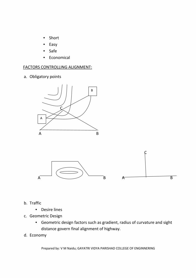
FACTORS CONTROLLING ALIGNMENT:
a. Obligatory points
C
A B
C
A B A B
b. Traffic
• Desire lines
c. Geometric Design
• Geometric design factors such as gradient, radius of curvature and sight
distance govern final alignment of highway.
d. Economy
A
B

Prepared by: V M Naidu; GAYATRI VIDYA PARISHAD COLLEGE OF ENGINNERING
• Finalized alignment should be economical.
e. Other considerations
• Various other factors governs alignment are drainage considerations,
hydrological factors and political considerations.
SPECIAL CONSIDERATIONS FOR HILLY AREAS
a) Stability
b) Drainage
c) Geometric standard of hill roads
ENGINEERING SURVEYS
a) Map study
-maps are available from survey of India.
• Alignment avoiding valleys, ponds or lakes.
• When the road has to cross a row of hills.
• Approximate location of bridge will be decided.
b) Reconnaissance
-details to be collected
• Valleys, ponds and lakes.
• Approximate values of gradient, length of gradient and radius of
curvature.
• Number and type of cross drainage structures.
• Soil type along the routes.
• Sources of construction material, water.
c) Preliminary survey
Main objectives,

Prepared by: V M Naidu; GAYATRI VIDYA PARISHAD COLLEGE OF ENGINNERING
• To survey the various alternative alignments.
• To compare different proposals.
• To estimate quantity of earthwork materials.
• To finalize best alignment.
Surveys
1.) Preliminary traverse
2.) Topographical features
3.) Leveling work
4.) Drainage studies and hydrological data
5.) Soil survey
6.) Material survey
7.) Traffic survey
8.) Determination of final centre line
d.) Final location and detailed survey
DRAWINGS AND REPORT:
Drawings
• Key map
• Index map
• Preliminary survey plans
• Detailed plan and longitudinal section
• Detailed cross section
• Land acquisition plan
• Drawings of cross drainage
• Drawings of road intersection
• Land plan showing quarries
PROJECT REPORTS:
• General details of project
• Features of road
Prepared by: V M Naidu; GAYATRI VIDYA PARISHAD COLLEGE OF ENGINNERING
• Road design and specification
• Drainage facilities and cross drainage structure
• Material, labour and equipment
• Rates
• Construction programming
• miscellaneous
UNIT:-2
HIGHWAY MATERIALS
Highway materials:
• Bitumen
• Aggregate
• Soil
Soil is an integral part of the road pavement structure and it provides support
to pavement from beneath
CHARACTERISTICS OF SOIL:
It is mainly of mineral matter formed by disintegration of rocks by action of
water, frost, temperature and pressure
Based on grain size, soil is classified into
• Gravel
• Sand
• Silt
• Clay

Prepared by: V M Naidu; GAYATRI VIDYA PARISHAD COLLEGE OF ENGINNERING
DESIRABLE PROPERTIES OF SOIL:
• Stability
• Incompressibility
• Strength
• Minimum changes in volume
• Good drainage
• Easy of compaction
FACTORS AFFECTING SOIL STRENGTH
• Soil type
• Moisture content
• Dry density
• Internal structure of soil
• Type and mode of stress application
EVALUATION OF SOIL STRENGTHS
Tests are broadly divided into 3 groups
1) Shear tests
• It is carried out on relatively small soil sample in laboratory.
• No of samples need to be collected from different locations.
• Some of the shear tests are direct shear test, tri-axial compression
test, vane shear test etc.,
2) Bearing tests
• These are loading tests carried out on sub-grade soils in-situ with load
bearing area.
Eg:- plate bearing test
3) Penetration tests
• These are small scale bearing tests in which the size of the located area
is relatively much smaller. Penetration / size of loaded area > Penetration / size of loaded area
Prepared by: V M Naidu; GAYATRI VIDYA PARISHAD COLLEGE OF ENGINNERING
Penetration tests bearing tests
Eg:- California Bearing ratio test, cone penetration test
CBR test
CALIFORNIA BEARING RATIO TEST:
- It is developed by 12alifornia division of highways
- Penetration rate 1.25mm/min
- Local values are recorded at 2.5mm and 5.0mm
- Load values are noted of 0.0,0.5,1.0,1.5,2.0,2.5,3,4,5,7.5,10.0 and
12.5mm

Prepared by: V M Naidu; GAYATRI VIDYA PARISHAD COLLEGE OF ENGINNERING
CBR TEST
Load
5.0cm
2.5cm
Penetration (mm)

Prepared by: V M Naidu; GAYATRI VIDYA PARISHAD COLLEGE OF ENGINNERING
CBR % = load sustained by the specimen at 2.5 and 5.0mm
Load sustained by standard aggregate at
Corresponding penetration (1370kg at 2.5mm,
2055kg at 5.0mm)
STONE AGGREGATES:
- These form the major portion of pavement structure and prime
material in pavement structure.
- Aggregate have to bear stresses occuring due to wheel loads.
- It also have to resist wear due to abrasive action of traffic
- These are used in pavement construction in cement concrete,
bituminous concrete and other bituminous constructions.
- Properties of aggregate depends on properties of constitute
material and nature of bond between them.
Aggregates
• Igneous
• Sedimentary
• Metamorphic
-Aggregates are specified based on grain size, shape, texture, and
gradation.
DESIRABLE PROPERTIES OF ROAD AGGREGATE:
1) STRENGTH

Prepared by: V M Naidu; GAYATRI VIDYA PARISHAD COLLEGE OF ENGINNERING
• Aggregate should be sufficiently strong to withstand stresses
due to traffic wheel load.
• It should resist wear and tear and to crushing
2) HARDNESS
• The aggregates used in surface course are subjected to
constant rubbing or abrasion due to moving traffic.
• Abrasion is the rubbing of stones with other materials.
• Attrition is the mutual rubbing of stones.
3) TOUGHNESS:
• Aggregates are in the pavement are subjected to impact due to
moving wheel loads. This resistance to impact is called toughness.
4) DURABILITY:
• The stone used in pavement construction should be durable and
should resist disintegration due to action of weather.
• The property of the stones to withstand the adverse action os
weather called soundness.
5) SHAPE OF AGGREGATES:-
Aggregates:
1) Rounded
2) Cubical
3) Angular or Flaky
4) Elongated
- Angular flaky and elongated particles will have less strength and
durability compared with other
- Rounded aggregates are preferred than other due to low specific area.

Prepared by: V M Naidu; GAYATRI VIDYA PARISHAD COLLEGE OF ENGINNERING
6) ADHESION WITH BITUMEN:
• Aggregates should have less affinity to water than bitumen.
Otherwise bituminous coating on aggregate will be stripped off.
TESTS FOR ROAD AGGREGATE:-
- Tests are required to know the suitability of aggregate for road
construction. The following are the tests for aggregate.
a) Crushing test
b) Abrasion test
c) Impact test
d) Soundness
e) Shape test
f) Specific gravity and water absorption test
g) Bitumen adhesion test
a) AGGREGATE CRUSHING TEST:-
• Strength is assessed by this test.
• Aggregate crushing value provides relative measure of resistance
to crushing under gradually applied compressive load.
• Low crushing value is preferred for construction.
Apparatus for standard test are:
Steel cylinder 15.2cm diameter with a base plate &plunger,
compression testing machine, cylinder measure of diameter
11.5cm and height 18cm, tamping rods and sieves.

Prepared by: V M Naidu; GAYATRI VIDYA PARISHAD COLLEGE OF ENGINNERING
CRUSHING TEST APPARATUS
11.5d 1 111111 18cm 45-60cm
11.5cm
Cylindrical measure Steel tamping rod
1) Aggregate size <12.5mm&>10mm is taken.
110-
115cm
13-
14cm
15cm

Prepared by: V M Naidu; GAYATRI VIDYA PARISHAD COLLEGE OF ENGINNERING
2) Aggregate filled in cylinder measure in 3 layers, each layer is
ramped with 25 times by tamping rod.
3) The weighed, w1 (g) and placed in test cylinder in 3 layers
with 25 blows each time.
4) Load is applied through plunger (40tonnes) at rate of
4tonnes/min by compression machine.
5) The crushed aggregate is sieved on 2.36mm sieve
6) The crushed material which passed through 2.36mm are
weighed (w2 g).
Aggregate crushing value = w2/w1*100
For Base course <= 45%
Surface course <=30%.
b) ABRASION TESTS:-
• Due to movement of traffic, the road stones in the surface
course are subjected to wearing action.
• Road stones should be hard enough to resist abrasion
action.
Abrasion test can be carried out by following 3 tests:
1) Los angeles abrasion test
2) Deval abrasion test
3) Dorry abrasion test
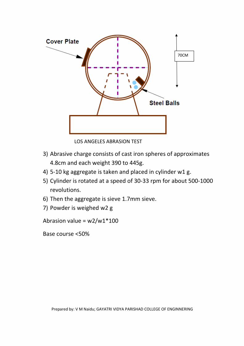
LOS ANGELES ABRASION TEST:
1) Steel balls are used as abrasive charge.
2) Machine consists of a hollow cylinder having 70cm diameter,
length 50cm.
Prepared by: V M Naidu; GAYATRI VIDYA PARISHAD COLLEGE OF ENGINNERING
LOS ANGELES ABRASION TEST
3) Abrasive charge consists of cast iron spheres of approximates
4.8cm and each weight 390 to 445g.
4) 5-10 kg aggregate is taken and placed in cylinder w1 g.
5) Cylinder is rotated at a speed of 30-33 rpm for about 500-1000
revolutions.
6) Then the aggregate is sieve 1.7mm sieve.
7) Powder is weighed w2 g
Abrasion value = w2/w1*100
Base course <50%
70CM

Prepared by: V M Naidu; GAYATRI VIDYA PARISHAD COLLEGE OF ENGINNERING
DEVAL ABRASION TEST:
30-33 rpm, 10000 revolutions
Prepared by: V M Naidu; GAYATRI VIDYA PARISHAD COLLEGE OF ENGINNERING
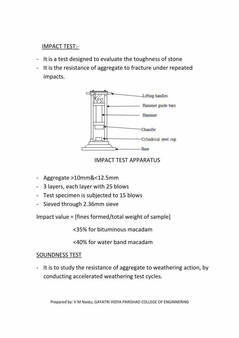
IMPACT TEST:-
- It is a test designed to evaluate the toughness of stone
- It is the resistance of aggregate to fracture under repeated
impacts.
IMPACT TEST APPARATUS
- Aggregate >10mm&<12.5mm
- 3 layers, each layer with 25 blows
- Test specimen is subjected to 15 blows
- Sieved through 2.36mm sieve
Impact value = [fines formed/total weight of sample]
<35% for bituminous macadam
<40% for water band macadam
SOUNDNESS TEST
- It is to study the resistance of aggregate to weathering action, by
conducting accelerated weathering test cycles.
Prepared by: V M Naidu; GAYATRI VIDYA PARISHAD COLLEGE OF ENGINNERING
- It is the resistance to disintegration of aggregate by using
saturated solution of sodium sulphate (or) magnesium sulphate
- Take clean, dry aggregate specimen of specified size range and is
weighed and counted.
- It is immersed in sodium sulphate (or) magnesium sulphate for
16-18 hours.
- It is dried in oven at 105-110˚c.
- Again immerse in chemical solution & dry it.
- Repeat this for 10 cycles.
- Check the weights of aggregates
Avg loss in weight ≤ 12% (for sodium sulphate)
≤ 18% (for magnesium sulphate)
SHAPE TESTS:
- This is conducted to determine percentage of flaky and elongated
particles.
- The elevation of shape of the partical made in terms of flakiness
index, elongation index and angularity number.
SPECIFIC GRAVITY AND WATER ABSORPTION TEST
- Specific gravity is considered to measure the quality and strength
of material.
- Stones having low specific gravity are weaker.
- Stones having higher water absorption are weak.
STEP: 1 - Take about 2 kg of dry aggregate and is placed in wire
bucket and is immersed in 24 hours.
STEP: 2- the sample is weighed in water and buoyant weight is
found.

Prepared by: V M Naidu; GAYATRI VIDYA PARISHAD COLLEGE OF ENGINNERING
Aggregate is dried in oven for 24 hours at a temperature of 100-
110˚c and then dry weight is determined.
� Specific gravity = [dry weight of aggregate/weight of equal volume
of water]
=2.6-2.9
� Water absorption = [water absorbed/oven dried weight of
aggregate]
≤0.6%
BITUMEN MATERIALS:
� This is a binding material used in pavement construction.
� It is produced by distillation of petroleum crude where as tar is
obtained by destructive distillation of coal or wood.
� Both bitumen, tar have similar appearance, bulk in color, but they
have different characteristics.
� When the bitumen contains some inert material (or) mineral, it is
called asphalt.
� The grades of bitumen used for pavement construction work for
roads and airfields are called paving grades.
� The grades used for water proofing of structures and industrial
floors etc., are called industrial grades.
• Paving bitumen from assam petroleum, denoted as A-type and
designed as grades A35, A90 etc.
• Pavement bitumen from other sources denoted as S-type and
designated as grades S35, S90 etc.
TESTS ON BITUMEN:
The various tests on bituminous material are

Prepared by: V M Naidu; GAYATRI VIDYA PARISHAD COLLEGE OF ENGINNERING
a) Penetration tests
b) Ductility tests
c) Viscosity tests
d) Float tests
e) Specific gravity test
f) Softening point test
g) Flash and fire point test
h) Solubility test
i) Spot test
j) Loss on heating test
k) Water content test
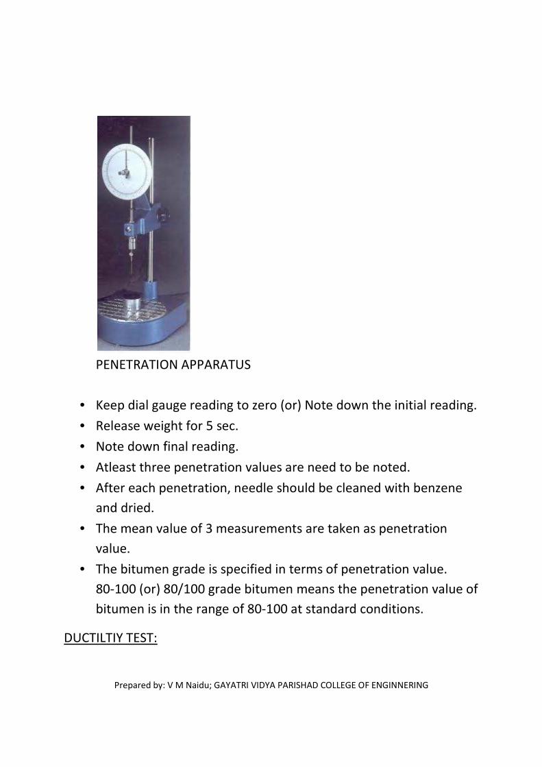
PENETRATION TEST:
• This test determines the hardness or softness of bitumen by
measuring the depth in terms of millimeter vertically in 5 sec.
Sample is prepared and kept water at controlled temperature
25˚c
Prepared by: V M Naidu; GAYATRI VIDYA PARISHAD COLLEGE OF ENGINNERING
PENETRATION APPARATUS
• Keep dial gauge reading to zero (or) Note down the initial reading.
• Release weight for 5 sec.
• Note down final reading.
• Atleast three penetration values are need to be noted.
• After each penetration, needle should be cleaned with benzene
and dried.
• The mean value of 3 measurements are taken as penetration
value.
• The bitumen grade is specified in terms of penetration value.
80-100 (or) 80/100 grade bitumen means the penetration value of
bitumen is in the range of 80-100 at standard conditions.
DUCTILTIY TEST:
Prepared by: V M Naidu; GAYATRI VIDYA PARISHAD COLLEGE OF ENGINNERING
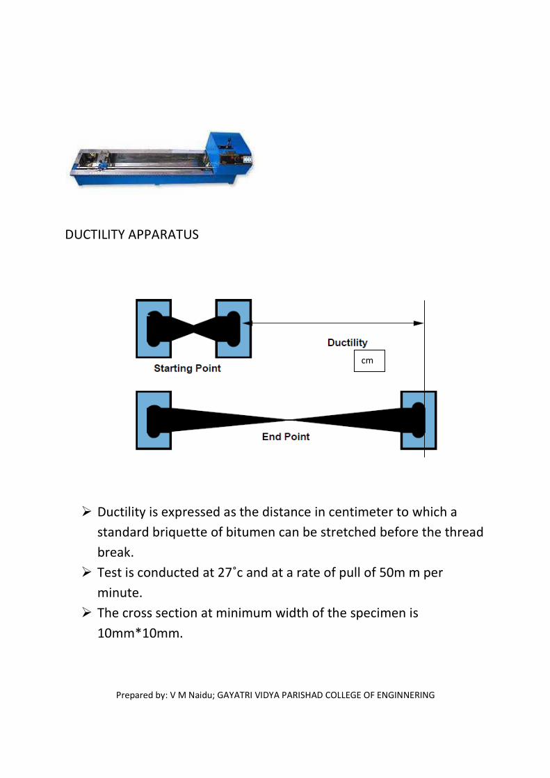
DUCTILITY APPARATUS
� Ductility is expressed as the distance in centimeter to which a
standard briquette of bitumen can be stretched before the thread
break.
� Test is conducted at 27˚c and at a rate of pull of 50m m per
minute.
� The cross section at minimum width of the specimen is
10mm*10mm.
cm
Prepared by: V M Naidu; GAYATRI VIDYA PARISHAD COLLEGE OF ENGINNERING
� The ductility machine functions as a constant temperature water
bath with a pulling device at a pre-calibrated rate.
� Ductility values of bitumen vary from 5 to 100 for different
grades.
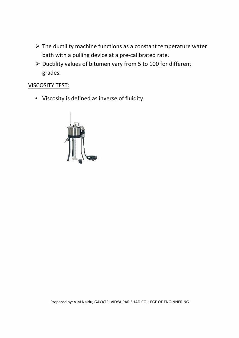
VISCOSITY TEST:
• Viscosity is defined as inverse of fluidity.

Prepared by: V M Naidu; GAYATRI VIDYA PARISHAD COLLEGE OF ENGINNERING
• It is fluid property of bituminous material
• It is measure of resistance of flow.
• Orifice type viscometer may be used to indirectly find the viscosity
of liquid binder.
• Viscosity of tar is determined as the time taken in seconds for
50ml of the sample to flow through 10mm orifice.
FLOAT TEST:
Bituminous material
Water at 50˚c
Water at 50˚c
Float test set up
Prepared by: V M Naidu; GAYATRI VIDYA PARISHAD COLLEGE OF ENGINNERING
• The apparatus consists of a float material made of aluminium and
a brass collar filled with specimen materials to be tested.
• The test specimen is filled in the collar, cooled to a temperature of
5˚c.
• The float assembly is floated in a water bath at 50˚c and the time
required in seconds for water to force its way through the
bitumen plug is noted as the float test value.
• Higher the float test value, the stiffer the material.
SPECIFIC GRAVITY TEST:
• The specific value of bitumen is useful in bituminous mix design.
• Increase amounts of aromatic type compounds (or) mineral
impurities cause an increase in specific gravity.
• Specific gravity of bituminous materials is defined as the ratio of
the mass of given value of substance to the same of an equal
volume of water.
• Specific gravity is determined by pycnometer
• Generally, the specific gravity of pure bitumen is in range of 0.97
to 1.02.
SOFTENING POINT TEST:
� The softening is the temperature at which the substance attains a
particular degree of softening under specified condition of test.
� This test is usually conducted by Ring and Ball apparatus.

Prepared by: V M Naidu; GAYATRI VIDYA PARISHAD COLLEGE OF ENGINNERING
SOFTENING POINT TEST
� Higher softening point indicates lower susceptibility.
� Softening point of various bitumen grades vary between 35˚c to
70˚c.
FLASH AND FIRE POINT TEST:
� Flash point of the material is the lowest temperature at which the
vapour of substance momentarily takes fire in the form of flash.
� Fire point is the lowest temperature at which the material gets
ignited and burns under specified conditions of test.

Prepared by: V M Naidu; GAYATRI VIDYA PARISHAD COLLEGE OF ENGINNERING
FLASH AND FIRE POINT APPARATUS
REQUIREMEMNTS OF BITUMEN MIXES:
The mix design should aim at an economical blend, with
proper gradation of aggregates and adequate proportion of
bitumen so as to fulfill the desired properties of mix.
The desirable properties of a good bituminous mix are
stability, durability, flexibility, skid resistance and
workability.
Stability is defined as resistance of paving mix to
deformation under load. It is the stress which causes specific
strain.
Stability is function of friction and cohesion
• Friction: It is function of both inter particle friction and
friction imparted by bituminous material.
• Cohesion: It is mainly offered by factors that influence
the mass viscosity of bitumen binder.
Durability is defined as the resistance of mix against
weathering and abrasive action.
Flexibility is a property of the mix that measures the level
bending strength.
Skid resistance is defined as the resistance of the finished
pavement against skidding and is a function of surface
texture and bitumen content.
Workability is the ease with which the mix can be laid and
compacted. It is the function of grade, shape and texture of
aggregate and bitumen content.
MIX DESIGN REQUIRES FOLLOWING PROPERTIES:
Prepared by: V M Naidu; GAYATRI VIDYA PARISHAD COLLEGE OF ENGINNERING
� Sufficient stability to satisfy service requirements of the
pavement and traffic conditions, without undue
displacements.
� Sufficient durability by coating aggregates and bonding
them together and also by water-proofing the mix.
� Sufficient voids in the compacted mix.
� Sufficient flexibility even in the coldest season to prevent
cracking due to repeated application of traffic load.
� Sufficient workability while placing and compacting the
mix.
� The mix should be the most economical one that would
produce a stable, durable, and skid resistant pavement.
Other tests on bitumen are:
(a) Solubility test(weight of insoluble material/weight of original
sample)
(b)Spot test (to test over-heated bitumen)
(c) Loss on heating (loss in weight due to heating)
(d) Water content test.
MARSHALL METHOD OF BITUMINOUS MIX DESIGN:
Marshall, formerly bituminous engineer with Mississipi
State Highway Department formulated this method.
In this method, the resistance to plastic deformation of
cylindrical specimen of bituminous mixture is measured

Prepared by: V M Naidu; GAYATRI VIDYA PARISHAD COLLEGE OF ENGINNERING
when the same loaded at the periphery at a rate of
5cm/min.
There are two major features of Marshall method of
designing mixes, namely:
(1) Density void analysis, and
(2) Stability flow test.
Stability of the mix is defined as a maximum load carried
by a compacted specimen at a standard test temperature
60˚c.
Flow is measured as the deformation in units of 0.25mm
between no load and maximum load carried by the
specimen during stability test.
Approximately 1200 g of mixed aggregates and the filler
are taken and heated to a temperature of 175˚c to 190˚c.
The bitumen is heated to a temperature of 121˚c to
145˚c and required quantity of the first trial percentage
of bitumen (say 3.5% or 4% by weight of material
aggregate) is added to the heated aggregates and
thoroughly mixed at the desired temperature of 154˚c to
160˚c.
Apparatus consists of 10.16cm diameter and 6.35 cm
height, with a base plate and a collar.
A compaction pedestal and hammer are used to compact
a specimen by 4.54kg weight with 45.7cm height of fall.
The mix is placed in preheated mould and compacted by
rammer with 50 blows on either side.

Prepared by: V M Naidu; GAYATRI VIDYA PARISHAD COLLEGE OF ENGINNERING
The compacted specimens are cooled to room
temperature and then extracted from the mould with the
help of specimen extractor.
Three or four specimens may be prepared using each
trial bitumen content.
The diameter and mean height of specimen are
measured and they are weighed in air and water.
The specimen are kept immersed in water in
thermostatically controlled water bath at 60˚c for 30-40
min.
Specimens are taken one-by-one, placed in Marshall test
head and tested to determine Marshall’s Stability value
and flow value.
Load is applied on its periphery perpendicular to its axis
in a loading machine of 5tonnes capacity at a rate of
5cm/min.
Dial gauge fixed to the guide rods acts as a flow meter to
measure the deformation of the specimen during
loading.

Prepared by: V M Naidu; GAYATRI VIDYA PARISHAD COLLEGE OF ENGINNERING
Correction factor should be applied to Marshall’s Stability
value, the average height of specimen is not exactly
63.5mm.
Same above procedure is applied with other bitumen
content with increment of 0.5%, upto about 7.5%-8%
bitumen by weight of total mix.
Percentage of air voids, Vv= (Gt-Gm)/Gm *100
Here Gm= bulk density (or) mass density of the specimen.
Gt= theoritical specific gravity of mixture.
Gt = 1000/ ((w1/g1) + (w2/g2) + (w3/g3) + (w4/g4))
Where
W1= percentage by weight of coarse aggregate in to total mix.
W2= percentage by weight of fine aggregate in total mix.
Prepared by: V M Naidu; GAYATRI VIDYA PARISHAD COLLEGE OF ENGINNERING
W3= percentage by weight of filler aggregate in total mix.
W4= percentage by weight of bitumen in total mix.
G1=apparent specific gravity of coarse aggregate.
G2=apparent specific gravity of fine aggregate.
G3=apparent specific gravity of filler aggregate.
G4=apparent specific gravity of bitumen aggregate.
Percent voids in mineral aggregate (VMA)
VMA=VV+VB
Where volume bitumen VB= GM* (W4/G4)*100
VFB= (VB/VMA)*100
Prepared by: V M Naidu; GAYATRI VIDYA PARISHAD COLLEGE OF ENGINNERING
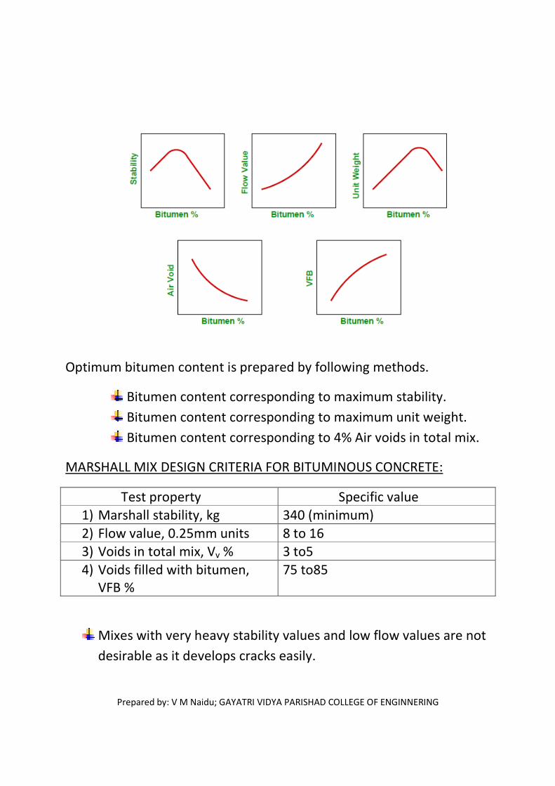
Optimum bitumen content is prepared by following methods.
Bitumen content corresponding to maximum stability.
Bitumen content corresponding to maximum unit weight.
Bitumen content corresponding to 4% Air voids in total mix.
MARSHALL MIX DESIGN CRITERIA FOR BITUMINOUS CONCRETE:
Test property Specific value
1) Marshall stability, kg 340 (minimum)
2) Flow value, 0.25mm units 8 to 16
3) Voids in total mix, Vv % 3 to5
4) Voids filled with bitumen,
VFB %
75 to85
Mixes with very heavy stability values and low flow values are not
desirable as it develops cracks easily.

Prepared by: V M Naidu; GAYATRI VIDYA PARISHAD COLLEGE OF ENGINNERING
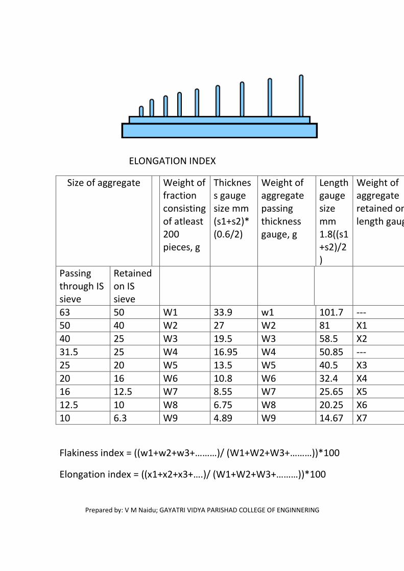
SHAPE TEST OF AGGREGATE:
This test is performed to calculate flakiness index, elongation
index.
Flakiness index aggregates is the percentages by weight of
particles whose least dimension is less than three-fifth (0.6) of
their dimension.
Elongation index of an aggregate is the percentage by weight of
particles whose greatest dimension (length) is greater than one
and four-fifth (1.8 times) their mean dimension.
FLAKINESS INDEX
Prepared by: V M Naidu; GAYATRI VIDYA PARISHAD COLLEGE OF ENGINNERING
ELONGATION INDEX
Size of aggregate Weight of
fraction
consisting
of atleast
200
pieces, g
Thicknes
s gauge
size mm
(s1+s2)*
(0.6/2)
Weight of
aggregate
passing
thickness
gauge, g
Length
gauge
size
mm
1.8((s1
+s2)/2
)
Weight of
aggregate
retained on
length gauge, g
Passing
through IS
sieve
Retained
on IS
sieve
63 50 W1 33.9 w1 101.7 ---
50 40 W2 27 W2 81 X1
40 25 W3 19.5 W3 58.5 X2
31.5 25 W4 16.95 W4 50.85 ---
25 20 W5 13.5 W5 40.5 X3
20 16 W6 10.8 W6 32.4 X4
16 12.5 W7 8.55 W7 25.65 X5
12.5 10 W8 6.75 W8 20.25 X6
10 6.3 W9 4.89 W9 14.67 X7
Flakiness index = ((w1+w2+w3+………)/ (W1+W2+W3+………))*100
Elongation index = ((x1+x2+x3+….)/ (W1+W2+W3+………))*100

Prepared by: V M Naidu; GAYATRI VIDYA PARISHAD COLLEGE OF ENGINNERING
In pavement construction, flaky and elongated particles are to be
avoided.
UNIT: 3
HIGHWAY GEOMETRIC DESIGN
Importance of geometric design:
Geometric design of highway deals with dimensions and layout of
visible features of highway such as sight distances and
intersections.
Geometrics are designed to provide optimum efficiency in traffic
operations with maximum safety at reasonable cost.
Geometric design of highways deals with following elements:
1) Cross section elements.
2) Sight distance considerations.
3) Horizontal alignment.
4) Vertical alignment.
5) Intersection elements.
DESIGN CONTROLS AND CRITERIA:
Geometric design of highway depends on several factors.
The important of these factors are:
a) Design speed.
b) Topography.
c) Traffic factors.
d) Design hourly volume and capacity.

Prepared by: V M Naidu; GAYATRI VIDYA PARISHAD COLLEGE OF ENGINNERING
e) Environmental and other factors.
a) Design speed:
It is the important factor which controls the geometric
design.
Design speed is decided based on the category of the road.
i.e NH, SH, MDR, ODR and VR.
Urban roads have different set of design speeds.
Design of almost all the elements of the highway dependent
on design speed.
Width of the road, sight distance requirements, the
horizontal alignment elements such as radius of curve,
super elevation, transition curve length and vertical
alignment elements such as valley, summit curve lengths-all
these depend mainly on design speed.
b) Topography:
Topography plays vital role in geometric design.
Based on topography, the longitudinal slopes are
provided.
In hilly terrain, it is necessary to allow for steeper
gradients and sharper horizontal curves.
c) Traffic factors:
The factors associated with traffic are vehicle
characteristics and human characteristics.
The different vehicle classes such as bus, car, truck, motor
cycles have different speeds and acceleration
characteristics apart from having different dimensions and
weights.
Prepared by: V M Naidu; GAYATRI VIDYA PARISHAD COLLEGE OF ENGINNERING
Important human factors which affect traffic behavior
include physical, mental and psychological characteristics
of driver and pedestrian.
d) Design hourly volume and capacity:
Traffic keeps on changing in peak and in off-peak
periods.
It experiences highest in peak and low in off-peak
periods.
It is uneconomical to design roadway for peak period.
So, a reasonable value of traffic volume is decided for
design and this is called design hourly volume.
The ratio of volume to capacity reflects the level of
service of road.
e) Environmental and other factors:
The environmental factors such as aesthetics,
landscaping, air pollution, noise pollution should be
considered while designing road geometrics.
HIGHWAY CROSS SECTION ELEMENTS:
PAVEMENT SURFACE CHARACTERISTICS:
• The important surface characteristics of the pavement are
friction, unevenness, light reflecting characteristics and
drainage of surface water.
Friction
When a vehicle negotiates a horizontal curve, the
lateral friction developed counteracts the centrifugal
force and thus governs the safe operating speed.

Prepared by: V M Naidu; GAYATRI VIDYA PARISHAD COLLEGE OF ENGINNERING
• Skid: when the path travelled by the vehicle is more than
circumferential movement, then it is called skid.
• Slip: when the wheel revolves more than the
corresponding longitudinal movement along the road.
Factors affecting friction (or) skid resistance:
a) Type of pavement surface (C.C, WBM, Earth surface etc)
b) Macro-texture.
c) Condition of pavement(wet, dry)
d) Type and condition of tyre.
e) Speed of vehicle.
f) Brake efficiency.
g) Load and tyre pressure.
h) Temperature of tyre and pavement.
i) Type of skid.
PAVEMENT UNEVENNESS:
Higher operating speeds are possible on even
pavement surface than on uneven and poor
surfaces.
Bump integrater is commonly used to measure
pavement surface condition in terms of unevenness
index.
Unevenness index is the cumulative measure of
vertical undulations of the pavement surface
recorded per unit horizontal length of road.
Good - 150cm/km.
Satisfactory – 250cm/km
Uncomfortable – 350cm/km

Prepared by: V M Naidu; GAYATRI VIDYA PARISHAD COLLEGE OF ENGINNERING
FACTORS CAUSING UNEVENNESS:
a) Inadequate compaction of sub aggregate.
b) Un-scientific construction practices.
c) Use of inferior material.
d) Use of improper machinery.
e) Improper surface drainage.
f) Poor maintenance practices.
g) Localized failures.
LIGHT REFLECTING CHARATERISTICS:
Night visibility depend on light reflecting characteristics
of pavement surface.
Glare caused on wet pavement surface is more than dry
surface.
CROSS SLOPE (or) CAMBER:
It is the slope provided to the road surface in transverse
direction to drain off rain water from road surface.
Cross slope is important due to following reasons:
• To prevent the entry of surface water into the sub-
grade soil.
• To prevent entry of water in to bituminous pavement
layers.
• To remove the rain water from pavement surface.
It is denoted in 1 in ‘n’ and x%.
Flat camber of 1.7 to 2.0% is sufficient.

Prepared by: V M Naidu; GAYATRI VIDYA PARISHAD COLLEGE OF ENGINNERING
Too steep cross slope in undesirable because of following
reasons:-
1) Transverse tilt of vehicles causing uncomfortable side thrust.
2) Discomfort.
3) Problems of toppling.
4) Formation of cross ruts.

Prepared by: V M Naidu; GAYATRI VIDYA PARISHAD COLLEGE OF ENGINNERING
SHAPE OF CROSS SLOPE:
Different types of cambers
Prepared by: V M Naidu; GAYATRI VIDYA PARISHAD COLLEGE OF ENGINNERING
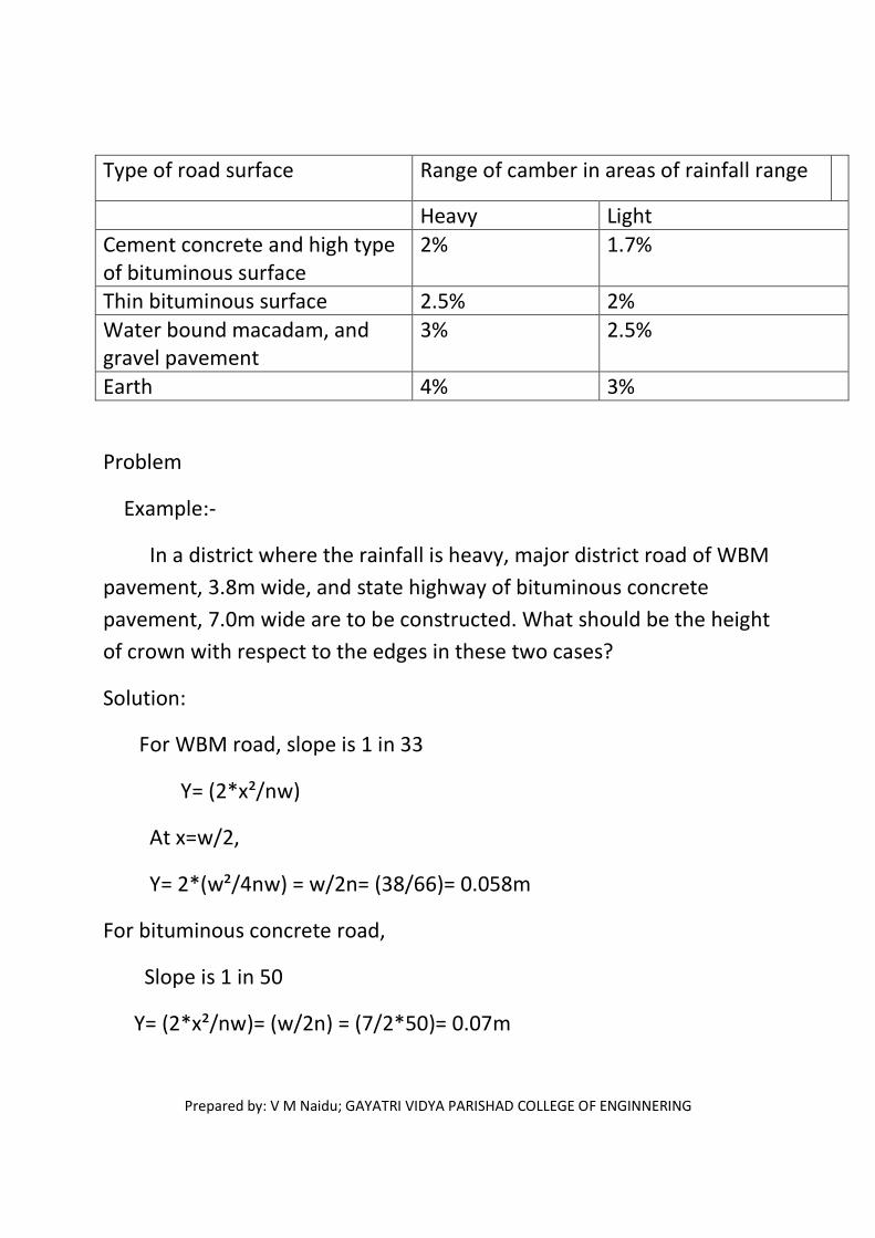
Type of road surface Range of camber in areas of rainfall range
Heavy Light
Cement concrete and high type
of bituminous surface
2% 1.7%
Thin bituminous surface 2.5% 2%
Water bound macadam, and
gravel pavement
3% 2.5%
Earth 4% 3%
Problem
Example:-
In a district where the rainfall is heavy, major district road of WBM
pavement, 3.8m wide, and state highway of bituminous concrete
pavement, 7.0m wide are to be constructed. What should be the height
of crown with respect to the edges in these two cases?
Solution:
For WBM road, slope is 1 in 33
Y= (2*x²/nw)
At x=w/2,
Y= 2*(w²/4nw) = w/2n= (38/66)= 0.058m
For bituminous concrete road,
Slope is 1 in 50
Y= (2*x²/nw)= (w/2n) = (7/2*50)= 0.07m

Prepared by: V M Naidu; GAYATRI VIDYA PARISHAD COLLEGE OF ENGINNERING
WIDTH OF PAVEMENT OR CARRIAGE WAY :-
• It depends on width of traffic lane and no. of lanes.
• The carriageway intended for one line of traffic movement is
called as traffic lane.
Class of road Width of carriage way
TRAFFIC SEPERATOR (OR) MEDIANS:-
• The main function of traffic separator is to prevent head-on
collision between vehicles moving in opposite directions on
adjacent lanes.
It may also helps to
1) Channelise traffic in to streams at intersection

Prepared by: V M Naidu; GAYATRI VIDYA PARISHAD COLLEGE OF ENGINNERING
2) Shadow the crossing and turning traffic
3) Segregate slow traffic and to protect pedestrians.
IRC recommends a minimum desirable width of 5.0 m for medians of
rural highways, which may be reduced to 3.0m where land is restricted.
On long bridges the width of the median may be reduced up to 1.2 to
1.5m
KERB:
� It indicates the boundary between the pavement and shoulder
(or) island (or) footpath (or) kerb parking.
Different types of kerbs
1) low (or) mountable type kerbs
Prepared by: V M Naidu; GAYATRI VIDYA PARISHAD COLLEGE OF ENGINNERING
2) Semi-barrier type kerbs
3) Barrier type kerb
4) Submerged kerbs
Road margins:
The various elements included in the road margins aree shoulders,
parking lane, frontage road, drive way, cycle track, footpath, guard rails.
Width of roadway (or) formation:
� it is the sum of widths of pavements (or) carriage way including
separators and the shoulders.
� It is the top width of highway embankment (or) bottom width of
highway cutting.
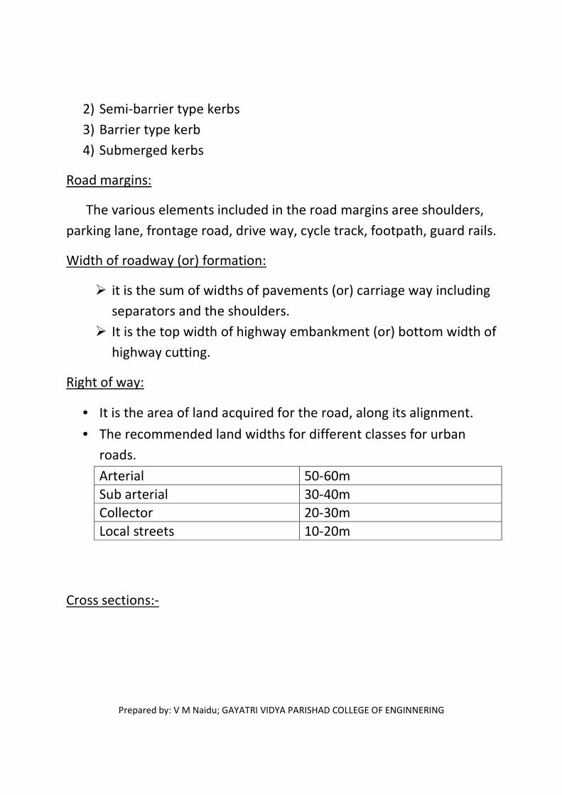
Right of way:
• It is the area of land acquired for the road, along its alignment.
• The recommended land widths for different classes for urban
roads.
Arterial 50-60m
Sub arterial 30-40m
Collector 20-30m
Local streets 10-20m
Cross sections:-
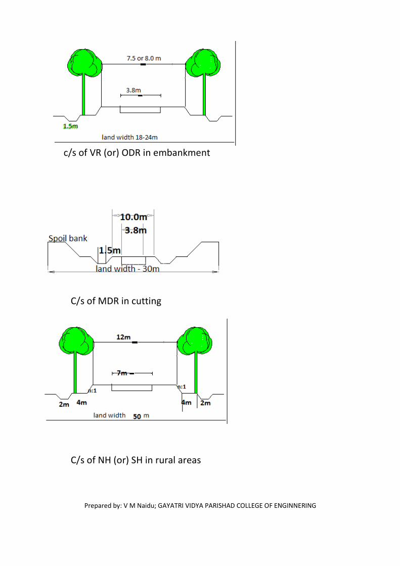
Prepared by: V M Naidu; GAYATRI VIDYA PARISHAD COLLEGE OF ENGINNERING
c/s of VR (or) ODR in embankment
C/s of MDR in cutting
C/s of NH (or) SH in rural areas

Prepared by: V M Naidu; GAYATRI VIDYA PARISHAD COLLEGE OF ENGINNERING
C/s of two-lane city road
C/s of divided highway in Urban
Sight distance:
• It is the actual distance along the road surface, which a driver
from a specified height above the carriage way has visibility of
stationary (or) moving objects.
• It is the length of road visible ahead to driver at any instance.
Prepared by: V M Naidu; GAYATRI VIDYA PARISHAD COLLEGE OF ENGINNERING
In design, the following sight distances are considered
1) Stopping (or) absolute minimum sight distances are
calculated.
2) Safe overtaking (or) passing sight distance.
3) Safe sight distance for entering in to uncontrolled
intersections.
Intermediate sight distance:
• It is defined as twice the stopping sight distance
• When the overtaking sight distance cannot be provided, the
intermediate sight distance is provided to give limited
overtaking opportunities to fast vehicle.
Stopping sight distance:
• It is the length taken to stop a vehicle travelling at design speed,
safely without collision with any other obstruction.
Sight distance depends on
• Feature of the road ahead.
• Height of driver’s eye above the road surface.
• Height of object above road surface.
IRC has suggested the height of the eye level of driver as 1.2m and
height of the object as 0.15m above road surface.
Stopping sight distance depends on factors:
• Total reaction time of the driver.
• Speed of the vehicle.
• Efficiency of breaks.

Prepared by: V M Naidu; GAYATRI VIDYA PARISHAD COLLEGE OF ENGINNERING
• Friction resistance between road and tyre.
• Gradient of the road.
PIEV THEORY:
Perception time:
It is the time required for sensations received by eye (or)
ear to be transmitted to the brain.
Intellection time:
Time required to understand the situation.
Emotion time:
Time elapsed during emotional sensations and
disturbance such as fear, anger.
Volition time:
It is the time taken for final action.

Prepared by: V M Naidu; GAYATRI VIDYA PARISHAD COLLEGE OF ENGINNERING
Stopping distance:
It is the sum of
1) The distance travelled by the vehicle during the total reaction
time (lag distance).
2) The distance travelled by the vehicle after the application of
brakes, to a dead stop position (braking distance).
Prepared by: V M Naidu; GAYATRI VIDYA PARISHAD COLLEGE OF ENGINNERING
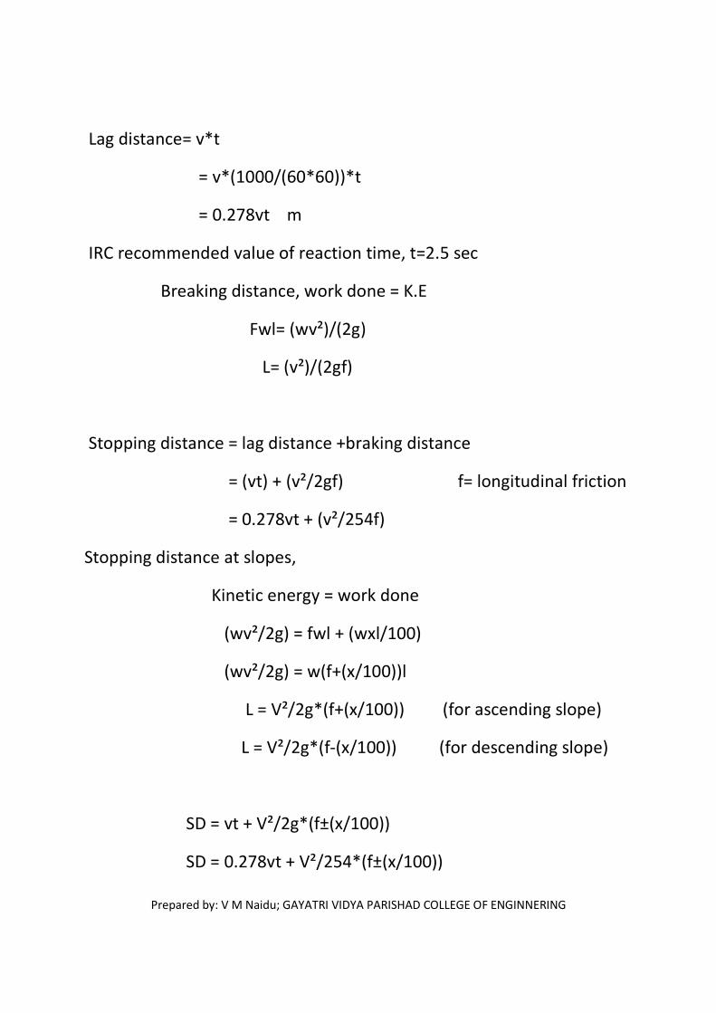
Lag distance= v*t
= v*(1000/(60*60))*t
= 0.278vt m
IRC recommended value of reaction time, t=2.5 sec
Breaking distance, work done = K.E
Fwl= (wv²)/(2g)
L= (v²)/(2gf)
Stopping distance = lag distance +braking distance
= (vt) + (v²/2gf) f= longitudinal friction
= 0.278vt + (v²/254f)
Stopping distance at slopes,
Kinetic energy = work done
(wv²/2g) = fwl + (wxl/100)
(wv²/2g) = w(f+(x/100))l
L = V²/2g*(f+(x/100)) (for ascending slope)
L = V²/2g*(f-(x/100)) (for descending slope)
SD = vt + V²/2g*(f±(x/100))
SD = 0.278vt + V²/254*(f±(x/100))
Prepared by: V M Naidu; GAYATRI VIDYA PARISHAD COLLEGE OF ENGINNERING
Eg:-
Calculate the safe stopping for design speed of 50 kmph for (a)two-
way traffic on a two lane road (b) two-way traffic on a single lane road.?
Sol: Assume coefficient of friction as 0.37 and reaction time of driver
as 2.5 sec
SD = 0.278vt + (v²/254f)
= 0.278*50*2.5 + (50²/254*0.37)
=61.4m
Stopping sight distance when there are two lanes= stopping
distance= 61.4m
Stopping sight distance with single lane= 2*64.1 =122.8m
Eg:-
Calculate the minimum sight distance required to avoid a head-on
collision of two cars approaching from the opposite direction at 90 and
60 kmph. Assume a reaction time of 2.5 sec, coefficient of friction of 0.7
and brake efficiency 50%?
Sol: f= 0.5*0.7 = 0.35
Stopping sight distance for first car, SD1= 0.278vt + (V²/254f)
= 0.278*90*2.5 +(90²/(254*0.35))
=153.6m
For second car, SD2= 0.278vt + (V²/254f)

Prepared by: V M Naidu; GAYATRI VIDYA PARISHAD COLLEGE OF ENGINNERING
= 0.278*60*2.5 + (60²/(254*0.35))
=82.2m
Sight distance to avoid head-on collision of two
approaching cars = SD1+SD2
= 153.2+82.2
=235.4m
Eg:-
Calculate the stopping sight distance on a highway at a descending
gradient of 2% for a design speed of 80kmph. Assume other data as per
IRC recommendations
Sol :- t=2.5s, f= 0.35
V=80kmph, x= -2%
SSD = 0.278vt + (V²/254*(f-0.02))
=0.278*80*2.5 + (80²/(254*(0.35-0.02)))
=55.6 +76.4
=132m
Eg:-
Calculate the values of a) Head light sight distance b) intermediate
sight distance for a highway with speed 65kmph. Assume suitable data

Prepared by: V M Naidu; GAYATRI VIDYA PARISHAD COLLEGE OF ENGINNERING
Sol: v=65kmph, f= 0.35, t= 2.5 sec
a) Head light sight distance, SSD = (0.278*vt) + (V²/254f)
= (0.278*65*2.5) + (65²/(254*0.35))
= 91.4m
b) Intermediate sight distance = 2* SSD
= 2*91.4
= 182.8m
Overtaking sight distance:-
Different vehicles travels with different speeds.
If all the vehicles travel with design speed, then there is
no need of overtaking. But it is not possible.
The minimum distance open to the vision of the driver of
a vehicle intending to overtake slow vehicle ahead with
safety against the traffic of opposite direction is known as
“OSD”.
OSD depends on
a) Speeds of overtaking vehicle, overtaken vehicle and the vehicle
coming from the opposite direction.
b) Distance between overtaking and overtaken vehicle
c) Skill and reaction time of driver.
d) Rate of acceleration of overtaking vehicle
e) Gradation of the road.
Prepared by: V M Naidu; GAYATRI VIDYA PARISHAD COLLEGE OF ENGINNERING
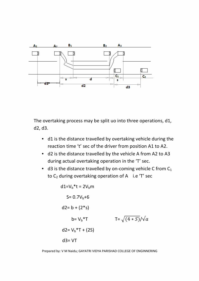
The overtaking process may be split uo into three operations, d1,
d2, d3.
• d1 is the distance travelled by overtaking vehicle during the
reaction time ‘t’ sec of the driver from position A1 to A2.
• d2 is the distance travelled by the vehicle A from A2 to A3
during actual overtaking operation in the ‘T’ sec.
• d3 is the distance travelled by on-coming vehicle C from C1
to C2 during overtaking operation of A i.e ‘T’ sec
d1=Vb*t = 2Vbm
S= 0.7Vb+6
d2= b + (2*s)
b= Vb*T T= �(4 ∗ �)/√�
d2= Vb*T + (2S)
d3= VT

Prepared by: V M Naidu; GAYATRI VIDYA PARISHAD COLLEGE OF ENGINNERING
OSD = d1+d2+d3
= Vbt + VbT + 2S + VT
OSD = 0.278Vbt + 0.278VbT + 2S + 0.278VT
Effect of grade in overtaking sight distance:-
Both descending as well as ascending, increase the sight distance
required for safe overtaking.
Overtaking zones:
Minimum length of overtaking zone = 3*OSD
Prepared by: V M Naidu; GAYATRI VIDYA PARISHAD COLLEGE OF ENGINNERING
= 3*(d1+d2+d3) (two-way)
= 3*(d1+d2) (one-way)
Desirable length of overtaking zone = 5*OSD
= 5*(d1+d2+d3) (two-way)
= 5*(d1+d2) (one-way)
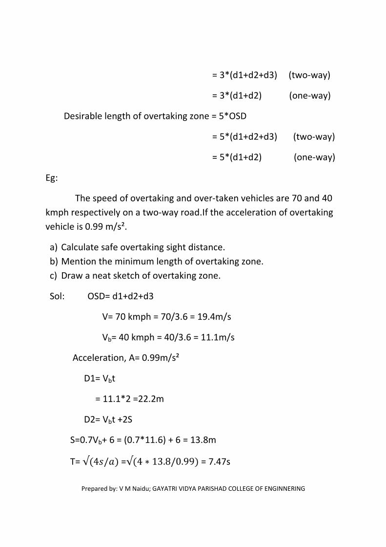
Eg:
The speed of overtaking and over-taken vehicles are 70 and 40
kmph respectively on a two-way road.If the acceleration of overtaking
vehicle is 0.99 m/s².
a) Calculate safe overtaking sight distance.
b) Mention the minimum length of overtaking zone.
c) Draw a neat sketch of overtaking zone.
Sol: OSD= d1+d2+d3
V= 70 kmph = 70/3.6 = 19.4m/s
Vb= 40 kmph = 40/3.6 = 11.1m/s
Acceleration, A= 0.99m/s²
D1= Vbt
= 11.1*2 =22.2m
D2= Vbt +2S
S=0.7Vb+ 6 = (0.7*11.6) + 6 = 13.8m
T= √(4/�) =√(4 ∗ 13.8/0.99) = 7.47s

Prepared by: V M Naidu; GAYATRI VIDYA PARISHAD COLLEGE OF ENGINNERING
D2= (11.1*7.47) +(2*13.8)
= 110.5m
D3=VT= (19.4*7.47) = 144.9m
OSD = d1+d2+d3
= 22.2+110.5+144.9
= 277.6m = 278m
Minimum length of overtaking zone =3*OSD
= 3*278
=834m
Desirable length of overtaking zone = 5*OSD
= 5*278 = 1390m
SP1=overtaking zone ahead.
SP2=end of overtaking zone.
Eg:
Calculate the safe overtaking sight distance for a design speed of 96
kmph. Assume suitable data.

Prepared by: V M Naidu; GAYATRI VIDYA PARISHAD COLLEGE OF ENGINNERING
SOL:
OSD = d1+d2 (for one-way traffic)
= d1+d2+d3 (for two-way traffic)
V=96kmph
Assume Vb= V-16=80kmph
A = 2.5kmph/sec, t= 2sec
D1= 0.278VbT= 0.278*80*2 = 44.8m
D2= 0.278VbT+ 2s
S=0.2Vb+6
= (0.2*80)+6= 22m
T=√(14.4/�) = √(14.4 ∗ 22/2.5) =11.3sec
D2= (0.278*80*11.3) + (2*22)
= 297m
D3= 0.278VT = 0.278*96*11.3 = 303.7m
OSD0ne-way= d1+ d2 = 44.8+297 = 341.8= 342m
OSDTwo-way=d1+d2+d3= 44.8+297+303.7=645.5m

Prepared by: V M Naidu; GAYATRI VIDYA PARISHAD COLLEGE OF ENGINNERING
Sight distance at intersection:
Prepared by: V M Naidu; GAYATRI VIDYA PARISHAD COLLEGE OF ENGINNERING
UNIT-4
HIGHWAY GEOMETRIC DESIGN-2
Design of horizontal alignment:-
Factors to be considered are
a) Design speed.
b) Radius of circular curves.
c) Type of road and length of transition curves.
d) Super-elevation
e) Extra widening of pavement on curves
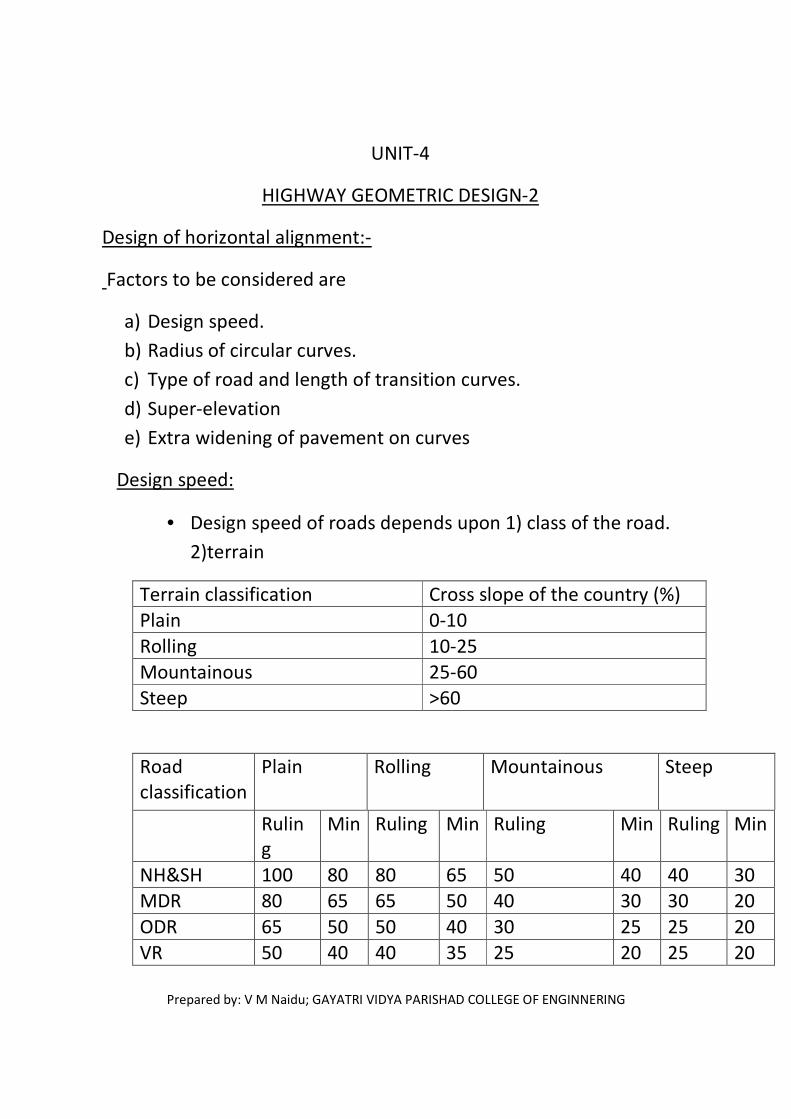
Design speed:
• Design speed of roads depends upon 1) class of the road.
2)terrain
Terrain classification Cross slope of the country (%)
Plain 0-10
Rolling 10-25
Mountainous 25-60
Steep >60
Road
classification
Plain Rolling Mountainous Steep
Rulin
g
Min Ruling Min Ruling Min Ruling Min
NH&SH 100 80 80 65 50 40 40 30
MDR 80 65 65 50 40 30 30 20
ODR 65 50 50 40 30 25 25 20
VR 50 40 40 35 25 20 25 20

Prepared by: V M Naidu; GAYATRI VIDYA PARISHAD COLLEGE OF ENGINNERING
Recommended design speeds for different classes of urban roads.
a) For arterial roads 80 kmph
b) Sub-arterial roads 60 kmph
c) Collector streets 50 kmph
d) Local streets 30 kmph.
Horizontal curves,
Centrifugal force(P) = (WV²/gR)
P= centrifugal force, kg
W= weight of vehicle, kg
R=Radius of circular curve, m
V= speed of vehicle.
g = acceleration due to gravity.
P/W = V²/gR
(P/W) is known as centrifugal ratio (or) impact factor.
Centrifugal force acting on a vehicle negotiating a horizontal curve has
two effects:
a) Tendency to overturn the vehicle outwards about the outer wheel.
b) Tendency to skid the vehicle laterally, outwards
Prepared by: V M Naidu; GAYATRI VIDYA PARISHAD COLLEGE OF ENGINNERING
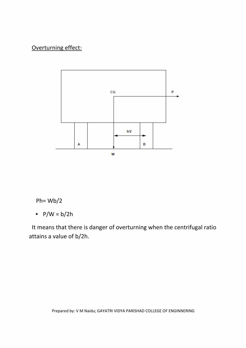
Overturning effect:
Ph= Wb/2
• P/W = b/2h
It means that there is danger of overturning when the centrifugal ratio
attains a value of b/2h.

Prepared by: V M Naidu; GAYATRI VIDYA PARISHAD COLLEGE OF ENGINNERING
Transverse skidding effect:
P= fRA + fRB
= f(RA+Rb)
= fW
Super-elevation:-
• It is the transverse slope provided throughout length of horizontal
curve.
• The purpose of super-elevation is to counteract the effect of
centrifugal force and also to reduce overturn (or) skid of the
vehicle.

Prepared by: V M Naidu; GAYATRI VIDYA PARISHAD COLLEGE OF ENGINNERING
tanӨ = e= NL/ML
TanӨ = SinӨ= e= E/B
PcosӨ = WSinӨ + FA+ FB
PCosӨ = WSinӨ + f(RA+RB)
= WSinӨ + f(WCosӨ+PSinӨ)
P(CosӨ-fSinӨ) = WSinӨ+fWCosӨ
Divide by WCosӨ
(P/W)(1-fTanӨ) = TanӨ + f
P/W = ((TanӨ+f)/(1-fTanӨ))
Prepared by: V M Naidu; GAYATRI VIDYA PARISHAD COLLEGE OF ENGINNERING
As Ө is small tanӨ=0
P/W = TanӨ + f
But P/W = V²/gR ( P= mV²/R= WV²/gR)
e+f = V²/gR
e+f = (0.278V)²/9.8R
e+f= V²/127R
If friction is neglected, f=0
e= V²/127R
If super-elevation is not provide, the allowable speed,
e+f= V²/127R
f= V²/127R
V=√127��
Eg:-
The radius of horizontal circular curve is 100m.the design speed is 50
kmph and design coefficient of lateral friction is 0.15
a) Calculate the super-elevation required for full lateral friction.
b) Calculate the coefficient of friction needed if no super-elevation is
provided.
c) Calculate the equilibrium super-elevation if pressure on inner and
outer wheels should be equal.
Sol:-
Prepared by: V M Naidu; GAYATRI VIDYA PARISHAD COLLEGE OF ENGINNERING
a) e + f= V²/127R
e + 0.15 = 50²/ (127*100)
e= 0.047
b) e+ f= V²/127R
0+f= V²/(127*100)= 0.197
c) e= V²/127R= 50²/(127*100) = 0.197
Steps for super-elevation design:-
Step1:- e= (0.75V)² /gR = V²/225R (Super-elevation for 75% of design
speed)
Step2:- Calculated ‘e’ <0.07 provide that ‘e’ value
If e> 0.07 provide e= 0.07 and proceed
Step3:- f= (V²/127R)-0.07
If ‘f’ calculated <0.15 then e=0.07 is safe.
If ‘f’ calculated >0.15 then restrict speed.
Step 4:
e + f = v2 /(127R)
0.07+ 0.15 = Va2/(127R)
Va = √(0.22 * 127R)
Allowable speed, Va = √(27.94R)
Example: Design the rate of superposition for the horizontal highway
curve of radius 500m and speed 100Kmph.
Prepared by: V M Naidu; GAYATRI VIDYA PARISHAD COLLEGE OF ENGINNERING
Sol:- e = V2/(225R)
= 1002/(225*500) = 0.089 >0.07
e+f = V2/(127R)
0.07+f = 1002/(127*500)
f = 0.087 <0.15
so the design is safe.
Example: The design speed of highway is 80Kmph and radius,
R=200m.Check for safety.
Sol: e = V2/(225R)
= 802/(225*200) = 0.142 >0.07
e+f = V2/(127R)
0.07+f = 802/(127*200)
f = 0.18 >0.15
Therefore design not safe
Therefore restrict the the speed
0.07+0.15 = Va/(127*200)
Va = 74.75Kmph.
ATTAINMENT OF SUPERELEVATION:-
a) Elimination of crown of cambered section
b) Rotation of pavement to attain full superelevation

Prepared by: V M Naidu; GAYATRI VIDYA PARISHAD COLLEGE OF ENGINNERING
RADIUS OF HORIZONTAL CURVE:-
e+f = V2/(127R)
R ruling = V2/((e+f)g) V –Ruling design speed
R min = (VӨ)2(127(e+f)) VӨ –Minimum design speed
WIDENING OF PAVEMENT ON HORIZONTAL CURVE:-
Mechanical widening:-
Wm =OC-OA = OB-OA = R2-R1

Prepared by: V M Naidu; GAYATRI VIDYA PARISHAD COLLEGE OF ENGINNERING
∆OAB, OA2 = OB2- BA2
R12
=R22 –l2
But R1=R2 -wm
(R2 -wm)2 = R22 –l2
l2 = wm(2R2 -wm)
wm = l2/(2R2 -wm) ≈ l
2/(2R); wm =nl
2/(2R) n-no.of lanes.
Psychological widening
As per IRC,
wps = V/(9.5√R)
we = wm + wps
we = nl2/(2R) + V/(9.5√R)
Prepared by: V M Naidu; GAYATRI VIDYA PARISHAD COLLEGE OF ENGINNERING
Example: Calculate the extra widening required for a pavement of
within 7m on a horizontal curve of radius 250m if the longest wheel
base of vehicle expected on the road is 7.0m, Design speed 70Kmph.
Sol: we = wm + wps
= nl2/(2R) + V/(9.5√R)
= (2*72)/(2*250) + 70/(9.5√250)
= 0.662m
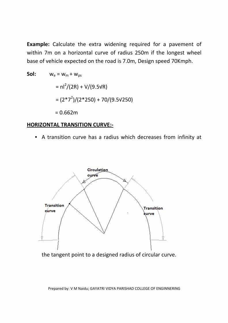
HORIZONTAL TRANSITION CURVE:-
• A transition curve has a radius which decreases from infinity at
the tangent point to a designed radius of circular curve.

Prepared by: V M Naidu; GAYATRI VIDYA PARISHAD COLLEGE OF ENGINNERING
Functions of transition curve:-
a) To introduce gradually the centrifugal force between the
tangent point and the beginning of the circular curve.
b) To enable the driver turn the steering gradually.
c) To enable the gradual introduction of the designed super
elevation and the extra widening.
d) To improve the aesthetic appearance.
Different types of transition curves:
a) Spiral (also called clothoid)
b) Lemniscate
c) Cubic parabola
IRC recommends due to the following reasons:
I. Spiral curve satisfies the requirement of an ideal transition.
II. Geometric property of spiral is such that calculation and setting
out the curve in the field is simple and easy.
Prepared by: V M Naidu; GAYATRI VIDYA PARISHAD COLLEGE OF ENGINNERING
Length of transition, Ls = V3/(CR) = 0.0215V
3/(CR),
V in kmph
Where, C = 80/(75+V)
Ls = EN/2 = eN(w+we)/2 , (for pavement rotating about
centre)
Ls = EN = eN(w+we) , (for pavement rotating about the
inner edge)
Empirical formula:
For plane and rolling terrain:
Ls = 2.7V2/R
For mountainous and steep terrain:
Ls = V2/R
When transition is provided, parallel shift should be provided
S = Ls2/(24R)
Example: Calculate the length of transition curve and shift using
following data:
Design speed = 65Kmph
Radius of circular curve = 220m
Allowable rate of superelevation (about centre line) = 1 in 150
pavement width including extra widening = 7.5m.
Sol- C = 80/(75+V) = 80/(75+65) = 0.57m/s3

Prepared by: V M Naidu; GAYATRI VIDYA PARISHAD COLLEGE OF ENGINNERING
Ls = 0.0215V3/(CR) = 0.021565
3/(0.57*220)=47.1m.......I
e + f = V2/ (127R)
f = 652/ (127*220) – 0.07 = 0.08 < 0.15
Therefore, e= 0.07 is safe
Raise of outer edge = E/2 = eB/2 = (0.07*7.5)/2 = 0.26m
Ls = EN/2 = 0.26*150 =39m..........................................II
Ls = 2.7V2/R = 2.7*652/220 = 51.9m...........................III
Adopt highest, i.e Ls = 51.9 ≈ 52m
Shift, S = Ls2/ (24R) = 522/(24*220) = 0.51m
DESIGN OF VATRICAL ALIGNMENTS:-
• The vertical alignment is the elevation (or) profile of the centre
line of the road.
• Vertical alignment consists of grades and vertical curves.
• Vertical alignment influences the vehicle speed, acceleration,
decelaration, sight distance and comfort.
Gradient:-
• Ruling gradient
• Limiting gradient
• Exceptional gradient
• Minimum gradient
Prepared by: V M Naidu; GAYATRI VIDYA PARISHAD COLLEGE OF ENGINNERING
� Ruling gradient is the maximum gradient within which the designer
attempts to design the vertical profile of the road.
� Limiting gradient is the gradient where the topography of a place
compels adopting steep gradient.
� Exceptional gradient is gradient still steeper than above and it
should be adopted for short stretches.
� Minimum gradation is that gradation, which is provided in view of
drainage and topography. It depends on rainfall, runoff, type of soil,
topography.
GRADE COMPENSATION ON HORIZONTAL CURVES:-
When sharp horizontal curve is to be introduced on a road which
has already the maximum permissible gradation. Then the gradient
should be decreased to compensate for the loss tractive effort due to
the curve.
This reduction n gradation at the horizontal curve is called grade
compensation.
Grade compensation = 30+R/R %
Maximum value = 75/R ‘R’ is radius in m
According to IRC, the grade compensation is not necessary for
gradation flatter than 4.0%.
VERTICAL CURVES:-
Due to change in grade in the vertical alignment of highway, it is
necessary to introduce vertical curves at the intersection of different
grades.
Prepared by: V M Naidu; GAYATRI VIDYA PARISHAD COLLEGE OF ENGINNERING
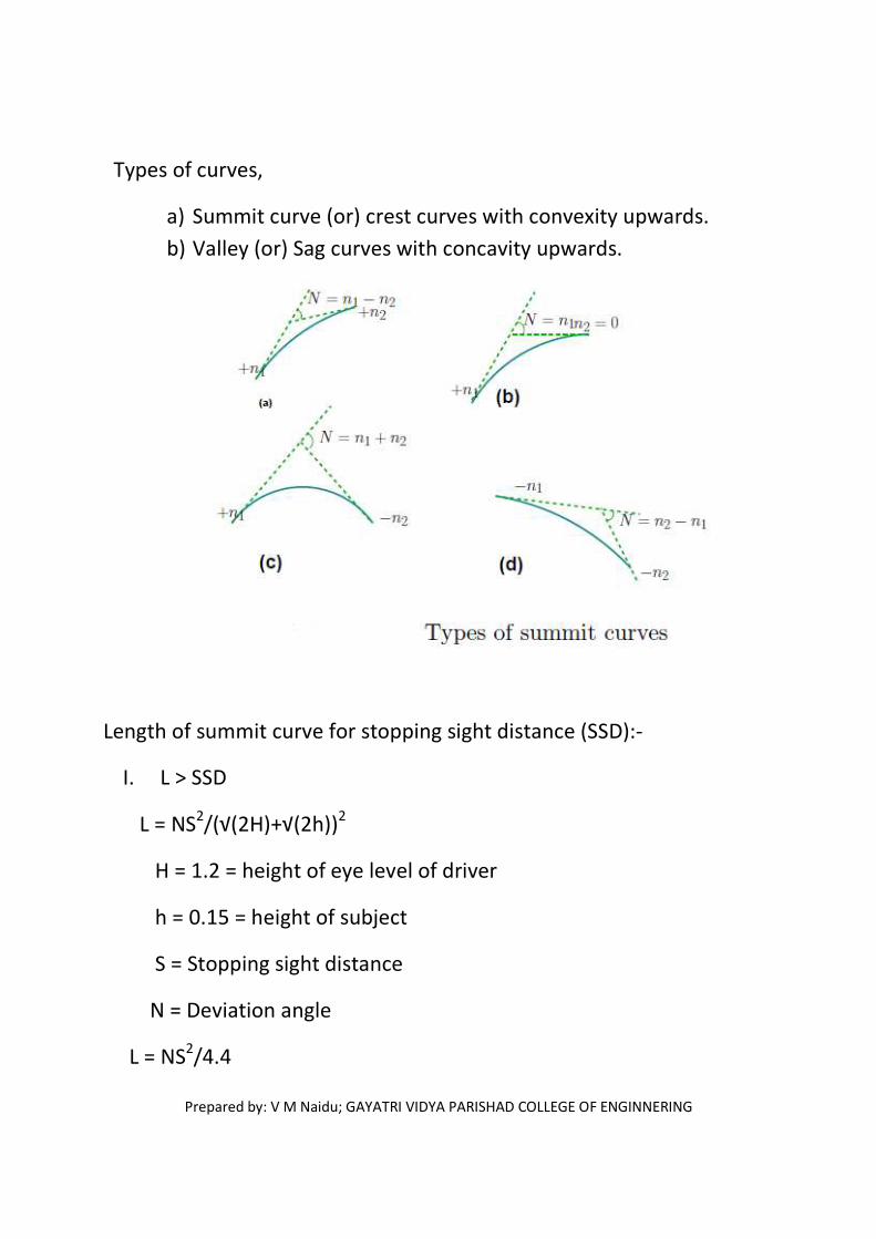
Types of curves,
a) Summit curve (or) crest curves with convexity upwards.
b) Valley (or) Sag curves with concavity upwards.
Length of summit curve for stopping sight distance (SSD):-
I. L > SSD
L = NS2/(√(2H)+√(2h))2
H = 1.2 = height of eye level of driver
h = 0.15 = height of subject
S = Stopping sight distance
N = Deviation angle
L = NS2/4.4

Prepared by: V M Naidu; GAYATRI VIDYA PARISHAD COLLEGE OF ENGINNERING
II. L < SSD
L= 2S -(√(2H)+√(2h))2/N
L = 2S – 4.4/N
LENGTH OF SUMIT CURVE FOR OVERTAKING SIGHT SIGHT DISTANCE
(or) INTERMEDIATE SIGHT DIASTANCE:-
i. L > OSD
L = NS2/(8H)
L = NS2/(9.6)
ii. L < OSD
L= 2S-8H/N
L= 2S-8H/N
VALLEY CURVES:-

Prepared by: V M Naidu; GAYATRI VIDYA PARISHAD COLLEGE OF ENGINNERING
1) Comfort condition
L = 2(NV3/C)1/2 V is in m/s
2) Length of valley curve for head light sight distance
i. L > SSD
L = NS2/(2h1+2Stanα)
L = NS2/(1.5+0.035S)
ii. L < SSD
L = 2S-(2h1+2Stanα)/N
L = 2S-(1.5+0.035S)/N

Prepared by: V M Naidu; GAYATRI VIDYA PARISHAD COLLEGE OF ENGINNERING
Example: A vertical summit curve is formed at the intersection of
gradients +3.0% and -5.0%. Design the length of summit curve to
provide a stopping sight distance for a design speed of 80Kmph.
Assume other data.
Sol:-
a) SSD = 0.278Vt + (V2/254f) assume t= 2.5sec, f= 0.35
= 0.278*80*2.5 + (802/(254*0.35)) = 128m
b) Deviation angle = 0.03- (-0.05) = 0.08
Assume L> SSD
L= (NS2/4.4) = (0.08*1282)/4.4 = 297.8 (128m)
L= 298m
Ex:-
An ascending gradient of 1 in 100 meets a descending gradient of 1 in
120. A summit curve is to be designed for a speed of 80 kmph so as to
have an overtaking sight distance of 470m.
Sol:-
n1= 1/100, n2= -1/120
N= (1/100)-(-1/120)= 11/600
Assume L> OSD
L= (NS2/9.6) = (11/600)*(470
2/9.6) = 422 (<470)
L<OSD should be considered

Prepared by: V M Naidu; GAYATRI VIDYA PARISHAD COLLEGE OF ENGINNERING
L=2S-(9.6/N)
= (2*470)-(9.6/(11/600))
= 416.4m (<470m)
Length of summit curve = 417m.
Ex:
A valley curve is formed by a descending grade of 1 in 25 meeting on
ascending grade of 1 in 30.Design the length of valley curve to fulfill
both comfort condition and head light sight distance requirements.
Assume c=0.6m/S3, t= 2.5 sec; f= 0.35?
Sol:-
N = - (1/25) - (1/30) = -11/150
V= 80 kmph = 80/3.6 = 22.2 m/s
a) Comfort condition
L= 2*(NV3/C)1/2 = 2*(11*22.23/(150*0.6))1/2 = 73.1m
b) Head light sight distance
T=2.5 sec, f=0.35
SSD = Vt + (V2/2gf) = 127.3m
If L>SSD
L= (NS2/(1.5+0.0355)) = (11*127.32/(150(1.5+(0.0035*127.3))))
= 199.5 (<127.3)
Length of valley curve

Prepared by: V M Naidu; GAYATRI VIDYA PARISHAD COLLEGE OF ENGINNERING
= 199.5m
= 200m

Prepared by: V M Naidu; GAYATRI VIDYA PARISHAD COLLEGE OF ENGINNERING
UNIT-5
TRAFFIC ENGINEERING
It is that branch of engineering which deals with deals with the
improvement of traffic performance of road networks and terminals.
It is achieved by systematic traffic studies, scientific analysis and
engineering application.
SCOPE OF TRAFFIC ENGINEERING:
The objective of traffic engineering is to achieve efficient, free and
rapid flow of traffic with minimum number of accidents.
The study of traffic engineering is divided into following major
sections:
1) Traffic characteristics.
2) Traffic studies and analysis.
3) Traffic operation-control and regulation.
4) Planning and analysis.
5) Geometric design
6) Administration and management.
TRAFFIC CHARACTERISTICS
Road user characteristics a) Physical(vision, hearing)

Prepared by: V M Naidu; GAYATRI VIDYA PARISHAD COLLEGE OF ENGINNERING
b) Mental(knowledge, skill,
intelligence)
Vehicular characteristics
a) Vehicle dimensions
b) Wt. of loaded vehicle.
c) Power of vehicle.

Prepared by: V M Naidu; GAYATRI VIDYA PARISHAD COLLEGE OF ENGINNERING
c) Psychological(fear, anger, d) Speed of vehicle
maturity) e) Braking characteristics
d) Environmental.
Example:
In a braking test, a vehicle travelling at a speed of
30Kmph.Was stopped by applying brakes fully and the skid marks were
5.8m in length. Determine the average skid resistance of the pavement
surface.
Sol:
Initial speed, U=30Kmph = (30/3.6)m/s = 8.33 m/s.
Braking distance, L= 5.8m = (U2/2gf)
5.8 = (8.332/2*9.81*f)
f = (8.332/2*9.81*5.8)
Avg skid, f= 0.61
Example:
A vehicle travelling at 40Kmph was stopped within 1.8sec after the
application of the brakes. Determine the average skid resistance.
Sol:
F=ma = fW
(W/g*a) = fW

Prepared by: V M Naidu; GAYATRI VIDYA PARISHAD COLLEGE OF ENGINNERING
f= (a/g)
a= (u/t) = (40/3.6/1.8) = 6.17m/s2.
f= a/g = 6.17/9.81 = 0.63.
Example:
A vehicle was stopped in 1.4 sec by fully jamming the brakes and
the skid marks measured 7.0m. Determine average skid resistance.
Sol:
V= u +at
0 = u + at => u= -at
V2-U2 = 2as => 0 – U2 = 2as => a2t2 = 2as
a = (2S/t2) = 2(7/1.4
2)
f= a/g = (2*7/1.42*9.81) = 0.73
VOLUME-SPEED-DENSITY RELATION:
Volume of traffic is the no. of vehicles passing a particular
section in unit time.
Speed is the distance travelled by the no. of vehicles in unit
time.
Density of traffic is the no. of vehicles plying in unit length of
highway.

Prepared by: V M Naidu; GAYATRI VIDYA PARISHAD COLLEGE OF ENGINNERING
As speed increased, volume increases upon maximum value and
then decreases.
Similarly, as the density of traffic plying on the road increases,
volume increases upto maximum value and then decreases.
The maximum speed value in the figure is called free mean
speed, Vsf
The maximum density at zero speed is called jam density, kj
The maximum flow or capacity flow, qmax occurs when the speed
is Vsf/2 and density is Kj/2.
Qmax = (Vsf/2)*(Kj/2) = (VsfKj/4).
Prepared by: V M Naidu; GAYATRI VIDYA PARISHAD COLLEGE OF ENGINNERING
Example:
The free mean speed on roadway is found to be 80Kmph. Under
stopped condition the average spacing between the vehicles is 6.9m.
determine the capacity flow.
Sol:
Free mean speed, Vsf = 80Kmph
Jam velocity, Kj= 1000/6.9 = 145veh/km/lane
Max flow, qmax= (80*145/4)= 2900 vehicles/hr/lane.
TRAFFIC VOLUME STUDY:
• Traffic volume is the number of vehicles crossing a section of road
per unit time at any selected period.
• A complete traffic volume study may include the classified volume
study by recording the volume of various vehicle types.
Objects and uses of traffic volume studies:
• Traffic volume is generally accepted as a true measure of the
relative importance of roads.
• Used in deciding properties for improvement and expansion.
• It is used in planning and designing of new facilities.
• It is used in analysis of traffic pattern and trends.
• Classified volume study is useful in structural design of
pavements, in geometric design and in computing roadway
capacity.
• It is used in planning one-way streets.
Prepared by: V M Naidu; GAYATRI VIDYA PARISHAD COLLEGE OF ENGINNERING
• Turning movement study is used in design of intersection.
• Pedestrian traffic study is used planning of side walk, cross walk
and pedestrian signal.

Prepared by: V M Naidu; GAYATRI VIDYA PARISHAD COLLEGE OF ENGINNERING
Classified volume count format:-
Two
wheeler
Car/
jeep/
van
Auto Bus LCV 2-
Axle
Truck
3-
Axle
Truck
Multi
axle
truck
Cycle Others
Counting of traffic volume:-
Mechanical counters:-
• These are either fixed (permanent) type (or) portable type.
• These can automatically record the total number of vehicles
crossing a section of road in desired period.
• Traffic count is recorded by electrically operated counters and
recorders capable of recording the impulses.
• Examples of mechanical detectors are by photo-electric cells,
magnetic detector and radar detectors.
Prepared by: V M Naidu; GAYATRI VIDYA PARISHAD COLLEGE OF ENGINNERING
• The main advantage of mechanical counter is that it can work
throughout the day and night for the desired period. And,
recording of hourly volume, is not predictable by manual
counting.
• The main drawback of mechanical counter is that it is not
possible to get the traffic volume of various classes and details
of turning movement.
Manual counts:-
a) This method employs a field team to record traffic volume on the
prescribed record sheets.
b) This method is useful where mechanical counting methods are not
useful. For example, vehicle classification, turning movement
details cannot be gathered by mechanical counters.
Presentation of traffic volume data:-
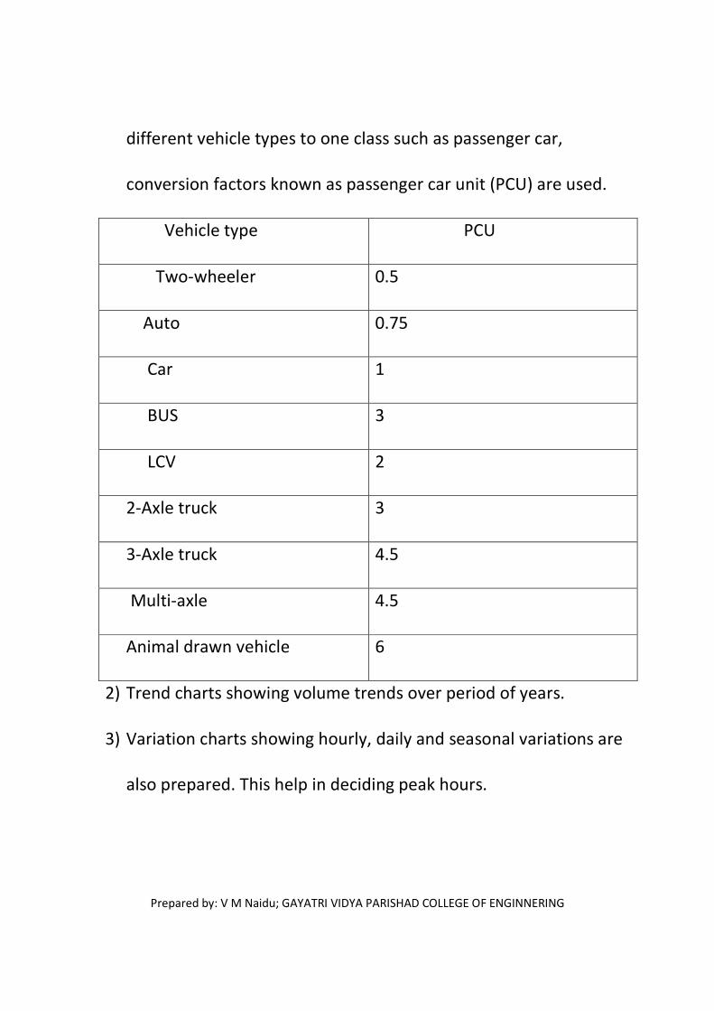
1) Annual average daily traffic (AADT or ADT) of the total traffic as
well as classified traffic are calculated. In order to convert
Prepared by: V M Naidu; GAYATRI VIDYA PARISHAD COLLEGE OF ENGINNERING
different vehicle types to one class such as passenger car,
conversion factors known as passenger car unit (PCU) are used.
Vehicle type PCU
Two-wheeler 0.5
Auto 0.75
Car 1
BUS 3
LCV 2
2-Axle truck 3
3-Axle truck 4.5
Multi-axle 4.5
Animal drawn vehicle 6
2) Trend charts showing volume trends over period of years.
3) Variation charts showing hourly, daily and seasonal variations are
also prepared. This help in deciding peak hours.

Prepared by: V M Naidu; GAYATRI VIDYA PARISHAD COLLEGE OF ENGINNERING
4) Traffic flow maps along the routes, (the thickness of the lines
representing the traffic volume to any desired scale) are drawn.
These help to find the traffic volume distribution.
5) Volume floe diagram at intersections either drawn to a certain
scale or indicating traffic volume.
Prepared by: V M Naidu; GAYATRI VIDYA PARISHAD COLLEGE OF ENGINNERING
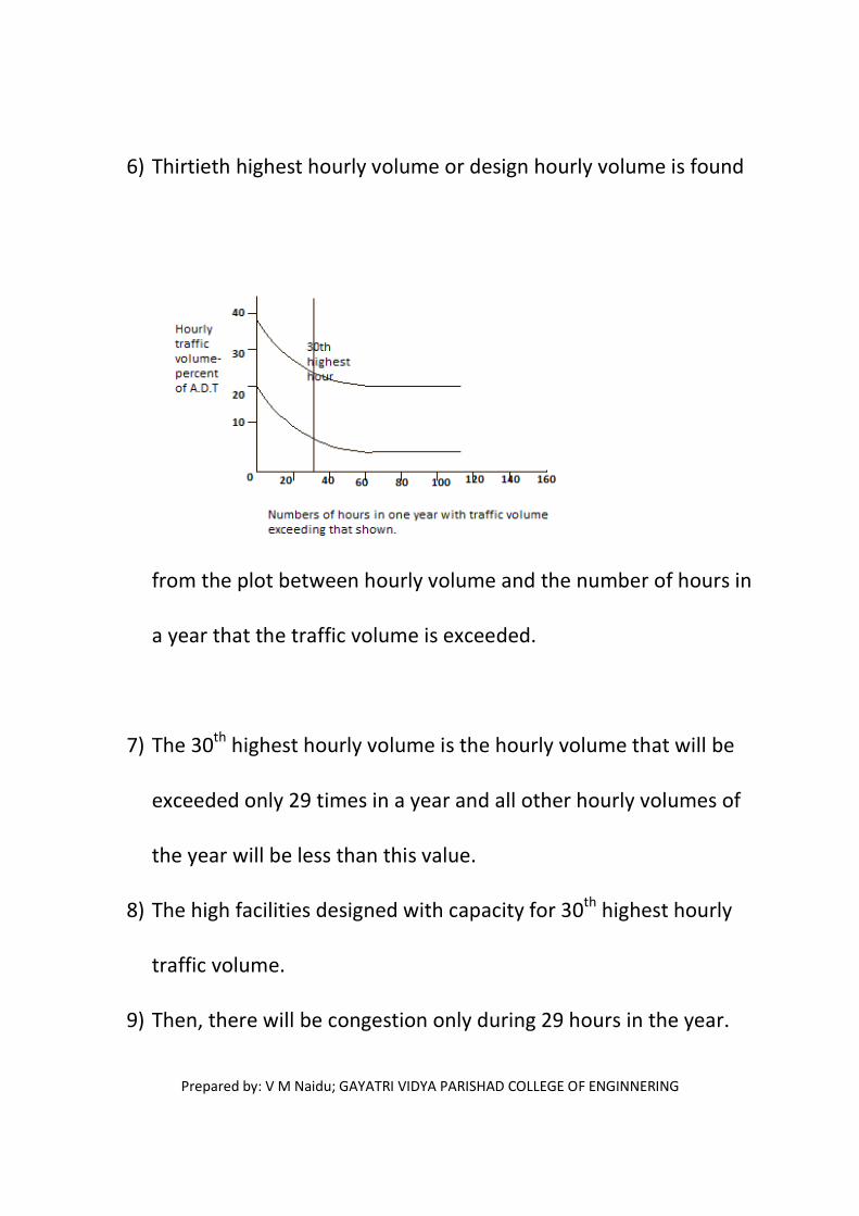
6) Thirtieth highest hourly volume or design hourly volume is found
from the plot between hourly volume and the number of hours in
a year that the traffic volume is exceeded.
7) The 30th highest hourly volume is the hourly volume that will be
exceeded only 29 times in a year and all other hourly volumes of
the year will be less than this value.
8) The high facilities designed with capacity for 30th highest hourly
traffic volume.
9) Then, there will be congestion only during 29 hours in the year.

Prepared by: V M Naidu; GAYATRI VIDYA PARISHAD COLLEGE OF ENGINNERING
10) The 30th
highest hourly volume is generally taken as the
hourly volume for design.
Speed studies:-
• Actual speed of vehicle over a particular route may vary
depending on several factors such as geometric features,
traffic condition, time, place, environment and drive.
• Travel time is reciprocal of speed and it also gives operating
condition of road network.
• Spot speed is the instantaneous speed of a vehicle at a
specified section.
• Average speed is the average of the spot speeds of all vehicles
passing a given point on the road.
Average Speed
Space-mean speed Time-mean speed

Prepared by: V M Naidu; GAYATRI VIDYA PARISHAD COLLEGE OF ENGINNERING
• Space-mean speed represents the average speed of vehicles in
a certain road length at any time.
• This (Space-mean speed) is obtained from the observed travel
time of vehicles over relatively long stretch of the road.
Space-mean speed is calculated from:-
Vs=3.6dn/(∑ ����� ��
)
Where Vs= space-mean speed, Kmph
D= length of the road.
N= number of individual vehicle observations.
Ti= observed travel time(sec) for ith
vehicle to travel
distanced, m
• The average travel time of all vehicles is obtained from the
reciprocal of space-mean speed.
• Time-mean speed represents the speed distribution of
vehicles at a point on roadway.
Prepared by: V M Naidu; GAYATRI VIDYA PARISHAD COLLEGE OF ENGINNERING
• Time-mean speed is the average of instantaneous speeds of
observed vehicles at the spot.
Time-mean speed is calculated from:-
Vt= (∑ ����� ��
)
Where Vt= time-mean speed.
Vi= observed instantaneous speed of ith
vehicles Kmph.
N= no. of observed vehicles.
• Under typical speed conditions.
Vs< Vt
• Running speed=(Distance covered/Running time)
Running time=total time-stopped delay
• Overall speed or travel speed is the effective speed with which
a vehicle traverses a particular route between two terminals
Overall speed= (Total distance/Total time)
Total time (including all delays and stoppages)
• There two types of speed studies.

Prepared by: V M Naidu; GAYATRI VIDYA PARISHAD COLLEGE OF ENGINNERING
i. Spot speed study.
ii. Speed and delay study.
Spot speed study:-
It is useful in any of the following aspects of traffic engineering:
a) To use in planning traffic control.
b) To use in geometric design.
c) To use in accident studies.
d) To study traffic capacity.
e) To decide speed trends.
f) To compare diverse types of drivers.
The spot speeds are affected by physical features of the road like
pavement width, curve, sight distance, gradient, pavement
unevenness, intersection and road side development.

Prepared by: V M Naidu; GAYATRI VIDYA PARISHAD COLLEGE OF ENGINNERING
Other factors affecting spot speeds are environment conditions,
enforcement, traffic conditions.
Enoscope is used to find the spot speeds of vehicles.
Other equipment used for speed measurement are graphic
recorder, electronic meter, photo electric meter, radar, speed
meter and by photographic methods.]
Out of all these, the radar speed meter method seems to be the
most efficient one as it captures speeds instantaneously.
Presentation of spot speed data:-
a) Average speed of vehicles

Prepared by: V M Naidu; GAYATRI VIDYA PARISHAD COLLEGE OF ENGINNERING
• The arithmetic mean is taken as the average speed.
b) Cumulative speed of vehicles.
15% speed ---> lower limit speed.
50% speed -� average speed.
85% speed -� upper limit speed.
98% speed -� design speed.
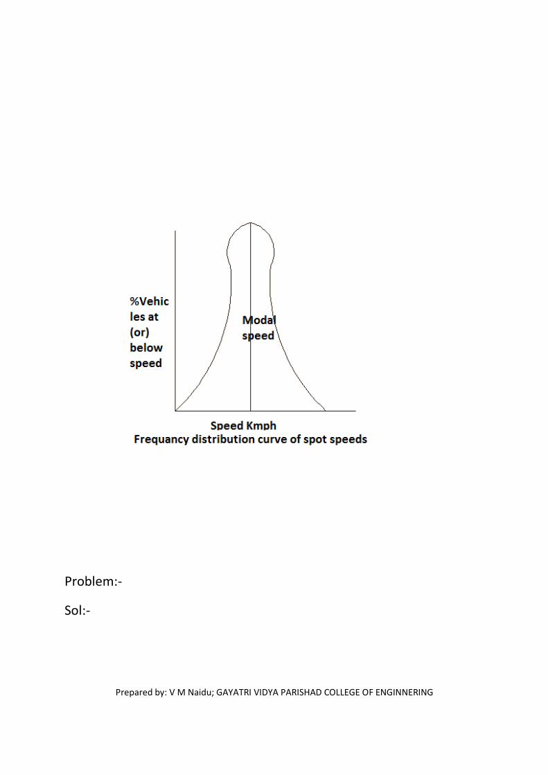
c) Modal average
Prepared by: V M Naidu; GAYATRI VIDYA PARISHAD COLLEGE OF ENGINNERING
Problem:-
Sol:-

Prepared by: V M Naidu; GAYATRI VIDYA PARISHAD COLLEGE OF ENGINNERING
Speed range Mid speed Frequency Frequency% Cumulative
frequency
(%)
0-10 5 12 1.4 1.4
10-20 15 18 2.1 3.53
20-30 25 68 8.0 11.53
30-40 35 89 10.47 22.00
40-50 45 204 24 46.00
50-60 55 255 30 76.00
60-70 65 119 14 90.00
70-80 75 43 5 95.00
80-90 85 33 3.88 98.94
90-100 95 9 1.06 100.00
From graph
i. Upper speed limit for regulation=85 percentile speed= 60 Kmph
ii. Lower speed limit for regulation=15 percentile speed= 30 Kmph
iii. Speed to check design elements =95 percentile speed= 84 Kmph
Speed and delay study:-
• This study gives the running speeds, overall speeds,
fluctuations in speed and the delay between stations.
There are various methods of carrying out speed and delay study,
namely:-
a) Floating car method.
b) License plate method.

Prepared by: V M Naidu; GAYATRI VIDYA PARISHAD COLLEGE OF ENGINNERING
c) Interview technique.
d) Elevated observation.
e) Photographic technique.
The average journey time t (minute)
T̀=tw-ny/q
Q= (na+ny) / (ta+tw)
Where q= flow of vehicles (volume per min) in one direction of the
stream.
Na=average no. of vehicles counted in the direction of stream
when the test vehicle travels in opposite direction.
Ny= {average no. of overtaking}-{no. of overtaken vehicles}
Tw=average journey time, in minutes, vehicle travelling
against stream, q
Ta= average journey time, in minutes, vehicle travelling
against stream, q

Prepared by: V M Naidu; GAYATRI VIDYA PARISHAD COLLEGE OF ENGINNERING
Problem:-
Stretch length= 3.5Km.
Trip
no.
Direction
of trip
Journey
time
Min.sec
Total
stopped
delay
min.sec
No. of
veh.
overtaking
No. of
vehicles
overtaken
No. of
veh.
From
opp.
direction
1 N-S 6-32 1-40 4 7 268
2 S-N 7-14 1-50 5 3 186
3 N-S 6-50 1-30 5 3 280
4 S-N 7-40 2-00 2 1 200
5 N-S 6-10 1-10 3 5 250
6 S-N 8-00 2-22 2 2 170
7 N-S 6-28 1-40 2 5 290
8 S-N 7-30 1-40 3 2 160
Sol:-
Direction Journey
time
Stopped
delay
Overtaking Overtaken In opp.
Direction
N-S 6-32 1-40 4 7 268
6-50 1-30 5 3 280
6-10 1-10 3 5 250
6-28 1-40 2 5 290
Total: 26-00 6-00 14 20 1088
Mean: 6-30 1-30 3.5 5.0 272
S-N 7-14 1-50 5 3 186
7-40 2-00 2 1 200
8-00 2-22 2 2 170
7-30 1-40 3 2 160
Total: 30-24 7-12 12 8 716
Mean: 7-36 1-46 3 2 179
Prepared by: V M Naidu; GAYATRI VIDYA PARISHAD COLLEGE OF ENGINNERING
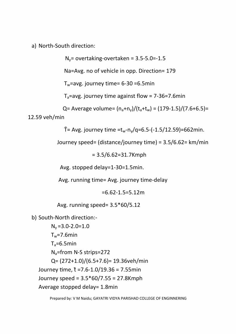
a) North-South direction:
Ny= overtaking-overtaken = 3.5-5.0=-1.5
Na=Avg. no of vehicle in opp. Direction= 179
Tw=avg. journey time= 6-30 =6.5min
Ta=avg. journey time against flow = 7-36=7.6min
Q= Average volume= (na+ny)/(ta+tw) = (179-1.5)/(7.6+6.5)=
12.59 veh/min
T̀= Avg. journey time =tw-ny/q=6.5-(-1.5/12.59)=662min.
Journey speed= (distance/journey time) = 3.5/6.62= km/min
= 3.5/6.62=31.7Kmph
Avg. stopped delay=1-30=1.5min.
Avg. running time= Avg. journey time-delay
=6.62-1.5=5.12m
Avg. running speed= 3.5*60/5.12
b) South-North direction:-
Ny =3.0-2.0=1.0
Tw=7.6min
Ta=6.5min
Na=from N-S strips=272
Q= (272+1.0)/(6.5+7.6)= 19.36veh/min
Journey cme, t̄̄ =7.6-1.0/19.36 = 7.55min
Journey speed = 3.5*60/7.55 = 27.8Kmph
Average stopped delay= 1.8min

Prepared by: V M Naidu; GAYATRI VIDYA PARISHAD COLLEGE OF ENGINNERING
Average running time = 7.55-1.80 = 5.75min
Average running speed=3.5*60/5.75= 36.5Kmph
Parking studies:
• Parking space is one of the major problems in
transportation.
• Parking demand is high in industrial, commercial and
residential places.
• Parking studies are useful to evaluate the parking
facilities.
Parking demand:-
• Parking demand may be evaluated by different methods.
Method1:-
Cordon counts are conducted to study parking
accumulation in the study area.
Method2:
By noting the registration number of each parked vehicle
at any desired time interval (such as 1/2hr, 1hr etc).
Parking characteristics:-

Prepared by: V M Naidu; GAYATRI VIDYA PARISHAD COLLEGE OF ENGINNERING
• The study is directed to note the present parking
practices prevalent in study area and the general
problems in parking.
Parking space inventory:-
• The study area is fully surveyed and a map is prepared
showing kerb parking (on-street parking) and off-street
parking to meet parking demands.
Accident studies:-
• Due to complex flow patterns, mixed traffic condition,
the accident problems are increasing.
• Traffic accidents involves property damage, minor injury,
fatal.
• With suitable traffic engineering, accident rate cannot be
eliminated but can be decreased.
Objectives of accident studies:-
a) To study the causes of accidents.
b) To evaluate existing designs.
c) To support proposed designs.
d) To carry out before and after studies.
e) To make computations of financial loss.
f) To give economic justification for the improvements.
Causes of accidents:-
• Drivers.
• Pedestrians.
• Passengers.

Prepared by: V M Naidu; GAYATRI VIDYA PARISHAD COLLEGE OF ENGINNERING
• Vehicle defects.
• Road condition.
• Road design.
• Weather.
• Animals.
Preventive measures of road accidents;-
Accident rate can be reduced by following three groups. (3-E’s)
a) Engineering.
b) Enforcement.
c) Education.
Engineering measures:-
a) Road design.
b) Maintenance of vehicle.
c) Before and after studies.
d) Road lighting.
Enforcement measures:-
a) Speed control.
b) Traffic control devices.
c) Training and supervision.
d) Medical check.
e) Special precautions for commercial vehicles.
Educational measures:-

Prepared by: V M Naidu; GAYATRI VIDYA PARISHAD COLLEGE OF ENGINNERING
a) Education of road users.
b) Safety week.
Accident recording:-
• Collecting of accident data
a) General (date, time, etc)
b) Location.
c) Details of vehicles involved.
d) Nature of accident.
e) Road and traffic conditions.
f) Primary causes of accident.
• Accident report
• Accident records
a) Location files.
b) Spot maps.

Prepared by: V M Naidu; GAYATRI VIDYA PARISHAD COLLEGE OF ENGINNERING
Condition diagram:-
It is a scaled drawing showing all important physical conditions of
an accident location.
The physical conditions are roadway limits, curves, bridges, culverts,
trees, signs, signals etc.
Condition diagram of 4-legged jn
Collision diagram:-
It is a drawing showing the paths of vehicles and pedestrians
involved in the accidents.
It is useful to compare accident pattern before and after the
remedial measures
Typical collision diagram and symbols:-
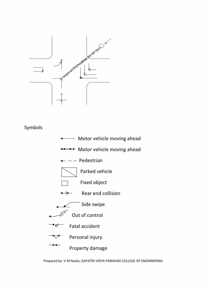
Prepared by: V M Naidu; GAYATRI VIDYA PARISHAD COLLEGE OF ENGINNERING
Symbols
Motor vehicle moving ahead
Motor vehicle moving ahead
Pedestrian
Parked vehicle
Fixed object
Rear end collision
Side swipe
Out of control
Fatal accident
Personal injury
Property damage

Prepared by: V M Naidu; GAYATRI VIDYA PARISHAD COLLEGE OF ENGINNERING
UNIT-6
TRAFFIC REGULATION AND MANAGEMENT
Traffic signs:-
According to motor vehicle act, traffic signs are divided into three
categories.
a) Regulatory signs.
b) Warning signs.
c) Informatory signs.

Prepared by: V M Naidu; GAYATRI VIDYA PARISHAD COLLEGE OF ENGINNERING
Placement of sign board:-
• Size, shape, colour code should be provided as per the
IRC(Indian Road Congress)
• The reverse side of all the sign plates should be painted grey.
Regulatory signs:- (Mandatory signs)
• These are meant to inform the road users of certain laws,
regulations and prohibitions.
• Violation of these signs are legal offence.
Regulatory Signs
1) Stop and give-away signs.
2) Prohibitory signs.
3) no parking and no stopping signs.
4) Speed limit and vehicle control signs.
5) Restriction end signs.
6) Compulsory direction control.
Stop sign:-
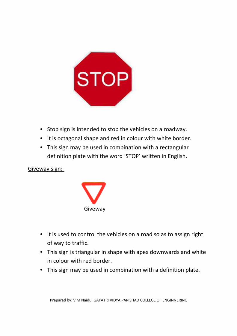
Prepared by: V M Naidu; GAYATRI VIDYA PARISHAD COLLEGE OF ENGINNERING
• Stop sign is intended to stop the vehicles on a roadway.
• It is octagonal shape and red in colour with white border.
• This sign may be used in combination with a rectangular
definition plate with the word ‘STOP’ written in English.
Giveway sign:-
Giveway
• It is used to control the vehicles on a road so as to assign right
of way to traffic.
• This sign is triangular in shape with apex downwards and white
in colour with red border.
• This sign may be used in combination with a definition plate.

Prepared by: V M Naidu; GAYATRI VIDYA PARISHAD COLLEGE OF ENGINNERING
Prohibitory signs:-
No Straight way 600mm No Left
One-way
No right
• These are meant to prohibit certain traffic movements, use of
horns (or) entry of certain vehicle type.
• These are circular in shape and white in colour with a red
border.
No parking sign:-

Prepared by: V M Naidu; GAYATRI VIDYA PARISHAD COLLEGE OF ENGINNERING
• It is meant to prohibit parking of vehicles at that place.
• Definition plate may be indicated.
• It is circular shape with a blue back ground, a red border and an
oblique red bar at an angle 45˚.
No stopping and Standing sign:-
• It is meant to prohibit stopping of vehicles at that place.
• It is circular in shape with blue back ground and two oblique red
bars at 45˚ at right angle.
Speed limit sign:-
• It is meant to restrict the speed of all vehicle on that stretch.
• These are circular shape, white background, red border and
black numerals.
Restriction end sign:-
Prepared by: V M Naidu; GAYATRI VIDYA PARISHAD COLLEGE OF ENGINNERING
• Prohibitions notified is cease to apply after seeing it.
• These signs are also circular with a white back ground and a
broad diagonal black bond at 45˚.
Warning signs:- (cautionary signs)
• These are used to warn the road users of certain hazardous
conditions that exist on (or) adjacent to the roadway.
• The warning signs are in the shape of equilateral triangle with
its apex pointing upwards.
• They are white background, red border and black symbols.
• These are located in advance at a distance of
120m ----> NH/SH
90m ----> MDR
60m ----> ODR
40m ----> VR
On urban roads, this distance is 50m

Prepared by: V M Naidu; GAYATRI VIDYA PARISHAD COLLEGE OF ENGINNERING
Informatory signs:-
• These are used to guide the road users along the route.
• It informs the destination, distance and provide travel easier,
safe and pleasant.
• The direction and place identification signs are rectangular with
white background, black border and black arrows and letters.
• Facility (i.e., Telephone, petrol pump, hospital) information
signs are rectangular with blue back ground and white/black
letters/symbols.
Traffic signal:-
• At intersection where there are large no. of crossings and right
turn traffic, it requires traffic control.
• Earlier, traffic control is carried by traffic police.
• Traffic signal is alternative device to control traffic at
intersections.
Prepared by: V M Naidu; GAYATRI VIDYA PARISHAD COLLEGE OF ENGINNERING
Advantages of traffic signals:-
1) They provide already movement of traffic and increase handling
capacity.
2) They reduce certain type of accidents.
3) Pedestrian can cross road safely.
4) Heavy traffic flow cross intersection safely.
5) Reasonable speed can be maintained.
6) Works economically, when compared to manual control.
7) Quality of traffic flow improved by forming platoons.
Disadvantages of traffic signal:-
1) The rear-end collisions may increase.
2) Improper design and location leads to violations.
3) Failure of signal due to electric power failure cause confusion to
the road user.
Terminology:-
� Cycle:-
The period of time required for one complete sequence of
signal indication is called cycle.
� Phase:-
A part of the signal cycle allocated to a traffic movement (or)
combination of traffic movements is called phase.
Types of traffic signals:-
a) Traffic control signals
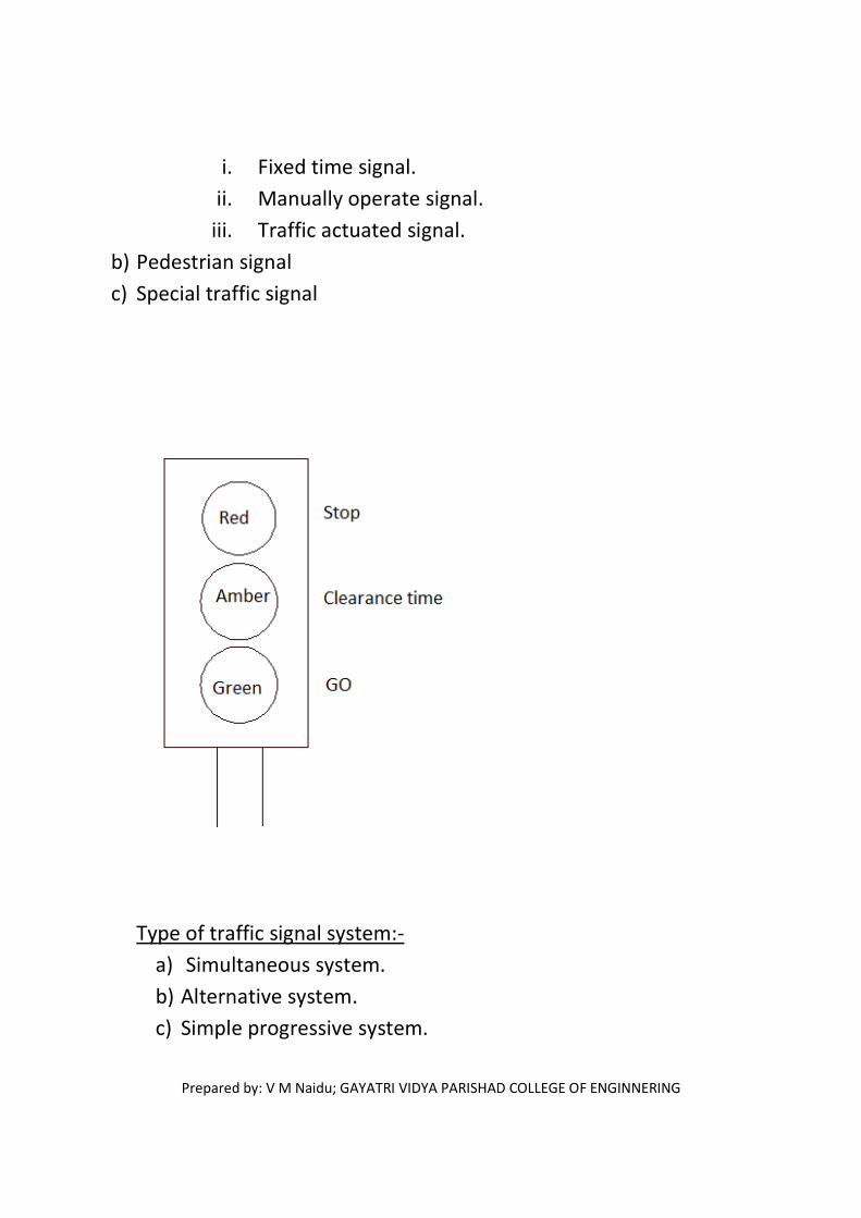
Prepared by: V M Naidu; GAYATRI VIDYA PARISHAD COLLEGE OF ENGINNERING
i. Fixed time signal.
ii. Manually operate signal.
iii. Traffic actuated signal.
b) Pedestrian signal
c) Special traffic signal
Type of traffic signal system:-
a) Simultaneous system.
b) Alternative system.
c) Simple progressive system.

Prepared by: V M Naidu; GAYATRI VIDYA PARISHAD COLLEGE OF ENGINNERING
d) Flexible progressive system.
Warrants for traffic control signal:-
Traffic signal should not be installed unless one (or) more of the
following signal warrants are met.
• When 5 (or) more accidents occurred within 12 months period
at a junction, the signal installation is preferred.
Webster’s method:-
• This is the method used to design the traffic signal.

Prepared by: V M Naidu; GAYATRI VIDYA PARISHAD COLLEGE OF ENGINNERING
Ratio, y1=q1/s1
Y2=q2/s2
q1, q2 are normal flows veh/hr.
s1, s2 are saturation flow veh/hr.
The optimum signal cycle is given by:
C0= (1.5L+5) /1-Y
Y= y1+y2; L=2n+R
N= no. of phases.
R= All red time.
Then, G1= y1(C0-L)/Y and G2= y2(C0-L)/Y
Example:-
The average normal flow of traffic on cross roads A and B during design
period are 400 and 250PCU/hr, the saturation flow values on these
roads are estimated as 1250 and 1000 PCU/hr respectively. The all red
time require for pedestrian crossing is 12 sec. design two phase traffic
signal by webster’s method.
Sol:-
ya= qa/sa
yb= qb/sb
Y=ya +yb = 0.32+0.25=0.57
L=2n+R = 2*2+12 = 16

Prepared by: V M Naidu; GAYATRI VIDYA PARISHAD COLLEGE OF ENGINNERING
Optimum cycle length,
C0= (1.5L+5) /1-Y
= (1.5*16+5) /(1-0.57)
= 67.4sec = 67.5
Ga= ya(C0-L)/Y = 0.32(67.5-16)/0.57 = 29sec
Gb= yb(C0-L)/Y = 0.25(67.5-16)/0.57= 22.5sec
All red time =12sec.
Provide Amber time = 2 sec.
Total cycle time= 29+22.5+12+4 = 67.5sec
IRC METHOD:-
Step:-1 The pedestrian green time required for major and minor roads
are calculate based on walking speed of 1.2m/s and initial walking time
7.0 sec.
Step:-2The green time required for the vehicular traffic on the major
road is increased in proportion to the traffic on two approach.
Step:-3 The cycle time is calculated after allowing amber time of
2.0secs each.
Step:-4 The minimum green time required for clearing vehicles during
the cycle is determined for each lane of approach road assuming the
first vehicle will take 60secs and subsequent vehicle of the queue will
be cleared at the rate of 2.0secs.

Prepared by: V M Naidu; GAYATRI VIDYA PARISHAD COLLEGE OF ENGINNERING
Step:-5 The optimum signal cycle length/time is calculated using
Webster formulae.
Road width Saturation flow
3.0m 1850Pcu/hr
3.5m 1890
4.0m 1950
4.5m 2250
5.0m 2550
5.5m 2990
Step:-6 The signal cycle time and phases may be revised keeping in
view the green time required for clearing the vehicles.
Road Marking:-
• Road marking are made of lines, patterns, words, symbols on
the pavement, kerb, sides of island.
• These are to control, warn, guide (or) regulate the traffic.
• Light reflecting points are commonly used for traffic marking for
night visibility.
• In order to ensure that the markings are seen by the road users,
the longitudinal lines should be atleast 10cm thick.
The various types of markings may be classified as:
a) Pavement markings.
b) Kerb markings.
c) Object markings.
d) Reflector unit markings.
Pavement markings:-

Prepared by: V M Naidu; GAYATRI VIDYA PARISHAD COLLEGE OF ENGINNERING
• It may be of white paint.
• Yellow colour markings are used to indicate parking restriction
and for continuous centre line and barrier line.
1) Centre lines:-
NH, SH 4.5 7.5
OTHER ROADS 3.0 6.0
URBAN ROADS 3.0 4.5
2) Lane lines:-
• Lines are drawn to designate traffic lane.
• These are used to guide the traffic and to properly utilize the
carriageway.
3) No passing zone marking:-
• These are marked to indicate that overtaking is not permitted.
4) Turn markings.
5) Stop lines.
6) Cross walk lines.
7) Approach to obstruction.
8) Parking space limits.
9) Border (or) edge lines.
10) Route direction arrows.
11) Bus stops.
Kerb marking:-

Prepared by: V M Naidu; GAYATRI VIDYA PARISHAD COLLEGE OF ENGINNERING
• These may indicate certain regulations like parking regulation.
• These are painted with alternate black and white line to
increase the visibility from a long distance.
Object marking:-
• Physical obstruction on (or) near the roadway are hazardous
and hence should be marked properly.
• Typical obstructions are supports for bridges, signs and signals,
level crossing gate, traffic island, narrow bridge, culvert head
walls etc.
Reflector unit markers:-
• These are used as hazard markers and guide markers for safe
driving during night.
• Hazard markers reflecting yellow light should be visible from a
long distance of about 150m.
UNIT-7
AT GRADE INTERSECTION DESIGN
At the intersection, there are through, turning and
crossing traffic and these traffic movements may be

Prepared by: V M Naidu; GAYATRI VIDYA PARISHAD COLLEGE OF ENGINNERING
handled in different ways depending on type of
intersection and design.
The efficiency, safety, speed, cost of operation and
capacity of road system depend on intersection design.
Intersections are classified as:-
1) At grade intersection:-
These include all roads which meet at same level. The
traffic manoeuvres like merging, diverging and crossing
are involved in the intersections at grade.
2) Grade separated intersection :-
The intersecting roads are separated by difference in level,
thus eliminating crossing manoeuvres.
Some of the traffic factors to be considered in intersection design
are relative speed and manoeuvre areas.
Basic requirements of at grade intersection are:-
a) At the intersection the area of conflict should be as small as
possible.
b) The relative speed and particularly the angle of approach of
vehicle should be small.
c) Adequate visibility should be available for vehicles approaching
intersection.
d) Sudden change of path should be avoided.
e) Geometric features like turning radius and width of pavement
should be adequately provided.
f) Proper signs should be provided on the road approaching
intersection to warn the drivers.

Prepared by: V M Naidu; GAYATRI VIDYA PARISHAD COLLEGE OF ENGINNERING
g) Good lighting at night is desirable.
h) If no. of pedestrians and cyclists are larger, separate provision
should be made.
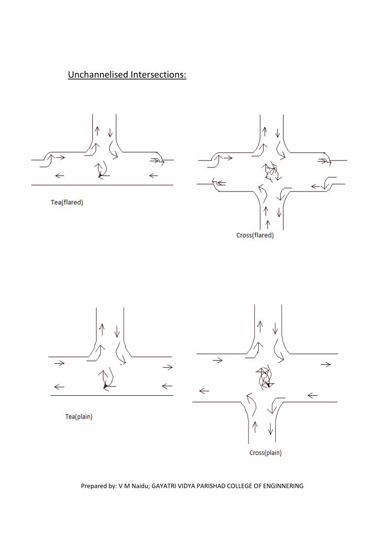
Prepared by: V M Naidu; GAYATRI VIDYA PARISHAD COLLEGE OF ENGINNERING
Unchannelised Intersections:
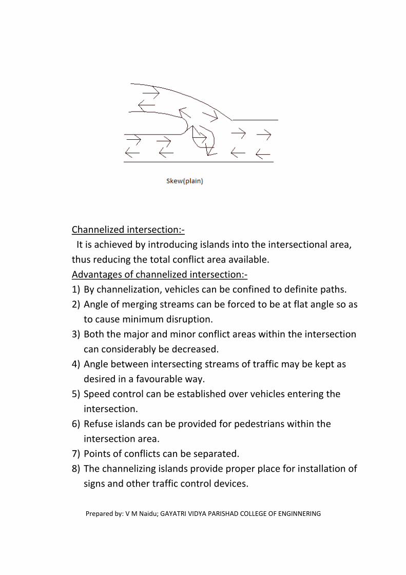
Prepared by: V M Naidu; GAYATRI VIDYA PARISHAD COLLEGE OF ENGINNERING
Channelized intersection:-
It is achieved by introducing islands into the intersectional area,
thus reducing the total conflict area available.
Advantages of channelized intersection:-
1) By channelization, vehicles can be confined to definite paths.
2) Angle of merging streams can be forced to be at flat angle so as
to cause minimum disruption.
3) Both the major and minor conflict areas within the intersection
can considerably be decreased.
4) Angle between intersecting streams of traffic may be kept as
desired in a favourable way.
5) Speed control can be established over vehicles entering the
intersection.
6) Refuse islands can be provided for pedestrians within the
intersection area.
7) Points of conflicts can be separated.
8) The channelizing islands provide proper place for installation of
signs and other traffic control devices.
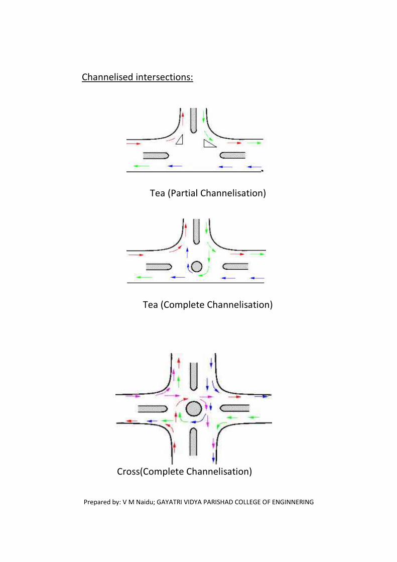
Prepared by: V M Naidu; GAYATRI VIDYA PARISHAD COLLEGE OF ENGINNERING
Channelised intersections:
Tea (Partial Channelisation)
Tea (Complete Channelisation)
Cross(Complete Channelisation)

Prepared by: V M Naidu; GAYATRI VIDYA PARISHAD COLLEGE OF ENGINNERING
Conflicts at intersection:-
Types --> 1)Crossing conflicts
2)Merging conflicts
3)Divergin conflicts

Prepared by: V M Naidu; GAYATRI VIDYA PARISHAD COLLEGE OF ENGINNERING
Conflicts with one-way regulation on one road

Prepared by: V M Naidu; GAYATRI VIDYA PARISHAD COLLEGE OF ENGINNERING
w
Traffic island:-

Prepared by: V M Naidu; GAYATRI VIDYA PARISHAD COLLEGE OF ENGINNERING
These are raised areas constructed within the roadway to
establish physical channelization through which vehicular
traffic may be guided.
The traffic island may be classified based on the function as:
1) Divisional island.
2) Channelizing island.
3) Pedestrian loading islands.
4) Rotary.
Divisional islands:-
Divisional islands are intended to separate opposing flow
of traffic on highway.
By thus dividing the highway into two one-way roadways;
head-on collisions are eliminated and other accidents are
also reduced.
Channelized islands:-
These are used to guide the traffic into proper channel
through the intersection area.
Traffic control devices can be installed on these areas.
The size and shape of the channelizing islands will be very
much depend up the layout and dimensions of the
intersection.
If the islands are not properly designed and placed, there
is a possibility of violation of rules of the traffic resulting in
greater hazards.
Uses of properly designed channelized islands:-

Prepared by: V M Naidu; GAYATRI VIDYA PARISHAD COLLEGE OF ENGINNERING
The area of possible conflicts between traffic stream is
reduced.
They establish the desired angles of crossing and merging
of traffic streams.
They are useful when the direction of floe is to be
changed.
There serve as convenient locations for other traffic
control devices.
They serve as refuge island for pedestrians.
Pedestrian loading islands:-
There are provided at regular bus stops and similar places
for the protection of passengers.
Rotary island:-
It is the large control island of the rotary intersection.
This island is much larger than the central island of
channelized intersection.

Prepared by: V M Naidu; GAYATRI VIDYA PARISHAD COLLEGE OF ENGINNERING
ROTARY INTERSECTION:-
Definition:- It is specialised form of at grade intersection laid out for movement
of traffic in one direction round a central island.
TYPES OF ROTARY INTERSECTIONS:-

Prepared by: V M Naidu; GAYATRI VIDYA PARISHAD COLLEGE OF ENGINNERING
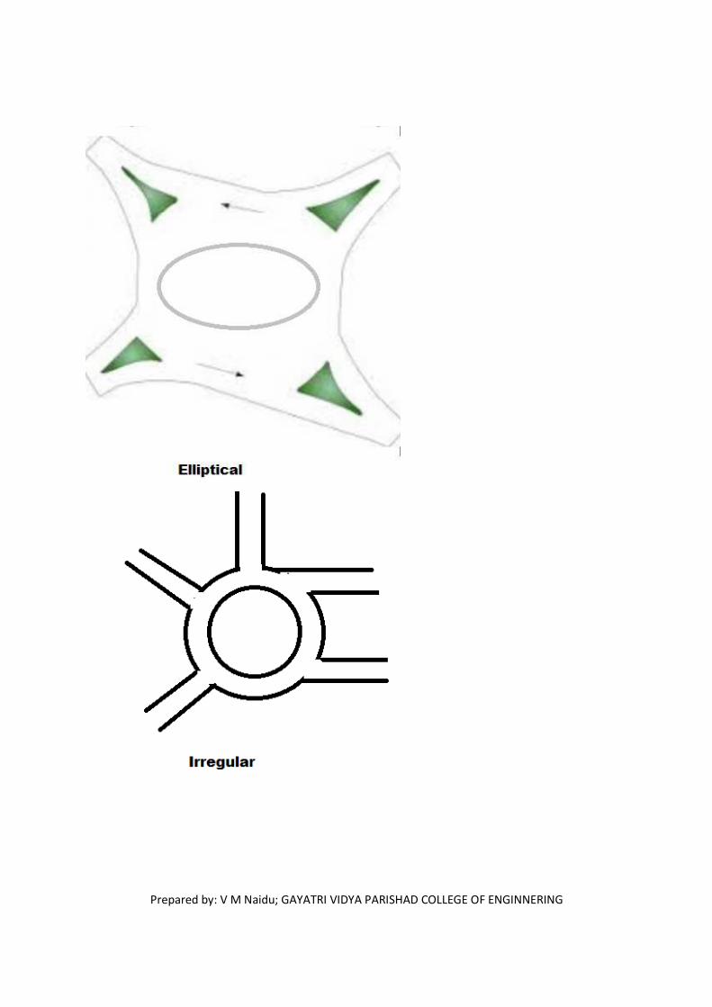
Prepared by: V M Naidu
Prepared by: V M Naidu; GAYATRI VIDYA PARISHAD COLLEGE OF ENGINNERING
OF ENGINNERING
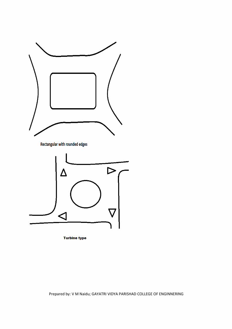
Prepared by: V M Naidu
Prepared by: V M Naidu; GAYATRI VIDYA PARISHAD COLLEGE OF ENGINNERING
OF ENGINNERING

Prepared by: V M Naidu; GAYATRI VIDYA PARISHAD COLLEGE OF ENGINNERING
ROTARY DESIGN ELEMENTS:-
e1 : width at entry
e2 : width of non-weaving section
Diverging: The dividing of a single stream of traffic into separate streams
Merging: The converging of separate streams of traffic into single streams
Weaving: The combined movement of merging and diverging of traffic streams
moving in the same direction
Weaving length: The length of the section of the rotary in which weaving occurs.
DESIGN SPEED:-
� The design speed of a rotary governs various elements such as radii and
weaving lengths.
Rural areas 40Kmph
Urban areas 30Kmph
RADIUS AT ENTRY:-

Prepared by: V M Naidu; GAYATRI VIDYA PARISHAD COLLEGE OF ENGINNERING
� It is the determined by the speed, superelevation and coefficient and
coefficient of friction.
Rural areas 20-35m
Urban areas 15-20m
RADIUS AT EXIST:-
Rexit = 1.5 to 2 times Rentry
� This will (Higher radius) enable the rotary to be cleared rapidly.
RADIUS OF CENTRAL ISLAND:-
Rcentral island = 1.33*Rentry.
� Radius of Central Island may be kept slightly larger than that of curve at
entry, this is to give a slight preference to the traffic already in the rotary.
WEAVING LENGTH:-
� The weaving length determines the ease with which the traffic can merge
and diverge.
� The weaving is decided on the basis of factors such as width of wearing
section, average width of the entry, total traffic and proportion of
weaving traffic in it.
Design
speed(Kmph)
Minimum weaving
length(m)
40 45
30 30
WIDTH OF CARRIAGE WAY AT ENTRY AND EXIT:-
Carriageway width of
approach road
Radius at entry Width of carriage at
entry and exit(m)
7m
6.5
10.5m 7.0

Prepared by: V M Naidu; GAYATRI VIDYA PARISHAD COLLEGE OF ENGINNERING
14m 25-35m 8.0
21m 13.0
7m
15-25m
7.0
10.5m 7.5
14m 10.0
21m 15.0
WIDTH OF ROTARY CARRIAGEWAY:-
W = ((e1+e2)/2)+3.5
ENTRY AND EXIT ANGLES:-
θ entry > θexit
θentry ≈ 60Ө
UNIT-VIII –GRADE SEPERATED INTERSECTION DESIGN
TYPES:-

Prepared by: V M Naidu
Prepared by: V M Naidu; GAYATRI VIDYA PARISHAD COLLEGE OF ENGINNERINGOF ENGINNERING

Prepared by: V M Naidu
Prepared by: V M Naidu; GAYATRI VIDYA PARISHAD COLLEGE OF ENGINNERINGOF ENGINNERING

Prepared by: V M Naidu
Prepared by: V M Naidu; GAYATRI VIDYA PARISHAD COLLEGE OF ENGINNERING
OF ENGINNERING

Prepared by: V M Naidu; GAYATRI VIDYA PARISHAD COLLEGE OF ENGINNERING
AVANTAGES OF GRADE SUPERATION:-
i. Maximum facility is given to the crossing traffic.
ii. There is increased safety for turning safety for turning traffic.
iii. There is overall in comfort and convenience to motorists and saving
in travel time and vehicle operating cost.
iv. The capacity of grade operated intersection can practically that of
two cross roads.
v. Grade separated is an essential part of controlled access highway like
expressing.
vi. It is possible to adopt grade separation for all likely angles and
layout.
vii. Stage construction of additional ramps is possible.
DISADVANTAGES OF GRADE SEPERATION:-
i. It is very costly.
ii. In urban/built up areas, grade separation is difficult.
iii. In flat (or) plain terrain, grade separation may introduce undesirable
crests and sags in the vertical alignment.
ADVANTAGES OF OVERPASS:-
� When the wider road is taken above, the cost of the bridge structure
will be less.
DISADVANTAGES OF OVERPASS:-
� There will be restrictions to sight distance useless long vertical are
provided.
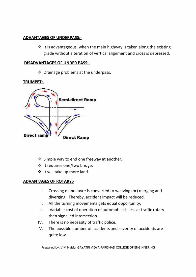
Prepared by: V M Naidu; GAYATRI VIDYA PARISHAD COLLEGE OF ENGINNERING
ADVANTAGES OF UNDERPASS:-
� It is advantageous, when the main highway is taken along the existing
grade without alteration of vertical alignment and cross is depressed.
DISADVANTAGES OF UNDER PASS:-
� Drainage problems at the underpass.
TRUMPET:-
� Simple way to end one freeway at another.
� It requires one/two bridge.
� It will take up more land.
ADVANTAGES OF ROTARY:-
I. Crossing manoeuvre is converted to weaving (or) merging and
diverging . Thereby, accident impact will be reduced.
II. All the turning movements gets equal opportunity.
III. Variable cost of operation of automobile is less at traffic rotary
then signalled intersection.
IV. There is no necessity of traffic police.
V. The possible number of accidents and severity of accidents are
quite low.

Prepared by: V M Naidu; GAYATRI VIDYA PARISHAD COLLEGE OF ENGINNERING
VI. Rotaries are advantages, when the intersecting roads is etween four
and seven.
VII. Capacity of intersections is the highest of all other intersections.
LIMITATIONS OF ROTARY:-
I. Rotary requires comparatively a large area.
II. When there is no. of pedestrian traffic exist, traffic police control is
necessary.
III. When pedestrian and cyclist is more, the design of rotary is
complex.
IV. Where the angle of intersection of two roads is too acute (or) when
there are more than seven roads intersecting, rotaries are
unsuitable.
V. When the distance between intersections are less, rotaries become
troublesome.
VI. When the traffic volume is very low in most of the rural areas in
India, Rotary construction cannot be justified.
IRC Method of signal design:-
Step(i):-
The pedestrian green time required for major and minor roads are
calculated based on walking for major and minor roads are calculated based on
walking speed of 1.2m/s and initial walking of 7.0sec.
Step(ii):-
The green time required for the vehicular traffic on the major road is
increased in proportion to the traffic on the approach roads.
Step(iii):-
The cycle is calculated after allowing amber time of 2.0sec each.
Step(iv):-

Prepared by: V M Naidu; GAYATRI VIDYA PARISHAD COLLEGE OF ENGINNERING
The minimum green time required for clearing vehicles arriving during a
cycle is determined for each of approach assuming that the first vehicle will take
6.0secs. and the subsequent vehicles(PCV) of the queue will be cleared at a rate
of 2.0sec.
Step(v):-
The optimum single cycle time is calculated using webster’s formula. The
saturation flow values may be as 1850, 1890, 1950, 2250, 2550, 2990, PCU/hr
approach road widths 3.0, 3.5, 4.0, 4.5, 5.0,5.5m
For width above 5.5m, the saturation flow may be assumed as 525PCV/hr/mt.
The lost time is calculated from the amber time, intergreen time and initial delay
of 4.0Sec
Step(vi):-
The single cycle time and phases may be revised keeping n view the green
keeping in view the green time required for cleaning the vehicles.
Problem:
At a right angled intersection of two roads, road1 has 4 lanes with a total
width of 12.0m and road2 has two lanes with a total width of 6.6m.The volume of
traffic approaching. The intersection during design hour are 900 and 743PCU/hr
on the two approaches of road 1 and 278 and 180PCU/hr on the two approaches
of road2. Design the signal timing as per IRC guidelines.
Sol:
Design traffic on road1 = higher of the two approach volume per lane
=900/2 =45PCU/hr
Design traffic on road 2 =278PCU/hr
(i) Pedestrian green time road1
Pedestrian green time for road 2 =(6.6/1.2)+7.0 = 12.5sec.

Prepared by: V M Naidu; GAYATRI VIDYA PARISHAD COLLEGE OF ENGINNERING
Green time for road2, G2 = 17.0sec.
(ii) Green time for road1, G1 = 17*(450/278) = 27.5sec
(iii) Adding 2.0sec each towards clearance amber and 2.0sec inter-green
period for each phase, total cycle time required = (2+17+2)+(2+27.5+2) =
52.5sec.
Signal cycle time may be conveniently set in multiplies of fire Secs and
so the cycle time = 55sec.
The extra 2.5sec per cycle may be apportioned to green times of road1
and 2, as 1.5 and 1.0sec and so G1 =27.5+1.5 =29.0sec and G2=17.0 +1.0
= 18sec
(iv) Vehicle arrives per lane cycle on road1
450/55 = 8.2PCU
Minimum green time clearing vehicle on road1 = 6+(8.2-1.0)2= 20.4sec.
Vehicle arrives per cycle on road2 = 6+(5.1-1.0)2 = 14.2sec.
(v) Lost time per cycle =[amber time +inter-green + time lost for initial dealy
of first vehicle] for 2 phases
=(2+2+4)*2 =168
Saturation flow for road1 = 525*6 =3150per/hr
Saturation flow for road2 = 1850+((40*3)/5) =1874per/hr
y1 = 900/3150 = 0.286 y2 = 278/1874 = 0.148
y = 0.286 = 0.148 = 0.434
Optimum cycle time
Co = (1.5L+5)/1-Y = 1.5*16+5/(1-0.434) = 51.2sec
Therefore the cycle time of 55sec designed earlier is acceptable.
Road Green Amber Red Cycle
Road1 29 2 22+2 55
Road2 18 2 33+2 55


