478
Never stop thinking. User’s Manual, V 1.2, Jan. 2001 TriLib A DSP Library for TriCore TM IP Cores

N e v e r s t o p t h i n k i n g .
User ’s Manual , V 1.2, Jan. 2001
TriLibA DSP Library for Tr iCoreTM
IP Cores

Edition 2000-01
Published by Infineon Technologies AG,St.-Martin-Strasse 53,D-81541 München, Germany
© Infineon Technologies AG 2002.All Rights Reserved.
Attention please!
The information herein is given to describe certain components and shall not be considered as warranted characteristics.Terms of delivery and rights to technical change reserved.We hereby disclaim any and all warranties, including but not limited to warranties of non-infringement, regarding circuits, descriptions and charts stated herein.Infineon Technologies is an approved CECC manufacturer.
Information
For further information on technology, delivery terms and conditions and prices please contact your nearest Infineon Technologies Office in Germany or our Infineon Technologies Representatives worldwide (see address list).
Warnings
Due to technical requirements components may contain dangerous substances. For information on the types in question please contact your nearest Infineon Technologies Office.Infineon Technologies Components may only be used in life-support devices or systems with the express written approval of Infineon Technologies, if a failure of such components can reasonably be expected to cause the failure of that life-support device or system, or to affect the safety or effectiveness of that device or system. Life support devices or systems are intended to be implanted in the human body, or to support and/or maintain and sustain and/or protect human life. If they fail, it is reasonable to assume that the health of the user or other persons may be endangered.

User ’s Manual , V 1.1, Sept. 2000
N e v e r s t o p t h i n k i n g .
Tr iL ibA DSP Library for Tr iCore TM

TriLib Revision History: 2000-01 V 1.2
Previous Version: - V 1.1
Page Subjects (major changes since last revision)
New functions (Mathematical, Statistical, FFT)
Current Version - V 1.2
All the functions are ported to GNU Compiler
New functions (Random number, Mixed Adaptive, Mixed FFT, Multirate FIR)
Page 407 Applications
GUI on the host side to provide the visual control for two embedded target applications
Page 425 FAQs
Page 435 Appendix
Page 459 Glossary
We Listen to Your CommentsAny information within this document that you feel is wrong, unclear or missing at all?Your feedback will help us to continuously improve the quality of this document.Please send your proposal (including a reference to this document) to:[email protected]

"Microcontrollers" Templatefor Technical Documentation
1 Introduction . . . . . . . . . . . . . . . . . . . . . . . . . . . . . . . . . . . . . . . . . . . . . . . 151.1 Introduction to TriLib, a DSP Library for TriCore . . . . . . . . . . . . . . . . . . . . 151.2 Features . . . . . . . . . . . . . . . . . . . . . . . . . . . . . . . . . . . . . . . . . . . . . . . . . . . 151.3 Future of the TriLib . . . . . . . . . . . . . . . . . . . . . . . . . . . . . . . . . . . . . . . . . . 161.4 Support Information . . . . . . . . . . . . . . . . . . . . . . . . . . . . . . . . . . . . . . . . . . 16
2 Installation and Build . . . . . . . . . . . . . . . . . . . . . . . . . . . . . . . . . . . . . . . 172.1 TriLib Content . . . . . . . . . . . . . . . . . . . . . . . . . . . . . . . . . . . . . . . . . . . . . . 172.2 Installing TriLib . . . . . . . . . . . . . . . . . . . . . . . . . . . . . . . . . . . . . . . . . . . . . . 182.3 Building TriLib . . . . . . . . . . . . . . . . . . . . . . . . . . . . . . . . . . . . . . . . . . . . . . 182.4 Source Files List . . . . . . . . . . . . . . . . . . . . . . . . . . . . . . . . . . . . . . . . . . . . 19
3 DSP Library Notations . . . . . . . . . . . . . . . . . . . . . . . . . . . . . . . . . . . . . . . 233.1 TriLib Data Types . . . . . . . . . . . . . . . . . . . . . . . . . . . . . . . . . . . . . . . . . . . 233.2 Calling a DSP Library Function from C Code . . . . . . . . . . . . . . . . . . . . . . 233.3 Calling a DSP Library Function from Assembly Code . . . . . . . . . . . . . . . . 233.4 TriLib Example Implementation . . . . . . . . . . . . . . . . . . . . . . . . . . . . . . . . . 233.5 TriLib Implementation - A Technical Note . . . . . . . . . . . . . . . . . . . . . . . . . 24
4 Function Descriptions . . . . . . . . . . . . . . . . . . . . . . . . . . . . . . . . . . . . . . . 294.1 Conventions . . . . . . . . . . . . . . . . . . . . . . . . . . . . . . . . . . . . . . . . . . . . . . . . 294.2 Complex Arithmetic Functions . . . . . . . . . . . . . . . . . . . . . . . . . . . . . . . . . . 31
Addition . . . . . . . . . . . . . . . . . . . . . . . . . . . . . . . . . . . . . . . . . . . . . . . 32Subtraction . . . . . . . . . . . . . . . . . . . . . . . . . . . . . . . . . . . . . . . . . . . . . 32Multiplication . . . . . . . . . . . . . . . . . . . . . . . . . . . . . . . . . . . . . . . . . . . 32Conjugate . . . . . . . . . . . . . . . . . . . . . . . . . . . . . . . . . . . . . . . . . . . . . 33Magnitude . . . . . . . . . . . . . . . . . . . . . . . . . . . . . . . . . . . . . . . . . . . . . 33Phase . . . . . . . . . . . . . . . . . . . . . . . . . . . . . . . . . . . . . . . . . . . . . . . . . 33Shift . . . . . . . . . . . . . . . . . . . . . . . . . . . . . . . . . . . . . . . . . . . . . . . . . . 33
4.3 Vector Arithmetic Functions . . . . . . . . . . . . . . . . . . . . . . . . . . . . . . . . . . . . 854.4 FIR Filters . . . . . . . . . . . . . . . . . . . . . . . . . . . . . . . . . . . . . . . . . . . . . . . . 1064.5 IIR Filters . . . . . . . . . . . . . . . . . . . . . . . . . . . . . . . . . . . . . . . . . . . . . . . . . 1734.6 Adaptive Digital Filters . . . . . . . . . . . . . . . . . . . . . . . . . . . . . . . . . . . . . . . 1974.7 Fast Fourier Transforms . . . . . . . . . . . . . . . . . . . . . . . . . . . . . . . . . . . . . 2414.8 TriCore Implementation Note . . . . . . . . . . . . . . . . . . . . . . . . . . . . . . . . . . 248
First Stage . . . . . . . . . . . . . . . . . . . . . . . . . . . . . . . . . . . . . . . . . . . . 250Butterfly Loop . . . . . . . . . . . . . . . . . . . . . . . . . . . . . . . . . . . . . . . . . . 251Method adapted in the TriLib FFT implementation . . . . . . . . . . . . . 254Group Loop . . . . . . . . . . . . . . . . . . . . . . . . . . . . . . . . . . . . . . . . . . . 254Stage Loop . . . . . . . . . . . . . . . . . . . . . . . . . . . . . . . . . . . . . . . . . . . 254Post Processing . . . . . . . . . . . . . . . . . . . . . . . . . . . . . . . . . . . . . . . . 254Important Note: . . . . . . . . . . . . . . . . . . . . . . . . . . . . . . . . . . . . . . . . 259
4.9 Discrete Cosine Transform (DCT) . . . . . . . . . . . . . . . . . . . . . . . . . . . . . . 3094.10 Inverse Discrete Cosine Transform (IDCT) . . . . . . . . . . . . . . . . . . . . . . . 314
User’s Manual 5 V 1.1, 2000-01

"Microcontrollers" Templatefor Technical Documentation
4.11 Multidimensional DCT (General Information) . . . . . . . . . . . . . . . . . . . . . 3154.12 Mathematical Functions . . . . . . . . . . . . . . . . . . . . . . . . . . . . . . . . . . . . . . 3294.13 Matrix Operations . . . . . . . . . . . . . . . . . . . . . . . . . . . . . . . . . . . . . . . . . . 3634.14 Statistical Functions . . . . . . . . . . . . . . . . . . . . . . . . . . . . . . . . . . . . . . . . . 379
5 Applications . . . . . . . . . . . . . . . . . . . . . . . . . . . . . . . . . . . . . . . . . . . . . . 4015.1 Spectrum Analyzer . . . . . . . . . . . . . . . . . . . . . . . . . . . . . . . . . . . . . . . . . 401
A simple example showing functioning of Spectrum Analyzer. . . . . 4015.2 Sweep Oscillator . . . . . . . . . . . . . . . . . . . . . . . . . . . . . . . . . . . . . . . . . . . 4045.3 Equalizer . . . . . . . . . . . . . . . . . . . . . . . . . . . . . . . . . . . . . . . . . . . . . . . . . 4065.4 Hardware Setup for Applications . . . . . . . . . . . . . . . . . . . . . . . . . . . . . . . 408
6 References . . . . . . . . . . . . . . . . . . . . . . . . . . . . . . . . . . . . . . . . . . . . . . . 417
7 Frequently Asked Questions . . . . . . . . . . . . . . . . . . . . . . . . . . . . . . . . 4197.1 FIR Basics . . . . . . . . . . . . . . . . . . . . . . . . . . . . . . . . . . . . . . . . . . . . . . . . 419
Linear Phase . . . . . . . . . . . . . . . . . . . . . . . . . . . . . . . . . . . . . . . . . . 420Frequency Response . . . . . . . . . . . . . . . . . . . . . . . . . . . . . . . . . . . . 421Numeric Properties . . . . . . . . . . . . . . . . . . . . . . . . . . . . . . . . . . . . . 422
7.2 IIR Basics . . . . . . . . . . . . . . . . . . . . . . . . . . . . . . . . . . . . . . . . . . . . . . . . . 4247.3 FFT . . . . . . . . . . . . . . . . . . . . . . . . . . . . . . . . . . . . . . . . . . . . . . . . . . . . . 425
8 Appendix . . . . . . . . . . . . . . . . . . . . . . . . . . . . . . . . . . . . . . . . . . . . . . . . 4298.1 Introduction . . . . . . . . . . . . . . . . . . . . . . . . . . . . . . . . . . . . . . . . . . . . . . . 4298.2 File Organization . . . . . . . . . . . . . . . . . . . . . . . . . . . . . . . . . . . . . . . . . . . 4308.3 Coding Rules and Conventions for ’C’ and ’C++’ . . . . . . . . . . . . . . . . . . . 4338.4 Coding Rules and Conventions for Assembly Language . . . . . . . . . . . . 4368.5 Testing . . . . . . . . . . . . . . . . . . . . . . . . . . . . . . . . . . . . . . . . . . . . . . . . . . . 4448.6 Compiler Support . . . . . . . . . . . . . . . . . . . . . . . . . . . . . . . . . . . . . . . . . . . 445
9 Glossary . . . . . . . . . . . . . . . . . . . . . . . . . . . . . . . . . . . . . . . . . . . . . . . . 453
User’s Manual 6 V 1.1, 2000-01

"Microcontrollers" Templatefor Technical Documentation
Table 2-1 Directory Structure . . . . . . . . . . . . . . . . . . . . . . . . . . . . . . . . . . . . . . . . 17Table 2-2 Source files . . . . . . . . . . . . . . . . . . . . . . . . . . . . . . . . . . . . . . . . . . . . . 19Table 3-1 TriLib Data Types. . . . . . . . . . . . . . . . . . . . . . . . . . . . . . . . . . . . . . . . . 23Table 3-2 FIR Filter Implementations. . . . . . . . . . . . . . . . . . . . . . . . . . . . . . . . . . 25Table 3-3 Compiler Selection. . . . . . . . . . . . . . . . . . . . . . . . . . . . . . . . . . . . . . . . 26Table 3-4 Tasking Special Data Types . . . . . . . . . . . . . . . . . . . . . . . . . . . . . . . . 26Table 3-5 GHS Special Data Types . . . . . . . . . . . . . . . . . . . . . . . . . . . . . . . . . . . 27Table 3-6 Data Types. . . . . . . . . . . . . . . . . . . . . . . . . . . . . . . . . . . . . . . . . . . . . . 27Table 3-7 DSPEXT CCD Assignments . . . . . . . . . . . . . . . . . . . . . . . . . . . . . . . . 27Table 4-1 Argument Conventions . . . . . . . . . . . . . . . . . . . . . . . . . . . . . . . . . . . . 29Table 4-2 Register Naming Conventions . . . . . . . . . . . . . . . . . . . . . . . . . . . . . . . 30Table 4-3 Complex Data Structure. . . . . . . . . . . . . . . . . . . . . . . . . . . . . . . . . . . . 35Table 8-1 Directory Structure . . . . . . . . . . . . . . . . . . . . . . . . . . . . . . . . . . . . . . . 430Table 8-2 Equal Directives . . . . . . . . . . . . . . . . . . . . . . . . . . . . . . . . . . . . . . . . . 445Table 8-3 Directives with the same functionality but different syntax. . . . . . . . . 446Table 8-4 Datatypes with DSPEXT . . . . . . . . . . . . . . . . . . . . . . . . . . . . . . . . . . 446Table 8-5 Datatypes without DSPEXT . . . . . . . . . . . . . . . . . . . . . . . . . . . . . . . . 447
User’s Manual 7 V 1.1, 2000-01

"Microcontrollers" Templatefor Technical Documentation
User’s Manual 8 V 1.1, 2000-01

Preface
This is the User Manual for TriLib-a DSP library for TriCore. TriCore is the first single-core 32-bit microcontroller-DSP architecture optimized for real-time embedded systems.The DSP core of TriCore is a fixed point one.
This manual describes the implementation of essential algorithms for general digitalsignal processing applications on the TriCore DSP. Characteristics of TriLib and theInstallation and Build procedure are also described.
The source codes are C as well as C++ -callable and thus this library can be used as alibrary of basic functions for developing bigger applications on TriCore. The libraryserves as a user guide for TriCore programmers. It demonstrates how the processor’sarchitecture can be exploited for achieving high performance. There are number of waysto implement an algorithm. The algorithms have been implemented with the primary aimof optimizing execution speed, i.e., minimize number of execution cycles.
The various functions and algorithms implemented and described about in the usermanual are:
• Complex Arithmetic Functions• Vector Arithmetic Functions• Filters– FIR– IIR– Adaptive FIR• Transforms– FFT– DCT• Mathematical Functions• Matrix Operations• Statistical Functions
The user manual describes each function in detail under the following heads:
Signature:
This gives the function interface.
Inputs:
Lists the inputs to the function.
User’s Manual -9 V 1.2, 2000-01

Outputs:
Lists the output of the function.
Return:
Gives the return value of the function if any.
Description:
Gives a brief note on the implementation, the size of the inputs and the outputs,alignment requirements etc.
Pseudocode:
The implementation is expressed as a pseudocode using C conventions.
Techniques:
The techniques employed for optimization are listed here.
Assumptions:
Lists the assumptions made for an optimal implementation such as constraint on buffersize. The input output formats are also given here.
Memory Note:
A detailed sketch showing how the arrays are stored in memory, the nature of the buffers(linear/circular), the alignment requirements of the different buffers, the nature of thearithmetic performed on them (packed, simple). The diagrams give a great insight intothe actual implementation.
Implementation Note:
Gives a very detailed note on the implementation. The codes in TriLib are optimized forspeed. An optimized code is not very easy to understand. The implementation note isvery helpful in overcoming this hurdle. For example, how techniques such as loopunrolling (if employed) help in optimization is described in detail.
Further, the path of an Example calling program, the Cycle Count and Code Size aregiven for each function.
User’s Manual -10 V 1.2, 2000-01

Organization
Chapter 1, Introduction, gives a brief introduction of the TriLib and its features.
Chapter 2, Installation and Build, describes the TriLib content, how to install and buildthe TriLib.
Chapter 3, DSP Library Notations, describes the DSP Library data types, arguments,calling a function from the C code and the assembly code, and the implementation notes.
Chapter 4, Function Descriptions, describes the Complex arithmetic functions, Vectorarithmetic functions, FIR filters, IIR filters, Adaptive filters, Fast Fourier Transforms,Discrete Cosine Transform, Mathematical functions, Matrix operations and Statisticalfunctions. Each function is described with its signature, inputs, outputs, return, briefdescription, pseudocode, techniques used, assumptions made, memory note,implementation details, example, cycle count and code size.
Chapter 5, Applications, describes the applications such as Spectrum Analyzer, SweepOscillator and Equalizer using implemented TriLib functions.
Chapter 6, References, gives the list of related references.
Chapter 7, FAQs, gives Frequently Asked Questions about FIR, IIR and FFT.
Chapter 8, Appendix, gives the conventions for C and assembly code, file namingconventions, directory structure and porting for the Tasking, GHS and GNU compilers.
Chapter 9, Glossary, gives a brief explanation of the terminology used in the TriLib usermanual in alphabetical order.
What’s new?
• New functions have been added• All functions are now supported on GNU compiler also• Three Applications showing the use of functions from TriLib are added
User’s Manual -11 V 1.2, 2000-01

• A powerful GUI on the host side is added to provide visual control to the embeddedtarget application
• FAQs, Appendix and Glossary are added• The GHS and Tasking compiler now have an extra implementation for C and C++
respectively thereby to give flexibility to the user to use anyone for their convenience• TriLib Classes for the much bigger TriApp foundation classes called as TFC (TriCore
application foundation classes) to enable developers to scale up their signalprocessing applications
Acknowledgements
The technical substance of this manual has been mainly developed by the Infineon’sTriLib development team. These are designed, developed and tested over the hardware.We in advance would like to acknowledge users for their feedback and suggestions toimprove this product. The development team would like to thank Dieter Stengl, Directorfor CMD TO S/W for all his support and encouragement. Rakesh Verma, TechnicalManager, Wipro, for his support to the Wipro’s development team and co-ordination withthe Infineon team. Thomas Varghese, Arun Naik, Sreenivas, Mahesh for their valuablecontribution in giving the feedback on user manual and active participation in some ofthe code reviews and also for their technical support. The team also recognizes the effortof Savitha for her patience in meticulously preparing, typesetting and reviewing the UserManual. We also would like to thank our marketing team for their comments and inputs.
Mark Nuchimowicz, Ramachandra, Rashmi, Preethi, Manoj, Ankur and Nagaraj
TriLib Development team - Infineon
Acronyms and Definitions
Acronyms and Definitions
Acronyms Definitions
DCT Discrete Cosine Transform
DFT Discrete Fourier Transform
DIF Decimation-In-Frequency
DIT Decimation-In-Time
DLMS Delayed Least Mean Square
DSP Digital Signal Processing
User’s Manual -12 V 1.2, 2000-01

Documentation/Symbol Conventions
The following is the list of documentation/symbol conventions used in this manual.
TriLib DSP Library functions for TriCore
FFT Fast Fourier Transform
FIR Finite Impulse Response
IIR Infinite Impulse Response
Documentation/Symbol Conventions
Documentation/Symbol convention
Description
Courier Pseudocode
( * ) Denotes Q format multiplication
Times-italic File name
Pointer
Circular pointer
Acronyms and Definitions
Acronyms Definitions
User’s Manual -13 V 1.2, 2000-01

User’s Manual -14 V 1.2, 2000-01

Introduction
1 Introduction
1.1 Introduction to TriLib, a DSP Library for TriCore
The TriLib, a DSP Library for TriCore is C-callable, hand-coded assembly, generalpurpose signal processing routines. These routines are extensively used in real-timeapplications where speed is critical.
The TriLib includes more than 60 commonly used DSP routines. The throughput of thesystem using the TriLib routines is considerably better than those achieved using theequivalent code written in ANSI C language. The TriLib significantly helps inunderstanding the general purpose signal processing routines, its implementation onTriCore. It also reduces the DSP application development time. The TriLib also providesthe source code. Few applications are also provided as part of TriLib to demonstrate theusage of functions.
The routines are broadly classified into the following functional categories:
• Complex Arithmetic• Vector Arithmetic• FIR Filters• IIR Filters• Adaptive Filters• Fast Fourier Transforms• Discrete Cosine Transform• Mathematical functions• Matrix operations• Statistical functions
1.2 Features
• Covers the common DSP algorithms with Source codes• Hand-coded and optimized assembly modules• C/C++ callable functions on Tasking, GreenHills and GNU compilers• Multi platform support - Win 95, Win 98, Win NT• Bit-exact reference C codes for easy understanding and verification of the algorithms• Assembly implementation tested for bit exactness against model C codes• Workarounds implemented to take care of known Core errors• Examples to demonstrate the usage of functions• Example input test vectors and the output test data for verification
User’s Manual 1-15 V 1.2, 2000-01

Introduction
• Comprehensive Users manual covering many aspects of implementation• Useful Applications built using the TriLib to demonstrate the product• Powerful User friendly GUI interface for applications built using TriLib• TriApp-TriLib application foundation class for extending the TriLib functionality• Supports the Object Oriented application development in C++ and Java• User helpful Demoshield based setup and registration program
1.3 Future of the TriLib
The planned future releases will have the following improvements.
• Expansion of the library by adding more number of functions in the domains such asimage processing, speech processing and the generic core routines of DSP.
• Upgrading the existing 16 bit functions to 32 bit
1.4 Support Information
Any suggestions for improvement, bug report if any, can be sent via e-mail to
Visit www.infineon.com for update on TriLib releases.
User’s Manual 1-16 V 1.2, 2000-01

Installation and Build
2 Installation and Build
2.1 TriLib Content
The following table depicts the TriLib content with its directory structure.
Table 2-1 Directory Structure
Directory name
Contents Files
TriLib Directories which has all the files related to the TriLib
None
source Directories Tasking, GreenHills and GNU
None
Tasking Individual directories for each functional category. Each directory has respective assembly language implementation files of the library functions
*.asm
GreenHills Individual directories for each functional category. Each directory has respective assembly language implementation files of the library functions
*.tri
GNU Individual directories for each functional category. Each directory has respective assembly language implementation files of the library functions
*.S
include Directories Tasking, GreenHills and GNU and common include file for ’C’ of all the three compilers
TriLib.h
Tasking Include files for assembly routine *.inc for assembly
GreenHills Include files for assembly routine *.h for assembly
GNU Include files for assembly routine *.h for assembly
docs User ManualConvention Manualreadme.txt
*.fm, *.pdf*.doc*.txt
examples Directories Tasking and GreenHills None
User’s Manual 2-17 V 1.2, 2000-01

Installation and Build
2.2 Installing TriLib
TriLib is distributed as a self extracting ZIP file. To install the TriLib on the system, unzipthe ZIP file and run setup. This will install all the files in the respective directories.
The directory structure is as given in “TriLib Content” on Page 17
2.3 Building TriLib
Include the TriLib.h into your project and also include the same into the files that need tocall the library function like:
#include “TriLib.h”
Set the include path in the tool that you are using for both the project as well as each ofthe files you have included (it is observed that sometimes you get errors if it is not set inthe options of each individual files). Please refer the documentation of the Tasking,GreenHills and GNU for more details.
Tasking Individual directories for each functional category. Each directory has respective example ‘c’ and ’cpp’ functions to depict the usage of TriLib
*.c, *.cpp
GreenHills Individual directories for each functional category. Each directory has respective example ‘cpp’ and ’c’ functions to depict the usage of TriLib
*.cpp, *.c
GNU Individual directories for each functional category. Each directory has respective example ‘c’ functions to depict the usage of TriLib
*.c
refcode Individual directories for each functional category. Each directory has respective reference ‘C’ code of the corresponding assembly implementation in source directory, which works on Tasking compiler
None
build Build information *.pjt, *.bld
testvectors Test vectors for the different functions in their respective directories
*.dat
Table 2-1 Directory Structure
User’s Manual 2-18 V 1.2, 2000-01

Installation and Build
In case of Tasking, the #define part for _TASKING selection box should be checked andin case of GreenHills it should be typed manually as _GHS, otherwise it might give lot ofcompiler errors.
In both the compilers the DSPEXT has to be defined in the project options for both theassembly sources and the c files in the respective project options when the DSPextension for respective compilers (Tasking and GreenHills) have to be used.
For without DSP extension don’t define DSPEXT for c compiler option. For assembleroption set DSPEXT=0. GNU compiler doesn’t support data types for DSP. So DSPEXTneed not be defined or undefined in case of GNU compiler.
If the .cpp file is to be used, in case of Tasking or GreenHills compiler, the macro_cplusplus is to be defined under compiler options.
For setting the other CCD, such as H/W workarounds, use the assembler options.
Now include the respective source files for the required functionality into your project.Refer the functionality table, Table 2-2
Build the system and start using the library.
2.4 Source Files List
Table 2-2 Source files
Tasking GreenHills GNU
Complex Arithmetic functions
CplxOp_16.asmCplxOp_32.asm
CplxOp_16.tri CplxOp_32.tri
CplxOp_16.S CplxPhMag_16.SCplxOp_32.S CplxPhMag_32.S
Vector Arithmetic functions
VectOp_16.asm VectOp_16.tri VectOp1_16.tri
VectOp_16.S VectOp1_16.S
FIR filters
Fir_16.asmFirBlk_16.asmFir_4_16.asmFirBlk_4_16.asm
Fir_16.triFirBlk_16.triFir_4_16.triFirBlk_4_16.tri
Fir_16.SFirBlk_16.SFir_4_16.SFirBlk_4_16.S
User’s Manual 2-19 V 1.2, 2000-01

Installation and Build
FirSym_16.asmFirSymBlk_16.asmFirSym_4_16.asmFirSymBlk_4_16.asmFirDec_16.asmFirInter_16.asm
FirSym_16.triFirSymBlk_16.triFirSym_4_16.triFirSymBlk_4_16.triFirDec_16.triFirInter_16.tri
FirSym_16.SFirSymBlk_16.SFirSym_4_16.SFirSymBlk_4_16.SFirDec_16.SFirInter_16.S
IIR filters
IirBiq_4_16.asmIirBiqBlk_4_16.asmIirBiq_5_16.asmIirBiqBlk_5_16.asm
IirBiq_4_16.triIirBiqBlk_4_16.triIirBiq_5_16.triIirBiqBlk_5_16.tri
IirBiq_4_16.SIirBiqBlk_4_16.SIirBiq_5_16.SIirBiqBlk_5_16.S
Adaptive filters
Dlms_4_16.asmDlmsBlk_4_16.asmCplxDlms_4_16.asmCplxDlmsBlk_4_16.asmDlms_2_16x32.asmDlmsBlk_2_16x32.asm
Dlms_4_16.triDlmsBlk_4_16.triCplxDlms_4_16.triCplxDlmsBlk_4_16.triDlms_2_16x32.triDlmsBlk_2_16x32.tri
Dlms_4_16.SDlmsBlk_4_16.SCplxDlms_4_16.SCplxDlmsBlk_4_16.SDlms_2_16x32.SDlmsBlk_2_16x32.S
FFT
FFT_2_16.asmFFT_2_32.asmFFT_2_16X32.asm
FFT_2_16.triFFT_2_32.triFFT_2_16X32.tri
FFT_2_16.SFFT_2_32.SFFT_2_16X32.S
DCT
DCT_2_8.asm DCT_2_8.tri DCT_2_8.S
Mathematical Functions
Sine_32.asmCos_32.asmArctan_32.asmSqrt_32.asmLn_32.asmAntiLn_16.asmExpn_16.asmXpowY_32.asmRandInit_16.asmRand_16.asm
Sine_32.triCos_32.triArctan_32.triSqrt_32.triLn_32.triAntiLn_16.triExpn_16.triXpowY_32.triRandInit_16.triRand_16.tri
Sine_32.SCos_32.SArctan_32.SSqrt_32.SLn_32.SAntiLn_16.SExpn_16.SXpowY_32.SRandInit_16.SRand_16.S
Matrix Functions
Table 2-2 Source files
User’s Manual 2-20 V 1.2, 2000-01

Installation and Build
MatAdd_16.asmMatSub_16.asmMatMult_16.asmMatTrans_16.asm
MatAdd_16.triMatSub_16.triMatMult_16.triMatTrans_16.tri
MatAdd_16.SMatSub_16.SMatMult_16.SMatTrans_16.S
Statistical Functions
ACorr_16.asmConv_16.asmAvg_16.asm
ACorr_16.triConv_16.triAvg_16.tri
ACorr_16.SConv_16.SAvg_16.S
Table 2-2 Source files
User’s Manual 2-21 V 1.2, 2000-01

Installation and Build
User’s Manual 2-22 V 1.2, 2000-01

DSP Library Notations
3 DSP Library Notations
3.1 TriLib Data Types
The TriLib handles the following fractional data types.
3.2 Calling a DSP Library Function from C Code
After installing the TriLib, do the following to include a TriLib function in the source code.
1. Include the TriLib.h include file 2. Include the source file that contains required DSP function into the project along with
the other source files3. Include TriConv.inc (Tasking) or TriConv.h (GreenHills)4. Set the include paths to point the location of the TriLib.h 5. Set the Compiler Conditional Directives (CCDs) for selection of DSP extension 6. Set the Compiler Conditional Directives (CCDs) to generate code with workarounds
for the H/W bugs7. Build the system
3.3 Calling a DSP Library Function from Assembly Code
The TriLib functions are written to be used from C. Calling the functions from assemblylanguage source code is possible as long as the calling function conforms to the TriCorecalling conventions. Refer TriCore Calling Conventions manual for more details.
3.4 TriLib Example Implementation
The examples of how to use the TriLib functions are implemented and are placed inexamples subdirectory. This subdirectory contains a subdirectory for set of functions.
Table 3-1 TriLib Data Types
1Q15 (DataS) 1Q15 operand is represented by a short data type (frac16/_sfract) that is predefined as DataS in TriLib.h header file.
1Q31 (DataL) 1Q31 operand is represented by a long data type (frac32/_fract) that is predefined as DataL in TriLib.h header file.
CplxS Complex data type contains the two 1Q15 data arranged in Re-Im format.
CplxL Complex data type contains the two 1Q31 data arranged in Re-Im format.
User’s Manual 3-23 V 1.2, 2000-01

DSP Library Notations
3.5 TriLib Implementation - A Technical Note
3.5.1 Memory Issues
The TriLib is implemented with the known alignment constraints for the TriCore memoryaddressing architecture. The following information gives the alignment and sizesconditions in order to work properly.
Halfword alignment for ld.d and st.d is only allowed when the source or destinationaddress is located in on-chip memory. For external memory accesses over TriCore’speripherals bus, doubleword access must be word aligned (TriCore Architecture Manualp.13).
The size and length of a circular buffer have the following restrictions (TriCoreArchitecture Manual p.13).
• The start of the buffer start must be aligned to a 64-bit boundary.• The length of the buffer must be a multiple of the data size, where the data size is
determined from the instruction being used to access the buffer.
Different alignment requirements for ld.d and st.d for internal and external memoriesimpose different alignment of data in functions that use those instructions. In some cases(for example filter delay-buffer defined as circular-buffer) halfword aligned accesses tothe data is required which prohibit the location of such data structures in externalmemory.
For example Fir_4_16() function, the delay-buffer of the filter is defined as circular-buffer.
In this case, when located in internal memory the buffer must have doublewordalignment (circular-buffer). After each call to the function the start position of the delay-buffer is shifted (with circular update) by halfword. The delay-buffer cannot be located inexternal memory because the load from the delay-buffer is executed by ld.d instructionand word alignment is no more satisfied.
3.5.2 Optimization Approach
Extended parallelism of the processor architecture increases the speed of the algorithmsexecution, but at the same time imposes some constraints on the size of Input-Buffers.So for example Fir_4_16() FIR filter executes at maximal possible speed on the TriCorebut the size must be multiple of 4.
In the implementation of the algorithms following optimizations are applied:
• Packed arithmetic
User’s Manual 3-24 V 1.2, 2000-01

DSP Library Notations
• Mixed packed /simple arithmetic• Simple arithmetic
From the point of view of size of the algorithm (Vector length, Filter length) two cases canbe identified:
• Constraint on the dimension of vector, order of filter • Arbitrary size
Best performance can be achieved with some constrains on the size in which case fullypacked arithmetic is used in the kernel loop. Arbitrary size (not for all algorithms) can beachieved by using
• Simple arithmetic in the kernel loop • Mixed packed/simple arithmetic, partitioning of the algorithm size so that the kernel
loop uses packed arithmetic with conditional post processing to achieve arbitrary size
To achieve maximal performance and flexibility some functions have severalimplementations optimized for specific target requirements.
Following implementations can be recognized:
• On sample, optimized for single sample processing• On block, optimized for block processing• Best performance with restriction on size • Arbitrary size, trade-off between performance and flexibility
For example FIR filter is implemented as
The SIMD instructions are exploited in the FFT by the special arrangement of the Realand Imaginary parts of the complex number. The Real:Imag format is the conventionalmethod of storing the complex number x+jy. In this case two complex numbers x0+jy0and x1+jy1 is arranged as x0x1 and j(y0y1).
Table 3-2 FIR Filter Implementations
Fir_16() Sample processing, trade-off on performance, arbitrary size
Fir_4_16() Sample processing, best performance, size restriction
FirBlk_16() Block processing, trade-off on performance, arbitrary size
FirBlk_4_16() Block processing, best performance, size restriction
User’s Manual 3-25 V 1.2, 2000-01

DSP Library Notations
3.5.3 Options in Library Configurations
Set of Conditional Compile Directives (CCD) on the C language level and assembly leveldefine the configuration of the TriLib.
3.5.3.1 Compiler
Compiler selection is based on two CCD
In the current implementation of the TriLib this setting is only evaluated in TriLib.h headerfile which is common to all the compilers.
All the library functions and examples have dedicated implementations for each compilerand are not influenced by this setting.
3.5.3.2 DSP Extensions
To improve the DSP functionality on the C language level Tasking compiler supportsthree additional special DSP specific intrinsic data types to perform fixed point arithmetic.Refer to the tools documentation for details.
To efficiently implement a circular buffer in the C language additional qualifier _circ isdefined by Tasking. This can be used in conjunction with the other data types.
Table 3-3 Compiler Selection
_Tasking CCD on the C level for selecting the Tasking compiler
_GHS CCD on the Cpp level for selecting the GHS compiler
COR1 Hardware workaround for TriCore ver1.2
COR14 Hardware workaround for TriCore ver1.2
CPU5 Hardware workaround for TriCore ver1.3
Table 3-4 Tasking Special Data Types
_sfract 16 bits: 1 sign bit + 15 mantissa bits
_fract 32 bits: 1 sign bit + 31 mantissa bits
_accum 64 bits: 1 sign bit + 17 integral bits + 46 mantissa bits
User’s Manual 3-26 V 1.2, 2000-01

DSP Library Notations
GHS compiler, extended support of DSP functionality is implemented by defining C++classes.
Circular buffer pointer is implemented in GHS C++ compiler as a templatized class.
To make the library portable, TriLib function arguments use following predefined datatypes.
Depending on the compiler used and the setting of _DSPEXT CCD followingassignments are used (implemented in TriLib.h)
DSPEXT CCD has effect on the C/C++ level as well on the assembly implementationsof the TriLib function.
3.5.4 Workarounds of known Behavioral Deviations
The instruction set of TriCore is defined in different syntax for the GreenHills and TaskingTool sets. There are different deviations in each of the compilers. Particularly theGreenHills doesn’t support some instructions in its Multi 2000 ver 2.0 and also there arebehavioral changes in the ver 2.0.2. This can be potential risk in the development for
Table 3-5 GHS Special Data Types
frac16 16 bits: 1 sign bit + 15 mantissa bits
frac32 32 bits: 1 sign bit + 31 mantissa bits
frac64 64 bits: 1 sign bit + 17 integral bits + 46 mantissa bits
Table 3-6 Data Types
DataS 16-bit operands
DataL 32-bit operands
cptrDataS circular-pointer to DataS circular-buffer
cptrDataL circular-pointer to DataL circular-buffer
Table 3-7 DSPEXT CCD Assignments
DSPEXT=FALSE DSPEXT=TRUE
Tasking, GHS, GNU Tasking GHS
DataS short _sfract frac16
DataL int _fract frac32
CptrDataS struct (TriLib.h) _sfract _circ* circptr<frac16>
User’s Manual 3-27 V 1.2, 2000-01

DSP Library Notations
people to migrate from one compiler to other. To give some instances of the knowndeviations.
Conditional move instruction (cmov,cmovn) is not supported in GHS ver 2.0 in this caseselect (sel,seln) instructions has to be used.
The data memory addressing is bit complicated in GHS, there are special syntax to dothe same for instance syntaxes such as %sdaoff etc., are used. Refer the GHSdocumentation for more details.
The jz has problems in GHS ver 2.0 so in order to workaround this, usage of jeq isencouraged, The instruction jz works on GHS ver 2.0.2. The Sine/Cosine functions usejz instruction and will run on ver 2.0.2.
3.5.5 Testing Methodology
The TriLib is tested on GHS, Tasking simulator and TriCore TC10GP TriBoard ver2.4.
The Hardware workarounds have to be enabled only if the TriLib is intended to run onTC10GP (TriCore ver1.2, ver1.3) processor hardware.
User’s Manual 3-28 V 1.2, 2000-01

Function Descriptions
4 Function DescriptionsEach function is described with its signature, inputs, outputs, return, brief description,pseudocode, techniques used, assumptions made, memory note, how it is implemented,example, cycle count and code size.
Functions are classified into the following categories.
• Complex Arithmetic functions• Vector functions• FIR filters• IIR filters• Adaptive filters• Fast Fourier Transforms• Discrete Cosine Transform• Mathematical functions• Matrix operations• Statistical functions
4.1 Conventions
4.1.1 Argument Conventions
The following conventions have been followed while describing the arguments for eachindividual function.
Table 4-1 Argument Conventions
Argument Convention
X,Y Input data or input data vector
R Output data
nX, nY, nR The size of vectors X, Y, and R respectively. In functions
where nX = nY = nR, only nX has been used
H Filter coefficient vector (filter routines only)
nH The size of vector H. Usually not defined explicitly
DataS Data type definition equating a short, a 16-bit value representing a 1Q15 number
DataL Data type definition equating a long, a 32-bit value representing a 1Q31 number
DataD Reserved for 64-bit value
User’s Manual 4-29 V 1.2, 2000-01

Function Descriptions
4.1.2 Register Naming Conventions
The following register naming conventions have been followed.
cptrDataS Circular pointer structure
CplxS Data type definition equating a short, a 16-bit value representing a 1Q15 complex number
CplxL Data type definition equating a long, a 32-bit value representing a 1Q31 complex number
aR Pointer to Output-Buffer
Table 4-2 Register Naming Conventions
Argument Convention
a Address register or data type prefix
ca Circular buffer address register pair
Table 4-1 Argument Conventions
Argument Convention
User’s Manual 4-30 V 1.2, 2000-01

Function Descriptions
4.2 Complex Arithmetic Functions
4.2.1 Complex Numbers
A complex number z is an ordered pair (x,y) of real numbers x and y, written as
z= (x,y)
where x is called the real part and y the imaginary part of z.
4.2.2 Complex Number Representation
A complex number can be represented in different ways, such as
In the complex functions implementation, the rectangular form is considered.
4.2.3 Complex Plane
The geometrical representation of complex numbers as points in the plane is of greatimportance. Choose two perpendicular coordinate axis in the Cartesian coordinatesystem. The horizontal x-axis is called the real axis, and the vertical y-axis is called theimaginary axis. Plot a given complex number z=(x,y) = x + iy as the point P withcoordinates (x, y). The xy-plane in which the complex numbers are represented in thisway is called the Complex Plane. This is also called as the Argand diagram after theFrench mathematician Jean Robert Argand.
Rectangular form : [4.1]
Trigonometric form : [4.2]
Exponential form : [4.3]
Magnitude and angle form : [4.4]
C R iI+=
C M φ( ) j φ( )sin+cos[ ]=
C Meiφ
=
C M φ∠=
User’s Manual 4-31 V 1.2, 2000-01

Function Descriptions
Figure 4-1 The Complex Plane (Argand Diagram)
4.2.4 Complex Arithmetic
Addition
if z1 and z2 are two complex numbers given by z1 =x1+iy1 and z2 = x2 + iy2,
z1+z2 = (x1+iy1) + (x2 + iy2) = (x1+x2) + i(y1+y2) [4.5]
Subtraction
if z1 and z2 are two complex numbers given by z1 =x1+iy1 and z2 = x2 + iy2,
z1-z2 = (x1-x2) + i(y1-y2) [4.6]
Multiplication
if z1 and z2 are two complex numbers given by z1 =x1+iy1 and z2 = x2 + iy2,
z1.z2 = (x1+iy1).(x2 + iy2) = x1x2 + ix1y2 + iy1x2 + i2 y1y2
= (x1x2 - y1y2) + i(x1y2 + x2y1) [4.7]
P
O (Real Axis)
(ImaginaryAxis)
x
y
z = x + iy
User’s Manual 4-32 V 1.2, 2000-01

Function Descriptions
Conjugate
The complex conjugate, z of a complex number z = x+iy is given by
z = x - iy [4.8]
and is obtained by geometrically reflecting the point z in the real axis.
Magnitude
The magnitude of a complex number z=x+iy is given by
[4.9]
Geometrically, |z| is the distance of the point z from the origin.
|z1-z2| is the distance between z1 and z2.
Phase
The phase of complex number z=x+iy is given by
phase = tan-1(y/x) [4.10]
Shift
Shifting of a complex number is indicated by the shift value. Left shifting is done if the shift value is positive and right shifting is done if shift value is negative.
[4.11]
z x2
y2
+=
Zr x abs shiftval( ) if shiftval 0<( ),»=
else x shiftval«( )Zi y abs shiftval( ) if shiftval 0<( ),»=
else y shiftval«( )
User’s Manual 4-33 V 1.2, 2000-01
Function Descriptions
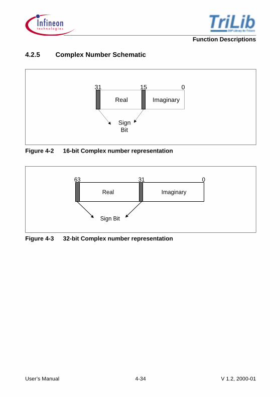
4.2.5 Complex Number Schematic
Figure 4-2 16-bit Complex number representation
Figure 4-3 32-bit Complex number representation
31 15 0
Real Imaginary
SignBit
63 31 0
Real Imaginary
Sign Bit
User’s Manual 4-34 V 1.2, 2000-01

Function Descriptions
4.2.6 Complex Data Structure
4.2.7 Descriptions
The following complex arithmetic functions for 16 bit and 32 bit are described.
• Addition (with and without saturation)• Subtraction (with and without saturation)• Multiplication (with and without saturation)• Conjugate• Magnitude• Phase• Shift
Table 4-3 Complex Data Structure
Tasking GHS ANSI C/GNU
16 bit
typedef struct{ _sfract imag; _sfract real;} CplxS;
typedef struct{ frac16 imag; frac16 real;} CplxS;
typedef struct{ short imag; short real;} CplxS;
32 bits
typedef struct{ _fract imag; _fract real;} CplxL;
typedef struct{ frac32 imag; frac32 real;} CplxL;
typedef struct{ long imag; long real;} CplxL;
User’s Manual 4-35 V 1.2, 2000-01

Function Descriptions
CplxAdd_16 Complex Number Addition for 16 bits
Signature CplxS CplxAdd_16(CplxS X, CplxS Y );
Inputs X : 16 bit Complex input value
Y : 16 bit Complex input value
Output None
Return The sum of two complex numbers as a 16 bit complex number
Description This function computes the sum of two 16 bit complex numbers. Wraps around the result in case of overflow.The algorithm is as follows
[4.12]
Pseudo code
{ R.real = X.real + Y.real; //add the real part R.imag = X.imag + Y.imag; //add the imaginary part return R;}
Techniques None
Assumptions • Input and output has a real and an imaginary part packedas 16 bit data to make a 32 bit complex data
Rr xr yr+=
Ri xi yi+=
User’s Manual 4-36 V 1.2, 2000-01

Function Descriptions
Memory Note
Figure 4-4 Complex Number addition for 16 bits
Example Trilib\Example\Tasking\CplxArith\expCplx.c, expCplx.cpp
Trilib\Example\GreenHills\CplxArith\expCplx.cpp,expCplx.c
Trilib\Example\GNU\CplxArith\expCplx.c
Cycle Count 1+2
Code Size 6 bytes
CplxAdd_16 Complex Number Addition for 16 bits (cont’d)
31 15 0 31 15 0
+
+
31 15 0
Real Imaginary Real Imaginary
Real Imaginary
User’s Manual 4-37 V 1.2, 2000-01

Function Descriptions
CplxAdds_16 Complex Number Addition for 16 bits with saturation
Signature CplxS CplxAdds_16(CplxS X, CplxS Y );
Inputs X : 16 bit Complex input value
Y : 16 bit Complex input value
Output None
Return The sum of two complex numbers as a 16 bit saturated complex number
Description This function computes the sum of two 16 bit complex numbers. In case of overflow, this saturates the result to 0x7FFF for positive values and 0x8000 for negative values. This is applicable for both real and imaginary part of the complex number. The algorithm is as follows
[4.13]
Pseudo code
{ R.real = (frac16 sat)(X.real + Y.real); //add the real part R.imag = (frac16 sat)(X.imag + Y.imag); //add the imaginary part return R;}
Techniques None
Assumptions • Input and output has a real and an imaginary part packedas 16 bit data to make a 32 bit complex data
Rr xr yr+=
Ri xi yi+=
User’s Manual 4-38 V 1.2, 2000-01

Function Descriptions
Memory Note
Figure 4-5 Complex number addition for 16 bits with saturation
Example Trilib\Example\Tasking\CplxArith\expCplx.c, expCplx.cpp
Trilib\Example\GreenHills\CplxArith\expCplx.cpp,expCplx.c
Trilib\Example\GNU\CplxArith\expCplx.c
Cycle Count 1+2
Code Size 6 bytes
CplxAdds_16 Complex Number Addition for 16 bits with saturation (cont’d)
31 15 0 31 15 0
+
+
Real Imaginary Real Imaginary
31 15 0
Real Imaginary
Sat Sat
User’s Manual 4-39 V 1.2, 2000-01

Function Descriptions
CplxSub_16 Complex Number Subtraction for 16 bits
Signature CplxS CplxSub_16(CplxS X, CplxS Y );
Inputs X : 16 bit Complex input value
Y : 16 bit Complex input value
Output None
Return The difference of two complex numbers as a 16 bit complex number
Description This function finds the difference of two 16 bit complex numbers. Wraps around the result in case of underflow. The algorithm is as follows.
[4.14]
Pseudo code
{ R.real = X.real - Y.real; //subtract the real part R.imag = X.imag - Y.imag; //subtract the imaginary part return R;}
Techniques None
Assumptions • Input and output has a real and an imaginary part packedas 16 bit data to make a 32 bit complex data
Rr xr yr–=
Ri xi yi–=
User’s Manual 4-40 V 1.2, 2000-01

Function Descriptions
Memory Note
Figure 4-6 Complex number subtraction for 16 bits
Example Trilib\Example\Tasking\CplxArith\expCplx.c, expCplx.cpp
Trilib\Example\GreenHills\CplxArith\expCplx.cpp,expCplx.c
Trilib\Example\GNU\CplxArith\expCplx.c
Cycle Count 1+2
Code Size 6 bytes
CplxSub_16 Complex Number Subtraction for 16 bits (cont’d)
31 15 0 31 15 0
-
-
31 15 0
Real Imaginary Real Imaginary
Real Imaginary
User’s Manual 4-41 V 1.2, 2000-01

Function Descriptions
CplxSubs_16 Complex Number Subtraction for 16 bits with saturation
Signature CplxS CplxSubs_16(CplxS X, CplxS Y );
Inputs X : 16 bit Complex input value
Y : 16 bit Complex input value
Output None
Return The difference of two complex numbers as a 16 bit saturated complex number
Description This function finds the difference of two 16 bit complex numbers. In case of overflow, this saturates the result to 0x7FFF for positive values and 0x8000 for negative values. The algorithm is as follows.
[4.15]
Pseudo code
{ R.real = (frac16 sat)(X.real - Y.real); //subtract the real part R.imag = (frac16 sat)(X.imag - Y.imag); //subtract the imaginary part return R;}
Techniques None
Assumptions • Input and output has a real and an imaginary part packedas 16 bit data to make a 32 bit complex data
Rr xr yr–=
Ri xi yi–=
User’s Manual 4-42 V 1.2, 2000-01

Function Descriptions
Memory Note
Figure 4-7 Complex number subtraction for 16 bits with saturation
Example Trilib\Example\Tasking\CplxArith\expCplx.c, expCplx.cpp
Trilib\Example\GreenHills\CplxArith\expCplx.cpp,expCplx.c
Trilib\Example\GNU\CplxArith\expCplx.c
Cycle Count 1+2
Code Size 6 bytes
CplxSubs_16 Complex Number Subtraction for 16 bits with saturation (cont’d)
31 15 0 31 15 0
-
-
Real Imaginary Real Imaginary
31 15 0
Real Imaginary
Sat Sat
User’s Manual 4-43 V 1.2, 2000-01

Function Descriptions
CplxMul_16 Complex Number Multiplication for 16 bits
Signature void CplxMul_16(CplxS X,
CplxS Y,
CplxL *R
);
Inputs X : 16 bit Complex input value
Y : 16 bit Complex input value
Output R : The pointer to the product of two complex numbers as a 64 bit complex number
Return None
Description This function computes the product of the two 16 bit complex numbers. Wraps around the result in case of overflow.The complex multiplication is computed as follows.
Pseudo code
{ R->real = X.real*Y.real - Y.imag*X.imag; R->imag = X.real*Y.imag + Y.real*X.imag; }
Techniques None
Assumptions • Input is in 1Q15 format• Input and output has a real and an imaginary part packed
as 16 bit data in 1Q15 format to make a 32 bit complexdata
Rr xr yr xi yi×–×=
Ri xi yr xr yi×+×=
User’s Manual 4-44 V 1.2, 2000-01

Function Descriptions
Memory Note
Figure 4-8 Complex number multiplication for 16 bits
Example Trilib\Example\Tasking\CplxArith\expCplx.c, expCplx.cpp
Trilib\Example\GreenHills\CplxArith\expCplx.cpp,expCplx.c
Trilib\Example\GNU\CplxArith\expCplx.c
Cycle Count 6+2
Code Size 30 bytes
CplxMul_16 Complex Number Multiplication for 16 bits (cont’d)
31 15 0 31 15 0
+
63 31 0
Real Imaginary Real Imaginary
Real Imaginary
+
+
+
- +
User’s Manual 4-45 V 1.2, 2000-01

Function Descriptions
CplxMuls_16 Complex Number Multiplication for 16 bits with Saturation
Signature CplxS CplxMuls_16(CplxS X,
CplxS Y
);
Inputs X : 16 bit Complex input value
Y : 16 bit Complex input value
Output None
Return The product of two complex numbers as a 32 bit saturated complex number
Description This function computes the product of the two 16 bit complex numbers. In case of overflow, the result is saturated to 0x7FFF for positive overflow and 0x8000 for negative underflow. The complex multiplication is computed as follows.
Pseudo code
{ R0.real = (frac32 sat)(X.real*Y.real - Y.imag*X.imag); R0.imag = (frac32 sat)(X.real*Y.imag + Y.real*X.imag); R0.real = (rnd)R0.real; //rounding R0.imag = (rnd)R0.imag; //rounding R.real = (frac16 sat)R0.real; //load lower 16 bits R.imag = (frac16 sat)R0.imag; //load lower 16 bits
return R;}
Techniques None
Rr xr yr xi yi×–×=
Ri xi yr xr yi×+×=
User’s Manual 4-46 V 1.2, 2000-01

Function Descriptions
Assumptions • Inputs are in 1Q15 format• Input and output has a real and an imaginary part packed
as 16 bit data in 1Q15 format to make a 32 bit complexdata
Memory Note
Figure 4-9 Complex number multiplication for 16 bits with saturation
CplxMuls_16 Complex Number Multiplication for 16 bits with Saturation (cont’d)
31 15 0 31 15 0
+
63 31 0
Real Imaginary Real Imaginary
Real Imaginary
+
+
+
- +
Round
Sat
Round
Sat
31 15 0
Real Imaginary
User’s Manual 4-47 V 1.2, 2000-01

Function Descriptions
Example Trilib\Example\Tasking\CplxArith\expCplx.c, expCplx.cpp
Trilib\Example\GreenHills\CplxArith\expCplx.cpp,expCplx.c
Trilib\Example\GNU\CplxArith\expCplx.c
Cycle Count 9+2
Code Size 34 bytes
CplxMuls_16 Complex Number Multiplication for 16 bits with Saturation (cont’d)
User’s Manual 4-48 V 1.2, 2000-01

Function Descriptions
CplxConj_16 Complex Number Conjugate for 16 bits
Signature CplxS CplxConj_16(CplxS X);
Inputs X : 16 bit Complex input value
Output None
Return The conjugate of the complex number as a 16 bit complex number
Description This function finds the conjugate of a 16 bit complex number. Conjugate of a complex number is given by
[4.16]
Pseudo code
{ R.real = X.real; R.imag = 0.0 - X.imag; //negate the imaginary part return R;}
Techniques None
Assumptions • Input and output has a real and an imaginary part packedas 16 bit data to make a 32 bit complex data
Memory Note
Figure 4-10 Complex number conjugate for 16 bits
R x iy+( ) x iy–= =
31 15 0
Real Imaginary
31 15 0
Real Imaginary
Negate
User’s Manual 4-49 V 1.2, 2000-01

Function Descriptions
Example Trilib\Example\Tasking\CplxArith\expCplx.c, expCplx.cpp
Trilib\Example\GreenHills\CplxArith\expCplx.cpp,expCplx.c
Trilib\Example\GNU\CplxArith\expCplx.c
Cycle Count 3+2
Code Size 12 bytes
CplxConj_16 Complex Number Conjugate for 16 bits (cont’d)
User’s Manual 4-50 V 1.2, 2000-01

Function Descriptions
CplxMag_16 Magnitude of a Complex Number for 16 bits
Signature DataL CplxMag_16(CplxS X);
Inputs X : 16 bit Complex input value
Output None
Return Magnitude of the complex number as 32 bit integer or fract
Description This function finds the magnitude of a complex number. The algorithm is as follows
[4.17]
Pseudo code
{ int indx; frac32 sat tempX; frac32 sat tempY; frac32 sat temp;
frac32 sqrttab[15] = {0.999999999999, 0.7071067811865, 0.5, 0.3535533905933, 0.25, 0.1767766952966, 0.125, 0.08838834764832, 0.0625, 0.04419417382416, 0.03125, 0.02209708691208, 0.015625, 0.01104854345604, 0.0078125};
//Scale down the input by 2 X.real >>= 1; X.imag >>= 1;
//Power = real^2 + imag^2 tempX = (X.real * X.real); tempY = (X.imag * X.imag); tempX += tempY;
R x2
y2
+=
User’s Manual 4-51 V 1.2, 2000-01

Function Descriptions
if (tempX == 0) { return tempX; } //Mag = sqrt(power); indx = exp1(tempX);//calculate the leading zero tempX = norm(tempX,indx); //normalise tempY = tempX >> 1;//y = x/2 tempY -= 0.5; //y = x/2 - 0.5 tempX = tempY + 0.9999999999999999; //sqrt(x) = y + 1 temp = (tempY * tempY); // y^2 tempX -= temp >> 1;//sqrt(x) = (y + 1) - 0.5*y^2 temp =(temp*tempY);//y^3 tempX += temp >> 1;//sqrt(x) = (y + 1) - 0.5*y^2 + 0.5*y^3 temp = (temp * tempY); //y^4 tempX -= temp * 0.625; //sqrt(x) = (y + 1) - 0.5*y^2 + 0.5*y^3 - 0.625*y^4 temp = (temp * tempY); //y^5 tempX = tempX + (0.875 * temp); //sqrt(x) = (y + 1) - 0.5*y^2 + 0.5*y^3 // - 0.625*y^4 +0.875*y^5 temp = tempX << 15; if (temp >= 0.5) { tempX >>= 16; tempX <<= 16; tempX += 0.0000305178125; } else { tempX >>=16; tempX <<=16; } tempX = tempX * sqrttab[indx]; return tempX;}
CplxMag_16 Magnitude of a Complex Number for 16 bits (cont’d)
User’s Manual 4-52 V 1.2, 2000-01

Function Descriptions
Techniques None
Assumptions None
Memory Note None
Implementation The real and imaginary parts of a complex number x+iy are scaled down by two to avoid overflow.The computation of power(x2+y2) is done by a dual MAC instruction.If the power is zero, then the whole computation is not done to save cycles. Power(x2+y2) is normalized and the exponent is used as the scale factor in the square root operation. The square root is computed using the taylor approximation series.The taylor series for square root is as follows:Let Z = x2+y2
R = (Z + 1)/2
[4.18]
The final result sqrt(Z) is again rescaled using the scale factor as index of the square root table to give the magnitude.
Example Trilib\Example\Tasking\CplxArith\expCplx.c, expCplx.cpp
Trilib\Example\GreenHills\CplxArith\expCplx.cpp,expCplx.c
Trilib\Example\GNU\CplxArith\expCplxMag.c
Cycle Count 7+2 7+42+2
(Best)(Worst)
Code Size 118 bytes
140 bytes (Data)
CplxMag_16 Magnitude of a Complex Number for 16 bits (cont’d)
sqrt Z( ) R 1 0.5R2
0.5R3
0.625R4
– 0.875R5
–+–+=
User’s Manual 4-53 V 1.2, 2000-01

Function Descriptions
CplxPhase_16 Phase of a Complex Number for 16 bits
Signature DataL CplxPhase_16 (CplxS X);
Inputs X : 16 bit Complex input value
Output None
Return The phase of the input complex number as a 32 bit integer or fract
Description This function computes the phase of a complex number. The algorithm is as follows.
Phase = tan-1(y/x) [4.19]
Pseudo code
{ int indx; int flag; frac32 sat tempX; frac32 sat tempY; frac32 sat temp;
//Scale down the input by 2 X.real >>= 1; X.imag >>= 1;
//Power = real^2 + imag^2 //Taking absolute value of input complex number if (X.real < 0) { tempX = -X.real; } else { tempX = X.real; }
User’s Manual 4-54 V 1.2, 2000-01

Function Descriptions
if (X.imag < 0) { tempY = -X.imag; } else { tempY = X.imag; }
//Phase = arctan(imag/real) if (tempX <= tempY) { flag = 1; temp = tempX/tempY; } else { flag = 0; temp = tempY/tempX; } indx = exp1(temp); //calculate the leading zero temp = norm(temp,indx); //normalise //Polynomial calculation tempX = K5 * temp + K4; tempX = tempX * temp + K3; tempX = tempX * temp + K2; tempX = tempX * temp + K1; tempX = tempX * temp; temp = tempX << 15;
CplxPhase_16 Phase of a Complex Number for 16 bits (cont’d)
User’s Manual 4-55 V 1.2, 2000-01

Function Descriptions
//if imag > real if (flag == 1) { tempX = 0.5 - tempX; } //third quadrant X = X - 180 deg if (X.real < 0 && X.imag < 0) { tempX = tempX - 0.9999999999999; } //second quadrant X = 180 - X deg else if (X.real < 0 && X.imag >= 0) { tempX = 0.9999999999999 - tempX; } //fourth quadrant X = - X else if (X.real >= 0 && X.imag < 0) { tempX = -tempX; } //Rounding if (temp >= 0.5) { tempX >>= 16; tempX <<= 16; tempX += 0.0000305178125; } else { tempX >>=16; tempX <<=16; } return tempX;}
Techniques None
Assumptions None
Memory Note None
CplxPhase_16 Phase of a Complex Number for 16 bits (cont’d)
User’s Manual 4-56 V 1.2, 2000-01

Function Descriptions
Implementation The phase in a complex plane is the arctan(y/x), where y/x=z.
By Taylor series,
phase = tan-1(z) for Z<=1 [4.20]
or 0.5-tan-1(1/z) for z>1 [4.21]
If , the flag is set to indicate that Equation [4.20] to be computed, otherwise Equation [4.21] is computed.
After calculating y/x, the results are normalized. Then the arctan is calculated by using the Taylor approximation series is a polynomial expansion. This is as follows:
[4.22]
The final part of the processing extracts the sign of real and imaginary part and branches to appropriate quadrant.I quadrant : phase = arctan(y/x) radianII quadrant : phase = -arctan(y/x) radianIII quadrant: phase = arctan(y/x)- radianIV quadrant: phase = arctan(y/x) radian
The output of the function is given in radians and has to be scaled. The output is as follows+ = 0x7fff or 0.99999999- = 0x8000 or -1.0
/2 is approximately equal to 0.5- /2 is approximately equal to -0.5
Example Trilib\Example\Tasking\CplxArith\expCplx.c, expCplx.cpp
Trilib\Example\GreenHills\CplxArith\expCplx.cpp,expCplx.c
Trilib\Example\GNU\CplxArith\expCplxPh.c
CplxPhase_16 Phase of a Complex Number for 16 bits (cont’d)
y x≤
arc z( )tan 0.318253z 0.003314z2
0.130908z3
–+=
+ 0.068542z4
0.009159z5
–
ππ
ππππ
User’s Manual 4-57 V 1.2, 2000-01

Function Descriptions
Cycle Count 52+2 62+2
(Best)(Worst)
Code Size 180 bytes
20 bytes (Data)
CplxPhase_16 Phase of a Complex Number for 16 bits (cont’d)
User’s Manual 4-58 V 1.2, 2000-01

Function Descriptions
CplxShift_16 Complex Number Shift for 16 bits
Signature CplxS CplxShift_16(CplxS X,
int shiftVal
);
Inputs X : 16 bit Complex input value
shiftVal : shift value as a signed integer
Output None
Return Output value after the real and imaginary parts are shifted
Description This function performs shifting of a 16 bit complex number indicated by the shiftVal. Left shifting is done if the shiftVal is positive and Right shifting is done if shiftVal is negative.The algorithm is as follows.
[4.23]
Pseudo code
{ real.real = X.real << shiftVal; real.imag = X.imag << shiftVal;
return real;}
Techniques None
Assumptions None
Rr xr abs shiftVal( ) if shiftVal 0<( ),»=
else xr shiftVal«( )
Ri xi abs shiftVal( ) if shiftVal 0<( ),»=
else xi shiftVal«( )
User’s Manual 4-59 V 1.2, 2000-01

Function Descriptions
Memory Note
Figure 4-11 Complex number shift for 16 bits
Example Trilib\Example\Tasking\CplxArith\expCplx.c, expCplx.cpp
Trilib\Example\GreenHills\CplxArith\expCplx.cpp,expCplx.c
Trilib\Example\GNU\CplxArith\expCplx.c
Cycle Count 1+2
Code Size 6 bytes
CplxShift_16 Complex Number Shift for 16 bits (cont’d)
31 15 0
31 15 0
Real Imaginary
Real Imag
....
0..0 0..0
.... 31 15 0
Real Imag
....
Sign Sign
Left shift if0<shift value<16
Right shift if-16<shift value< 0
....
User’s Manual 4-60 V 1.2, 2000-01

Function Descriptions
CplxAdd_32 Complex Number Addition for 32 bits
Signature void CplxAdd_32(CplxL *X,
CplxL *Y,
CplxL *R
);
Inputs X : 32 bit Complex input value
Y : 32 bit Complex input value
Output R : The sum of two complex numbers as a 32 bit complex number.
Return None
Description This function computes the sum of two 32 bit complex numbers. Wraps around the result in case of overflow.The algorithm is as follows
[4.24]
Pseudo code
{ R->real = X->real + Y->real; R->imag = X->imag + Y->imag;}
Techniques None
Assumptions • Inputs are in 1Q31 format• Input and output has a real and an imaginary part packed
as 32 bit data in 1Q31 format to make a 64 bit complexdata
• Inputs are doubleword aligned
Rr xr yr+=
Ri xi yi+=
User’s Manual 4-61 V 1.2, 2000-01

Function Descriptions
Memory Note
Figure 4-12 Complex number addition for 32 bits
Example Trilib\Example\Tasking\CplxArith\expCplx.c, expCplx.cpp
Trilib\Example\GreenHills\CplxArith\expCplx.cpp,expCplx.c
Trilib\Example\GNU\CplxArith\expCplx.c
Cycle Count 4+2
Code Size 22 bytes
CplxAdd_32 Complex Number Addition for 32 bits (cont’d)
63 31 0 63 31 0
+
+
63 31 0
Real Imaginary Real Imaginary
Real Imaginary
User’s Manual 4-62 V 1.2, 2000-01
Function Descriptions
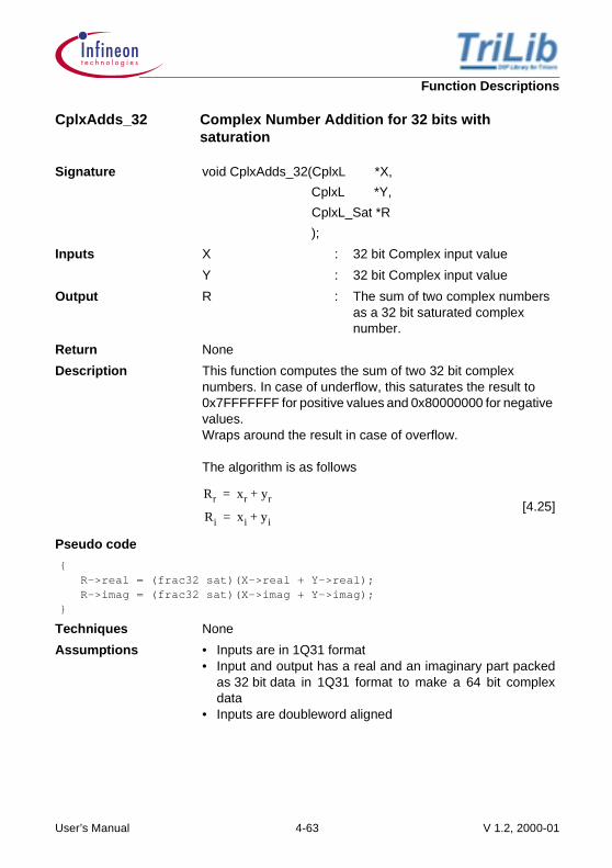
CplxAdds_32 Complex Number Addition for 32 bits with saturation
Signature void CplxAdds_32(CplxL *X,
CplxL *Y,
CplxL_Sat *R
);
Inputs X : 32 bit Complex input value
Y : 32 bit Complex input value
Output R : The sum of two complex numbers as a 32 bit saturated complex number.
Return None
Description This function computes the sum of two 32 bit complex numbers. In case of underflow, this saturates the result to 0x7FFFFFFF for positive values and 0x80000000 for negative values.Wraps around the result in case of overflow.
The algorithm is as follows
[4.25]
Pseudo code
{ R->real = (frac32 sat)(X->real + Y->real); R->imag = (frac32 sat)(X->imag + Y->imag);}
Techniques None
Assumptions • Inputs are in 1Q31 format• Input and output has a real and an imaginary part packed
as 32 bit data in 1Q31 format to make a 64 bit complexdata
• Inputs are doubleword aligned
Rr xr yr+=
Ri xi yi+=
User’s Manual 4-63 V 1.2, 2000-01

Function Descriptions
Memory Note
Figure 4-13 Complex number addition for 32 bits with saturation
Example Trilib\Example\Tasking\CplxArith\expCplx.c, expCplx.cpp
Trilib\Example\GreenHills\CplxArith\expCplx.cpp,expCplx.c
Trilib\Example\GNU\CplxArith\expCplx.c
Cycle Count 4+2
Code Size 22 bytes
CplxAdds_32 Complex Number Addition for 32 bits with saturation (cont’d)
63 31 0 63 31 0
+
+
Real Imaginary Real Imaginary
63 31 0
Real Imaginary
Sat Sat
User’s Manual 4-64 V 1.2, 2000-01

Function Descriptions
CplxSub_32 Complex Number Subtraction for 32 bits
Signature void CplxSub_32(CplxL *X,
CplxL *Y,
CplxL *R
);
Inputs X : 32 bit Complex input value
Y : 32 bit Complex input value
Output R : The difference of two complex numbers as a 32 bit complex number
Return None
Description This function computes the difference of two 32 bit complex numbers. Wraps around the result in case of overflow.The algorithm is as follows.
[4.26]
Pseudo code
{ R->real = X->real - Y->real; R->imag = X->imag - Y->imag;}
Techniques None
Assumptions • Inputs are in 1Q31 format• Input and output has a real and an imaginary part packed
as 32 bit data in 1Q31 format to make a 64 bit complexdata
• Inputs are doubleword aligned
Rr xr yr–=
Ri xr yi–=
User’s Manual 4-65 V 1.2, 2000-01

Function Descriptions
Memory Note
Figure 4-14 Complex number subtraction for 32 bits
Example Trilib\Example\Tasking\CplxArith\expCplx.c, expCplx.cpp
Trilib\Example\GreenHills\CplxArith\expCplx.cpp,expCplx.c
Trilib\Example\GNU\CplxArith\expCplx.c
Cycle Count 4+2
Code Size 22 bytes
CplxSub_32 Complex Number Subtraction for 32 bits (cont’d)
63 31 0 63 31 0
-
-
63 31 0
Real Imaginary Real Imaginary
Real Imaginary
User’s Manual 4-66 V 1.2, 2000-01

Function Descriptions
CplxSubs_32 Complex Number Subtraction for 32 bits with saturation
Signature void CplxSubs_32(CplxL *X,
CplxL *Y,
CplxL_Sat *R
);
Inputs X : 32 bit Complex input value
Y : 32 bit Complex input value
Output R : The difference of two complex numbers as a 32 bit saturated complex number
Return None
Description This function computes the difference of two 32 bit complex numbers. In case of underflow, this saturates the result to 0x7FFFFFFF for positive values and 0x80000000 for negative values. The algorithm is as follows.
[4.27]
Pseudo code
{ R->real = (frac32 sat)(X->real - Y->real); R->imag = (frac32 sat)(X->imag - Y->imag);}
Techniques None
Assumptions • Inputs are in 1Q31 format• Input and output has a real and an imaginary part packed
as 32 bit data in 1Q31 format to make a 64 bit complexdata
• Inputs are doubleword aligned
Rr xr yr–=
Ri xr yi–=
User’s Manual 4-67 V 1.2, 2000-01

Function Descriptions
Memory Note
Figure 4-15 Complex number subtraction for 32 bits with saturation
Example Trilib\Example\Tasking\CplxArith\expCplx.c, expCplx.cpp
Trilib\Example\GreenHills\CplxArith\expCplx.cpp,expCplx.c
Trilib\Example\GNU\CplxArith\expCplx.c
Cycle Count 4+2
Code Size 22 bytes
CplxSubs_32 Complex Number Subtraction for 32 bits with saturation (cont’d)
63 31 0 63 31 0
-
-
Real Imaginary Real Imaginary
63 31 0
Real Imaginary
Sat Sat
User’s Manual 4-68 V 1.2, 2000-01

Function Descriptions
CplxMul_32 Complex Number Multiplication for 32 bits
Signature void CplxMul_32(CplxL *X,
CplxL *Y,
CplxL *R
);
Inputs X : 32 bit Complex input value
Y : 32 bit Complex input value
Output R : The product of two complex numbers as a 32 bit complex number
Return None
Description This function computes the product of the two 32 bit complex numbers. Wraps around the result in case of overflow.
The complex multiplication is computed as follows.
Pseudo code
{ frac64 real; frac64 ima;
real = (frac64)((X->real * Y->real) - (X->imag * Y->imag)); //real part ima = (frac64)((X->real * Y->imag) + (X->imag * Y->real)); //imaginary part
R->real = (frac32)real; R->imag = (frac32)ima;}
Techniques None
Assumptions • Inputs are in 1Q31 format• Input and output has a real and an imaginary part packed
as 32 bit data in 1Q31 format to make a 64 bit complexdata
• Inputs are doubleword aligned
Rr xr yr xi yi×–×=
Ri xi yr xr yi×+×=
User’s Manual 4-69 V 1.2, 2000-01

Function Descriptions
Memory Note
Figure 4-16 Complex number multiplication for 32 bits
Example Trilib\Example\Tasking\CplxArith\expCplx.c, expCplx.cpp
Trilib\Example\GreenHills\CplxArith\expCplx.cpp,expCplx.c
Trilib\Example\GNU\CplxArith\expCplx.c
Cycle Count 13+2
Code Size 38 bytes
CplxMul_32 Complex Number Multiplication for 32 bits (cont’d)
63 31 0 63 31 0
+
63 31 0
Real Imaginary Real Imaginary
Real Imaginary
+
+
+
- +
User’s Manual 4-70 V 1.2, 2000-01

Function Descriptions
CplxMuls_32 Complex Number Multiplication for 32 bits with Saturation
Signature void CplxMuls_32(CplxL *X,
CplxL *Y,
CplxL_Sat *R
);
Inputs X : 32 bit Complex input value
Y : 32 bit Complex input value
Output R : The product of two complex numbers as a 32 bit complex number
Return None
Description This function computes the product of the two 32 bit complex numbers. In case of overflow, the result is saturated to 0x7FFFFFFF for positive overflow and 0x80000000 for negative underflow.
The complex multiplication is computed as follows.
Pseudo code
{ frac64 real; frac64 ima;
real = (frac64)((X->real * Y->real) - (X->imag * Y->imag)); //real part ima = (frac64)((X->real * Y->imag) + (X->imag * Y->real)); //imaginary part
R->real = (frac32 sat)real; R->imag = (frac32 sat)ima;}
Techniques None
Rr xr yr xi yi×–×=
Ri xi yr xr yi×+×=
User’s Manual 4-71 V 1.2, 2000-01

Function Descriptions
Assumptions • Inputs are in 1Q31 format• Input and output has a real and an imaginary part packed
as 32 bit data in 1Q31 format to make a 64 bit complexdata
• Inputs are doubleword aligned
Memory Note
Figure 4-17 Complex number multiplication for 32 bits with saturation
CplxMuls_32 Complex Number Multiplication for 32 bits with Saturation (cont’d)
63 31 0 63 31 0
+
63 31 0
Real Imaginary Real Imaginary
Real Imaginary
+
+
+
- +
Sat Sat
32 16 0
Real Imaginary
User’s Manual 4-72 V 1.2, 2000-01

Function Descriptions
Example Trilib\Example\Tasking\CplxArith\expCplx.c, expCplx.cpp
Trilib\Example\GreenHills\CplxArith\expCplx.cpp,expCplx.c
Trilib\Example\GNU\CplxArith\expCplx.c
Cycle Count 13+2
Code Size 38 bytes
CplxMuls_32 Complex Number Multiplication for 32 bits with Saturation (cont’d)
User’s Manual 4-73 V 1.2, 2000-01

Function Descriptions
CplxConj_32 Complex Number Conjugate for 32 bits
Signature void CplxConj_32(CplxL *X,
CplxL *R
);
Inputs X : 32 bit Complex input value
Output R : The conjugate of the complex number
Return None
Description This function finds the conjugate of a 32 bit complex number. Conjugate of a complex number is given by
[4.28]
Pseudo code
{ R->imag = 0.0 - X->imag; R->real = X->real;}
Techniques None
Assumptions • Input is in 1Q31 format• Input and output has a real and an imaginary part packed
as 32 bit data in 1Q31 format to make a 32 bit complexdata
• Inputs are doubleword aligned
R x iy+( ) x iy–= =
User’s Manual 4-74 V 1.2, 2000-01

Function Descriptions
Memory Note
Figure 4-18 Complex number conjugate for 32 bits
Example Trilib\Example\Tasking\CplxArith\expCplx.c, expCplx.cpp
Trilib\Example\GreenHills\CplxArith\expCplx.cpp,expCplx.c
Trilib\Example\GNU\CplxArith\expCplx.c
Cycle Count 2+2
Code Size 14 bytes
CplxConj_32 Complex Number Conjugate for 32 bits (cont’d)
63 31 0
Real Imaginary
63 31 0
Real Imaginary
Negate
User’s Manual 4-75 V 1.2, 2000-01

Function Descriptions
CplxMag_32 Magnitude of a Complex Number for 32 bits
Signature DataL CplxMag_32(CplxL X);
Inputs X : 32 bit Complex input value
Output None
Return The magnitude of the complex number as a 32 bit integer or fract
Description This function finds the magnitude of a 32 bit complex number.
The algorithm is as follows
[4.29]
Pseudo code
{ int indx; frac32 sat tempX; frac32 sat tempY; frac32 sat temp; frac32 sat sqrttab[15] = {0.999999999999, 0.7071067811865, 0.5, 0.3535533905933, 0.25, 0.1767766952966, 0.125, 0.08838834764832, 0.0625, 0.04419417382416, 0.03125, 0.02209708691208, 0.015625, 0.01104854345604, 0.0078125}; //Scale down the input by 2 X->real >>= 1; X->imag >>= 1;
//Power = real^2 + imag^2 tempX = (X->real * X->real); tempY = (X->imag * X->imag); tempX += tempY;
//Mag = sqrt(power); indx = exp1(tempX);//calculate the leading zero tempX = norm(tempX,indx); //normalise tempY = tempX >> 1;//y = x/2 tempY -= 0.5; //y = x/2 - 0.5 tempX = tempY + 0.9999999999999999; //sqrt(x) = y + 1
R x2
y2
+=
User’s Manual 4-76 V 1.2, 2000-01

Function Descriptions
temp = (tempY * tempY); //y^2 tempX -= temp >> 1;//sqrt(x) = (y + 1) - 0.5*y^2 temp= (temp*tempY);//y^3 tempX += temp >> 1;//sqrt(x) = (y + 1) - 0.5*y^2 + 0.5*y^3 temp = (temp * tempY); //y^4 tempX -= temp * 0.625; //sqrt(x) = (y + 1) - 0.5*y^2 + 0.5*y^3 - 0.625*y^4 temp = (temp * tempY); //y^5 tempX = tempX + (0.875 * temp); //sqrt(x) = (y + 1) - 0.5*y^2 + 0.5*y^3 // - 0.625*y^4 +0.875*y^5 tempX = tempX * sqrttab[indx]; return tempX;}
Techniques None
Assumptions • Inputs are doubleword aligned
Memory Note None
CplxMag_32 Magnitude of a Complex Number for 32 bits (cont’d)
User’s Manual 4-77 V 1.2, 2000-01

Function Descriptions
Implementation The real and imaginary parts of a complex number x+iy are scaled down by two to avoid overflow.
MAC is used to square the imaginary part and dual MAC is used to square the real part. Add these to give the power(x2+y2).
If the power is zero, then the whole computation is not done to save cycles. Power(x2+y2) is normalized and the exponent is used as the scale factor in the square root operation. The square root is computed using the taylor approximation series.
The taylor series for square root is as follows:Let Z = x2+y2
R = (Z + 1)/2
[4.30]
The final result sqrt(Z) is again rescaled using the scale factor as index of the square root table to give the magnitude.
Example Trilib\Example\Tasking\CplxArith\expCplx.c, expCplx.cpp
Trilib\Example\GreenHills\CplxArith\expCplx.cpp,expCplx.c
Trilib\Example\GNU\CplxArith\expCplxMag.c
Cycle Count 5262
(Best)(Worst)
Code Size 126 bytes
140 bytes (Data)
CplxMag_32 Magnitude of a Complex Number for 32 bits (cont’d)
sqrt Z( ) R 1 0.5R2
0.5R3
0.625R4
– 0.875R5
–+–+=
User’s Manual 4-78 V 1.2, 2000-01

Function Descriptions
CplxPhase_32 Phase of a Complex Number for 32 bits
Signature DataL CplxPhase_32(CplxL *X);
Inputs X : 32 bit Complex input value
Output None
Return The phase of a complex number as a 32 bit integer or fract
Description This function computes the phase of a complex number. The algorithm is as follows.
Phase = tan-1(y/x) [4.31]
Pseudo code
{ int indx; int flag; frac32 sat tempX; frac32 sat tempY; frac32 sat temp;
//Scale down the input by 2 X->real >>= 1; X->imag >>= 1;
//Power = real^2 + imag^2 if (X->real < 0) { tempX = -X->real; } else { tempX = X->real; } if (X->imag < 0) { tempY = -X->imag; } else { tempY = X->imag; }
User’s Manual 4-79 V 1.2, 2000-01

Function Descriptions
//Phase = arctan(imag/real) if (tempX <= tempY) { flag = 1; temp = tempX/tempY; } else { flag = 0; temp = tempY/tempX; }
indx = exp1(temp); //calculate the leading zero temp = norm(temp,indx); //normalise tempX = K5 * temp + K4; tempX = tempX * temp + K3; tempX = tempX * temp + K2; tempX = tempX * temp + K1; tempX = tempX * temp; if (flag == 1) { tempX = 0.5 - tempX; }
if (X->real < 0 && X->imag < 0) { tempX = tempX - 0.9999999999999; } else if (X->real < 0 && X->imag >= 0) { tempX = 0.9999999999999 - tempX; } else if (X->real >= 0 && X->imag < 0) { tempX = -tempX; }
return tempX;}
CplxPhase_32 Phase of a Complex Number for 32 bits (cont’d)
User’s Manual 4-80 V 1.2, 2000-01

Function Descriptions
Techniques None
Assumptions • Inputs are doubleword aligned
Memory Note None
Implementation The phase in a complex plane is the arctan(y/x), where y/x=z.
By Taylor series,
phase = tan-1(z) for Z<=1 [4.32]
or 0.5-tan-1(1/z) for z>1. [4.33]
If , the flag is set to indicate that Equation [4.32] to be computed, otherwise Equation [4.33] is computed.
After calculating y/x, the results are normalized. Then the arctan is calculated by using the Taylor approximation series is a polynomial expansion. This is as follows:
[4.34]
The final part of the processing extracts the sign of real and imaginary part and branches to appropriate quadrant.I quadrant : phase = arctan(y/x) radianII quadrant : phase = -arctan(y/x) radianIII quadrant: phase = arctan(y/x)- radianIV quadrant: phase = arctan(y/x) radian
The output of the function is given in radians and has to be scaled. The output is as follows+ = 0x7fffffff or 0.99999999- = 0x80000000 or -1.0
/2 is approximately equal to 0.5- /2 is approximately equal to -0.5
CplxPhase_32 Phase of a Complex Number for 32 bits (cont’d)
y x≤
arc z( )tan 0.318253z 0.003314z2
0.130908z3
–+=
+ 0.068542z4
0.009159z5
–
ππ
ππππ
User’s Manual 4-81 V 1.2, 2000-01

Function Descriptions
Example Trilib\Example\Tasking\CplxArith\expCplx.c, expCplx.cpp
Trilib\Example\GreenHills\CplxArith\expCplx.cpp,expCplx.c
Trilib\Example\GNU\CplxArith\expCplxPh.c
Cycle Count 7 7+44
(Best)(Worst)
Code Size 180 bytes
20 bytes (Data)
CplxPhase_32 Phase of a Complex Number for 32 bits (cont’d)
User’s Manual 4-82 V 1.2, 2000-01

Function Descriptions
CplxShift_32 Complex Number Shift for 32 bits
Signature void CplxShift_32(CplxL *X, CplxL *R, int shiftVal );
Inputs X : 32 bit Complex input value
shiftVal : shift value as a signed integer
Output R : Output value after the real and imaginary parts are shifted
Return None
Description This function performs shifting of a 32 bit complex number indicated by the shiftVal. Left shifting is done if the shiftVal is positive and Right shifting is done if shiftVal is negative.
The algorithm is as follows.
[4.35]
Pseudo code
{ if (Y < 0) { R->real = X->real >> Y; R->imag = X->imag >> Y; } else if (Y > 0) { R->real = X->real << Y; R->imag = X->imag << Y; } else { R->real = X->real; R->imag = X->imag; }}
Techniques None
Rr xr abs shiftVal( ) if shiftVal 0<( ),»=
else xr shiftVal«( )
Ri xi abs shiftVal( ) if shiftVal 0<( ),»=
else xi shiftVal«( )
User’s Manual 4-83 V 1.2, 2000-01

Function Descriptions
Assumptions • Inputs are doubleword aligned
Memory Note
Figure 4-19 Complex number shift for 32 bits
Example Trilib\Example\Tasking\CplxArith\expCplx.c, expCplx.cpp
Trilib\Example\GreenHills\CplxArith\expCplx.cpp,expCplx.c
Trilib\Example\GNU\CplxArith\expCplx.c
Cycle Count 3+2
Code Size 18 bytes
CplxShift_32 Complex Number Shift for 32 bits (cont’d)
63 31 0
63 31 0
Real Imaginary
Real Imag
....
0..0 0..0
.... 63 31 0
Real Imag
....
Sign Sign
Left shift if0<shift value<32
Right shift if-32<shift value< 0
....
User’s Manual 4-84 V 1.2, 2000-01

Function Descriptions
4.3 Vector Arithmetic Functions
A vector is a quantity that has both magnitude and direction. Many physical quantitiesare vectors, e.g., force, velocity and momentum. In order to compare vectors and tooperate on them mathematically, it is necessary to have some reference system thatdetermines scale and direction, such as Cartesian coordinates. A vector is frequentlysymbolized by its components with respect to the coordinate axis. The concept of avector can be extended to three or more dimensions.
4.3.1 Descriptions
The following vector arithmetic functions are described.
• Vector addition with saturation• Vector subtraction with saturation• Vector Dot product• Maximum element by index • Minimum element by index • Maximum element by value • Minimum element by value
User’s Manual 4-85 V 1.2, 2000-01

Function Descriptions
VecAdd Vector Operation - Addition of two vectors
Signature int VecAdd(DataS *X, DataS * Y, DataS_Sat *R, int nX );
Inputs X : Pointer to first vector components
Y : Pointer to second vector components
nX : Dimension of vector
Output R : Pointer to the sum of two vectors
Return None
Description This function finds the sum of two vectors.
If x and y are two vectors given by x = [x0, x1,....xN-1]T and y = [y0, y1,...,yN-1]T, their sum is given by
Ri = xi + yi (i = 0,1,..., N-1) [4.36]
Pseudo code
{ int i; for (i = 0;i < nX;i++) { R[i] = X[i] + Y[i]; //Add }}
Techniques None
Assumptions • The input vectors have the same dimension
User’s Manual 4-86 V 1.2, 2000-01

Function Descriptions
Memory Note
Figure 4-20 Vector Addition
VecAdd Vector Operation - Addition of two vectors (cont’d)
aX
X[1]
X[2]
.
.
.
.
X[0]
X[nX]
Y[1]
Y[2]
.
.
.
.
Y[0]
Y[nX]
R[1]
R[2]
.
.
.
.
R[0]
R[nX]
aR
aY+
+
+
+
User’s Manual 4-87 V 1.2, 2000-01
Function Descriptions
Implementation The Vector Add function adds with saturation the peer elements of two arrays and stores the result in the resultant array. It uses the packed Load/Store instruction to load 4 words of data simultaneously. It adds the 4 elements in one go and stores it into the result array. This is applicable for all the arrays with sizes equal to the multiples of 4 words. In case if the size is of odd or not the multiple of 4 words, it checks the remaining elements and correspondingly takes respective paths to execute the addition separately from the remaining words which is left out.
Example Trilib\Example\Tasking\Vectors\expVect.c, expVect.cpp
Trilib\Example\GreenHills\Vectors\expVect.cpp, expVect.c
Trilib\Example\GNU\Vectors\expVect.c
Cycle Count (Best)
(Worst)
Code Size 84 bytes
VecAdd Vector Operation - Addition of two vectors (cont’d)
7 5nX4
-------×+ 4 2+ +
7 5nX4
-------×+ 8 2+ +
User’s Manual 4-88 V 1.2, 2000-01

Function Descriptions
VecSub Vector Operation - Difference of two vectors
Signature int VecSub(DataS *X, DataS *Y, DataS_Sat *R, int nX );
Inputs X : Pointer to first vector components
Y : Pointer to second vector components
nX : Dimension of vector
Output R : Pointer to difference of two vectors
Return None
Description This function finds the difference of two vectors.
If x and y are two vectors given by x = [x0, x1,....xN-1]T and y = [y0, y1,...,yN-1]T, their sum is given by
Ri = xi - yi (i = 0,1,..., N-1) [4.37]
Pseudo code
{ int i; for (i = 0;i < nX;i++) { R[i] = X[i] - Y[i]; //Subtract }}
Techniques None
Assumptions • The input vectors have the same dimension
User’s Manual 4-89 V 1.2, 2000-01
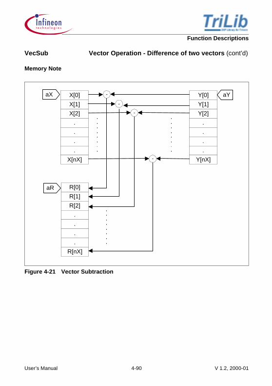
Function Descriptions
Memory Note
Figure 4-21 Vector Subtraction
VecSub Vector Operation - Difference of two vectors (cont’d)
aX
X[1]
X[2]
.
.
.
.
X[0]
X[nX]
Y[1]
Y[2]
.
.
.
.
Y[0]
Y[nX]
R[1]
R[2]
.
.
.
.
R[0]
R[nX]
aR
aY-
-
-
-
User’s Manual 4-90 V 1.2, 2000-01

Function Descriptions
Implementation The Vector Subtract function subtracts with saturation the X array data by the corresponding peer element of Y array and stores the result in the resultant array. It uses the packed Load/Store instruction to load 4 words of data simultaneously. It adds the 4 elements in one go and stores it into the result array. This is applicable for all the arrays with sizes equal to the multiples of 4 words. In case if the size is of odd or not the multiple of 4 words, it checks the remaining elements and correspondingly takes respective paths to execute the subtraction separately from the remaining words which is left out.
Example Trilib\Example\Tasking\Vectors\expVect.c, expVect.cpp
Trilib\Example\GreenHills\Vectors\expVect.cpp, expVect.c
Trilib\Example\GNU\Vectors\expVect.c
Cycle Count (Best)
(Worst)
Code Size 84 bytes
VecSub Vector Operation - Difference of two vectors (cont’d)
7 5nX4
-------×+ 4 2+ +
7 5nX4
-------×+ 8 2+ +
User’s Manual 4-91 V 1.2, 2000-01

Function Descriptions
VecDotPro Vector Operation - Dot Product of two vectors
Signature DataL VecDotPro(DataS *X,
DataS *Y,
int nX
);
Inputs X : Pointer to first vector components
Y : Pointer to second vector components
nX : Dimension of vectors
Output None
Return Dot product of the two vectors (48-bit output value convertedto 32-bit with saturation)
Description If x and y are two vectors of dimension N, their dot product is given by
[4.38]
Pseudo code
{ int i; frac64 product = 0;
for(i = 0;i < nX;i++) { product += (frac64) X[i](*)Y[i]; } //calculating the dot product return(frac32 sat)product; //Format the result to 32-bit saturated value}
Techniques • Use of MAC instructions• Intermediate results stored in a 64 bit register (16 guard
bits)• Dot product output is converted to 16 bit with saturation• Instruction ordering provided for zero overhead Load/Store
Assumptions • The input vectors have the same dimension
x y⋅ xi yi x0 y0 x1 y1 … xN 1– yN 1–⋅+ +⋅+⋅=⋅
i 0=
N 1–
∑=
User’s Manual 4-92 V 1.2, 2000-01

Function Descriptions
Memory Note
Figure 4-22 Dot product of two vectors
Implementation The Vector Dot Product function multiplies and accumulates the X array data by the corresponding peer element of Y array. It uses the madd.q instruction to do the multiply and accumulate the input data, the final result which is in 17Q47 format in a 64 bit register is converted to a 32 bit result and is saturated.
Example Trilib\Example\Tasking\Vectors\expVect.c, expVect.cpp
Trilib\Example\GreenHills\Vectors\expVect.cpp, expVect.c
Trilib\Example\GNU\Vectors\expVect.c
Cycle Count
Code Size 52 bytes
VecDotPro Vector Operation - Dot Product of two vectors (cont’d)
aX
X[1]
.
.
.
.
.
X[0]
X[Size]
Y[1]
.
.
.
.
.
Y[0]
Y[Size]
aY
acc
.
.
.
X[0].Y[0]= + X[1].Y[1]X[Size].Y[Size]
5 2 nX 1–[ ]× 5+ +
User’s Manual 4-93 V 1.2, 2000-01

Function Descriptions
VecMaxIdx Vector Operation - Maximum Element by Index of a vector
Signature int VecMaxIdx(DataS *X, int nX );
Inputs X : Pointer to the vector components
nX : Dimension of vector
Output None
Return The maximum element by index of the input vector
Description This function calculates the maximum element by index of avector. The input vector components are 16 bit real values.
Pseudo code
{ frac16 element = -1.0; int i;
for (i = 0;i < nX;i++) { if (element < X[i]) { element = X[i]; } } i = 0; while (element != X[i]) { i++; }
return i;}
Techniques None
Assumptions • Inputs are in 1Q15 format
User’s Manual 4-94 V 1.2, 2000-01

Function Descriptions
Memory Note
Figure 4-23 Maximum element by index
VecMaxIdx Vector Operation - Maximum Element by Index of a vector (cont’d)
X[1]
.
.
.
.
.
X[0]
X[size]
Max< x[0] Max=X[0], index=i
Max < x[1]
Max <x[size]
Max=X[1], index=i
Max=X[size], index=i
Return index
Yes
No
aX
User’s Manual 4-95 V 1.2, 2000-01

Function Descriptions
Implementation The Vector Maximum by Index function uses the max.h and eq.h instructions to optimally find the maximum value in the array. The max.h instruction checks the two 32 bit registers and returns the bigger 2 words among them into another register thereby does two comparison and movement of data in one go. Similarly the eq.h checks if the value is equal among the two registers, this is used here to find the greater value between the two words of a same 32 bit register finally, which is found to be in the maximum pair register after the computation of maximum element. Since the max.h does two comparisons, the loop count is reduced by half. The final part of the function is to calculate the index of the maximum element, this is done by initializing a index variable and is kept on incrementing until the maximum element found matches with one of the array’s element, odd array size is separately taken care.
Example Trilib\Example\Tasking\Vectors\expVect.c, expVect.cpp
Trilib\Example\GreenHills\Vectors\expVect.cpp, expVect.c
Trilib\Example\GNU\Vectors\expVect.c
Cycle Count
(Best)
(Worst)
Code Size 92 bytes
VecMaxIdx Vector Operation - Maximum Element by Index of a vector (cont’d)
4 2nX4
------- 1+× 3 212---×
2+ + + +
4 2nX4
------- 1+× 3 2nX2
-------× 2+ + + +
User’s Manual 4-96 V 1.2, 2000-01

Function Descriptions
VecMinIdx Vector Operation - Minimum Element by index of a vector
Signature int VecMinIdx(DataS *X, int nX );
Inputs X : Pointer to vector components
nX : Dimension of vector
Output None
Return The minimum element by index of the input vector
Description This function calculates the minimum element by index of avector. The input vector components are 16 bit real valuesand are halfword aligned.
Pseudo code
{ frac16 element = 0.99999999999999; int i;
for (i = 0;i < nX;i++) { if (element > X[i]) { element = X[i]; } } i = 0; while (element != X[i]) { i++; }
return i;}
Techniques None
Assumptions None
User’s Manual 4-97 V 1.2, 2000-01

Function Descriptions
Memory Note
Figure 4-24 Minimum element by index
VecMinIdx Vector Operation - Minimum Element by index of a vector (cont’d)
X[1]
.
.
.
.
.
X[0]
X[size]
Min>x[0] Min=X[0], index=i
Min>x[1]
Min>x[size]
Min=X[1], index=i
Min=X[size], index=i
Return index
Yes
No
aX
User’s Manual 4-98 V 1.2, 2000-01

Function Descriptions
Implementation The Vector Minimum by Index function uses the min.h and eq.h instructions to optimally find the minimum value in the array. The min.h instruction checks the two 32 bit registers and returns the smaller 2 words among them into another register thereby does two comparison and movement of data in one go. Similarly the eq.h checks if the value is equal among the two registers, this is used here to find the smaller value between the two words of a same 32 bit register finally, which is found to be in the minimum pair register after the computation of minimum element. Since the min.h does two comparisons, the loop count is reduced by half. The final part of the function is to calculate the index of the minimum element, this is done by initializing a index variable and is kept on incrementing until the minimum element found matches with one of the array’s element, odd array size is separately taken care.
Example Trilib\Example\Tasking\Vectors\expVect.c, expVect.cpp
Trilib\Example\GreenHills\Vectors\expVect.cpp, expVect.c
Trilib\Example\GNU\Vectors\expVect.c
Cycle Count(Best)
(Worst)
Code Size 98 bytes
VecMinIdx Vector Operation - Minimum Element by index of a vector (cont’d)
4 2nX4
------- 1+× 3 212---×
2+ + + +
4 2nX4
------- 1+× 3 2nX2
-------× 2+ + + +
User’s Manual 4-99 V 1.2, 2000-01

Function Descriptions
VecMaxVal Vector Operation - Maximum Element by value of a vector
Signature int VecMaxVal(DataS *X, int nX );
Inputs X : Pointer to vector components
nX : Dimension of vector
Output None
Return The maximum element by value of the input vector
Description This function calculates the maximum element by value of avector. The input vector components are 16 bit real valuesand are halfword aligned.
Pseudo code
{ frac16 element = -1.0; int i;
for (i = 0;i < nX ;i++) { if (element < X[i]) { element = X[i]; } } return element;}
Techniques None
Assumptions None
User’s Manual 4-100 V 1.2, 2000-01

Function Descriptions
Memory Note
Figure 4-25 Maximum element by value
VecMaxVal Vector Operation - Maximum Element by value of a vector (cont’d)
X[1]
.
.
.
.
.
X[0]
X[size]
Max<x[0] Max=X[0]
Max<x[1]
Max<x[size]
Max=X[1]
Max=X[size]
Return Max
Yes
No
aX
User’s Manual 4-101 V 1.2, 2000-01

Function Descriptions
Implementation The Vector Maximum by value function uses the max.h and eq.h instructions to optimally find the maximum value in the array. The max.h instruction checks the two 32 bit registers and returns the bigger 2 words among them into another register thereby does two comparison and movement of data in one go. Similarly the eq.h checks if the value is equal among the two registers, this is used here to find the greater value between the two words of a same 32 bit register finally, which is found to be in the maximum pair register after the computation of maximum element. Since the max.h does two comparisons, the loop count is reduced by half. It returns the maximum value among the two in the maximum element register.
Example Trilib\Example\Tasking\Vectors\expVect.c, expVect.cpp
Trilib\Example\GreenHills\Vectors\expVect.cpp, expVect.c
Trilib\Example\GNU\Vectors\expVect.c
Cycle Count(Best)
(Worst)
Code Size 56 bytes
VecMaxVal Vector Operation - Maximum Element by value of a vector (cont’d)
3 2nX4
------- 1+× 5+ +
3 2nX4
------- 1+× 7+ +
User’s Manual 4-102 V 1.2, 2000-01

Function Descriptions
VecMinVal Vector Operation - Minimum Element by value of a vector
Signature int VecMinVal(DataS *X, int nX );
Inputs X : Pointer to vector components
nX : Dimension of vector
Output None
Return The minimum element by value of the input vector
Description This function calculates the minimum element by value of avector. The input vector components are 16 bit real valuesand are halfword aligned.
Pseudo code
{ frac16 element = 0.999999999; int i;
for (i = 0;i < nX;i++) { if (element > X[i]) { element = X[i]; } } return element;}
Techniques None
Assumptions None
User’s Manual 4-103 V 1.2, 2000-01

Function Descriptions
Memory Note
Figure 4-26 Minimum element by value
VecMinVal Vector Operation - Minimum Element by value of a vector (cont’d)
X[1]
.
.
.
.
.
X[0]
X[size]
Min>x[0] Min=X[0]
Min>x[1]
Min>x[size]
Min=X[1]
Min=X[size]
Return Min
Yes
No
aX
User’s Manual 4-104 V 1.2, 2000-01

Function Descriptions
Implementation The Vector Minimum by value function uses the min.h and eq.h instructions to optimally find the minimum value in the array. The min.h instruction checks the two 32 bit registers and returns the smaller 2 words among them into another register thereby does two comparison and movement of data in one go. Similarly the eq.h checks if the value is equal among the two registers, this is used here to find the smaller value between the two words of a same 32 bit register finally, which is found to be in the minimum pair register after the computation of minimum element. Since the min.h does two comparisons, the loop count is reduced by half. It returns the minimum value among the two in the minimum element register.
Example Trilib\Example\Tasking\Vectors\expVect.c, expVect.cpp
Trilib\Example\GreenHills\Vectors\expVect.cpp, expVect.c
Trilib\Example\GNU\Vectors\expVect.c
Cycle Count(Best)
(Worst)
Code Size 56 bytes
VecMinVal Vector Operation - Minimum Element by value of a vector (cont’d)
3 2nX4
------- 1+× 5+ +
3 2nX4
------- 1+× 7+ +
User’s Manual 4-105 V 1.2, 2000-01

Function Descriptions
4.4 FIR Filters
4.4.1 Normal FIR
The FIR (Finite Impulse Response) filter, as its name suggests, will always have a finiteduration of non-zero output values for given finite duration of non-zero input values. FIRfilters use only current and past input samples, and none of the filter’s previous outputsamples, to obtain a current output sample value.
For causal FIR systems, the system function has only zeros (except for poles at z=0).The FIR filter can be realized in transversal, cascade and lattice forms. The implementedstructure is of transversal type, which is realized by a tapped delay line. In case of FIR,delay line stores the past input values. The input x(n) for the current calculation willbecome x(n-1) for the next calculation. The output from each tap is summed to generatethe filter output. For a general nH tap FIR filter, the difference equation is
[4.39]
where,
The filter coefficients, which decide the scaling of current and past input samples storedin the delay line, define the filter response.
The transfer function of the filter in Z-transform is
[4.40]
X(n) : the filter input for nth sample
R(n) : output of the filter for nth sample
Hi : filter coefficients
nH : filter order
R n( ) Hi X n i–( )⋅
i 0=
nH 1–
∑=
H z[ ] R z[ ]X z[ ]------------ Hi Z
i–⋅
i 0=
nH 1–
∑= =
User’s Manual 4-106 V 1.2, 2000-01

Function Descriptions
Figure 4-27 Block Diagram of the FIR Filter
4.4.1.1 Descriptions
The following Normal FIR filter functions are described.
• Normal, Arbitrary number of coefficients, Sample processing• Normal, Arbitrary number of coefficients, Block processing• Normal, coefficients - multiple of 4, Sample processing• Normal, coefficients - multiple of 4, Block processing
Delay Line
+
Z-1
X
Z-1
X XH0 H1 H nH-1
X(n)(Filter Input)
X(n) X(n-1) X(n-nH+1)
R(n)(Filter Output)
Z-1
User’s Manual 4-107 V 1.2, 2000-01

Function Descriptions
Fir_16 FIR Filter, Normal, Arbitrary number of coefficients, Sample processing
Signature DataS Fir_16(DataS X, DataS *H, cptrDataS *DLY );
Inputs X : Real input value
H : Pointer to Coeff-Buffer of size nH
DLY : With DSP Extension - Pointer to circular pointer of Delay-Buffer of size nH, where nH is the filter orderWithout DSP Extension - Pointer to Circ-Struct
Output DLY : Updated circular pointer with index set to the oldest value of the filter Delay-Buffer
Return R : Output value of the filter (48-bit value converted to 16-bit with saturation)
Description The implementation of FIR filter uses transversal structure (direct form). A single input is processed at a time and output for every sample is returned. The filter operates on 16-bit real input, 16-bit coefficients and gives 16-bit real output. The number of coefficients given by the user is arbitrary. Circular buffer addressing mode is used for delay line. Coefficient buffer is halfword aligned. Delay line buffer is doubleword aligned.
User’s Manual 4-108 V 1.2, 2000-01

Function Descriptions
Pseudo code
{ frac64 acc; //Filter Result int j,k=0; frac16circ *aDLY = &DLY; //ptr to Circ-ptr of Delay-Buffer
*DLY = X; //Store input value in Delay-Buffer at //the position of the oldest value acc = 0.0; if(nH%2 == 0) //even coefficients { //’n’ in the comments refers current instant //The index i,j of X(i),H(j)(in the comments) are valid //for first loop iteration //For each next loop i,j should be decremented and //incremented by 2 respectively.
for(j=0; j<nH/2; j++) { acc = acc + (frac64)(*(H+k) * (*(DLY+k)) + (*(H+k+1))* (*(DLY+k+1))); //acc += X(n)*H(0) + X(n-1)*H(1) k=k+2; }
} else //odd coefficients { //’n’ in the comments refers current instant //The index i,j of X(i),H(j)(in the comments) are valid //for first loop iteration. //For each next loop i,j should be decremented and //incremented by 1 respectively.
Fir_16 FIR Filter, Normal, Arbitrary number of coefficients, Sample processing (cont’d)
User’s Manual 4-109 V 1.2, 2000-01

Function Descriptions
for(j=0; j<nH; j++) { acc = acc + (frac64)(*(H+k) * (*(DLY+k))); //acc += X(n)*H(0) k++; }
}
DLY--; //Set DLY.index to the oldest value //in Delay-Buffer aDLY=&DLY; //store updated delay R = (frac16 sat)acc; //Format the filter output from 48-bit //to 16-bit saturated value
return R; //Filter output returned}
Techniques • Loop unrolling, two taps/loop if coefficients are even, elseone tap/loop
• Use of packed data Load/Store• Delay line implemented as circular buffer• Use of dual MAC instruction for even coefficients and MAC
instruction for odd coefficients• Intermediate results stored in 64 bit register (16 guard bits)• Instruction ordering for zero overhead Load/Store
Assumptions • Inputs, outputs, coefficients and delay line are in 1Q15format
• Filter order nH is not explicitly sent as an argument, insteadit is sent through the argument DLY as a size of circ-Delay-Buffer
Fir_16 FIR Filter, Normal, Arbitrary number of coefficients, Sample processing (cont’d)
User’s Manual 4-110 V 1.2, 2000-01

Function Descriptions
Memory Note
Figure 4-28 Fir_16
Fir_16 FIR Filter, Normal, Arbitrary number of coefficients, Sample processing (cont’d)
1Q15 1Q15
Delay-Buffer
aH
aDLY caDLY
H1
.
.
.
.
.
H0
HnH-1
Coeff-Buffer
MAC (oddnumber of
coefficients)
Dual MAC(even
number ofcoefficients)
doublewordaligned
X
.
X(n-nH + 1)
X(n)
X(n-1)
X(n-2)
.
.
.
halfwordaligned
User’s Manual 4-111 V 1.2, 2000-01

Function Descriptions
Implementation The FIR filter implemented structure is of transversal type, which is realized by a tapped delay line.
The FIR filter routine processes one sample at a time and returns the output of that sample. The input for which the output is to be calculated is sent as an argument to the function.
Implementation is different for even and odd coefficients.
Even number of coefficients:
TriCore’s load word instruction loads the two delay line values and two coefficients in one cycle. Dual MAC instruction performs a pair of multiplications and additions according to the equation
[4.41]
By using a dual MAC in the tap loop, the loop count is broughtdown by a factor of two. Here two taps are used during asingle pass and loop is unrolled for efficient pointer update ofdelay line. Thus loop is executed (nH/2-1) times.
Odd number of coefficients:
TriCore’s load halfword instruction loads one delay line value and one coefficient in one cycle. MAC instruction performs one multiplication and one addition according to the equation
[4.42]
By using a MAC in the tap loop, the loop count remains nH.Only one tap is used during a single pass and loop is unrolledfor efficient pointer update of delay line. Thus loop is executed(nH-1) times.
Fir_16 FIR Filter, Normal, Arbitrary number of coefficients, Sample processing (cont’d)
acc acc X n( ) H0 X n 1–( ) H1⋅+⋅+=
acc acc X n( ) H0⋅+=
User’s Manual 4-112 V 1.2, 2000-01

Function Descriptions
The filter output R(n) is 16-bit saturated equivalent of accwhen the tap loop is executed fully.
For delay line, circular addressing mode is used which helpsin efficient delay update. The size of the circular Delay-Bufferis equal to the filter order, i.e., the number of coefficients.Circular buffer needs doubleword alignment. There is norestriction on the number of coefficients.
Delay pointer in the memory note shows updated pointer aftertap loop is over. This points to the oldest value in the delay-buffer which is replaced by new input value.
Example Trilib\Example\Tasking\Filters\FIR\expFir_16.c, expFir_16.cppTrilib\Example\GreenHills\Filters\FIR\expFir_16.cpp, expFir_16.cTrilib\Example\GNU\Filters\FIR\expFir_16.c
Cycle Count With DSP Extensions
For even number of coefficients
Pre-kernel : 10
Kernel :
Post-kernel : 2+2
For odd number of coefficients
Pre-kernel : 8
Kernel :
Post-kernel : 2+2
Fir_16 FIR Filter, Normal, Arbitrary number of coefficients, Sample processing (cont’d)
nH2
------- 1– 2 2+×
nH 1–[ ] 2 2+×
User’s Manual 4-113 V 1.2, 2000-01
Function Descriptions
Without DSP Extensions
For even number of coefficients
Pre-kernel : 10
Kernel : same as With DSP Extensions
Post-kernel : 3+2
For odd number of coefficients
Pre-kernel : 8
Kernel : same as With DSP Extensions
Post-kernel : 3+2
Code Size 110 bytes
Fir_16 FIR Filter, Normal, Arbitrary number of coefficients, Sample processing (cont’d)
User’s Manual 4-114 V 1.2, 2000-01

Function Descriptions
FirBlk_16 FIR Filter, Normal, Arbitrary number of coefficients, Block processing
Signature void FirBlk_16(DataS *X, DataS *R, cptrDataS H, cptrDataS *DLY, int nX );
Inputs X : Pointer to Input-Buffer
R : Pointer to Output-Buffer
H : Circular pointer of Coeff-Buffer of size nH
DLY : With DSP Extension - Pointer to circular pointer of Delay-Buffer of size nH, where nH is the filter orderWithout DSP Extension - Pointer to Circ-Struct
nX : Size of Input-Buffer
Outputs DLY : Updated circular pointer with index set to the oldest value of the filter Delay-Buffer
R(nX) : Output-Buffer
Return None
Description The implementation of FIR filter uses transversal structure (direct form). The block of inputs are processed at a time and output for every sample is stored in the output array. The filter operates on 16-bit real input, 16-bit coefficients and gives 16-bit real output. The number of coefficients given by user is arbitrary. Circular buffer addressing mode is used for coefficients and delay line. Both coefficient buffer and delay line buffer are doubleword aligned. The input buffer and the output buffer are halfword aligned.
User’s Manual 4-115 V 1.2, 2000-01

Function Descriptions
Pseudo code
{ frac64 acc; //Filter Result int j,i,k; frac16circ *aDLY=&DLY; //ptr to Circ-ptr of Delay-Buffer
for(i=0; i<nX; i++) { *DLY = *X; //Store input value in Delay-Buffer at //the position of the oldest value acc = 0.0; if(nH%2 == 0) { // ’n’ in the comments refers current instant //The index i,j of X(i),H(j)(in the comments) are //valid for first loop iteration. //For each next loop i,j should be decremented //and incremented by 2 respectively.
for(j=0; j<nH/2; j++) { acc = acc + (frac64)(*(H+k) * (*(DLY+k)) + (*(H+k+1)) * (*(DLY+k+1))); //acc += X(n)*H(0) + X(n-1)*H(1) k=k+2; } } else { // ’n’ in the comments refers current instant //The index i,j of X(i),H(j)(in the comments) are //valid for first loop iteration. //For each next loop i,j should be decremented and //incremented by 1 respectively.
FirBlk_16 FIR Filter, Normal, Arbitrary number of coefficients, Block processing (cont’d)
User’s Manual 4-116 V 1.2, 2000-01

Function Descriptions
for(j=0; j<nH; j++) { acc = acc + (frac64)(*(H+k) * (*(DLY+k))); //acc += X(n)*H(0) k=k+1; } } DLY--; //Set DLY.index to the oldest value //in Delay-Buffer aDLY=&DLY; // store updated delay *R++ = (frac16 sat)acc; //Format the filter output from 48-bit //to 16-bit saturated value }//end of indata loop}
Techniques • Loop unrolling, two taps/loop if coefficients are even elseone tap/loop
• Use of packed data Load/Store• Delay line implemented as circular buffer• Coefficient buffer implemented as circular buffer• Use of dual MAC instruction for even number of coefficients
and MAC instructions for odd number of coefficients• Intermediate results stored in 64 bit register (16 guard bits)• Instruction ordering for zero overhead Load/Store
Assumptions • Inputs, outputs, coefficients and delay line are in 1Q15format
• Filter order nH is not explicitly sent as an argument, insteadit is sent through the argument DLY as a size of circ-Delay-Buffer
FirBlk_16 FIR Filter, Normal, Arbitrary number of coefficients, Block processing (cont’d)
User’s Manual 4-117 V 1.2, 2000-01

Function Descriptions
Memory Note
Figure 4-29 FirBlk_16
FirBlk_16 FIR Filter, Normal, Arbitrary number of coefficients, Block processing (cont’d)
Input-BufferOutput-Buffer
Delay-Buffer
Coeff-Buffer
aRaXX(1)
.
.
X(n)
X(n+1)
.
X(0)
.
R(1)
.
.
R(n)
R(n + 1)
.
R(0)
.
aDLYcaDLY
MAC (oddnumber of
coefficients)
H0
H1
.
.
.
HnH-1
1Q15
1Q15
1Q15
aHcaH
Dual MAC(even
number ofcoefficients)
doublewordaligned
doublewordaligned
halfwordaligned
halfwordaligned
.
X(n-nH+1)
X(n)
X(n-1)
X(n-2)
.
.
.
1Q15
User’s Manual 4-118 V 1.2, 2000-01

Function Descriptions
Implementation This FIR filter routine processes a block of input values at a time. The pointer to the input buffer is sent as an argument to the function. The output is stored in output buffer, the starting address of which is also sent as an argument to the function.
Implementation details are same as Fir_16, except that the Coeff-Buffer is also circular and needs doubleword alignment. The size of the Coeff-Buffer is equal to the filter order, i.e., the number of coefficients. Because of circular addressing used for Coeff-Buffer, at the end of the tap loop coeff-pointer always points to H0, i.e., first coefficient which is needed for next instant. An additional loop is needed to calculate the output for every sample in the buffer. Hence, this loop is repeated as many times as the size of the input buffer.
Example Trilib\Example\Tasking\Filters\FIR\expFirBlk_16.c, expFirBlk_16.cppTrilib\Example\GreenHills\Filters\FIR\expFirBlk_16.cpp, expFirBlk_16.cTrilib\Example\GNU\Filters\FIR\expFirBlk_16.c
Cycle Count With DSP Extensions
For even number of coefficients
Pre-loop : 9
Loop :
Post-loop : 1+2
For odd number of coefficients
Pre-loop : 6
Loop :
Post-loop : 1+2
FirBlk_16 FIR Filter, Normal, Arbitrary number of coefficients, Block processing (cont’d)
nX 5nH2
------- 1– 2 1+× 3+ +
×
+3
nX 5 nH 1–( ) 2 1+×[ ] 3+ +{ }×+3
User’s Manual 4-119 V 1.2, 2000-01

Function Descriptions
Without DSP Extensions
For even number of coefficients
Pre-loop : 11
Loop : same as With DSP Extensions
Post-Loop : 1+2
For odd number of coefficients
Pre-loop : 8
Loop : same as With DSP Extensions
Post-loop : 1+2
Code Size 178 bytes
FirBlk_16 FIR Filter, Normal, Arbitrary number of coefficients, Block processing (cont’d)
User’s Manual 4-120 V 1.2, 2000-01

Function Descriptions
Fir_4_16 FIR Filter, Normal, Coefficients - multiple of four, Sample processing
Signature DataS Fir_4_16(DataS X, DataS *H, cptrDataS *DLY );
Inputs X : Real input value
H : Pointer to Coeff-Buffer of size nH
DLY : With DSP Extension - Pointer to circular pointer of Delay-Buffer of size nH, where nH is the filter orderWithout DSP Extension - Pointer to Circ-Struct
Output DLY : Updated circular pointer with index set to the oldest value of the filter Delay-Buffer
Return R : Output value of the filter (48-bit value converted to 16-bit with saturation)
Description The implementation of FIR filter uses transversal structure (direct form). The single input is processed at a time and output for every sample is returned. The filter operates on 16-bit real input, 16-bit coefficients and gives 16-bit real output. The number of coefficients given by the user is multiple of four. Optimal implementation requires filter order to be multiple of four. Circular buffer addressing mode is used for delay line. Delay line buffer is doubleword aligned and it should be in internal memory. Coefficient-Buffer should be word aligned if it is in the external memory.
User’s Manual 4-121 V 1.2, 2000-01

Function Descriptions
Pseudo code
{ frac64 acc; //Filter Result int j,k; frac16circ *aDLY=&DLY; //ptr to Circ-ptr of Delay-Buffer
*DLY = X; //Store input value in Delay-Buffer at //the position of the oldest value acc = 0.0; //’n’ in the comments refers to current instant //The index i,j of X(i),H(j)(in the comments) are valid //for first loop iteration //For each next loop i,j should be decremented and //incremented by 4 respectively.
for(j=0; j<nH/4; j++) { acc = acc + (frac64)(*(H+k)*(*(DLY+k)) + (*(H+k+1)) * (*(DLY+k+1))); //acc += X(n)*H(0) + X(n-1)*H(1) acc = acc + (frac64)(*(H+k+2) * (*(DLY+k+2))+ (*(H+k+3)) * (*(DLY+k+3))); //acc += X(n-2)*H(2) + X(n-3)*H(3) k=k+4; }
DLY--; //Set DLY.index to the oldest value //in Delay-Buffer aDLY=&DLY; //store updated delay
R = (frac16 sat)acc; //Format the filter output from 48-bit //to 16-bit saturated value return R; //Filter output returned}
Techniques • Loop unrolling, four taps/loop• Use of packed data Load/Store• Delay line implemented as circular buffer• Use of dual MAC instructions• Intermediate results stored in 64-bit register (16 guard bits)• Instruction ordering for zero overhead Load/Store
Fir_4_16 FIR Filter, Normal, Coefficients - multiple of four, Sample processing (cont’d)
User’s Manual 4-122 V 1.2, 2000-01

Function Descriptions
Assumptions • Filter size must be multiple of 4 and minimum filter order iseight
• Inputs, outputs, coefficients and delay line are in 1Q15format
• Filter order nH is not explicitly sent as an argument, insteadit is sent through the argument DLY as a size of circ-Delay-Buffer
• Delay-Buffer is in internal memory
Memory Note
Figure 4-30 Fir_4_16
Fir_4_16 FIR Filter, Normal, Coefficients - multiple of four, Sample processing (cont’d)
aDLY
doublewordaligned
(Must be in IntMem)
Delay-Buffer Coeff-Buffer
Dual MAC
aH
caDLY
H1
.
.
.
.
.
H0
HnH-1
X
.
X(n-nH + 1)
X(n)
X(n-1)
X(n-2)
.
.
.
1Q151Q15
User’s Manual 4-123 V 1.2, 2000-01

Function Descriptions
Implementation The FIR filter implemented structure is of transversal type, which is realized by a tapped delay line.
The FIR filter routine processes one sample at a time and returns the output of that sample. The input for which the output is to be calculated is sent as an argument to the function.
TriCore’s load doubleword instruction loads four delay line values and four coefficients in one cycle. Each dual MAC instruction performs a pair of multiplications and additions according to the equation
[4.43]
Thus by using two dual MACs in the tap loop, the loop countis brought down by a factor of four. Here four taps are usedduring a single pass and loop is unrolled for efficient pointerupdate of delay line. Thus loop is executed (nH/4-1) times.The filter output R(n) is 16-bit saturated equivalent of accwhen the tap loop is fully executed.
To support load doubleword instruction, coeff-buffer shouldbe word aligned if it is in the external memory and halfwordaligned if it is in the internal memory. For delay line, circularaddressing mode is used which helps in efficient delayupdate. The size of the circular Delay buffer is equal to thefilter order, i.e., the number of coefficients. Circular bufferneeds doubleword alignment and to use load doublewordinstruction, size of the buffer should be multiple of eight bytes.This implies that the coefficients should be multiple of four.
Delay pointer in the memory note shows updated pointer aftertap loop is over. This points to the oldest value in the Delay-Buffer which is replaced by new input value.
Note: To Use load doubleword instruction for the delay linethe Delay-Buffer should be in internal memory only.
Fir_4_16 FIR Filter, Normal, Coefficients - multiple of four, Sample processing (cont’d)
acc acc X n( ) H0 X n 1–( ) H1⋅+⋅+=
User’s Manual 4-124 V 1.2, 2000-01

Function Descriptions
Example Trilib\Example\Tasking\Filters\FIR\expFir_4_16.c, expFir_4_16.cppTrilib\Example\GreenHills\Filters\FIR\expFir_4_16.cpp, expFir_4_16.cTrilib\Example\GNU\Filters\FIR\expFir_4_16.c
Cycle Count With DSP Extensions
Pre-kernel : 7
Kernel :
if nH > 8
if nH = 8
Post-kernel : 3+2
Without DSP Extensions
Pre-kernel : 7
Kernel : same as With DSP Extensions
Post-kernel : 4+2
Code Size 80 bytes
Fir_4_16 FIR Filter, Normal, Coefficients - multiple of four, Sample processing (cont’d)
nH4
------- 1– 2 2+×
nH4
------- 1– 2 1+×
User’s Manual 4-125 V 1.2, 2000-01

Function Descriptions
FirBlk_4_16 FIR Filter, Normal, Coefficients - multiple of four, Block processing
Signature void FirBlk_4_16(DataS *X, DataS *R, cptrDataS H, cptrDataS *DLY, int nX );
Inputs X : Pointer to Input-Buffer
R : Pointer to Output-Buffer
H : Circular pointer of Coeff-Buffer of size nH
DLY : With DSP Extension - Pointer to circular pointer of Delay-Buffer of size nH, where nH is the filter orderWithout DSP Extension - Pointer to Circ-Struct
nX : Size of Input-Buffer
Output DLY : Updated circular pointer with index set to the oldest value of the filter Delay-Buffer
R(nX) : Output-Buffer
Return None
Description The implementation of FIR filter uses transversal structure (direct form). The block of inputs are processed at a time and output for every sample is stored in the output array. The filter operates on 16-bit real input, 16-bit coefficients and gives 16-bit real output. The number of coefficients given by user is multiple of four. Optimal implementation requires filter order to be multiple of four. Circular buffer addressing mode is used for coefficients and delay line. Both coefficient buffer and delay line buffer are doubleword aligned. Input and output buffer are halfword aligned.
User’s Manual 4-126 V 1.2, 2000-01

Function Descriptions
Pseudo code
{ frac64 acc; //Filter Result int j,i,k; frac16circ *aDLY=&DLY; //Ptr to Circ-ptr of Delay-Buffer frac16circ *H; //Circ-ptr of Coeff-Buffer
for(i=0; i<nX; i++) { *DLY = *X; //Store input value in Delay-Buffer at //the position of the oldest value acc = 0.0; //’n’ in the comments refers to current instant //The index i,j of X(i),H(j)(in the comments) are //valid for first loop iteration //For each next loop i,j should be decremented //and incremented by 4 resp.
for(j=0; j<nH/4; j++) { acc = acc + (frac64)(*(H+k) * (*(DLY+k)) + (*(H+k+1)) * (*(DLY+k+1))); //acc += X(n)*H(0) + X(n-1)*H(1) acc = acc + (frac64)(*(H+k+2) * (*(DLY+k+2)) + (*(H+k+3)) * (*(DLY+k+3))); //acc += X(n-2)*H(2) + X(n-3)*H(3) k=k+4; }
DLY--; //Set DLY.index to the oldest value in Delay-Buffer aDLY = &DLY; //store updated delay *R++ = (frac16 sat)acc; //Format the filter output from 48-bit //to 16-bit saturated value } }
FirBlk_4_16 FIR Filter, Normal, Coefficients - multiple of four, Block processing (cont’d)
User’s Manual 4-127 V 1.2, 2000-01
Function Descriptions
Techniques • Loop unrolling, four taps/loop• Use of packed data Load/Store• Delay line implemented as circular buffer• Coefficient buffer implemented as circular buffer• Use of dual MAC instructions• Intermediate results stored in 64-bit register (16 guard bits)• Instruction ordering for zero overhead Load/Store
Assumptions • Filter order is a multiple of four and minimum filter order iseight
• Inputs, outputs, coefficients and delay line are in 1Q15format
• Filter order nH is not explicitly sent as an argument, insteadit is sent through the argument DLY as a size of circ-Delay-Buffer
• Delay-Buffer is in internal memory
FirBlk_4_16 FIR Filter, Normal, Coefficients - multiple of four, Block processing (cont’d)
User’s Manual 4-128 V 1.2, 2000-01

Function Descriptions
Memory Note
Figure 4-31 Fir_Blk_4_16
FirBlk_4_16 FIR Filter, Normal, Coefficients - multiple of four, Block processing (cont’d)
Input-Buffer Output-Buffer
Delay-Buffer
Coeff-Buffer
aRaXX(1)
.
.
X(n)
X(n+1)
.
X(0)
.
R(1)
.
.
R(n)
R(n + 1)
.
R(0)
.aDLYcaDLY
.
X(n-nH+1)
X(n)
X(n-1)
X(n-2)
.
.
.
DualMAC
H0
H1
.
.
.
HnH-1
1Q15
1Q15
1Q15
aHcaH
halfwordaligned
doublewordaligned
1Q15
doublewordaligned
halfwordaligned
(Must be in IntMem)
User’s Manual 4-129 V 1.2, 2000-01

Function Descriptions
Implementation This FIR filter routine processes a block of input values at a time. The pointer to the input buffer is sent as an argument to the function. The output is stored in output buffer, the starting address of which is also sent as an argument to the function.
Implementation details are same as Fir_4_16, except that the Coeff-Buffer is also circular and needs doubleword alignment. The size of the Coeff-Buffer is equal to the filter order, i.e., the number of coefficients. Because of circular addressing used for Coeff-Buffer, at the end of the tap loop coeff-pointer always points to H0, i.e., first coefficient which is needed for next instant. An additional loop is needed to calculate the output for every sample in the buffer. Hence, this loop is repeated as many times as the size of the input buffer.
Note: To Use load doubleword instruction for the delay linethe Delay-Buffer should be in internal memory only.
Example Trilib\Example\Tasking\Filters\FIR\expFirBlk_4_16.c, expFirBlk_4_16.cppTrilib\Example\GreenHills\Filters\FIR\expFirBlk_4_16.cpp, expFirBlk_4_16.cTrilib\Example\GNU\Filters\FIR\expFirBlk_4_16.c
Cycle Count With DSP Extensions
Pre-loop : 5
Loop :
Post-loop : 1+2
Without DSP Extensions
Pre-loop : 7
FirBlk_4_16 FIR Filter, Normal, Coefficients - multiple of four, Block processing (cont’d)
nX 5 2nH4
------- 1– 1+× 4+ +
×
+ 3
User’s Manual 4-130 V 1.2, 2000-01

Function Descriptions
4.4.2 Symmetric FIR
FIR filters with symmetrical Finite Impulse Response are called Symmetrical FIR filters.Such filters find use in signal processing applications such as speech processing wherelinear phase response is required to avoid phase distortion.
4.4.2.1 Descriptions
The following Symmetric FIR filter functions are described.
• Symmetric, Arbitrary number of coefficients, Sample processing• Symmetric, Arbitrary number of coefficients, Block processing• Symmetric, coefficients - multiple of 4, Sample processing• Symmetric, coefficients - multiple of 4, Block processing
Loop : same as With DSP Extensions
Post-loop : 1+2
Code Size 104 bytes
FirBlk_4_16 FIR Filter, Normal, Coefficients - multiple of four, Block processing (cont’d)
User’s Manual 4-131 V 1.2, 2000-01

Function Descriptions
FirSym_16 FIR Filter, Symmetric, Arbitrary number of coefficients, Sample processing
Signature DataS FirSym_16(DataS X, DataS *H, cptrDataS *DLY );
Inputs X : Real input value
H : Pointer to Coeff-Buffer of size nH/2
DLY : With DSP Extension - Pointer to circular pointer of Delay-Buffer of size nH, where nH is the filter orderWithout DSP Extension - Pointer to Circ-Struct
Output DLY : Updated circular pointer with index set to the oldest value of the filter Delay-Buffer
Return R : Output value of the filter (48-bit value converted to 16-bit with saturation)
Description The implementation of FIR filter uses transversal structure (direct form). A single input is processed at a time and output for that sample is returned. The filter operates on 16-bit real input, 16-bit coefficients and returns 16-bit real output. The number of coefficients given by the user is arbitrary and half of the filter order. Circular buffer addressing mode is used for delay line. Delay line buffer is double word aligned. Coeff-Buffer is halfword aligned. The Delay-Buffer is twice the size of Coeff-Buffer.
User’s Manual 4-132 V 1.2, 2000-01

Function Descriptions
Pseudo code
{ frac64 acc; //Filter Result int j,k; frac16circ *aDLY=&DLY1; //ptr to Circ-ptr of Delay-Buffer DLY2 = DLY1-1; //Ptr to X(n-nH+1) aDLY=&DLY2; //store index to the oldest value for next instant *DLY1 = X; //Store input value in Delay-Buffer at //the position of the oldest value for current instant acc = 0.0;
//The index i,j,k of X1(i),X2(j),H(k)(in the comments) //are valid for first loop iteration. //For each next loop i,j,k should be decremented, incremented and //incremented by 1 respectively. //’n’ in the comments refers to current instant
for(j=0; j<nH/2; j++) { acc = acc + (frac64)(*(H+k) * (*(DLY1+k))); //acc += X1(n) * H(0) acc = acc + (frac64)(*(H+k) * (*(DLY2-k))); //acc += X2(n-nH+1) * H(0) k=k+1; } DLY1=*aDLY; //Set DLY.index to the oldest value //in Delay-Buffer for next instant
R = (frac16 sat)acc; //Format the filter output from 48-bit //to 16-bit saturated value
return R; //Filter output is returned}
FirSym_16 FIR Filter, Symmetric, Arbitrary number of coefficients, Sample processing (cont’d)
User’s Manual 4-133 V 1.2, 2000-01

Function Descriptions
Techniques • Loop unrolling, two taps/loop• Use of packed data Load/Store• Delay line implemented as circular buffer• Use of MAC instructions• Intermediate results stored in 64-bit register (16 guard bits)• Instruction ordering for zero overhead Load/Store
Assumptions • Inputs, outputs, coefficients and delay line are in 1Q15format
• Filter order nH is not explicitly sent as an argument, insteadit is sent through the argument DLY as a size of circ-Delay-Buffer
Memory Note
Figure 4-32 FirSym_16
FirSym_16 FIR Filter, Symmetric, Arbitrary number of coefficients, Sample processing (cont’d)
Coeff-Buffer
aH
aDLY2caDLY2
MAC
1Q15doubleword
aligned
H0
H1
.
HnH/2 -1
aDLY1 caDLY1
1Q15
.
X(n-nH+2)
X(n-nH+1)
X(n)
X(n-1)
.
.
X(n-nH/2+1)
x(n-nH/2)
.
nH/2
MACX
halfwordaligned
Delay-Buffer
User’s Manual 4-134 V 1.2, 2000-01

Function Descriptions
Implementation The FIR filter implemented structure is of transversal type, which is realized by a tapped delay line.
The FIR filter routine processes one sample at a time and returns the output of that sample. The input for which the output is to be calculated is sent as an argument to the function.
TriCore’s load halfword instruction loads the one delay line value and one coefficient in one cycle each. For delay line, circular addressing mode is used. Two pointers are initialized for circular delay line, one points to X(n), which is incremented and the other points to X(n-nH+1), which is decremented to access all the delay line values. Each pointer accesses nH/2 values.
In a symmetric FIR filter, X(n) and X(n-nH+1) get multiplied with the same coefficient H0. This fact can be made use of to reduce the number of loads for coefficients. So, for the first pass in tap loop, one delay line pointer loads X(n) and the other pointer loads X(n-nH+1) by using load halfword instruction.
MAC instruction performs multiplication and addition. Two MACs are used in the tap loop, which for the first pass perform
[4.44]
Here two taps are used during a single pass and loop isunrolled to save cycle. Thus loop is executed (nH/2-1) times.The filter output R(n) is 16-bit saturated equivalent of accwhen the tap loop is fully executed.
As Delay-Buffer is circular, the delay line update is doneefficiently. The size of the circular Delay-Buffer is equal to thefilter order, i.e., twice the number of given coefficients.Circular buffer needs doubleword alignment and to use loadhalfword instruction, size of the buffer should be multiple oftwo bytes. There is no restriction on the number ofcoefficients.
FirSym_16 FIR Filter, Symmetric, Arbitrary number of coefficients, Sample processing (cont’d)
acc acc X n( ) H0⋅+=
acc acc X n nH– 1+( ) H0⋅+=
User’s Manual 4-135 V 1.2, 2000-01

Function Descriptions
Delay pointers in the memory note show updated pointers forthe next iteration. caDLY1 points to the oldest value in theDelay-Buffer which is replaced by new input value.
Example Trilib\Example\Tasking\Filters\FIR\expFirSym_16.c, expFirSym_16.cppTrilib\Example\GreenHills\Filters\FIR\expFirSym_16.cpp, expFirSym_16.cTrilib\Example\GNU\Filters\FIR\expFirSym_16.c
Cycle Count With DSP Extensions
Pre-kernel : 9
Kernel :
Post-kernel : 4+2
Without DSP Extensions
Pre-kernel : 9
Kernel : same as With DSP Extensions
Post-kernel : 5+2
Code Size 88 bytes
FirSym_16 FIR Filter, Symmetric, Arbitrary number of coefficients, Sample processing (cont’d)
nH2
------- 1– 3 2+×
User’s Manual 4-136 V 1.2, 2000-01

Function Descriptions
FirSymBlk_16 FIR Filter, Symmetric, Arbitrary number of coefficients, Block processing
Signature void FirSymBlk_16(DataS *X, DataS *R, DataS *H, cptrDataS *DLY, int nX );
Inputs X : Pointer to Input-Buffer of size nX
R : Pointer to Output-Buffer of size nX
H : Pointer to Coeff-Buffer of size nH/2
DLY : With DSP Extension - Pointer to circular pointer of Delay-Buffer of size nH, where nH is the filter orderWithout DSP Extension - Pointer to Circ-Struct
nX : Number of input samples
Outputs DLY : Updated circular pointer with index set to the oldest value of the filter Delay-Buffer
R(nX) : Output-Buffer
Return None
Description The implementation of FIR filter uses transversal structure (direct form). A block of inputs are processed at a time and output for every sample is stored in the output array. The filter operates on 16-bit real input, 16-bit coefficients and gives 16-bit real output. The number of coefficients given by the user is arbitrary and half of the filter order. Circular buffer addressing mode is used for delay line. Delay line buffer is doubleword aligned. Coefficient, Input and output buffer are halfword aligned. The Delay-Buffer is twice the size of Coeff-Buffer.
User’s Manual 4-137 V 1.2, 2000-01

Function Descriptions
Pseudo code
{ frac64 acc; //Filter Result int i,j,k; frac16circ *aDLY=&DLY1; //ptr to Circ-ptr of Delay-Buffer frac16 *H0; //Ptr to Coeff-Buffer H0 = H; //store coeff-buffer ptr DLY2 = DLY1-1; //Ptr to X(n-nH+1) aDLY = &DLY2; //store index to the oldest value of next instant *DLY1 = X; //Store input value in Delay-Buffer at //the position of the oldest value of current instant for(i=0; i<nX; i++) { acc = 0.0; k=0;
//The index i,j,k of X1(i),X2(j),H(k)(in the comments) //are valid for first loop iteration. // For each next loop i,j,k should be decremented, incremented and //incremented by 1 respectively. //’n’ in the comments refers to current instant
for(j=0; j<nH/2; j++) { acc = acc + (frac64)(*(H+k) * (*(DLY1+k))); //acc += X1(n) * H(0) acc = acc + (frac64)(*(H+k) * (*(DLY2-k))); //acc += X2(n-nH+1) * H(0) k=k+1; } DLY1 = *aDLY; //Set DLY.index to the oldest value in Delay-Buffer H = H0; //initialize coeff-ptr
*R++ = (frac16 sat)acc; //Format the filter output from 48-bit //to 16-bit saturated value }}
FirSymBlk_16 FIR Filter, Symmetric, Arbitrary number of coefficients, Block processing (cont’d)
User’s Manual 4-138 V 1.2, 2000-01

Function Descriptions
Techniques • Loop unrolling, two taps/loop• Use of packed data Load/Store• Delay line implemented as circular buffer• Use of MAC instructions• Intermediate results stored in 64-bit register (16 guard bits)• Instruction ordering for zero overhead Load/Store
Assumptions • Inputs, outputs, coefficients and delay line are in 1Q15format
• Filter order nH is not explicitly sent as an argument, insteadit is sent through the argument DLY as a size of circ-Delay-Buffer
FirSymBlk_16 FIR Filter, Symmetric, Arbitrary number of coefficients, Block processing (cont’d)
User’s Manual 4-139 V 1.2, 2000-01

Function Descriptions
Memory Note
Figure 4-33 FirSymBlk_16
FirSymBlk_16 FIR Filter, Symmetric, Arbitrary number of coefficients, Block processing (cont’d)
Input-Buffer Output-Buffer
Delay-Buffer
Coeff-Buffer
aR
R(1)
.
.
R(n)
R(n + 1)
.
R(0)
.
aH
aDLY2caDLY2
MAC
1Q15doubleword
aligned
H0
H1
.
HnH/2 -1
aDLY1 caDLY1
aX
1Q15 1Q15
1Q15
.
X(n-nH+2)
X(n-nH+1)
X(n)
X(n-1)
.
.
X(n-nH/2+1)
X(n-nH/2)
.
X(1)
.
.
X(n)
X(n+1)
.
X(0)
.
nH/2
MAC
halfwordaligned
halfwordaligned
halfwordaligned
User’s Manual 4-140 V 1.2, 2000-01

Function Descriptions
Implementation This symmetric FIR filter routine processes a block of input values at a time. The pointer to the input buffer is sent as an argument to the function. The output is stored in output buffer, the starting address of which is also sent as an argument to the function.
Implementation details are same as FirSym_16, except that the Coeff-Buffer pointer is stored for next iteration and an additional loop is needed to calculate the output for every sample in the buffer. Hence, this loop is repeated as many times as the size of the input buffer.
Example Trilib\Example\Tasking\Filters\FIR\expFirSymBlk_16.c, expFirSymBlk_16.cppTrilib\Example\GreenHills\Filters\FIR\expFirSymBlk_16.cpp, expFirSymBlk_16.cTrilib\Example\GNU\Filters\FIR\expFirSymBlk_16.c
Cycle Count Pre-loop : 4
Loop :
Post-loop : 0+2
Code Size 112 bytes
FirSymBlk_16 FIR Filter, Symmetric, Arbitrary number of coefficients, Block processing (cont’d)
nX 8 3nH2
------- 1– 1+× 5+ +
×
+3
User’s Manual 4-141 V 1.2, 2000-01

Function Descriptions
FirSym_4_16 FIR Filter, Symmetric, Coefficients - multiple of four, Sample processing
Signature DataS FirSym_4_16(DataS X, DataS *H, cptrDataS *DLY );
Inputs X : Real input value
H : Pointer to Coeff-Buffer of size nH/2
DLY : With DSP Extension - Pointer to circular pointer of Delay-Buffer of size nH, where nH is the filter orderWithout DSP Extension - Pointer to Circ-Struct
Output DLY : Updated circular pointer with index set to the oldest value of the filter Delay-Buffer
Return R : Output value of the filter (48-bit value converted to 16-bit with saturation)
Description The implementation of FIR filter uses transversal structure (direct form). A single input is processed at a time and output for that sample is returned. The filter operates on 16-bit real input, 16-bit coefficients and returns 16-bit real output. The filter order should be a multiple of four. Therefore number of coefficients given by the user should be even and half of the filter order. Optimal implementation requires filter order to be multiple of four. Circular buffer addressing mode is used for delay line. Delay line buffer is double word aligned. Coefficient buffer is halfword aligned. The Delay-Buffer is twice the size of Coeff-Buffer.
User’s Manual 4-142 V 1.2, 2000-01

Function Descriptions
Pseudo code
{ frac64 acc; //Filter Result int j,k; frac16circ *aDLY=&DLY1; //ptr to Circ-ptr of Delay-Buffer DLY2 = DLY1-1; aDLY=&DLY2; //store index to the oldest value for next instant DLY2 = DLY2-1; //Ptr to X(n-nH+2) *DLY1 = X; //Store input value in Delay-Buffer at //the position of the oldest value acc = 0.0;
//The index i,j,k of X1(i),X2(j),H(k)(in the comments) //are valid for first loop iteration. //For each next loop i,j,k should be decremented,incremented and //incremented by 2 resp. //’n’ in the comments refers to current instant for(j=0; j<nH/2; j++) { acc = acc + (frac64)(*(H+k) * (*(DLY1+k)) + (*(H+k+1)) * (*(DLY1+k+1))); //acc += X1(n) * H(0) + X1(n-1) * H(1) acc = acc + (frac64)(*(H+k) * (*(DLY2-k)) + (*(H+k+1)) * (*(DLY2-k-1))); //acc += X2(n-nH+1) * H(0) + X2(n-nH+2) * H(1) || k=k+2; } DLY1=*aDLY; //Set DLY.index to the oldest value //in Delay-Buffer for next instant
R = (frac16 sat)acc; //Format the filter output from 48-bit //to 16-bit saturated value
return R; //Filter output is returned}
FirSym_4_16 FIR Filter, Symmetric, Coefficients - multiple of four, Sample processing (cont’d)
User’s Manual 4-143 V 1.2, 2000-01

Function Descriptions
Techniques • Loop unrolling, four taps/loop• Use of packed data Load/Store• Delay line implemented as circular buffer• Use of dual MAC instructions• Intermediate results stored in 64-bit register (16 guard bits)• Instruction ordering for zero overhead Load/Store
Assumptions • Filter order is a multiple of four• Inputs, outputs, coefficients and delay line are in 1Q15
format • Filter order nH is not explicitly sent as an argument, instead
it is sent through the argument DLY as a size of circ-Delay-Buffer
Memory Note
Figure 4-34 FirSym_4_16
FirSym_4_16 FIR Filter, Symmetric, Coefficients - multiple of four, Sample processing (cont’d)
Delay-Buffer
Coeff-Buffer
aH
aDLY2 caDLY2
MAC
1Q15doubleword
aligned
H0
H1
.
HnH/2 -1
aDLY1 caDLY1
1Q15
.
X(n-nH+2)
X(n-nH+1)
X(n)
X(n-1)
.
.
X(n-nH/2+1)
x(n-nH/2)
.
nH
MACX
halfwordaligned
User’s Manual 4-144 V 1.2, 2000-01

Function Descriptions
Implementation The FIR filter implemented structure is of transversal type, which is realized as a tapped delay line.
The FIR filter routine processes one sample at a time and returns the output of that sample. The input for which the output is to be calculated is sent as an argument to the function.
TriCore’s load word instruction loads the two delay line values and two coefficients in one cycle. For delay line, circular addressing mode is used. Two pointers are initialized for circular delay line, one points to X(n), which is incremented and the other points to X(n-nH+2), which is decremented to access all the delay line values. Each pointer accesses nH/2 values.
In a symmetric FIR filter, X(n) and X(n-nH+1) get multiplied with the same coefficient H0. This fact can be made use of to reduce the number of loads for coefficients. So, for the first pass in tap loop, one delay line pointer loads X(n), X(n-1) and the other pointer loads X(n-nH+1), X(n-nH+2) by using load word instruction.
Dual MAC instruction performs a pair of multiplication and additions. Two dual MACs are used in the tap loop, which for the first pass perform
[4.45]
Here four taps are used during a single pass and loop isunrolled to save cycle. Thus loop is executed (nH/4-1) times.The filter output R(n) is 16-bit saturated equivalent of accwhen the tap loop is executed fully.
FirSym_4_16 FIR Filter, Symmetric, Coefficients - multiple of four, Sample processing (cont’d)
acc acc X n( ) H0 X n 1–( ) H1⋅+⋅+=
acc acc X n nH– 1+( ) H0 X n nH– 2+( ) H1⋅+⋅+=
User’s Manual 4-145 V 1.2, 2000-01

Function Descriptions
As Delay-Buffer is circular, the delay line update is doneefficiently. The size of the circular Delay-Buffer is equal to thefilter order, i.e., twice the number of given coefficients.Circular buffer needs doubleword alignment and to use loadword instruction, size of the buffer should be multiple of fourbytes. The number of coefficients given should be even,which means the filter order is a multiple of four.
Delay pointers in the memory note show updated pointers forthe next iteration. caDLY1 points to the oldest value in theDelay-Buffer which is replaced by new input value.
Example Trilib\Example\Tasking\Filters\FIR\expFirSym_4_16.c, expFirSym_4_16.cppTrilib\Example\GreenHills\Filters\FIR\expFirSym_4_16.cpp, expFirSym_4_16.cTrilib\Example\GNU\Filters\FIR\expFirSym_4_16.c
Cycle Count With DSP Extensions
Pre-kernel : 10
Kernel :
if nH > 8
if nH = 8
Post-Kernel : 4+2
Without DSP Extensions
Pre-kernel : 10
Kernel : same as With DSP Extensions
FirSym_4_16 FIR Filter, Symmetric, Coefficients - multiple of four, Sample processing (cont’d)
nH4
------- 1– 3 2+×
nH4
------- 1– 3 1+×
User’s Manual 4-146 V 1.2, 2000-01

Function Descriptions
Post-kernel : 5+2
Code Size 92 bytes
FirSym_4_16 FIR Filter, Symmetric, Coefficients - multiple of four, Sample processing (cont’d)
User’s Manual 4-147 V 1.2, 2000-01

Function Descriptions
FirSymBlk_4_16 FIR Filter, Symmetric, Coefficients - multiple of 4, Block processing
Signature void FirSymBlk_4_16(DataS *X, DataS *R, DataS *H, cptrDataS *DLY, int nX );
Inputs X : Pointer to Input-Buffer
R : Pointer to Output-Buffer
H : Pointer to Coeff-Buffer of size nH/2
DLY : With DSP Extension - Pointer to circular pointer of Delay-Buffer of size nH, where nH is the filter orderWithout DSP Extension - Pointer to Circ-Struct
nX : Size of Input-Buffer
Output DLY : Updated circular buffer with index set to the oldest value of the filter Delay-Buffer
R : Output-Buffer
Return None
Description The implementation of FIR filter uses transversal structure(direct form). A block of inputs are processed at a time andoutput for every sample is stored in the output array. The filteroperates on 16-bit real input, 16-bit coefficients and gives 16-bit real output. The filter order should be a multiple of four.Therefore the number of coefficients given by the user shouldbe even and half of the filter order. Optimal implementationrequires filter order to be multiple of four. Circular bufferaddressing mode is used for delay line. Delay line buffer isdoubleword aligned. Input, output and coefficient buffer arehalfword aligned. The Delay-Buffer is twice the size of Coeff-Buffer.
User’s Manual 4-148 V 1.2, 2000-01
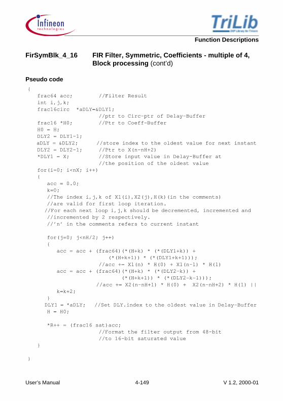
Function Descriptions
Pseudo code
{ frac64 acc; //Filter Result int i,j,k; frac16circ *aDLY=&DLY1; //ptr to Circ-ptr of Delay-Buffer frac16 *H0; //Ptr to Coeff-Buffer H0 = H; DLY2 = DLY1-1; aDLY = &DLY2; //store index to the oldest value for next instant DLY2 = DLY2-1; //Ptr to X(n-nH+2) *DLY1 = X; //Store input value in Delay-Buffer at //the position of the oldest value for(i=0; i<nX; i++) { acc = 0.0; k=0; //The index i,j,k of X1(i),X2(j),H(k)(in the comments) //are valid for first loop iteration. //For each next loop i,j,k should be decremented, incremented and //incremented by 2 respectively. //’n’ in the comments refers to current instant
for(j=0; j<nH/2; j++) { acc = acc + (frac64)(*(H+k) * (*(DLY1+k)) + (*(H+k+1)) * (*(DLY1+k+1))); //acc += X1(n) * H(0) + X1(n-1) * H(1) acc = acc + (frac64)(*(H+k) * (*(DLY2-k)) + (*(H+k+1)) * (*(DLY2-k-1))); //acc += X2(n-nH+1) * H(0) + X2(n-nH+2) * H(1) || k=k+2; } DLY1 = *aDLY; //Set DLY.index to the oldest value in Delay-Buffer H = H0;
*R++ = (frac16 sat)acc; //Format the filter output from 48-bit //to 16-bit saturated value }
}
FirSymBlk_4_16 FIR Filter, Symmetric, Coefficients - multiple of 4, Block processing (cont’d)
User’s Manual 4-149 V 1.2, 2000-01

Function Descriptions
Techniques • Loop unrolling, four taps/loop• Use of packed data Load/Store• Delay line implemented as circular buffer• Use of dual MAC instructions• Intermediate results stored in 64-bit register (16 guard bits)• Instruction ordering for zero overhead Load/Store
Assumptions • Inputs, outputs, coefficients and delay line are in 1Q15format
• Filter order nH is not explicitly sent as an argument, insteadit is sent through the argument DLY as a size of circ-Delay-Buffer
FirSymBlk_4_16 FIR Filter, Symmetric, Coefficients - multiple of 4, Block processing (cont’d)
User’s Manual 4-150 V 1.2, 2000-01

Function Descriptions
Memory Note
Figure 4-35 FirSymBlk_4_16
FirSymBlk_4_16 FIR Filter, Symmetric, Coefficients - multiple of 4, Block processing (cont’d)
Input-BufferOutput-Buffer
Delay-Buffer
Coeff-Buffer
aR
R(1)
.
.
R(n)
R(n + 1)
.
R(0)
.
aH
aDLY2 caDLY2
DualMAC
1Q15doubleword
aligned
H0
H1
.
HnH/2 -1
aDLY1 caDLY1
aX
1Q15
DualMAC
1Q15
1Q15
.
X(n-nH+2)
X(n-nH+1)
X(n)
X(n-1)
.
.
X(n-nH/2+1)
X(n-nH/2)
.
X(1)
.
.
X(n)
X(n+1)
.
X(0)
.
nH/2
halfwordaligned halfword
aligned
halfwordaligned
User’s Manual 4-151 V 1.2, 2000-01

Function Descriptions
4.4.3 Multirate Filters
Discrete time systems with unequal sampling rates at various parts of the system arecalled Multirate Systems. For sampling rate alterations, the basic sampling ratealteration devices are invariably employed together with lowpass digital filters. Filtershaving different sampling rates at input and output of filter are called Multirate Filters.The two types of multirate filtering processes are Decimation filtering and Interpolationfiltering.
Implementation This symmetric FIR filter routine processes a block of input values at a time. The pointer to the input buffer is sent as an argument to the function. The output is stored in output buffer, the starting address of which is also sent as an argument to the function.
Implementation details are same as FirSym_4_16, except that the Coeff-Buffer pointer is stored for next iteration and an additional loop is needed to calculate the output for every sample in the buffer. Hence, this loop is repeated as many times as the size of the input buffer.
Example Trilib\Example\Tasking\Filters\FIR\expFirSymBlk_4_16.c, expFirSymBlk_4_16.cppTrilib\Example\GreenHills\Filters\FIR\expFirSymBlk_4_16.cpp, expFirSymBlk_4_16.cTrilib\Example\GNU\Filters\FIR\expFirSymBlk_4_16.c
Cycle Count Pre-kernel : 4
Kernel :
Post-kernel : 0+2
Code Size 116 bytes
FirSymBlk_4_16 FIR Filter, Symmetric, Coefficients - multiple of 4, Block processing (cont’d)
nX 9 3nH4
------- 1– 1+× 5+ +
×
+ 1+2
User’s Manual 4-152 V 1.2, 2000-01

Function Descriptions
4.4.3.1 Decimating Filters
Decimation is equivalent to down sampling a discrete-time signal. It is used to eliminateredundant data, allowing more information to be stored, processed or transmitted in thesame amount of data.
Decimator or down sampler reduces the sampling rate by a factor of integer M.
Figure 4-36 Decimation/down Sampling Illustration
The sampling rate of a critically sampled discrete time signal with a spectrum occupyingthe full Nyquist range cannot be reduced any further since such a reduction will introducealiasing. Hence the bandwidth of a critically sampled signal must first be reduced bylowpass filtering before its sampling rate is reduced by a down sampler. The decimationalgorithm can be implemented using FIR or IIR filter structure. But generally, FIR is used.The overall system comprising of a lowpass filter followed by a down sampler ahead ofa lowpass FIR filter is called decimator or decimating FIR. Such a filter would give anoutput for every Mth input.
The decimating FIR filter is given by
[4.46]
Figure 4-37 Decimation Filter Block Diagram
4.4.3.2 Interpolating FIR Filters
Interpolation increases the sample rate of a signal inserting zeros between the samplesof input data. In practice, the zero-valued samples inserted by the up sampler arereplaced with appropriate non-zero values using some type of interpolation process in
MX[n]=Xa(nT) y[n]=Xa(nMT)
FT=1/T F’T=FT/M=1/T’
y m( ) h K( )x Mm K–( )
K 0=
N 1–
∑=
MH(Z)X[n] y[n]V[n]
User’s Manual 4-153 V 1.2, 2000-01

Function Descriptions
order that the new higher rate sequence be useful. This interpolation can be done bydigital lowpass filtering.
Figure 4-38 Interpolation/Down Sampling Illustration
The system comprising of up sampler followed by FIR lowpass filter which is used toremove the unwanted images in the spectra of up sampled signal is called InterpolatingFIR filter.
Figure 4-39 Interpolation Filter Block Diagram
The rate expander inserts If-1 zero valued samples after each input sample. Theresulting samples Xin[n] are lowpass filtered to produce output y(n), a smooth and antiimaged version of Xin[n]. The transfer function of interpolator H(k) incorporates a gain of1/If because the If-1 zeros inserted by the rate expander cause the energy of each inputto be spread over If output samples. The lowpass filter of interpolator uses a direct formFIR filter structure for computational efficiency. Output of an FIR filter is given by
[4.47]
where,
N-1 : the number of filter coefficients (taps)
Xin[n-k] : the rate expanded version of the input X[n]
LX[n]=Xa(nT) y[n]=Xa(n/LT)
FT=1/T F’T=FT.L=1/T’
H(Z)LX[n]
Xin[n]
y[n]
y n[ ] h k( )Xin n k–[ ]
k 0=
N 1–
∑=
User’s Manual 4-154 V 1.2, 2000-01

Function Descriptions
X[n] is related to Xin[n-k] by
for (n-k)=0,
Otherwise
4.4.3.3 Description
The following Multirate FIR filters are described.
• Decimation FIR• Interpolation FIR
Xin n k–[ ]X n k–( ) If⁄( )
0
= If 2If…±,±
User’s Manual 4-155 V 1.2, 2000-01

Function Descriptions
FirDec_16 Decimation FIR Filter
Signature void FirDec_16(DataS *X, DataS *R, cptrDataS H, cptrDataS *DLY, int nX, int Df );
Inputs X : Pointer to Input-Buffer
R : Pointer to Output-Buffer
H : Circular pointer of Coeff-Buffer of size nH
DLY : With DSP Extension - Pointer to circular pointer of Delay-Buffer of size nHWithout DSP Extension - Pointer to Circ-Struct
(nH) : Transferred as a part of Circular Pointer data type in a DLY parameter
nX : Size of Input-Buffer
Df : Decimation length
Outputs DLY : Updated circular pointer with index set to the oldest value of the filter Delay-Buffer
R(nX) : Output-Buffer
Return None
Description The implementation of Decimation FIR filter uses transversal structure (direct form). A block of inputs are processed at a time. The filter operates on 16-bit real input, 16-bit coefficients and gives 16-bit real output. Number of coefficients is arbitrary. If nX/Df is not an integer, the trailing samples are lost. Circular buffer addressing mode is used for coefficients and delay line. Both coefficient buffer and Delay-Buffer are doubleword aligned. Input and output buffers are halfword aligned.
User’s Manual 4-156 V 1.2, 2000-01

Function Descriptions
Pseudo code
{ frac64 acc; //Filter result int j,i,k; frac16circ *adly=&DLY; //Ptr to Circ-ptr of Delay-Buffer //macro macro FirDec EV_Coef, EV_Coef_Odd_Df { if EV_Coef==TRUE { //FIR filtering for(i=0; i<nX; i++) { *DLY = *X++; //Store input value in Delay-Buffer at //the position of the oldest value acc = 0.0; // ’n’ in the comments refers current instant //The index i,j of X(i),H(j)(in the comments) are //valid for first loop iteration. //For each next loop i,j should be decremented //and incremented by 2 respectively. for(j=0; j<nH/2; j++) { acc = acc + (frac64)(*(H+k) * (*(DLY+k)) + (*(H+k+1)) * (*(DLY+k+1))); //acc += X(n)*H(0) + X(n-1)*H(1) k=k+2; } DLY--; //(Df-1) values loaded into delay buffer before next output //calculation if (EV_Coef_Odd_Df==TRUE) { for(i=0;i<(Df-1)/2;i++) { *DLY-- = *X++; *DLY-- = *X++; } } else {
FirDec_16 Decimation FIR Filter
User’s Manual 4-157 V 1.2, 2000-01
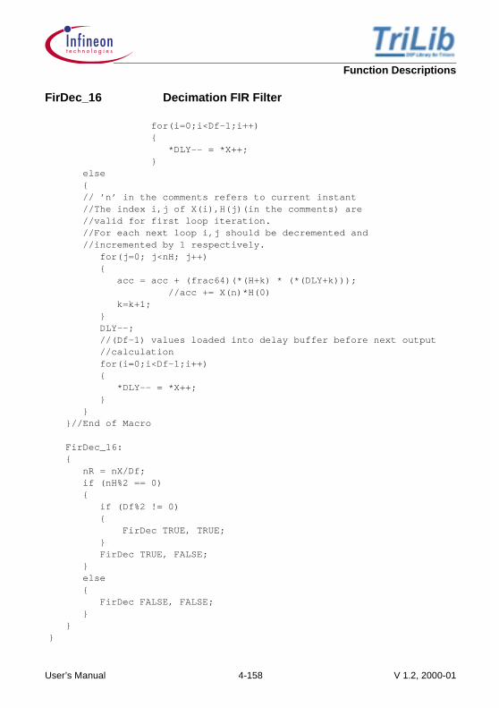
Function Descriptions
for(i=0;i<Df-1;i++) { *DLY-- = *X++; } else { // ’n’ in the comments refers to current instant //The index i,j of X(i),H(j)(in the comments) are //valid for first loop iteration. //For each next loop i,j should be decremented and //incremented by 1 respectively. for(j=0; j<nH; j++) { acc = acc + (frac64)(*(H+k) * (*(DLY+k))); //acc += X(n)*H(0) k=k+1; } DLY--; //(Df-1) values loaded into delay buffer before next output //calculation for(i=0;i<Df-1;i++) { *DLY-- = *X++; } } }//End of Macro
FirDec_16: { nR = nX/Df; if (nH%2 == 0) { if (Df%2 != 0) { FirDec TRUE, TRUE; } FirDec TRUE, FALSE; } else { FirDec FALSE, FALSE; } }}
FirDec_16 Decimation FIR Filter
User’s Manual 4-158 V 1.2, 2000-01

Function Descriptions
Techniques • Loop unrolling, two taps/loop if coefficients are even elseone tap/loop
• Use of packed data Load/Store• Delay line implemented as circular buffer• Coefficient buffer implemented as circular buffer• Intermediate results stored in 64-bit register • Instruction ordering for zero overhead Load/Store
Assumptions • Inputs, outputs, coefficients and delay line are in 1Q15format
• Filter order nH is not explicitly sent as an argument, insteadit is sent through the argument DLY as a size of circ-Delay-Buffer
FirDec_16 Decimation FIR Filter
User’s Manual 4-159 V 1.2, 2000-01

Function Descriptions
Memory Note
Figure 4-40 FirDec_16
FirDec_16 Decimation FIR Filter
Input-Buffer
Delay-Buffer
Coeff-Buffer
aXX(1)
.
.
X(n)
X(n+1)
.
X(0)
X(nX)aDLYcaDLY
.
X(n-nH+1)
X(n)
X(n-1)
X(n-2)
.
.
.
1Q15
1Q15
aHcaH
halfwordaligned
doublewordaligned
H1
.
.
HIn-1
HIn
.
H0
HnH-1
1Q15
doublewordaligned
Output-Buffer
aRR(1)
.
.
.
.
.
R(0)
R(nX/Df - 1)
1Q15
halfwordaligned
User’s Manual 4-160 V 1.2, 2000-01
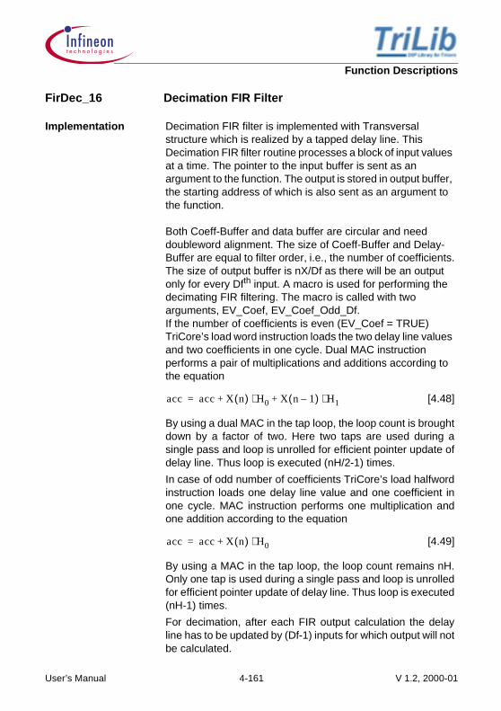
Function Descriptions
Implementation Decimation FIR filter is implemented with Transversal structure which is realized by a tapped delay line. This Decimation FIR filter routine processes a block of input values at a time. The pointer to the input buffer is sent as an argument to the function. The output is stored in output buffer, the starting address of which is also sent as an argument to the function.
Both Coeff-Buffer and data buffer are circular and need doubleword alignment. The size of Coeff-Buffer and Delay-Buffer are equal to filter order, i.e., the number of coefficients.The size of output buffer is nX/Df as there will be an output only for every Dfth input. A macro is used for performing the decimating FIR filtering. The macro is called with two arguments, EV_Coef, EV_Coef_Odd_Df. If the number of coefficients is even (EV_Coef = TRUE)TriCore’s load word instruction loads the two delay line values and two coefficients in one cycle. Dual MAC instruction performs a pair of multiplications and additions according to the equation
[4.48]
By using a dual MAC in the tap loop, the loop count is broughtdown by a factor of two. Here two taps are used during asingle pass and loop is unrolled for efficient pointer update ofdelay line. Thus loop is executed (nH/2-1) times.
In case of odd number of coefficients TriCore’s load halfwordinstruction loads one delay line value and one coefficient inone cycle. MAC instruction performs one multiplication andone addition according to the equation
[4.49]
By using a MAC in the tap loop, the loop count remains nH.Only one tap is used during a single pass and loop is unrolledfor efficient pointer update of delay line. Thus loop is executed(nH-1) times.
For decimation, after each FIR output calculation the delayline has to be updated by (Df-1) inputs for which output will notbe calculated.
FirDec_16 Decimation FIR Filter
acc acc X n( ) H0 X n 1–( ) H1⋅+⋅+=
acc acc X n( ) H0⋅+=
User’s Manual 4-161 V 1.2, 2000-01

Function Descriptions
If the number of coefficients is even and Df is odd,(EV_Coef_Odd_Df = TRUE) then the updation of delay linecan be done using TriCore’s load word instructions therebyreducing the loop count for the decimation loop by a factor oftwo else the load halfword instruction is used and the loop isexecuted (Df-1) times.
Thus the implementation is most optimal for the case of evencoefficient and odd Df.
Example Trilib\Example\Tasking\Filters\FIR\expFirDec_16.c, expFirDec_16.cppTrilib\Example\GreenHills\Filters\FIR\expFirDec_16.cpp, expFirDec_16.cTrilib\Example\GNU\Filters\FIR\expFirDec_16.c
Cycle Count For Macro FirDec
Mcall (TRUE,TRUE)
Pre-loop : 3
Loop :
Post-loop : 2
Mcall (TRUE,FALSE)
Pre-loop : 3
Loop :
Post-loop : 2
Mcall (TRUE,FALSE)
Pre-loop : 2
FirDec_16 Decimation FIR Filter
nXDf------- 5
nH2
------- 1– 2 5+ +×
+ Df 1–( ) 2⁄( )3 3 ] 2+ +
nXDf------- 5
nH2
------- 1– 2 5 Df 2( )+ + +×
+3 ] 2+
User’s Manual 4-162 V 1.2, 2000-01

Function Descriptions
Loop :
Post-loop : 2
where integer part of nX/Df is considered. The number ofcycles taken by the Loop should be reduced by nX/Df if eitherthe tap loop or the decimation loop gets executed only once.If both get executed only once then the total reduction innumber of cycles taken by the loop is 2(nX/Df) for all thecases.
For FirDec_16
With DSP Extensions
Even nH and odd Df
Even nH and even Df
Odd nH
where Mcall (X,Y) is the number of cycles taken by the macro when the arguments passed to it are X and Y.
FirDec_16 Decimation FIR Filter
nXDf------- 5 nH 1–( )2 5 Df 2( )+ + +[×
+3 ] 2+
31 Mcall TRUE TRUE,( ) 2 2+ + +
27 Mcall TRUE FALSE,( ) 2 2+ + +
28 Mcall FASLE FALSE,( ) 2 2+ + +
User’s Manual 4-163 V 1.2, 2000-01

Function Descriptions
Without DSP Extensions
Even nH and odd Df
Even nH and even Df
Odd nH
where Mcall (X,Y) is the number of cycles taken by the macro when the arguments passed to it are X and Y.
Code Size 308 bytes
33 Mcall TRUE TRUE,( ) 2 2+ + +
29 Mcall TRUE FALSE,( ) 2 2+ + +
30 Mcall FALSE FALSE,( ) 2 2+ + +
User’s Manual 4-164 V 1.2, 2000-01

Function Descriptions
FirInter_16 Interpolation FIR Filter
Signature void FirInter_16(DataS *X, DataS *R, cptrDataS H, cptrDataS *DLY, int nX, int If );
Inputs X : Pointer to Input-Buffer
R : Pointer to Output-Buffer
H : Circular pointer of Coeff-Buffer of size nH
DLY : With DSP Extension - Pointer to circular pointer of Delay-Buffer of size nHWithout DSP Extension - Pointer to Circ-Struct
(nH) : Transferred as a part of Circular Pointer data type in a DLY parameter
nX : Size of Input-Buffer
If : Interpolation length
Outputs DLY : Updated circular pointer with index set to the oldest value of the filter Delay-Buffer
R(nX) : Output-Buffer
Return None
Description The implementation of Interpolation FIR filter uses transversal structure (direct form). The block of inputs are processed at a time and output for every sample is stored in the output array. The filter operates on 16-bit real input, 16-bit coefficients and gives 16-bit real output. The number of coefficients given by user are arbitrary, but nX/If must be an integer. Circular buffer addressing mode is used for coefficients and delay line. Both coefficient buffer and delay line buffer are doubleword aligned. Input and output buffer are halfword aligned.
User’s Manual 4-165 V 1.2, 2000-01

Function Descriptions
Pseudo code
{ frac64 acc; //Filter result int i,j,k,l; frac16 circ*aDLY=DLY //Ptr to Circ-Ptr of Delay-Buffer if ((nH/If)%2 == 0) { for (i=0;i<nX;i++) { *DLY=*X //store input value in Delay-Buffer at the //position of the oldest value acc = 0.0; l = 0; for (j=0;j<If;j++) { // ’n’ in the comments refers current instant //The index i,j of X(i),H(j)(in the comments) are //valid for first loop iteration. //For each next loop i,j should be decremented and //incremented by 1 respectively. for (k=0;k<nH/2If;k++) { m = 0; acc = acc + (frac64)(*(H+l+m)*(*DLY+k)) + (*(H+l+m+1)* (*(DLY+k+1))); //acc = X(n)*H(0)+X(n-1)*H(If) m = m + If; k = k + 2; }//(nH/2If) loop l++; *R++ = (frac16 sat)acc; //format the filter output from 48-bit to 16-bit //saturated value }//(If) loop DLY--; }//nX loop }//If else {
FirInter_16 Interpolation FIR Filter (cont’d)
User’s Manual 4-166 V 1.2, 2000-01

Function Descriptions
for (i=0;i<nX;i++) { *DLY=*X //store input value in Delay-Buffer at the //position of the oldest value acc = 0.0; l = 0; for (j=0;j<If;j++) { // ’n’ in the comments refers current instant //The index i,j of X(i),H(j)(in the comments) are //valid for first loop iteration. //For each next loop i,j should be decremented and //incremented by 1 respectively. for (k=0;k<nH/If;k++) { m = 0; acc = acc + (frac64)(*(H+l+m)*(*DLY+k)) //acc = X(n)*H(0)+X(n-1)*H(If) m = m + If; k = k + 1; }//(nH/If) loop l++; *R++ = (frac16 sat)acc; //format the filter output from 48-bit to 16-bit //saturated value }//(If) loop DLY--; }//nX loop aDLY = DLY; //store updated delay }//else loop}
Techniques • Loop unrolling, one tap/loop if (nH/If) is odd and twotaps/loop if even
• Use of packed data Load/Store• Delay line implemented as circular buffer• Coefficient buffer implemented as circular buffer• Intermediate results stored in 64-bit register • Instruction ordering for zero overhead Load/Store
FirInter_16 Interpolation FIR Filter (cont’d)
User’s Manual 4-167 V 1.2, 2000-01

Function Descriptions
Assumptions • Inputs, outputs, coefficients and delay line are in 1Q15format
• Filter order nH is not explicitly sent as an argument, insteadit is sent through the argument DLY as a size of circ-Delay-Buffer
• The size of circ-Delay-Buffer is nH/If and it should beinteger
FirInter_16 Interpolation FIR Filter (cont’d)
User’s Manual 4-168 V 1.2, 2000-01

Function Descriptions
Memory Note
Figure 4-41 FirInter_16
FirInter_16 Interpolation FIR Filter (cont’d)
Input-BufferOutput-Buffer
Delay-Buffer
Coeff-Buffer
aRaXX(1)
.
.
X(n)
X(n+1)
.
X(0)
.
R(1)
.
.
Rf-1
Rf
.
R(0)
.aDLYcaDLY
.
X(n-nH+1)
X(n)
X(n-1)
X(n-2)
.
.
.
1Q15
1Q15
aHcaH
halfwordaligned
doublewordaligned
1Q15
halfwordaligned
H1
.
.
Hf-1
Hf
.
H0
HnH-1
1Q15
doublewordaligned
User’s Manual 4-169 V 1.2, 2000-01

Function Descriptions
Implementation Interpolation FIR filter implemented structure is transversal type which is realized by a tapped delay line. This interpolation FIR filter routine processes a block of input values at a time. The pointer to the input buffer is sent as an argument to the function. The output is stored in output buffer, the starting address of which is also sent as an argument to the function.In Interpolation FIR both Coeff-Buffer and data-buffer are circular and needs doubleword alignment. The size of Coeff-Buffer is equal to filter order, i.e., the number of coefficients.
Implementation is different for even and odd coefficients.
Even number of coefficients:
TriCore’s load word instruction loads the two delay line values and two coefficients in one cycle. Dual MAC instruction performs a pair of multiplications and additions according to the equation
[4.50]
By using a dual MAC in the tap loop, the loop count is brought down by a factor of two. This tap loop which is innermost loop, is executed (nX/2If-1) times. Delay pointer is incremented once every cycle, so that successive data are multiplied. Coefficient pointer after each product and accumulation is incremented by If. This is done to make the routine efficient on the multiplication by zero in data samples are avoided by incrementing the coefficients pointer by If.
Odd number of coefficients:
TriCore’s load halfword instruction loads one delay line value and one coefficients in one cycle. MAC instruction performs one multiplication and one addition according to the equation
[4.51]
FirInter_16 Interpolation FIR Filter (cont’d)
acc acc X n( ) H0 X n 1–( ) HIf⋅+⋅+=
acc acc X n( ) H0⋅+=
User’s Manual 4-170 V 1.2, 2000-01

Function Descriptions
This tap loop which is innermost loop turns (nX/If-1) times. Delay pointer is incremented once every cycle, so that successive data are multiplied. Coefficient pointer after each product and accumulation is incremented by If. This is done to make the routine efficient, as the multiplication by zeros in data samples are avoided by incrementing the coefficients pointer by If.In data loop runs nX times. Delay pointer points to the oldest data and coefficient pointer to beginning of Coeff-Buffer.Interpolation loop runs If times. Delay pointer points to the new data which is loaded and coefficient pointer points to one more than what it has pointed during last iteration.
Example Trilib\Example\Tasking\Filters\FIR\expFirInter_16.c, expFirInter_16.cppTrilib\Example\GreenHills\Filters\FIR\expFirInter_16.cpp, expFirInter_16.cTrilib\Example\GNU\Filters\FIR\expFirInter_16.c
Cycle Count With DSP Extensions
For even number of coefficients
For odd number of coefficients
Without DSP Extensions
For even number of coefficients
FirInter_16 Interpolation FIR Filter (cont’d)
12 nX 3 If 11nH
2 If×------------- 1– 5( ) 1+×+
2 2+ +×+×+
+1+2+1+2
7 nX 3 If 9nHIf
------- 1– 3( ) 1+×+
2 2+ +×+×+
+1+2+1+2
14 nX 3 If 11nH
2 If×------------- 1– 5( ) 1+×+
2 2+ +×+×+
+1+2+1+2
User’s Manual 4-171 V 1.2, 2000-01

Function Descriptions
For odd number of coefficients
Code Size 142 bytes
FirInter_16 Interpolation FIR Filter (cont’d)
9 nX 3 If 9nHIf
------- 1– 3( ) 1+×+
2 2+ +×+×+
+1+2+1+2
User’s Manual 4-172 V 1.2, 2000-01

Function Descriptions
4.5 IIR Filters
Infinite Impulse Response (IIR) filters have infinite duration of non-zero output values fora given finite duration of non-zero impulse input. Infinite duration of output is due to thefeedback used in IIR filters.
Recursive structures of IIR filters make them computationally efficient but because offeedback not all IIR structures are realizable (stable). The transfer function for the directform of the biquad (second order) IIR filter is given by
[4.52]
where H3, H4 correspond to the poles and H0, H1, H2 correspond to the zeroes of thefilter.
The equivalent difference equation is
[4.53]
where, X(n) is the nth input and R(n) is the corresponding output.
The direct form is not commonly used in IIR filter design. In the case of a linear shift-invariant system, the overall input-output relationship of a cascade is independent of theorder in which systems are cascaded. This property suggests a second direct formrealization. Therefore, another form called Canonical form (also called direct form II)which uses half the number of delay stages and thereby less memory, is used for theimplementation. All the IIR filters in this DSP Library have been implemented in this form.
H z[ ] R z[ ]X z[ ]------------
H0 H1 z1–
H2 z⋅+2–
⋅+
1 H3 z1–⋅( )– H4 z
2–⋅( )–---------------------------------------------------------------= =
R n( ) H0 X n( ) H1 X n 1–( ) H2 X n 2–( )⋅+⋅+⋅=
+ H3 R n 1–( ) H4 R n 2–( )⋅+⋅
User’s Manual 4-173 V 1.2, 2000-01

Function Descriptions
The block diagram for a biquad (second order) filter in canonical form is as follows.
Figure 4-42 Canonical Form (Direct Form II) Second-order Section
Equation [4.52] can be broken into two parts in terms of zeroes and poles of transferfunction as
[4.54]
From the figure, it is clear that the first part of this equation corresponds to poles and thesecond corresponds to zeros. All the implementations of IIR filters use this equation.
The term W(n), called as the delay line, refers to the intermediate values. Any higherorder IIR filter can be constructed by cascading several biquad stages together. Acascaded realization of a fourth order system using direct form II realization of eachbiquad subsystem would be as shown in the following diagram.
+ +
H3
X[n]
+ +
Z-1
Z-1
H1
H2H4
R[n]W1[n]
W1[n-2]
W1[n-1]
H0
W n( ) X n( ) H3 W n 1–( ) H4 W n 2–( )⋅+⋅+=
R n( ) H0 W n( ) H1 W n 1–( ) H2 W n 2–( )⋅+⋅+⋅=
User’s Manual 4-174 V 1.2, 2000-01

Function Descriptions
Figure 4-43 Cascaded Biquad IIR Filter
A Comparison between FIR and IIR filters:
• IIR filters are computationally efficient than FIR filters i.e., IIR filters require lessmemory and fewer instruction when compared to FIR to implement a specific transferfunction.
• The number of necessary multiplications are least in IIR while it is most in FIR.• IIR filters are made up of poles and zeroes. The poles give IIR filter an ability to realize
transfer functions that FIR filters cannot do.• IIR filters are not necessarily stable, because of their recursive nature it is designer’s
task to ensure stability, while FIR filters are guaranteed to be stable.• IIR filters can simulate prototype analog filter while FIR filters cannot.• Probability of overflow errors is quite high in IIR filters in comparison to FIR filters.• FIR filters are linear phase as long as H(z) = H(z-1) but all stable, realizable IIR filters
are not linear phase except for the special cases where all poles of the transferfunction lie on the unit circle.
4.5.1 Descriptions
The following IIR filter functions are described.
• Coefficients - multiple of four, Sample processing• Coefficients - multiple of four, Block processing• Coefficients - multiple of five, Sample processing• Coefficients - multiple of five, Block processing
R(n)+
H3
X(n)
Z-1
H1
H2H4
W1(n)
W1(n-2)
W1(n-1)
H0+
+ +
Z-1
+
H8
Z-1
H6
H7H9
W2(n)
W2(n-2)
W2(n-1)
H5+
+ +
Z-1
User’s Manual 4-175 V 1.2, 2000-01

Function Descriptions
IirBiq_4_16 IIR Filter, Coefficients - multiple of four, Sample processing
Signature DataS IirBiq_4_16(DataS X, DataS *H, DataS *DLY, int nBiq );
Inputs X : Real input value
H : Pointer to Coeff-Buffer
DLY : Pointer to Delay-Buffer
nBiq : Number of Biquads
Output DLY[2*nBiq] : Updated delay line is an implicitoutput - Wi(n) and Wi(n-1) arestored as Wi(n-1) and Wi(n-2) fornext sample computation
Return R : Output value of the filter (48-bitoutput value converted to 16-bitwith saturation).
Description The IIR filter is implemented as a cascade of direct form IIBiquads. If number of biquads is ’n’, the filter order is 2*n. Asingle sample is processed at a time and output for thatsample is returned. The filter operates on 16-bit real input, 16-bit real coefficients and returns 16-bit real output. The numberof inputs is arbitrary, while the number of coefficients is4*(number of Biquads). Length of delay line is 2*(number ofBiquads). In internal memory Coeff-Buffer can be halfword/word aligned but in external memory it has to be halfword andnot word aligned. This ensures that after the scale value isread and the pointer incremented, the starting address of thecoefficients is word aligned. Delay-Buffer can be halfwordaligned in both internal and external memory.
User’s Manual 4-176 V 1.2, 2000-01

Function Descriptions
Pseudo code
{ frac16 *W; //Ptr to Delay-Buffer frac64 W64; frac64 acc; //Filter result int i,j; InScale = *H; //InScale value is read W =DLY; H++; //Ptr to Coefficients acc =(frac64) (X * InScale); //Input scaled by InScale and stored in 19Q45 format //Biquad loop //’n’ (in the comments) refers to the current instant //Indices i and j of H(i) and W_j in the comments are valid only for //the first iteration //For subsequent iterations they have to be incremented by 4 //and 1 respectively for(i=0;i<nBiq;i++) { //W64 in 19Q45 W64 = acc + ( *(H+2) * (*W) + *(H+3) * (*(W+1)) ); //W_1(n) = X(n) + H(3) * W_1(n-1) + H(4) * W_1(n-2) //acc in 19Q45 acc = W64 +(frac64) ( (*H) * (*W) + (*(H+1)) * (*(W+1)) ); //acc = acc + H(1) * W_1(n-1) + H(2) * W_1(n-2) *(W+1) = *W; //Update the Delay line
*W =((_frac16 _sat)W64); //Format the delay line value to 16-bit(1Q15) //saturated and store the updated value in memory
W = W + 2; //Ptr to W_2(n-1) H = H + 4; //Ptr to H(5) }
R = (frac16 sat)acc; //Format the Filter output to 16-bit (1Q15) //saturated value
return R; //Filter Output returned}
IirBiq_4_16 IIR Filter, Coefficients - multiple of four, Sample processing (cont’d)
User’s Manual 4-177 V 1.2, 2000-01

Function Descriptions
Techniques • Use of packed data Load/Store• Use of dual MAC instructions• Intermediate results stored in a 64-bit register (16 guard
bits)• Filter output converted to 16-bit with saturation• Instruction ordering provided for zero overhead Load/Store
Assumptions • Input and output are in 1Q15 format • Coefficients are in 2Q14 format
Memory Note
Figure 4-44 IirBiq_4_16
IirBiq_4_16 IIR Filter, Coefficients - multiple of four, Sample processing (cont’d)
DualMAC-2
Delay-Buffer aH
aW H(1)H(2)H(3)H(4)
.
.
Inscale
H(4*nBiq)
Coeff-Buffer
DualMAC-1
2Q14
1Q15
1Q15
W1(n-2).
Wk(n-1)Wk(n-2)
.WnBiq(n-1)
W1(n-1)
WnBiq(n-2)
User’s Manual 4-178 V 1.2, 2000-01

Function Descriptions
Implementation The IIR filter implemented as a cascade of biquads has twodelay elements per biquad and five coefficients per biquad. Inthis implementation, the fifth coefficient which scales thecurrent delay line value of the biquad (H0) is taken to be one.The input is scaled by a constant value, Inscale. Hence, onlyfour coefficients per biquad are considered. The kth biquaduses the coefficients H(4k-3), H(4k-2), H(4k-1) and H(4k), k =1,2,...nBiq.
This IIR filter routine processes one sample at a time andreturns the output for that sample. The input for which theoutput is to be calculated is sent as an argument to thefunction.
TriCore’s load doubleword instruction loads the four coefficients used in a biquad in one cycle. Load word instruction loads the corresponding two delay line values (Wk(n-1),Wk(n-2)). A dual MAC instruction performs a pair of multiplications and additions to generate the new delay line value for that biquad in one cycle according to the equation
[4.55]
where, R0(n) = X(n).
A second Dual MAC instruction uses this delay line value andperforms another pair of multiplication and additions togenerate the output for that biquad in one cycle according tothe equation
[4.56]
where, RnBiq(n) = R(n).
Wk(n) and Wk(n-1) of the current sample become Wk(n-1) andWk(n-2) for the next sample computation. The Delay line isupdated accordingly in memory.
IirBiq_4_16 IIR Filter, Coefficients - multiple of four, Sample processing (cont’d)
Wk n( ) Rk 1– n( ) H 4k 1–( ) Wk× n 1–( )+=
+ H 4K( ) Wk× n 2–( )
Rk n[ ] Wk n( ) H 4k 3–( ) Wk n 1–( )×+=
+ H 4K 2–( ) Wk× n 2–( )
User’s Manual 4-179 V 1.2, 2000-01

Function Descriptions
Hence a loop executed as many times as there are biquadstages will generate the filter output, with each pass throughit yielding the output for that biquad stage.
Load doubleword instruction of TriCore requires word alignment in external memory. If external memory is used, since first value in the Coeff-Buffer is Inscale, followed by the coefficients used in each biquad stage, the address of the Coeff-Buffer should be halfword and not word aligned. That is, it should be a multiple of two bytes but not a multiple of four bytes. This ensures that once Inscale (16 bit value) is read and pointer is incremented, the address at which the coefficients begin would be a multiple of four bytes as required by the load double word instruction.
Example Trilib\Example\Tasking\Filters\IIR\expIirBiq_4_16.c, expIirBiq_4_16.cppTrilib\Example\GreenHills\Filters\IIR\expIirBiq_4_16.cpp, expIirBiq_4_16.cTrilib\Example\GNU\Filters\IIR\expIirBiq_4_16.c
Cycle Count With DSP Extensions
Pre-kernel : 5
Kernel : if nBiq > 1
if nBiq = 1
Post-kernel : 2+2
Without DSP Extensions
Pre-kernel : 5
Kernel : same as With DSP Extensions
IirBiq_4_16 IIR Filter, Coefficients - multiple of four, Sample processing (cont’d)
nBiq 4×[ ] 2+
nBiq 4×[ ] 1+
User’s Manual 4-180 V 1.2, 2000-01

Function Descriptions
Post-kernel : 3+2
Code Size 78 bytes
IirBiq_4_16 IIR Filter, Coefficients - multiple of four, Sample processing (cont’d)
User’s Manual 4-181 V 1.2, 2000-01

Function Descriptions
IirBiqBlk_4_16 IIR Filter, Coefficients - multiple of four, Block processing
Signature void IirBiqBlk_4_16(DataS *X, DataS *R, DataS *H, DataS *DLY, int nBiq, int nX );
Inputs X : Pointer to Input-Buffer
R : Pointer to Output-Buffer
H : Pointer to Coeff-Buffer
DLY : Pointer to Delay-Buffer
nBiq : Number of Biquads
nX : Size of Input-Buffer
Output DLY[nW] : Updated Delay-Buffer values
R[nX] : Output-Buffer
Return None
Description The IIR filter is implemented as a cascade of direct form IIBiquads. If number of biquads is ’n’, the filter order is 2*n. Ablock of input is processed at a time and output for everysample is stored in the output buffer. The filter operates on 16-bit real input, 16-bit real coefficients and returns 16-bit realoutput. The number of inputs is arbitrary, while the number ofcoefficients is 4*(number of Biquads). Length of delay line is2*(number of Biquads). Coeff-Buffer can be halfword/wordaligned in internal memory, but in external memory it shouldbe only halfword and not word aligned. This ensures that afterInscale value is read, the coefficient array is word aligned.Delay-Buffer can be halfword aligned in both internal andexternal memory.
User’s Manual 4-182 V 1.2, 2000-01

Function Descriptions
Pseudo code
{ frac16 *W; //Ptr to Delay-Buffer frac16 *H0; //Ptr to InScale frac16 *H; //H0+1 - Ptr to Coefficients frac64 W64; frac64 acc; //Filter result int i,j; InScale = *H0; //InScale value is read H0++; //Ptr to coefficients // Loop for Input-Buffer for(j=0;j<nX;j++) { W =DLY; H=H0 acc =(frac64) (*(X+j) * InScale); //X(n)scaled by InScale and stored in 19Q45 format
//Biquad loop //’n’ refers to the current instant //Indices i and j of H(i) and W_j in the comments are //valid only for the first iteration. For subsequent iterations //they have to be incremented by 4 and 1 respectively for(i=0;i<nBiq;i++) { //W64 in 19Q45 W64 = acc + ( *(H+2) * (*W) + *(H+3) * (*(W+1)) ); //W_1(n) = X(n) + H(3) * W_1(n-1) + H(4) * W_1(n-2) //acc in 19Q45 acc = W64 +(frac64) ( (*H) * (*W) + (*(H+1)) * (*(W+1)) ); //acc = W64 + H(1) * W_1(n-1) + H(2) * W_1(n-2)
*(W+1) = *W; //Update the Delay line *W =((_frac16 _sat)W64); //Format the delay line value to 16-bit(1Q15) //saturated and store the updated value in memory W = W + 2; //Ptr to W_2(n-1) H = H + 4; //Ptr to H(5) }
IirBiqBlk_4_16 IIR Filter, Coefficients - multiple of four, Block processing (cont’d)
User’s Manual 4-183 V 1.2, 2000-01

Function Descriptions
(R+j) =((_frac16 _sat)acc); //Format the Filter output to 16-bit (1Q15) //saturated value and store in output buffer }}
Techniques • Use of packed data Load/Store• Use of dual MAC instructions• Intermediate results stored in a 64-bit register (16 guard
bits)• Filter output converted to 16-bit with saturation• Instruction ordering provided for zero overhead Load/Store
Assumptions • Input and output are in 1Q15 format • Coefficients are in 2Q14 format
IirBiqBlk_4_16 IIR Filter, Coefficients - multiple of four, Block processing (cont’d)
User’s Manual 4-184 V 1.2, 2000-01

Function Descriptions
Memory Note
Figure 4-45 IirBiqBlk_4_16
IirBiqBlk_4_16 IIR Filter, Coefficients - multiple of four, Block processing (cont’d)
aXX(1)
.X(n)
X(n+1)..
X(0)
.
Input-BufferaR
R(1).
R(n)R(n+1)
.
.
R(0)
.
Output-Buffer
1Q151Q15
DualMAC-1
Delay-Buffer aH
aW H(1)H(2)H(3)H(4)
.
.
Inscale
H(4*nBiq)
Coeff-Buffer
DualMAC-2
2Q14
1Q15
1Q15
W1(n-2).
Wk(n-1)Wk(n-2)
.WnBiq(n-1)
W1(n-1)
WnBiq(n-2)
User’s Manual 4-185 V 1.2, 2000-01

Function Descriptions
Implementation This IIR filter routine processes a block of input values at a time. The pointer to the input buffer is sent as an argument to the function. The output is stored in output buffer, the starting address of which is also sent as an argument to the function.
Implementation details are same as that of IirBiq_4_16. The difference is than an additional loop is needed to calculate the output for every sample in the buffer. Hence, this loop is repeated as many times as the size of the input buffer.
Example Trilib\Example\Tasking\Filters\IIR\expIirBiqBlk_4_16.c, expIirBiqBlk_4_16.cppTrilib\Example\GreenHills\Filters\IIR\expIirBiqBlk_4_16.cpp, expIirBiqBlk_4_16.cTrilib\Example\GNU\Filters\IIR\expIirBiqBlk_4_16.c
Cycle Count Pre-loop : 1
Loop :
Post-loop : 0+2
Code Size 98 bytes
IirBiqBlk_4_16 IIR Filter, Coefficients - multiple of four, Block processing (cont’d)
nX 7 nBiq 4×[ ] 4+ +{ } 1 2+ +×
User’s Manual 4-186 V 1.2, 2000-01

Function Descriptions
IirBiq_5_16 IIR Filter, Coefficients - multiple of five, Sample processing
Signature DataS IirBiq_5_16(DataS X, DataS *H, DataS *DLY, int nBiq );
Inputs X : Real input value
H : Pointer to Coeff-Buffer
DLY : Pointer to Delay-Buffer
nBiq : Number of Biquads
Output DLY[nW] : Updated delay line is an implicitoutput - Wi(n) and Wi(n-1) arestored as Wi(n-1) and Wi(n-2) fornext sample computation
Return R : Output value of the filter(48-bitoutput value converted to 16-bitwith saturation).
Description The IIR filter is implemented as a cascade of direct form IIBiquads. If number of biquads is ’n’, the filter order is 2*n. Asingle sample is processed at a time and output for thatsample is returned. The filter operates on 16-bit real input, 16-bit real coefficients and returns 16-bit real output. The numberof inputs is arbitrary, while the number of coefficients is5*(number of Biquads). Length of delay line is 2*(number ofBiquads). Coeff-Buffer and Delay-Buffer are halfword alignedin both internal and external memory.
User’s Manual 4-187 V 1.2, 2000-01

Function Descriptions
Pseudo code
{ frac16 *W; //Ptr to Delay-Buffer frac16 W16; frac64 W64; frac64 HW64; frac64 acc; //Filter result int i,j; acc =(frac64) (X); //Input stored in 19Q45 format //Biquad loop. //’n’ refers to the current instant //Indices i and j of H(i) and W_j in the comments are valid only //for the first iteration. For subsequent iterations they // have to be incremented by 5 and 1 respectively // for(i=0;i<nBiq;i++) { //W64 in 19Q45 W64 = acc + ( *(H+3) * (*W) + *(H+4) * (*(W+1)) ); //W_1(n) = acc + H(3) * W_1(n-1) + H(4) * W_1(n-2) W16 = (frac16 sat)W64; //Format the delay line value W_1(n) to 16 bit //value with saturation //HW64 in 19Q45 HW64 = (frac64)(W16 * (*H)); //HW64 = H(0) * W_1(n) //acc in 19Q45 acc = HW64 +(frac64) (*(H+1) * (*W) + (*(H+2)) * (*(W+1))); //acc = H(0) * W_1(n)+ H(1) * W_1(n-1) + H(2) * W_1(n-2) *(W+1) = *W; //update the delay line *W = W16; //update the delay line W = W + 2; //Ptr to W_2(n-1) H = H + 4; //Ptr to H(5) } R =(frac16 sat)acc); //Format the Filter output to 16-bit (1Q15) //saturated value }
IirBiq_5_16 IIR Filter, Coefficients - multiple of five, Sample processing (cont’d)
User’s Manual 4-188 V 1.2, 2000-01

Function Descriptions
Techniques • Use of packed data Load/Store• Use of dual MAC instructions• Intermediate results stored in a 64-bit register (16 guard
bits)• Filter output converted to 16-bit with saturation• Instruction ordering provided for zero overhead Load/Store
Assumptions • Inputs and outputs are in 1Q15 format• Coefficients are in 2Q14 format
Memory Note
Figure 4-46 IirBiq_5_16
IirBiq_5_16 IIR Filter, Coefficients - multiple of five, Sample processing (cont’d)
DualMAC-2
Delay-Buffer aH
aW H(1)H(2)H(3)H(4)
.
.
H(0)
H(5*nBiq-1)
Coeff-Buffer
DualMAC-1
1Q15
2Q14
W1(n-2).
Wk(n-1)Wk(n-2)
.WnBiq(n-1)
W1(n-1)
WnBiq(n-2)
User’s Manual 4-189 V 1.2, 2000-01

Function Descriptions
Implementation In this implementation, there are five coefficients per biquad. The kth biquad uses the coefficients H(5k-5), H(5k-4), H(5k-3), H(5k-2) and H(5k-1), k=1,2,.....nBiq.
To perform two multiplication in one cycle using dual MAC, the values should be packed in one register. Hence, H(5k-4), H(5k-3) and H(5k-2), H(5k-1) are loaded in one cycle each using load word instruction. H(5k-5) is loaded separately using load halfword instruction.
The first dual MAC instruction performs a pair of multiplications and additions to generate the new delay line value for that biquad in one cycle according to the equation
[4.57]
where, R0(n) = X(n).
This delay line value is multiplied by H(5k-5).
The second dual MAC uses the above result and performsanother pair of multiplication and additions to generate theoutput for that biquad according to the equation
[4.58]
where, RnBiq(n) = R(n).
Wk(n) and Wk(n-1) of the current sample become Wk(n-1) andWk(n-2) for the next sample computation. The Delay line isupdated accordingly in memory.
Hence a loop executed as many times as there are biquadstages will generate the filter output, with each pass throughit yielding the output for that biquad stage.
IirBiq_5_16 IIR Filter, Coefficients - multiple of five, Sample processing (cont’d)
Wk n( ) Rk 1– n( ) H 5k 2–( ) Wk× n 1–( )+=
+ H 5K 1–( ) Wk× n 2–( )
Rk n[ ] H 5k 5–( ) Wk n( ) H 5k 4–( ) Wk n 1–( )×+×=
+ H 5K 3–( ) Wk× n 2–( )
User’s Manual 4-190 V 1.2, 2000-01

Function Descriptions
Example Trilib\Example\Tasking\Filters\IIR\expIirBiq_5_16.c, expIirBiq_5_16.cppTrilib\Example\GreenHills\Filters\IIR\expIirBiq_5_16.cpp, expIirBiq_5_16.cTrilib\Example\GNU\Filters\IIR\expIirBiq_5_16.c
Cycle Count With DSP Extensions
Pre-kernel : 4
Kernel : if nBiq > 1
if nBiq = 1
Post-kernel : 2+2
Without DSP Extensions
Pre-kernel : 4
Kernel : same as With DSP Extensions
Post-kernel : 3+2
Code Size 92 bytes
IirBiq_5_16 IIR Filter, Coefficients - multiple of five, Sample processing (cont’d)
nBiq 7×[ ] 2+
nBiq 7×[ ] 1+
User’s Manual 4-191 V 1.2, 2000-01
Function Descriptions
IirBiqBlk_5_16 IIR Filter, Coefficients - multiple of five, Block processing
Signature void IirBiqBlk_5_16(DataS *X, DataS *R, DataS *H, DataS *DLY, int nBiq, int nX );
Inputs X : Pointer to Input-Buffer
R : Pointer to Output-Buffer
H : Pointer to Coeff-Buffer
DLY : Pointer to Delay-Buffer
nBiq : Number of Biquads
nX : Size of Input-Buffer
Output DLY[nW] : Updated Delay-Buffer values
R[nX] : Output-Buffer
Return None
Description The IIR filter is implemented as a cascade of direct form IIBiquads. A block of input is processed at a time and output forevery sample is stored in the output buffer. The filter operateson 16-bit real input, 16-bit real coefficients and returns 16-bitreal output. The number of inputs is arbitrary, while thenumber of coefficients is 5*(number of Biquads). Length ofdelay line is 2*(number of biquads). Both Coeff-Buffer andDelay-Buffer are halfword aligned.
User’s Manual 4-192 V 1.2, 2000-01

Function Descriptions
Pseudo code
{ frac16 *W; //Ptr to Delay-Buffer frac16 *H0; //Ptr to Coeff-Buffer frac16 W16; frac64 W64; frac64 HW64; frac64 acc; //Filter result int i,j; //Loop for Input-Buffer for(j=0;j<nX;j++) { W =DLY; H=H0; //Ptr to coefficients initialized acc =(frac64) *(X+j); //X(n) stored in 19Q45 format //Biquad loop //’n’ refers to the current instant //Indices i and j of H(i) and W_j in the comments are valid //only for the first iteration. For subsequent iterations //they have to be incremented by 5 and 1 respectively for(i=0;i<nBiq;i++) { //W64 in 19Q45 W64 = acc + ( *(H+3) * (*W) + (*(H+4)) * (*(W+1)) ); //W_1(n) = acc + H(3) * W_1(n-1) + H(4) * W_1(n-2) W16 = (frac16 sat)W64; //Format the delay line value W_1(n) to 16 bit //value with saturation //HW64 in 19Q45 HW64 = (frac64)(W16 * (*H)); // HW64 = H(0) * W_1(n) //acc in 19Q45 acc = HW64 +(frac64) ( (*(H+1) * (*W) + (*(H+2)) * (*(W+1)) ); //acc = H(0) * W_1(n)+ H(1) * W_1(n-1) + H(2) * W_1(n-2) *(W+1) = *W; //update the delay line *W = W16; //update the delay line W = W + 2; //Ptr to W_2(n-1) H = H + 4; //Ptr to H(5) }
IirBiqBlk_5_16 IIR Filter, Coefficients - multiple of five, Block processing (cont’d)
User’s Manual 4-193 V 1.2, 2000-01

Function Descriptions
*(R+j) =((_frac16 _sat)acc); //Format the Filter output to 16-bit (1Q15) //saturated value and store in output buffer
}}
Techniques • Use of packed data Load/Store.• Use of dual MAC instructions.• Intermediate results stored in a 64-bit register(16 guard
bits)• Filter output converted to 16-bit with saturation• Instruction ordering provided for zero overhead Load/Store
Assumptions • Input and output are in 1Q15 format • Coefficients are in 2Q14 format
IirBiqBlk_5_16 IIR Filter, Coefficients - multiple of five, Block processing (cont’d)
User’s Manual 4-194 V 1.2, 2000-01

Function Descriptions
Memory Note
Figure 4-47 IirBiqBlk_5_16
IirBiqBlk_5_16 IIR Filter, Coefficients - multiple of five, Block processing (cont’d)
aX
X(1).
X(n)X(n+1)
.
.
X(0)
.
Input-BufferaR
R(1).
R(n)R(n+1)
.
.
R(0)
.
Output-Buffer
1Q151Q15
DualMAC-2
Delay-Buffer aH
aW H(1)H(2)H(3)H(4)
.
.
H(0)
H(5*nBiq-1)
Coeff-Buffer
DualMAC-1
1Q15
2Q14
W1(n-2).
Wk(n-1)Wk(n-2)
.WnBiq(n-1)
W1(n-1)
WnBiq(n-2)
User’s Manual 4-195 V 1.2, 2000-01

Function Descriptions
Implementation This IIR filter routine processes a block of input values at a time. The pointer to the input buffer is sent as an argument to the function. The output is stored in output buffer, the starting address of which is also sent as an argument to the function.
Implementation details are same as that of IirBiq_5_16. The difference is that an additional loop is needed to calculate the output for every sample in the buffer. Hence, this loop is repeated as many times as the size of the input buffer.
Example Trilib\Example\Tasking\Filters\IIR\expIirBiqBlk_5_16.c, expIirBiqBlk_5_16.cppTrilib\Example\GreenHills\Filters\IIR\expIirBiqBlk_5_16.cpp, expIirBiqBlk_5_16.cTrilib\Example\GNU\Filters\IIR\expIirBiqBlk_5_16.c
Cycle Count Pre-loop : 1
Loop :
Post-loop : 0+2
Code Size 112 bytes
IirBiqBlk_5_16 IIR Filter, Coefficients - multiple of five, Block processing (cont’d)
nX 6 nBiq 7×[ ] 4+ +{ } 1 2+ +×
User’s Manual 4-196 V 1.2, 2000-01

Function Descriptions
4.6 Adaptive Digital Filters
An adaptive filter adapts to changes in its input signals automatically.
Conventional linear filters are those with fixed coefficients.These can extract signalswhere the signal and noise occupy fixed and separate frequency bands. Adaptive filtersare useful when there is a spectral overlap between the signal and noise or if the bandoccupied by the noise is unknown or varies with time. In an adaptive filter, the filtercharacteristics are variable and they adapt to changes in signal characteristics. Thecoefficients of these filters vary and cannot be specified in advance.
The self-adjusting nature of adaptive filters is largely used in applications like telephoneecho cancelling, radar signal processing, equalization of communication channels etc.
Adaptive filters with the LMS (Least Mean Square) algorithm are the most popular kind.The basic concept of an LMS adaptive filter is as follows.
Figure 4-48 Adaptive filter with LMS algorithm
The filter part is an N-tap filter with coefficients H0, H1,..., HnH-1, whose input signal isX(n) and output is R(n). The difference between the actual output R(n) and a desiredoutput D(n), gives an error signal
[4.59]
+X(n) D(n)FIR
(H0, H1, ... HnH-1)
R(n)
LMS Algorithm
Err n( ) D n( ) R n( )–=
User’s Manual 4-197 V 1.2, 2000-01

Function Descriptions
The algorithm uses the input signal X(n) and the error signal Err(n) to adjust the filtercoefficients H0, H1,..., HnH-1, such that the difference, Err(n) is minimized on a criterion.The LMS algorithm uses the minimum mean square error criterion
min H0, H1,..., HnH-1 E(Err2(n)) [4.60]
Where E denotes statistical expectation.The algorithm of a delayed LMS adaptive filteris mathematically expressed as follows.
[4.61]
[4.62]
[4.63]
where >0 is a constant called step-size. Note that the filter coefficients are timevarying. Hn(i) denotes the value of the i-th coefficient at time n. The algorithm has threestages.
1. The filter output R(n) is produced.2. The error value from previous iteration is read and coefficients are updated.3. The expected value is read, error is calculated and stored in memory.
Step-size controls the convergence of the filter coefficients to the optimal (orstationary) state. The larger the value, faster the convergence of the adaptation. Onthe other hand, a large value of also leads to a large variation of Hn(i) (a bad accuracy)and thus a large variation of the output error (a large residual error). Therefore, thechoice of is always a trade-off between fast convergence and high accuracy. mustnot be larger than a certain threshold. Otherwise, the LMS algorithm diverges.
4.6.1 Delayed LMS algorithm for an adaptive real FIR
Delayed LMS algorithm for an adaptive real FIR filter can be represented by the followingmathematical equation.
[4.64]
[4.65]
[4.66]
R n( ) Hn 1– 0( ) X n( )× Hn 1– 1( ) X n 1–( )× Hn 2– 2( ) X n 2–( ) …+×+ +=
+ Hn 1– nH 1–( ) X n nH– 1+( )×
Hn k( ) Hn 1– k( ) X n k–( ) µ× Errn 1–×+=
Errn D n( ) R n( )–=
µ
µµ
µ
µ µ
R n( ) Hn 1– k( ) X n k–( )×
K 0=
nH 1–
∑=
Hn k( ) Hn 1– k( ) X n k–( ) U Errn 1–××+=
Errn D n( ) R n( )–=
User’s Manual 4-198 V 1.2, 2000-01

Function Descriptions
where,
4.6.2 Delayed LMS algorithm for an adaptive Complex FIR
Delayed LMS algorithm for an adaptive Complex FIR filter can be represented by thefollowing mathematical equations.
[4.67]
[4.68]
[4.69]
[4.70]
[4.71]
R(n) : output sample of the filter at index n
X(n) : input sample of the filter at index n
D(n) : expected output sample of the filter at index n
Hn(0),Hn(1),.. : filter coefficients at index n
nH : filter order (number of coefficients)
Errn : error value at index n which will be used to update coefficients at index n+1
Rr n( ) Hrn 1– k( ) Xr n k–( )× Hin 1– k( ) Xi n k–( )×–[ ]
K 0=
nH 1–
∑=
Ri n( ) Hrn 1– k( ) Xi n k–( )× Hin 1– k( ) Xr n k–( )×+[ ]
K 0=
nH 1–
∑=
Hrn k( ) Hrn 1– k( )=
+ U Xr n k–( ) Errrn 1– Xi n k–( ) Errin 1–×–×( )×
Hin k( ) Hin 1– k( )=
+ U Xr n k–( ) Errin 1– Xi n k–( ) Errrn 1–×+×( )×
Errrn Dr n( ) Rr n( )–=
User’s Manual 4-199 V 1.2, 2000-01

Function Descriptions
[4.72]
where,
4.6.3 Descriptions
The following are adaptive FIR filter functions with 16 bit input and 16 bit coefficients.
• Real, Coefficients - multiple of four, Sample processing• Real, Coefficients - multiple of four, Block processing• Complex, Coefficients - multiple of four, Sample processing• Complex, Coefficients - multiple of four, Block processing
The following are mixed adaptive FIR filter functions with 16 bit input and 32 bitcoefficients.
• Real, Coefficients - multiple of two, Sample Processing• Real, Coefficients - multiple of two, Block Processing
Rr(n) : Real output sample of the filter at index n
Ri(n) : Imag output sample of the filter at index n
Xr(n) : Real input sample of the filter at index n
Xi(n) : Imag input sample of the filter at index n
Dr(n) : Real desired output sample of the filter at index n
Di(n) : Imag desired output sample of the filter at index n
Hrn(0),Hrn(1),.. : filter coefficients (real) at index n
Hin(0),Hin(1),.. : filter coefficients (imag) at index n
nH : filter order (number of coefficients)
Errn : error value at index n which will be used to update coefficients at index n+1
Errin Di n( ) Ri n( )–=
User’s Manual 4-200 V 1.2, 2000-01

Function Descriptions
Dlms_4_16 Adaptive FIR Filter, Coefficients - multiple of four, Sample Processing
Signature DataS Dlms_4_16(DataS X, DataS *H, cptrDataS *DLY, DataS D, DataS *Err, DataS U );
Inputs X : Real Input Value
H : Pointer to Coeff-Buffer
DLY : With DSP Extension - Pointer to circular pointer of Delay-Buffer of size nH, where nH is the filter orderWithout DSP Extension - Pointer to Circ-Struct
D : Real expected value
Err : Pointer to Error value
U : Step size
Output DLY : Updated circular pointer with index set to the oldest value of the filter Delay-Buffer
H(nH) : Modified Coeff-Buffer
Return R : Output value of the filter (48-bitoutput value converted to 16-bitwith saturation)
Description Delayed LMS algorithm implemented for adaptive FIR filter, FIR filter transversal structure (direct form), Single sample processing, 16-bit fractional input, coefficients and output data format, Optimal implementation, requires filter order to be multiple of four.
User’s Manual 4-201 V 1.2, 2000-01
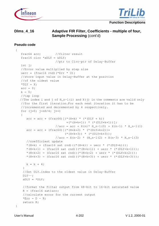
Function Descriptions
Pseudo code
{ frac64 acc; //filter result frac16 circ *aDLY = &DLY; //ptr to Circ-ptr of Delay-Buffer int j; //Error value multiplied by step size uerr = (frac16 rnd)(*Err * U); //store input value in Delay-Buffer at the position //of the oldest value *DLY = X; acc = 0; k = 0; //tap loop //The index i and j of H_n-1(i) and X(j) in the comments are valid only //for the first iteration.For each next iteration it has to be //incremented and decremented by 4 respectively. for (j=0; j<nH/4; j++) { acc = acc + (frac64)[(*(H+k) * (*(DLY + k)) +(*(H+k+1)) * (*(DLY+k+1))]; //acc = acc + X(n)* H_n-1(0) + X(n-1) * H_n-1(1) acc = acc + (frac64)[(*(H+k+2) * (*(DLY+k+2))+ (*(H+k+3)) * (*(DLY+k+3)); //acc = X(n-2) * (H_n-1(2) + X(n-3) * H_n-1(3) //coefficient update *(H+k) = (frac16 sat rnd)((*(H+k)) + uerr * (*(DLY+k))); *(H+k+1) = (frac16 sat rnd)((*(H+k+1)) + uerr * (*(DLY+k+1))); *(H+k+2) = (frac16 sat rnd))(*(H+k+2) + uerr * (*(DLY+k+2))); *(H+k+3) = (frac16 sat rnd)((*(H+k+3)) + uerr * (*(DLY+k+3))); k = k + 4; } //Set DLY.index to the oldest value in Delay-Buffer DLY--; aDLY = *DLY;
//format the filter output from 48-bit to 16-bit saturated value R = (frac16 sat)acc; //calculate error for the current output *Err = D - R; return R;}
Dlms_4_16 Adaptive FIR Filter, Coefficients - multiple of four, Sample Processing (cont’d)
User’s Manual 4-202 V 1.2, 2000-01

Function Descriptions
Techniques • Loop unrolling, four taps/loop • Use of packed data Load/Store• Delay line implemented as circular-buffer • Use of dual MAC instructions• Intermediate result stored in 64-bit register (16 guard bits)• Instruction ordering for zero overhead Load/Store
Assumptions • Filter size must be multiple of four• Inputs, outputs, coefficients are in 1Q15 format• Delay-Buffer is in Internal Memory
Memory Note
Figure 4-49 Dlms_4_16
Dlms_4_16 Adaptive FIR Filter, Coefficients - multiple of four, Sample Processing (cont’d)
Delay-Buffer
aDLYcaDLY.
x(n-nH+1)
x(n)
x(n-1)
x(n-2)
.
.
.
1Q15
doublewordaligned
Hn-1(1)
.
.
.
.
.
Hn-1(0)
Hn-1(nH-1)
1Q15
DualMAC
aH
Coeff-BufferX
(Must be in IntMem)
User’s Manual 4-203 V 1.2, 2000-01

Function Descriptions
Figure 4-50 Dlms_4_16 Coefficient update
Dlms_4_16 Adaptive FIR Filter, Coefficients - multiple of four, Sample Processing (cont’d)
Delay-Buffer
aDLYcaDLY.
x(n-nH+1)
x(n)
x(n-1)
x(n-2)
.
.
.
1Q15
doublewordaligned
Error Value
Dual Mac
CoefficientUpdate
Hn(1)
.
.
.
.
.
Hn(0)
Hn(nH-1)
1Q15
UpdatedCoefficient
Errn = D - R
Errn-1
aH
User’s Manual 4-204 V 1.2, 2000-01

Function Descriptions
Implementation LMS algorithm has been used to realize an adaptive FIR filter. The implemented filter is a Delayed LMS adaptive filter. That is, the updation of coefficients in the current instant is done using the error in the previous output.
The FIR filter is implemented using transversal structure and is realized as a tapped delay line.
This routine processes one sample at a time and returns output of that sample. The input for which the output is to be calculated is sent as an argument to the function.
TriCore’s load doubleword instruction loads four delay line values and four coefficients in one cycle. Dual MAC instruction performs a pair of multiplications and additions according to the equation
[4.73]
where, k=0,1,...., nH-1.
The coefficient is updated using error from the previousoutput, i.e., errn-1. As Hn-1(0) and Hn-1(1) are packed in oneregister, one dual MAC instruction can be used to update boththe coefficients in one cycle. TriCore provides a dual MACinstruction which performs packed multiplication and additionwith rounding and saturation. Hence the two coefficients areupdated at a time and packed in one register according to theequation
[4.74]
where, k=0,1,...,nH-1.
Dlms_4_16 Adaptive FIR Filter, Coefficients - multiple of four, Sample Processing (cont’d)
acc acc X n k–( ) Hn 1– k( ) X n k 1–( )–( )Hn 1– k 1+( )⋅
+⋅+=
Hn k( ) Hn 1– k( ) X n k–( ) Errn 1–⋅+=
Hn k 1+( ) Hn 1– k 1+( ) X n k 1–( )–( ) Errn 1–⋅+=
User’s Manual 4-205 V 1.2, 2000-01

Function Descriptions
Thus by using four dual MAC operations, four coefficients areused and updated on a single pass through the loop. Thisbrings down the loop count by a factor of four. For the sake ofoptimization one set of four dual MACs are performed outsidethe loop. Hence loop is unrolled. This implies it is executed(nH/4-1) times. For delay line, circular addressing mode isused which helps in efficient delay update. The size of thecircular delay buffer is equal to the filter order, i.e., the numberof coefficients. Circular buffer needs doubleword alignmentand to use load doubleword instruction, size of the buffershould be multiple of eight bytes. This implies that thecoefficients should be multiple of four.
Note: To use load doubleword instruction for delay line, thedelay-buffer should be in internal memory only.
Example Trilib\Example\Tasking\Filters\Adaptive\expDlms_4_16.c, expDlms_4_16.cppTrilib\Example\GreenHills\Filters\Adaptive\expDlms_4_16.cpp, expDlms_4_16.cTrilib\Example\GNU\Filters\Adaptive\expDlms_4_16.c
Cycle Count With DSP Extensions
Pre-kernel : 12
Kernel :
if TapLoopCount > 1
if TapLoopCount = 1
Post-kernel : 4+2
Dlms_4_16 Adaptive FIR Filter, Coefficients - multiple of four, Sample Processing (cont’d)
nH4
------- 1– 4 2+×
nH4
------- 1– 4 1+×
User’s Manual 4-206 V 1.2, 2000-01

Function Descriptions
Without DSP Extensions
Pre-kernel : 12
Kernel : same as With DSP Extensions
Post-kernel : 5+2
Code Size 130 bytes
Dlms_4_16 Adaptive FIR Filter, Coefficients - multiple of four, Sample Processing (cont’d)
User’s Manual 4-207 V 1.2, 2000-01

Function Descriptions
DlmsBlk_4_16 Adaptive FIR Filter, Coefficients - multiple of four, Block Processing
Signature void DlmsBlk_4_16(DataS *X, DataS *R, cptrDataS H, cptrDataS *DLY, int nX, DataS *D, DataS *Err, DataS U );
Inputs X : Pointer to Input-Buffer
R : Pointer to Output-Buffer
H : With DSP Extension - circular pointer of Coeff-Buffer of size nHWithout DSP Extension - circ-Struct. Whose members are base address, size and index
DLY : With DSP Extension - Pointer to circular pointer of Delay-Buffer of size nH, where nH is the filter orderWithout DSP Extension - Pointer to Circ-Struct
D : Pointer to Desired-Output-Buffer
Err : Pointer to Error value
U : Step size
Output DLY : Updated circular pointer with index set to the oldest value of the filter Delay-Buffer
H(nH) : Modified Coeff-Buffer
R(nX) : Output-Buffer
Return None
Description Delayed LMS algorithm implemented for adaptive FIR filter, FIR filter transversal structure (direct form), Block processing, 16-bit fractional input, coefficients and output data format, Optimal implementation, requires filter order to be multiple of four.
User’s Manual 4-208 V 1.2, 2000-01

Function Descriptions
Pseudo code
{ frac64 acc; //filter result frac16 circ *aDLY = &DLY; //ptr to Circ-ptr of Delay-Buffer int i, j; //loop for input buffer for (i=0; i<nX; i++) { //Error value multiplied by step size uerr = (frac16 rnd)(*Err * U); //store input value in Delay-Buffer at the position //of the oldest value *DLY = *X++; acc = 0; k = 0; //tap loop for (j=0; j<nH/4; j++) { acc = acc + (frac64)[(*(H+k) * (*(DLY + k)) +(*(H+k+1)) * (*(DLY+k+1))]; //acc = acc + X(n)* H_n-1(0) + X(n-1) * H_n-1(1) acc = acc + (frac64)[(*(H+k+2) * (*(DLY+k+2))+ (*(H+k+3)) * (*(DLY+k+3)); //acc = X(n-2) * (H_n-1(2) + X(n-3) * H_n-1(3) //coefficient update *(H+k) = (frac16 sat rnd)((*(H+k)) + uerr * (*(DLY+k))); *(H+k+1) = (frac16 sat rnd)((*(H+k+1)) + uerr * (*(DLY+k+1))); *(H+k+2) = (frac16 sat rnd))(*(H+k+2) + uerr * (*(DLY+k+2))); *(H+k+3) = (frac16 sat rnd)((*(H+k+3)) + uerr * (*(DLY+k+3))); k = k + 4; } //Set DLY.index to the oldest value in Delay-Buffer DLY--; aDLY = *DLY; //format the filter output from 48-bit to 16-bit saturated value //and store to Output-Buffer *R = (frac16 sat)acc; //calculate error for the current output *Err = *D++ - *R++; }}
DlmsBlk_4_16 Adaptive FIR Filter, Coefficients - multiple of four, Block Processing (cont’d)
User’s Manual 4-209 V 1.2, 2000-01

Function Descriptions
Techniques • Loop unrolling, four taps/loop • Use of packed data Load/Store• Delay line implemented as circular-buffer • Use of dual MAC instructions• Intermediate result stored in 64-bit register (16 guard bits)• Instruction ordering for zero overhead Load/Store
Assumptions • Filter size is a multiple of four• Inputs, outputs, coefficients are in 1Q15 format• Delay-Buffer is in internal memory
Memory Note
Figure 4-51 DlmsBlk_4_16
DlmsBlk_4_16 Adaptive FIR Filter, Coefficients - multiple of four, Block Processing (cont’d)
Input-Buffer Delay-Buffer
aX
aDLYcaDLY.
x(n-nH+1)
x(n)
x(n-1)
x(n-2)
.
.
.
1Q15
doublewordaligned
Hn-1(1)
.
.
.
.
.
Hn-1(0)
Hn-1(nH-1)
1Q15
doublewordaligned
DualMAC
X(1)
.
.
.
X(n)
.
X(0)
.
aH
Coeff-Buffer
halfwordaligned
1Q15
caH
(Must be in IntMem)
User’s Manual 4-210 V 1.2, 2000-01

Function Descriptions
Figure 4-52 DlmsBlk_4_16 Coefficient update
DlmsBlk_4_16 Adaptive FIR Filter, Coefficients - multiple of four, Block Processing (cont’d)
Delay-Buffer
aDLYcaDLY.
x(n-nH+1)
x(n)
x(n-1)
x(n-2)
.
.
.
1Q15
doublewordaligned
Desired OutputBuffer
1Q15
aD
D(1)
.
.
.
.
D(n)
D(0)
.
Output-Buffer
1Q15
aR
R(1)
.
.
.
.
R(n)
R(0)
.
Error Value
Dual Mac
CoefficientUpdate
Hn(1)
.
.
.
.
.
Hn(0)
Hn(nH-1)
1Q15
doublewordaligned
UpdatedCoefficient
Errn = D(n) - R(n)
Errn-1
aH
User’s Manual 4-211 V 1.2, 2000-01

Function Descriptions
Implementation This DLMS routine processes a block of input values at a time. The pointer to the input buffer is sent as an argument to the function. The output is stored in output buffer, the starting address of which is also sent as an argument to the function.
Implementation details are same as Dlms_4_16, except that the Coeff-Buffer is also circular and needs doubleword alignment. The advantage of using circular buffer for coefficients is efficient pointer update. In this implementation while exiting the tap loop, the first two coefficients are already loaded for the next input value. This helps in saving one cycle in the next sample processing.
Example Trilib\Example\Tasking\Filters\Adaptive\expDlmsBlk_4_16.c, expDlmsBlk_4_16.cppTrilib\Example\GreenHills\Filters\Adaptive\expDlmsBlk_4_16.cpp, expDlmsBlk_4_16.cTrilib\Example\GNU\Filters\Adaptive\expDlmsBlk_4_16.c
Cycle Count With DSP Extensions
Pre-loop : 7
Loop :
Post-loop : 1+2
Without DSP Extensions
Pre-loop : 8
Loop : same as With DSP Extensions
DlmsBlk_4_16 Adaptive FIR Filter, Coefficients - multiple of four, Block Processing (cont’d)
nX 8nH4
------- 1– 4 6+×+
×
+1+2
User’s Manual 4-212 V 1.2, 2000-01

Function Descriptions
Post-loop : 1+2
Code Size 166 bytes
DlmsBlk_4_16 Adaptive FIR Filter, Coefficients - multiple of four, Block Processing (cont’d)
User’s Manual 4-213 V 1.2, 2000-01
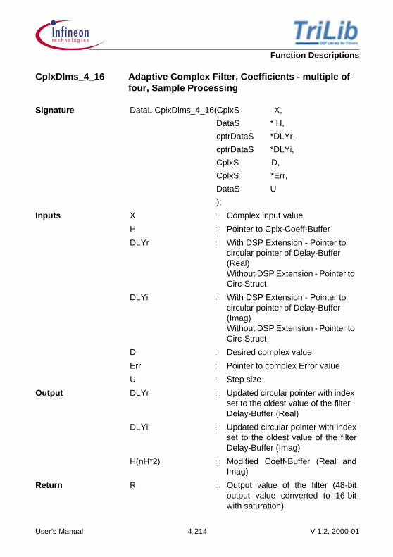
Function Descriptions
CplxDlms_4_16 Adaptive Complex Filter, Coefficients - multiple of four, Sample Processing
Signature DataL CplxDlms_4_16(CplxS X,
DataS * H,
cptrDataS *DLYr,
cptrDataS *DLYi,
CplxS D,
CplxS *Err,
DataS U
);
Inputs X : Complex input value
H : Pointer to Cplx-Coeff-Buffer
DLYr : With DSP Extension - Pointer to circular pointer of Delay-Buffer (Real)Without DSP Extension - Pointer to Circ-Struct
DLYi : With DSP Extension - Pointer to circular pointer of Delay-Buffer (Imag)Without DSP Extension - Pointer to Circ-Struct
D : Desired complex value
Err : Pointer to complex Error value
U : Step size
Output DLYr : Updated circular pointer with index set to the oldest value of the filter Delay-Buffer (Real)
DLYi : Updated circular pointer with indexset to the oldest value of the filterDelay-Buffer (Imag)
H(nH*2) : Modified Coeff-Buffer (Real andImag)
Return R : Output value of the filter (48-bitoutput value converted to 16-bitwith saturation)
User’s Manual 4-214 V 1.2, 2000-01

Function Descriptions
Description Delayed LMS algorithm implemented for adaptive Complex FIR filter, FIR filter transversal structure (direct form), Single sample processing, 16-bit fractional input, coefficients and output data format, Optimal implementation, requires filter order to be multiple of four.
Pseudo code
{ frac64 accr,acci; //Filter result int i,j,k; frac16circ *aDLYr=&DLYr, *aDLYi=&DLYi; //Ptr to circ-ptr of real and imaginary Delay-Buffer //Error value multiplied by step size uerrr = (frac16 rnd)(*Errr * U); uerri = (frac16 rnd)(*Erri * U);
//Store input value in Delay-Buffer at the position of the //oldest value *DLYi = Xi //Imag part of Input is stored in delay line(imag) *DLYr = Xr //Real part of Input is stored in delay line(real)
accr = 0.0; acci = 0.0;
k=0; //tap loop for(j=0; j<nH/2; j++) { //Filter result //Imag acci += (frac64)(*(H+k) * (*(DLYi+k)) + (*(H+k+1) * (*(DLYi+k+1))); //acci += Xi(n) * Hr_n-1(0) + Xi(n-1) * Hr_n-1(1) acci -= (frac64)(*(H+k+2) * (*(DLYr+k)) + (*(H+k+3) * (*(DLYr+k+1))); //acci += Xr(n) * Hi_n-1(0) + Xr(n-1) * Hi_n-1(1) //Real accr += (frac64)(*(H+k) * (*(DLYr+k)) + (*(H+k+1) * (*(DLYr+k+1))); //accr += Xr(n) * Hr_n-1(0) + Xr(n-1) * Hr_n-1(1) accr -= (frac64)(*(H+k+2) *(*(DLYi+k)) + (*(H+k+3) * (*(DLYi+k+1))); //accr -= Xi(n) * Hi_n-1(0) + Xi(n-1) * Hi_n-1(1)
CplxDlms_4_16 Adaptive Complex Filter, Coefficients - multiple of four, Sample Processing (cont’d)
User’s Manual 4-215 V 1.2, 2000-01

Function Descriptions
//Coefficient update //Real_i *(H+k) = (frac16 sat rnd)(*(H+k) + (uerrr * (*(DLYr+k))); //Hr_n(0) = Hr_n-1(0) + Xr(n) * Errr_n-1 *(H+k) = (frac16 sat rnd)(*(H+k) - (uerri * (*(DLYi+k))); //Hr_n(0) -= Xi(n) * Erri_n-1 //Real_i+1 *(H+k+1) = (frac16 sat rnd)(*(H+k+1) + (uerrr * (*DLYr+k+1))); //Hr_n(1) = Hr_n-1(1) + Xr(n-1) * Errr_n-1 *(H+k+1) = (frac16 sat rnd)(*(H+k+1) - (uerri * (*(DLYi+k+1))); //Hr_n(1) -= Xi(n-1) * Erri_n-1
//Imag_i *(H+k+2) = (frac16 sat rnd)(*(H+k+2) + (uerri * (*(DLYr+k))); //Hi_n(0) = Hi_n-1(0) + Xr(n) * Erri_n-1 *(H+k+2) = (frac16 sat rnd)(*(H+k+2) + (uerrr * (*(DLYi+k))); //Hi_n(0) += Xi(n) * Errr_n-1 //Imag_i+1 *(H+k+3) = (frac16 sat rnd)(*(H+k+3) + (uerri * (*(DLYr+k+1))); //Hi_n(1) = Hi_n-1(1) + Xr(n-1) * Erri_n-1 *(H+k+3) = (frac16 sat rnd)(*(H+k+3) + (uerrr * (*(DLYi+k+1))); //Hi_n(1) += Xi(n-1) * Errr_n-1
k=k+4; }
//Set DLYr.index and DLYi.index to the oldest value in Delay-Buffer *DLYr--; *DLYi--; aDLYr = &DLYr; aDLYi = &DLYi;
//Format the real and imaginary parts of the filter output from //48-bit to 16-bit saturated values and pack them in the return //register (Rr : Ri) RLo = (frac16 sat)acci; RHi = (frac16 sat)accr;
//Calculate error in current output *Err = D - R; }}
CplxDlms_4_16 Adaptive Complex Filter, Coefficients - multiple of four, Sample Processing (cont’d)
User’s Manual 4-216 V 1.2, 2000-01

Function Descriptions
Techniques • Loop unrolling, four taps/loop• Use of packed data Load/Store• Delay line implemented as circular-buffer• Use of dual MAC instructions• Intermediate result stored in 64-bit register (16 guard bits)• Instruction ordering for zero overhead Load/Store
Assumptions • Filter size is a multiple of four• Inputs, outputs, coefficients are in 1Q15 format
CplxDlms_4_16 Adaptive Complex Filter, Coefficients - multiple of four, Sample Processing (cont’d)
User’s Manual 4-217 V 1.2, 2000-01

Function Descriptions
Memory Note
Figure 4-53 CplxDlms_4_16
CplxDlms_4_16 Adaptive Complex Filter, Coefficients - multiple of four, Sample Processing (cont’d)
Delay-Buffer(Real)
aDLYrcaDLYr
.
Xr(n-nH+1)
Xr(n)
Xr(n-1)
Xr(n-2)
.
.
.
DualMAC
Real 1
1Q15
doublewordaligned
aDLYi caDLYi
.
Xi(n-nH+1)
Xi(n)
Xi(n-1)
Xi(n-2)
.
.
.
1Q15
doublewordaligned
Hrn-1(1)
Hin-1(0)
Hin-1(1)
.
.
Hin-1(H-2)
Hrn-1(0)
Hin-1(H-1)
1Q15
DualMAC
Real 2
DualMAC
Imag 1
DualMAC
Imag 2
Delay-Buffer(Imag)
Xr Xi
User’s Manual 4-218 V 1.2, 2000-01

Function Descriptions
Figure 4-54 CplxDlms_4_16
CplxDlms_4_16 Adaptive Complex Filter, Coefficients - multiple of four, Sample Processing (cont’d)
Delay-Buffer(Real)
aDLYrcaDLYr.
Xr(n-nH+1)
Xr(n)
Xr(n-1)
Xr(n-2)
.
.
.
1Q15
doublewordaligned
aDLYi caDLYi.
Xi(n-nH+1)
Xi(n)
Xi(n-1)
Xi(n-2)
.
.
.
1Q15
doublewordaligned
Delay-Buffer(Imag)
Errin-1
Errrn-1
Complex ErrorValue
Dual MacReal
Dual MacImag
Dual MacReal
Dual MacImag
CoefficientUpdate
Hrn(1)
Hin(0)
Hin(1)
.
.
Hin(nH-2)
Hrn(0)
Hin(nH-1)
1Q15halfwordaligned
Updated Coeff-Buffer
aHErrrn = Dr - Rr
Errin = Di - Ri
User’s Manual 4-219 V 1.2, 2000-01

Function Descriptions
Implementation Delayed LMS has been implemented for realizing an adaptive complex FIR filter. Circular addressing mode is used for Delay-Buffer. As the filter is complex, two delay buffers are initialized, one for real part of input and the other for imaginary part of the input. The real and imaginary part of the input are separated and they replace the oldest value in the corresponding delay buffers.
To make use of the dual MAC feature of TriCore, coefficients are arranged in a special way as shown in the memory note. Real parts of a pair of coefficients are packed in a register using load word instruction. The corresponding imaginary parts are packed into another register.
A pair of real part of input and a pair of imaginary part of input are also packed in two registers in one cycle each by using the load word instruction.
The complex multiplication requires four multiplications (real -real, imaginary - imaginary, real - imaginary and imaginary-real). Four dual MACs are used which perform each of the above multiplications for a pair of inputs at a time and accumulate the result separately for real and imaginary parts. Hence the loop is executed nH/2 times. Similarly coefficient updation requires four more dual MACs with rounding and saturation. Loop unrolling is done for efficient update of delay line. Thus tap loop is executed (nH/2-1) times. The accumulated real and imaginary parts of the result are formatted to 16-bit saturated value and packed into the return register.
Example Trilib\Example\Tasking\Filters\Adaptive\expCplxDlms_4_16.c, expCplxDlms_4_16.cppTrilib\Example\GreenHills\Filters\Adaptive\expCplxDlms_4_16.cpp, expCplxDlms_4_16.cTrilib\Example\GNU\Filters\Adaptive\expCplxDlms_4_16.c
CplxDlms_4_16 Adaptive Complex Filter, Coefficients - multiple of four, Sample Processing (cont’d)
User’s Manual 4-220 V 1.2, 2000-01

Function Descriptions
Cycle Count With DSP Extensions
Pre-kernel : 14
Kernel :
Post-kernel : 13+2
Without DSP Extensions
Pre-kernel : 3
Kernel : same as With DSP Extensions
Post-kernel : 13+2
Code Size 206 bytes
CplxDlms_4_16 Adaptive Complex Filter, Coefficients - multiple of four, Sample Processing (cont’d)
8nH2
------- 1– 1+× 1+
User’s Manual 4-221 V 1.2, 2000-01

Function Descriptions
CplxDlmsBlk_4_16 Adaptive Complex Filter, Coefficients - multiple of four, Block Processing
Signature void CplxDlmsBlk_4_16(CplxS *X, CplxS *R, DataS *H, cptrDataS *DLYr, cptrDataS *DLYi, int nX, CplxS *D, CplxS *Err, DataS U );
Inputs X : Pointer to complex Input-Buffer
R : Pointer to complex Output-Buffer
H : Pointer to Cplx-Coeff-Buffer
DLYr : With DSP Extension - Pointer to circular pointer of Delay-Buffer (Real)Without DSP Extension - Pointer to Circ-Struct
DLYi : With DSP Extension - Pointer to circular pointer of Delay-Buffer (Imag)Without DSP Extension - Pointer to Circ-Struct
nX : Size of complex Input-Buffer
D : Pointer to complex Desired-Output-Buffer
Err : Pointer to complex Error value
U : Step size
Output DLYr : Updated circular pointer with index set to the oldest value of the filter Delay-Buffer (Real)
DLYi : Updated circular pointer with index set to the oldest value of the filter Delay-Buffer (Imag)
User’s Manual 4-222 V 1.2, 2000-01

Function Descriptions
H(nH*2) : Modified Coeff-Buffer (Real and Imag)
R(nX) : Complex Output-Buffer
Return None
Description Delayed LMS algorithm implemented for adaptive Complex FIR filter, FIR filter transversal structure (direct form), Block processing, 16-bit fractional input, coefficients and output data format, Optimal implementation, requires filter order to be multiple of four.
Pseudo code
{ frac64 accr,acci; //Filter result int i,j,k; frac16circ *aDLYr=&DLYr, *aDLYi=&DLYi; //Ptr to circ-ptr of real and imaginary Delay-Buffer for(i=0; i<nX; i++) { //Error value multiplied by step size uerrr = (frac16 rnd)(*Errr * U); uerri = (frac16 rnd)(*Erri * U);
//Store input value in Delay-Buffer at the position of the //oldest value *DLYi = *X++;//Imag part of Input *DLYr = *X++;//Real part of Input
accr = 0.0; acci = 0.0;
k=0; //tap loop
CplxDlmsBlk_4_16 Adaptive Complex Filter, Coefficients - multiple of four, Block Processing (cont’d)
User’s Manual 4-223 V 1.2, 2000-01

Function Descriptions
for(j=0; j<nH/2; j++) { //Filter result //Imag acci += (frac64)(*(H+k) * (*(DLYi+k)) + (*(H+k+1) * (*(DLYi+k+1))); //acci += Xi(n) * Hr_n-1(0) + Xi(n-1) * Hr_n-1(1) acci -= (frac64)(*(H+k+2) * (*(DLYr+k)) + (*(H+k+3) * (*(DLYr+k+1))); //acci += Xr(n) * Hi_n-1(0) + Xr(n-1) * Hi_n-1(1) //Real accr += (frac64)(*(H+k) * (*(DLYr+k)) + (*(H+k+1) * (*(DLYr+k+1))); //accr += Xr(n) * Hr_n-1(0) + Xr(n-1) * Hr_n-1(1) accr -= (frac64)(*(H+k+2) * (*(DLYi+k)) + (*(H+k+3) * (*(DLYi+k+1))); //accr -= Xi(n) * Hi_n-1(0) + Xi(n-1) * Hi_n-1(1) //Coefficient update //Real_i *(H+k) = (frac16 sat rnd)(*(H+k) + (uerrr * (*(DLYr+k))); //Hr_n(0) = Hr_n-1(0) + Xr(n) * Errr_n-1 *(H+k) = (frac16 sat rnd)(*(H+k) - (uerri * (*(DLYi+k))); //Hr_n(0) -= Xi(n) * Erri_n-1 //Real_i+1 *(H+k+1) = (frac16 sat rnd)(*(H+k+1) + (uerrr * (*DLYr+k+1))); //Hr_n(1) = Hr_n-1(1) + Xr(n-1) * Errr_n-1 *(H+k+1) = (frac16 sat rnd)(*(H+k+1) - (uerri * (*(DLYi+k+1))); //Hr_n(1) -= Xi(n-1) * Erri_n-1
//Imag_i *(H+k+2) = (frac16 sat rnd)(*(H+k+2) + (uerri * (*(DLYr+k))); //Hi_n(0) = Hi_n-1(0) + Xr(n) * Erri_n-1 *(H+k+2) = (frac16 sat rnd)(*(H+k+2) + (uerrr * (*(DLYi+k))); //Hi_n(0) += Xi(n) * Errr_n-1 //Imag_i+1 *(H+k+3) = (frac16 sat rnd)(*(H+k+3) + (uerri * (*(DLYr+k+1))); //Hi_n(1) = Hi_n-1(1) + Xr(n-1) * Erri_n-1 *(H+k+3) = (frac16 sat rnd)(*(H+k+3) + (uerrr * (*(DLYi+k+1))); //Hi_n(1) += Xi(n-1) * Errr_n-1
k=k+4; }
CplxDlmsBlk_4_16 Adaptive Complex Filter, Coefficients - multiple of four, Block Processing (cont’d)
User’s Manual 4-224 V 1.2, 2000-01

Function Descriptions
//Set DLYr.index and DLYi.index to the oldest value in Delay-Buffer *DLYr--; *DLYi--; aDLYr = &DLYr; aDLYi = &DLYi;
//Format the real and imaginary parts of the filter output //from 48 bit to 16-bit saturated values and store the //result to Output-Buffer *RLo = (frac16 sat)acci; *RHi = (frac16 sat)accr; R++; //Calculate error in current output *Err = *D++ - *R++; }//end of indata loop
}//end of main
Techniques • Loop unrolling, two taps/loop • Use of packed data Load/Store• Delay line implemented as circular-buffer• Use of dual MAC instructions• Intermediate result stored in 64-bit register (16 guard bits)• Instruction ordering for zero overhead Load/Store
Assumptions • Filter size is a multiple of four• Inputs, outputs, coefficients are in 1Q15 format
CplxDlmsBlk_4_16 Adaptive Complex Filter, Coefficients - multiple of four, Block Processing (cont’d)
User’s Manual 4-225 V 1.2, 2000-01
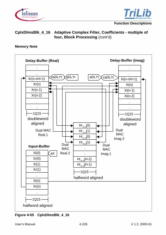
Function Descriptions
Memory Note
Figure 4-55 CplxDlmsBlk_4_16
CplxDlmsBlk_4_16 Adaptive Complex Filter, Coefficients - multiple of four, Block Processing (cont’d)
Input-Buffer
Delay-Buffer (Real)
aX
aDLYrcaDLYr.
Xr(n-nH+1)
Xr(n)
Xr(n-1)
Xr(n-2)
.
.
.
Dual MACReal 1
1Q15
1Q15
doublewordaligned
aDLYi caDLYi.
Xi(n-nH+1)
Xi(n)
Xi(n-1)
Xi(n-2)
.
.
.
1Q15
doublewordaligned
Hrn-1(1)
Hi n-1(0)
Hi n-1(1)
.
.
Hin-1(H-2)
Hrn-1(0)
Hin-1(H-1)
1Q15
halfword aligned
DualMAC
Real 2
DualMAC
Imag 1
DualMAC
Imag 2
Delay-Buffer (Imag)
Xr(0)
Xi(1)
Xr(1)
.
Xi(n)
Xr(n)
Xi(0)
.
halfword aligned
User’s Manual 4-226 V 1.2, 2000-01

Function Descriptions
Figure 4-56 CplxDlmsBlk_4_16 Coefficient update
CplxDlmsBlk_4_16 Adaptive Complex Filter, Coefficients - multiple of four, Block Processing (cont’d)
Delay-Buffer (Real)
aDLYrcaDLYr.
Xr(n-nH+1)
Xr(n)
Xr(n-1)
Xr(n-2)
.
.
.
1Q15
doublewordaligned
aDLYi caDLYi.
Xi(n-nH+1)
Xi(n)
Xi(n-1)
Xi(n-2)
.
.
.
1Q15doubleword
aligned
Delay-Buffer (Imag)
DesiredOutput Buffer
1Q15
aR
Dr(0)
Di(1)
Dr(1)
.
Di(n)
Dr(n)
Di(0)
.
Errin-1
Errrn-1
Output-Buffer
aR
Rr(0)
Ri(1)
Rr(1)
.
Ri(n)
Rr(n)
Ri(0)
.
Complex ErrorValue
Dual Mac Real Dual Mac Imag
Dual MacReal
Dual MacImag
CoefficientUpdate
Hrn(1)
Hin(0)
Hin(1)
.
.
Hin(nH-2)
Hrn(0)
Hin(nH-1)
1Q15halfwordaligned
UpdatedCoeff- Buffer
Errrn = Dr(n) - Rr(n)
Errin = Di(n) - Ri(n)
1Q15
aH
halfwordaligned
halfwordaligned
User’s Manual 4-227 V 1.2, 2000-01

Function Descriptions
Implementation This DLMS routine processes a block of input values at a time. The pointer to the input buffer is sent as an argument to the function. The output is stored in output buffer, the starting address of which is also sent as an argument to the function.
Implementation details are same as CplxDlms_4_16. An additional loop is needed to calculate the output for every sample in the buffer. Hence, this loop is repeated as many times as the size of the input buffer.
Example Trilib\Example\Tasking\Filters\Adaptive\expCplxDlmsBlk_4_16.c, expCplxDlmsBlk_4_16.cppTrilib\Example\GreenHills\Filters\Adaptive\expCplxDlmsBlk_4_16.cpp, expCplxDlmsBlk_4_16.cTrilib\Example\GNU\Filters\Adaptive\expCplxDlmsBlk_4_16.c
Cycle Count With DSP Extensions
Pre-loop : 9
Loop :
Post-loop : 3+2
Without DSP Extensions
Pre-loop : 9
Loop : same as With DSP Extensions
Post-loop : 3+2
Code Size 252 bytes
CplxDlmsBlk_4_16 Adaptive Complex Filter, Coefficients - multiple of four, Block Processing (cont’d)
nX 8nH2
------- 1– 8 16+×+
×
+1+2
User’s Manual 4-228 V 1.2, 2000-01

Function Descriptions
Dlms_2_16x32 Mixed Adaptive FIR Filter, Coefficients - multiple of two, Sample Processing
Signature DataL Dlms_2_16x32(DataS X, DataL *H, cptrDataS *DLY, DataL D, DataL *Err, DataL U );
Inputs X : Real Input Value
H : Pointer to Coeff-Buffer
DLY : With DSP Extension - Pointer to circular pointer of Delay-Buffer of size nH, where nH is the filter orderWithout DSP Extension - Pointer to Circ-Struct
(nH) : Implicit filter order stored in Circ-Ptr DLY
D : Real expected value
Err : Pointer to Error value
U : Step size
Outputs DLY : Updated circular pointer with index set to the oldest value of the filter Delay-Buffer
H(nH) : Modified Coeff-Buffer
Return R : Output value of the filter (32-bitoutput)
Description Delayed LMS algorithm implemented for mixed adaptive FIR filter, FIR filter transversal structure (direct form), Single sample processing, 16-bit fractional input, 32-bit coefficients and output data format, Optimal implementation, requires filter order to be multiple of two.
User’s Manual 4-229 V 1.2, 2000-01

Function Descriptions
Pseudo code
{ frac32 acc; //filter result frac16 circ *aDLY = &DLY; //ptr to Circ-ptr of Delay-Buffer int j; //Error value multiplied by step size uerr = (frac32)(*Err * U); //store input value in Delay-Buffer at the position //of the oldest value *DLY = X; acc = 0; k = 0; //tap loop //The index i and j of H_n-1(i) and X(j) in the comments are valid only //for the first iteration.For each next iteration it has to be //incremented and decremented by 2 respectively. for (j=0; j<nH/2; j++) { acc = acc + (frac32 sat)(*(H+k) * (*(DLY + k))); //acc = acc + X(n)* H_n-1(0) acc = acc + (frac32 sat)(*(H+k+1) * (*(DLY+k+1))); //acc = X(n-1) * (H_n-1(1) //coefficient update *(H+k) = (frac32 sat)((*(H+k)) + uerr * (*(DLY+k))); *(H+k+1) = (frac32 sat)((*(H+k+1)) + uerr * (*(DLY+k+1))); k = k + 2; } //Set DLY.index to the oldest value in Delay-Buffer DLY--; aDLY = *DLY; //filter output stored to output buffer R = acc; //calculate error for the current output *Err = D - R; return R;}
Techniques • Loop unrolling, two taps/loop • Use of packed data Load/Store• Delay line implemented as circular-buffer • Instruction ordering for zero overhead Load/Store
Dlms_2_16x32 Mixed Adaptive FIR Filter, Coefficients - multiple of two, Sample Processing (cont’d)
User’s Manual 4-230 V 1.2, 2000-01

Function Descriptions
Assumptions • Filter order is a multiple of two• Inputs in 1Q15 format, all other parameters in 1Q31 format
Memory Note
Figure 4-57 Dlms_2_16x32
Dlms_2_16x32 Mixed Adaptive FIR Filter, Coefficients - multiple of two, Sample Processing (cont’d)
Delay-Buffer
aDLYcaDLY.
x(n-nH+1)
x(n)
x(n-1)
x(n-2)
.
.
.
1Q15
doublewordaligned
Hn-1(1)
.
.
.
.
.
Hn-1(0)
Hn-1(nH-1)
1Q31
MAC
aH
Coeff-BufferX
User’s Manual 4-231 V 1.2, 2000-01

Function Descriptions
Figure 4-58 Dlms_2_16x32 Coefficient update
Dlms_2_16x32 Mixed Adaptive FIR Filter, Coefficients - multiple of two, Sample Processing (cont’d)
Delay-Buffer
aDLYcaDLY.
x(n-nH+1)
x(n)
x(n-1)
x(n-2)
.
.
.
1Q15
doublewordaligned
Error Value
MAC
CoefficientUpdate
Hn(1)
.
.
.
.
.
Hn(0)
Hn(nH-1)
1Q31
UpdatedCoefficient
Errn = D - R
Errn-1
aH
User’s Manual 4-232 V 1.2, 2000-01

Function Descriptions
Implementation LMS algorithm has been used to realize an adaptive FIR filter. The implemented filter is a Delayed LMS adaptive filter i.e., the updation of coefficients in the current instant is done using the error in the previous output.
The FIR filter is implemented using transversal structure and is realized as a tapped delay line.
This routine processes one sample at a time and returns output of that sample. The input for which the output is to be calculated is sent as an argument to the function.
TriCore’s load word instruction loads two delay line values and two coefficients in one cycle each. MAC instruction performs a multiplication and an addition according to the equation
[4.75]
where, k=0,1,...., nH-1.
The coefficient is updated using error from the previousoutput, i.e., errn-1. A MAC instruction updates a coefficient inone cycle according to the equation
[4.76]
where, k=0,1,...,nH-1.
By using four MACs two coefficients are used and updated inone pass through the loop. The loop is unrolled for efficientpointer update. Hence tap loop is executed (nH/2 - 1) times.
For delay line, circular addressing mode is used. The size ofthe circular delay buffer is equal to the filter order, i.e., thenumber of coefficients. Circular buffer needs doublewordalignment and to use load word instruction, size of the buffershould be multiple of four bytes. This implies that thecoefficients should be multiple of two.
Dlms_2_16x32 Mixed Adaptive FIR Filter, Coefficients - multiple of two, Sample Processing (cont’d)
acc acc X n k–( ) Hn 1– k( )⋅+=
Hn k( ) Hn 1– k( ) X n k–( ) Errn 1–⋅+=
User’s Manual 4-233 V 1.2, 2000-01

Function Descriptions
Example Trilib\Example\Tasking\Filters\Adaptive\expDlms_2_16x32.c, expDlms_2_16x32.cppTrilib\Example\GreenHills\Filters\Adaptive\expDlms_2_16x32.cpp, expDlms_2_16x32.cTrilib\Example\GNU\Filters\Adaptive\expDlms_2_16x32.c
Cycle Count With DSP Extensions
Pre-kernel : 12
Kernel :
if LoopCount > 1
if LoopCount = 1
Post-kernel : 4+2
Without DSP Extensions
Pre-kernel : 12
Kernel : same as With DSP Extensions
Post-kernel : 4+2
Code Size 108 bytes
Dlms_2_16x32 Mixed Adaptive FIR Filter, Coefficients - multiple of two, Sample Processing (cont’d)
nH2
------- 1– 4 2+×
nH2
------- 1– 4 1+×
User’s Manual 4-234 V 1.2, 2000-01

Function Descriptions
DlmsBlk_2_16x32 Mixed Adaptive FIR Filter, Coefficients - multiple of two, Block Processing
Signature void DlmsBlk_2_16x32(DataS *X, DataL *R, cptrDataL H, cptrDataS *DLY, int nX, DataL *D, DataL *Err, DataL U );
Inputs X : Pointer to Input-Buffer
R : Pointer to Output-Buffer
H : With DSP Extension - circular pointer of Coeff-Buffer of size nHWithout DSP Extension - circ-Struct. Whose members are base address, size and index
DLY : With DSP Extension - Pointer to circular pointer of Delay-Buffer of size nH, where nH is the filter orderWithout DSP Extension - Pointer to Circ-Struct
(nH) : Implicit filter order stored in Circ-Pointer DLY
D : Pointer to Desired-Output-Buffer
Err : Pointer to Error value
U : Step size
Output DLY : Updated circular pointer with index set to the oldest value of the filter Delay-Buffer
H(nH) : Modified Coeff-Buffer
R(nX) : Output-Buffer
Return None
User’s Manual 4-235 V 1.2, 2000-01

Function Descriptions
Description Delayed LMS algorithm implemented for mixed adaptive FIR filter, FIR filter transversal structure (direct form), Block processing, 16-bit fractional input, 32-bit coefficients and output data format, Optimal implementation, requires filter order to be multiple of two.
DlmsBlk_2_16x32 Mixed Adaptive FIR Filter, Coefficients - multiple of two, Block Processing (cont’d)
User’s Manual 4-236 V 1.2, 2000-01

Function Descriptions
Pseudo code
{ frac32 acc; //filter result frac16 circ *aDLY = &DLY; //ptr to Circ-ptr of Delay-Buffer int i, j; //loop for input buffer for (i=0; i<nX; i++) { //Error value multiplied by step size uerr = (frac32 rnd)(*Err * U); //store input value in Delay-Buffer at the position //of the oldest value *DLY = *X++; acc = 0; k = 0; //tap loop for (j=0; j<nH/4; j++) { acc = acc + (frac32 sat)(*(H+k) * (*(DLY + k))); //acc = acc + X(n)* H_n-1(0) acc = acc + (frac32 sat)(*(H+k+1) * (*(DLY+k+1))); //acc = X(n-1) * (H_n-1(1)
//coefficient update *(H+k) = (frac32 sat)((*(H+k)) + uerr * (*(DLY+k))); *(H+k+1) = (frac32 sat)((*(H+k+1)) + uerr * (*(DLY+k+1))); k = k + 2; } //Set DLY.index to the oldest value in Delay-Buffer DLY--; aDLY = *DLY; //filter output stored to output buffer *R = acc; //calculate error for the current output *Err = *D++ - *R++; }}
DlmsBlk_2_16x32 Mixed Adaptive FIR Filter, Coefficients - multiple of two, Block Processing (cont’d)
User’s Manual 4-237 V 1.2, 2000-01

Function Descriptions
Techniques • Loop unrolling, two taps/loop • Use of packed data Load/Store• Delay line and coefficient array implemented as circular-
buffer • Instruction ordering for zero overhead Load/Store
Assumptions • Filter size is a multiple of two• Inputs in 1Q15, all other parameters in 1Q31 format
Memory Note
Figure 4-59 DlmsBlk_2_16x32
DlmsBlk_2_16x32 Mixed Adaptive FIR Filter, Coefficients - multiple of two, Block Processing (cont’d)
Input-Buffer Delay-Buffer
aX
aDLYcaDLY.
X(n-nH+1)
X(n)
X(n-1)
X(n-2)
.
.
.
1Q15
doublewordaligned
Hn-1(1)
.
.
.
.
.
Hn-1(0)
Hn-1(nH-1)
1Q31
doublewordaligned
MAC
X(1)
.
.
.
X(n)
.
X(0)
.
aH
Coeff-Buffer
halfwordaligned
1Q15
caH
User’s Manual 4-238 V 1.2, 2000-01
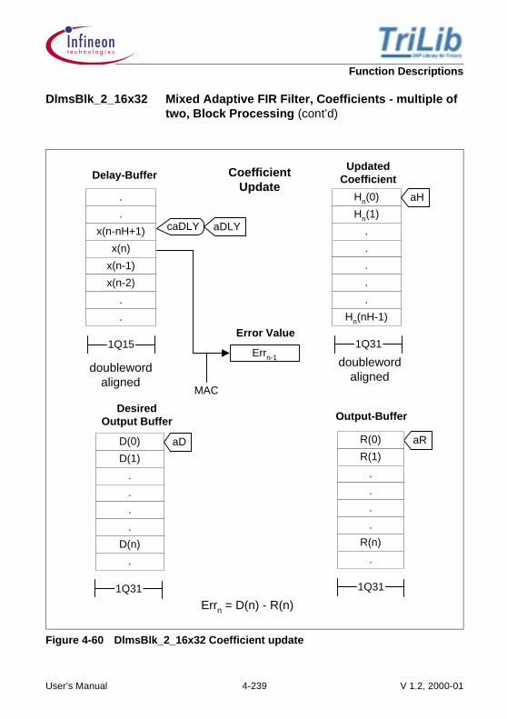
Function Descriptions
Figure 4-60 DlmsBlk_2_16x32 Coefficient update
DlmsBlk_2_16x32 Mixed Adaptive FIR Filter, Coefficients - multiple of two, Block Processing (cont’d)
Delay-Buffer
aDLYcaDLY.
x(n-nH+1)
x(n)
x(n-1)
x(n-2)
.
.
.
1Q15
doublewordaligned
DesiredOutput Buffer
1Q31
aD
D(1)
.
.
.
.
D(n)
D(0)
.
Output-Buffer
1Q31
aR
R(1)
.
.
.
.
R(n)
R(0)
.
Error Value
MAC
CoefficientUpdate
Hn(1)
.
.
.
.
.
Hn(0)
Hn(nH-1)
1Q31
doublewordaligned
UpdatedCoefficient
Errn = D(n) - R(n)
Errn-1
aH
User’s Manual 4-239 V 1.2, 2000-01

Function Descriptions
Implementation This DLMS routine processes a block of input values at a time. The pointer to the input buffer is sent as an argument to the function. The output is stored in output buffer, the starting address of which is also sent as an argument to the function.
Implementation details are same as Dlms_4_16, except that the Coeff-Buffer is also circular and needs doubleword alignment. The advantage of using circular buffer for coefficients is efficient pointer update. In this implementation while exiting the tap loop, the first two coefficients are already loaded for the next input value. This helps in saving one cycle in the next sample processing.
Example Trilib\Example\Tasking\Filters\Adaptive\expDlmsBlk_2_16x32.c, expDlmsBlk_2_16x32.cppTrilib\Example\GreenHills\Filters\Adaptive\expDlmsBlk_2_16x32.cpp, expDlmsBlk_2_16x32.cTrilib\Example\GNU\Filters\Adaptive\expDlmsBlk_2_16x32.c
Cycle Count With DSP Extensions
Pre-loop : 7
Loop (for input data) :
Post-loop : 1+2
Without DSP Extensions
Pre-loop : 8
Loop : same as With DSP Extensions
Post-loop : 1+2
Code Size 136 bytes
DlmsBlk_2_16x32 Mixed Adaptive FIR Filter, Coefficients - multiple of two, Block Processing (cont’d)
nX 9nH2
------- 1– 4 6+×+×
+1+2
User’s Manual 4-240 V 1.2, 2000-01

Function Descriptions
4.7 Fast Fourier Transforms
Spectrum (Spectral) analysis is a very important methodology in Digital SignalProcessing. Many applications have a requirement of spectrum analysis. The spectrumanalysis is a process of determining the correct frequency domain representation of thesequence. The analysis gives rise to the frequency content of the sampled waveformsuch as bandwidth and centre frequency.
One of the method of doing the spectrum analysis in Digital Signal Processing is byemploying the Discrete Fourier Transform (DFT).
The DFT is used to analyze, manipulate and synthesize signals in ways not possible withcontinuous (analog) signal processing. It is a mathematical procedure that helps indetermining the harmonic, frequency content of a discrete signal sequence. DFTs originis from a continuous fourier transform which is given by
[4.77]
where x(t) is continuous time varying signal and X(f) is the fourier transform of the same.
The DFT is given by
[exponential form] [4.78]
where the DFT coefficients used in the DFT Kernel, W, is
[4.79]
[4.80]
X(k) is the kth DFT output component for k=0,1,2,....,N-1
x(n) is the sequence of discrete sample for n=0,1,2,...,N-1
j is imaginary unit
N is the number of samples of the input sequence (and number of frequency points ofDFT output).
X f( ) x t( )e j2πft–td
∞–
∞
∫=
X k( ) x n( )WNnk
n 0=
N 1–
∑=
WN ej2π– N⁄
=
X k( ) x n( ) 2πnk N⁄ )(cos j 2πnk N⁄( )sin–[ ]
n 0=
N 1–
∑=
1–
User’s Manual 4-241 V 1.2, 2000-01

Function Descriptions
While the DFT is used to convert the signal from time domain to frequency domain. Thecomplementary function for DFT is the IDFT, which is used to convert a signal fromfrequency to time domain. The IDFT is given by
[exponential form] [4.81]
[4.82]
Notice the difference between DFT in Equation [4.78] and Equation [4.80], the IDFTKernel is the complex conjugate of the DFT and the output is scaled by N.
WNnk, the Kernel of the DFT and IDFT is called the Twiddle-Factor and is given by,
In exponential form,
for DFT
for IDFT
In rectangular form,
for DFT
for IDFT
While calculating DFT, a complex summation of N complex multiplications is required foreach of N output samples. N2 complex multiplications and N(N-1) complex additionscompute an N-point DFT. The processing time required by large number of calculationlimits the usefulness of DFT. This drawback of DFT is overcome by a more efficient andfast algorithm called Fast Fourier Transform (FFT). The radix-2 FFT computes the DFTin N*log2(N) complex operations instead of N2 complex operations for that of the DFT.(where N is the transform length.)
The FFT has the following preconditions to operate at a faster rate.
• The radix-2 FFT works only on the sequences with lengths that are power of two.• The FFT has a certain amount of overhead that is unavoidable, called bit reversed
ordering. The output is scrambled for the ordered input or the input has to be arrangedin a predefined order to get output properly arranged. This makes the straight DFTbetter suited for short length computation than FFT. The graph shows the algorithmcomplexity of both on a typical processor like pentium.
x n( ) 1N---- X k( )ej2πnk N⁄
k 0=
N 1–
∑=
x n( ) 1N---- X k( ) 2πnk N⁄( )cos j 2πnk N⁄( )sin+[ ]
k 0=
N 1–
∑=
ej– 2πnk N⁄
ej2πnk N⁄
2πnk N⁄( )cos j 2πnk N⁄( )sin–
2πnk N⁄( )cos j 2πnk N⁄( )sin+
User’s Manual 4-242 V 1.2, 2000-01

Function Descriptions
Figure 4-61 Complexity Graph
The Fourier transform plays an important role in a variety of signal processingapplications. Anytime, if it is more comfortable to work with a signal in the frequencydomain than in the original time or space domain, we need to compute Fourier transform.
Given N input samples of a signal x(n) = 0,1,..., (N-1), its Fourier transform is defined by
[4.83]
Since n is an integer, X(f) is periodic with the period 1. Therefore, we only consider X(f)in the basic interval . In digital computation, X(f) is often evaluated at N uniformlyspaced points f = k/N (k=0,1,.....,N-1). This leads to the Discrete Fourier Transform (DFT)
(k=0,1,.....,N-1) [4.84]
with . Direct computation of this length N, DFT takes N2 complexmultiplications and N(N-1) complex additions. FFT is an incredibly efficient algorithm forcomputing DFT. The main idea of FFT is to exploit the periodic and symmetric properties
0.1
0.01
0.001
correlation DFT
FFT
1
10
100
1000
Exe
cutio
n tim
e (s
econ
ds)
8 16 32 64 128 256 512 1024 40962048Number points in DFT
X f( ) x n( )e j2πfn–
n 0=
N 1–
∑=
0 f 1≤ ≤
X k( ) x n( )WNnk
n 0=
N 1–
∑=
WN ej2π– N⁄
=
User’s Manual 4-243 V 1.2, 2000-01

Function Descriptions
of the DFT Kernel . The resulting algorithm depends strongly on the transformlength N. The basic Cooley-Tukey algorithm assumes that N is a power of two. Hence itis called radix-2 algorithm. Depending on how the input samples x(n) and the output dataX(k) are grouped, either a decimation-in-time (DIT) or a decimation-in-frequency (DIF)algorithm is obtained. The technique used by Cooley and Tukey can also be applied toDFTs, where N is a power of r. The resulting algorithms are referred to as radix-r FFT. Itturns out that radix-4, radix-8, and radix-16 are especially interesting. In cases where Ncannot be represented in terms of powers of single number, mixed-radix algorithms mustbe used. For example for 28 point input, since 28 cannot be represented in terms ofpowers of 2 and 4 we use radix-7 and radix-4 FFT to get the frequency spectrum. Thebasic radix-2 decimation-in-frequency FFT algorithm is implemented.
4.7.1 Radix-2 Decimation-In-Time FFT Algorithm
The decimation-in-time (DIT) FFT divides the input (time) sequence into two groups, oneof even samples and the other of odd samples. N/2-point DFTs are performed on thesesub-sequences and their outputs are combined to form the N-point DFT.
First, x(n) the input sequence in the Equation [4.84] is divided into even and odd sub-sequences.
for k=0 to N-1 [4.85]
But,
By substituting the following in Equation [4.85]
x1(n)=x(2n)
x2(n)=x(2n+1)
Equation [4.85] becomes
for k=0 to N-1 [4.86]
WNnk
X k( ) x 2n( )WN2nk
x 2n 1+( )WN2n 1+( )k
n 0=
2---- 1–
∑+
n 0=
2---- 1–
∑=
x 2n( )WN2nk
WNk
x 2n 1+( )WN2nk
n 0
N2---- 1–
∑+
n 0
N2---- 1–
∑=
WN2nk
ej2π–( ) N⁄( )
2nke
j2π–( ) N 2⁄( )⁄( )nk
WN 2⁄nk
===
X k( ) x1 n( )WN 2⁄nk
WNk
x2 n( )WN 2⁄nk
n 0=
N 2 1–⁄
∑+
n 0=
N 2 1–⁄
∑=
Y k( ) WNk
+ Z k( )=
User’s Manual 4-244 V 1.2, 2000-01

Function Descriptions
Equation [4.86] is the radix-2 DIT FFT equation. It consists of two N/2-point DFTs (Y(k)and Z(k)) performed on the subsequences of even and odd samples respectively of theinput sequence, x(n). Multiples of WN, the Twiddle-Factors are the coefficients in the FFTcalculation.
Further,
[4.87]
Equation [4.86] can be expressed in two equations
[4.88]
[4.89]
for k=0 to N/2-1
The complete 8-point DIT FFT is illustrated in figure.
Figure 4-62 8-point DIT FFT
WNk N 2⁄+
ej– 2π N⁄( )
ke
j– 2π N⁄( )N 2⁄
× WNk
–= =
X k( ) Y k( ) WNkZ k( )+=
X k N 2⁄+( ) Y k( ) WNkZ k( )–=
W2
x0
W0
x3
x5
x7
x1
x2
x6
x4 X1
X2
X3
X4
X6
X5
X7
X0
W0
W3
W2
W1
W2
W0
W0
W0
W0
W0
+
-
+
-
+
+
+
+
+
+
-
-
-
-
-
-
-
-
-
-
+
+
+
+
User’s Manual 4-245 V 1.2, 2000-01

Function Descriptions
The complete 8-point DIF FFT is illustrated in figure.
Figure 4-63 8-point DIF FFT
In the diagram, each pair of arrows represents a Butterfly. The whole of FFT is computedby different patterns of Butterflies. These are called groups and stages.
For 8-point FFT the first stage consists of four groups of one Butterfly each, secondconsists of two groups of two butterflies and third stage has one group of four Butterflies.Each Butterfly is represented as in diagram.
Figure 4-64 Radix-2 DIT Butterfly
W0
x3
x5
x7
x1
x2
x6
x0
x4 X1
X2
X3
X4
X6
X5
X7
X0
W2
W0
W2
W0
W2
W1
W3
+
-
-
+
+
+
+
+
+
+
-
-
-
-
-
-
+
+
+
+
-
-
-
-
Dual nodespacing
x0’+jy0’
x1’+jy1’
x0+jy0
x1+jy1W=C+j(-S)
Primarynode
Dualnode
User’s Manual 4-246 V 1.2, 2000-01

Function Descriptions
The output is derived as follows
[4.90]
[4.91]
[4.92]
[4.93]
x0’ x0 C( )x1 S–( )y1–[ ]+=
y0’ y0 C( )y1 S–( )x1+[ ]+=
x1’ x0 C( )x1 S–( )y1–[ ]–=
y1’ y0 C( )y1 S–( )x1+[ ]–=
User’s Manual 4-247 V 1.2, 2000-01

Function Descriptions
4.8 TriCore Implementation Note
4.8.1 Organization of FFT functions
The FFT radix-2 DIT function set consists of the following functions.
• Forward FFT• Inverse FFT• Forward Real FFT• Inverse Real FFT
The above set of functions makes use of macros for efficient computation. The basic bitreversal module, Butterflies and the Spectrum split operations are implemented in formof macros.
The TriLib FFT implementation is one of the most optimal implementation which makesuse of several optimization techniques. Further, it makes use of different optimizationmethods at instruction level. Secondly, it is organized as macros to save time duringfunction calls and also overcome the conditional checks such as shift etc., which perhapsis done during assembling time itself as it is implemented as macros. Thirdly, thealgorithmic optimization, where the first pass or the first stage Butterflies are computedoutside the loop separately. This saves time as the first stage Butterflies need not bemultiplied by Twiddle-Factors.
4.8.2 16 Bit Implementation Modules
The classical FFT takes the input and Twiddle-Factor in the form of 16 bit complexnumber representation as in Figure 4-2. For computational efficiency and to make useof the parallel architecture of TriCore, a more efficient form of complex representation isdevised for internal operations of the FFT. The REAL:IMAG, REAL:IMAG pairs areconverted to REAL:REAL, IMAG:IMAG representation before processing.
Twiddle-Factors for the computation of 16 bit FFT is done by a utility function calledFFT_TF_16().
The main modules of FFTs are:
FFT_2_16() Forward FFT for 16 bit Complex input, radix-2 decimation-in-time implementation
IFFT_2_16() Inverse FFT for 16 bit Complex input, radix-2 decimation-in-time implementation
User’s Manual 4-248 V 1.2, 2000-01

Function Descriptions
4.8.3 16 bit Implementation for Mixed FFT
The mixed 16 bit FFT is the combination of features of 32 bit and 16 bit FFT, while 16 bitis more efficient and 32 bit is more precise. The mixed FFT is a combination of both. Ithas better precision than 16 bit and better speed than 32 bit implementation.
Internally the mixed FFT uses 32 bit representation and the final stage output isconverted to 16 bit precision using ConvertBuf macro.
Twiddle-Factors for the computation of mixed FFT is done by a utility function calledFFT_TF_16x32().
The main modules of Mixed FFTs are:
4.8.4 32 Bit Implementation
The 32 bit implementation follows the straight forward approach in implementation. Thefirst pass (stage) is done outside the stage loop for the optimization purpose like it isdone in the 16 bit implementation. This is done by the Firstpass macro.
FFTReal_2_16() Forward FFT for 16 bit Real sequence input, radix-2 decimation-in-time implementation
IFFTReal_2_16() Inverse Real FFT for 16 bit Complex sequence input, radix-2 decimation-in-time implementation to generate the two real output sequences
FFT_2_16x32() Forward FFT for 16 bit Complex input, radix-2 decimation-in-time implementation. Internal processing will be 32 bits, output will be rounded to 16 bits
IFFT_2_16x32() Inverse FFT for 16 bit Complex input, radix-2 decimation-in-time implementation. Internal processing will be 32 bits, output will be rounded to 16 bits
FFTReal_2_16x32() Forward FFT for 16 bit Real sequence input, radix-2 decimation-in-time implementation. Internal processing will be 32 bits, output will be rounded to 16 bits
IFFTReal_2_16x32() Inverse Real FFT for 16 bit Complex sequence input, radix-2 decimation-in-time implementation to generate the two real output sequences. Internal processing will be 32 bits, output will be rounded to 16 bits
User’s Manual 4-249 V 1.2, 2000-01

Function Descriptions
Subsequent passes (stages) uses the Butterfly2 macro for the forward FFT and theIButterfly2 macro for the inverse FFT. This is same as the 16 bit implementation, exceptthat this doesn’t need the special arrangement of the data.
Twiddle-Factors for FFT and IFFT are complex conjugate of each other, the Twiddle-Factors calculated for FFT are used for IFFT. The Butterfly calculation for IFFT ischanged accordingly.
The Real FFT uses the Complex FFT functionality for computation and the final outputis split to separate the real part from the complex result and is arranged as a real half inand imaginary half like Re[0], Re[1],...,Re[N/2-1], Im[0], Im[1],...,Im[N/2-1] in acontinuous order.
Twiddle-Factors for the computation of FFT is done by a utility function calledFFT_TF_32() as shown in the example.
The input for the 32 bit FFT, IFFT, RFFT, RIFFT are all in 1Q31 packed into a 64 bit dataas shown in the Figure 4-3 the input and the output is in normal order.
The main modules of FFTs are:
4.8.5 Functional Implementation
The main functions tested in Section 4.8.2 has a generic structure. It uses three nestedloops. It computes the first pass outside the nested loops.
First Stage
The First stage is executed outside the nested loops. The advantage of having this hasbeen already discussed in the Section 4.8.1. The First stage makes use of the
FFT_2_32() Forward FFT for 32 bit Complex input, radix-2 decimation-in-time implementation
IFFT_2_32() Inverse FFT for 32 bit Complex input, radix-2 decimation-in-time implementation
FFTReal_2_32() Forward FFT for 32 bit Real sequence input, radix-2 decimation-in-time implementation
IFFTReal_2_32() Inverse Real FFT for 32 bit Complex sequence input, radix-2 decimation-in-time implementation to generate the two real output sequences
User’s Manual 4-250 V 1.2, 2000-01

Function Descriptions
FirstPass macro. The idea to separate the first stage Butterfly outside the loop can bedepicted as follows
[4.94]
[4.95]
[4.96]
[4.97]
In the first stage, there are N/2 groups, each containing a single Butterfly. Each Butterflyuses a Twiddle-Factor W0, where
[4.98]
All of the multiplications in the first stage are by a value of either 0 or 1 and therefore canbe removed. The first stage Butterflies do not need multiplications. The Butterflyequations reduce to the following.
[4.99]
[4.100]
[4.101]
[4.102]
Because there is only one Butterfly per group in the first stage, the Butterfly loop (whichwould execute only once per group) and the group loop can be combined.
The FirstPass macro does the following operations.
• It copies the Input-Buffer elements in the bit reversal order to output array which isused for in-place processing.
• It calculates the first Butterfly.• It converts the conventional complex notation REAL:IMAG, REAL:IMAG format to
REAL:REAL, IMAG:IMAG format for efficient computation.
The following sections describe each of the loops.
Butterfly Loop
The inner most loop is the Butterfly loop in the FFT.
x0’ x0 C( )x1 S–( )y1–[ ]+=
y0’ y0 C( )y1 S–( )x1+[ ]+=
x1’ x0 C( )x1 S–( )y1–[ ]–=
y1’ y0 C( )y1 S–( )x1+[ ]–=
W0
ej0
0( )cos j 0( ) 1 j0+=sin+= =
x0’ x0 x1+=
y0’ y0 y1+=
x1’ x0 x1–=
y1’ y0 y1–=
User’s Manual 4-251 V 1.2, 2000-01
Function Descriptions
The Butterfly macro is used to perform the basic Butterfly operation with or withoutshifting. The Butterfly operation is as given below.
The Butterfly macro exploits the parallel architecture of the TriCore to achieve twoparallel operations in one single operation. Therefore it can compute two Butterflyoutputs in parallel.
[4.103]
[4.104]
[4.105]
[4.106]
The Butterfly macro involves two packed multiplications and two packed additionalsubtraction. The MAC operation can cause the output of Butterfly to grow by two bitsfrom input to output. So the Butterfly also has a version with shift to take care of theconditions to avoid errors caused by bits growth.
The Inverse Butterfly (IButterfly) macro is used by the Inverse FFT functions tocompute the Butterfly operation. In classical method the Twiddle-Factor is the complexconjugate of the forward FFT. For efficient computation, the Twiddle-Factor is computedby the same method as that of the forward FFT. But the computational mechanism ischanged in case of Inverse Butterfly, so as to achieve the same output as that by usingthe complex conjugate. In contrast to the Forward Butterfly, inverse will compute usingthe following equations.
[4.107]
[4.108]
[4.109]
[4.110]
An example of bit growth and overflow is shown below.
Bit Growth:
Input to the Butterfly H#0C00
= 0000 1100 0000 0000
x0’ x0 C( )x1 S–( )y1–[ ]+=
y0’ y0 C( )y1 S–( )x1+[ ]+=
x1’ x0 C( )x1 S–( )y1–[ ]–=
y1’ y0 C( )y1 S–( )x1+[ ]–=
x0’ x0 C( )x1 S–( )y1+[ ]+=
y0’ y0 C( )y1 S–( )– x1[ ]+=
x1’ x0 C( )x1 S–( )y1+[ ]–=
y1’ y0 C( )y1 S–( )– x1[ ]–=
User’s Manual 4-252 V 1.2, 2000-01

Function Descriptions
Overflow:
In overflow, the positive number H#3000 is multiplied by a positive number, resulting inH#C000, which is too large to represent as a positive, signed 16 bit number. H#C000 iserroneously interpreted as a negative number.
To avoid overflow errors there are methods for compensating the growth of bits.
Following are the standard methods of compensation for the bit growth error.
a) Scaling of Input data to the Butterflyb) Scaling of the output data unconditionally using the block floating point fundamental
methodc) Scaling of the output data conditionally using the block floating point fundamental
methodd) Extra sign bits to protect the output data
The method depicted in (d) is the fastest and the most efficient method but unfortunatelythis has limited accuracy and is not suited for large FFTs.
Method (a) Input data scaling requires the extra shifting or scaling for all the input beforepassing to FFT for processing, this becomes overhead in using the FFT and the purposeis not served since it involves extra processing and also programming effort.
Method (b) is another way of compensating the bit growth, it unconditionally scales downthe input to Butterfly by a factor of two so that the output never overflows. This adds extratime as the overhead and also the precision is lost in every iteration. The methodadapted here is to shift the whole block of data one bit to the right and updating the blockexponent.
Output from Butterfly H#1800
= 0001 1000 0000 0000
Input to the Butterfly H#3000
= 0011 0000 0000 0000
Output from Butterfly H#C000
= 1100 0000 0000 0000
User’s Manual 4-253 V 1.2, 2000-01

Function Descriptions
Method adapted in the TriLib FFT implementation
The most optimal method (c), the conditional block floating point scales the input dataonly if the bit growth occurs. This shifting is done for the entire block with the updating ofthe block exponent if one or more output grows. The condition is checked before everystage of the loop begins and then it is branched to execute the nested loops with orwithout pre-shift depending upon the status of the Sticky Advance Overflow (SAV) flagof the Program Status Word (PSW).
Group Loop
The main objective of the group loop is to control the group of Butterfly. It sets theaddress pointers for each of the Butterflies for their respective Twiddle-Factor-Buffersand the input data buffers.
Stage Loop
The Stage Loop is the outer most loop of the FFTs nested loop. It controls the groupcount, the number of Butterflies for each of the group and most importantly it performsthe conditional block floating point scaling on the stage calculation before it enters theGroup Loop.
Post Processing
The Post processing is involved in case of 16 bits, Mixed 16 bits and all the Real FFTimplementations.
In case of 16 bit implementation, ToComplexSfm is used to convert the REAL:REAL,IMAG:IMAG internal representation to REAL:IMAG format.
In case of mixed 16 bit implementation, the output buffer after the FFT has 32 bitprecision it uses the ConvertBuf macro to make it 16 bit.
In Real Forward FFT implementation of all the types, the Split macro is used to separatethe output of the two real sequences given as the input to the Real FFT.
4.8.6 Implementation of FFT to Process the Real Sequences of Data
Many applications have the real valued data to be processed. Though the data is realvalued, one trivial approach is to use the Complex FFT by making the real portion of thecomplex sequence filled by the real values and the imaginary portion equated to zero.
User’s Manual 4-254 V 1.2, 2000-01

Function Descriptions
However, this method is very inefficient. Following steps are followed to efficientlyimplement the Real FFT using the Complex FFT algorithm.
1. Input complex sequence x(n) has to be formed from the two N length real valuedsequences x1(n), x2(n).
For n = 0, 1,..., N-1
x(n).real = x1(n) [4.111]
x(n).imag = x2(n) [4.112]
2. Compute the N-length Complex FFT on x(n).
[4.113]
3. Perform the Split of the output spectrum. The Splitting of the spectrum is done bySplit macro that implements the following equations.
[4.114]
[4.115]
[4.116]
[4.117]
For k = 1,..., N/2-1
[4.118]
[4.119]
[4.120]
[4.121]
Implementation of the Inverse Real FFT is done by forming the single complex sequenceX(k) from two sequences X1(k) and X2(k). The Unify macro is used to perform thisoperation. The following equations are implemented in the Unify macro.
X k( ) FFT x n( )[ ]=
X1r 0( ) Xr 0( )= X1i 0( ) 0=
X2r 0( ) Xi 0( )= X2i 0( ) 0=
X1r N 2⁄( ) Xr N 2⁄( )= X1i N 2⁄( ) 0=
X2r N 2⁄( ) Xi N 2⁄( )= X2i N 2⁄( ) 0=
X1r k( ) 0.5 Xr k( ) Xr N k–( )+[ ]×= X1i k( ) 0.5 Xi k( ) Xi N k–( )+[ ]×=
X2r k( ) 0.5 Xi k( ) Xi N k–( )+[ ]×= X2i k( ) 0.5– Xr k( ) Xr N k–( )+[ ]×=
X1r N k–( ) X1r k( )= X1i N k–( ) X– 1i k( )=
X2r N k–( ) X2r k( )= X2i N k–( ) X– 2i k( )=
User’s Manual 4-255 V 1.2, 2000-01

Function Descriptions
For k = 0,...,N-1
[4.122]
[4.123]
The unified complex sequence X(k) is used as the single sequence as input to theInverse FFT.
[4.124]
4.8.7 Design of Test Cases for the FFT functions
The test cases are designed using the math lab references. The characteristics of theFFT is used to simplify the design of test cases. The Complex FFT contains the real andimaginary components in the input data. By careful examination of the FFT equation itcan be found that when the real component is a cosine term with or without theharmonics and the imaginary component is the sine term with same frequency andharmonics as that of the cosine term, the output of the FFT will have a peak in secondposition of the output array
Say, the input is given by the following equation
[4.125]
where k=0,....,
Xr k( ) X1r k( ) X2i k( )+=
Xi k( ) X1i k( ) X2r k( )+=
x n( ) IDFT X k( )[ ]=
2πnk( )cos i 2πnk( )sin+
n 0=
N
∑
∞
User’s Manual 4-256 V 1.2, 2000-01

Function Descriptions
The corresponding output will have only one peak as shown in the graphics below.
Figure 4-65 The plot of Equation [4.125] for a typical value of k given as input
Figure 4-66 The output plot from the FFT contains only one peak
User’s Manual 4-257 V 1.2, 2000-01

Function Descriptions
Figure 4-67 The Real cosine component for the Real FFT input
Figure 4-68 The output of the FFT contains two peaks for the input Figure 4-67
The presence of only cosine component and the sine component if equated to zero, theoutput should have two peaks in second and Nth position in the real part of the outputarray. This is the test used for the real FFT
The DC test is optional which gives rise to one peak in the first position of the outputarray.This can be used to verify the scaling factor of the FFT.
User’s Manual 4-258 V 1.2, 2000-01

Function Descriptions
4.8.8 Using FFT functions
TriLib has three versions of FFT implementation 16 bit precision, 32 bit precision and 16bit mixed precision.
16 bit implementation is most efficient.
32 bit implementation is most accurate.
16 bit mixed implementation is a compromise between speed of 16 bit and accuracy of32 bit. It should be noted that mixed FFT is not efficient at all for FFTs at low points say,8, 16.
FFTs are demonstrated by respective example main files such as
expCplx FFT_2_16() - demonstrates 16 bit FFT
expCplx FFT_2_32() - demonstrates 32 bit FFT
expCplx FFT_2_16X32() - demonstrates 16 bit mixed FFT and so the Real too.
The test data can be included into the above main functions such as
FFT_X.h - where X is points of FFT. e.g.,
FFT_8.h - 8 point Complex 16 bit data
FFT_16_32.h - 16 point Complex 32 bit data
RFFT_16.h - 16 point Real 16 bit data and so on.
Important Note:
• The 16 bit, 32 bit Real FFT and 16 bit Real, Complex FFT requires an output buffer tobe 2N size
• The Real FFT functions of 16, 32 and 16 mixed versions modifies the contents of inputbuffer
4.8.9 Description
The following FFT functions for 16 bit, 32 bit and mixed are described.
• Complex Forward Radix-2 DIT FFT• Complex Inverse Radix-2 DIT FFT• Real Forward Radix-2 DIT FFT• Real Inverse Radix-2 DIT FFT
User’s Manual 4-259 V 1.2, 2000-01

Function Descriptions
Important Note on Cycle Count:
The actual cycle count depends upon the dynamic path followed while execution whichdepends on the input given. The actual cycle count should lie within the range given byhigher and lower limit of cycle count.
I
User’s Manual 4-260 V 1.2, 2000-01

Function Descriptions
FFT_2_16 Complex Forward Radix-2 DIT FFT for 16 bits
Signature short FFT_2_16(CplxS *R,
CplxS *X,
CplxS *TF,
int nX
);
Inputs X
TF
nX
:
:
:
Pointer to Input-Buffer of 16 bit complex valuePointer to Twiddle- Factor-Buffer of 16 bit complex value in predefined formatSize of Input-Buffer (power of 2)
Output R : Pointer to Output-Buffer of 16 bit complex value
Return NF : Scaling factor used for normalization
Description This function computes the Complex Forward Radix-2 decimation-in-time Fast fourier transform on the given input complex array. The detailed implementation is given in the Section 4.8.
User’s Manual 4-261 V 1.2, 2000-01

Function Descriptions
Pseudo code
{ Bit reverse input for(l=1;l<=L;l++) //Loop 1 Stage loop { for(i=1;i<=I;i++); //Loop 2 Group loop { for(j=1;j<=J;j++) //Loop 3 Butterfly loop { x’->real = x->real + (k->real * y->real - k->imag * y->imag); x’->imag = x->imag + (k->imag * y->real + k->real * y->imag); y’->real = x->real - (k->real * y->real - k->imag * y->imag); y’->imag = x->imag - (k->real * y->imag + k->imag * y->real); } initialize k pointer initialize x,y pointer } I = I/2; J = J*2; }}
Techniques • Packed multiplication• Load/Store scheduling• Packed Load/Store
Assumptions • Inputs are in 1Q15 format• Input and Output has real and imaginary part packed as 16
bit data to form 32 bit complex data• Input is halfword aligned in IntMem and word aligned in
ExtMem• Input and Output are in normal order
FFT_2_16 Complex Forward Radix-2 DIT FFT for 16 bits (cont’d)
User’s Manual 4-262 V 1.2, 2000-01

Function Descriptions
Memory Note
Figure 4-69 FFT_2_16
Implementation Refer Section 4.8.2
FFT_2_16 Complex Forward Radix-2 DIT FFT for 16 bits (cont’d)
32 bit
HiMemory
32 bit
x(1)
x(2)
x(3)
x(4)
.
.
x(0)
x(N-1)
Bitreverseddata fetch
aXInput-Buffer
FFT
Alignment of Input &Output Buffers
IntMem - halfword aligned
ExtMem - word aligned
Buffers will have bothReal and Imaginary parts
Real andImaginary parts in
1Q15
The data is arranged as inFigure 4-2
Twiddle-Factor
TF(1)
TF(2)
.
.
.
.
TF(0)
TF(N/2-1)
aTF
Output-Spectrum
aR
32 bit
R(1)
R(2)
R(3)
R(4)
.
.
R(0)
R(N-1) HiMemory
(16 bit Cplx)
(16 bit Cplx)
(16 bit Cplx)
User’s Manual 4-263 V 1.2, 2000-01

Function Descriptions
Example Trilib\Example\Tasking\Transforms\FFT\expCplxFFT_2_16.c, expCplxFFT_2_16.cppTrilib\Example\GreenHills\Transforms\FFT\expCplxFFT_2_16.cpp, expCplxFFT_2_16.cTrilib\Example\GNU\Transforms\FFT\expCplxFFT_2_16.c
Cycle Count Initialization : 7
First Pass Loop :
Kernel :
• Stage Loop :
• Group Loop :
• Butterfly :
Post Processing :
Example
N is the number of points of FFT
N Actual Higher limit Lower limit
8 167 172 164
256 8350 8350 7453
Code Size 344 bytes
FFT_2_16 Complex Forward Radix-2 DIT FFT for 16 bits (cont’d)
7 7 N 2⁄× 2+ +
10 Log2N 1–( )× 2+
+8 N 2⁄ 1–( )× 2+
+ 13or11( ) Log2N 1–( ) N 4⁄× 2+
10 Log2N 1–( )× 2+
8 N 2⁄ 1–( )× 2+
13or11( ) Log2N 1–( ) N 4⁄× 2+
6 4 N 2⁄× 4+ +
User’s Manual 4-264 V 1.2, 2000-01

Function Descriptions
IFFT_2_16 Complex Inverse Radix-2 DIT IFFT for 16 bits
Signature short IFFT_2_16(CplxS *R,
CplxS *X,
CplxS *TF,
int nX
);
Inputs X
TF
nX
:
:
:
Pointer to Input-Buffer of 16 bit complex value Pointer to Twiddle- Factor-Buffer of 16 bit complex number value in predefined formatSize of Input-Buffer (power of 2)
Output R : Pointer to Output-Buffer of 16 bit complex value
Return NF : Scaling factor used for normalization
Description This function computes the Complex Inverse Radix-2 decimation-in-time Fast fourier transform on the given input complex array. The detailed implementation is given in the Section 4.8.
User’s Manual 4-265 V 1.2, 2000-01

Function Descriptions
Pseudo code
{ Bit reverse input for(l=1;l<=L;l++) //Loop 1 Stage loop { for(i=1;i<=I;i++); //Loop 2 Group loop { for(j=1;j<=J;j++) //Loop 3 Butterfly loop { x’->real = x->real + (k->real * y->real - k->imag * y->imag); x’->imag = x->imag + (k->imag * y->real - k->imag * y->real); y’->real = x->real - (k->real * y->real - y->imag * k->imag); y’->imag = x->imag - (k->real * y->imag - y->real * k->imag); } initialize k pointer initialize x,y pointer } I = I/2; J = J*2; }}
Techniques • Packed multiplication• Load/Store scheduling• Packed Load/Store
Assumptions • Inputs are in 1Q15 format• Input and Output has real and imaginary part packed as 16
bit data to form 32 bit complex data• Input is halfword aligned in IntMem and word aligned in
ExtMem• Input and Output are in normal order
IFFT_2_16 Complex Inverse Radix-2 DIT IFFT for 16 bits (cont’d)
User’s Manual 4-266 V 1.2, 2000-01

Function Descriptions
Memory Note
Figure 4-70 IFFT_2_16
Implementation Refer Section 4.8.2
IFFT_2_16 Complex Inverse Radix-2 DIT IFFT for 16 bits (cont’d)
32 bit
HiMemory
32 bit
X(1)
X(2)
X(3)
X(4)
.
.
X(0)
X(N-1)
Bitreverseddata fetch
aXInput-Buffer
IFFT
Real andImaginary parts in
1Q15
The data is arranged as inFigure 4-2
Twiddle-Factor
TF(1)
TF(2)
.
.
.
.
TF(0)
TF(N/2-1)
aTF
Output-Spectrum
aR
32 bit
R(1)
R(2)
R(3)
R(4)
.
.
R(0)
R(N-1) HiMemory
(16 bit Cplx)
(16 bit Cplx) (16 bit Cplx)
Alignment of Input &Output Buffers
IntMem - halfword aligned
ExtMem - word aligned
Buffers will have bothReal and Imaginary parts
User’s Manual 4-267 V 1.2, 2000-01

Function Descriptions
Example Trilib\Example\Tasking\Transforms\FFT\expCplxFFT_2_16.c, expCplxFFT_2_16.cppTrilib\Example\GreenHills\Transforms\FFT\expCplxFFT_2_16.cpp, expCplxFFT_2_16.cTrilib\Example\GNU\Transforms\FFT\expCplxFFT_2_16.c
Cycle Count Initialization : 7
First Pass Loop :
Kernel :
• Stage Loop :
• Group Loop :
• Butterfly :
Post Processing :
Example
N is the number of points of FFT
N Actual Higher limit Lower limit
8 162 172 164
256 7581 8350 7453
Code Size 345 bytes
IFFT_2_16 Complex Inverse Radix-2 DIT IFFT for 16 bits (cont’d)
7 7 N 2⁄× 2+ +
10 Log2N 1–( )× 2+
+8 N 2⁄ 1–( )× 2+
+ 13or11( ) Log2N 1–( ) N 4⁄× 2+
10 Log2N 1–( )× 2+
8 N 2⁄ 1–( )× 2+
13or11( ) Log2N 1–( ) N 4⁄× 2+
6 4 N 2⁄× 4+ +
User’s Manual 4-268 V 1.2, 2000-01

Function Descriptions
FFTReal_2_16 Real Forward Radix-2 DIT FFT for 16 bits
Signature short FFTReal_2_16(CplxS *R,
CplxS *X,
CplxS *TF,
int nX
);
Inputs X
TF
nX
:
:
:
Pointer to Input-Buffer of 16 bit complex valuePointer to Twiddle- Factor-Buffer of 16 bit complex value in predefined formatSize of Input-Buffer (power of 2)
Output R : Pointer to Output-Buffer of 16 bit complex value
Return NF : Scaling factor used for normalization
Description This function computes the Real Forward Radix-2 decimation-in-time Fast Fourier Transform on the given input complex array. The detailed implementation is given in the Section 4.8. The Real FFT is implemented by using the complex FFT and the output spectrum is split to separate the Real FFT results.
User’s Manual 4-269 V 1.2, 2000-01
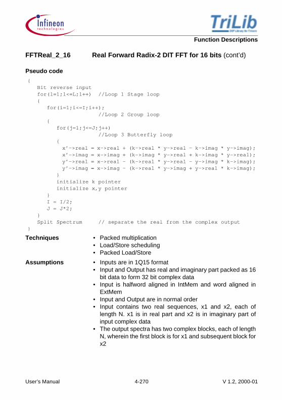
Function Descriptions
Pseudo code
{ Bit reverse input for(l=1;l<=L;l++) //Loop 1 Stage loop { for(i=1;i<=I;i++); //Loop 2 Group loop { for(j=1;j<=J;j++) //Loop 3 Butterfly loop { x’->real = x->real + (k->real * y->real - k->imag * y->imag); x’->imag = x->imag + (k->imag * y->real + k->imag * y->real); y’->real = x->real - (k->real * y->real - y->imag * k->imag); y’->imag = x->imag - (k->real * y->imag + y->real * k->imag); } initialize k pointer initialize x,y pointer } I = I/2; J = J*2; } Split Spectrum // separate the real from the complex output}
Techniques • Packed multiplication• Load/Store scheduling• Packed Load/Store
Assumptions • Inputs are in 1Q15 format• Input and Output has real and imaginary part packed as 16
bit data to form 32 bit complex data• Input is halfword aligned in IntMem and word aligned in
ExtMem• Input and Output are in normal order • Input contains two real sequences, x1 and x2, each of
length N. x1 is in real part and x2 is in imaginary part ofinput complex data
• The output spectra has two complex blocks, each of lengthN, wherein the first block is for x1 and subsequent block forx2
FFTReal_2_16 Real Forward Radix-2 DIT FFT for 16 bits (cont’d)
User’s Manual 4-270 V 1.2, 2000-01

Function Descriptions
Memory Note
Figure 4-71 FFTReal_2_16
FFTReal_2_16 Real Forward Radix-2 DIT FFT for 16 bits (cont’d)
32 bit*
x(1)
x(2)
x(3)
x(4)
.
.
x(0)
x(N-1)
Bitreverseddata fetch
aXInput-Buffer
RFFT
Real andImaginary parts in
1Q15
The data is arranged as inFigure 4-2
HiMemory
Alignment of Input &Output Buffers
IntMem - halfword aligned
ExtMem - word aligned
Buffers will have bothReal and Imaginary parts
Twiddle-Factor
32 bit*
TF(1)
TF(2)
.
.
.
.
TF(0)
TF(N/2-1)
aTF
Output-SpectrumaR
32 bit*
R(1)
R(2)
R(3)
R(4)
.
.
R(0)
R(N-1)Split
Spectrum
Real andImaginary parts in
1Q15
Complexresults offirst Realsequencestored in
real part ofthe Input-
Buffer
Complexresults of
second Realsequencestored inimaginarypart of the
Input-Buffer
*
*
HiMemory
(16 bit Cplx)
(16 bit Cplx)
(16 bit Cplx)
(16 bit Cplx)
32 bit*
aR
R(1) Real
.
.
.
.
.
R(0) Real
R(N-1) Real
R(N+1) Imag
.
.
.
.
.
R(N) Imag
R(2N-1) Imag
User’s Manual 4-271 V 1.2, 2000-01

Function Descriptions
Implementation Refer Section 4.8.2
Example Trilib\Example\Tasking\Transforms\FFT\expRealFFT_2_16.c, expRealFFT_2_16.cppTrilib\Example\GreenHills\Transforms\FFT\expRealFFT_2_16.cpp, expRealFFT_2_16.cTrilib\Example\GNU\Transforms\FFT\expRealFFT_2_16.c
Cycle Count Initialization : 7
First Pass Loop :
Kernel :
• Stage Loop :
• Group Loop :
• Butterfly :
Post Processing :
Split Spectrum :
Example
N is the number of points of FFT
N Actual Higher limit Lower limit
8 219 224 216
256 9766 9766 8869
Code Size 678 bytes
FFTReal_2_16 Real Forward Radix-2 DIT FFT for 16 bits (cont’d)
7 7 N 2⁄× 2+ +
10 Log2N 1–( )× 2+
+8 N 2⁄ 1–( )× 2+
+ 13or11( ) Log2N 1–( ) N 4⁄× 2+
10 Log2N 1–( )× 2+
8 N 2⁄ 1–( )× 2+
13or11( ) Log2N 1–( ) N 4⁄× 2+
6 4 N 2⁄× 4+ +
14 11 N 2 1–⁄( )× 5+ +
User’s Manual 4-272 V 1.2, 2000-01

Function Descriptions
IFFTReal_2_16 Real Inverse Radix-2 DIT IFFT for 16 bits
Signature short IFFTReal_2_16(CplxS *R,
CplxS *X,
CplxS *TF,
int nX,
int SFlg
);
Inputs X
TF
nXSFlg
:
:
::
Pointer to Input-Buffer of 16 bit complex valuePointer to Twiddle-Factor-Buffer of 16 bit complex value in predefined formatSize of Input-Buffer (power of 2)Indicates scale down the input by 2 if this flag is TRUE
Output R : Pointer to Output-Buffer of 16 bit complex value
Return NF : Scaling factor used for normalization
Description This function computes the Real Inverse Radix-2 decimation-in-time Fast fourier transform on the given input complex array. The detailed implementation is given in the Section 4.8.The Real IFFT is implemented by using the complex IFFT and before processing the input is arranged to form a single valued complex sequence from two complex sequences.
User’s Manual 4-273 V 1.2, 2000-01

Function Descriptions
Pseudo code
{ unify spectrum //Forms a single valued complex sequence from two sequences Bit reverse input for(l=1;l<=L;l++) //Loop 1 Stage loop { for(i=1;i<=I;i++); //Loop 2 Group loop { for(j=1;j<=J;j++) //Loop 3 Butterfly loop { x’->real = x->real + (k->real * y->real - k->imag * y->imag); x’->imag = x->imag + (k->imag * k->real - k->imag * y->real); y’->real = x->real - (k->real * y->real - y->imag * k->imag); y’->imag = x->imag - (k->real * y->imag - y->real * k->imag); } initialize k pointer initialize x,y pointer } I = I/2; J = J*2; } }
Techniques • Packed multiplication• Load/Store scheduling• Packed Load/Store
Assumptions • Inputs are in 1Q15 format• Input and Output has real and imaginary part packed as 16
bit data to form 32 bit complex data• Input is halfword aligned in IntMem and word aligned in
ExtMem• Input and Output are in normal order • Input contains two complex blocks each of length N,
wherein the first block is for x1 and subsequent block is forx2
• The output spectra contains two real sequences x1 and x2,each of length N. x1 is in real part and x2 is in imaginarypart of output complex data
Caution • The input array gets modified after processing
IFFTReal_2_16 Real Inverse Radix-2 DIT IFFT for 16 bits (cont’d)
User’s Manual 4-274 V 1.2, 2000-01

Function Descriptions
Memory Note
Figure 4-72 IFFTReal_2_16
IFFTReal_2_16 Real Inverse Radix-2 DIT IFFT for 16 bits (cont’d)
Bitreverseddata fetch
RIFFT
Real andImaginary parts
in 1Q15
The data is arrangedas in Figure 4-2
Alignment of Input &Output Buffers
IntMem - halfword aligned
ExtMem - word aligned
Buffers will have bothReal and Imaginary
parts
Output-Spectrum
aR
32 bit*
R(1)
R(2)
R(3)
R(4)
.
.
R(0)
R(N-1)
Complexinput
sequenceto
generateX1, the
first Realoutput
sequence
Complexinput
sequenceto generate
X2, thesecond
Real outputsequence
32 bit*
X(1)
X(2)
X(3)
X(4)
.
.
X(0)
X(N-1)
aXInput-Buffer
*
UnifySpectrum
Real andImaginary parts in
1Q15
*
aX
32 bit*
X(1) Real
.
.
.
.
.
X(0) Real
X(N-1) Real
X(N+1) Imag
.
.
.
.
.
X(N) Imag
X(2N-1) Imag
Twiddle-Factor
32 bit*
TF(1)
TF(2)
.
.
.
.
TF(0)
TF(N/2-1)
aTF
Contains X1, thefirst real
sequence inReal part and
X2, the secondReal sequence
in imaginary part
*
HiMemoryHi
Memory
(16 bit Cplx)
(16 bit Cplx)(16 bit Cplx)
(16 bit Cplx)
User’s Manual 4-275 V 1.2, 2000-01

Function Descriptions
Implementation Refer Section 4.8.2
Example Trilib\Example\Tasking\Transforms\FFT\expRealFFT_2_16.c, expRealFFT_2_16.cppTrilib\Example\GreenHills\Transforms\FFT\expRealFFT_2_16.cpp, expRealFFT_2_16.cTrilib\Example\GNU\Transforms\FFT\expRealFFT_2_16.c
Cycle Count Initialization : 6
Unify :
First Pass Loop :
Kernel :
• Stage Loop :
• Group Loop :
• Butterfly :
Post Processing :
Example
N is the number of points of FFT
N Actual Higher limit Lower limit
8 209 219 211
256 8868 9637 8740
Code Size 680 bytes
IFFTReal_2_16 Real Inverse Radix-2 DIT IFFT for 16 bits (cont’d)
5 10 N 2⁄×( ) 2+ +
7 7 N 2⁄×+
10 Log2N 1–( )× 2+
+8 N 2⁄ 1–( )× 2+
+ 13or11( ) Log2N 1–( ) N 4⁄× 2+
10 Log2N 1–( )× 2+
8 N 2⁄ 1–( )× 2+
13or11( ) Log2N 1–( ) N 4⁄× 2+
6 4 N 2⁄× 4+ +
User’s Manual 4-276 V 1.2, 2000-01
Function Descriptions
FFT_2_32 Complex Forward Radix-2 DIT FFT for 32 bits
Signature short FFT_2_32(CplxL *R,
CplxL *X,
CplxL *TF,
int nX
);
Inputs X
TF
nX
:
:
:
Pointer to Input-Buffer of 32 bit complex valuePointer to Twiddle- Factor-Buffer of 32 bit complex value in predefined formatSize of Input-Buffer (power of 2)
Output R : Pointer to Output-Buffer of 32 bit complex value
Return NF : Scaling factor used for normalization
Description This function computes the Complex Forward Radix-2 decimation-in-time Fast fourier transform on the given input complex array. The detailed implementation is given in the Section 4.8.4.
User’s Manual 4-277 V 1.2, 2000-01

Function Descriptions
Pseudo code
{ Bit reverse input for(l=1;l<=L;l++) //Loop 1 Stage loop { for(i=1;i<=I;i++); //Loop 2 Group loop { for(j=1;j<=J;j++) //Loop 3 Butterfly loop { x’->real = x->real + (k->real * y->real - k->imag * y->imag); x’->imag = x->imag + (k->imag * k->real + k->imag * y->real); y’->real = x->real - (k->real * y->real - y->imag * k->imag); y’->imag = x->imag - (k->real * y->imag + y->real * k->imag); } initialize k pointer initialize x,y pointer } I = I/2; J = J*2; }}
Techniques • Packed multiplication• Load/Store scheduling• Packed Load/Store
Assumptions • Inputs are in 1Q31 format• Input and Output has real and imaginary part packed as 32
bit data to form 64 bit complex data• Input is halfword aligned in IntMem and word aligned in
ExtMem• Input and Output are in normal order
FFT_2_32 Complex Forward Radix-2 DIT FFT for 32 bits (cont’d)
User’s Manual 4-278 V 1.2, 2000-01

Function Descriptions
Memory Note
Figure 4-73 FFT_2_32
Implementation Refer Section 4.8.4
FFT_2_32 Complex Forward Radix-2 DIT FFT for 32 bits (cont’d)
64 bit
HiMemory
64 bit
x(1)
x(2)
x(3)
x(4)
.
.
x(0)
x(N-1)
Bitreverseddata fetch
aXInput-Buffer
FFT
Alignment of Input &Output Buffers
IntMem - halfword aligned
ExtMem - word aligned
Buffers will have bothReal and Imaginary parts
Real andImaginary parts in
1Q31
The data is arranged as inFigure 4-3
Twiddle-Factor
TF(1)
TF(2)
.
.
.
.
TF(0)
TF(N/2-1)
aTF
Output-Spectrum
aR
64 bit
R(1)
R(2)
R(3)
R(4)
.
.
R(0)
R(N-1) HiMemory
(32 bit Cplx)
(32 bit Cplx)
(32 bit Cplx)
User’s Manual 4-279 V 1.2, 2000-01

Function Descriptions
Example Trilib\Example\Tasking\Transforms\FFT\expCplxFFT_2_32.c, expCplxFFT_2_32.cppTrilib\Example\GreenHills\Transforms\FFT\expCplxFFT_2_32.cpp, expCplxFFT_2_32.cTrilib\Example\GNU\Transforms\FFT\expCplxFFT_2_32.c
Cycle Count Initialization : 8
First Pass Loop :
Kernel :
• Stage Loop :
• Group Loop :
• Butterfly :
Post Processing : 4
Example
N is the number of points of FFT
N Actual Higher limit Lower limit
8 260 264 244
256 19803 20058 18267
Code Size 350 bytes
FFT_2_32 Complex Forward Radix-2 DIT FFT for 32 bits (cont’d)
7 9 N 2 2+⁄×+
10 Log2N 1–( )× 2+
+7 N 2⁄ 1–( )× 2+
+ 20or18( ) Log2N 1–( ) N 2⁄× 2+
10 Log2N 1–( ) 2+×7 N 2⁄ 1–( )× 2+
20or18( ) Log2N 1–( ) N 2⁄× 2+
User’s Manual 4-280 V 1.2, 2000-01
Function Descriptions
IFFT_2_32 Complex Inverse Radix-2 DIT IFFT for 32 bits
Signature short IFFT_2_32(CplxL *R,
CplxL *X,
CplxL *TF,
int nX
);
Inputs X
TF
nX
:
:
:
Pointer to Input-Buffer of 32 bit complex valuePointer to Twiddle- Factor-Buffer of 32 bit complex value in predefined formatSize of Input-Buffer (power of 2)
Output R : Pointer to Output-Buffer of 32 bit complex value
Return NF : Scaling factor used for normalization
Description This function computes the Complex Inverse Radix-2 decimation-in-time Fast fourier transform on the given input complex array. The detailed implementation is given in the Section 4.8.4.
User’s Manual 4-281 V 1.2, 2000-01

Function Descriptions
Pseudo code
{ Bit reverse input for(l=1;l<=L;l++) //Loop 1 Stage loop { for(i=1;i<=I;i++); //Loop 2 Group loop { for(j=1;j<=J;j++) //Loop 3 Butterfly loop { x’->real = x->real + (k->real * y->real - k->imag * y->imag); x’->imag = x->imag + (k->imag * y->real - k->imag * y->real); y’->real = x->real - (k->real * y->real - y->imag * k->imag); y’->imag = x->imag - (k->real * y->imag - y->real * k->imag); } initialize k pointer initialize x,y pointer } I = I/2; J = J*2; }}
Techniques • Packed multiplication• Load/Store scheduling• Packed Load/Store
Assumptions • Inputs are in 1Q31 format• Input and Output has real and imaginary part packed as 32
bit data to form 64 bit complex data• Input is halfword aligned in IntMem and word aligned in
ExtMem• Input and Output are in normal order
IFFT_2_32 Complex Inverse Radix-2 DIT IFFT for 32 bits (cont’d)
User’s Manual 4-282 V 1.2, 2000-01

Function Descriptions
Memory Note
Figure 4-74 IFFT_2_32
Implementation Refer Section 4.8.4
IFFT_2_32 Complex Inverse Radix-2 DIT IFFT for 32 bits (cont’d)
64 bit
HiMemory
64 bit
X(1)
X(2)
X(3)
X(4)
.
.
X(0)
X(N-1)
Bitreverseddata fetch
aXInput-Buffer
IFFT
Real andImaginary parts in
1Q31
The data is arranged as inFigure 4-3
Twiddle-Factor
TF(1)
TF(2)
.
.
.
.
TF(0)
TF(N/2-1)
aTF
Output-Spectrum
aR
64 bit
R(1)
R(2)
R(3)
R(4)
.
.
R(0)
R(N-1) HiMemory
(32 bit Cplx)
(32 bit Cplx) (32 bit Cplx)
Alignment of Input &Output Buffers
IntMem - halfword aligned
ExtMem - word aligned
Buffers will have bothReal and Imaginary parts
User’s Manual 4-283 V 1.2, 2000-01

Function Descriptions
Example Trilib\Example\Tasking\Transforms\FFT\expCplxFFT_2_32.c, expCplxFFT_2_32.cppTrilib\Example\GreenHills\Transforms\FFT\expCplxFFT_2_32.cpp, expCplxFFT_2_32.cTrilib\Example\GNU\Transforms\FFT\expCplxFFT_2_32.c
Cycle Count Initialization : 8
First Pass Loop :
Kernel :
• Stage Loop :
• Group Loop :
• Butterfly :
Post Processing : 4
Example
N is the number of points of FFT
N Actual Higher limit Lower limit
8 244 264 244
256 18523 20058 18267
Code Size 352 bytes
IFFT_2_32 Complex Inverse Radix-2 DIT IFFT for 32 bits (cont’d)
7 9 N 2 2+⁄×+
10 Log2N 1–( )× 2+
+7 N 2⁄ 1–( )× 2+
+ 20or18( ) Log2N 1–( ) N 2⁄× 2+
10 Log2N 1–( ) 2+×7 N 2⁄ 1–( )× 2+
20or18( ) Log2N 1–( ) N 2⁄× 2+
User’s Manual 4-284 V 1.2, 2000-01

Function Descriptions
FFTReal_2_32 Real Forward Radix-2 DIT FFT for 32 bits
Signature short FFTReal_2_32(CplxL *R,
CplxL *X,
CplxL *TF,
int nX
);
Inputs X
TF
nX
:
:
:
Pointer to Input-Buffer of 32 bit complex valuePointer to Twiddle- Factor-Buffer of 32 bit complex value in predefined formatSize of Input-Buffer (power of 2)
Output R : Pointer to Output-Buffer of 32 bit complex value
Return NF : Scaling factor used for normalization
Description This function computes the Real Forward Radix-2 decimation-in-time Fast fourier transform on the given input complex array. The detailed implementation is given in the Section 4.8.4.
User’s Manual 4-285 V 1.2, 2000-01

Function Descriptions
Pseudo code
{ Bit reverse input for(l=1;l<=L;l++) //Loop 1 Stage loop { for(i=1;i<=I;i++); //Loop 2 Group loop { for(j=1;j<=J;j++) //Loop 3 Butterfly loop { x’->real = x->real + (k->real * y->real - k->imag * y->imag); x’->imag = x->imag + (k->imag * y->real + k->imag * y->real); y’->real = x->real - (k->real * y->real - y->imag * k->imag); y’->imag = x->imag - (k->real * y->imag + y->real * k->imag); } initialize k pointer initialize x,y pointer } I = I/2; J = J*2; } Split Spectrum // separate the real from the complex output
}
Techniques • Packed multiplication• Load/Store scheduling• Packed Load/Store
Assumptions • Inputs are in 1Q31 format• Input and Output has real and imaginary part packed as 32
bit data to form 64 bit complex data• Input is halfword aligned in IntMem and word aligned in
ExtMem• Input and Output are in normal order • Input contains two real sequences, x1 and x2, each of
length N. x1 is in real part and x2 is in imaginary part ofinput complex data
• The output spectra has two complex blocks, each of lengthN, wherein the first block is for x1 and subsequent block forx2
FFTReal_2_32 Real Forward Radix-2 DIT FFT for 32 bits (cont’d)
User’s Manual 4-286 V 1.2, 2000-01

Function Descriptions
Memory Note
Figure 4-75 FFTReal_2_32
FFTReal_2_32 Real Forward Radix-2 DIT FFT for 32 bits (cont’d)
64 bit*
x(1)
x(2)
x(3)
x(4)
.
.
x(0)
x(N-1)
Bitreverseddata fetch
aXInput-Buffer
RFFT
Real andImaginary parts in
1Q31
The data is arranged as inFigure 4-3
HiMemory
Alignment of Input &Output Buffers
IntMem - halfword aligned
ExtMem - word aligned
Buffers will have bothReal and Imaginary parts
Twiddle-Factor
64 bit*
TF(1)
TF(2)
.
.
.
.
TF(0)
TF(N/2-1)
aTF
Output-SpectrumaR
64 bit*
R(1)
R(2)
R(3)
R(4)
.
.
R(0)
R(N-1)Split
Spectrum
Real andImaginary parts in
1Q31
Complexresults offirst Realsequencestored in
real part ofthe Input-
Buffer
Complexresults of
second Realsequencestored inimaginarypart of the
Input-Buffer
*
*
HiMemory
(32 bit Cplx)
(32 bit Cplx)
(32 bit Cplx)
(32 bit Cplx)
64 bit*
aR
R(1) Real
.
.
.
.
.
R(0) Real
R(N-1) Real
R(N+1) Imag
.
.
.
.
.
R(N) Imag
R(2N-1) Imag
User’s Manual 4-287 V 1.2, 2000-01

Function Descriptions
Implementation Refer Section 4.8.4
Example Trilib\Example\Tasking\Transforms\FFT\expRealFFT_2_32.c, expRealFFT_2_32.cppTrilib\Example\GreenHills\Transforms\FFT\expRealFFT_2_32.cpp, expRealFFT_2_32.cTrilib\Example\GNU\Transforms\FFT\expRealFFT_2_32.c
Cycle Count Initialization : 8
First Pass Loop :
Kernel :
• Stage Loop :
• Group Loop :
• Butterfly :
Post Processing : 4
Split Spectrum :
Example
N is the number of points of FFT
N Actual Higher limit Lower limit
8 302 306 286
256 20837 21092 19301
Code Size 784 bytes
FFTReal_2_32 Real Forward Radix-2 DIT FFT for 32 bits (cont’d)
7 9 N 2 2+⁄×+
10 Log2N 1–( )× 2+
+7 N 2⁄ 1–( )× 2+
+ 20or18( ) Log2N 1–( ) N 2⁄× 2+
10 Log2N 1–( ) 2+×7 N 2⁄ 1–( )× 2+
20or18( ) Log2N 1–( ) N 2⁄× 2+
13 8 N 2 1–⁄( ) 5+×+
User’s Manual 4-288 V 1.2, 2000-01

Function Descriptions
IFFTReal_2_32 Real Inverse Radix-2 DIT IFFT for 32 bits
Signature short IFFTReal_2_32(CplxL *R,
CplxL *X,
CplxL *TF,
int nX,
int SFlg
);
Inputs X
TF
nXSFlg
:
:
::
Pointer to Input-Buffer of 32 bit complex valuePointer to Twiddle- Factor-Buffer of 32 bit complex value in predefined formatSize of Input-Buffer (power of 2)Indicates scale down the input by 2 if this flag is TRUE
Output R : Pointer to Output-Buffer of 32 bit complex value
Return NF : Scaling factor used for normalization
Description This function computes the Real Inverse Radix-2 decimation-in-time Fast fourier transform on the given input complex array. The detailed implementation is given in the Section 4.8.4. The Real IFFT is implemented by using the complex IFFT and before processing the input is arranged to form a single valued complex sequence from two complex sequences.
User’s Manual 4-289 V 1.2, 2000-01

Function Descriptions
Pseudo code
{ unify spectrum //Forms a single valued complex sequence from two sequences Bit reverse input for(l=1;l<=L;l++) //Loop 1 Stage loop { for(i=1;i<=I;i++); //Loop 2 Group loop { for(j=1;j<=J;j++) //Loop 3 Butterfly loop { x’->real = x->real + (k->real * y->real - k->imag * y->imag); x’->imag = x->imag + (k->imag * k->real - k->imag * y->real); y’->real = x->real - (k->real * y->real - y->imag * k->imag); y’->imag = x->imag - (k->real * y->imag - y->real * k->imag); } initialize k pointer initialize x,y pointer } I = I/2; J = J*2; } }
Techniques • Packed multiplication• Load/Store scheduling• Packed Load/Store
Assumptions • Inputs are in 1Q31 format• Input and Output has real and imaginary part packed as 32
bit data to form 64 bit complex data• Input is halfword aligned in IntMem and word aligned in
ExtMem• Input and Output are in normal order • Input contains two complex blocks each of length N,
wherein the first block is for x1 and subsequent block is forx2
• The output spectra contains two real sequences x1 and x2,each of length N. x1 is in real part and x2 is in imaginarypart of output complex data
Caution • The input array gets modified after processing
IFFTReal_2_32 Real Inverse Radix-2 DIT IFFT for 32 bits (cont’d)
User’s Manual 4-290 V 1.2, 2000-01
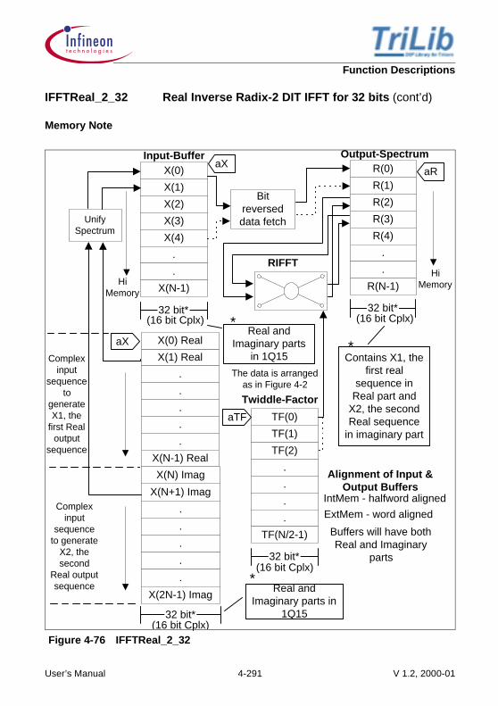
Function Descriptions
Memory Note
Figure 4-76 IFFTReal_2_32
IFFTReal_2_32 Real Inverse Radix-2 DIT IFFT for 32 bits (cont’d)
Bitreverseddata fetch
RIFFT
Real andImaginary parts
in 1Q15
The data is arrangedas in Figure 4-2
Alignment of Input &Output Buffers
IntMem - halfword aligned
ExtMem - word aligned
Buffers will have bothReal and Imaginary
parts
Output-Spectrum
aR
32 bit*
R(1)
R(2)
R(3)
R(4)
.
.
R(0)
R(N-1)
Complexinput
sequenceto
generateX1, the
first Realoutput
sequence
Complexinput
sequenceto generate
X2, thesecond
Real outputsequence
32 bit*
X(1)
X(2)
X(3)
X(4)
.
.
X(0)
X(N-1)
aXInput-Buffer
*
UnifySpectrum
Real andImaginary parts in
1Q15
*
aX
32 bit*
X(1) Real
.
.
.
.
.
X(0) Real
X(N-1) Real
X(N+1) Imag
.
.
.
.
.
X(N) Imag
X(2N-1) Imag
Twiddle-Factor
32 bit*
TF(1)
TF(2)
.
.
.
.
TF(0)
TF(N/2-1)
aTF
Contains X1, thefirst real
sequence inReal part and
X2, the secondReal sequence
in imaginary part
*
HiMemoryHi
Memory
(16 bit Cplx)
(16 bit Cplx)(16 bit Cplx)
(16 bit Cplx)
User’s Manual 4-291 V 1.2, 2000-01

Function Descriptions
Implementation Refer Section 4.8.4
Example Trilib\Example\Tasking\Transforms\FFT\expRealFFT_2_32.c, expRealFFT_2_32.cppTrilib\Example\GreenHills\Transforms\FFT\expRealFFT_2_32.cpp, expRealFFT_2_32.cTrilib\Example\GNU\Transforms\FFT\expRealFFT_2_32.c
Cycle Count Initialization : 8
Unify :
First Pass Loop :
Kernel :
• Stage Loop :
• Group Loop :
• Butterfly :
Post Processing : 4
Example
N is the number of points of FFT
N Actual Higher limit Lower limit
8 298 302 282
256 20833 21088 19297
Code Size 816 bytes
IFFTReal_2_32 Real Inverse Radix-2 DIT IFFT for 32 bits (cont’d)
4 4 N× 2+ +
7 9 N 2 2+⁄×+
10 Log2N 1–( )× 2+
+7 N 2⁄ 1–( )× 2+
+ 20or18( ) Log2N 1–( ) N 2⁄× 2+
10 Log2N 1–( ) 2+×7 N 2⁄ 1–( )× 2+
20or18( ) Log2N 1–( ) N 2⁄× 2+
User’s Manual 4-292 V 1.2, 2000-01
Function Descriptions
FFT_2_16X32 Complex Forward Radix-2 DIT 16 bit mixed FFT
Signature short FFT_2_16X32(CplxS *R,
CplxS *X,
CplxS *TF,
int nX
);
Inputs X
TF
nX
:
:
:
Pointer to Input-Buffer of 16 bit complex valuePointer to Twiddle- Factor-Buffer of 16 bit complex value in predefined formatSize of Input-Buffer (power of 2)
Output R : Pointer to Output-Buffer of 16 bit complex value
Return NF : Scaling factor used for normalization
Description This function computes the Complex Forward Radix-2 decimation-in-time Fast fourier transform on the given input complex array with better precision where it internally uses 32 bit for computation. The detailed implementation is given in the Section 4.8.
User’s Manual 4-293 V 1.2, 2000-01
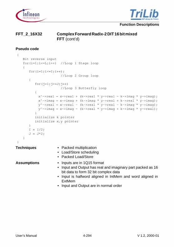
Function Descriptions
Pseudo code
{ Bit reverse input for(l=1;l<=L;l++) //Loop 1 Stage loop { for(i=1;i<=I;i++); //Loop 2 Group loop { for(j=1;j<=J;j++) //Loop 3 Butterfly loop { x’->real = x->real + (k->real * y->real - k->imag * y->imag); x’->imag = x->imag + (k->imag * y->real + k->real * y->imag); y’->real = x->real - (k->real * y->real - k->imag * y->imag); y’->imag = x->imag - (k->real * y->imag + k->imag * y->real); } initialize k pointer initialize x,y pointer } I = I/2; J = J*2; }}
Techniques • Packed multiplication• Load/Store scheduling• Packed Load/Store
Assumptions • Inputs are in 1Q15 format• Input and Output has real and imaginary part packed as 16
bit data to form 32 bit complex data• Input is halfword aligned in IntMem and word aligned in
ExtMem• Input and Output are in normal order
FFT_2_16X32 Complex Forward Radix-2 DIT 16 bit mixed FFT (cont’d)
User’s Manual 4-294 V 1.2, 2000-01

Function Descriptions
Memory Note
Figure 4-77 FFT_2_16X32
Implementation Refer Section 4.8.3
FFT_2_16X32 Complex Forward Radix-2 DIT 16 bit mixed FFT (cont’d)
32 bit
32 bit
x(1)
x(2)
x(3)
x(4)
.
.
x(0)
x(N-1)
Bitreverseddata fetch
aXInput-Buffer
FFT
Real andImaginary parts in
1Q15
The data is arranged as inFigure 4-2
Twiddle-Factor
TF(1)
TF(2)
.
.
.
.
TF(0)
TF(N/2-1)
aTF
Output-Spectrum
aRR(1)
R(2)
R(3)
R(4)
.
.
R(0)
R(N-1)
HiMemory
(16 bit Cplx)
(16 bit Cplx)
Extra spacefor
intermediatecomputation
Alignment of Input &Output Buffers
IntMem - halfword aligned
ExtMem - word aligned
Buffers will have bothReal and Imaginary parts
32 bit(16 bit Cplx)
HiMemory
(2N-1)
(2N-1)
User’s Manual 4-295 V 1.2, 2000-01

Function Descriptions
Example Trilib\Example\Tasking\Transforms\FFT\expCplxFFT_2_16X32.c, expCplxFFT_2_16X32.cppTrilib\Example\GreenHills\Transforms\FFT\expCplxFFT_2_16X32.cpp, expCplxFFT_2_16X32.cTrilib\Example\GNU\Transforms\FFT\expCplxFFT_2_16X32.c
Cycle Count Initialization : 8
First Pass Loop :
Kernel :
• Stage Loop :
• Group Loop :
• Butterfly :
Post Processing :
Example
N is the number of points of FFT
N Actual Higher limit Lower limit
8 269 272 256
256 17508 17508 15712
Code Size 374 bytes
FFT_2_16X32 Complex Forward Radix-2 DIT 16 bit mixed FFT (cont’d)
10 9 nX 2⁄×+
10 Log2N 1–( )× 2+
+7 N 2⁄ 1–( )× 2+
+ 16or14( ) Log2N 1–( ) N 2⁄× 2+
10 Log2N 1–( )× 2+
7 N 2⁄ 1–( ) 2+×16or14( ) Log2N 1–( ) N 2⁄× 2+
11 4 nX×+
User’s Manual 4-296 V 1.2, 2000-01
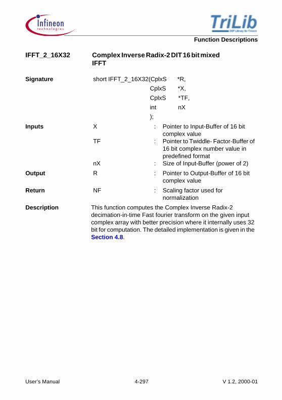
Function Descriptions
IFFT_2_16X32 Complex Inverse Radix-2 DIT 16 bit mixed IFFT
Signature short IFFT_2_16X32(CplxS *R,
CplxS *X,
CplxS *TF,
int nX
);
Inputs X
TF
nX
:
:
:
Pointer to Input-Buffer of 16 bit complex value Pointer to Twiddle- Factor-Buffer of 16 bit complex number value in predefined formatSize of Input-Buffer (power of 2)
Output R : Pointer to Output-Buffer of 16 bit complex value
Return NF : Scaling factor used for normalization
Description This function computes the Complex Inverse Radix-2 decimation-in-time Fast fourier transform on the given input complex array with better precision where it internally uses 32 bit for computation. The detailed implementation is given in the Section 4.8.
User’s Manual 4-297 V 1.2, 2000-01
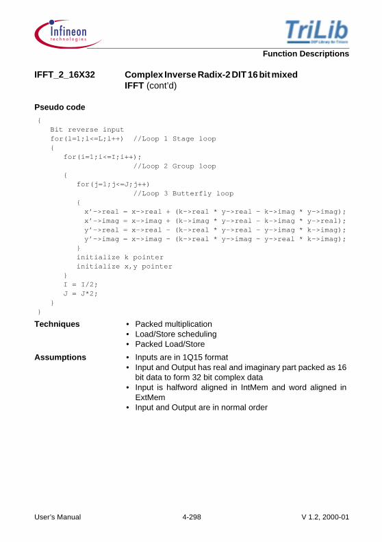
Function Descriptions
Pseudo code
{ Bit reverse input for(l=1;l<=L;l++) //Loop 1 Stage loop { for(i=1;i<=I;i++); //Loop 2 Group loop { for(j=1;j<=J;j++) //Loop 3 Butterfly loop { x’->real = x->real + (k->real * y->real - k->imag * y->imag); x’->imag = x->imag + (k->imag * y->real - k->imag * y->real); y’->real = x->real - (k->real * y->real - y->imag * k->imag); y’->imag = x->imag - (k->real * y->imag - y->real * k->imag); } initialize k pointer initialize x,y pointer } I = I/2; J = J*2; }}
Techniques • Packed multiplication• Load/Store scheduling• Packed Load/Store
Assumptions • Inputs are in 1Q15 format• Input and Output has real and imaginary part packed as 16
bit data to form 32 bit complex data• Input is halfword aligned in IntMem and word aligned in
ExtMem• Input and Output are in normal order
IFFT_2_16X32 Complex Inverse Radix-2 DIT 16 bit mixed IFFT (cont’d)
User’s Manual 4-298 V 1.2, 2000-01

Function Descriptions
Memory Note
Figure 4-78 IFFT_2_16X32
Implementation Refer Section 4.8.3
IFFT_2_16X32 Complex Inverse Radix-2 DIT 16 bit mixed IFFT (cont’d)
32 bit
32 bit
X(1)
X(2)
X(3)
X(4)
.
.
X(0)
X(N-1)
Bitreverseddata fetch
aXInput-Buffer
IFFT
Real andImaginary parts in
1Q15
The data is arranged as inFigure 4-2
Twiddle-Factor
TF(1)
TF(2)
.
.
.
.
TF(0)
TF(N/2-1)
aTF
Output-Spectrum
aRR(1)
R(2)
R(3)
R(4)
.
.
R(0)
R(N-1)
HiMemory
(16 bit Cplx)
(16 bit Cplx)
Extra spacefor
intermediatecomputation
Alignment of Input &Output Buffers
IntMem - halfword aligned
ExtMem - word aligned
Buffers will have bothReal and Imaginary parts
32 bit(16 bit Cplx)
HiMemory
(2N-1)
(2N-1)
User’s Manual 4-299 V 1.2, 2000-01

Function Descriptions
Example Trilib\Example\Tasking\Transforms\FFT\expCplxFFT_2_16X32.c, expCplxFFT_2_16X32.cppTrilib\Example\GreenHills\Transforms\FFT\expCplxFFT_2_16X32.cpp, expCplxFFT_2_16X32.cTrilib\Example\GNU\Transforms\FFT\expCplxFFT_2_16X32.c
Cycle Count Initialization : 8
First Pass Loop :
Kernel :
• Stage Loop :
• Group Loop :
• Butterfly :
Post Processing :
Example
N is the number of points of FFT
N Actual Higher limit Lower limit
8 270 272 256
256 17506 17508 15712
Code Size 376 bytes
IFFT_2_16X32 Complex Inverse Radix-2 DIT 16 bit mixed IFFT (cont’d)
10 9 nX 2⁄×+
10 Log2N 1–( )× 2+
+7 N 2⁄ 1–( )× 2+
+ 16or14( ) Log2N 1–( ) N 2⁄× 2+
10 Log2N 1–( )× 2+
7 N 2⁄ 1–( ) 2+×16or14( ) Log2N 1–( ) N 2⁄× 2+
11 4 nX×+
User’s Manual 4-300 V 1.2, 2000-01

Function Descriptions
FFTReal_2_16X32 Real Forward Radix-2 DIT 16 bit mixed FFT
Signature short FFTReal_2_16X32(CplxS *R,
CplxS *X,
CplxS *TF,
int nX
);
Inputs X
TF
nX
:
:
:
Pointer to Input-Buffer of 16 bit complex valuePointer to Twiddle- Factor-Buffer of 16 bit complex value in predefined formatSize of Input-Buffer (power of 2)
Output R : Pointer to Output-Buffer of 16 bit complex value
Return NF : Scaling factor used for normalization
Description This function computes the Real Forward Radix-2 decimation-in-time Fast Fourier Transform on the given input complex array with better precision where it internally uses 32 bit for computation. The detailed implementation is given in the Section 4.8. The Real FFT is implemented by using the complex FFT and the output spectrum is split to separate the Real FFT results.
User’s Manual 4-301 V 1.2, 2000-01

Function Descriptions
Pseudo code
{ Bit reverse input for(l=1;l<=L;l++) //Loop 1 Stage loop { for(i=1;i<=I;i++); //Loop 2 Group loop { for(j=1;j<=J;j++) //Loop 3 Butterfly loop { x’->real = x->real + (k->real * y->real - k->imag * y->imag); x’->imag = x->imag + (k->imag * y->real + k->imag * y->real); y’->real = x->real - (k->real * y->real - y->imag * k->imag); y’->imag = x->imag - (k->real * y->imag + y->real * k->imag); } initialize k pointer initialize x,y pointer } I = I/2; J = J*2; } Split Spectrum // separate the real from the complex output}
Techniques • Packed multiplication• Load/Store scheduling• Packed Load/Store
Assumptions • Inputs are in 1Q15 format• Input and Output has real and imaginary part packed as 16
bit data to form 32 bit complex data• Input is halfword aligned in IntMem and word aligned in
ExtMem• Input and Output are in normal order with the real part
separated from the complex part
FFTReal_2_16X32 Real Forward Radix-2 DIT 16 bit mixed FFT (cont’d)
User’s Manual 4-302 V 1.2, 2000-01
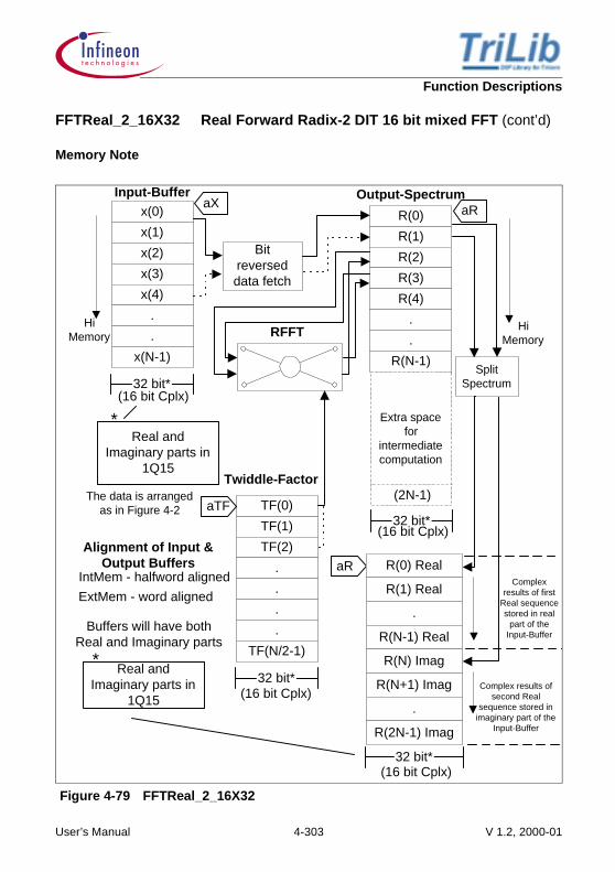
Function Descriptions
Memory Note
Figure 4-79 FFTReal_2_16X32
FFTReal_2_16X32 Real Forward Radix-2 DIT 16 bit mixed FFT (cont’d)
32 bit*
x(1)
x(2)
x(3)
x(4)
.
.
x(0)
x(N-1)
Bitreverseddata fetch
aXInput-Buffer
RFFT
The data is arrangedas in Figure 4-2
HiMemory
Alignment of Input &Output Buffers
IntMem - halfword aligned
ExtMem - word aligned
Buffers will have bothReal and Imaginary parts
Output-SpectrumaR
R(1)
R(2)
R(3)
R(4)
.
.
R(0)
R(N-1)Split
Spectrum
Complexresults of first
Real sequencestored in real
part of theInput-Buffer
Complex results ofsecond Real
sequence stored inimaginary part of the
Input-Buffer
HiMemory
(16 bit Cplx)
(16 bit Cplx)32 bit*
aR R(0) Real
R(1) Real
.
R(N-1) Real
R(N) Imag
R(N+1) Imag
.
R(2N-1) Imag
32 bit*(16 bit Cplx)
Extra spacefor
intermediatecomputation
(2N-1)
Real andImaginary parts in
1Q15
*
Twiddle-Factor
32 bit*
TF(1)
TF(2)
.
.
.
.
TF(0)
TF(N/2-1)
aTF
(16 bit Cplx)
Real andImaginary parts in
1Q15
*
User’s Manual 4-303 V 1.2, 2000-01

Function Descriptions
Implementation Refer Section 4.8.3
Example Trilib\Example\Tasking\Transforms\FFT\expRealFFT_2_16X32.c, expRealFFT_2_16X32.cppTrilib\Example\GreenHills\Transforms\FFT\expRealFFT_2_16X32.cpp, expRealFFT_2_16X32.cTrilib\Example\GNU\Transforms\FFT\expRealFFT_2_16X32.c
Cycle Count Initialization : 8
First Pass Loop :
Kernel :
• Stage Loop :
• Group Loop :
• Butterfly :
Post Processing :
Split Spectrum :
Example
N is the number of points of FFT
N Actual Higher limit Lower limit
8 320 324 308
256 18004 18924 17128
Code Size 662 bytes
FFTReal_2_16X32 Real Forward Radix-2 DIT 16 bit mixed FFT (cont’d)
10 9 nX 2⁄×+
10 Log2N 1–( )× 2+
+7 N 2⁄ 1–( )× 2+
+ 16or14( ) Log2N 1–( ) N 2⁄× 2+
10 Log2N 1–( )× 2+
7 N 2⁄ 1–( ) 2+×16or14( ) Log2N 1–( ) N 2⁄× 2+
11 4 nX×+
14 11 N 2 1–⁄( )× 5+ +
User’s Manual 4-304 V 1.2, 2000-01

Function Descriptions
IFFTReal_2_16X32 Real Inverse Radix-2 DIT 16 bit mixed IFFT
Signature short IFFTReal_2_16X32(CplxS *R,
CplxS *X,
CplxS *TF,
int nX,
int SFlg
);
Inputs X
TF
nXSFlg
:
:
::
Pointer to Input-Buffer of 16 bit complex valuePointer to Twiddle-Factor-Buffer of 16 bit complex value in predefined formatSize of Input-Buffer (power of 2)Indicates scale down the input by 2 if this flag is TRUE
Output R : Pointer to Output-Buffer of 16 bit complex value
Return NF : Scaling factor used for normalization
Description This function computes the Real Inverse Radix-2 decimation-in-time Fast fourier transform on the given input complex array with better precision where it internally uses 32 bit for computation. The detailed implementation is given in the Section 4.8.The Real IFFT is implemented by using the complex IFFT and before processing the input is arranged to form a single valued complex sequence from two complex sequences.
Pseudo code
{ unify spectrum //Forms a single valued complex sequence from two sequences Bit reverse input
User’s Manual 4-305 V 1.2, 2000-01

Function Descriptions
for(l=1;l<=L;l++) //Loop 1 Stage loop { for(i=1;i<=I;i++); //Loop 2 Group loop { for(j=1;j<=J;j++) //Loop 3 Butterfly loop { x’->real = x->real + (k->real * y->real - k->imag * y->imag); x’->imag = x->imag + (k->imag * k->real - k->imag * y->real); y’->real = x->real - (k->real * y->real - y->imag * k->imag); y’->imag = x->imag - (k->real * y->imag - y->real * k->imag); } initialize k pointer initialize x,y pointer } I = I/2; J = J*2; } }
Techniques • Packed multiplication• Load/Store scheduling• Packed Load/Store
Assumptions • Inputs are in 1Q15 format• Input and Output has real and imaginary part packed as 16
bit data to form 32 bit complex data• Input is halfword aligned in IntMem and word aligned in
ExtMem• Input and Output are in normal order with the real part
separated from the complex part• Input contains two complex blocks each of length N,
wherein the first block is for x1 and subsequent block is forx2
• The output spectra contains two real sequences x1 and x2,each of length N. x1 is in real part and x2 is in imaginarypart of output complex data
Caution • The input array gets modified after processing
IFFTReal_2_16X32 Real Inverse Radix-2 DIT 16 bit mixed IFFT (cont’d)
User’s Manual 4-306 V 1.2, 2000-01

Function Descriptions
Memory Note
Figure 4-80 IFFTReal_2_16X32
IFFTReal_2_16X32 Real Inverse Radix-2 DIT 16 bit mixed IFFT (cont’d)
Bitreverseddata fetch
RIFFT
Real andImaginary parts
in 1Q15The data is arranged
as in Figure 4-2
Alignment of Input &Output Buffers
IntMem - halfword aligned
ExtMem - word aligned
Buffers will have bothReal and Imaginary
parts
Output-Spectrum
aRR(1)
R(2)
R(3)
R(4)
.
.
R(0)
R(N-1)
Complexinput
sequenceto
generateX1, the
first Realoutput
sequence
Complexinput
sequenceto generate
X2, thesecond
Real outputsequence
32 bit*
X(1)
X(2)
X(3)
X(4)
.
.
X(0)
X(N-1)
aXInput-Buffer
*
UnifySpectrum
aX
32 bit*
X(1) Real
.
.
.
.
.
X(0) Real
X(N-1) Real
X(N+1) Imag
.
.
.
.
.
X(N) Imag
X(2N-1) Imag
Twiddle-Factor
32 bit*
TF(1)
TF(2)
.
.
.
.
TF(0)
TF(N/2-1)
aTF
Contains X1, thefirst real sequence
in Real part andX2, the second
Real sequence inimaginary part
*
HiMemoryHi
Memory
(16 bit Cplx)
(16 bit Cplx)
(16 bit Cplx)
Extra spacefor
intermediatecomputation
(2N-1)
32 bit*(16 bit Cplx)
Real andImaginary parts in
1Q15
*
User’s Manual 4-307 V 1.2, 2000-01

Function Descriptions
Implementation Refer Section 4.8.3
Example Trilib\Example\Tasking\Transforms\FFT\expRealFFT_2_16X32.c, expRealFFT_2_16X32.cppTrilib\Example\GreenHills\Transforms\FFT\expRealFFT_2_16X32.cpp, expRealFFT_2_16X32.cTrilib\Example\GNU\Transforms\FFT\expRealFFT_2_16X32.c
Cycle Count Initialization : 8
Unify :
First Pass Loop :
Kernel :
• Stage Loop :
• Group Loop :
• Butterfly :
Post Processing :
Example
N is the number of points of FFT
N Actual Higher limit Lower limit
8 314 319 303
256 17004 18795 16999
Code Size 482 bytes
IFFTReal_2_16X32 Real Inverse Radix-2 DIT 16 bit mixed IFFT (cont’d)
5 10 N 2⁄×( ) 2+ +
10 9 nX 2⁄×+
10 Log2N 1–( )× 2+
+7 N 2⁄ 1–( )× 2+
+ 16or14( ) Log2N 1–( ) N 2⁄× 2+
10 Log2N 1–( )× 2+
7 N 2⁄ 1–( ) 2+×16or14( ) Log2N 1–( ) N 2⁄× 2+
11 4 nX×+
User’s Manual 4-308 V 1.2, 2000-01
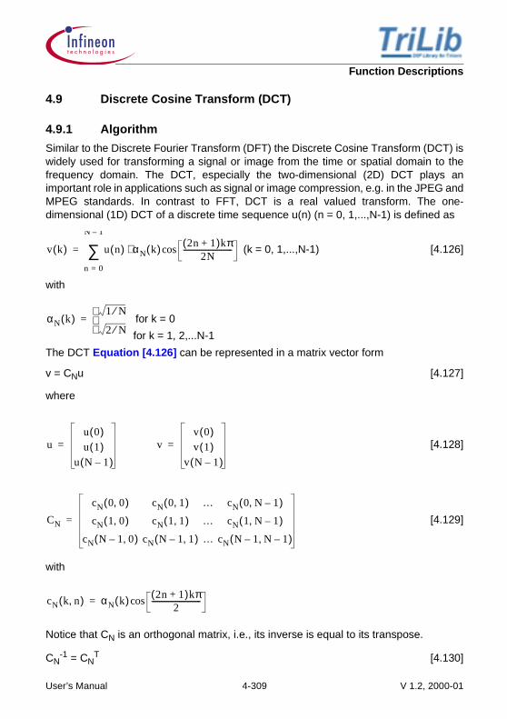
Function Descriptions
4.9 Discrete Cosine Transform (DCT)
4.9.1 Algorithm
Similar to the Discrete Fourier Transform (DFT) the Discrete Cosine Transform (DCT) iswidely used for transforming a signal or image from the time or spatial domain to thefrequency domain. The DCT, especially the two-dimensional (2D) DCT plays animportant role in applications such as signal or image compression, e.g. in the JPEG andMPEG standards. In contrast to FFT, DCT is a real valued transform. The one-dimensional (1D) DCT of a discrete time sequence u(n) (n = 0, 1,...,N-1) is defined as
(k = 0, 1,...,N-1) [4.126]
with
for k = 0
for k = 1, 2,...N-1
The DCT Equation [4.126] can be represented in a matrix vector form
v = CNu [4.127]
where
[4.128]
[4.129]
with
Notice that CN is an orthogonal matrix, i.e., its inverse is equal to its transpose.
CN-1 = CN
T [4.130]
v k( ) u n( ) αN k( ) 2n 1+( )kπ2N
---------------------------cos⋅
n 0=
N 1–
∑=
αN k( )1 N⁄
2 N⁄
=
uu 0( )u 1( )
u N 1–( )= v
v 0( )v 1( )
v N 1–( )=
CN
cN 0 0,( ) cN 0 1,( ) … cN 0 N 1–,( )
cN 1 0,( ) cN 1 1,( ) … cN 1 N 1–,( )
cN N 1– 0,( ) cN N 1– 1,( ) … cN N 1– N 1–,( )
=
cN k n,( ) αN k( ) 2n 1+( )kπ2
---------------------------cos=
User’s Manual 4-309 V 1.2, 2000-01

Function Descriptions
or
CNCNT = CN
TCN = identity matrix
The 2D DCT separates a two dimensional signal (i.e., an image) u(n1, n2), (n1 = 0,1,...,N1-1; n2 = 0, 1,...,N2-1) into parts or spectral subbands of differing importance (withrespect to the visual quality of the image). The transformed image v(n1,n2) has the samesize and is defined as
[4.131]
(k1 = 0, 1,...,N1-1; k2 = 0,1,...,N2-1)
By using the matrix notation
[4.132]
[4.133]
We can write the 2D DCT as a multiplication of three matrices
V = CN1UCN2T
The matrix CN1 and the CN2 are defined as in Equation [4.129].
It is easy to see that the 2D DCT is separable into a sequence of 1D DCTs, N2 times 1DDCTs of the length N1 applied to the columns of U, followed by another N1 times 1DDCTs of the length N2 applied to the rows of CN1U. Hence, we can say that the 1D DCTalgorithm is the Kernel of the 2D one.
A direct implementation of the DCT given in Equation [4.126] requires NxNmultiplications and additions/subtractions of the same order. Like the DFT, the DCT canbe implemented more efficiently by using a fast algorithm. In the literature many fast DCTalgorithms have been developed “References” on Page 423. Among them, the sparse
N1 N2×
v k1 k2,( ) u n1 n2,( ) αN1 k1( )αN2 k2( )⋅
2n1 1+( )k1π2N1
--------------------------------2n2 1+( )k2π
2N2--------------------------------coscos
n2 0=
N2 1–
∑n1 0=
N1 1–
∑=
U
u 0 0,( ) u 0 1,( ) u 0 N2 1–,( )
u 1 0,( ) u 1 1,( ) u 1 N2 1–,( )
u N1 1– 0,( ) u N1 1– 1,( ) u N1 1– N2 1–,( )
=
V
v 0 0,( ) v 0 1,( ) v 0 N2 1–,( )
v 1 0,( ) v 1 1,( ) v 1 N2 1–,( )
v N1 1– 0,( ) v N1 1– 1,( ) v N1 1– N2 1–,( )
=
N1 N2× N2 N2×
User’s Manual 4-310 V 1.2, 2000-01

Function Descriptions
matrix factorization algorithms decompose the coefficient matrix CN into a product ofseveral sparse matrices in order to reduce the number of multiplications and additions.One such algorithm is proposed in “References” on Page 423. It is applicable to anyDCT whose transform length is a power of 2. For a length N 1D DCT, this algorithmrequires (3N/2)(log2N-1)+2 real additions and Nlog2N-(3N/2)+4 real multiplications.
The number of additions and multiplications for this particular case is 26 and 16. Notethat the input samples u(n) are in natural order while the output samples v’(k) are in bitreversed order. The output samples v’(k) are exactly identical to those defined inEquation [4.126] except for scaling
v(k) = v’(k) (k = 0, 1,...,N-1) [4.134]
= v’(k)/2 for N = 8
DCT is an orthogonal transform. If we decompose the scaling factor 1/2 inEquation [4.134] in two 1/ and scale all butterflies in Figure 4-81 whose branchcoefficients are 1 and -1, by 1/ , all butterflies become an orthogonal transform.
In the following, we use this algorithm to compute an DCT. A C code is given below.It computes actually , 8 sample 1D DCTs, based on the signal flow graph inFigure 4-81. The first 8 DCTs (j = 8) are applied to the 8 columns of the original imageand the last 8 DCTs (j = 1) are applied to the 8 rows of the resulting image. The resultswe obtain correspond to the transformed image V in Equation [4.133] except for ascaling ( )2 = 2/N due to Equation [4.134]. The program is for 16 bit fractional dataand works in an in-place manner. The input image U is stored in the raster scan(row-by-row) order in a buffer of the length 64. The same buffer is also used to store theimmediate result C8U during the processing, as well as the final output V in the sameorder.
2N----
22
8 8×2 8×
2 N⁄8 8×
User’s Manual 4-311 V 1.2, 2000-01

Function Descriptions
Figure 4-81 Signal Flow Graph for an 8-sample 1D DCT
-1
x2
x0
x1
x3
x4
x5
x7
x6
-1
-1
-1
-1
-1
-C π/4C π/16
C π/4
-C π/4
C 3π/16C π/4
-S 3π/16
C π/8
S π/8
C π/4
-S 3π/8
S π/16
C 3π/8
-1-1
C π/4
S 5π/16
C 7π/16
C5 π/16
-S 7π/16
C π/4C π/4
X4
X1
X3
X2
X6
X7
X5
X0
User’s Manual 4-312 V 1.2, 2000-01
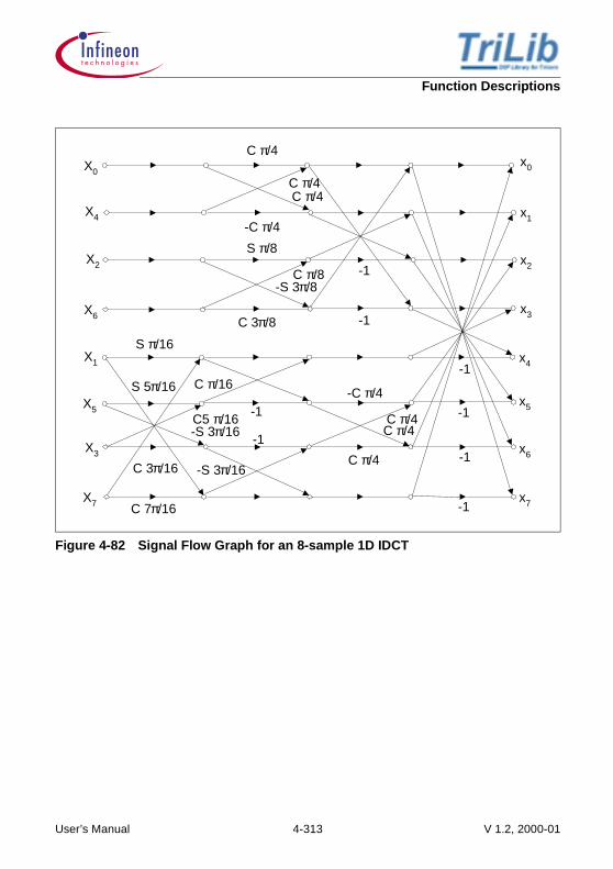
Function Descriptions
Figure 4-82 Signal Flow Graph for an 8-sample 1D IDCT
-1
x2
x0
x1
x3
x4
x5
x7
x6
-1
-1
-1
-1
-1
-C π/4C π/16
C π/4
-C π/4
C 3π/16C π/4
-S 3π/16
C π/8
S π/8
C π/4
-S 3π/8
S π/16
C 3π/8
-1
-1
C π/4
S 5π/16
C 7π/16
C5 π/16 C π/4C π/4
-S 3π/16
X4
X1
X3
X2
X6
X7
X5
X0
User’s Manual 4-313 V 1.2, 2000-01

Function Descriptions
4.10 Inverse Discrete Cosine Transform (IDCT)
4.10.1 Algorithm
The Inverse Discrete Cosine Transform (IDCT) is easily derived from the DCT. Bymultiplying both sides of Equation [4.127] with CN
-1 from left and considering theorthogonality Equation [4.130] we obtain
u = CNTv
or
(n = 0, 1,...,N-1) [4.135]
In other words, to get the IDCT we simply replace the DCT matrix CN by its transposeCN
T. The same is true for the 2D IDCT, i.e.
U = CN1TVCN2
or
[4.136]
(n1 = 0, 1,...,N1-1; n2 = 0,1,...,N2-1)
For the fast computation of IDCT, we use the same idea “References” on Page 423as for DCT. Because each butterfly in Figure 4-81 represents an orthogonal transform(except for a possible scaling), we only need to reserve the signal flow in Figure 4-81in order to get a signal flow graph for IDCT. By introducing the transformed samples v(k)in bit reversed order at the right side, we recover u’(n) in natural order at the left side.The original samples u(n) defined in Equation [4.135] are given by
u(n) = u’(n) (n = 0, 1,...,N) [4.137]
= u’(n)/2 for n = 8
like in Equation [4.134]. The number of additions and multiplications is exactly the sameas for DCT. A C code of 16 bit IDCT is given below. It has the same structure asfor the DCT and differs only in the reversed signal flow.
u n( ) v k( ) αN k( ) 2n 1+( )kπ2N
---------------------------cos⋅
k 0=
N 1–
∑=
u n1 n2,( ) v k1 k2,( ) αN1 k1( )αN2 k2( )⋅
2n1 1+( )k1π2N1
--------------------------------2n2 1+( )k2π
2N2--------------------------------coscos
k2 0=
N2 1–
∑k1 0=
N1 1–
∑=
2N----
8 8×
User’s Manual 4-314 V 1.2, 2000-01

Function Descriptions
4.11 Multidimensional DCT (General Information)
As DCT is a separable transform, 1D DCT, defined in Equation [4.126] can be extendedto 2D DCT as follows.
2D DCT (separable)
[4.138]
u = 0, 1,...,N-1, cl = 1/ l = 0
v = 0, 1,...,M-1, 1,
2D IDCT
[4.139]
n = 0, 1,...,N-1
m = 0, 1,...,M-1,
The normalized version of 2D DCT is
2D DCT (normalized)
[4.140]
u = 0, 1,...,N-1, cl = 1/ l = 0
v = 0, 1,...,M-1, 1,
2D IDCT (normalized)
[4.141]
n = 0, 1,...,N-1
m = 0, 1,...,M-1
Xu v,c2 4
NM----------cucv xn m,
2n 1+( )uπ2N
---------------------------2m 1+( )vπ
2M-----------------------------coscos
m 0=
M 1–
∑n 0=
N 1–
∑=
2
l 0≠
xn m, cucvXu v,c2 2n 1+( )uπ
2N---------------------------
2m 1+( )vπ2M
-----------------------------coscos
v 0=
M 1–
∑u 0=
N 1–
∑=
Xu v,c2
cucv2
NM-------------- xn m,
2n 1+( )uπ2N
---------------------------2m 1+( )vπ
2M-----------------------------coscos
m 0=
∑n 0=
∑=
2N---- cu
n 0=
N 1–
∑ 2
M---------cv xn m,
2m 1+( )vπ2M
-----------------------------cos
m 0=
M 1–
∑ 2n 1+( )uπ2N
---------------------------cos=
2
l 0≠
xn m,2
NM-------------- cucvXu v,
c2 2n 1+( )uπ2N
---------------------------2m 1+( )vπ
2M-----------------------------coscos
v 0=
M 1–
∑u 0=
N 1–
∑=
User’s Manual 4-315 V 1.2, 2000-01
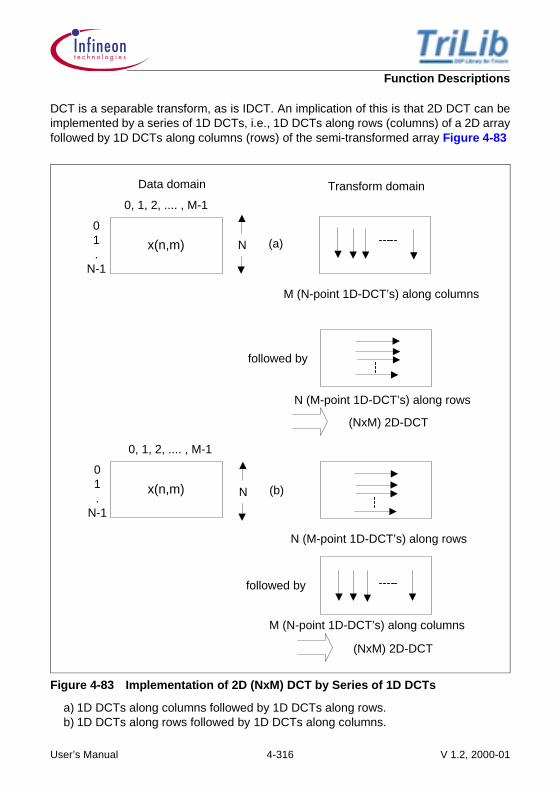
Function Descriptions
DCT is a separable transform, as is IDCT. An implication of this is that 2D DCT can beimplemented by a series of 1D DCTs, i.e., 1D DCTs along rows (columns) of a 2D arrayfollowed by 1D DCTs along columns (rows) of the semi-transformed array Figure 4-83
Figure 4-83 Implementation of 2D (NxM) DCT by Series of 1D DCTs
a) 1D DCTs along columns followed by 1D DCTs along rows.b) 1D DCTs along rows followed by 1D DCTs along columns.
N (M-point 1D-DCT’s) along rows
M (N-point 1D-DCT’s) along columns
01.
N-1
Data domain
0, 1, 2, .... , M-1
x(n,m)
Transform domain
followed by
(NxM) 2D-DCT
followed by
(NxM) 2D-DCT
0, 1, 2, .... , M-1
x(n,m)
N (M-point 1D-DCT’s) along rows
M (N-point 1D-DCT’s) along columns
01.
N-1
N
N
(a)
(b)
User’s Manual 4-316 V 1.2, 2000-01
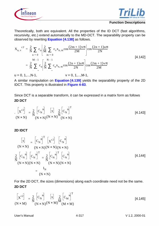
Function Descriptions
Theoretically, both are equivalent. All the properties of the ID DCT (fast algorithms,recursivity, etc.) extend automatically to the MD-DCT. The separability property can beobserved by rewriting Equation [4.138] as follows.
[4.142]
u = 0, 1,...,N-1, v = 0, 1,...,M-1,
A similar manipulation on Equation [4.139] yields the separability property of the 2DIDCT. This property is illustrated in Figure 4-83.
Since DCT is a separable transform, it can be expressed in a matrix form as follows
2D DCT
. [4.143]
2D IDCT
[4.144]
For the 2D DCT, the sizes (dimensions) along each coordinate need not be the same.
2D DCT
[4.145]
Xu v,c2 2
N---- cu
2M----- cvxn m,
2m 1+( )vπ2M
-----------------------------cos
m 0=
∑ 2n 1+( )uπ2N
---------------------------cos
n 0=
∑=
2N---- cu
2N---- cuxn m,
2n 1+( )uπ2N
---------------------------cos
n 0
N 1–
∑ 2m 1+( )vπ2M
-----------------------------cos
m 0
M 1–
∑=
Xc2
N N×( )
2N---- CN
π
N N×( )
x
N N×( )
2N---- CN
πT
N N×( )=
x
N N×( )
CNπ
T
N N×( )
Xc2
N N×( )
CNπ
N N×( )=
2N---- CN
π
N N×( )
CNπ
T
N N×( )
2N---- CN
πT
N N×( )
CNπ
N N×( )=
IN
N N×( )=
Xc2
N M×( )
2N---- CN
π
N N×( )
x
N M×( )
2M----- CM
πT
M M×( )=
User’s Manual 4-317 V 1.2, 2000-01

Function Descriptions
2D IDCT
[4.146]
4.11.1 Descriptions
The following DCT functions are described.
• Discrete Cosine Transform• Inverse Discrete Cosine Transform
4.11.2 2D 8x8 Spatial Block DCT/IDCT Implementation
The DCT, IDCT is implemented using the Chen’s “References” on Page 423 Fast DCT/IDCT one dimensional algorithm which is discussed in the earlier Section 4.10.1. The2D DCT /IDCT exploits the orthogonal property of the algorithm and breaks the 2D 8x8Spatial block into the 8 rows and 8 columns.
Each row is taken as a whole and is processed by the Chen’s ID DCT as inEquation [4.135]and the schematic is shown in the signal flow graph Figure 4-81. Thisis achieved by the RDct1d macro for the DCT and the RIdct1d macro for the IDCT. Thecolumn is then processed by the CDct1d for the DCT and the CIDct1d for the IDCT.
x
N M×( )
CNπ
T
N N×( )
Xc2
N M×( )
CMπ
M M×( )=
2N---- CN
πCN
πT 2
N---- CN
πT
CNπ IN==
2M----- CM
πCM
πT
IM=
User’s Manual 4-318 V 1.2, 2000-01

Function Descriptions
DCT_2_8 Discrete Cosine Transform
Signature DataS* DCT_2_8(DataS *X);
Inputs X : Pointer to Real Data block array Input coefficients
Output None
Return R : Pointer to the Real Data block of DCT coefficient
Description This function implements the 2 dimensional Discrete Cosine Transform. This is implemented using the FDCT algorithm based on the Chen’s, that falls in the class of orthogonal DCTs. The data is organized in the block, the result is returned in the same block.
8 8×
8 8×
8 8×
User’s Manual 4-319 V 1.2, 2000-01

Function Descriptions
Pseudo code
{ int t[12],i,j; for (j=8; j>0; j-=7,d-=8) { t[0] = d[0]; t[1] = d[j]; t[2] = d[2 * j]; t[3] = d[3 * j]; t[4] = d[4 * j]; t[5] = d[5 * j]; t[6] = d[6 * j]; t[7] = d[7 * j];
t[8] = t[0] + t[7]; t[7] = t[0] - t[7]; t[9] = t[1] + t[6]; t[6] = t[1] - t[6]; t[10] = t[2] + t[5]; t[5] = t[2] - t[5]; t[11] = t[3] + t[4]; t[4] = t[3] - t[4];
t[0] = t[8] + t[11]; t[1] = t[8] - t[11]; t[2] = t[9] + t[10]; t[3] = t[9] - t[10];
t[10] = r[0] * (short) (t[6] - t[5]); t[11] = r[0] * (short) (t[6] + t[5]);
t[8] = t[4] + t[10]; t[9] = t[4] - t[10]; t[10] = t[7] + t[11]; t[11] = t[7] - t[11];
d[0] = (r[0] * (short)(t[0] + t[2])) >> 15; d[j] = (r[3] * t[11] + r[4] * t[8]) >> 15; d[2 * j] = (r[1] * t[1] + r[2] * t[3]) >> 15; d[3 * j] = (r[5] * t[10] - r[6] * t[9]) >> 15; d[4 * j] = (r[0] * (short)(t[0] - t[2])) >> 15; d[5 * j] = (r[6] * (t[10] + r[5] * t[9]) >> 15; d[6 * j] = (r[2] * t[1] - r[1] * t[3]) >> 15; d[7 * j] = (r[4] * t[11] - r[3] * t[8]) >> 15;
DCT_2_8 Discrete Cosine Transform (cont’d)
User’s Manual 4-320 V 1.2, 2000-01
Function Descriptions
}}
Techniques • Packed multiplication/addition• Software pipelining• Load/Store scheduling• Packed Load/Store
Assumptions • Input is real sign extended data packed in 16 bit • Output is the sign extended data shifted to left by 3 bit
positions and packed in 16 bits• Input is halfword aligned in IntMem and word aligned in
ExtMem• The processing is done inplace so the input block itself gets
modified by the program• Dynamic Input range is -2048 to 2047 before scaling
DCT_2_8 Discrete Cosine Transform (cont’d)
User’s Manual 4-321 V 1.2, 2000-01

Function Descriptions
Memory Note
Figure 4-84 DCT_2_8
DCT_2_8 Discrete Cosine Transform (cont’d)
8 columns
8rows
16bit
rowi
DCT-Row
DCT-Column
0
1
2
3
4
5
0
7
6
1 2 3 4 5 6 7
1
2
3
4
5
0
7
6
16 bit 8x8 2Dimensional Block
i i+1Note: Input spatial block has to be
scaled up by 8
User’s Manual 4-322 V 1.2, 2000-01

Function Descriptions
Implementation Section 4.11.2
Example Trilib\Example\Tasking\Transforms\DCT\expDCT_2_8.c, expDCT_2_8.cppTrilib\Example\GreenHills\Transforms\DCT\expDCT_2_8.cpp, expDCT_2_8.cTrilib\Example\GNU\Transforms\DCT\expDCT_2_8.c
Cycle Count Initialization : 4
Kernel : 453
Post Processing : 3
Code Size 444 bytes
DCT_2_8 Discrete Cosine Transform (cont’d)
User’s Manual 4-323 V 1.2, 2000-01

Function Descriptions
IDCT_2_8 Inverse Discrete Cosine Transform
Signature DataS* IDCT_2_8(DataS *X);
Inputs X : Pointer to Real Data block array Input coefficients
Output None
Return R : Pointer to the Real Data block of DCT coefficient
Description This function implements the 2D Inverse Discrete Cosine Transform. This is implemented using the FIDCT algorithm based on the Chen’s, that falls in the class of orthogonal DCTs. The data is organized in the block, the result is returned in the same block.
8 8×
8 8×
8 8×
User’s Manual 4-324 V 1.2, 2000-01

Function Descriptions
Pseudo code
{ int t[12],i,j; for (j=8; j>0; j-=7,d-=8) { t[0] = d[0]; t[1] = d[j]; t[2] = d[2 * j]; t[3] = d[3 * j]; t[4] = d[4 * j]; t[5] = d[5 * j]; t[6] = d[6 * j]; t[7] = d[7 * j];
t[8] = (r[4] * t[1] - r[3] * t[7]) >> 15; t[9] = (r[3] * t[1] + r[4] * t[7]) >> 15; t[10] = (r[5] * t[5] - r[6] * t[3]) >> 15; t[11] = (r[6] * t[5] + r[5] * t[3]) >> 15; t[1] = (r[0] * (short) (t[0] + t[4])) >> 15; t[3] = (r[0] * (short) (t[0] - t[4])) >> 15; t[5] = (r[2] * t[2] - r[1] * t[6]) >> 15; t[7] = (r[1] * t[2] + r[2] * t[6]) >> 15;
t[0] = t[1] + t[7]; t[2] = t[1] - t[7]; t[4] = t[3] + t[5]; t[6] = t[3] - t[5];
t[1] = t[8] + t[10]; t[3] = t[8] - t[10]; t[5] = t[9] - t[11]; t[7] = t[9] - t[11];
t[10] = r[0] * (short) (t[5] - t[3]) >> 15; t[11] = r[0] * (short) (t[5] + t[3]) >> 15;
d[0] = t[0] + t[7]; d[j] = t[4] + t[11]; d[2 * j] = t[6] + t[10]; d[3 * j] = t[2] + t[1]; d[4 * j] = t[2] - t[1];
IDCT_2_8 Inverse Discrete Cosine Transform (cont’d)
User’s Manual 4-325 V 1.2, 2000-01

Function Descriptions
d[5 * j] = t[6] - t[10]; d[6 * j] = t[4] - t[11]; d[7 * j] = t[0] - t[7]; }}
Techniques • Packed multiplication/additions• Load/Store scheduling• Packed Load/Store
Assumptions • Input is real sign extended data packed in 16 bit and has tobe scaled up by a factor of 8 (left shifted by 3)
• Output is the sign extended data packed in the 16 bit • Input is halfword aligned in IntMem and word aligned in
ExtMem• The processing is done inplace so the input block itself gets
modified by the program• Dynamic Input range is -2048 to 2047 before scaling
IDCT_2_8 Inverse Discrete Cosine Transform (cont’d)
User’s Manual 4-326 V 1.2, 2000-01

Function Descriptions
Memory Note
Figure 4-85 IDCT_2_8
IDCT_2_8 Inverse Discrete Cosine Transform (cont’d)
8 columns
8rows
16bit
rowi
IDCT-Row
IDCT-Column
0
1
2
3
4
5
0
7
6
1 2 3 4 5 6 7
1
2
3
4
5
0
7
6
16 bit 8x8 2Dimensional Block
i i+1Note: Input spatial block has to be
scaled up by 8
User’s Manual 4-327 V 1.2, 2000-01

Function Descriptions
Implementation Section 4.11.2
Example Trilib\Example\Tasking\Transforms\DCT\expDCT_2_8.c, expDCT_2_8.cppTrilib\Example\GreenHills\Transforms\DCT\expDCT_2_8.cpp, expDCT_2_8.cTrilib\Example\GNU\Transforms\DCT\expDCT_2_8.c
Cycle Count Initialization : 4
Kernel : 439
Post Processing : 3
Code Size 430 bytes
IDCT_2_8 Inverse Discrete Cosine Transform (cont’d)
User’s Manual 4-328 V 1.2, 2000-01

Function Descriptions
4.12 Mathematical Functions
4.12.1 Functions using Polynomial Approximation
The Mathematical and Trignometrical functions can be approximated by polynomialexpansion. Generally, Taylor & McLaren series are used for expansion of thesefunctions. The function uses the coefficients calculated by statistical analysis techniqueof regression. Only limited terms of series are used. To improve the accuracy of theoutput of the function, the optimized coefficients are used.
4.12.1.1 Descriptions
The following series functions are described.
• Sine• Cosine• Arctan• Square Root• Natural log• Natural Antilog• Exponential• X Power Y
User’s Manual 4-329 V 1.2, 2000-01

Function Descriptions
Sine_32 Sine
Signature DataS Sine_32(int X);
Inputs X : The radian input in [-pi,pi] range
Output None
Return R : Output sine value of the function
Description This function calculates the sine of an angle. It takes 32 bit input which represents the angle in radians and returns the 16 bit sine value.
Pseudo code
{ int Xabs; //Stores Absolute value int sign; //sign of the result frac32 XbyPi; //angle scaled down by pi frac32 acc; //Output of polynomial calculation in 4Q28 format frac32 Rf; //32-bit Sine value in 1Q31 frac16 R; //Result in 1Q15 format
Xabs = |X|; if (Xabs != X) sign = 1; //sign = 1 if X is in III or IV quadrant
if (Xabs > Pi/2) Xabs = Pi - Xabs; //if input angle in II or III quadrant subtract //absolute value from pi XbyPi = Xabs (*) one_Pi; //angle is scaled down by pi before being used in the //polynomial calculation acc = ((((H[4] (*) XbyPi + H[3]) (*) XbyPi + H[2]) (*) XbyPi + H[1]) (*) XbyPi + H[0]) (*) XbyPi; //polynomial calculation - acc in 4Q28 format acc = acc << 3; //acc in 1Q31 format if (sign == 1) Rf = 0 - acc; //sine is negative in III and IV quadrant R = (frac16)Rf; //16 bit result in 1Q15 format return R; //Returns the calculated sine value }
Techniques • Use of MAC instructions• Instruction ordering provided for zero overhead Load/Store
Assumptions • Input is the radian value in 3Q29 format, output is the sinevalue in 1Q15 format and coefficients are in 4Q28 format
User’s Manual 4-330 V 1.2, 2000-01

Function Descriptions
Memory Note None
Implementation Sin(x), where x is in radians is approximated using the polynomial expansion.
[4.147]
radians.
Sine value in other quadrants is computed by using the relations,
and
The function takes 32 bit radian input in 3Q29 format to accommodate the range . The output is 16 bits in 1Q15 format. Coefficients are stored in 4Q28 format. Constants pi, pi/2 and 1/pi are also stored in the data segment in 3Q29, 3Q29 and 1Q31 formats respectively.
The absolute value of the radian input is calculated. If the input angle is negative (III/IV Quadrant), then sign=1. If absolute value of the angle is greater than pi/2 (II/III Quadrant), it is subtracted from pi. The angle is then scaled down by pi, converted to 1Q31 and used in polynomial calculation. The result is negated, if sign=1 to give the final sine result.
To have an optimal implementation with zero overhead load store, the polynomial in Equation [4.147] is rearranged as below.
[4.148]
Hence, 4 multiply-accumulate and 1 multiply instruction will compute the expression Equation [4.148] with a load of coefficient done in parallel with each of them.
Sine_32 Sine (cont’d)
x( )sin 3.140625 x π⁄( ) 0.02026367 x π⁄( )2+=
5.325196 x π⁄( )3– 0.5446778 x π⁄( )4+
+ 1.800293 x π⁄( )5
0 x π 2⁄≤ ≤
x–( )sin x( )sin–= 180 x–( )sin xsin=
π– π,( )
x( )sin 1.800293(((( x π⁄( ) 0.5446778 ) x π⁄( )+=
5.325196 ) x π⁄( )– 0.02026367 ) x π⁄( )+
+ 3.140625 ) x π⁄( )
User’s Manual 4-331 V 1.2, 2000-01

Function Descriptions
Example Trilib\Example\Tasking\Mathematical\expSine_32.c, expSine_32.cppTrilib\Example\GreenHills\Mathematical\expSine_32.cpp, expSine_32.cTrilib\Example\GNU\Mathematical\expSine_32.c
Cycle Count With DSP Extensions
If input angle is in (I/II Quadrant)
: 15+2
If input angle is in (III/IV Quadrant)
: 18+2
Without DSP EXtensions
If input angle is in (I/II Quadrant)
: 16+2
If input angle is in (III/IV Quadrant)
: 19+2
Code Size 76 bytes
32 bytes (Data)
Sine_32 Sine (cont’d)
User’s Manual 4-332 V 1.2, 2000-01

Function Descriptions
Cos_32 Cosine
Signature DataS Cos_32(int X);
Inputs X : The radian input in [-pi,pi] range
Output None
Return R : Output cosine value of the function
Description This function calculates the cosine of an angle. It takes 32 bit input which represents the angle in radians and returns the 16 bit cosine value.
Pseudo code
{ int Xabs; //absolute value of angle frac32 XbyPi; //angle scaled down by pi frac32 Pi = pi; frac32 one_Pi = 1/pi; //Constant 1/pi in 1Q31 format int sign; //sign of the result frac32 acc; //Output of polynomial calculation in 4Q28 format frac32 Rf; //32-bit Cosine value in 1Q31 frac16 R; //Result in 1Q15 format Xabs = |X|; X = Pi/2 - Xabs; //Complementary angle is calculated Xabs = |X|; if (X != Xabs) sign = 1; //sign = 1 if input angle is in the II or III //quadrant XbyPi = Xabs (*) one_Pi; //angle is scaled down by pi before being used in the //polynomial calculation acc = ((((H[4] (*) XbyPi + H[3]) (*) XbyPi + H[2]) (*) XbyPi + H[1]) (*) XbyPi + H[0]) (*) XbyPi; //polynomial calculation - acc in 4Q28 format Rf = acc << 3; //acc in 1Q31 format if (sign == 1) //cosine value is negative in the II or III quadrant Rf = 0 - acc;
R = (frac16)Rf; //cosine result in 1Q15 format return R; //Returns the calculated cosine value}
Techniques • Use of MAC instructions • Instruction ordering provided for zero overhead Load/Store
User’s Manual 4-333 V 1.2, 2000-01

Function Descriptions
Assumptions • Input is the radian value in 3Q29 format, output is thecosine value in 1Q15 format and coefficients are in 4Q28format
Memory Note None
Implementation Cos(x) is approximated by the same polynomial expression used for sine as .
The function takes 32 bit radian input in 3Q29 format to accommodate the range . The output is 16 bits in 1Q15 format. Coefficients are stored in 4Q28 format. Constants pi, pi/2 and 1/pi are also stored in the data segment in 3Q29, 3Q29 and 1Q31 formats respectively.
Absolute value of the radian input is calculated. Its complementary angle is determined. If the complementary angle is negative, the input angle is in II/III Quadrant where cos is negative. Hence sign=1. The absolute value of complementary angle is scaled down by pi, brought to 1Q31 format and is used in the polynomial calculation. If sign=1, the result of the polynomial calculation is negated, to give the final cosine result.
The implementation of the polynomial is optimal with zero overhead Load/Store.
Example Trilib\Example\Tasking\Mathematical\expCos_32.c, expCos_32.cppTrilib\Example\GreenHills\Mathematical\expCos_32.cpp, expCos_32.cTrilib\Example\GNU\Mathematical\expCos_32.c
Cycle Count With DSP Extensions
If input angle is in(I/IV Quadrant)
: 15+2
If input angle is in(III/II Quadrant)
: 18+2
Cos_32 Cosine (cont’d)
x( )cos 90 x–( )sin=
π– π,( )
User’s Manual 4-334 V 1.2, 2000-01

Function Descriptions
Without DSP Extensions
If input angle is in(I/IV Quadrant)
: 16+2
If input angle is in(III/II Quadrant)
: 19+2
Code Size 68 bytes
28 bytes (Data)
Cos_32 Cosine (cont’d)
User’s Manual 4-335 V 1.2, 2000-01

Function Descriptions
Arctan_32 Arctan
Signature short Arctan_32(int X);
Inputs X : tan value in the range [-215, 215)
Output None
Return R : Output arctan value of the function
Description This function calculates the arc tangent of the input. The input to the function is 32 bits. The input range is [-215, 215). The function returns 16 bit value which represents the angle in radians.
User’s Manual 4-336 V 1.2, 2000-01

Function Descriptions
Pseudo code
{ frac32 Xabs; //absolute value of input frac32 X1Q31; //|X| or 1/|X| in 1Q31 format used in the polynomial //calculation frac32 acc; //Output of the polynomial calculation in 1Q31 format int sign; //sign of the result frac32 Rf; //32 bit arctan value in 2Q30 format frac16 R; //16 bit arctan result in 2Q14 format Xabs = |X|; if (X != Xabs) sign = 1; //if input tan value is negative,sign = 1
if (Xabs > 1) X1Q31 = 1/Xabs; //X1Q31 = 1/|X| in 1Q31 format if |X| > 1 else X1Q31 = Xabs << 15; //X1Q31 = |X| in 1Q31 format
acc = ((((H[4] (*) X1Q31 + H[3]) (*) X1Q31 + H[2]) (*) X1Q31 + H[1]) (*) X1Q31 + H[0]) (*) X1Q31; //polynomial calculation - acc in 1Q31 format
if (Xabs > 1) acc = 0.5 - acc;//polynomial result is subtracted from 0.5 if //1/|X| has been used in the calculation Rf = acc (*) Pi; //32 bit arctan value in radians - Rf in 2Q30 format R = (frac16)Rf; //16 bit arctan value in radians in 2Q14 format return R; //Returns the calculated arctan value}
Techniques • Use of MAC instructions • Instruction ordering provided for zero overhead Load/Store
Assumptions • Input tan value is in 16Q16 format, output is the angle inradians in 2Q14 format and coefficients are in 1Q31 format
Memory Note None
Arctan_32 Arctan (cont’d)
User’s Manual 4-337 V 1.2, 2000-01

Function Descriptions
Implementation Arctan(x) in radians is approximated using the following polynomial expansion.For x<1,
[4.149]
For the formula
[4.150]
can be used.
As 1/x < 1 (for x>1), the polynomial of Equation [4.149] can be used to compute arctan(1/x).Combining Equation [4.149] and Equation [4.150], For ,
The input to the function is 32 bits in 16Q16 format. Hence input is in the range [-215, 215). The function returns 16 bit output which is the arctan value in radians. Since arctan values lie in the range [-pi/2, pi/2] output format is 2Q14. 32 bits are used to store coefficients in 1Q31 format in the data segment. value is also stored in 3Q29 format in data segment. The absolute value of the input is taken in a register and if input is less than 0, sign is set to 1. When input is less than 1, the upper 16 bits of absolute value will be zero and the lower 16 bits represent the tan value in 0Q16. Shifting 15 times to the left will bring the input to 1Q31 format. This value is used in polynomial calculation. The output of the polynomial is multiplied by and if sign=1, the result is negated to give the final arctan result.
If , the reciprocal is calculated by dividing a one in 16Q16 format by the given input. The result gives reciprocal of input in 0Q32, which is converted to 1Q31. This value is now used in the polynomial calculation.
Arctan_32 Arctan (cont’d)
arc x( )tan π 0.318253x 0.003314x2
0.130908x3
–+(=
+ 0.068542x4
0.009159x5 )–
x 1≥
arc x( )tan π 2⁄ arc 1 x⁄( )tan–=
x 1≥arc x( )tan π 0.5 arc 1 x⁄( )tan–( )=
π
π
x 1>
User’s Manual 4-338 V 1.2, 2000-01

Function Descriptions
The result of the polynomial calculation is subtracted from 0.5 and then multiplied by pi. Once again, it is negated if sign =1 to give the final arctan result in radians.
The implementation of the polynomial is optimal with zero overhead Load/Store.
Example Trilib\Example\Tasking\Mathematical\expArctan_32.c, expArctan_32.cppTrilib\Example\GreenHills\Mathematical\expArctan_32.cpp, expArctan_32.cTrilib\Example\GNU\Mathematical\expArctan_32.c
Cycle Count For |X| < 1 and X > 0 : 28+2
For |X| < 1 and X < 0 : 31+2
For |X| > 1 and X > 0 : 50+2
For |X| > 1 and X < 0 : 53+2
Code Size 126 bytes
24 bytes(Data)
Arctan_32 Arctan (cont’d)
User’s Manual 4-339 V 1.2, 2000-01

Function Descriptions
Sqrt_32 Square Root
Signature short Sqrt_32(int X);
Inputs X : Real input value in the range[0, 214)
Output None
Return R : Output value of the function
Description This function calculates the square root of a given number. It takes 32 bit input in the range [0, 214) and returns 16 bit square root value in the range [0, 27).
User’s Manual 4-340 V 1.2, 2000-01

Function Descriptions
Pseudo code
{ int Shcnt; //Shift count int Scale; //Scaling factor frac32 acc; //Result of Polynomial calculation frac32 X1Q31; //Input scaled to 1Q31 format frac16 R; //Result in 8Q8 format Shcnt = count_lead_sign(X); // number of leading sign values Scale = Shcnt - 15;//Get the scale factor X1Q31 = X << Shcnt;// 1Q31 <- 16Q16 acc = ((((H5 (*) X1Q31 + H4) (*) X1Q31 + H3) (*) X1Q31 + H2) (*) X1Q31 + H1) (*) X1Q31 + H0 //polynomial calculation - acc in 1Q31 format //Input less than 1 if (Scale >= 0) { acc = acc (*) SqrtTab[Scale]; //acc = acc * Scale factor R = (frac16) acc >> 22; //8Q8 format <- 2Q30 format } //Input greater than 1 else { acc = acc (*) SqrtTab[ShCnt+1]; //acc = acc * Scale factor R = (frac16) acc >> 14; //8Q8 format <- 10Q22 format } return R; //Returns the calculated square root}
Techniques • Use of MAC instructions• Instruction ordering for zero overhead Load/Store
Assumptions • Inputs are in 16Q16 format and returned output is in 8Q8format
• Input is always positive
Memory Note None
Sqrt_32 Square Root (cont’d)
User’s Manual 4-341 V 1.2, 2000-01

Function Descriptions
Implementation The square root of the input value x can be calculated by using the following approximation series.
[4.151]
where,
The coefficients of polynomial are stored in 2Q30 format. The square root table (table of scale factors) stores in 1Q31 format where n ranges from 0 to 15. This is same as
in 9Q23 format, where n ranges from 16 to 1. The 32 bit input given is in 16Q16 format which can take values in the range [-215, 215). As input should be positive it will be subset of actual input range, i.e., it is in the range [0, 215). The 16 bit output returned is in 8Q8 format. So the output values are in the range of [0, 27). So it can accommodate inputs in the range [0, 214).
As the polynomial expansion needs input only in the range 0.5 to 1, the given input has to be scaled up or scaled down. If the given input number is greater than 1, then it is scaled down by powers of two, so that scaled input value lies in the range 0.5 to 1.This scaled input is used in polynomial calculation. The calculated output is scaled up by power of to get the actual output.
If the input is less than 1, then it is scaled up by power of two, so that scaled value lies in the range 0.5 to 1. This scaled input is used in polynomial calculation. The calculated output is scaled down by power of to get actual output.
The CLS instructions of TriCore gives directly the shiftcount, to scale up or scale down the input. When input is shifted by this count, it is brought into 1Q15 format. If shiftcount is15, input already exists in the range of 0.5 to 1. If shiftcount is less than 15, indicates input is greater than 1 and has to be scaled down.
Sqrt_32 Square Root (cont’d)
sqrt x( ) 1.454895x 1.34491x2
– 1.106812x3
+=
0.536499x4
– 0.1121216x5
0.2075806+ +
0.5 x 1≥ ≥
1 2⁄( )n
2( )n
2
1 2⁄
User’s Manual 4-342 V 1.2, 2000-01
Function Descriptions
If shiftcount is greater than 15, indicates input is less than 1 and has to be scaled up.
Scale factor is obtained as (15-shiftcount). The output of polynomial calculation is scaled by a value from square root table. The appropriate scale factor is obtained and multiplied to get the square root of given input.
The implementation of the polynomial is optimal with zero overhead Load/Store.
Example Trilib\Example\Tasking\Mathematical\expSqrt_32.c, expSqrt_32.cppTrilib\Example\GreenHills\Mathematical\expSqrt_32.cpp, expSqrt_32.cTrilib\Example\GNU\Mathematical\expSqrt_32.c
Cycle Count If X>1 : 14+2
If X<=1 : 16+2
Code Size 88 byes
88 bytes(Data)
Sqrt_32 Square Root (cont’d)
User’s Manual 4-343 V 1.2, 2000-01

Function Descriptions
Ln_32 Natural logarithm
Signature short Ln_32(int X);
Inputs X : Real input value in the range [2-16, 215)
Output None
Return R : Output value of the function
Description This function calculates logarithm of a function to the base e, i.e., natural logarithm. It takes 32 bit input in the range[2-16, 215) and returns the output logarithm in the range [-24, 24).
User’s Manual 4-344 V 1.2, 2000-01

Function Descriptions
Pseudo code
{ int Shcnt //Shift count int Scale; //Scaling factor frac32 acc; //Result of Polynomial calculation frac32 Xu1Q31; //Input scaled to unsigned 1Q31 format frac32 Xsub1; //X-1 frac32 Rf; //Output of polynomial calculation frac16 R; //Result in 5Q11 format Shcnt = count_lead_sign(X); // number of leading sign values Scale = 14 - Shcnt;//Get the scale factor Shcnt = Shcnt + 1; //add 1 to shift count to bring input to //1 to 2(unsigned 1Q15)from 0.5 to 1 Xu1Q31 = X << Shcnt; //unsigned 1Q15 <- 16Q16 Xsub1 = Xu1Q31 - 1;//X = X - 1
acc = ((((H4 * Xsub1 + H3) * Xsub1 + H2) * Xsub1 + H1) * Xsub1 + H0) * Xsub1 //polynomial calculation - acc in 1Q31 format
acc = acc << 4; //5Q27 <- 1Q31 Add = Scale (*) ln2; //Get the adding factor by scaling Ln2 Add = Add << 12; //5Q27 <- 17Q15
Rf = acc + Add; //Add the factor to get the result in 5Q27 //format R = (frac16)Rf; //result in 5Q11 format return R; //Returns the calculated natural logarithm}
Techniques • Use of MAC instructions• Instruction ordering for zero overhead Load/Store
Assumptions • Inputs are in 16Q16 format and returned output is in 5Q11format
• Input is always positive
Memory Note None
Ln_32 Natural logarithm (cont’d)
User’s Manual 4-345 V 1.2, 2000-01

Function Descriptions
Implementation The natural logarithm of the input value x can be calculated using the following approximation series.
[4.152]
where, which means
The coefficients of polynomial are stored in 1Q31 format. The constant ln2 is also stored in 1Q31 format.
The 32 bit input is in 16Q16 format which can take values in the range [-215, 215). As input to logarithm should always be positive it will be subset of actual input range, i.e., it is in the range [2-16, 215). The 16 bit output returned format is in 5Q11 format.
As the polynomial expansion needs x in the range 1 to 2, the input has to be scaled up or scaled down. If the given input number is greater than 1, then it is scaled down. If less than 1, it is scaled up by powers of two, so that scaled input lies in the range 1 to 2. One is subtracted from this scaled input and this is used in polynomial calculation.
The scale factor is positive, if input is greater than 1 and negative, if input is less than 1. The CLS instruction of TriCore gives the shiftcount. When the input is shifted by this shiftcount it will be scaled in the range 0.5 to 1. The polynomial expects input to be in the range 1 to 2 (unsigned). So 1 is added to the shiftcount.
Scale factor is obtained as (14-shiftcount). The output of polynomial is added with scale times ln2 to get the natural logarithm of given input.
The implementation of the polynomial is optimal with zero overhead Load/Store.
Ln_32 Natural logarithm (cont’d)
x( )ln 0.9991150 x 1–( ) 0.4899597 x 1–( )2–=
+ 0.2856751 x 1–( )3 0.1330566 x 1–( )4–
+ 0.03137207 x 1–( )5
1 x 2≥ ≥ 0 x 1–( ) 1≥ ≥
User’s Manual 4-346 V 1.2, 2000-01

Function Descriptions
Example Trilib\Example\Tasking\Mathematical\expLn_32.c, expLn_32.cppTrilib\Example\GreenHills\Mathematical\expLn_32.cpp, expLn_32.cTrilib\Example\GNU\Mathematical\expLn_32.c
Cycle Count For all X : 19+2
Code Size 86 bytes
24 bytes (Data)
Ln_32 Natural logarithm (cont’d)
User’s Manual 4-347 V 1.2, 2000-01

Function Descriptions
AntiLn_16 Natural Antilogarithm
Signature int AntiLn_16(short X);
Inputs X : Real Input value in the range [-8, 8)
Output None
Return R : Output value of the function
Description This function calculates antilog of a function. It takes 16 bit input in the range [-23, 23) and returns 32 bit antilog value in the range [2-16, 216).
Pseudo code
{ int Shcnt //Shift count int Scale; //Scaling factor frac32 acc; //Result of Polynomial calculation frac32 Rf; //Result of antilog in Q format frac32 X1Q31; //Input scaled to 1Q31 format int Expow; //Power of calculated polynomial frac32 R; //Result in 16Q16 format Shcnt = count_lead_sign(X); //number of leading sign values X1Q31 = X << Shcnt;//1Q15 <- 4Q12
Scale = 19 - Shcnt;//Get the scale factor
acc = ((((H5 (*) X1Q31 + H4) (*) X1Q31 + H3) (*) X1Q31 + H2) (*) X1Q31 + H1) (*) X1Q31 + H0 //polynomial calculation - acc in 3Q29 format
if(Scale <= 0) { R = acc >> 13; //Final result in 16Q16 format }
User’s Manual 4-348 V 1.2, 2000-01

Function Descriptions
else{ Rf = acc; //Rf <- acc Expow = 1 << Scale; // Get power of e^x1Q31 tmp = Expow - 1; //x^n needs (n-1) multiplications for (i=0;i<tmp;i++) { Rf = Rf (*) acc; //Multiply calculated e^x1Q31 with itself power times }
//Get the shift count to convert final result in 16Q16 format Expow = Expow << 1; ShCnt = Expow - 15;
R = Rf << ShCnt; //Final result in 16Q16 format }
return R; //Returns the calculated natural antilogarithm}
Techniques • Use of MAC instructions• Instruction ordering for zero overhead Load/Store
Assumptions • Input 4Q12 format, output is the antilog of the input in16Q16 format and coefficients are in 3Q29 format
Memory Note None
AntiLn_16 Natural Antilogarithm (cont’d)
User’s Manual 4-349 V 1.2, 2000-01

Function Descriptions
Implementation The antilog of the input value x can be calculated by using the following approximation series.
[4.153]
The coefficients of polynomial are stored in 3Q29 format. The 16 bit input is in 4Q12 format which can take values in the range [-23, 23). The output returned is in 16Q16 format.The input is scaled in the range -1 to +1. If the given number is greater than 1, it is scaled down and if it is less than -1, it is scaled up by powers of 2. This scaled input is used in polynomial calculation.
The CLS instruction of TriCore gives the shiftcount to scale up or scale down the input. Only when shiftcount is less than 19, input is scaled up or scaled down. Otherwise input is in the range -1 to +1. The scale factor is obtained as (19-shiftcount). This scale factor will always be positive for the inputs greater than 1 and less than -1. The output of polynomial calculation is multiplied with itself scale factor times to get the actual output.
The implementation of the polynomial is optimal with zero overhead Load/Store.
Example Trilib\Example\Tasking\Mathematical\expAntiLn_16.c, expAntiLn_16.cppTrilib\Example\GreenHills\Mathematical\expAntiLn_16.cpp, expAntiLn_16.cTrilib\Example\GNU\Mathematical\expAntiLn_16.c
Cycle Count If X in the range -1 to 1
: 14+2
else :
Code Size 104 bytes
24 bytes (Data)
AntiLn_16 Natural Antilogarithm (cont’d)
AntiLn x( ) 1.0000 1.0001x 0.4990x2
0.1705x3
+ ++=
+ 0.0348x4
0.0139x5
+
16 scale 2×( ) 5 2+ + +
User’s Manual 4-350 V 1.2, 2000-01

Function Descriptions
Expn_16 Exponential
Signature short Expn_16(DataS X);
Inputs X : Real Input value in the range [-1, 1)
Output None
Return R : Output exponent value of the function
Description This function calculates the exponent of the given input. It takes 16 bit input in the range [-1, 1) and returns the exponential value in 16 bits.
Pseudo code
{ frac32 acc; //result of polynomial calculation in 3Q29 format frac16 R; //16 bit exponential result in 3Q13 format acc = ((((H[5] (*) X + H[4]) (*) X + H[3]) (*) X + H[2]) (*) X + H[1]) (*) X + H0; //polynomial calculation - acc is result in 3Q29 format R = (frac16)acc; //16 bit exponential result in 3Q13 format}
Techniques • Use of packed data Load/Store• Use of MAC instructions• Instruction ordering for zero overhead Load/Store
Assumptions • Input 1Q15 format, output is the exponential of the input in3Q13 format and coefficients are in 3Q29 format
Memory Note None
Implementation Exp(x) is approximated using the polynomial expansion given below.
[4.154]
The input to the function is 16 bits in 1Q15 format. Hence input range is [-1, 1). Input outside this range should be scaled to this range before calling the function. Coefficients are stored in 3Q29 format. Output of the function is in 3Q13 format.
The polynomial is implemented in an optimal way so as to have zero overhead Load/Store.
x( )exp 1.0000 1.0001x 0.4990x2
0.1705x3
+ ++=
+ 0.0348x4
0.0139x5
+
User’s Manual 4-351 V 1.2, 2000-01

Function Descriptions
Example Trilib\Example\Tasking\Mathematical\expExpn_16.c, expExpn_16.cppTrilib\Example\GreenHills\Mathematical\expExpn_16.cpp, expExpn_16.cTrilib\Example\GNU\Mathematical\expExpn_16.c
Cycle Count 10+2
Code Size 42 bytes
24 bytes (Data)
Expn_16 Exponential (cont’d)
User’s Manual 4-352 V 1.2, 2000-01

Function Descriptions
XpowY_32 X Power Y
Signature int XpowY_32(int X, DataS Y);
Inputs X
Y
:
:
Real input value in the range [2-11, 211)power in the range [-1,1)
Output None
Return R : Output value of the function in the range [2-11, 211)
Description X power Y is calculated. The input is 32-bit in 12Q20 format but it should lie within the range [2-11, 211). The exponentY is 16-bit in 1Q15 format and is in the range [-1,1). The output is 32-bit in 12Q20 format and lies in the range[2-11, 211)
User’s Manual 4-353 V 1.2, 2000-01

Function Descriptions
Pseudo code
{ int Shcnt //Shift count int Scale; //Scaling factor frac32 acc; //Result of Polynomial calculation frac32 Xu1Q31; //Input scaled to unsigned 1Q31 format frac32 Xsub1; //X-1 frac32 Rf; //Output of polynomial calculation frac32 LnX; //Result of ln in 4Q28 format frac32 LnXPowY; //Y*lnX in 4Q28 format int Expow; //Power of calculated polynomial frac32 R; //Result in 12Q20 format Shcnt = count_lead_sign(X); // number of leading sign values Scale = 10 - Shcnt;//Get the scale factor Shcnt = Shcnt + 1; //add 1 to shift count to bring input to //1 to 2(unsigned 1Q15)from 0.5 to 1 Xu1Q31 = X << Shcnt; //unsigned 1Q15 <- 16Q16 Xsub1 = Xu1Q31 - 1;//X = X - 1 if(Xsub1 == 0) go to XpowY_2
acc = ((((H4 * Xsub1 + H3) * Xsub1 + H2) * Xsub1 + H1) * Xsub1 + H0) * Xsub1 //polynomial calculation - acc in 1Q31 format
acc = acc << 3; //4Q28 <- 1Q31
XpowY_2: Scale = Scale << 26; //6Q26 <- 32Q0 Add = Scale (*) ln2; //Get the adding factor by scaling Ln2 Add = Add << 2; //4Q28 <- 6Q26 LnX = acc + Add; //Add the factor to get the result in 4Q28 //format LnXpowY = LnX (*) Y;
Shcnt = count_lead_sign(LnXpowY); //number of leading sign values X1Q31 = LnXpowY << Shcnt;//1Q31 <- 4Q28
XpowY_32 X Power Y (cont’d)
User’s Manual 4-354 V 1.2, 2000-01

Function Descriptions
Scale = 19 - Shcnt;//Get the scale factor
acc = ((((H5 (*) X1Q31 + H4) (*) X1Q31 + H3) (*) X1Q31 + H2) (*) X1Q31 + H1) (*) X1Q31 + H0 //polynomial calculation - acc in 3Q29 format if(Scale <= 0) { R = acc >> 9; //Final result in 12Q20 format
} else { Rf = acc; //Rf <- acc Expow = 1 << Scale; // Get power of e^x1Q31 tmp = Expow - 1; //x^n needs (n-1) multiplications for (i=0;i<tmp;i++) { Rf = Rf (*) acc; //Multiply calculated e^x1Q31 with itself power times } //Get the shift count to convert final result in 12Q20 format Expow = Expow << 1; ShCnt = Expow - 11;
R = Rf << ShCnt; //Final result in 12Q20 format }
return R; //Returns the calculated X power Y}
Techniques • Use of MAC instructions• Instruction ordering for zero overhead Load/Store
Assumptions • Inputs are in 12Q20 format and should in the range [2-11,211) which is a subset of actual range. Exponent is in 1Q15format and is in the range [-1,1).The returned output is in12Q20 format and lies in the range [2-11, 211)
• Input is always positive
Memory Note None
XpowY_32 X Power Y (cont’d)
User’s Manual 4-355 V 1.2, 2000-01

Function Descriptions
Implementation X power Y can be calculated as e(Y.lnX). The natural logarithm of the input value x can be calculated using the following approximation series.
[4.155]
where, which means
The coefficients of polynomial are stored in 1Q31 format. The constant ln2 is also stored in 1Q31 format.
The 32 bit input is in 12Q20 format which can take values in the range [-211, 211). As input to logarithm should always be positive it will be subset of actual input range, i.e., in the range [2-20, 211). For proper operation of lnX and antiln(Y.lnX) input should lie in the range [2-11, 211). The 32 bit output format is 12Q20 which lies in the range [2-11, 211). Implementation of lnX is same as natural logarithm of X except that scale factor is obtained as (10 - shiftcount) [Refer Natural Logarithm].The output (lnX) is multiplied with the exponent Y. The resulting product is in 4Q28 format. The antilog of this product gives the desired output.The antilog of the input value X can be calculated by using the following approximation series.
[4.156]
The coefficients of polynomial are stored in 3Q29 format. The 32 bit input is in 4Q28 format. The output is in 12Q20 format. Implementation is same as natural antilog of function. [Refer Natural Antilog].
XpowY_32 X Power Y (cont’d)
x( )ln 0.9991150 x 1–( ) 0.4899597 x 1–( )2–=
+ 0.2856751 x 1–( )3 0.1330566 x 1–( )4–
+ 0.03137207 x 1–( )5
1 x 2≥ ≥ 0 x 1–( ) 1≥ ≥
AntiLn x( ) 1.0000 1.0001x 0.4990x2
0.1705x3
+ ++=
+ 0.0348x4
0.0139x5
+
User’s Manual 4-356 V 1.2, 2000-01

Function Descriptions
4.12.2 Random Number Generation
Randomness is typically associated with unpredictability. Mathematics provides aprecise definition of randomness that is then applied here to evaluate random numbervector. Random numbers within the context of the function Rand_16 refers to "asequence of independent numbers with a specified distribution and a specifiedprobability of falling in any given range of values".
Example Trilib\Example\Tasking\Mathematical\expXpowY_32.c, expXpowY_32.cppTrilib\Example\GreenHills\Mathematical\expXpowY_32.cpp, expXpowY_32.cTrilib\Example\GNU\Mathematical\expXpowY_32.c
Cycle Count When X is a power of 2 and XY in the range [e-1, e)
38+2
When X is a power of 2 and XY not in the range [e-1, e)
for scale = 1
scale factor for antiln(YlnX)
otherwise
scale factor for antiln(YlnX)
When X is not a power of 2 and XY in the range [e-1, e)
47+2
When X is not a power of 2 and XY not in the range [e-1, e)
for scale = 1
scale factor for antiln(YlnX)
otherwise
scale factor for antiln(YlnX)
Code Size 190 bytes
48 bytes (Data)
XpowY_32 X Power Y (cont’d)
42 2 scale 1 2+ +×+
42 2 scale 2 2+ +×+
51 2 scale 1 2+ +×+
51 2 scale 2 2+ +×+
User’s Manual 4-357 V 1.2, 2000-01

Function Descriptions
Here Random Number Generator is implemented using Linear Congruential Method(L.C.M). RNG using linear congruential method is also called pseudo RNG becausethey require a seed and produce a deterministic sequence of numbers. Algorithm usedhere is called L.C.M introduced by D. Lehmen in 1951.
Linear Congruential Method
This method produces a sequence of integers X1, X2, X3,... between zero and M-1according to the following recursive relationship
i = 0,1,2,... [4.157]
where,
Apart from LCM many Random Number Generators exist, but this method is arguablythe fastest for a 16-bit value. If a 32-bit value is needed, the code can be modified byperforming a 32-bit multiply and using 32-bit constants (RNDMULT, RNDINC). Thismethod, however, does have one major disadvantage. It is very sensitive to the valuesof RNDMULT and RNDINC.
Much research has been done to identify the optimal choices of these constants to avoiddegeneration. The constants used in the subroutine below were chosen based on thisresearch.
M: The modulus value. This routine returns a random number from 0 to 65536 (64K) andis not internally bounded. If the user needs a min/max limit, this must be coded externallyto this routine.
RNDSEED: An arbitrary constant, can be chosen to be any value representable by the(0-64K) word. If zero is chosen, RNDINC should be some larger value than one.Otherwise, the first two values will be zero and one. This is ok if the generator is giventhree cycles to warm up. To change the set of random numbers generated by thisroutine, change the RNDSEED value. RNDSEED=21845 is used in this routine becauseit is 65536/3.
RNDMULT: Should be chosen such that the last three digits are even-2-1 (such asxx821, x421, etc). RNDMULT=31821 is used in this routine.
Xi : the initial value, called the seed
a : constant multiplier (RNDMULT)
c : increment (RNDINC)
M : modulus
Xi 1+ aXi c+( )modM=
User’s Manual 4-358 V 1.2, 2000-01

Function Descriptions
RNDINC: In general, this constant can be any prime number related to M (or 64K in thiscase).Two values were actually tested, 1 and 13849. Research shows that RNDINC (theincrement value) should be chosen by the following formula
[4.158]
Using M=65536, RNDINC=13849. (as indicated above.)
RNDINC=13849 is used in this routine.
Because PRNG’s employ a mathematical algorithm for number generation, all PRNG’spossess the following properties:
• A seed value is required to initialize the equation• The sequence will cycle after a particular period
4.12.2.1 Description
The following Random Number Generation functions are described.
• Random Number Initialization• Random Number Generator
RNDINC 1 2⁄ 1 6⁄ SQRT 3( )×( )–( ) M×( )=
User’s Manual 4-359 V 1.2, 2000-01

Function Descriptions
RandInit_16 Random Number Initialization
Signature void RandInit_16(void);
Inputs None
Output None
Return None
Description RandInit_16 function initializes the value of seed stored inglobal memory location for 16-bit random number generationroutine.
Pseudo code None
Techniques None
Assumptions None
Memory Note
Figure 4-86 RandInit_16
Implementation RndSeed, the seed for Random Vector Generator is initialized from global memory. Assembler directive .space is used to reserve a block of memory. The seed value is stored in this memory. This memory is declared as global so that seed value can be accessed while generating random vector.
Example Trilib\Example\Tasking\Mathematical\expRandInit_16.c,expRandInit_16.cpp
Trilib\Example\GreenHills\Mathematical\expRandInit_16.cpp, expRandInit_16.cTrilib\Example\GNU\Mathematical\expRandInit_16.c
Cycle Count 2+2
Code Size 14 bytes
RandSeedaRndSeed
Declared as Global
User’s Manual 4-360 V 1.2, 2000-01

Function Descriptions
Rand_16 Random Number Generator
Signature void Rand_16(int nX, int *R );
Inputs nX : Size of output vector
R : Pointer to output vector
Output R[nX] : Output vector
Return None
Description Rand_16 function computes vector of 16 bit random numbers.Seed value is initialized by RandInit_16 function. This functionuses 16 bit predefined RandMul, RandInc values to calculateoutput vector of given size. After calculation of random vectorthe seed in memory is updated. So if this function is calledagain, will use this new seed value and vector generated willbe different from the original one.
Pseudo code
{ int i; for (i=0;i<max;i++) { rndvec[i] = (rndseed*rndmul+rndinc)%modulus; //Rndvec=16-bit random number //RndSeed=Seed value=21845,Userdefined constant //RndMul=Multiplier=31821,Userdefined constant //RndInc=Increment=13849, Userdefined constant //Modulus=65536,Userdefined constant } rndseed = rndvec[i];}
Techniques • Instruction ordering for zero overhead Load/Store
Assumptions • Uses seed value from the memory location which can beinitialized by Rand initialization routine
User’s Manual 4-361 V 1.2, 2000-01

Function Descriptions
Memory Note
Figure 4-87 Rand_16
Implementation Random vector generation uses
[4.159]
RndSeed is initialized by routine RandInit_16, rest other constant values are stored immediate to data registers. viz.,RndMul, RndInc, Modulus.Rndseed stored in global memory is accessed as external variable and Random Vector is calculated as per above equation.
Example Trilib\Example\Tasking\Mathematical\expRand_16.c,expRand_16.cpp
Trilib\Example\GreenHills\Mathematical\expRand_16.cpp, expRand_16.cTrilib\Example\GNU\Mathematical\expRand_16.c
Cycle Count With DSP Extensions
Without DSP Extensions
Code Size 38 bytes
Rand_16 Random Number Generator (cont’d)
RandSeedaRndSeed
Initialized in Rndinit
Randvec RndSeed RndMul× RndInc+( )Modulus=
4 nX 8( )× 1 2+ + +
4 nX 8( )× 1 2+ + +
User’s Manual 4-362 V 1.2, 2000-01

Function Descriptions
4.13 Matrix Operations
A matrix is a rectangular array of numbers (or functions) enclosed in brackets. Thesenumbers (or functions) are called entries or elements of the matrix.The number of entriesin the matrix is product of number of rows and columns. An matrix means matrixwith m rows and n columns. In the double-subscript notation for the entries, the firstsubscript always denotes the row and the second the column.
4.13.1 Descriptions
The following Matrix Operations are described.
• Addition• Subtraction• Multiplication• Transpose
m n×
User’s Manual 4-363 V 1.2, 2000-01

Function Descriptions
MatAdd_16 Addition
Signature void MatAdd_16 (short X[ ] [MAXCOL], short Y[ ] [MAXCOL], short R[ ] [MAXCOL], int nRow, int nCol );
Inputs XYR nRownCol
:::::
Pointer to first matrixPointer to second matrixPointer to output matrixNumber of rowsNumber of columns
Output R : Pointer to output matrix which is the sum of the matrices X and Y
Return None
Description This function performs the addition of two matrices. It takes pointers to the two matrices, pointer to the output matrix, size of row and size of column as input. The entries in the matrices are 16 bit values. The output matrix is stored starting from the address which is sent as input.
Pseudo code
{ short *R; //Ptr to a two dimensional output array of nRow //rows and nCol columns int Tmp;
Tmp = nRow * nCol; //number of elements loopCnt = Tmp/4 //4 additions performed per loop for(i=0;i<loopCnt;i+=4) { *(R+i) = *(X+i) + *(Y+i); *(R+i+1) = *(X+i+1) + *(Y+i+1); *(R+i+2) = *(X+i+2) + *(Y+i+2); *(R+i+3) = *(X+i+3) + *(Y+i+3); }}
Techniques • Loop Unrolling, 4 additions/loop• Use of packed data Load/Store• Use of packed addition with saturation• Instruction ordering provided for zero overhead Load/Store
User’s Manual 4-364 V 1.2, 2000-01

Function Descriptions
Assumptions • nRow = 2*m, m = 1,2,3...• nCol = 2*n, n = 1,2,3...
Memory Note
Figure 4-88 MatAdd_16
MatAdd_16 Addition (cont’d)
aX
X[0][1]
.
X[0][nCol-1]
X[1][0]
X[1][1]
.
X[0][0]
X[nRow-1][nCol-1]
+
Input-Buffer-1
short
Y[0][1]
.
Y[0][nCol-1]
Y[1][0]
Y[1][1]
.
Y[0][0]
Y[nRow-1][nCol-1]
+
aY
Input-Buffer-2
R[0][1]
.
R[0][nCol-1]
R[1][0]
R[1][1]
.
R[0][0]
R[nRow-1][nCol-1]
Output-Buffer
aR
short
shortshort
Packedadd
Alignment of Input &Output Buffers
IntMem - halfword aligned
ExtMem - word aligned
User’s Manual 4-365 V 1.2, 2000-01

Function Descriptions
Implementation The inputs to the function are three pointers (one each to each of the input matrices to be added and one to the output matrix) and the number of rows and number of columns. Both number of rows and number of columns are multiple of two. Hence the number of elements could be 4,8,12,.... This fact is made use of in implementing the matrix addition in an optimal manner. Addition is performed in a loop. Using TriCore’s load doubleword instruction, four elements of each matrix are loaded in two data register pairs. Using packed arithmetic on halfwords, two of the 16 bit entries can be added in one cycle. Hence, by using two packed add instructions per loop, the loop count is brought down by a factor of four. The loop is executed (nRow * nCol)/4 times.
Example Trilib\Example\Tasking\Matrix\expMatAdd_16.c, expMatAdd_16.cppTrilib\Example\GreenHills\Matrix\expMatAdd_16.cpp, expMatAdd_16.cTrilib\Example\GNU\Matrix\expMatAdd_16.c
Cycle Count Pre-loop : 5
Loop :
Post-loop : 0+2
Code Size 52 bytes
MatAdd_16 Addition (cont’d)
3 nRow× nCol×4
------------------------------------------- 2+
User’s Manual 4-366 V 1.2, 2000-01

Function Descriptions
MatSub_16 Subtract
Signature void MatSub_16(short X[ ] [MAXCOL], short Y[ ] [MAXCOL], short R[ ] [MAXCOL], int nRow, int nCol );
Inputs XYRnRownCol
:::::
Pointer to first matrixPointer to second matrixPointer to output matrixNumber of rowsNumber of columns
Output R : Pointer to output matrix which is the subtraction of the matrices X and Y
Return None
Description This function performs the subtraction of two matrices. It takes pointers to the two matrices, pointer to the output matrix, size of row and size of column as input. The entries in the matrices are 16 bit values. The output matrix is stored starting from the address which is sent as input.
Pseudo code
{ short *R; //Ptr to a two dimensional output array of nRow //rows and nCol columns int Tmp;
Tmp = nRow * nCol; //number of elements loopCnt = Tmp/4 //4 subtractions performed per loop
for(i=0;i<loopCnt;i+=4) { *(R+i) = *(X+i) - *(Y+i); *(R+i+1) = *(X+i+1) - *(Y+i+1); *(R+i+2) = *(X+i+2) - *(Y+i+2); *(R+i+3) = *(X+i+3) - *(Y+i+3); }}
User’s Manual 4-367 V 1.2, 2000-01

Function Descriptions
Techniques • Loop Unrolling, 4 subtractions/loop• Use of packed data Load/Store• Use of packed subtraction with saturation• Instruction ordering provided for zero overhead Load/Store
Assumptions • nRow = 2*m, m = 1,2,3...• nCol = 2*n, n = 1,2,3...
MatSub_16 Subtract (cont’d)
User’s Manual 4-368 V 1.2, 2000-01

Function Descriptions
Memory Note
Figure 4-89 MatSub_16
MatSub_16 Subtract (cont’d)
aX
X[0][1]
.
X[0][nCol-1]
X[1][0]
X[1][1]
.
X[0][0]
X[nRow-1][nCol-1]
-
Input-Buffer-1
short
Y[0][1]
.
Y[0][nCol-1]
Y[1][0]
Y[1][1]
.
Y[0][0]
Y[nRow-1][nCol-1]
-
aY
Input-Buffer-2
R[0][1]
.
R[0][nCol-1]
R[1][0]
R[1][1]
.
R[0][0]
R[nRow-1][nCol-1]
Output-Buffer
aR
short
shortshort
Packedsub
Alignment of Input &Output Buffers
IntMem - halfword aligned
ExtMem - word aligned
User’s Manual 4-369 V 1.2, 2000-01

Function Descriptions
Implementation The inputs to the function are three pointers (one each to each of the input matrices to be subtracted and one to the output matrix) and the number of rows and number of columns. Both number of rows and number of columns are multiple of two. Hence the number of elements could be 4, 8, 12,.... This fact is made use of in implementing the matrix subtraction in an optimal manner. Subtraction is performed in a loop. Using TriCore’s load doubleword instruction, four elements of each matrix are loaded in two data register pairs. Using packed arithmetic on halfwords, two of the 16 bit entries can be subtracted in one cycle. Hence by using two packed subtract instructions per loop, the loop count is brought down by a factor of four. The loop is executed (nRow * nCol)/4 times.
Example Trilib\Example\Tasking\Matrix\expMatSub_16.c, expMatSub_16.cppTrilib\Example\GreenHills\Matrix\expMatSub_16.cpp, expMatSub_16.cTrilib\Example\GNU\Matrix\expMatSub_16.c
Cycle Count Pre-loop : 5
Loop :
Post-loop : 0+2
Code Size 52 bytes
MatSub_16 Subtract (cont’d)
3 nRow× nCol×4
------------------------------------------- 2+
User’s Manual 4-370 V 1.2, 2000-01

Function Descriptions
MatMult_16 Multiplication
Signature DataS MatMult_16(DataS X[] [MaxCol], DataS Y[] [MaxCol], DataS R[] [MaxCol], int nRowX, int nColX, int nColY );
Inputs XYRnRowXnColXnColY
::::::
Pointer to first matrixPointer to second matrixPointer to output matrixNumber of rows of first matrixNumber of columns of first matrixNumber of columns of second matrix
Output R : Pointer to output matrix which is the multiplication of the matrices X and Y
Return None
Description The multiplication of two matrices X and Y is done. Both the input matrices and output matrix are 16-bit. All the matrices are halfword aligned. All the element of the matrix are stored row-by-row in the buffer.
User’s Manual 4-371 V 1.2, 2000-01

Function Descriptions
Pseudo code
{ int nRowX; //Number of rows of first matrix int nColX; //Number of columns of first matrix int nColY; //Number of columns of second matrix frac16 R; //Result of matrix multiplication frac32 acc;
for(i=0; i<nRowX; i++) //Outer loop is executed nRow times { for(j=0; j<nColY; j=j+2) //Middle loop is executed nColY/2 times { acc = 0; for(k=0; k<nColX/2; k++) //Inner loop is executed nColX/2 times { acc += (sat rnd) Y[i][j+1] (*) X[i][j] || Y[i][j] (*) X[i][j] acc += (sat rnd) Y[i+1][j+1] (*) X[i][j+1] || Y[i+1][j] (*) X[i][j+1] } R[i][j] = (frac16)accLo; R[i][j+1] = (frac16)accHi; } }}
Techniques • Use of packed data Load/Store• Use of packed MAC instruction• Instruction ordering for zero overhead Load/Store
Assumptions • nRowX = 2*l, l = 1,2,3...• nColX = nRowY = 2*m, m = 1,2,3...• nColY = 2*n, n = 1,2,3...
MatMult_16 Multiplication (cont’d)
User’s Manual 4-372 V 1.2, 2000-01

Function Descriptions
Memory Note
Figure 4-90 MatMult_16
MatMult_16 Multiplication (cont’d)
aX
X[0][1]
.
X[0][nColX-1]
X[1][0]
X[1][1]
.
X[0][0]
X[nRowX-1][nColX-1]
Input-Matrix-1
Y[0][1]
.
Y[0][nColY-1]
Y[1][0]
Y[1][1]
.
Y[0][0]
Y[nColX-1][nColY-1]
aR
Input-Matrix-2
R[0][1]
.
R[0][nColY-1]
R[1][0]
R[1][1]
.
R[0][0]
R[nRowX-1][nColY-1]
Output-Matrix
halfwordaligned
halfwordaligned
halfwordaligned
PACKEDMAC
aY
User’s Manual 4-373 V 1.2, 2000-01

Function Descriptions
Implementation The pointer to both the input matrices (X and Y), pointer to output matrix (R), number of rows of X (nRowX), number of columns of X (nColX) and number of columns of Y (nColY) are sent as arguments.
The implementation uses three loops:The outer loop is executed nRowX times. The middle loop is executed nColY/2 times and the inner loop is executed nColX/2 times.
In the outer loop, the pointer is initialized to first element of X (X[0][0]). For every next iteration of loop it is updated to point to next row (X[i+1][0]). Thus this loop is executed nRowX times.
In the middle loop, the pointer to X is always initialized to point to the row of X selected by outer loop. The pointer to Y is initialized to first element of Y (Y[0][0]). For every next iteration of loop it is updated to point to next to next column of Y (Y[i][j+2]). Since the two columns are considered in one pass of inner loop, this loop is executed nColY/2 times.
In the inner loop two values of X and two values of Y are loaded using load word instruction. Two packed MAC instructions are used in this loop.
First packed MAC uses X[i][j] and following operation is performed.
[4.160]
Second packed MAC uses X[i][j+1] and following operation is performed.
[4.161]
As two values from the selected row of X are used in each pass, this loop is executed nColX/2 times.
MatMult_16 Multiplication (cont’d)
acc acc Y i[ ] j 1+[ ] X i[ ] j[ ] Y i[ ] j[ ] X i[ ] j[ ]⋅||⋅+=
acc acc Y i 1+[ ] j 1+[ ] X i[ ] j 1+[ ] Y i i+[ ] j[ ]||⋅+=
X i[ ] j 1+[ ]
User’s Manual 4-374 V 1.2, 2000-01

Function Descriptions
Example Trilib\Example\Tasking\Matrix\expMatMult_16.c, expMatMult_16.cppTrilib\Example\GreenHills\Matrix\expMatMult_16.cpp, expMatMult_16.cTrilib\Example\GNU\Matrix\expMatMult_16.c
Cycle Count
Code Size 100 bytes
MatMult_16 Multiplication (cont’d)
8 nRowXnColY
2----------------- 6
nColX2
----------------- 6( ) 2 or1( )+ + 1 4+ +
1+ +
User’s Manual 4-375 V 1.2, 2000-01

Function Descriptions
MatTrans_16 Transpose
Signature void MatTrans_16(short X[ ] [MAXCOL], short R[ ] [MAXROW], int nRow, int nCol );
Inputs XRnRownCol
::::
Pointer to input matrixPointer to output matrixNumber of rowsNumber of columns
Output R : Pointer to output matrix which is the transpose of the matrix X
Return None
Description This function performs transpose of the given matrix. It takes pointers to input and output matrix, size of row and size of column as input. The entries in the matrix are 16 bit values. The output matrix is stored from the address which is sent as input.
Pseudo code
{ int i,j; for(i=0;i<nCol;i++)//Column loop { K = 0; for(j=0;j<nRow/2;j++) //Row loop { R[i][k] = X[k][i]; //Two elements of input matrix are read //and stored R[i][k+1] = X[k+1][i]; k = K+2; } }}
Techniques • Use of packed data Load/Store• Instruction ordering provided for zero overhead Load/Store
Assumptions • nRow = 2*m, m = 1,2,3...• nCol = 2*n, n = 1,2,3...
User’s Manual 4-376 V 1.2, 2000-01
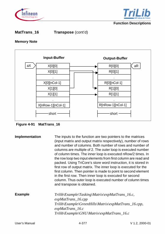
Function Descriptions
Memory Note
Figure 4-91 MatTrans_16
Implementation The inputs to the function are two pointers to the matrices (input matrix and output matrix respectively), number of rows and number of columns. Both number of rows and number of columns are multiple of 2. The outer loop is executed number of column times. The inner loop is executed nRow/2 times. In the row loop two input elements from first column are read and packed. Using TriCore’s store word instruction, it is stored in first row of output matrix. The inner loop is executed for the first column. Then pointer is made to point to second element in the first row. Then inner loop is executed for second column. Thus outer loop is executed number of column times and transpose is obtained.
Example Trilib\Example\Tasking\Matrix\expMatTrans_16.c, expMatTrans_16.cppTrilib\Example\GreenHills\Matrix\expMatTrans_16.cpp, expMatTrans_16.cTrilib\Example\GNU\Matrix\expMatTrans_16.c
MatTrans_16 Transpose (cont’d)
aX
X[0][1]
.
X[0][nCol-1]
X[1][0]
X[1][1]
.
X[0][0]
X[nRow-1][nCol-1]
aR
R[0][1]
.
R[0][nCol-1]
R[1][0]
R[1][1]
.
R[0][0]
R[nRow-1][nCol-1]
short short
Input-Buffer Output-Buffer
User’s Manual 4-377 V 1.2, 2000-01

Function Descriptions
Cycle Count For all X[nRow][nCol]
:
Code Size 52 bytes
MatTrans_16 Transpose (cont’d)
3nRow
2--------------- 5× 2 5+ + nCol×+
+2+2
User’s Manual 4-378 V 1.2, 2000-01

Function Descriptions
4.14 Statistical Functions
4.14.1 Descriptions
The following Statistical functions are described.
• Autocorrelation• Convolution• Mean Value
Autocorrelation
Correlation determines the degree of similarity between two signals. If two signals areidentical their correlation coefficient is 1, and if they are completely different it is 0. If thephase shift between them is 180 and otherwise they are identical, then correlationcoefficient is -1.
There are two types of correlation Cross Correlation and Autocorrelation.
When two independent signals are compared, the procedure is cross correlation. Whenthe same signal is compared to phase shifted copies of itself, the procedure isautocorrelation. Autocorrelation is used to extract the fundamental frequency of a signal.The distance between correlation peaks is the fundamental period of the signal. Discretecorrelation is simply a vector dot product.
[4.162]
where,
N = nX - j -1 (j = 0, 1,...,nR-1),
nX = Size of input vector
nR = Desired number of outputs. It can take values from 1 to nX
Autocorrelation is given by
(j = 0, 1,...,nR-1) [4.163]
i is the index of the array, j is the lag value, as it indicates the shift/lag considered for theR(j) autocorrelation. N is the correlation length and it determines how much data is usedfor each correlation result. When R(j) is calculated for a number of j values, it is referredto as autocorrelation function.
R j( ) x i( ) y i j+( )×
i 0=
N
∑=
R j( ) x i( ) x i j+( )×
i 0=
N
∑=
User’s Manual 4-379 V 1.2, 2000-01

Function Descriptions
Convolution
Discrete convolution is a process, whose input is two sequences, that provide a singleoutput sequence.
Convolution of two time domain sequences results in a time domain sequence. Samething applies to frequency domain.
Both the input sequences should be in the same domain but the length of the two inputsequences need not be the same.
Convolution of two sequences X(k) and H(k) of length nX and nH respectively can begiven mathematically as
[4.164]
The resulting output sequence R(n) is of length nX+nH-1.
The convolution in time domain is multiplication in frequency domain and vice versa.
R n( ) H k( ) X n k–( )⋅
k 0=
nX nH 2–+
∑=
User’s Manual 4-380 V 1.2, 2000-01

Function Descriptions
ACorr_16 Autocorrelation
Signature void ACorr_16( DataS *X, DataL *R, int nX, int nR );
Inputs XR
nXnR
::
::
Pointer to Input-VectorPointer to Output-Vector containing the first nR elements of the positive side of the autocorrelation function of the vector XSize of vector XSize of vector R
Output R : Output-Vector
Return None
Description The function performs the positive side of the autocorrelation function of real vector X. The arguments to the function are pointer to the input vector, pointer to output buffer to store autocorrelation result, size of input buffer (only even) and number of auto correlated outputs desired. The input values are in 16 bit fractional format and output values are in 32 bit fractional format. The implementation is optimal and works if size of output buffer is even/odd.
User’s Manual 4-381 V 1.2, 2000-01

Function Descriptions
Pseudo code
{ frac16 *X1; //Ptr to input vector frac16 *X2; //Ptr to input vector + LagCount frac64 acc; //Autocorrelation result int dCnt; //Correlation loop count //Macro macro ACorr; { int aCorlen; //Correlation loop count aCorlen = dCnt; //Correlation loop count for current autocorrelation //output for(i=0; i<aCorlen; i++) { acc = acc + *(X1++) * *(X2++) + *(X1++) * *(X2++); //acc = acc + X(0) * X(0+aLagCnt) + X(1) * //X(1+aLagCnt)(even correlation length) (or) //acc = acc + X(1) * X(1+aLagCnt) + X(2) * X(2+aLagCnt) //(odd correlation length) } } ACorr_16: { int lflag = 0; int aLagCnt = 0;//First autocorrelation output is with zero lag int dCnt = nX/2; X1 = X; //Initialize first Ptr to start of input vector if (nR%2 != 0) { nR++; lflag = 1; //lflag = 1 if nR is odd } //If desired no. of output is 1 or 2 skip ACorr_OutDataL if (nR == 2) go to ACorr_R_1or2; //ACorr_OutDataL for (i=0; i<nR/2-1; i++) { acc = 0; //Clear accumulator X2 = X + aLagCnt; //Second Ptr initialized to first Ptr plus an offset
ACorr_16 Autocorrelation (cont’d)
User’s Manual 4-382 V 1.2, 2000-01

Function Descriptions
//of aLagCnt ACorr; //Autocorrelation computation *R++ = (frac32_sat) acc; //Autocorrelation result converted to 32 bits with //saturation and stored to output buffer acc = 0; //Clear accumulator aLagCnt = aLagCnt + 2; //Lag count is incremented for the next correlation X1 = X; //Initialize first Ptr to start of input vector X2 = X2 + alagCnt; //Second Ptr initialized to first Ptr plus an offset //of aLagCnt
//Autocorrelation computation dCnt--; acc = acc + *(X1++) * *(X2++); //acc = acc + X(0) * X(0+aLagCnt) ACorr; X1 = X; //Initialize first Ptr to start of input vector aLagCnt = aLagCnt + 1; //Lag cnt incremented for next autocorrelation //computation }
//Last two results (if nR is even) or last one result (if nR is //odd) is calculated outside the loop ACorr_R_1or2: acc = 0; //Clear accumulator X2 = X + aLagCnt; ACorr; *R++ = (frac32_sat)acc; if (lflag == 1) //Jump to ACorr_16_Ret if lflag = 1 go to ACorr_Ret; else acc = 0; //Clear accumulator X1 = X; //Initialize first Ptr to start of input vector X2 = X2 + aLagCnt; acc = acc + *(X1++) * *(X2++); //If nR = nX, jump to ACorr_Rlast if (dCnt = 0) go to ACorr_Rlast; else
ACorr_16 Autocorrelation (cont’d)
User’s Manual 4-383 V 1.2, 2000-01

Function Descriptions
{ dCnt--; ACorr; } ACorr_Rlast: (*R++)(frac32_sat)acc; ACorr_Ret: }}
Techniques • Loop unrolling is done so that implementation is efficient forboth even and odd number of desired outputs. Last twooutputs (for nR even) or last one output (for nR odd) iscomputed outside the loop
• A macro ACorr is used to calculate each autocorrelationoutput. The macro uses packed load and dual MAC toreduce the number of cycles for a given correlation length
• One pass through the loop calculates two outputs, i.e.,there are two calls to the macro
• For odd correlation length one multiplication is performedbefore calling the macro
• Implementation is optimal for both even and odd values ofnR
• Intermediate result stored in 64 bit register (16 guard bits)• Instruction ordering for zero overhead Load/Store
Assumptions • Input is in 1Q15 format• Output is in 1Q31 format
ACorr_16 Autocorrelation (cont’d)
User’s Manual 4-384 V 1.2, 2000-01

Function Descriptions
Memory Note
Figure 4-92 ACorr_16
ACorr_16 Autocorrelation (cont’d)
Input-Vector
aX1
1Q15
X(1)
X(2)
.
X(n-1)
X(n)
X(n+1)
X(0)
.
aX
aX2 = aX1 + lag count
aX2
Dual MAC(even
Corr.len)
MAC (oddCorr.len)
halfwordaligned
Dual MAC(odd
Corr.len)
Output-Vector
aRR(1)
R(2)
.
.
.
.
R(0)
R(nR-1)
1Q31
halfwordaligned
User’s Manual 4-385 V 1.2, 2000-01

Function Descriptions
Implementation Correlation is similar to FIR filtering without the time reversal of the second input variable. In autocorrelation, the signal is multiplied with phase shifted copies of itself. The implementation begins with zero lag, i.e., the value at each instant is squared and added to produce the first autocorrelation output.
The lag value is incremented by one for each next output. Hence, in autocorrelation computation the number of multiplication (correlation length) needed for each R(i) decreases as i increases from 1 to nR-1. Since the given assumption is that the number of input is always even, correlation length is even for all R(j) where j = 0, 2, 4,....,nR-2 and it is odd when j = 1, 3, 5,...,nR-1. For each autocorrelation output computation, two pointers to input buffer aX1, aX2 are initialized such that aX1 points to beginning of input vector and the difference between them is equal to the lag value for that output, i.e., aX2 = aX1+lag count.
A macro ACorr is used to calculate each autocorrelation output. The macro uses packed load and dual MAC to reduce the number of cycles for a given correlation length. This brings down the loop count for each autocorrelation by a factor of 2. For all R(i), i = 0, 2, 4,...., the call to ACorr will directly give the autocorrelation result in a 64 bit register which is then converted with saturation to 1Q31 format and stored to output buffer. In case of R(i) with i = 1, 3, 5,..., the correlation length is odd. Hence, one MAC is performed before calling the ACorr macro. This makes the implementation optimal for all R(i). The loop in the ACorr_16 function runs (nR/2-1) times. During each pass through the loop two outputs are calculated and written to output buffer (there are two calls to ACorr). The implementation works for both odd and even values of nR, i.e., nR = 1, 2,...,nX.
ACorr_16 Autocorrelation (cont’d)
User’s Manual 4-386 V 1.2, 2000-01

Function Descriptions
Example Trilib\Example\Tasking\Statistical\expACorr_16.c, expACorr_16.cppTrilib\Example\GreenHills\Statistical\expACorr_16.cpp, expACorr_16.cTrilib\Example\GNU\Statistical\expACorr_16.c
Cycle Count For Macro ACorr
i = 2, 3,...,nX-2
i = 2, 3,...,nX-2
i = nX-1
where Mcall(i) refers to the ith call to the macro
For ACorr_16
a) When nR = any Even value less than nX and greater than 2
Pre-loop : 9
Loop :
Post-loop :
Example : When nX = 54, nR = 4
: Cycle Count = 274 cycles
b) When nR = any Odd value less than nX and greater than 1
Pre-loop : 9
Loop :
Post-loop :
ACorr_16 Autocorrelation (cont’d)
Mcall 1( ) 1 nX 2+ +=
Mcall i( ) 1 2 nX( ) 2⁄ i imod2–( ) 2⁄–( ) 2+×+=
Mcall i( ) 1 2 nX( ) 2⁄ i imod2–( ) 1⁄–( ) 2+×+=
Mcall i( ) 1 2 nX( ) 2⁄ i imod2–( ) 1⁄–( ) 2+×+=
19 nR 2⁄ 1–( ) Mcall 1( )+× …Mcall nR 2–( )
++
2 2 Mcall nR 1–( ) 14Mcall nR( ) 6 2
+ + + ++ +
19 nR 1+( ) 2⁄ 1–( ) ) Mcall 1( )+×… Mcall nR 1–( )
++
2 2 Mcall nR( ) 9 2+ + + +
User’s Manual 4-387 V 1.2, 2000-01

Function Descriptions
Example : When nX = 54, nR = 5
: Cycle Count = 335 cycles
c) When nR = nX
Pre-loop : 9
Loop :
Post-loop :
Example : When nR = nX = 54
: Cycle Count = 2141 cycles
d) When nR = 1
The OutData loop is bypassed
Cycle Count :
Example : When nX = 54, nR = 1
: Cycle Count = 79 cycles
e) When nR = 2
The OutData loop is bypassed
Cycle Count :
Example : When nX = 54, nR = 2
: Cycle Count = 145 cycles
Code Size 268 bytes
ACorr_16 Autocorrelation (cont’d)
19 nR 2⁄ 1–( ) Mcall 1( )+× …Mcall nX 2–( )
++
2 2 Mcall nX 1–( ) 17 2+ + + +
13 Mcall 1( ) 9 2+ + +
13 Mcall 1( ) 14 Mcall 2( )6 2+ + +
+ +
User’s Manual 4-388 V 1.2, 2000-01

Function Descriptions
Conv_16 Convolution
Signature void Conv_16(DataS *X, DataS *H, DataL *R, int nR, int nH );
Inputs XHRnHnR
:::::
Pointer to First Input-VectorPointer to Second Input-VectorPointer to Output-VectorSize of Second Input-VectorSize of Output-Vector
Output R(nR) : Output-Vector
Return None
Description The convolution of two sequences X and Y is done. The input vectors are 16-bit and returned output is 32-bit. All the vectors are halfword aligned. The length of input vectors is even. Therefore for full convolution length output vector length is always odd.
User’s Manual 4-389 V 1.2, 2000-01

Function Descriptions
Pseudo code
{ frac16 *X; //Ptr to First Input-Vector frac16 *H; //Ptr to Second Input-Vector frac64 acc; //Convolution result int dCnt; //Convolution loop count
//Macro macro Conv; { int aOvlpCnt; //Convolution loop count aOvlpCnt = dCnt;//Convolution loop count for current convolution //output
for(i=0; i<aOvlpCnt; i++) { acc = acc + (*(X-K)) (*) H(K) + (*(X-K-1)) (*) H(K+1) //acc += X(n) * H(0) + X(n-1) * H(i) K = K + 2; } Conv_16: { int anHCnt; int anX_nHCnt; int anR_nXCnt; int dCnt = 1; int nX_1;
dnHCnt = nH/2 - 1; anHCnt = dnHCnt; X1 = X; //Store Ptr to First Input-Vector H1 = H; //Store Ptr to Second Input-Vector *R++ = X[0].H[0] acc = 0.0; Conv; //Convolution computation *R++ = (frac32 sat)acc; //Result stored X1 = X1 + 2; X = X1; H = H1;
Conv_16 Convolution (cont’d)
User’s Manual 4-390 V 1.2, 2000-01

Function Descriptions
if (nR == 3) go to Conv_R_3; for (i=0; i<anHCnt; i++) { acc = 0.0; acc = X[n] (*) H[0]; Conv; //Convolution computation *R++ = (frac16 sat)acc; //Result stored dCnt++; X = X1; H = H1; acc = 0.0; Conv; //Convolution computation X1 = X1 + 2; X = X1; H = H1; *R++ = (frac32 sat)acc; } nX_1 = nR - nH; X1 = X1 - 1; X = X1; anR_nXCnt = dnHCnt; if (nX == nH) go to Conv_DCntr;
H = H1; anX_nHCnt = nX - nH; for (i=0; i<anX_nHCnt; i++) { X = X1; acc = 0.0; Conv; //Convolution computation X1 = X1 + 1; H = H1; *R++ = (frac32 sat)acc; //Result stored }
Conv_16 Convolution (cont’d)
User’s Manual 4-391 V 1.2, 2000-01

Function Descriptions
X = X1; for (i=0; i<anR_nXCnt; i++) { dCnt--; H1 = H1 + 1; H = H1; acc = 0.0; acc = X(n) (*) H(0); Conv; //Convolution computation *R++ = (frac32 sat)acc; X1 = X1 - 1; H1 = H1 + 1; X = X1; H = H1; acc = 0.0; Conv; //Convolution computation *R++ = (frac32 sat)acc; X1 = X1 + 1; X = X1; }
Conv_R_3; acc = 0.0; acc = X(nX - 1) (*) H(nH - 1); K++ = (frac32)acc;
return; }}
Techniques • For optimization implementation is divided into three loops.First loop where overlap count increases, second loopoverlap count remains same and third loop overlap countdecreases
• A macro Conv is used which calculates convolution output.The macro uses packed load and dual MAC to reduce thenumber of cycles for a given overlap count of twosequences
• Use of dual MAC and MAC instructions• Intermediate results stored in 64 bit register (16 guard bits)• Instruction ordering for zero overhead Load/Store
Assumptions • Inputs are in 1Q15 format, Output is in 1Q31 format• nX and nH are even and hence nR is always odd
Conv_16 Convolution (cont’d)
User’s Manual 4-392 V 1.2, 2000-01

Function Descriptions
Memory Note
Figure 4-93 Conv_16
Conv_16 Convolution (cont’d)
First Input-Vector Second Input-Vector
aH
H(1)
H(2)
.
.
.
.
H(0)
H(nH-1)
.
X(n-2)
X(n-1)
X(n)
.
.
X(0)
X(nR-nH)
halfwordaligned
halfwordaligned
1Q151Q15 MAC(odd
overlapcount)
Dual MAC(even
overlapcount)
aX1
Dual MAC(odd
overlapcount)
Output-Vector
aRR(1)
R(2)
.
.
.
.
R(0)
R(nR-1)
1Q31
halfwordaligned
User’s Manual 4-393 V 1.2, 2000-01

Function Descriptions
Implementation Convolution is same as FIR filtering. For convolution one of the two sequences is inverted in time. To implement the convolution, the two sequences are multiplied together and the products are summed to compute the output sample. To calculate next output sample time inverted signal is shifted by one and process is repeated. If two sequences of length nX and nH are convolved the convolution length is given by nR = nX+nH-1.
The pointer to input vectors, output vector, the size of output vector (nR) and size of the input sequence of smaller length (nH) are sent as arguments. The size of the other input sequence is calculated as (nR-nH+1).
Implementation uses macro Conv. The macro uses two load word and one dual MAC instruction. Thus two multiplications and one addition is performed per loop according to the equation
[4.165]
Thus loop count is always (overlap count/2-2) for even andodd lengths of overlap count. For odd one more MAC isperformed before the macro is called.
The convolution is divided into three loops.
First loop: The first two convolution outputs are given as
[4.166]
[4.167]
The number of multiplication and additions required forcomputation of R(i) increases as i is increased from 0 to nH-1. The overlap count of the two input sequences is even for i= 1, 3, 5,...,nH-1 and odd for i = 0, 2, 4,...,nH-2. Macro is calledfor every R(n).
Conv_16 Convolution (cont’d)
acc acc X n( ) H 0( )⋅ X n 1–( ) H 1( )⋅+ +=
R 0( ) X 0( ) H 0( )⋅=
R 1( ) X 1( ) H 0( )⋅ X 0( ) H 1( )⋅+=
User’s Manual 4-394 V 1.2, 2000-01

Function Descriptions
The first loop is unrolled and first two outputs are calculatedoutside the loop. One pass through the first loop gives twooutputs. Thus loop count for first loop is (nH/2-2). This loopgives first nH outputs.
Second loop: Here the overlap count is always constant andis nH. Macro Conv is called for (nX-nH) times. This loop givesnext (nX-nH) outputs.
This loop is skipped if nX = nH.
Third loop: The overlap count decreases from (nH-1) to 1 as iincreases from (nX+1) to (nR-1). The loop is unrolled and lastoutput which needs only one multiplication is done outside theloop. Thus loop count for this loop is (nH/2-2).
Example Trilib\Example\Tasking\Statistical\expConv_16.c, expConv_16.cppTrilib\Example\GreenHills\Statistical\expConv_16.cpp, expConv_16.cTrilib\Example\GNU\Statistical\expConv_16.c
Cycle Count For i = 1 to nH-1
Mcall(1) and Mcall(2) = 1+2+1
for i = 3, 5,...,(nH-1)
for i = 4,...,(nH-2)
For i = nH to nX-1
for i = nH,nH+1,...,(nX-1)
For i = nX to nR-2
Conv_16 Convolution (cont’d)
Mcall i( ) 1 2 i 1+( ) 2⁄ 2+×+=
Mcall i( ) 1 2 i 2⁄ 2+×+=
Mcall i( ) 1 2 nH 2⁄ 2+×+=
User’s Manual 4-395 V 1.2, 2000-01

Function Descriptions
for i = nX, nX+2,...,(nR-5)
for i = nX+1, nX+3,...,(nR-4)
Mcall(nR-3) and Mcall(nR-2) = 1+2+1
For nX>nH
14+Mcall(1)
First loop
For nH>4
For nH = 4
Second loop
Third loop
2+2
For nX = nH
Second loop is skipped and first loop will take 2 extra cyclesfor jump
For nH = nX =2
16+Mcall(1)+4
Code Size 420 bytes
Conv_16 Convolution (cont’d)
Mcall i )( ) 1 2 nH 2⁄ i 2⁄ nX( ) 2⁄– 1+( )–( ) 2+×+=
Mcall i )( ) 1 2 nH 2⁄ i 1–( ) 2⁄ nX( ) 2⁄– 1+( )–( ) 2+×+=
nH 2⁄ 1–( ) 18 Mcall 2( ) Mcall 3( ) … Mcall nH 1–( )+ + + +[ ]8+
nH 2⁄ 1–( ) 18 Mcall 2( ) Mcall 3( ) … Mcall nH 1–( )+ + + +[ ]7+
nX nH–( ) 8 Mcall nH( ) Mcall nH 1+( ) …Mcall nX 1–( )
+ + + +[] 3+
nH 2⁄ 1–( ) 19 Mcall nX( ) Mcall nX 1+( ) …Mcall nR 2–( )
+ + + +[] 2+
User’s Manual 4-396 V 1.2, 2000-01

Function Descriptions
Avg_16 Mean Value
Signature DataS Avg_16(DataS *X, int nX );
Inputs XnX
::
Pointer to Input-BufferSize of Input-Buffer
Output None
Return R : Mean value of the input values
Description This function calculates the mean of a given array of values. It takes pointer to the array and size of the array as input. Input range is [-1, 1). The return is the mean value represented using 32 bits.
Pseudo code
{ frac32 acc = 0; //Sum of inputs frac32 one_nX; //1/no. Of inputs frac64 Ra; frac32 R;
for(i=0; i<nx; i++) { acc = acc + X[i]; //acc in 17Q15 format } one_nX = 1/nX; //one_nX in 1Q31 format Ra = acc (*) one_nX; //Mean value in 17Q47 format R = (frac32)Ra; //32 bit result in 1Q31 format }
Techniques • 32 bit addition is used to provide 16 guard bits for addition • Instruction ordering provided for zero overhead Load/Store
Assumptions • Inputs are in the range [-1,1) and in 1Q15 format. Output isalso in 1Q15 format.
User’s Manual 4-397 V 1.2, 2000-01

Function Descriptions
Memory Note
Figure 4-94 Avg_16
Implementation The function takes a short pointer to an array whose mean is to be calculated and the size of the array as input. The return value is the 32 bit mean value.
[4.168]
Load of inputs and addition are performed in a loop. The input values are read into the lower 16 bits of a 32 bit register. Hence 32 bit addition is performed on 17Q15 values thereby providing 16 guard bits for addition. The reciprocal of the size is calculated.The product of the sum and the reciprocal gives the mean value in 17Q47 format. This is converted to 1Q31 and returned.
Avg_16 Mean Value (cont’d)
aX
X(1).
.
.
.
.
X(0)
X(nX-1)
Input-Buffer
1Q15
meanx 0( ) x 1( ) … x nx 1–( )+ + +
nx-----------------------------------------------------------------------=
User’s Manual 4-398 V 1.2, 2000-01

Function Descriptions
Example Trilib\Example\Tasking\Statistical\expAvg_16.c, expAvg_16.cppTrilib\Example\GreenHills\Statistical\expAvg_16.cpp, expAvg_16.cTrilib\Example\GNU\Statistical\expAvg_16.c
Cycle Count Pre-loop : 3
Loop :
Post-loop : 27+2
Code Size 54 bytes
Avg_16 Mean Value (cont’d)
nX 2+
User’s Manual 4-399 V 1.2, 2000-01

Function Descriptions
User’s Manual 4-400 V 1.2, 2000-01

Applications
5 ApplicationsThe following applications are described.
• Spectrum Analyzer• Sweep Oscillator• Equalizer
5.1 Spectrum Analyzer
To perform a spectral analysis of any signal spectrum analyzer is used. The spectrumanalyzer uses radix-2 FFT to get the frequency content of a signal. The FFT algorithmtakes N-data-samples x(n), n=0,1,...,N-1 of the input given and produces N-pointcomplex frequency samples X(K), K=0,1,...,N-1. The power spectrum is obtained bysquaring the scaled magnitude of complex frequency samples.
K=0,1,...,N/2 [5.1]
The Power Spectrum Density (PSD) gives a measure of the distribution of the averagepower of a signal over frequency.
The PSD can be actual or averaged. The actual PSD gives N/2 point output from N pointcomplex FFT output. The averaged PSD gives b band output where the number of bandsis user input.
A simple example showing functioning of Spectrum Analyzer.
The following are the diagrams where input given is a mixture of 4kHz and 12kHz sinewaves sampled at 32kHz. The FIR filter has a cutoff frequency of 8 kHz. So after filteringthe input to FFT contains only 4kHz wave. The power spectrum gives the correspondingfrequency. Here the number of FFT points taken is 512. The maximum frequency valuerepresented by the spectrum is 16K as sampling frequency is 32K. Since FFT is of 512complex points it will result in a power spectrum of 256 points. Here 256th doppler binrepresents frequency of 16K. So the frequency corresponding to 64th doppler bin is 4K.
P K( ) 1N---- X K( ) 2 1
N---- Re X K( )2[ ] Im X K( )2[ ]+{ }= =
User’s Manual 5-401 V 1.2, 2000-01

Applications
Figure 5-1 Input given to Spectrum Analyzer
Figure 5-2 Output of FIR filter
User’s Manual 5-402 V 1.2, 2000-01

Applications
Figure 5-3 Output power spectrum considering actual PSD
Figure 5-4 20 Band averaged power spectrum
User’s Manual 5-403 V 1.2, 2000-01

Applications
5.2 Sweep Oscillator
The generation of pure tones is often used for testing DSP systems and to synthesizewaveforms of required frequencies. The basic oscillator is a special case of an IIR filterwhere the poles are on the unit circle and the initial conditions are such that the input isan impulse. If the poles are moved outside the unit circle, the oscillator output will growat an exponential rate. If the poles are placed inside the unit circle, the output will decaytoward zero. The state (or history) of the second-order section determines the amplitudeand phase of the future output.
The impulse of a continuous second order oscillator is given by
[5.2]
If d>0 then the output will decay toward zero and the peak will occur at
[5.3]
The peak value will be
[5.4]
A second order difference can be used to generate an approximation response of thiscontinuous-time output. The equation for a second-order discrete time oscillators isbased on an IIR filter and is as follows
[5.5]
where, the x input is only present for t=0 as an initial condition to start the oscillator and
[5.6]
[5.7]
where, is the sampling period (1/fs) and is 2 times the oscillator frequency.
The frequency and rate of change of envelope of the oscillator output can be changedby modifying the values of d and on a sample by sample basis.
The sweep oscillator implemented here uses the function IirBiq_4_16.
When the oscillator has to be started, the function oscillator is called with one of thearguments indicating to start new oscillator where impulse is given as an input and the
R t( ) edt– ωtsin
ω--------------=
tpeakArc ω d⁄( )tan
ω----------------------------------=
R tpeak( ) edt– peak
d2 ω2
+----------------------=
Rn 1+ a1yn a2yn 1– b1xn+–=
a1 2edτ– ωτ( )cos=
a2 edτ–
=
τ ω π
ω
User’s Manual 5-404 V 1.2, 2000-01

Applications
delay line gets updated. From the next sample onwards input is made zero, but as thepoles lie on the unit circle the output is oscillatory at given frequency. The coefficients,whenever there is frequency change, are calculated for that particular frequency.
Following parameters are programmable
• The sampling frequency• Start frequency• The factor, by which frequency has to be incremented or decremented• The number of cycles for a start frequency• Number of cycles for changed frequency
Figure 5-5 Sweep Oscillator
User’s Manual 5-405 V 1.2, 2000-01

Applications
5.3 Equalizer
A Graphic Equalizer is a powerful tool to characterize and enhance audio signals.
Technically it is composed of a bank of band-pass filters, each with a fixed centerfrequency and a variable gain. This kind of processing unit is called Graphic since theposition of the slider resembles the frequency response of the filters bank. Thus itsusage is extremely intuitive, moving the slider up boosts a selected band, moving it downwill cut it.
Graphic equalizer uses high quality constant Q digital filters. This allows to isolate everyfilter section from the effects of the amplitude with respect to the centre frequency andbandwidth. The result is an accurate control permitting each band not to affect theadjacent ones.
5-band equalizer implemented uses 128-tap FIR filters to get the desired band pass filterresponse. Here the function FirBlk_16 is used for FIR filtering.
The five bands are
• 0 - 170• 170 - 600• 600 - 3K• 3K - 12K• 12K - 16K
The gain in dB for each band is programmable. Also the common master gain isprogrammable. The filters are designed for three sampling frequencies 32kHz, 44.1kHz,48kHz. The user gives the desired sampling frequency as an input. Depending on thiscorresponding filter bank is selected. After input is passed through all the five filters theoutput of each filter is multiplied with the gain for that particular band. All the outputs areadded and then finally multiplied with master gain to get the equalizer output.
User’s Manual 5-406 V 1.2, 2000-01

Applications
Figure 5-6 5 Band Graphic Equalizer
85 600 3K 12K170 16K14K
frequency
-3dB
0dB
7.5K1800385
User’s Manual 5-407 V 1.2, 2000-01

Applications
5.4 Hardware Setup for Applications
Figure 5-7 Hardware Setup
1. Preparing the TriBoard for Debugging
Connect a parallel cable from the parallel port on the PC to the On Board Wiggler (DB25)on the TriBoard as shown in Figure 5-7. Connect a “one to one” serial port cable fromthe RS232 interface on the PC to the serial interface (RS232-0) on the TriBoard. Fordetails refer TriBoard manual.
2. Starting a Terminal Program
A terminal program can be used to communicate with the TriBoard via RS232. Bothtransmit and receive of data is possible. The TriBoard has an RS232 transceiver onboard to meet the RS232 specification of your PC.
Power supply
Parallel port
Serial port
User’s Manual 5-408 V 1.2, 2000-01

Applications
3. Power Up the TriBoard
Connect the power supply (6V to 25V DC, power plug with surrounding ground) to the
lower left edge of the card as shown in Figure 5-7. Power up the unit. The green LED’snext to the OCDS2 Connector indicates the right power status. The red LED near
the reset button indicates the reset status.
Once the connections are done the applications can be run over the TriBoard. Thespectrum analyzer and the equalizer applications can be run by reading the input fromthe serial port of TriBoard and calculated output is sent again to serial port of TriBoard.
User’s Manual 5-409 V 1.2, 2000-01

Applications
5.4.1 Spectrum Analyzer
Frontend for Spectrum Analyzer:
Figure 5-8 Frontend of Spectrum Analyzer
Figure 5-9 Settings for Spectrum Analyzer
User’s Manual 5-410 V 1.2, 2000-01

Applications
Figure 5-10 Actual PSD of the input (128 point power spectrum)
Figure 5-11 Averaged PSD of the input (10 bands)
User’s Manual 5-411 V 1.2, 2000-01
Applications
The inputs taken from the user are
1. Actual band or average band2. Sampling frequency3. Cutoff frequency
Actual band gives 128 point power spectrum of the given 1024 input samples.
Sampling frequency can be one of the three choices 32K, 44.1K, and 48K.
Cutoff frequency can be one of the three choices 4K, 8K, and 16K.
From the host machine, first 1 byte is sent to the serial port of TriBoard to get the aboveuser inputs. Then acknowledgement is sent to host machine as 1 byte is received. Thenfollows the data from the host machine to the TriBoard. 1024, 16 bit data is sent to theTriBoard. This data is read in a buffer. The FFT of 1024 points input data is calculated.From the frequency spectrum, power spectrum density is calculated by squaring thescaled magnitude complex frequency samples. Then 128 point PSD is calculated from512 point PSD by averaging. If user input is actual PSD, the 128 point PSD is sent toserial port of TriBoard. If the user input is average input then calculated PSD is dividedinto 10 segments and averaged 10 bands are sent to serial port. The host machine readsthe data on the serial port and displays actual or averages spectrum depending on userinput.
User’s Manual 5-412 V 1.2, 2000-01

Applications
5.4.2 Equalizer
Frontend for Equalizer:
Settings:
Figure 5-12 Frontend of Equalizer
User’s Manual 5-413 V 1.2, 2000-01

Applications
Figure 5-13 Settings for Equalizer
The inputs taken from the user are
1. Sampling frequency2. 5 band gains in dB3. Master gain in dB
Sampling frequency can be one of the three choices 32K, 44.1K and 48K.
Band gains can be from -20dB to +20dB.
Master gain can be from 0 to +50dB.
User’s Manual 5-414 V 1.2, 2000-01
Applications
From the host machine, first 13 bytes are sent to the serial port of TriBoard to get theabove user inputs. Then a one byte acknowledgement is sent to the host machine. Thisis followed by the data from the host machine. 128, 16 bit data is sent to the TriBoard.This data is read in a buffer. This is band passed through 5 Band pass filters. Each ofthe outputs of the filters is multiplied by the respective gain and the final output isgenerated by their sum. This is then multiplied by the master gain and sent back to thehost machine. The host machine then sends this data to an output file.
User’s Manual 5-415 V 1.2, 2000-01

Applications
User’s Manual 5-416 V 1.2, 2000-01

References
6 References
1. Digital Signal Processing by Alan V Oppenheim and Ronald W Schafer2. Digital Signal Processing, A Practical Approach by Emmanuel C Ifeachor and Barrie
W Jervis3. Discrete-Time Signal Processing by Alan V Oppenheim and Ronald W Schafer4. Advanced Engineering Mathematics by Erwin Kreyszig5. K. R. Rao and P. Yip, Discrete Cosine Transform: Algorithms, Advantages,
Applications6. W. H. Chen, C. H. Smith, and S. C. Fralick, "A fast computational algorithm for the
Discrete Cosine Transform"
User’s Manual 6-417 V 1.2, 2000-01

References
User’s Manual 6-418 V 1.2, 2000-01

Frequently Asked Questions
7 Frequently Asked Questions
7.1 FIR Basics
1. What are FIR filters?
FIR filters are one of two primary types of digital filters used in Digital Signal Processing(DSP) applications (the other type being IIR). FIR means Finite Impulse Response.
2. Why is the impulse response "finite"?
The impulse response is "finite" because there is no feedback in the filter, if an impulseis given as an input (i.e., a single one sample followed by many zero samples), zeroeswill eventually come out after the one sample has made its way in the delay line past allthe coefficients.
3. What is the alternative to FIR filters?
DSP filters can also be Infinite Impulse Response (IIR). IIR filters use feedback, so whenan impulse is input the output theoretically rings indefinitely.
4. How do FIR filters compare to IIR filters?
Each has advantages and disadvantages. Overall, the advantages of FIR filtersoutweigh the disadvantages, so they are used much more than IIRs.
a) What are the advantages of FIR Filters as compared to IIR filters?
Compared to IIR filters, FIR filters have the following advantages.
• They can easily be designed to be "linear phase". Simple linear-phase filters delay theinput signal, but do not distort its phase.
• They are simple to implement. On most DSP microprocessors, the FIR calculation canbe done by looping a single instruction.
• They are suited to multi-rate applications. By multi-rate, we mean either decimation(reducing the sampling rate), interpolation (increasing the sampling rate) or both.Whether decimating or interpolating, the use of FIR filters allows some of thecalculations to be omitted, thus providing an important computational efficiency. Incontrast, if IIR filters are used, each output must be individually calculated, even if thatoutput is discarded. (so the feedback will be incorporated into the filter.)
• They have desirable numeric properties. In practice, all DSP filters must beimplemented using finite-precision arithmetic, i.e., a limited number of bits. The use offinite-precision arithmetic in IIR filters can cause significant problems due to the useof feedback, but FIR filters have no feedback, so they can usually be implementedusing fewer bits.
User’s Manual 7-419 V 1.2, 2000-01

Frequently Asked Questions
• They can be implemented using fractional arithmetic. Unlike IIR filters, it is alwayspossible to implement an FIR filter using coefficients with magnitude of less than 1.0.(The overall gain of the FIR filter can be adjusted at its output, if desired). This is animportant consideration when using fixed-point DSP's, because it makes theimplementation much simpler.
b) What are the disadvantages of FIR Filters as compared to IIR filters?
FIR filters sometimes have the disadvantage that they require more memory and/orcalculation to achieve a given filter response characteristic. Also, certain responses arenot practical to implement with FIR filters.
5. What terms are used in describing FIR filters?
Impulse Response - The impulse response of an FIR filter is actually just the set of FIRcoefficients. (If an impulse is put into an FIR filter which consists of a one samplefollowed by many zero samples, the output of the filter will be the set of coefficients, asthe one sample moves past each coefficient in turn to form the output.)
Tap - An FIR tap is simply a coefficient/delay pair. The number of FIR taps, (oftendesignated as N) is an indication of
• The amount of memory required to implement the filter • The number of calculations required• The amount of filtering the filter can do
In effect, more taps means more stopband attenuation, less ripple, narrower filters, etc.
7.1.1 FIR Properties
Linear Phase
1. What is the association between FIR filters and linear-phase?
Most FIRs are linear-phase filters. When a linear-phase filter is desired an FIR is usuallyused.
2. What is a linear phase filter?
Linear Phase refers to the condition where the phase response of the filter is a linear(straight-line) function of frequency (excluding phase wraps at +/- 180 degrees). Thisresults in the delay through the filter being the same at all frequencies. Therefore, thefilter does not cause phase distortion or delay distortion. The lack of phase/delaydistortion can be a critical advantage of FIR filters over IIR and analog filters in certainsystems, for example, in digital data modems.
User’s Manual 7-420 V 1.2, 2000-01

Frequently Asked Questions
3. What is the condition for linear phase?
FIR filters are usually designed to be linear-phase (but they don’t have to be). An FIRfilter is linear-phase if (and only if) its coefficients are symmetrical around the centercoefficient, i.e., the first coefficient is the same as the last, the second is the same as thenext-to-last, etc. (A linear-phase FIR filter having an odd number of coefficients will havea single coefficient in the center which has no mate.)
4. What is the delay of a linear-phase FIR?
The formula is simple. Given an FIR filter which has N taps, the delay is
(N - 1) / Fs, where Fs is the sampling frequency. So, for example, a 21 tap linear-phaseFIR filter operating at a 1 kHz rate has delay (21 - 1) / 1 kHz = 20 milliseconds.
Frequency Response
1. What is the Z transform of an FIR filter?
For an N-tap FIR filter with coefficients h(k), whose output is described by
[7.1]
The filter’s Z transform is
[7.2]
2. What is the frequency response formula for an FIR filter?
The variable z in H(z) is a continuous complex variable and can be described as
[7.3]
where,
r is the magnitude and w is the angle of z.
let r = 1, then H(z) around the unit circle becomes the filter’s frequency response H(ejw).This means that substituting ejw for z in H(z) gives an expression for the filter’s frequencyresponse H(ejw), which is
or [7.4]
Using Euler’s identity,
[7.5]
y n( ) h 0( ) x n( )⋅ h 1( ) x n 1–( )⋅ h 2( ) x n 2–( )⋅ … h N 1–( ) x n N– 1–( )⋅+ + + +=
H z( ) h 0( )z 0–h 1( )z 1–
h 2( )z 2– … h N 1–( )z N 1–( )–+ + + +=
z rejw
=
H ejw( ) h 0( )e j0w–
h 1( )e j1w–h 2( )e j2w– … h N 1–( )e j N 1–( )w–
+ + + +=
eja–
a( )cos j a( )sin–=
User’s Manual 7-421 V 1.2, 2000-01

Frequently Asked Questions
H(w) can be written in rectangular form as
[7.6]
3. How to scale the gain of an FIR filter?
Multiply all coefficients by the scale factor.
Numeric Properties
1. Are FIR filters inherently stable?
Yes, since they have no feedback elements, any bounded input results in a boundedoutput.
2. What makes the numerical properties of FIR filters good?
The key is the lack of feedback. The numeric errors that occur when implementing FIRfilters in computer arithmetic occur separately with each calculation, the FIR does notremember its past numeric errors. In contrast, the feedback aspect of IIR filters cancause numeric errors to compound with each calculation, as numeric errors are fed back.The practical impact of this is that FIRs can generally be implemented using fewer bitsof precision than IIRs. For example, FIRs can usually be implemented with 16-bits, butIIRs generally require 32-bits, or even more.
6. Why are FIR filters generally preferred over IIR filters in multirate (decimating andinterpolating) systems?
Because only a fraction of the calculations that would be required to implement adecimating or interpolating FIR in a literal way actually needs to be done.
Since FIR filters do not use feedback, only those outputs which are actually going to beused have to be calculated. Therefore, in case of decimating FIRs (in which only 1 of Noutputs will be used), the other N-1 outputs do not have to be calculated. Similarly, forinterpolating filters (in which zeroes are inserted between the input samples to raise thesampling rate) the inserted zeroes need not have to be multiplied with theircorresponding FIR coefficients and sum the result, the multiplication-additions that areassociated with the zeroes are just omitted. (because they don’t change the resultanyway.)
In contrast, since IIR filters use feedback, every input must be used, and every inputmust be calculated because all inputs and outputs contribute to the feedback in the filter.
H jw( ) h 0( ) 0w( )cos j 0w( )sin–[ ] h 1( ) 1w( )cos j 1w( )sin–[ ] …+ +=
+ h N 1–( ) N 1–( )w( )cos j N 1–( )w( )sin–[ ]
User’s Manual 7-422 V 1.2, 2000-01

Frequently Asked Questions
7.1.2 FIR Design
1. What are the methods of designing FIR filters?
The three most popular design methods are (in order):
a) Parks-McClellan: The Parks-McClellan method is probably the most widely usedFIR filter design method. It is an iteration algorithm that accepts filter specificationsin terms of passband and stopband frequencies, passband ripple, and stopbandattenuation. The fact that all the important filter parameters can be directly specifiedis what makes this method so popular. The Parks-McClellan method can design notonly FIR filters but also FIR differentiators and FIR Hilbert transformers.
b) Windowing: In the windowing method, an initial impulse response is derived bytaking the Inverse Discrete Fourier Transform (IDFT) of the desired frequencyresponse. Then, the impulse response is refined by applying a data window to it.
c) Direct Calculation: The impulse responses of certain types of FIR filters (e.g.Raised Cosine and Windowed Sine) can be calculated directly from formulae.
User’s Manual 7-423 V 1.2, 2000-01

Frequently Asked Questions
7.2 IIR Basics
1. What are IIR filters?
IIR filters are one of two primary types of digital filters used in Digital Signal Processing
(DSP) applications (the other type being FIR). IIR means Infinite Impulse Response.
2. Why is the impulse response "infinite"?
The impulse response is "infinite" because there is feedback in the filter, if an impulse isgiven as an input (a single 1 sample followed by many 0 samples), an infinite number ofnon-zero values will come out (theoretically).
3. What is the alternative to IIR filters?
DSP filters can also be Finite Impulse Response (FIR). FIR filters do not use feedback.
So, for an FIR filter with N coefficients, the output always becomes zero after putting in N
samples of an impulse response.
4. What are the advantages of IIR filters as compared to FIR filters?
IIR filters can achieve a given filtering characteristic using less memory and fewercalculations than a similar FIR filter.
5. What are the disadvantages of IIR filters as compared to FIR filters? • They are more susceptible to problems of finite-length arithmetic, such as noise
generated by calculations and limit cycles. (This is a direct consequence offeedback, when the output is not computed perfectly and is fed back, the imperfectioncan compound.)
• They are harder (slower) to implement using fixed-point arithmetic. • They do not offer the computational advantages of FIR filters for multirate
(decimation and interpolation) applications.
User’s Manual 7-424 V 1.2, 2000-01

Frequently Asked Questions
7.3 FFT
The Fast Fourier Transform is one of the most important topics in Digital SignalProcessing but it is a confusing subject which frequently raises questions. Here, weanswer Frequently Asked Questions (FAQs) about the FFT.
7.3.1 FFT Basics
1. What is FFT?
The Fast Fourier Transform (FFT) is a fast (computationally efficient) way to calculatethe Discrete Fourier Transform (DFT).
2. How does the FFT work?
By making use of periodicities in the sines that are multiplied to do the transforms, theFFT greatly reduces the amount of calculation required.
Functionally, the FFT decomposes the set of data to be transformed into a series ofsmaller data sets to be transformed. Then, it decomposes those smaller sets into evensmaller sets. At each stage of processing, the results of the previous stage are combinedin special way. Finally, it calculates the DFT of each small data set. For example, an FFTof size 32 is broken into 2 FFTs of size 16, which are broken into 4 FFTs of size 8,which are broken into 8 FFTs of size 4, which are broken into 16 FFTs of size 2.Calculating a DFT of size 2 is trivial.
This can be explained as follows. It is possible to take the DFT of the first N/2 points andcombine them in a special way with the DFT of the second N/2 points to produce a singleN-point DFT. Each of these N/2-point DFTs can be calculated using smaller DFTs in thesame way. One (radix-2) FFT begins, therefore, by calculating N/2 2-point DFTs. Theseare combined to form N/4 4-point DFTs. The next stage produces N/8 8-point DFTs andso on, until a single N-point DFT is produced.
3. How efficient is the FFT?
The DFT takes N2 operations for N points. Since at any stage the computation requiredto combine smaller DFTs into larger DFTs is proportional to N and there are log2(N)stages (for radix-2), the total computation is proportional to N * log2(N). Therefore, theratio between a DFT computation and an FFT computation for the same N isproportional to N / log2(n). In cases where N is small this ratio is not very significant, butwhen N becomes large, this ratio gets very large. (Every time N is doubled, thenumerator doubles, but the denominator only increases by 1.)
4. Are FFTs limited to sizes that are powers of 2?
User’s Manual 7-425 V 1.2, 2000-01

Frequently Asked Questions
No. The most common and familiar FFTs are radix-2. However, other radices aresometimes used, which are usually small numbers less than 10. For example, radix-4 isespecially attractive because the twiddle factors are all 1, -1, j or -j, which can beapplied without any multiplications at all.
Also, mixed radix FFTs can be done on composite sizes. In this case, you break a non-prime size down into its prime factors and do an FFT whose stages use those factors.For example, an FFT of size 1000 might be done in six stages using radices of 2 and 5,since 1000 = 2 * 2 * 2 * 5 * 5 * 5. It can also be done in three stages using radix-10, since1000 = 10 * 10 * 10.
5. Can FFTs be done on prime sizes?
Yes, although these are less efficient than single-radix or mixed-radix FFTs. It is almostalways possible to avoid using prime sizes.
7.3.2 FFT Terminology
1. What is an FFT radix?
The radix is the size of an FFT decomposition. For single-radix FFTs, the transform sizemust be a power of the radix.
2. What are twiddle factors?
Twiddle factors are the coefficients used to combine results from a previous stage toform inputs to the next stage.
3. What is an "in place" FFT?
An "in place" FFT is an FFT that is calculated entirely inside its original samplememory. In other words, calculating an "in place" FFT does not require additional buffermemory. (as some FFTs do.)
4. What is bit reversal?
Bit reversal is just what it sounds like, reversing the bits in a binary word from left toright. Therefore the MSB’s become LSB’s and the LSB’s become MSB’s. The dataordering required by radix-2 FFTs turns out to be in bit reversed order, so bit-reversedindices are used to combine FFT stages. It is possible (but slow) to calculate these bit-reversed indices in software. However, bit reversals are trivial when implemented inhardware. Therefore, almost all DSP processors include a hardware bit-reversalindexing capability. (which is one of the things that distinguishes them from othermicroprocessors.)
User’s Manual 7-426 V 1.2, 2000-01

Frequently Asked Questions
5. What is decimation in time versus decimation in frequency?
FFTs can be decomposed using DFTs of even and odd points, which is called aDecimation-In-Time (DIT) FFT or they can be decomposed using a first-half/second-halfapproach, which is called a Decimation-In-Frequency (DIF) FFT.
User’s Manual 7-427 V 1.2, 2000-01

Frequently Asked Questions
User’s Manual 7-428 V 1.2, 2000-01

Appendix
8 Appendix
Convention Document for TriLib
8.1 Introduction
8.1.1 Scope of the Document
This document describes the Programming Conventions for the TriCore DSP Library.
The purpose of the document is to bring out a unified programming style for the TriCoreDSP. It is recommended that the guidelines and the conventions be observed toorganize each DSP application software. This ensures uniform and well-structured code.
User’s Manual 8-429 V 1.2, 2000-01

Appendix
8.2 File Organization
8.2.1 File Extensions
The Software application, TriLib should be organized as a collection of modules or filesthat belongs to any one of the following categories. The following table brings out thedetails of the different categories of files.
Table 8-1 Directory Structure
Type Extension Description
’C’ Source files *.c C Language Source files
Include files *.h, *.inc The include files for the ’C’ and the assembly functions. The C include files generally have *.h as extension. Assembly can have different extensions based on the compiler in use. All the include files should define the global constants and variable types, if any. They should not allocate memory or define functions as this prevents them from being included by multiple source files. All subroutines which form part of the overall interface to a source file should be declared in include file. This provides a convenient overview of the interface and allows the compiler or assembler to check for errors
Testvector files *.dat These files should only contain data to be used for test purposes or algorithmic usage. There must not be any code in these data files. These files, if used, will probably be included or copied (.include directive) in other source files or assembled as stand-alone modules. These files can also be given as the command line argument for the example programs depending upon the implementation
Build files *.pjt, *.bld, *.out It is strongly recommended that a project make fileis maintained that checks for any out-of-date targetfiles and builds them automatically. Differentcompilers use different extension for the build files.
TriCore Source files
*.asm, *.tri, *.S Different compilers use different extensions for theassembly source files. Generally *.asm file is widelyaccepted by many compilers.
User’s Manual 8-430 V 1.2, 2000-01

Appendix
8.2.2 File Naming Conventions
The Files will be named using the following convention. This helps in easy identificationof the file.
• All the Source files of TriCore assembly will have *.asm, *.tri or *.S extensiondepending upon the compiler being used. The name can be formulated by using thefollowing convention.
8.2.3 File Header and Guidelines
The following is the format of the file header.
//**********************************************************************************************
The suffix has to be numeric that gives theinformation such as data size (16 or 32 bits)of input in case of arithmetic operations, orconstraint on the order of Filters, say multipleof four (this is optional and can be usedwherever applicable). When order and bitinformation are required, the suffix info isexploded as <order>_<no.bits>
<Function class Operation name>_<Suffix info>.asm/(.tri)/(.S)
Abbreviated function name approximately in multiples of threeletters for each concept or words.a. The initial three letters will be the class of the functions such as Finite Impulse Response filters and can be represented as ’Fir’b. The next three letters will be operation name such as for block operation it can be represented as ’Blk’ or for Maximum Index as ’MaxIdx’
User’s Manual 8-431 V 1.2, 2000-01

Appendix
Notes
• The names in the fields - module, file name etc., should match exactly with the existingname of the file and the module. Consistency should be maintained in all the fieldswherever there are multiple references.
• The description should provide the information about the implementation in the fileand the global issues, if any.
// @Module: Name of the function or module (e.g., main())
// @Filename: Name of the file with extension (e.g., expFir_4_16.c)
// @Project:Name of the Project (DSP Library for Tricore V1.2,V1.3)
// @Controller: Name of the controller (TriCore V1.2, V1.3)
// @Compiler: Compiler name (Tasking or GHS or GNU)
// @Version: Version of the S/W
// @Description: The description of the file
// @See Also: List the include files used
// @References: List the reference documents /manuals
// @Caveats: Caveats if any
// @Date:Date (only in this format dd mm yy e.g., 14th Jan 2000)
// @History: Revision history or the modification details
//-------------------------------------------------------------------------------------------------------------
User’s Manual 8-432 V 1.2, 2000-01

Appendix
8.3 Coding Rules and Conventions for ’C’ and ’C++’
This section describes the coding rules and conventions for C/C++ languages.
8.3.1 File Organization
• It is recommended to have one functional module in one file. This can be relaxed whenthe functional module is very small and does not justify having a separate file.
• Tab size is always set to four white spaces.
8.3.2 Function Declaration
The general recommendations and rules for the function declaration are as follows.
• Declaration of all global interface functions should be done in a header file, whichshould be made available to the external programs.
• All local functions should be declared in the respective C files that makes use of them.This should not be visible outside.
• All functions, arguments, and variables must be explicitly declared. If a function doesnot return a value, then the return type should be void.
• Function definition should never be put in a .h header file unless it is an inline functionthis is applicable only for C++.
• Declare all external functions in a .h header file. • Do not #include .c files. • Any module that needs to provide extern variables must provide a header file that
declares them. Other modules that need to reference the extern variable shouldinclude that header file.
• All global variables should be declared as extern in the common header file. Thisavoids the multiple declaration if included in multiple files.
Function definition should have the following syntax.
<return_type> <func_name>(<data_type><param1>, /* comments */ <data_type><param2>, /* comments */ ... ... <data_type><paramn>) /* comments */{ /*********Declaration of local variables ********/
/***** Description about the body below**********/ /**** Body *****/ .... .... .... /***** Start of loop *****/
User’s Manual 8-433 V 1.2, 2000-01

Appendix
{ } /***** Mark end of loop here *****/ /*****Mark end of body here ******/}/* Mark end of function here with the <func_name> ***/
8.3.3 Variable Declaration
The general recommendations and rules for the variable declaration is as follows.
• All global variables should be defined in a .c file and not in a .h file. In the .h headerfile, it should be declared as extern.
• If different types of variables are declared in a file, there should be a clear demarcationbetween the global variables for the project and the global variables for a file.
• Declare the class of variables in groups with a general comment. Determination of theclass can be done on basis of usage, locality, etc.
• Local variables should be declared only at the beginning of the function for greatervisibility.
Example:
void func_name(){ int x; /****** body of the function*****/
int y; /* improper - never declare a variable inside the body of the function */ /******end of the body***********/}
• Never mix the index variables or pointer variables with that of the other local variablesin the declaration.
Example:
int i, temp_32, *pTable; /* Improper */int i; /* Correct */int *pTable; /* Correct */int temp_32; /* Correct */
• Declare and use the variables as per the naming convention that is formalized foreach of the projects.
• For pointer variable declaration, use the '*' sign near to the variable name and in caseof multiple pointer declaration, use the '*' sign separately for each of the variables.
User’s Manual 8-434 V 1.2, 2000-01

Appendix
• Never initialize the pointer in the same line where it is declared, do it explicitly toincrease the visibility.
8.3.4 Comments
• Comments should be written at the beginning of the body of the function to describeits activity.
• Comments and code should not cross the 79th column of the line. In case there is aneed to further comment, use the next line and start in the same column it was startedin previous line.
• Comments should be to the point. • Comments should be avoided where the code itself is sufficient to understand the flow
of the program.• Comments are mandatory at the beginning of the new block. It should explain the
purpose and the operation of that block.• Arithmetic and logical operations can be represented by means of symbols in the
comments to make it short and increase the readability.
User’s Manual 8-435 V 1.2, 2000-01

Appendix
8.4 Coding Rules and Conventions for Assembly Language
This section describes the coding rules and conventions for the Assembly language.
8.4.1 File Organization
• It is recommended to have one functional module in one file. This can be relaxed whenthe functional module is very small and does not justify having a separate file.
• Tab size is always set to four white spaces.
8.4.2 General Coding Guidelines
The following describes the order of declaration and syntax for the same in the assemblylanguage programs.
• Include syntax should start from the 1st column since some assemblers does notaccept if it is other than 1st column.
Example:
; -------- Section for all include header files --------------.include file.h
• All include files should have a preprocessor directive at the beginning.
Example:
#ifndef _TriLib_h#define _TriLib_h........#endif // end of _TriLib_h include file
• Describe the external references
Example:
; -------- Section for external references -------------------.global _mpy32 ;here _mpy32 is the global label that ;can be referenced in other files by using extern.extern _mpy32 ;used to refer the global labels.; -------- Section for constants -----------------------------Pi .set 3.14Localvarsize .set 1
User’s Manual 8-436 V 1.2, 2000-01

Appendix
Note: .equ directive can also be used here but .set can be used if one needs tochange the value at a later point in the program.
• Constant definitions for the pointer offsets
Example for Tasking Compiler:
.define W16 ’2’ ;Two bytes offset
.define W32 ’4’ ;Four bytes offset
.define W64 ’8’ ;Eight bytes offset
Example for GHS Compiler:
#define W16 2 ;Two bytes offset#define W32 4 ;Four bytes offset#define W64 8 ;Eight bytes offset
Example for GNU Compiler:
.equ W16 2 ;Two bytes offset
.equ W32 4 ;Four bytes offset
.equ W64 8 ;Eight bytes offset
• Use the freely available registers for local variables and document the same.Otherwise, use the macros which will set aside a frame for the required size bydecrementing the stack.
Example:
FEnter 5 ;will decrement the stack by 5 words
(FEnter is the macro that subtracts the stack pointer by the required number which ispassed as the argument)
• Labels must be written in the same convention as that of the function namingconvention and should start from the 1st column. It is recommended that all labelsshould have some prefix that relates it to the function it belongs. This helps to avoidduplicate label names in different files.
For instance, all labels in an assembly function named Function1 could begin with theprefix F1_. A label should end with a colon character.
User’s Manual 8-437 V 1.2, 2000-01

Appendix
Example:
In case of a Finite Impulse Response filter, a label can be written as FirS4_TapL: for taploop of FIR on sample, coefficient multiple of 4. This helps to identify a label frommnemonics and other assembler directives.
• All instruction mnemonics must be written in lower-case letters. Instructionmnemonics must begin from the 5th column of each line. All operands must start fromthe 17th column. Most text editors can be configured to position tabs to any columnnumber. In case of multiple operands, they should be separated with a comma.
• When writing a complex assembly language function, it is sometimes difficult to keeptrack of the contents of registers. Use of symbolic names to replace registers canimprove readability of code. It is recommended that .define or #define assemblerdirectives be used depending upon the compiler used to substitute registers withappropriate symbolic names. Since a register may be used for more than one purposeduring the execution of a program, more than one symbolic name can be equated toone register. Note that all symbols replacing registers should be in the convention asdescribed in the section 7.4.4, as shown in the following example.
Example for Tasking compiler:
.define caeDLY "a12" ;Even-Reg of Circ-Ptr
.define caoDLY "a13" ;Odd-Reg of Circ-Ptr
.define aTapLoops "a14" ;Number of taps
Another advantage of using symbolic names to identify registers is maintainability of thecode. By using symbolic names for registers, it becomes easier to change registerassignments later. For example, if a function uses A1 as an input parameter pointing toan array but the calling function prefers using A2 for that purpose, the .define directivein the called function can be modified to equate the input array symbol with A2 insteadof A1. If a symbol had not been equated to A1 in the called function, it would haverequired a search-and-replace operation to find all occurrences of A1 and replace themwith A2. Symbolic names should be used whenever it is possible.
• Comments can either begin from the 37th column or from the 1st column if the entireline is required for lengthy comments at the beginning of the block. This rule is forgeneral instruction wise commenting only. In case of block or program commenting,which is trying to explain about the overall function/algorithm, it can start from 1st
column. Remember the commenting is inclusive of the semicolon also. Commentsshould be avoided between parallel instructions. The commenting conventions aredescribed in the later section.
User’s Manual 8-438 V 1.2, 2000-01

Appendix
Example:
8.4.3 Function Organization
The general function organization is as follows. Changes can be made to suit therequirements.
Function_name_label
----------Prolog of fn starts here--------SP = SP + Locvarsize ;Allocate local variables in stack
----------End of prolog-------------------
Body of function......
----------Epilog starts here--------------
SP=SP-Locvarsize ;Deallocate local variables ;in stack
----------End of epilog-------------------
RETURN
5th Column
Ld.da caDLY,[aDLY]
17th Column
Fir_b:
1st Column 37th Column
;Load the Circ-Ptr of;Delay-Buffer to reg;pair caDLY
; This long comment refers to the next group of instructions.; for readability, this sentence begins from the fourth column.
1st Column
User’s Manual 8-439 V 1.2, 2000-01

Appendix
• If there is a reference code or pseudocode, use the same variable names for easydebugging and maintenance.
• Loop start and end should be commented for easy identification.
;--------------------------loop start---------------------------- Body of loop;--------------------------loop end------------------------------
8.4.4 Variables and Argument Convention
The variables should have following conventions.
Example:
;Registers used for storing input Data Registers (Tasking).define ssXa "d10" ;D10-Register holds 2 inputs.define ssXb "d11" ;D11-Register holds 2 inputs.define ssssXab "d10" ;E10-Register holds 4 inputs.define aVec1 "d11" ;A1 is the address register.define nCnt "a5" ;A5 used as loop counter.define caH "a6" ;A6 is the pointer to circular
Prefix Variables
s Short (16 bit value)
ss Two short values in a 32 bit register
ssss Four short values in a 64 bit register
l Long (32 bit) in a 32 bit register
ll Two long in a 64 bit register
a Address register or data type prefix
dTmp Temporary data register
n Loop count data register
ca Circular buffer address register pair
aa Pointer to pointer
o Odd register
e Even register
User’s Manual 8-440 V 1.2, 2000-01

Appendix
;buffer address pointer
• Define a temporary register of two short values
Example:
.define dTmp "d4" ;Generic temp-data-reg
• Define the lower half or the upper half of the registers explicitly for GHS and GNUcompilers whereas for Tasking it is not needed.
Example for the incorrect implementation:
.define lKa "d8" ;d8-Register
.define lKa_UL "D8ul" ;
maddm.h Acc,Acc,drXb,lKa_UL,1
Example for the correct implementation:
.define ssKa "d8" ;d8-Register holds
maddm.h Acc,Acc,ssXb,ssKa ul,#1
• Use a consistent notation. Always use the symbolic name that is defined. Do not mixthe symbolic names with the register names.
Example for the incorrect implementation:
.define caCoef "a6/a7" ;A6/A7-Circ-buf
ld.da caDelay,[A7] ;Use absolute ;register nameld.w lKb,[caCoef+c]2*w16 ;Use define
If the defines are changed then the absolute names will not match. Also the probabilityof making errors is high, and the code is not readable. In case of defines that use aregister pair (e.g. caH), additional defines can be used for individual odd and evenregisters.
User’s Manual 8-441 V 1.2, 2000-01

Appendix
8.4.5 Function Header and Guidelines
The format of the function header is as follows.
;**********************************************************************
; Return_Value Function_Name ( Arg1, Arg2, …….. …….. Arg N);
; INPUTS: Input parameters
; OUTPUTS: Output parameters
; RETURN: Return value and type and its significance
; DESCRIPTION: Describe the function if relevant give the formula,C code, Error conditions, etc.
; ALGORITHM: Algorithm of the implementation in simple english orin the pseudo C syntax equations etc.
; TECHNIQUES: List the different techniques of optimization used inthe implementation
; ASSUMPTIONS: List the assumptions made
; MEMORY NOTE: Table to depict the variables and the its type, name,alignment, etc.
; REGISTER USAGE: List of registers used in this function
; CYCLE COUNTS: Profiled result in terms of number of cycles
; CODE SIZE: Size in terms of words of memory
; DATE: Date
; VERSION: Version of the function
;**********************************************************************************************
User’s Manual 8-442 V 1.2, 2000-01

Appendix
Notes
• The signature of the function should be same as what is declared as the functionprototype.
• The input/output parameters are passed to the function as arguments. Sometimes theinput parameters can also act as the output parameters, such as a pointer variablegetting used and updated inside the function. This information should be explained inthis field. This field should have information about the type of parameter, its normalvalue or range of values and it's significance.
• Return values should not be mixed with the output parameters. Sometimes returnvalues are themselves the output values of the function. In DSPLIB implementation,the return values are generally void in many cases as the output will be in form of anarray, etc. The return value should give information about the type, range of valuesand its significance.
• The description field should contain the required description of the function, withoutany redundant information. It should contain equations wherever applicable. Thepurpose of the description is to give a good overview of the function and themethodology of implementation. It should also contain information on theimplementation with right justification for a specific method, which is followed in theimplementation. Alternative methodologies can also be discussed which are optional.Error conditions should be discussed wherever applicable.
• Any assumptions that are made in the implementation such as bits of precision, rangeof values etc., should be mentioned under assumptions. The assumption should dealonly with the implicit requirements of the function. Any direct given data or therequirements should not be listed in the assumptions list.
User’s Manual 8-443 V 1.2, 2000-01

Appendix
8.5 Testing
8.5.1 Test Methodology
• Testing of the DSP library is done using the test vectors that are developed internally.• The reference 'C' code is developed and reviewed critically.• For few codes the input test vectors (test cases) are used to generate the reference
output test vectors using the reference 'C' code.• The module under test will be tested using the test vector. The output of the module
will be cross-examined for correctness with the reference output test vectors. This istest for the PASS/FAIL criterion.
• For all the codes the input test vectors are given in the example main of the function.Same test case can be given to test code and outputs of both can be verified.
8.5.2 Convention
Refer Test Design Specification: INF_DSP.1.0.TD.1.0 dated March 01, 2000.
User’s Manual 8-444 V 1.2, 2000-01

Appendix
8.6 Compiler Support
8.6.1 General Common System
The TriLib implementation is designed for multiple compilers. TriCore processor issupported by three compilers at present namely,
• Tasking• GHS• GNU
TriLib should be implemented with and without language extensions. It is intended not tohave any changes in the organization of the code to support the different compilers.Since the implementation of each of the compilers varies from one another, it is expectedthat the implementation of the TriLib cannot be uniform across the compilers.
The following sections will bring in the details of how to support the TriLib in Tasking,GHS and the GNU compilers. The main idea of this is to bring in the aspects of portabilityand extensibility across different platforms.
8.6.2 Distinguishing Tasking, GHS and GNU Specific Directives
Tasking compiler, GHS and GNU have a specific set of assembler directives, refer theindividual documentation for more details.
Principally, all the compilers have some directive which are same by syntax and usageperspective. There are also some equivalent directives whose syntax differs. Finallythere are some distinctive sets of directives, which are specific to each of the compilers.
Refer individual documentation for more details on the language extensions part of eachof the compilers.
8.6.3 Note on Implementation on Different Compilers
Table 8-2 Equal Directives
Tasking Compiler GHS Compiler GNU Compiler
.align .align .align
.byte .byte .byte
.word .word .word
.double .double .double
.float .float .float
User’s Manual 8-445 V 1.2, 2000-01

Appendix
.space .space .space
.set .set .set
.extern .extern .extern
.include .include .include
.macro .macro .macro
.endm .endm .endm
.exitm .exitm .exitm
.if .if .if
.else .else .else
.endif .endif .endif
Table 8-3 Directives with the same functionality but different syntax
Tasking Compiler GHS Compiler GNU Compiler
.define #define #define
.global .globl .global/.globl
.sect ".text" .text .text
.sect ".data" .data .data
.half .hword .hword
Table 8-4 Datatypes with DSPEXT
Tasking Compiler GHS Compiler GNU Compiler
_sfract fract16 Not applicable
_fract fract32 Not applicable
_sfract_circ circptr<frac16> Not applicable
_fract_circ circptr<frac32> Not applicable
Table 8-2 Equal Directives
User’s Manual 8-446 V 1.2, 2000-01

Appendix
Datatypes without DSPEXT are same for all compilers. They are as shown
struct{ _sfract imag; _sfract real;} CplxS;
struct{ frac16 imag; frac16 real;} CplxS;
Not applicable
struct{ _fract imag; _fract real;} CplxL;
struct{ frac32 imag; frac32 real;} CplxL;
Not applicable
Table 8-5 Datatypes without DSPEXT
Data Size Data Type
16-bit short
32-bit int
Circular buffer structure 16-bit struct{ short *base; short index; short base;} CptrDataS
Circular buffer structure 32-bit struct{ int *base; short index; short base;} CptrDataL
Complex 16-bit { short imag; short real;} CplxS
Complex 32-bit { int imag; int real;} CplxL
Table 8-4 Datatypes with DSPEXT
User’s Manual 8-447 V 1.2, 2000-01

Appendix
The instructions which need to be changed for porting.
1. Instructions using address register pair: In case of instruction using addressregister pair for GNU one need to specify even address register of the register pair.
Example for Tasking Compiler:
ld.da caDLY,[aDLY]0
Example for GHS Compiler:
ld.da caDLY,[aDLY]0
Example for GNU Compiler:
ld.da caeDLY,[aDLY]0
2. Definition of data register pair: It should be as shown below.
Example for Tasking Compiler:
.define llAcc "d12/d13" or
.define llAcc "e12"
Example for GHS Compiler:
#define llAcc "d12/d13 or
#define llAcc e12
Example for GNU Compiler:
#define llAcc %e12
3. Instructions using packed multiply-add: For instructions using packed multiply-addwhere lower or upper 16-bits of registers have to be specified, in case of GHS andGNU those registers need to be explicitly defined.
Example for Tasking Compiler:
maddm llAcc, llAcc, ssex, ssOH ul, #1
In case of GHS the ssOH_ul need to be defined as
#define ssOH d9
#define ssoH_ul d9ul
User’s Manual 8-448 V 1.2, 2000-01

Appendix
Example for GHS Compiler:
maddm llAcc, llAcc, ssex, ssOH_ul, 1
In case of GNU the ssOH_ul need to be defined as
#define ssOH %d9
#define ssoH_ul %d9ul
Example for GNU Compiler:
maddm llAcc, llAcc, ssex, ssOH_ul, 1
4. Arithmetic Instruction using same source and destination register: Anyarithmetic instruction where source and destination registers are same GHS needs toexplicitly specify registers but it works on Tasking.
Example for Tasking Compiler:
add dTmp, #1 or
add dTmp, dTmp, #1
Example for GHS Compiler:
add dTmp, dTmp, 1
Example for GNU Compiler:
add dTmp, dTmp, 1
5. Reading data from the data section: While reading data from the data section of thecode the label of data section should be preceded by %sdaoff in case of GHS
Example for Tasking Compiler:
lea aH, CoeffTab
Example for GHS Compiler:
lea aH, %sdaoff(CoeffTab)
Example for GNU Compiler:
lea aH, CoeffTab
User’s Manual 8-449 V 1.2, 2000-01

Appendix
6. Macro definition:
Example for Tasking Compiler:
macro_name .macro
Example for GHS Compiler:
.macro macro_name
Example for GNU Compiler:
.macro macro_name
7. The arguments sent to macro:
For Tasking and GHS they will be used as it is where as in case of GNU it is precededby \ in the code of macro.
Example for Tasking Compiler:
FirDec .macro Ev_Coef,Ev_Coef_Od_Df
.if Ev_Coef == TRUE
sh dTmp1, dTmp1, #-1 ;>>1 2Taps/loop
Example for GHS Compiler:
.macro FirDec Ev_Coef,Ev_Coef_Od_Df
.if Ev_Coef == TRUE
sh dTmp1, dTmp1, -1 ;>>1 2Taps/loop
Example for GNU Compiler:
.macro FirDec Ev_Coef,Ev_Coef_Od_Df
.if \Ev_Coef == TRUE
sh dTmp1, dTmp1, -1 //>>1 2Taps/loop
8. Loop within macro:
For Tasking the label for loop within macro should always have first character as ^ , e.g.^conv_conL where as for GHS label need to be a number and where the loopinstruction encounters the label should be that number with a letter b as it is a backwardjump. For forward jump it should be f.
User’s Manual 8-450 V 1.2, 2000-01
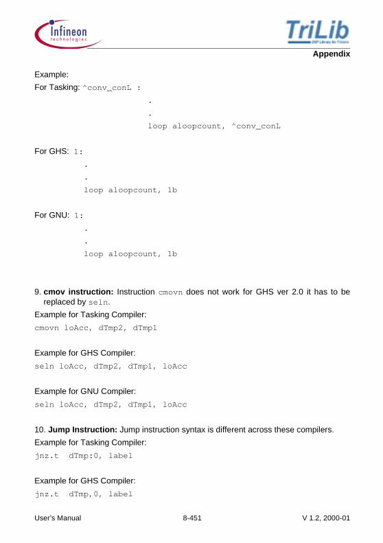
Appendix
Example:
For Tasking: ^conv_conL :
.
.
loop aloopcount, ^conv_conL
For GHS: 1:
.
.
loop aloopcount, 1b
For GNU: 1:
.
.
loop aloopcount, 1b
9. cmov instruction: Instruction cmovn does not work for GHS ver 2.0 it has to bereplaced by seln.
Example for Tasking Compiler:
cmovn loAcc, dTmp2, dTmp1
Example for GHS Compiler:
seln loAcc, dTmp2, dTmp1, loAcc
Example for GNU Compiler:
seln loAcc, dTmp2, dTmp1, loAcc
10. Jump Instruction: Jump instruction syntax is different across these compilers.
Example for Tasking Compiler:
jnz.t dTmp:0, label
Example for GHS Compiler:
jnz.t dTmp,0, label
User’s Manual 8-451 V 1.2, 2000-01

Appendix
Example for GNU Compiler:
jnz.t dTmp,0, label
Note:
The instruction jz works only for the GreenHills V2.0.2. For old versions of GreenHills thisinstruction is not supported.
User’s Manual 8-452 V 1.2, 2000-01

Glossary
9 Glossary
A
Acquisition Time The time required for a sample-and-hold (S/H) circuit to capture an input analog value. Specifically, the time for the S/H output to approximately equal its input.
Adaptive Delta Modulation (ADM)
A variation of delta modulation in which the step size may vary from sample to sample.
ADC (or A/D, Analog-to-Digital Converter)
The electronic component which converts the instantaneous value of an analog input signal to a digital word (represented as a binary number) for Digital Signal Processing. The ADC is the first link in the digital chain of signal processing.
ADPCM (Adaptive Differential Pulse Code Modulation)
A very fast data compression algorithm based on the differences occurring between two samples.
Algorithm A structured set of instructions and operations tailored to accomplish a signal processing task. For example, a Fast Fourier Transform (FFT), or a Finite Impulse Response (FIR) filter are common DSP algorithms.
Aliasing The problem of unwanted frequencies created when sampling a signal of a frequency higher than half the sampling rate.
All-Pass Filter A filter that provides only phase shift or phase delay without appreciable changing the magnitude characteristic.
Amplitude 1. Greatness of size, magnitude.2. Physics. The maximum absolute value of a periodically
varying quantity.3. Mathematics.
a) The maximum absolute value of a periodic curvemeasured along its vertical axis.
b) The angle made with the positive horizontal axis by thevector representation of a complex number.
4. Electronics. The maximum absolute value reached by avoltage or current waveform.
User’s Manual 9-453 V 1.2, 2000-01

Glossary
Analog A real world physical quantity or data, characterized by being continuously variable (rather than making discrete jumps),and can be as precise as the available measuring technique.
ANSI (American National Standards Institute)
A private organization that develops and publishes standards for voluntary use in the U.S.A.
Anti-Aliasing Filter A low-pass filter used at the input of digital audio converters to attenuate frequencies above the half-sampling frequency to prevent aliasing.
Anti-Imaging Filter A low-pass filter used at the output of digital audio converters to attenuate frequencies above the half-sampling frequency to eliminate image spectra present at multiples of the sampling frequency.
ASCII (pronounced "ask-ee") (American Standard Code for Information Interchange)
An ANSI standard data transmission code consisting of seven information bits, used to code 128 letters, numbers, and special characters. Many systems now use an 8-bit binary code, called ASCII-8, in which 256 symbols are represented (for example, IBM’s "extended ASCII").
Asymmetrical (non-reciprocal) Response
Term used to describe the comparative shapes of the boost/cut curves for variable equalizers. The cut curves do not mirror the boost curves, but instead are quite narrow, intended to act as notch filters.
Asynchronous A transmission process where the signal is transmitted without any fixed timing relationship between one word and the next (and the timing relationship is recovered from the data stream).
B
Bandpass Filter A filter that has a finite passband, neither of the cutoff frequencies being zero or infinite. The bandpass frequencies are normally associated with frequencies that define the half power points, i.e., the -3 dB points.
Band-Limiting Filters
A low-pass and a high-pass filter in series, acting together to restrict (limit) the overall bandwidth of a system.
User’s Manual 9-454 V 1.2, 2000-01

Glossary
Bandwidth Abbreviation. BW
The numerical difference between the upper and lower -3 dB points of a band of audio frequencies. Used to figure the Q, or quality factor for a filter.
Bilinear Transform A mathematical method used in the transformation of a continuous time (analog) function into an equivalent discrete time (digital) function. Fundamentally important for the design of digital filters. A bilinear transform ensures that a stable analog filter results in a stable digital filter, and it exactly preserves the frequency-domain characteristics, albeit with frequency compression.
Bit Error Rate The number of bits processed before an erroneous bit is found (e.g. 10E13), or the frequency of erroneous bits (e.g. 10E-13).
Bit Rate The rate or frequency at which bits appear in a bit stream. The bit rate of raw data from a CD, for example, is 4.3218 MHz.
Bit Stream A binary signal without regard to grouping.
Bit-Mapped Display
A display in which each pixel’s color and intensity data are stored in a separate memory location.
Boost/Cut Equalizer
The most common graphic equalizer. Available with 10 to 31 bands on octave to 1/3-octave spacing. The flat (0 dB) position locates all sliders at the center of the front panel. Comprised of bandpass filters, all controls start at their center 0 dB position and boost (amplify or make larger) signals by raising the sliders, or cut (attenuate or make smaller) the signal by lowering the sliders on a band-by-band basis. Commonly provide a center-detent feature identifying the 0 dB position. Proponents of boosting in permanent sound systems argue that cut-only use requires adding make-up gain which runsthe same risk of reducing system headroom as boosting.
Buffer In data transmission, a temporary storage location for information being sent or received.
Burst Error A large number of data bits lost on the medium because of excessive damage to or obstruction on the medium.
User’s Manual 9-455 V 1.2, 2000-01
Glossary
Bus One or more electrical conductors used for transmitting signals or power from one or more sources to one or more destinations. Often used to distinguish between a single computer system (connected together by a bus) and multi-computer systems connected together by a network.
C
Cartesian Coordinate System
1. A two-dimensional coordinate system in which thecoordinates of a point in a plane are its distances from twoperpendicular lines that intersect at an origin, the distancefrom each line being measured along a straight line parallelto the other.
2. A three-dimensional coordinate system in which thecoordinates of a point in space are its distances from eachof three perpendicular lines that intersect at an origin. Afterthe Latin form of Descartes, the mathematician whoinvented it.
Codec (Code-Decode)
A device for converting voice signals from analog to digital for use in digital transmission schemes, normally telephone based, and then converting them back again. Most codecs employ proprietary coding algorithms for data compression, common examples being Dolby’s AC-2, ADPCM, and MPEG schemes.
Compander A contraction of compressor-expander. A term referring to dynamic range reduction and expansion performed by first a compressor acting as an encoder, and second by an expander acting as the decoder. Normally used for noise reduction or headroom reasons.
Complex Frequency Variable
An AC frequency in complex number form.
Complex Number Mathematics
Any number of the form a + bj, where a and b are real numbers and j is an imaginary number whose square equals -1 and a represents the real part (e.g., the resistive effect of a filter, at zero phase angle) and b represents the imaginary part (e.g., the reactive effect, at 90 phase angle).
User’s Manual 9-456 V 1.2, 2000-01

Glossary
Compression 1. An increase in density and pressure in a medium, such asair, caused by the passage of a sound wave.
2. The region in which this occurs.
Compression Wave
A wave propagated by means of the compression of a fluid, such as a sound wave in air.
Constant-Q Equalizer (also Constant-Bandwidth)
Term applied to graphic and rotary equalizers describing bandwidth behavior as a function of boost/cut levels. Since Q and bandwidth are inverse sides of the same coin, the terms are fully interchangeable. The bandwidth remains constant for all boost/cut levels. For constant-Q designs, the skirts vary directly proportional to boost/cut amounts. Small boost/cut levels produce narrow skirts and large boost/cut levels produce wide skirts.
Convolution A mathematical operation producing a function from a certain kind of summation or integral of two other functions. In the time domain, one function may be the input signal, and the other the impulse response. The convolution than yields the result of applying that input to a system with the given impulse response. In DSP, the convolution of a signal with FIR filter coefficients results in the filtering of that signal.
Correlation A mathematical operation that indicates the degree to which two signals are alike.
Crest Factor The term used to represent the ratio of the peak (crest) value to the RMS value of a waveform.
Critical Band Physiology of Hearing
A range of frequencies that is integrated (summed together) by the neural system, equivalent to a bandpass filter (auditory filter) with approximately 10-20% bandwidth (approximately one-third octave wide).[Although the latest research says critical bands are more like 1/6-octave above 500 Hz, and about 100 Hz wide below 500Hz]. The ear can be said to be a series of overlapping critical bands, each responding to a narrow range of frequencies. Introduced by Fletcher (1940) to deal with the masking of a pure-tone by wideband noise.
User’s Manual 9-457 V 1.2, 2000-01

Glossary
Cut-Only Equalizer Term used to describe graphic equalizers designed only for attenuation. (Also referred to as notch equalizers, or band-reject equalizers). The flat (0 dB) position locates all sliders at the top of the front panel. Comprised only of notch filters (normally spaced at 1/3-octave intervals), all controls start at 0 dB and reduce the signal on a band-by-band basis. Proponents of cut-only philosophy argue that boosting runs the risk of reducing system headroom.
Cutoff Frequency Filters
The frequency at which the signal falls off by 3 dB (the half power point) from its maximum value. Also referred to as the -3 dB points, or the corner frequencies.
D
DAC (or D/A, Digital-to-Analog Converter)
The electronic component which converts digital words into analog signals that can then be amplified and used to drive loudspeakers, etc. The DAC is the last link in the digital chain of signal processing.
Decibel Abbreviation. dB
A unit used to express relative difference in power, intensity, voltage or other, between two acoustic or electric signals, equal to ten times (for power ratios - twenty times for all other ratios) the common logarithm of the ratio of the two levels. Equal to one-tenth of a bel.
Delta Modulation A single-bit coding technique in which a constant step size digitizes the input waveform. Past knowledge of the information permits encoding only the differences between consecutive values.
User’s Manual 9-458 V 1.2, 2000-01

Glossary
Delta-Sigma Modulation (also Sigma-Delta)
An analog-to-digital conversion scheme rooted in a design originally proposed in 1946, but not made practical until 1974 by James C. Candy. The name delta-sigma modulation was coined by Inose and Yasuda at the University of Tokyo in 1962, but due to a misunderstanding the words were interchanged and taken to be sigma-delta. Both names are still used for describing this modulator. Characterized by oversampling and digital filtering to achieve high performance at low cost, a delta-sigma A/D thus consists of an analog modulator and a digital filter. The fundamental principle behind the modulator is that of a single-bit A/D converter embedded in an analog negative feedback loop with high open loop gain. The modulator loop oversamples and processes the analog input at a rate much higher than the bandwidth of interest. The modulator’s output provides 1-bit information at a very high rate and in a format that a digital filter can process to extract higher resolution (such as 20-bits) at a lower rate.
Digital Audio Data Compression, commonly shortened to "Audio Compression."
Any of several algorithms designed to reduce the number of bits (hence, bandwidth and storage requirements) required for accurate digital audio storage and transmission. Characterized by being "lossless" or "lossy". The audio compression is "lossy" if actual data is lost due to the compression scheme, and "lossless" if it is not. Well designed algorithms ensure "lost" information is inaudible.
Digital Audio The use of sampling and quantization techniques to store or transmit audio information in binary form. The use of numbers (typically binary) to represent audio signals.
Digital Filter Any filter accomplished in the digital domain.
Digital Signal Any signal which is quantized (i.e., limited to a distinct set of values) into digital words at discrete points in time. The accuracy of a digital value is dependent on the number of bits used to represent it.
Digitization Any conversion of analog information into a digital form.
Discrete Fourier Transform (DFT)
A DSP algorithm used to determine the fourier coefficient corresponding to a set of frequencies, normally linearly spaced.
User’s Manual 9-459 V 1.2, 2000-01

Glossary
DSP (Digital Signal Processing)
A technology for signal processing that combines algorithms and fast number-crunching digital hardware and is capable of high-performance and flexibility.
F
FFT (Fast Fourier Transform)
A DSP algorithm that is the computational equivalent to performing a specific number of discrete fourier transforms, but by taking advantage of computational symmetries and redundancies, significantly reduces the computational burden.
FIR (Finite Impulse-Response) Filter
A commonly used type of digital filter. Digitized samples of the audio signal serve as inputs and each filtered output is computed from a weighted sum of a finite number of previous inputs. An FIR filter can be designed to have completely linear phase (i.e., constant time delay, regardless of frequency). FIR filters designed for frequencies much lower than the sample rate and/or with sharp transitions are computationally intensive with large time delays. Popularly used for adaptive filters.
Floating Point An encoding technique consisting of two parts: 1. A mantissa representing a fractional value with magnitude
less than one2. An exponent providing the position of the decimal point.
Floating point arithmetic allows the representation of verylarge or very small numbers with fewer bits.
Fourier Analysis Mathematics
The approximation of a function through the application of a Fourier Series to periodic data.
Fourier Series Application of the Fourier theorem to a periodic function, resulting in sine and cosine terms which are harmonics of the periodic frequency. (After Baron Jean Baptiste Joseph Fourier.)
Fourier Theorem A mathematical theorem stating that any function may be resolved into sine and cosine terms with known amplitudes and phases.
User’s Manual 9-460 V 1.2, 2000-01

Glossary
Frequency 1. The property or condition of occurring at frequent intervals.2. Mathematics. Physics. The number of times a specified
phenomenon occurs within a specified interval asa) The number of repetitions of a complete sequence of
values of a periodic function per unit variation of anindependent variable.
b) The number of complete cycles of a periodic processoccurring per unit time.
c) The number of repetitions per unit time of a completewaveform, as of an electric current.
G
Graphic Equalizer A multi-band variable equalizer using slide controls as the amplitude adjustable elements. Named for the positions of the sliders “graphing” the resulting frequency response of the equalizer. Only found on active designs. Center frequency and bandwidth are fixed for each band.
H
Harmonic Series 1. Mathematics. A series whose terms are in harmonicprogression as 1 + 1/3 + 1/5 + 1/7 +...
2. Music. A series of tones consisting of a fundamental toneand the overtones produced by it and whose frequencies areconsecutive integral multiples of the frequency of thefundamental.
High-Pass Filter A filter having a passband extending from some finite cutoff frequency (not zero) up to infinite frequency. An infrasonic filter is a high-pass filter.
I
IIR (Infinite Impulse-Response) Filter
A commonly used type of digital filter. This recursive structure accepts as inputs digitized samples of the audio signal and then each output point is computed on the basis of a weighted sum of past output (feedback) terms, as well as past input values. An IIR filter is more efficient than its FIR counterpart, but poses more challenging design issues. Its strength is in not requiring as much DSP power as FIR, while its weakness is not having linear group delay and possible instabilities.
User’s Manual 9-461 V 1.2, 2000-01

Glossary
Interpolating Response
Term adopted by Rane Corporation to describe the summing response of adjacent bands of variable equalizers using buffered summing stages. If two adjacent bands, when summed together, produce a smooth response without a dip in the center, they are said to interpolate between the fixed center frequencies, or combine well.
Inverse Square Law Sound Pressure Level
Sound propagates in all directions to form a spherical field, thus sound energy is inversely proportional to the square of the distance, i.e., doubling the distance quarters the sound energy (the inverse square law), so SPL is attenuated 6dB for each doubling.
Interleaving The process of rearranging data in time. Upon de-interleaving, errors in consecutive bits or words are distributed to a wider area to guard against consecutive errors in the storage media.
L
Linear PCM A pulse code modulation system in which the signal is converted directly to a PCM word without companding, or other processing.
Low-Pass Filter A filter having a passband extending from DC (zero Hz) to some finite cutoff frequency (not infinite). A filter with a characteristic that allows all frequencies below a specified rolloff frequency to pass and attenuate all frequencies above. Anti-aliasing and anti-imaging filters are low-pass filters.
M
Minimum-Phase Filters
Electrical circuits from an electrical engineering viewpoint, the precise definition of a minimum-phase function is a detailed mathematical concept involving positive real transfer functions, i.e., transfer functions with all zeros restricted to the left half s-plane (complex frequency plane using the Laplace transform operator s). This guarantees unconditional stability in the circuit. For example, all equalizer designs based on 2nd-order bandpass or band-reject networks have minimum-phase characteristics.
User’s Manual 9-462 V 1.2, 2000-01

Glossary
MIPS (Million Instructions Processed Per Second)
A measure of computing power.
MLS (Maximum-Length Sequences)
A time-domain-based analyzer using a mathematically designed test signal optimized for sound analysis. The test signal (a maximum-length sequence) is electronically generated and characterized by having a flat energy-vs-frequency curve over a wide frequency range. Sounding similar to white noise, it is actually periodic, with a long repetition rate. Similar in principle to impulse response testing - think of the maximum-length sequence test signal as a series of randomly distributed positive- and negative-going impulses.
N
Narrow-Band Filter Term popularized by equalizer pioneer C.P. Boner to describe his patented (tapped toroidal inductor) passive notch filters. Boner’s filters were very high Q (around 200) and extremely narrow (5 Hz at the -3 dB points). Boner used 100-150 of these sections in series to reduce feedback modes. Today’s usage extends this terminology to include all filters narrower than 1/3-octave. This includes parametrics, notch filter sets, and certain cut-only variable equalizer designs.
Noise Shaping A technique used in oversampling low-bit converters and other quantizers to shift (shape) the frequency range of quantizing error (noise and distortion). The output of a quantizer is fed back through a filter and summed with its input signal. Dither is sometimes used in the process. Oversampling A/D converters shift much of it out of the audio range completely. In this case, the in-band noise is decreased, which allows low-bit converters (such as delta-sigma) to equal or out-perform high-bit converters (those greater than 16 bits). When oversampling is not involved, the noise still appears to decrease by 12dB ormore because it is redistributed into less audible frequency areas. The benefits of this kind of noise shaping are usually reversed by further digital processing.
User’s Manual 9-463 V 1.2, 2000-01

Glossary
Nyquist Frequency The highest frequency that may be accurately sampled. The Nyquist frequency is one-half the sampling frequency. For example, the theoretical Nyquist Frequency of a CD system is 22.05 kHz.
O
Octave 1. Audio. The interval between any two frequencies having aratio of 2 to 1.
2. Music a) The interval of eight diatonic degrees between two tones,
one of which has twice as many vibrations per second asthe other.
b) A tone that is eight full tones above or below another giventone.
c) An organ stop that produces tones an octave above thoseusually produced by the keys played.
One-Third Octave 1. Term referring to frequencies spaced every one-third of anoctave apart. One-third of an octave represents a frequency1.26-times above a reference, or 0.794-times below thesame reference. The math goes like this: 1/3-octave = 2E1/3 = 1.260 and the reciprocal, 1/1.260 = 0.794. Therefore, forexample, a frequency 1/3-octave above a 1kHz referenceequals 1.26kHz (which is rounded-off to the ANSI-ISOpreferred frequency of "1.25 kHz" for equalizers andanalyzers), while a frequency 1/3-octave below 1 kHz equals794 Hz (labeled "800 Hz"). Mathematically it is significant tonote that, to a very close degree, 2E1/3 equals 10E1/10(1.2599 vs. 1.2589). This bit of natural niceness allows thesame frequency divisions to be used to divide and mark anoctave into one-thirds and a decade into one-tenths.
2. Term used to express the bandwidth of equalizers and otherfilters that are 1/3-octave wide at their -3dB (half-power)points.
3. Approximates the smallest region (bandwidth) humansreliably detect change. Compare with third-octave.
Oversampling A technique where each sample from the converter is sampled more than once, i.e., oversampled. This multiplication of samples permits digital filtering of the signal, thus reducing the need for sharp analog filters to control aliasing.
User’s Manual 9-464 V 1.2, 2000-01

Glossary
P
Parametric Equalizer
A multi-band variable equalizer offering control of all the "parameters" of the internal bandpass filter sections. These parameters being amplitude, center frequency and bandwidth. This allows the user not only to control the amplitude of each band, but also to shift the center frequency and to widen or narrow the affected area. Available with rotary and slide controls. Subcategories of parametric equalizers exist which allow control of center frequency but not bandwidth. For rotary control units the most used term is quasi-parametric. For units with slide controls the popular term is paragraphic. The frequency control may be continuously variable or switch selectable in steps. Cut-only parametric equalizers (with adjustable bandwidth or not) are called notch equalizers or band-reject equalizers.
Passive Equalizer A variable equalizer requiring no power to operate. Consisting only of passive components (inductors, capacitors and resistors) passive equalizers have no AC line cord. Favored for their low noise performance (no active components to generate noise), high dynamic range (no active power supplies to limit voltage swing), extremely good reliability (passive components rarely break), and lack of RFI interference (no semiconductors to detect radio frequencies). Disliked for their cost (inductors are expensive), size (and bulky), weight (and heavy), hum susceptibility (and need careful shielding) and signal loss characteristic (passive equalizers always reduce the signal). Also inductors saturate easily with large low frequency signals, causing distortion. Rarely seen today, but historically they were used primarily for notching in permanent sound systems.
PCM (Pulse Code Modulation)
A conversion method in which digital words in a bit stream represent samples of analog information. The basis of most digital audio systems.
Peaking Response Term used to describe a bandpass shape when applied to program equalization.
User’s Manual 9-465 V 1.2, 2000-01

Glossary
Period Abbreviation T, t
1. The period of a periodic function is the smallest time intervalover which the function repeats itself. (For example, theperiod of a sine wave is the amount of time T, it takes for thewaveform to pass through 360 degrees. Also, it is thereciprocal of the frequency itself, i.e., T = 1/f.)
2. Mathematics. a) The least interval in the range of the independent variable
of a periodic function of a real variable in which allpossible values of the dependent variable are assumed.
b) A group of digits separated by commas in a writtennumber.
c) The number of digits that repeat in a repeating decimal.For example, 1/7 = 0.142857142857... has a six-digitperiod.
Phaser also called a "Phase Shifter,"
This is an electronic device creating an effect similar to flanging, but not as pronounced. Based on phase shift (frequency dependent), rather than true signal delay (frequency independent), the phaser is much easier and cheaper to construct. Using a relatively simple narrow notch filter (all-pass filters also were used) and sweeping it up anddown through some frequency range, then summing this output with the original input, creates the desired effect. Narrow notch filters are characterized by having sudden and rather extreme phase shifts just before and just after the deep notch. This generates the needed phase shifts for the ever-changing magnitude cancellations.
Phase Shift The fraction of a complete cycle elapsed as measured from a specified reference point and expressed as an angle out of phase. In an un-synchronized or un-correlated way.
Phase Delay A phase-shifted sine wave appears displaced in time from the input waveform. This displacement is called phase delay.
Phasor 1. A complex number expressing the magnitude and phase ofa time-varying quantity. It is math shorthand for complexnumbers. Unless otherwise specified, it is used only withinthe context of steady-state alternating linear systems.(Example: 1.5 /27° is a phasor representing a vector with amagnitude of 1.5 and a phase angle of 27 degrees.)
2. For some unknown reason, used a lot by Star Fleetpersonnel.
User’s Manual 9-466 V 1.2, 2000-01

Glossary
Pink Noise Pink noise is a random noise source characterized by a flat amplitude response per octave band of frequency (or any constant percentage bandwidth), i.e., it has equal energy, or constant power, per octave. Pink noise is created by passingwhite noise through a filter having a 3 dB/octave roll-off rate. See white noise discussion for details. Due to this roll-off, pinknoise sounds less bright and richer in low frequencies than white noise. Since pink noise has the same energy in each 1/3-octave band, it is the preferred sound source for many acoustical measurements due to the critical band concept of human hearing.
Polarity A signal’s electromechanical potential with respect to a reference potential. For example, if a loudspeaker cone movesforward when a positive voltage is applied between its red and black terminals, then it is said to have a positive polarity. Amicrophone has positive polarity if a positive pressure on its diaphragm results in a positive output voltage.
Pre-Emphasis A high-frequency boost used during recording, followed by de-emphasis during playback, designed to improve signal-to-noise performance.
Proportional-Q Equalizer (also Variable-Q)
Term applied to graphic and rotary equalizers describing bandwidth behavior as a function of boost/cut levels. The term "proportional-Q" is preferred as being more accurate and less ambiguous than "variable-Q." If nothing else, "variable-Q" suggests the unit allows the user to vary (set) the Q, when no such controls exist. The bandwidth varies inversely proportional to boost (or cut) amounts, being very wide for small boost/cut levels and becoming very narrow for large boost/cut levels. The skirts, however, remain constant for all boost/cut levels.
Psychoacoustics The scientific study of the perception of sound.
PWM (Pulse Width Modulation)
A conversion method in which the widths of pulses in a pulse train represent the analog information.
Q
Quantization Error Error resulting from quantizing an analog waveform to a discrete level. In general the longer the word length, the less the error.
User’s Manual 9-467 V 1.2, 2000-01

Glossary
Quantization The process of converting, or digitizing, the almost infinitely variable amplitude of an analog waveform to one of a finite series of discrete levels. Performed by the A/D converter.
R
Real-Time Operation
What is perceived to be instantaneous to a user (or more technically, processing which completes in a specific time allotment).
Reconstruction Filter
A low-pass filter used at the output of digital audio processors (following the DAC) to remove (or at least greatly attenuate) any aliasing products (image spectra present at multiples of the sampling frequency) produced by the use of real-world (non-brickwall) input filters.
Recursive A data structure that is defined in terms of itself. For example, in mathematics, an expression, such as a polynomial, each term of which is determined by application of a formula to preceding terms. Pertaining to a process that is defined or generated in terms of itself, i.e., its immediate past history.
Rotary Equalizer A multi-band variable equalizer using rotary controls as the amplitude adjustable elements. Both active and passive designs exist with rotary controls. Center frequency and bandwidth are fixed for each band.
S
Sample Rate Conversion
The process of converting one sample rate to another, e.g. 44.1kHz to 48kHz. Necessary for the communication and synchronization of dissimilar digital audio devices, e.g., digital tape machines to CD mastering machines.
Sample-and-Hold (S/H)
A circuit which captures and holds an analog signal for a finite period of time. The input S/H proceeds the A/D converter, allowing time for conversion. The output S/H follows the D/A converter, smoothing glitches.
Sampling (Nyquist)Theorem
A theorem stating that a bandlimited continuous waveform may be represented by a series of discrete samples if the sampling frequency is at least twice the highest frequency contained in the waveform.
User’s Manual 9-468 V 1.2, 2000-01

Glossary
Sampling Frequency or Sampling Rate
The frequency or rate at which an analog signal is sampled or converted into digital data. Expressed in Hertz (cycles per second). For example, compact disc sampling rate is 44,100 samples per second or 44.1kHz, however in pro audio other rates exist, common examples being 32kHz, 48kHz and 50kHz.
Sampling The process of representing the amplitude of a signal at a particular point in time.
S/N ratio (Signal-to-Noise ratio)
The ratio of signal level (or power) to noise level (or power), normally expressed in decibels.
T
Third-Octave Term referring to frequencies spaced every three octaves apart. For example, the third-octave above 1kHz is 8kHz. Commonly misused to mean one-third octave. While it can be argued that "third" can also mean one of three equal parts and as such might be used to correctly describe one part of an octave spit into three equal parts, it is potentially too confusing.The preferred term is one-third octave.
Transversal Equalizer
A multi-band variable equalizer using a tapped audio delay line as the frequency selective element, as opposed to bandpass filters built from inductors (real or synthetic) and capacitors. The term "transversal filter" does not mean "digital filter". It is the entire family of filter functions done by means of a tapped delay line. There exists a class of digital filters realized as transversal filters, using a shift register rather than an analog delay line, with the inputs being numbers rather than analog functions.
W
Wavelength Symbol (Greek lower-case Lambda)
The distance between one peak or crest of a sine wave and the next corresponding peak or crest. The wavelength of any frequency may be found by dividing the speed of sound by the frequency.
User’s Manual 9-469 V 1.2, 2000-01

Glossary
White Noise Analogous to white light containing equal amounts of all visible frequencies, white noise contains equal amounts of all audible frequencies (technically the bandwidth of noise is infinite, but for audio purposes it is limited to just the audio frequencies). From an energy standpoint white noise has constant power per hertz (also referred to as unit bandwidth), i.e., at every frequency there is the same amount of power (while pink noise, for instance, has constant power per octave band of frequency). A plot of white noise power vs. frequency is flat if the measuring device uses the same width filter for all measurements. This is known as a fixed bandwidth filter. For instance, a fixed bandwidth of 5 Hz is common, i.e., the test equipment measures the amplitude at each frequency using a filter that is 5 Hz wide. It is 5 Hz wide when measuring 50 Hz or 2 kHz or 9.4 kHz, etc. A plot of white noise power vs. frequency change is not flat if the measuring device uses a variable widthfilter. This is known as a fixed percentage bandwidth filter. A common example of which is 1/3-octave wide, which equals a bandwidth of 23%. This means that for every frequency measured the bandwidth of the measuring filter changes to 23% of that new center frequency. For example the measuring bandwidth at 100 Hz is 23 Hz wide, then changes to 230 Hz wide when measuring 1 kHz, and so on. Therefore the plot of noise power vs. frequency is not flat, but shows a 3 dB rise in amplitude per octave of frequency change. Due to this rising frequency characteristic, white noise sounds very bright and lacking in low frequencies.
Z
Z-Transform A mathematical method used to relate coefficients of a digital filter to its frequency response, and to evaluate stability of the filter. It is equivalent to the Laplace transform of sampled data and is the building block of digital filters.
User’s Manual 9-470 V 1.2, 2000-01

"Microcontrollers" Templatefor Technical Documentation
AAdaptive Digital Filters 197
CplxDlms_4_16 214CplxDlmsBlk_4_16 222Dlms_2_16x32 229Dlms_4_16 201DlmsBlk_2_16x32 235DlmsBlk_4_16 208
Applications 401Equalizer 406Hardware Setup for Applications 408Oscillators 404Spectrum Analyzer 401
Argand Diagram 32Argument Conventions 29
aR 30CplxL 30CplxS 30cptrDataS 30DataD 29DataL 29DataS 29nH 29
BBuilding DSPLIB 18
CCanonical Form (Direct Form II) Second-order Section 174Cascaded Biquad IIR Filter 175Complex Arithmetic 32
Addition 32Conjugate 33Magnitude 33Multiplication 32Phase 33Shift 33Subtraction 32
Complex Arithmetic Functions 31CplxAdd_16 36CplxAdd_32 61CplxAdds_16 38
User’s Manual 471 V 1.1, 2000-01

"Microcontrollers" Templatefor Technical Documentation
CplxAdds_32 63CplxConj_16 49CplxConj_32 74CplxMag_16 51CplxMag_32 76CplxMul_16 44CplxMul_32 69CplxMuls_16 46CplxMuls_32 71CplxPhase_16 54CplxPhase_32 79CplxShift_16 59CplxShift_32 83CplxSub_16 40CplxSub_32 65CplxSubs_16 42CplxSubs_32 67
Complex Data Structure 35ANSI C 35GHS 35Tasking 35
Complex FunctionsCplxSub_16 40CplxSubs_16 42
Complex Number Representation 31Exponential form 31Magnitude and angle form 31Rectangular form 31Trigonometric form 31
Complex Number Schematic 34Complex Plane 31
DDesign of Test Cases for the FFT functions 256Directory Structure 17, 430, 445, 446, 447Discrete Cosine Transform
DCT_2_8 319IDCT_2_8 324
Discrete Cosine Transform (DCT) 309DSP Library Notations 23
FFast Fourier Transforms 241
User’s Manual 472 V 1.1, 2000-01

"Microcontrollers" Templatefor Technical Documentation
FFT_2_16 261FFT_2_16X32 293FFT_2_32 277FFTReal_2_16 269FFTReal_2_16x32 301FFTReal_2_32 285IFFT_2_16 265IFFT_2_16X32 297IFFT_2_32 281IFFTReal_2_16 273IFFTReal_2_16X32 305IFFTReal_2_32 289
Features 15FIR Filters 106
Multirate FiltersFirDec_16 156FirInter_16 165
Normal FIR 106Fir_16 108Fir_4_16 121FirBlk_16 115FirBlk_4_16 126
Symmetric FIRFirSym_16 132FirSym_4_16 142FirSymBlk_16 137FirSymBlk_4_16 148
Function Descriptions 29Functional Implementation 250Future of TriLib 16
IIIR Filters 173
IirBiq_4_16 176IirBiq_5_16 187IirBiqBlk_4_16 182IirBiqBlk_5_16 192
Implementation of FFT to Process the Real Sequences of Data 254Installation and Build 17Installing DSPLIB 18Introduction 15Inverse Discrete Cosine Transform (IDCT) 314
User’s Manual 473 V 1.1, 2000-01

"Microcontrollers" Templatefor Technical Documentation
MMathematical Functions 329
AntiLn_16 348Arctan_32 336Cos_32 333Expn_16 351Ln_32 344Rand_16 361RandInit_16 360Sine_32 330Sqrt_32 340XpowY_32 353
Matrix Operations 363MatAdd_16 364MatMult_16 371MatSub_16 367MatTrans_16 376
Memory Issues 24Multidimensional DCT 315
OOptimization Approach 24Options in Library Configurations 26
RRegister Naming Conventions 30
a 30ca 30
SSource Files List 19Statistical Functions 379
ACorr_16 381Avg_16 397Conv_16 389
Support Information 16
TTriCore Implementation Note 248TriLib Content 17TriLib Data Types 23TriLib Implementation - A Technical Note 24
User’s Manual 474 V 1.1, 2000-01

"Microcontrollers" Templatefor Technical Documentation
VVector Arithmetic Functions 85
VecAdd 86VecDotPro 92VecMaxIdx 94VecMaxVal 100VecMinIdx 97VecMinVal 103VecSub 89
User’s Manual 475 V 1.1, 2000-01

"Microcontrollers" Templatefor Technical Documentation
User’s Manual 476 V 1.1, 2000-01

((477))

h t t p : / / w w w . i n f i n e o n . c o m
Published by Infineon Technologies AG
Infineon goes for Business Excellence
“Business excellence means intelligent approaches and clearly defined processes, which are both constantly under review and ultimately lead to good operating results.Better operating results and business excellence mean less idleness and wastefulness for all of us, more professional success, more accurate information, a better overview and, thereby, less frustration and more satisfaction.”
Dr. Ulrich Schumacher


