Unit 8: Normal Calculations | Faculty Guide | Page 1 Unit 8: Normal Calculations Prerequisites This unit requires familiarity with basic facts about normal distributions, which are covered in Unit 7, Normal Curves. In addition, students need some background on distributions, means, and standard deviations, which are covered in Units 3, 4, and 6, respectively. Additional Topic Coverage Additional coverage of normal curves can be found in The Basic Practice of Statistics, Chapter 3, The Normal Distributions. Activity Description The purpose of this activity is to help students understand the connection between finding the proportion of data that fall in specific intervals and the areas under a density curve over those intervals. Students are given a graph of a standard normal density curve on which a rectangular grid has been superimposed. This allows them to determine areas by counting the number of rectangles under the density curve over specific intervals. Students estimate proportions by estimating areas. After estimating a collection of proportions, they use a z-table to see how close their estimates were to the actual proportions. Materials Students will need either a hard copy of this activity or six copies of the standard normal curve from Figure 8.11. That curve has been reproduced on the next page so that it can be easily copied. In addition, they will need a copy of a z-table (or access to technology where they can find standard normal probabilities).
Transcript
Unit 8: Normal Calculations | Faculty Guide | Page 1
Unit 8: Normal Calculations
PrerequisitesThis unit requires familiarity with basic facts about normal distributions, which are covered in Unit 7, Normal Curves. In addition, students need some background on distributions, means, and standard deviations, which are covered in Units 3, 4, and 6, respectively.
Additional Topic CoverageAdditional coverage of normal curves can be found in The Basic Practice of Statistics, Chapter 3, The Normal Distributions.
Activity DescriptionThe purpose of this activity is to help students understand the connection between finding the proportion of data that fall in specific intervals and the areas under a density curve over those intervals. Students are given a graph of a standard normal density curve on which a rectangular grid has been superimposed. This allows them to determine areas by counting the number of rectangles under the density curve over specific intervals. Students estimate proportions by estimating areas. After estimating a collection of proportions, they use a z-table to see how close their estimates were to the actual proportions.
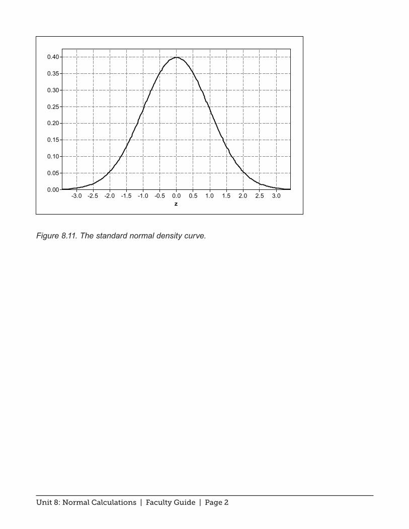
MaterialsStudents will need either a hard copy of this activity or six copies of the standard normal curve from Figure 8.11. That curve has been reproduced on the next page so that it can be easily copied. In addition, they will need a copy of a z-table (or access to technology where they can find standard normal probabilities).
Unit 8: Normal Calculations | Faculty Guide | Page 2
Figure 8.11. The standard normal density curve.
3.02.52.01.51.00.50.0-0.5-1.0-1.5-2.0-2.5-3.0
0.40
0.35
0.30
0.25
0.20
0.15
0.10
0.05
0.00
z
Unit 8: Normal Calculations | Faculty Guide | Page 3
The Video Solutions
1. The 68-95-99.7% Rule.
2. At least 5 feet 10 inches tall.
3. Suppose x is an observation from a normal distribution with mean μ and standard deviation σ. To calculate the z-score, subtract μ from x and then divide the result by σ .
4. The eligibility z-score for women (1.48) is higher than for men (0.98). So, in order to join the Beanstalks, women’s heights must be at least 1.48 standard deviations above the mean height for women while men’s heights need only be at least 0.98 standard deviations above the mean height for men.
Unit 8: Normal Calculations | Faculty Guide | Page 4
Unit Activity: Using Area to Estimate Standard Normal Proportions Solutions
1. Sample answer: 40
2. a. Sample answer: There are 20 rectangles in the shaded region below.
b. Proportion = 20/40 = 0.5
3. a. Sample answer: There are 6 ½ rectangles in the shaded region below.
b. Proportion = 6.5/40 ≈ 0.1625
3.02.52.01.51.00.50.0-0.5-1.0-1.5-2.0-2.5-3.0
0.40
0.35
0.30
0.25
0.20
0.15
0.10
0.05
0.00
z
3.02.52.01.51.00.50.0-0.5-1.0-1.5-2.0-2.5-3.0
0.40
0.35
0.30
0.25
0.20
0.15
0.10
0.05
0.00
z
Unit 8: Normal Calculations | Faculty Guide | Page 5
4. a. Sample answer: There is 1 rectangle in the shaded region below.
b. Proportion = 1/40 = 0.025
5. a. Sample answer: There are 33 ½ rectangles in the shaded region below.
b. Proportion = 33.5/40 = 0.8375
3.02.52.01.51.00.50.0-0.5-1.0-1.5-2.0-2.5-3.0
0.40
0.35
0.30
0.25
0.20
0.15
0.10
0.05
0.00
z
3.02.52.01.51.00.50.0-0.5-1.0-1.5-2.0-2.5-3.0
0.40
0.35
0.30
0.25
0.20
0.15
0.10
0.05
0.00
z
Unit 8: Normal Calculations | Faculty Guide | Page 6
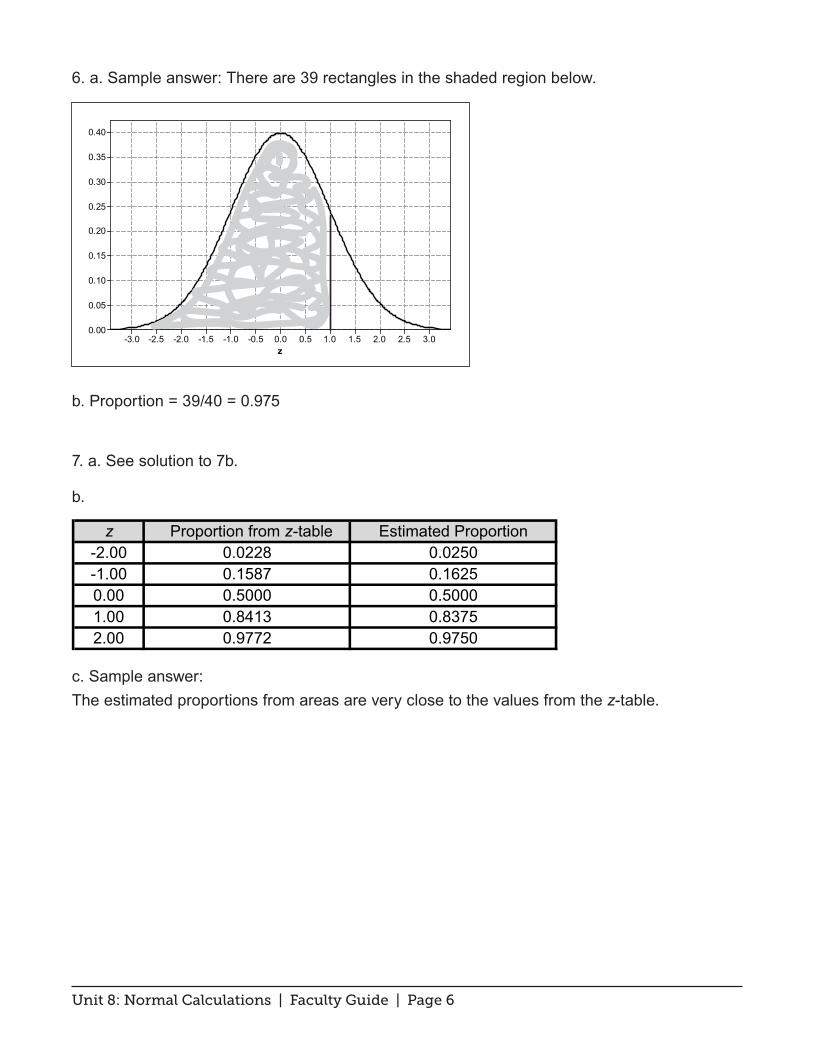
6. a. Sample answer: There are 39 rectangles in the shaded region below.
b. Proportion = 39/40 = 0.975
7. a. See solution to 7b.
b.
c. Sample answer: The estimated proportions from areas are very close to the values from the z-table.
3.02.52.01.51.00.50.0-0.5-1.0-1.5-2.0-2.5-3.0
0.40
0.35
0.30
0.25
0.20
0.15
0.10
0.05
0.00
z
z Proportion from z-table Estimated Proportion-2.00 0.0228 0.0250-1.00 0.1587 0.16250.00 0.5000 0.50001.00 0.8413 0.83752.00 0.9772 0.9750
Table 8.1(Unit Activity, 7b)
Unit 8: Normal Calculations | Faculty Guide | Page 7
Exercise Solutions
1. a. 65.5 – 2(2.5) = 60.5; 65.5 + 2(2.5) = 70.5
b. Around 95% of young women are between 60.5 and 70.5 inches tall (within two standard deviations of the mean). That means that 5% of young women are more than two standard deviations shorter or taller than the mean. Hence, 5%/2, or 2.5% of young women are more than 2 standard deviations taller than the mean.
c. 6 feet = 72 inches. Converting to a z-score gives z = (72 – 65.5)/2.5 = 2.6. This means that the 20-year-old woman is 2.6 standard deviations taller than the mean height of other young women.
2. a. We know that 68% of the scores are within 1 standard deviation of the mean – hence, between 400 and 600. That means that 32% are more than 1 standard deviation on either side of the mean. So, the percentage of scores above 600 is half of 32% or 16%.
b. Julie: z = (630 – 500)/100 = 1.3; John: z = (22 – 18)/6 ≈ 0.67. Julie did better than John because her score was 1.3 standard deviations above the mean while John’s score was only 0.67 standard deviations above the mean.
3. Sample answer: There are a few low priced homes, many moderately priced houses, some very expensive houses, and a few outrageously expensive mansions. So, the distribution of house prices is strongly skewed to the right and not normally distributed. The 68-95-99.7% rule should not be applied to house prices.
Heights of Young Women (in)60.5 70.565.5
Unit 8: Normal Calculations | Faculty Guide | Page 8
4. The table entry for z = -1 is 0.1587; so, 15.87% are less than -1.
The table entry for z = 2.25 is 0.9878; so, 98.78% are less than 2.25 and therefore, 1.22% are greater.
Because 98.78% are less than 2.25 and 15.87% are less than -1, the percentage lying between -1 and 2.25 is 98.78% - 15.87% = 82.91%, or about 83%.
Unit 8: Normal Calculations | Faculty Guide | Page 9
Review Questions Solutions
1. a.
b. This interval represents the data values that fall within one standard deviation of the mean. Using the 68-95-99.7 Rule, the percentage would be 68%. Thus, the proportion is 0.68.
c. To find the proportion of speeds that are below 30 mph or above 58 mph, subtract 0.68 from 1: 1 – 0.68 = 0.32. The proportion of speeds that are below 30 mph is half this amount: 0.32/2 = 0.16.
d. The speed of 72 mph is two standard deviations from the mean of 44. We know that roughly 0.95 of the speeds fall within two standard deviations from the mean. Hence, 0.05 of the speeds fall beyond two standard deviations from the mean. Roughly 0.05/2 or 0.025 of the speeds exceeded 72 mph.
2. Carrie’s standardized score on test B is z = (79 – 65)/9 = 1.56; Pat’s standardized score on test A is z = (85 – 78)/6 = 1.17. Carrie has the higher standardized score. If both tests cover the same material and both were taken by similar groups of students, then Carrie did better than Pat because her score is higher relative to the overall distribution of scores.
3. a. Convert 21 inches into a standardized value: z = (21 – 22.8)/1.1 ≈ - 1.64. Using the standard normal table we get a proportion of 0.0505 soldiers with head sizes below the one observed. That means that 1 – 0.0505, or a proportion of 0.9495, or 94.95% of soldiers has head sizes above 21 inches.
8672584430162Speed (mph)
Unit 8: Normal Calculations | Faculty Guide | Page 10
Using Minitab, we did not have to first convert to a z-score. The result is slightly more accurate because we did not round a z-score to two decimals.
b. Converting 23 inches into a standardized value gives: z = (23 – 22.8)/1.1 ≈ 0.18. Using the standard normal table, we get a proportion of 0.5714. The proportion of soldiers with head size between 21 inches and 23 inches is 0.5714 – 0.0505 = 0.5209, or around 52.09%.
Using Minitab, we did not have to first convert to z-scores or subtract two proportions. Note there is a slight difference in the proportion below compared to the one above due to rounding z-scores to two decimals.
Head Size (in)21
0.9491
22.8
Head Size (in)21
0.5213
23
Unit 8: Normal Calculations | Faculty Guide | Page 11
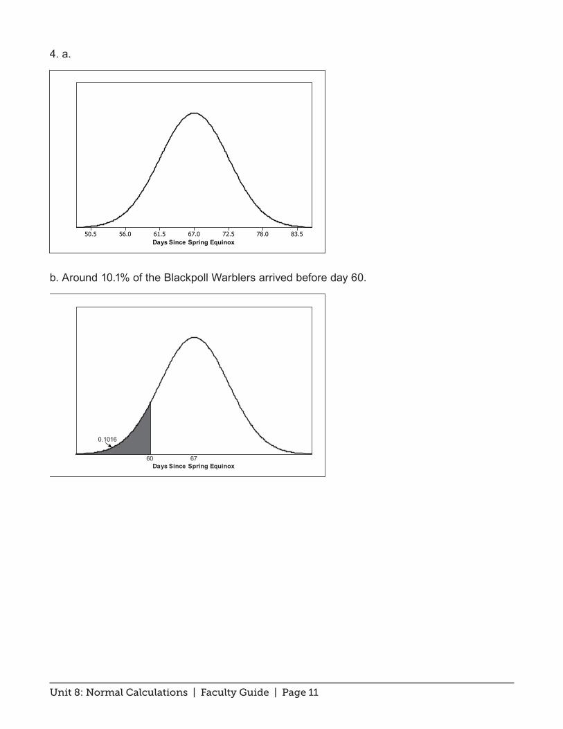
4. a.
b. Around 10.1% of the Blackpoll Warblers arrived before day 60.
83.578.072.567.061.556.050.5Days Since Spring Equinox
Days Since Spring Equinox60
0.1016
67
Unit 8: Normal Calculations | Faculty Guide | Page 12
c. Around 29.3% of the Blackpoll Warblers arrived after day 70.
d. Around 60.6% of the Blackpoll Warblers arrived between days 60 and 70.