University of Groningen

Interface and surface roughness of polymer-metal laminatesvan Tijum, Redmer

IMPORTANT NOTE: You are advised to consult the publisher's version (publisher's PDF) if you wish to cite fromit. Please check the document version below.

Document VersionPublisher's PDF, also known as Version of record

Publication date:2006

Link to publication in University of Groningen/UMCG research database

Citation for published version (APA):van Tijum, R. (2006). Interface and surface roughness of polymer-metal laminates. s.n.

CopyrightOther than for strictly personal use, it is not permitted to download or to forward/distribute the text or part of it without the consent of theauthor(s) and/or copyright holder(s), unless the work is under an open content license (like Creative Commons).

The publication may also be distributed here under the terms of Article 25fa of the Dutch Copyright Act, indicated by the “Taverne” license.More information can be found on the University of Groningen website: https://www.rug.nl/library/open-access/self-archiving-pure/taverne-amendment.

Take-down policyIf you believe that this document breaches copyright please contact us providing details, and we will remove access to the work immediatelyand investigate your claim.

Downloaded from the University of Groningen/UMCG research database (Pure): http://www.rug.nl/research/portal. For technical reasons thenumber of authors shown on this cover page is limited to 10 maximum.

Download date: 29-11-2021

109

6 Chapter 6

Roughness and adhesion

6.1 Introduction

In the previous chapters the adherence of a polymer coating to a metal substrate and

surface roughness are discussed as separate issues. This chapter will concentrate on the

combination of both but it should be realized that surface roughness appears at various

length scales. When two nominally flat bodies are brought into contact, the area of real

contact will usually be only a small fraction of the nominal contact area. The contact

surfaces can be regarded as an area with small asperities and depending on the

conditions, these asperities may deform either elastically or plastically.

The real contact area determines the system performance, e.g. how well the coating

adheres, the thermal conductivity and the friction. In 1882, Hertz [1] presented a

description of a frictionless normal contact of two elastic bodies of a quadratic profile.

He found that the area of real contact varies nonlinearly with the load according to 2

3~N

F . Almost a century later Archard [2] applied this solution to the contact between a

rough surface and an elastic body. He showed that a fractal-like surface can be

simplified by a distribution of asperities. In this case the contact area varies linearly with

NF . Also Bush et al. [3] found a linear relationship with the applied force

NF . Persson et

al. [4] compared the linear relationship with a numerical approach and arrived to the

same conclusion.

Already in the early eighties of the last century, it was recognized that rough

surfaces can be described by self-affine fluctuations [5]. The self-affine character was

used to study metal-polymer interfaces in combination with self-adhesion [6,7]. By

bringing a soft elastic body in contact with a rigid rough body, an energy balance will

originate between the adhesive energy, the surface energy and the elastic energy of the

soft elastic body.

In this chapter different aspects of adhesion will be presented. Firstly, a finite

element model study is employed on a fully wetted rigid rough substrate. The strength of

the interface is examined with a pull-off test under normal loading, where the maximum

stress is determined. In this particular case the roughness is responsible for an increase in

contact area. This study will show the effect of extreme surface roughness on the pull-

off force. The results of this are summarized in [8].

Secondly, the deformation of laminated steel is simulated. During this process many

phenomena occur simultaneously like e.g. substrate roughening, surface area changes,

Chapter 6

110

plastic deformation, elastic energy storage and a decrease or increase in adhesive energy.

The finite element modeling approach will give a description of the influence of each of

these effects. The results of this study are summarized in [9]. Finally, a linkage is made

between the numerical approach and an analytical description based on linear elastic

theory. In the latter a flat polymer plate is brought into contact with a self-affine rough

rigid surface.

In the following the effect of the self-affine roughness on the interface strength is

addressed. To determine the influence of the surface roughness on the interface strength

a finite element model is presented in which a cohesive zone defines the interface

between the polymer and the metal.

6.2 Theory

As shown in chapters 2 and 5, a metal surface roughens when deformed. A height-height

correlation function ( ),C r ε of the interface may be defined as [10]

( , ) ( , ) (0, )C r h r hε ε ε=�

, (6.1)

where ( ),h r ε�

is the height of the surface at a strain ε and at the position r�

. It has been

shown in chapters 2 and 5 and also in [11,12] that for all strains, ( ),C r ε of a surface of

a uniaxially deformed metal can be approximated by:

( )2 ( )2

( , ) ( ) exp[ / ( ) ]H

C r w rε

ε ε ξ ε≈ − . (6.2)

Eq. (6.2) describes the surface roughness in a statistical sense with three parameters: the

root-mean-square roughness amplitude w above a certain lateral correlation length ξ ,

and a Hurst exponent H characterizing the self-affine geometry below ξ . For a

uniaxially deforming metal these surface parameters are a function of the applied strain

ε . From experiments parameterized fits for ( )w ε , ( )H ε and ( )ξ ε may be determined

(see also chapter 5 and [11,8]).

Often, eq. (6.2) is expressed in terms of height differences, which is in fact a

variance:

( ) ( )( )2 ( )2 2( , ) 2 ( ) ( , ) 2 ( ) 1 exp[ / ( ) ]H

g r w C r w rε

ε ε ε ε ξ ε= − = − − , (6.3)

where ( , )g r ε is the height difference squared between 2 arbitrary surface points located

in a horizontal plane at a distance r from each other. In general, the maximum

resolution of a measurement technique defines the lower bound for r . Therefore the

minimum average height difference for the shortest distance minr can be defined as

min( , )g r ε and the relative surface area is described as:

Roughness and adhesion

111

2

min min

min

( , )real

nom

r g rA

A r

ε+= , (6.4)

where nom

A is the nominal area. For r ξ� eq. (6.3) can be approximated by

2 ( )

2 ( )( , ) | 2 ( )

( )

H

r

rg r w

ε

ξ

εε ε

ξ ε

=

�

. (6.5)

In general minr is much smaller than ξ and therefore eq. (6.4) can be rewritten as:

2

2( ( ) 1)

min2 ( )

2 ( )1

( )

Hreal

H

nom

A wr

A

ε

ε

ε

ξ ε−= + . (6.6)

When we take minr equal to unity, the relative surface area becomes

2 2 ( )1 2 ( ) ( ) Hreal

nom

Aw

A

εε ξ ε −= + . (6.7)

Fig. 6.1 shows the influence of H on the relative surface area. For a small H , an

extremely rough surface will appear, which has nearly twice the surface area of a flat

surface. For larger values of H , the increase in relative surface area is not so dramatic.

0.0 0.5 1.0 1.5 2.0 2.5 3.01.0

1.2

1.4

1.6

1.8

Re

lative

su

rfa

ce

are

a [-]

w [a.u.]

Fig. 6.1. Relative surface area as a function of the root-mean-square roughness w with ξ =

30 and different Hurst exponents: ( ⋅ ⋅ ) H = 0.3, ( -- ) H = 0.6 and ( − ) H = 0.9.

Chapter 6

112

6.3 Pull-off test

6.3.1 Constitutive model

Fig. 6.2 shows a schematic of the axisymmetrical pull-off test used. The axisymmetry is

indicated in the figure by the symmetry axis and is parallel to the loading direction. The

thickness of the polymer layer is 40 µm. Two cylindrical metal plates of 20 µm thick

and radius 2049 µm enclose the polymer. Due to the symmetry only half of this system

has to be modeled. A cohesive zone is placed between the metal and the polymer. The

polymeric and metal descriptions are based on quadrilaterals. In the model the size of

these cells is set to 1 µm x 1 µm for a flat interface.

The algorithm described in chapter 2 is used to generate self-affine rough interfaces.

These interfaces are implemented as a cohesive zone [13] in a finite element model [14]

(see chapter 2 and 5). This specific cohesive zone definition is chosen, because large

fluctuations on the surface will cause shear deformation and fracture instead of only

normal fracture. The coupling between shear and normal tractions makes it therefore

suitable for our system.

As a material system chromium-plated steel with a glycol modified polyethylene

terephthalate (PETG) coating was chosen. The stress-strain response of the PETG [15,

[16] was used. The modeled stress-strain behavior of the polymer is shown in Fig. 6.3.

Further a hypothetical polymer is displayed with similar properties. The primary

difference is that it has one half the Young’s modulus of PETG.

Fig. 6.2. Schematic cross-sectional representation of the finite element model. The model consists of two identical rough metal disks, which are glued together with polymer.

Fig. 6.3. Stress-strain response of (-) PETG and the (--) hypothetical polymer.

6.3.2 Determination of the cohesive zone parameters

For the determination of the shear and normal response of the cohesive zone peel-tests

were performed. For this test we used a tensile stage inside an environmental scanning

Roughness and adhesion

113

electron microscope (ESEM). In an ESEM it is possible to prevent charging of the

deformed polymer by introducing small amounts of water as charge carrier. From the

ESEM observations, i.e. from both plane and cross-sectional view (Fig. 6.4) we were

able to estimate the shape of the necking of the polymer coating. The opening angle at

the crack-tip was 20 degrees. The peel-tests were performed at 0 degrees, which means

fully under an applied shear force. Due to necking of the polymer the opening angle of

the crack-tip was around 20 degrees instead of 0 degrees. By performing several plane-

strain simulations with different shear to normal ratios we were able to reach agreement

with the experiment (Fig. 6.5).

Fig. 6.6. Response of the used cohesive zone: - normal traction; -- shear traction; .- normal traction at maximum shear stress; .. shear traction at maximum normal stress.

The determined cohesive zone had the characteristics shown in Fig. 6.6. The graph

explains the relationship between the normal and the shear traction. Due to loading the

Fig. 6.4. Environmental scanning electron microscopy image during a zero degrees peel-test.

Fig. 6.5. Simulation of a 30 µm thick coating during a 0 degrees peel-test.

Chapter 6

114

traction-separation law will result in a combination of opening and shearing (see also

chapter 4). When large shear traction is applied, the maximum normal traction is

reduced and vice versa. It is important to emphasize that normal and shear traction are

coupled.

6.3.3 Numerical experiment

During an experimental pull-off test the load increases until fracture occurs. At that

point the loading curve drops towards zero. In the model this instability occurs as well.

In Fig. 6.7 an example of the force-displacement curve is shown together with the

deformed mesh at maximum stress. During the displacement controlled test cohesive

zone elements start to fracture (the stress in the cohesive zone element has passed the

maximum value). Then, less cohesive zone elements have to carry the still increasing

global stress, which results in an increase in the number of fractured elements. In

experiments and in the numerical approach this fracture process is instable. In Fig. 6.6,

the cohesive zone is well defined for all displacements. Consequently, cohesive zone

elements can still carry load after reaching a certain maximum stress level. Therefore it

is quite well possible to determine the maximum stress level (in Fig. 6.7 expressed with

■).

Fig. 6.7. Stress displacement curve for w = 3; ξ = 29 and H = 0.6. The squares denote at

which stress the deformed mesh in the inset is taken.

6.3.4 Results of the pull-off test

We will present the mechanical performance for three different Hurst H exponents (0.3,

0.6 and 0.9) and rms roughness of 3 µm. For each H various surfaces with different

lateral correlation lengths ξ are created. Each of these surfaces were used in the finite

element model and resulted in a maximum stress. Fig. 6.8 shows that a system with

Roughness and adhesion

115

lower H reaches a larger maximum stress level before failure. Obviously this is caused

by the fact that the relative surface area is extremely high. Important is to emphasize that

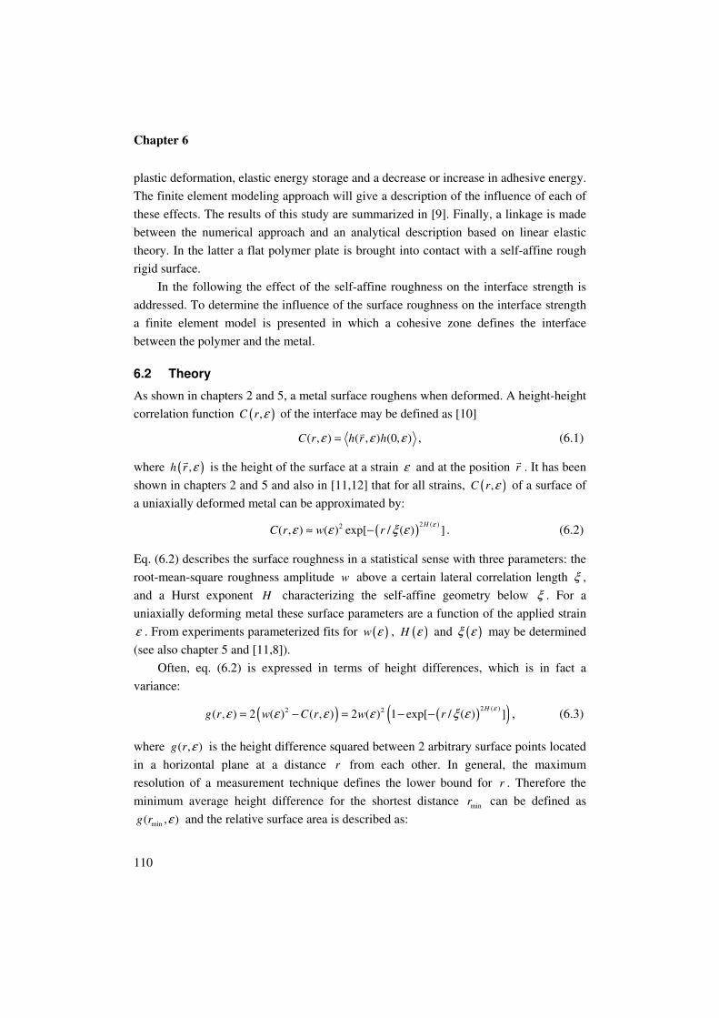
some ultimate stresses are larger than the yield stress of the polymer. Fig. 6.9 shows the

average phase angle ( )1tan ( ) / ( )t n

φ σ σ−= ∆ ∆ as a function of the relative surface area.

The increase in surface area involves a larger shear component at the interface. The ratio

of normal and shear components operating at the interface can be expressed as an angle

e.g.. This angle was calculated by the average of the absolute angle of shear and normal

stress over the whole surface at the maximum stress level. Fig. 6.9 shows that for large

roughness a cohesive zone also needs to incorporate shear stresses.

Fig. 6.8. Maximum stress as a function of the ratio /w ξ : ■ H = 0.3; ♦ H = 0.6; ▲ H = 0.9.

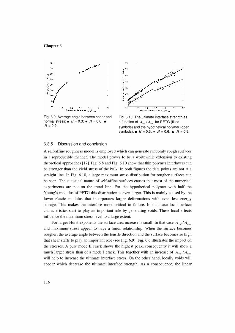
The maximum stress level can also be represented as a function of /real nom

A A . As

shown in Fig. 6.9 an increase of /real nom

A A causes an increase of the maximum stress

level. In the case of a small increase of the surface area the maximum stress level

increases linearly with the area increment. The relation holds up to relatively large

/real nom

A A but eventually a deviation from linearity occurs. Fig. 6.10 shows the results

for a hypothetical polymer that has one half the Young’s modulus of polyethylene

terephthalate (PETG) keeping the other properties fixed. Both curves show the same

response for increasing /real nom

A A . In both cases the cohesive zone is exactly the same.

Nevertheless, the change in the elastic modulus results in a smaller ultimate strength.

This is expected, as the lower Young’s modulus reduces the elastic energy storage. The

lower Young’s modulus incorporates larger strains and therefore displacements. The thin

polymer layer is therefore able to deform more homogeneously and becomes more

sensitive to the surface roughness and therefore a lower failure stress is found.

Chapter 6

116

6.3.5 Discussion and conclusion

A self-affine roughness model is employed which can generate randomly rough surfaces

in a reproducible manner. The model proves to be a worthwhile extension to existing

theoretical approaches [17]. Fig. 6.8 and Fig. 6.10 show that thin polymer interlayers can

be stronger than the yield stress of the bulk. In both figures the data points are not at a

straight line. In Fig. 6.10, a large maximum stress distribution for rougher surfaces can

be seen. The statistical nature of self-affine surfaces causes that most of the numerical

experiments are not on the trend line. For the hypothetical polymer with half the

Young’s modulus of PETG this distribution is even larger. This is mainly caused by the

lower elastic modulus that incorporates larger deformations with even less energy

storage. This makes the interface more critical to failure. In that case local surface

characteristics start to play an important role by generating voids. These local effects

influence the maximum stress level to a large extent.

For larger Hurst exponents the surface area increase is small. In that case /real nom

A A

and maximum stress appear to have a linear relationship. When the surface becomes

rougher, the average angle between the tensile direction and the surface becomes so high

that shear starts to play an important role (see Fig. 6.9). Fig. 6.6 illustrates the impact on

the stresses. A pure mode II crack shows the highest peak, consequently it will show a

much larger stress than of a mode I crack. This together with an increase of /real nom

A A

will help to increase the ultimate interface stress. On the other hand, locally voids will

appear which decrease the ultimate interface strength. As a consequence, the linear

Fig. 6.9. Average angle between shear and

normal stress: ■ H = 0.3; ♦ H = 0.6; ▲

H = 0.9.

Fig. 6.10. The ultimate interface strength as

a function of /real nom

A A for PETG (filled

symbols) and the hypothetical polymer (open

symbols): ■ H = 0.3; ♦ H = 0.6; ▲ H = 0.9.

Roughness and adhesion

117

relationship does not hold for small Hurst exponents or very small lateral correlation

lengths.

The impact of small interface effects is responsible for the larger deviations of the

maximum stress. These local effects amplify for polymers with lower Young’s moduli

strengthened by the reduced elastic energy storage.

6.4 Adhesion along metal-polymer interfaces during plastic deformation

In the manufacturing process severe plastic deformation is used to obtain the final

shapes of the end products. A drawback of plastic deformation is the intrinsic

roughening of the surface of the metal caused by plasticity. This section concentrates on

the implications of the roughening process for the mechanical properties of the

combined metal-polymer system. Clearly the subject is closely related to that of a large

number of papers discussing the impact of roughness on the work of adhesion W, e.g

[2,3,4,7,18,19,20]. However, our work detailed in [9] sets itself apart from earlier

research because it emphasizes on: First, the evolution of roughness of the metal as a

mechanical loading mechanism of a metal-polymer interface; second, the coupling

between the metal substrate and the polymer coating using a stress-separation law; and

third, the polymer behavior including yielding, softening and hardening. In the following

these points are briefly discussed in the framework of the current understanding.

The topics addressed here are the work of adhesion W between such a self-affine

roughening metal-polymer system, the dependence of W on the parameters w, H and ξ,

and the evolution of W as a function of uniaxial strain ε.

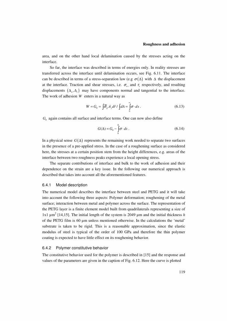
Fig. 6.11 illustrates the problem under consideration, and introduces a number of

relevant quantities. It shows a metal and polymer in contact across an interface at zero

Fig. 6.11. Schematic representation of some model parameters at two stages in the deformation process ( ε = 0 and ε > 0).

Chapter 6

118

strain, and also at a higher strain value. During straining the area of contact increases,

the average stress in the polymer increases, and roughness develops at the interface,

which is accompanied by stress concentrations. These stress concentrations may lead to

local delamination. Also, note the appearance of shear bands in the polymer, caused by

the intrinsic softening that characterizes the post-yield deformation behavior of typical

glassy polymers. The impact of all of these phenomena on the work of adhesion W is the

subject of this section.

For a metal (m) and a polymer (p) coming into contact across an area A0 the work of

adhesion W per unit area is defined as:

0 2m p mp

W G γ γ γ= = + − , (6.8)

where γm and γp represent the surface tension and γpm the interface energy. During

uniaxial deformation at a strain ε the nominal (projected) contact area nom

A is given by:

0( ) (1 )nom

A Aε ε= + . (6.9)

Due to roughening of the metal surface the real contact area real

A at a strain ε is larger

than Anom(ε) and is given by

( ) ( )real

A dA rε = ∫�

, (6.10)

where the integral is taken over all positions r�

on the nominal surface.

The work of adhesion ( )W ε at a strain ε can be approximated by:

( ) ( )( ) ( ) ( )

( ) ( )( ) ( )

h

E E E

nom nom nom

G r dA rU U UW G

A A A

εε ε εε ε

ε ε

+= − = −

∫� �

, (6.11)

where ( )G ε represents all surface and interface terms and ( )E

U ε is the elastic energy

stored in the bulk of the materials. The elastic energy is split in two terms:

First, ( )E

Uε ε represents the average energy stored in a deformed block of material

in case the surface does not roughen and may be approximated by

2

1

2

( )( )

E nom

pol

U dAE

ε σ εε = , (6.12)

where d is the layer thickness, pol

E is the Young’s modulus of the polymer. Due to the

substantial difference of the elastic moduli the metal can be regarded as a rigid solid and

is omitted from the energy balance.

Second, ( )h

EU ε represents the elastic energy contribution of the roughening

interface. The term ( ) ( ) ( ) /nom

G G r dA r Aε = ∫� �

takes into account the two competing

effects of roughening on the interface energy, on the one hand an increase in real contact

Roughness and adhesion

119

area, and on the other hand local delamination caused by the stresses acting on the

interface.

So far, the interface was described in terms of energies only. In reality stresses are

transferred across the interface until delamination occurs, see Fig. 6.11. The interface

can be described in terms of a stress-separation law (e.g ( )σ ∆ with ∆ the displacement

at the interface. Traction and shear stresses, i.e. n

σ , and tτ respectively, and resulting

displacements ( ),n t

∆ ∆ may have components normal and tangential to the interface.

The work of adhesion W enters in a natural way as

0

0

. /ij j

W G n dr dA dsσ σ∞

= = = ⋅∫ ∫ ∫� �

. (6.13)

0G again contains all surface and interface terms. One can now also define

0

0

( )G G dsσ∆

∆ = − ⋅∫ . (6.14)

In a physical sense ( )G ∆ represents the remaining work needed to separate two surfaces

in the presence of a pre-applied stress. In the case of a roughening surface as considered

here, the stresses at a certain position stem from the height differences, e.g. areas of the

interface between two roughness peaks experience a local opening stress.

The separate contributions of interface and bulk to the work of adhesion and their

dependence on the strain are a key issue. In the following our numerical approach is

described that takes into account all the aforementioned features.

6.4.1 Model description

The numerical model describes the interface between steel and PETG and it will take

into account the following three aspects: Polymer deformation; roughening of the metal

surface; interaction between metal and polymer across the surface. The representation of

the PETG layer is a finite element model built from quadrilaterals representing a size of

1x1 µm2 [14,15]. The initial length of the system is 2049 µm and the initial thickness h

of the PETG film is 60 µm unless mentioned otherwise. In the calculations the ‘metal’

substrate is taken to be rigid. This is a reasonable approximation, since the elastic

modulus of steel is typical of the order of 100 GPa and therefore the thin polymer

coating is expected to have little effect on its roughening behavior.

6.4.2 Polymer constitutive behavior

The constitutive behavior used for the polymer is described in [15] and the response and

values of the parameters are given in the caption of Fig. 6.12. Here the curve is plotted

Chapter 6

120

as a function of the true strain εtrue , which is defined as ( )ln 1true

ε ε= + . The regime of

the polymer is purely elastic and after yielding the polymer starts to soften. In this

regime shear bands occur as a result of localization. Eventually, the hardening phase will

stop the localization.

6.4.3 Roughening of the metal surface

One of the simplifications in the approach proposed here is to parameterize the

roughness evolution of a metal surface as a function of strain, and to assume that the

roughness evolution at a polymer-metal interface is essentially identical to this because

of the large difference in elastic moduli of typical metals (~100s of GPa) and glassy

polymers (~ 1GPa).

The surface morphology for as received rolled stainless steel (with an averaged

grain size equal to 11.7 µm and a plate thickness of 500 µm) was determined

experimentally with confocal microscopy [11] during uniaxial tensile experiments and

characterized by the following empirical relationships as a function of strain ε:

( ) 1

0

(1 )

( ) (1 ),

C

satw w e

εε

ξ ε ξ ε

−= −

= + (6.15)

with sat

w = 1.1 µm, C1 = 6.1 and ξ0 = 35 µm. The Hurst exponent H was found to be

insensitive to strain and is taken to be constant H(ε) = H0 = 0.6. The correlation length ξ

increases with the strain in the tensile direction. A qualitatively similar behavior was

0.0 0.1 0.2 0.3 0.40

10

20

30

40

50

σxx [M

Pa

]

εtrue

[-]

Fig. 6.12. Stress-strain relationship for PET, using the following values as defined in [15]:

0/E s = 7.76;

0/

sss s = 0.774;

0/As T = 91.99;

0/h s = 3.90; α = 0.25; N = 12.602;

0/

RC s =

0.132.

Roughness and adhesion

121

also found for other materials (Fe, Al, [12]). From experimental results least square fits

to eq. (6.15) were performed [11]. A recursive refinement algorithm (see chapter 2) was

used to simulate surfaces with the characteristics described by eq. (6.15). A detailed

example of the roughness evolution in the numerical model is displayed in chapter 2, a

few stages of which are apparent from Fig. 6.13.

6.4.4 Interaction between metal and polymer

In finite element models, stress-separation laws are commonly known as “cohesive

zones” and different kinds have been discussed in literature. In the numerical

calculations presented here the interface was implemented as a rate-independent mixed-

mode cohesive zone of the type described in [13]. This type defines coupled stress

separation laws ( , )n n t

σ ∆ ∆ (tractions) and ( , )t n t

τ ∆ ∆ (shear stresses) at the interface,

with n

∆ and t

∆ coordinates normal and parallel to the interface, respectively. The

distance ∆0 is defined as the point at which the opening stress n

σ attains its maximum

value max

nσ . Unless stated otherwise, the parameters used for the cohesive zone in this

section are: normal-to-shear stress ratio max max/n t

σ τ = 0.75, interface energy 0

CZG = 30

J/m2, working distance ∆0 = 300 nm and max

nσ = 36.8 MPa. To illustrate the key features

of the cohesive zone ( ,0)n n

σ ∆ is shown in Fig. 6.14.

For each interface element the surface area and stress state are calculated. The

interface energy can be calculated analogously to eq. (6.14) as:

Fig. 6.13. Typical results of stress fields in the PETG caused by strain induced roughening of

the substrate, showing xx

σ in the PET. Three cases are shown for true

ε in the elastic (top),

softening (middle) and hardening (bottom) region of the polymer stress-strain curve.

Chapter 6

122

0 , ,

0 0

( ) ( ) ( )n t

CZ CZ CZ CZ

i i n i tG G dn dtε σ ε τ ε

∆ ∆

= − −∫ ∫ , (6.16)

where 0

CZG refers to 0G of the cohesive zone (see eq. (6.13)), ,

CZ

i nσ is the stress normal

and ,

CZ

i tτ the stress parallel to the interface element i. In this work we are interested in

( )W ε and therefore in ( )G ε and ( )U ε . In the context of the numerical model we

define ( )G ε as follows:

1

( ) ( )

( )

N

CZ

i i

CZ i

nom

G A

GA

ε ε

ε ==∑

, (6.17)

with i running over the discrete elements in the model, ( )i

A ε and ( )CZ

iG ε are the

surface area and the interface energy of the i -th element, respectively.

Since all energies in the following are derived from the numerical model the

superscript CZ will be dropped.

6.4.5 Simulation of deformation

In the calculations the composite is loaded in uniaxial plane strain up to strains of 50%

(in steps of 0.1%). At each step the following boundary conditions (see Fig. 6.15) are

imposed on the PETG and the cohesive zone. At the side of the PETG at x = 0

displacements along x are imposed while displacements along y are free. Similar

boundary conditions are applied at x = L(ε). Along the interface displacements in the

substrate are constrained in all directions. Displacements in the polymer are not

restricted and they are coupled to those in the substrate by the stress-separation laws

0 2 4 6 8 100

10

20

30

40

G(∆)

σn [

MP

a]

∆n/∆

0 [-]

0 2 4 6 8 100

10

20

30

G [J/m

2]

∆n/∆

0 [-]

G(∆)

Fig. 6.14. Characteristics of the cohesive zone (a) ( , 0)n n

σ ∆ plotted as function of 0

/n

∆ ∆ (b)

( ) ( , 0)n

n nG n dnσ

∞

∆∆ = ∫ plotted as function of

0/

n∆ ∆ .

Roughness and adhesion

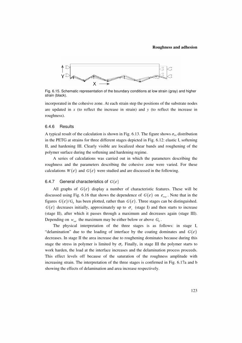
123

incorporated in the cohesive zone. At each strain step the positions of the substrate nodes

are updated in x (to reflect the increase in strain) and y (to reflect the increase in

roughness).

6.4.6 Results

A typical result of the calculation is shown in Fig. 6.13. The figure shows σxx distribution

in the PETG at strains for three different stages depicted in Fig. 6.12: elastic I, softening

II, and hardening III. Clearly visible are localized shear bands and roughening of the

polymer surface during the softening and hardening regime.

A series of calculations was carried out in which the parameters describing the

roughness and the parameters describing the cohesive zone were varied. For these

calculations ( )W ε and ( )G ε were studied and are discussed in the following.

6.4.7 General characteristics of ( )G ε

All graphs of ( )G ε display a number of characteristic features. These will be

discussed using Fig. 6.16 that shows the dependence of ( )G ε on true

ε . Note that in the

figures ( ) 0/G Gε has been plotted, rather than ( )G ε . Three stages can be distinguished.

( )G ε decreases initially, approximately up to y

σ (stage I) and then starts to increase

(stage II), after which it passes through a maximum and decreases again (stage III).

Depending on sat

w the maximum may be either below or above 0G .

The physical interpretation of the three stages is as follows: in stage I,

“delamination” due to the loading of interface by the coating dominates and ( )G ε

decreases. In stage II the area increase due to roughening dominates because during this

stage the stress in polymer is limited by σy. Finally, in stage III the polymer starts to

work harden, the load at the interface increases and the delamination process proceeds.

This effect levels off because of the saturation of the roughness amplitude with

increasing strain. The interpretation of the three stages is confirmed in Fig. 6.17a and b

showing the effects of delamination and area increase respectively.

Fig. 6.15. Schematic representation of the boundary conditions at low strain (gray) and higher strain (black).

Chapter 6

124

0.0 0.1 0.2 0.3 0.4

0.85

0.90

0.95

1.00

1.05

IIIII

G(ε

)/G

0 [-]

εtrue

[-]

I

Fig. 6.16. Normalized interface energy 0

( ) /G Gε as a function of ε for different values of sat

w

: � sat

w = 1.1 µm; � sat

w = 2.2 µm; � sat

w = 3.3 µm; � sat

w = 4.4 µm and � sat

w = 5.5 µm.

Here it is useful to split the effect of the roughness and the increase in surface area

(as shown in Fig. 6.17a and b):

0

( )( ) ( )

( )

real

nom

AG G G

A

εε ε

ε= + ∆ , (6.18)

where the effect of the roughness on the interface energy is

1

1

( ) ( )

( )

( )

N

i i

i

N

i

i

G A

G

A

ε ε

ε

ε

=

=

∆ = −∑

∑ (6.19)

and the surface area increase effect is

1

( )( )

( ) ( )

N

i

real i

nom nom

AA

A A

εε

ε ε==∑

. (6.20)

Fig. 6.17a shows the reduction in interface energy as indicated in eq. (6.19). This

effectively removes the effect of increasing area and gives an indication of the decrease

in ( )G ε caused by the loading of the interface. At the onset ( )G ε∆ decreases rapidly,

i.e. approximately linearly with w2. At the yield point of the polymer the rate of decrease

of ( )G ε∆ reduces considerably, and in fact for low sat

w the interface partly recovers due

to the softening of the polymer layer.

Roughness and adhesion

125

0.0 0.1 0.2 0.3 0.4-0.25

-0.20

-0.15

-0.10

-0.05

0.00

∆G

(ε)/

G0 [-]

εtrue

[-]

0,0 0,1 0,2 0,3 0,4

1,00

1,05

1,10

1,15

1,20

Are

al(ε

)/A

nom(ε

) [-

]

εtrue

[-]

Fig. 6.17. Normalized interface energy 0

( ) /G Gε (same data as in Fig. 6.16) separated into the

contribution (a) 0

( ) /G Gε∆ and (b) ( ) / ( )real nom

A Aε ε .

Fig. 6.17b shows ( ) /real nom

A Aε which exhibits a monotonous increase due to

roughening up to a maximum where the increase in nominal area starts dominating the

effects of the increase of w(ε).

6.4.8 ( )G ε as a function of w, H and ξ

In the previous section the general behavior of ( )G ε was illustrated, and curves at

different sat

w were presented. The situation remains about the same if we change other

parameters describing the self-affinity, the correlation length ξ and the Hurst exponent

H. A low value of H results in a rapid fluctuation on a shorter length scale, and this leads

to a larger decrease in ( )G ε at lower strains (Fig. 6.18a) and to a continuing

delamination above the yield point. However, the overall effect is still compensated by

the faster increase in surface area (Fig. 6.18b).

0.0 0.1 0.2 0.3 0.4-0.20

-0.15

-0.10

-0.05

0.00

∆G

(ε)/

G0 [

-]

εtrue

[-]

0 2 4 6 8 100,94

0,96

0,98

1,00

1,02

1,04

1,06

G(ε

)/G

0 [-]

w2[µm

2]

Fig. 6.18. (a) 0

( ) /G Gε∆ as a function of ε , and (b) 0

( ) /G Gε as a function of 2

w . For all

curves sat

w = 3.3 µm. Hurst exponents H: � H = 0.4; � H = 0.6; � H = 0.8 and � H = 1.0.

Chapter 6

126

6.4.9 ( )W ε as a function of layer thickness

We note that the effects shown in the previous section do not take into account the

elastic energy stored in the layer. Fig. 6.19 shows ( )G ε , similar to Fig. 6.16 and Fig.

6.17b for layers of different thickness. For each thickness ( )G ε remained more or less

constant. Fig. 6.20 shows ( )W ε up to the strain at yielding. ( )W ε equal to zero

indicates that the interface becomes metastable to fracture. Clearly, ( ) / ( )E nom

U Aε ε

dominates ( )W ε . For the 10 µm coating ( )W ε decreases to a value of about 0.6 at the

yield strain, indicating that this coating is stable against delamination. ( ) / ( )E nom

U Aε ε

increases linearly with d, and for the coatings of 30µm and of 60µm the energy ( )W ε

turns out to be smaller than zero and therefore these situations are metastable.

0 2 4 6 8 100,94

0,96

0,98

1,00

1,02

1,04

1,06

G(ε

)/G

0 [-]

w2 [µm

2]

0.00 0.01 0.02 0.03 0.04 0.05 0.060.0

0.2

0.4

0.6

0.8

1.0

1.2

W(ε

)/G

0 [-]

εtrue

[-]

Fig. 6.19. 0

( ) /G Gε as a function of 2

w . For

all curves sat

w = 3.3 µm. Thickness h : � h =

10 µm; � h = 30 µm and � h = 60 µm.

Fig. 6.20. Work of adhesion ( )W ε of the

system for different coating thickness h : � h

= 10 µm; � h = 30 µm and � h = 60 µm (same dataset as Fig. 6.19).

6.4.10 Discussion

A relevant point of discussion is the influence of the cohesive zone. In Fig. 6.21 the

results for three different parameter sets describing the cohesive zone (in the inset) are

shown. Regardless of the parameter values of the cohesive zone the same qualitative

behavior of the ( )W ε is found, i.e. weakening, recovery and renewed weakening.

Another interesting aspect is the relation to analytical results relating ( )G ε to the

roughness of interfaces. In literature analytical studies have been reported for situations

[6,7] in which a flat elastic body is brought into perfect contact with a rigid rough body.

The physical picture emerging from these analytical results is the following: roughness

increases the real contact area at the interface and this effect contributes to an increase

of the interface energy. On the other hand for complete contact to occur, elastic energy is

stored in the material and this contributes to a decrease in interface energy. Depending

on the properties of interface, substrate and polymer (geometric as well as elastic) one of

Roughness and adhesion

127

these two effects dominates and in fact a critical modulus c

E can be defined for the

polymer layer that separates these two regimes [6]. For c

E it is found that

2

0 0 0

4(1 ) ( ) / ( )

( )c

E G g H f Hπ

νξ ε

= − , (6.21)

with

01 2

0 0

0

0 min

( ) 11 2

H

Hf H

H r

ξ−

= − −

and

02(1 )

0 0

0

0 min

( ) 12(1 )

H

Hg H

H r

ξ−

= − −

. (6.22)

Here rmin represents the smallest length scale in the system (in our case 1 µm). In the

case of PETG and steel and for a substrate geometry typical for the ones discussed here

we find c

E ~ 70 MPa which means that PET

E >>c

E . Therefore, based on the analytical

approach the interfaces are expected to show a decrease in interface energy for

increasing roughness. An expression for 0( ) /G Gε is given in [6].

In literature analytical studies have been reported for situations [6,7] in which a flat

elastic body is brought into perfect contact with a rigid rough body. Using the definitions

in Eqs. (6.8)-(6.12) and accounting for the self-affine character of the surface it can be

shown that the results in [6,7] are equivalent to:

0

( ) ( ) ( ) ( )h

E real nomU G A G Aε ε ε ε− = − . (6.23)

0 1 2 3 40.85

0.90

0.95

1.00

1.05

0 500 1000 15000

10

20

30

40

σn

[M

Pa

]

∆n [nm]

G(ε

)/G

0[-

]

w2[µm

2]

Fig. 6.21. Normalized effective interface energy 0

( ) /G Gε as a function of the squared rms

roughness (sat

w = 2.2) for different 0

G and working distance 0

∆ : � z0 = 150 nm, max

nσ = 18.4

MPa and 0

G =7.5 J/m2; � z0 = 300 nm,

max

nσ = 18.4 MPa and 0

G =15 J/m2; � z0 = 300 nm,

max

nσ = 36.8 MPa and 0

G =30 J/m2.

Chapter 6

128

For ( )h

EU ε , the elastic energy in the polymer due to the surface roughness only, it is

found that [6,7]:

2

2( ) ( ) ( , )

4(1 )

h

E nom

EU A qC q d qε ε ε

ν=

− ∫ , (6.24)

where q is defined as 2 / rπ and ( ),C q ε is the Fourier transform of the substrate height-

height correlation function ( ),C r ε defined in eq. (6.2)[21]. For the term 0 ( )real

G A ε it is

found that

2 2

0 0

1( ) ( ) 1 ( , )

2real nom

G A G A q C q d qε ε ε

= +

∫ . (6.25)

For ( ),C r ε with scaling properties given by eq.(6.2), ( , )C q ε scales as -2-2H( , ) qC q ε ∝ if

q >>1ξ , and as 2( , ) wC q ε ∝ if q <<1ξ . Using the latter relationship together with Eqs.

(6.23), (6.24) and (6.25) results in eq. (6.26). These results hold when a number of

criteria are met, most importantly | | 1h∇ � and the surfaces should stay in complete

contact.

12 2

2 220 02 2

0 0

( ) 8 4(1 ( ) ( ) ) ( ) ( )

( ) ( )

x

c

G Ew g H x e dx w g H

G E

ε π πε ε

ξ ε ξ ε

∞−= + −∫ . (6.26)

In Fig. 6.22 a comparison is made between this analytical solution and a number of

results from the numerical simulations (Fig. 6.16). To compare both cases it is necessary

to introduce an effective modulus E that reflects the elastic properties of both the

cohesive zone and the polymer coating. The best agreement of the slope was found with

value of 118 MPa is used.

0.0 0.5 1.0 1.5 2.0 2.5

0.85

0.90

0.95

1.00

G(ε

)/G

0[-

]

w2[µm

2]

Fig. 6.22. Comparison of the results of eq. (6.26) (with E = 118 MPa) indicated with the drawn

line and numerical results � sat

w = 1.1 µm; � sat

w = 2.2 µm; � sat

w = 3.3 µm; � sat

w = 4.4

µm and � sat

w = 5.5 µm. An enveloping curve (dash-dot ) accentuate the response of the

numerical model in case the PETG behaves elastically.

Roughness and adhesion

129

The figure shows that the analytic result (indicated by a drawn line) predicts a

monotonously linear decrease of 0( ) /G Gε as a function of 2( )w ε . We note that the

existence of an enveloping curve (indicated by a dash-dot line in the figure) may be

inferred from the numerical simulations (also shown in Fig. 6.21). This indicates that as

long as the PETG is in the elastic regime the interface energy depends only on 2( )w ε which is in qualitative accordance with the analytical results. A difference in this

respect is the occurrence of a non-linear regime at low strains for the numerical solutions

which is due to the description of the interface with a stress-separation law with a certain

working distance. Decreasing the interaction distance for the cohesive zone will lead to a

closer correspondence with the analytical result.

Deviation from the enveloping curve occurs for all numerical calculations as soon

as the average strain in the PETG reaches the yield strain. The value of 2( )w ε at which

this occurs depends on sat

w . It can be seen that for small sat

w the deviations from the

envelope curve occur for very low 2( )w ε . The softening that occurs in the PETG above

the yield strain leads to an increase or partial recovery of 0( ) /G Gε , a behavior that

differs drastically from what is expected from the analytical result.

6.4.11 Conclusion

The following generic picture emerges that describes the energetics of a strained ductile

glassy polymer layer with a roughening interface:

At the interface local delamination leading to a decrease in adhered area competes

with roughening that leads to an increase in adhered area.

A decrease of the interface energy occurs in the regime where the polymer deforms

elastically, a (partial) recovery occurs during the softening phase of the polymer

followed by a renewed decrease during the hardening phase of the polymer coating.

For layers of practical thickness the elastic energy stored in the polymer coating by

straining at the yield stress dominates the work of adhesion and the stability of the

interface against delamination.

6.5 Conclusion

In the adherence of a polymer/metal system the polymer showed to be the limiting factor

for rough surfaces. The metal surface introduces both plastic and elastic deformation in

the coating. In some cases the surface roughness creates enough extra surface leading to

a better adhesion. The elastic storage is the competing energy, which is able to destroy

the adhesion. In particular partial contact occurred during deformation of polymer-metal

laminates. It is concluded that a precise knowledge of both the metal and the polymer

deformation process is the essential key to a successful forming process.

Chapter 6

130

6.6 References

1. H. Hertz, Ueber die Beruehrung fester elastischer Koerper, J. Reine Agnew.

Math. 92, 156 (1882).

2. J.F. Archard, Elastic deformation and the laws of friction, Proceedings of the

Royal Society of London A 243, 190 (1957).

3. A.W. Bush, R.D. Gibson and T.R. Tomas, The Elastic Contact of a Rough

Surface, Wear 35, 87 (1975).

4. B.N.J. Persson, F. Bucher and B. Chiaia, Elastic contact between randomly

rough surfaces: Comparison of theory with numerical results, Physical

Review B 65, 182106 (2002).

5. B. Mandelbrot, The fractal geometry of nature, Freeman, New York (1977).

6. B. N. J. Persson and E. Tosatti, The effect of surface roughness on the

adhesion of elastic solids, Journal of Chemical Physics 115, 3840 (2001).

7. G. Palasantzas, J. Th. M. De Hosson, Influence of surface roughness on the

adhesion of elastic films, Physical Review E 67, 021604/1-6 (2003).

8. R. van Tijum and J.Th.M. De Hosson, Effects of self-affine surface roughness

on the adhesion of metal-polymer interfaces, Journal of Materials Science 40,

3503-3508 (2005).

9. R. van Tijum, W.P. Vellinga and J.Th.M. De Hosson, Adhesion along metal-

polymer interfaces during plastic deformation, Journal of Materials Research,

accepted (2006).

10. Y. Zhao, G.-C. Wang, and T.-M. Lu, Characterization of amorphous and

crystalline rough surface, Principles and applications, Academic Press,

(2001).

11. R. van Tijum, W.P. Vellinga and J.Th.M. De Hosson, in: Linking Length

Scales in the Mechanical Behavior of Materials, Editors: R.E. Rudd, T.J.

Balk, W. Windl, N. Bernstein, MRS Proceedings Volume 882E , EE3.2,

(2005).

12. O. Wouters, W.P. Vellinga, R. van Tijum and J.Th.M. De Hosson, On the

evolution of surface roughness during deformation of polycrystalline

aluminum alloys, Acta Materialia 53, 4043-4050 (2005).

13. X.-P. Xu, and A. Needleman, Void nucleation by inclusion debonding in a

crystal matrix, Modelling and Simulation in Materials Science and

Engineering 1, 111-132 (1993).

14. A. Abdul-Baqi, Failure of Brittle Coatings on Ductile Metallic Substrates,

PhD. Thesis, TU Delft, Shaker Publishing, 2002.

Roughness and adhesion

131

15. E. Van der Giessen, Localized plastic deformations in glassy polymers,

European Journal of Mechanics A/Solids 16, special issue, 87-106 (1997).

16. W.P. Vellinga, R. Rastogi, H.E.H. Meijer, Microscopic phenomenology of

plastic deformation in polymer-metal laminates, Proceedings of the Materials

Research 695, 33-38 (2002).

17. R.F. Voss, Random Fractal forgeries. In: Fundamental algorithms in

computer graphics, editor R.A. Earnshaw, Springer-Verlag, Berlin, 805-835

(1985).

18. J.A. Greenwood, and J.B.P. Williamson, Thermal transients in graphite-

copper contacts, Proceedings of the Royal Society of London A 295, 300

(1960).

19. K.L. Johnson, Contact Mechanics, Cambridge University Press, Cambridge,

(1985).

20. S. Hyun, L. Pei, J.-F. Molinari, and M.O. Robbins, Finite-element analysis of

contact between elastic self-affine surfaces, Physical Review E 70(2), 026117

(2004).

21. J. Krim and G. Palasantzas, Experimental Observations of Self-Affine Scaling

and Kinetic Roughening at Sub-micron Length scales, International Journal of

Modern Physics B 9, 599 (1995).