44
NBP Working Paper No. 283 Unraveling the economic performance of the CEEC countries The role of exports and global value chains Jan Hagemejer, Jakub Mućk
NBP Working Paper No. 283
Unraveling the economic performance of the CEEC countriesThe role of exports and global value chains
Jan Hagemejer, Jakub Mućk
Economic Research DepartmentWarsaw 2018
NBP Working Paper No. 283
Unraveling the economic performance of the CEEC countriesThe role of exports and global value chains
Jan Hagemejer, Jakub Mućk
Published by: Narodowy Bank Polski Education & Publishing Department ul. Świętokrzyska 11/21 00-919 Warszawa, Poland www.nbp.pl
ISSN 2084-624X
© Copyright Narodowy Bank Polski 2018
Jan Hagemejer – Narodowy Bank Polski and University of Warsaw; [email protected] Mućk – Narodowy Bank Polski and Warsaw School of Economics;
AcknowledgementsThe views expressed herein belong to the authors and have not been endorsed by Narodowy Bank Polski.

1 Introduction 52 Methodology 93 Growth Accounting & Export-led Convergence 124 Determinants of export-led growth 205 Heterogeneous panel data estimates 236 Concluding remarks 29References 30Appendix A: Additional tables and figures 33
3NBP Working Paper No. 283
Contents
Abstract
In this study we assess the importance of exports and global value chains
(GVC) participation for economic growth. Using novel methods and an exten-
sive dataset, we decompose GDP growth in the Central and Eastern European
(CEEC) countries to show that in a large part of the period of transition and
integration with the EU, exports have played a predominant role in shaping
economic growth. We also show that exports have been the major factor driv-
ing the convergence of the CEEC countries with their advanced counterparts.
We employ panel methods to analyze the determinants of growth of exported
value added and show that the major growth drivers in the analyzed period of
1995-2014 are GVC participation, imports of technology and capital deepen-
ing.
Keywords: economic growth, international trade, GVC, heterogeneous pan-
els, common correlated effects estimation, CEEC.
JEL: C23, F21, O33.
2
Narodowy Bank Polski4
Abstract
1 Introduction
The globalization processes that occurred over at least the last two decades have
changed the pattern of division of labor and trade around the world. Production
of goods has become fragmented and countries have become vertically special-
ized in tasks/stages of production rather than particular products and services
in the framework of global value chains (GVC, see eg. Baldwin (2013) for a
detailed description of that process). As the supply chains have become difficult
to track, the role of trade in driving the economic growth has also become more
complicated, ie. exports require intermediate imports and at the same time may
rely on imported technology, in particular in developing countries. In this paper
we answer the following questions: 1) what is the direct contribution of exports
to economic growth?, 2) what is the role of exports in driving the convergence
among countries?, and 3) what are the main drivers of export performance?
We analyze the case of the countries of Central and Eastern Europe (CEEC)1
who have undergone a great deal of structural change over the past two decades2.
Their economic transition have involved a gradual removal of trading barriers and
barriers to the international flows of capital. Moreover, they have become the
manufacturing backbone of the European economy, by tight integration with the
largely regional global value chains, a high degree of vertical specialization on
production of intermediate goods as well as reliance on intermediate imports and
FDI. At the beginning of the processes of transition and reintegration with the
rest of Europe, the gap in the income levels between the CEEC and the EU-15
have been substantial and economic convergence has been an major goal of EU
accession. Our objective is to assess the contribution of exports expansion to the
economic growth of CEE countries over the extended period of time covering a
large part of the transition period (1995-2014), the EU accession and finally the
great trade collapse and the global financial crisis. Moreover, we inquire into the
role of exports in the process of economic convergence of the new EU member
states. Lastly, we identify the supply-side determinants of export performance.
1The group of CEEC countries includes Bulgaria, the Czech Republic, Estonia, Hungary,
Latvia, Lithuania, Poland, Romania, Slovakia and Slovenia.2See for example Crespo and Fontoura (2007) for evidence on the changes in industrial
structure in the period before the EU accession of the CEEC and review of early literature
on CEEC trade structures and foreign direct investment as well as Grela et al. (2017) for
post-accession evidence of the process of convergence in CEEC and its drivers.
3
5NBP Working Paper No. 283
Chapter 1
From theoretical stand-point, international trade may affect the incomes per
capita through many channels, in particular a shift from autarky to free(er)
trade leads to a more efficient use of resources thanks to comparative advantage
that in turn leads to increase in real income3. International trade has, however,
been in general absent from growth and convergence theoretical literature (see
eg. Barro and Sala-i Martin, 1995). Notable exceptions include Grossman and
Helpman (1991) endogeneous growth framework where trade-promoting policies
can induce innovation and accelerate growth as well as Ben-David and Loewy
(1998) where trade leads to knowledge spillovers that result in income conver-
gence and heightened growth rates during transition and over the long run. The
modern micro-founded trade literature sees trade and openness as a productivity
booster. In the Melitz (2003) model opening to trade relocates resources to more
productive exporting firms forcing least productive firms to exit hence improving
aggregate productivity through self-selection. While the concept of learning-by-
exporting is almost absent in the theoretical literature4, Melitz and Costantini
(2007) show that firms expecting trade liberalization may decide to innovate and
improve productivity.
Our paper takes a novel approach to growth accounting. We decompose
the supply-side aggregate of GDP into the domestically absorbed and exported
components. Traditional national accounts measures of net exports do not al-
low for an accurate assessment of the direct exports contribution to growth, in
particular in countries undergoing a significant structural change. While due
to increased GVC involvement exports of goods are increasingly dependent on
imports of intermediate goods, transition countries have also been characterized
by a sustained upward trade in the import intensity of final demand compo-
nents. This is particularly true for growing investment demand that was closely
related to catching-up processes and FDI-driven export expansion. However, due
to increased specialization consumption demand in countries tightly integrated
in GVC has also increased. These differences both in levels and in changes of
import intensity of different National Accounts components may lead to a wrong
assessment of the contribution of exports to GDP growth with the use of net
3Factor-price equalization leading, a feature of the classical Heckscher-Ohlin model (see
Jones, 1956), while remains outside of the focus of this paper, affects the income distribution4Young (1991) shows additional gains from trade whenever firms experience learning-by-
doing effects (learning, however, is related not related to exporting per se)
4
Narodowy Bank Polski6
exports. In order to circumvent this problem eg. Kranendonk and Verbruggen
(2008) as well as Cardoso et al. (2013) use national input-output tables to iden-
tify the import content of exports as well as other GDP components. We follow a
different approach, based on Johnson and Noguera (2012) who propose a method
of identifying of sectoral value added generated in a country to a domestically ab-
sorbed component and exports. By the use of annual global input-output tables
we analyze changes in volumes of those components. Additionally, we use the
method proposed by Wang et al. (2013) to decompose the gross exports into the
domestic and foreign component and to assess the role of vertical specialization
in the relative exports growth of analyzed countries. Our decompositions allow
us to contribute to the literature by providing a broad range of stylized facts
about the role of exports and vertical specialization in economic growth.
We also contribute to the literature on openness and income convergence.
The micro data evidence on trade-related productivity gains is ample. Many
of the studies base on the seminal paper by Bernard and Jensen (1999) who
investigate the productivity-based selection into exporting as well as export-led
productivity improvements (learning-by-exporting). While the former process
is confirmed by the data, the evidence for the latter is rather scarce. Wagner
(2007) surveys more recent evidence and reaches similar conclusions, ie. the
evidence of learning by exporting is restricted to selected countries. However,
given the fact that exporters are more productive and tend to grow larger and
attract more resources, this reallocation alone is enough to see trade-induced
productivity growth. The macro-level trade-convergence link was popular in the
economic literature in the 1990s and earlier. A comprehensive survey of this
early literature is given in Edwards (1993). While most of the studies surveyed
show large effects of trade liberalization on income of the developing countries,
estimation strategies are simple and subject to the endogeneity of the measure
of trade openness. In a newer study Frankel and Romer (1999) propose an
instrumental variable approach and show that trade effects on income are indeed
robust. On the other hand, Rodriguez and Rodrik (1999) find no evidence of a
positive relationship between more liberal trade policy and economic growth.
Since our decomposition of GDP allows us to identify its part directly related
to exports, we are able to perform the convergence analysis on the exported and
domestically absorbed components of GDP. This removes the need to look for
exogenous openness measures and/or appropriate instruments, a problem present
5
7NBP Working Paper No. 283
Introduction
in many earlier studies. In order to estimate the convergence equations, we
apply dynamic panel methods that account for endogeneity. We subsequently
turn to the supply-side determinants of exported value added, ie. the growth
rates of capital and labor. We augment our specifications with measures of GVC
participation, price-cost competitiveness, FDI inflow as well as import content of
investment demand. We apply standard panel methods and, due to significant
substantial cross-sectional dependence and possible heterogeneity, the Common
Correlated Effects estimator (Pesaran, 2006).
We find that exports have been a predominant component of the GDP growth
rate of the CEEC in the analyzed period, in particular after the EU accession.
Export performance of the CEEC have been better than the one in most of the
comparator EU-15 countries and remained to be important growth factor even
after the global economic crisis. We show that the rate of convergence within
the CEEC due to exports was twice as large as the one due to supply to the
domestic market. In the process of the CEEC catching up with the rest of the
EU-15, exports played an even larger role. We also show that the growth rate
of exports was mainly driven by the capital deepening (including imports of
investment goods) as well as increased participation in GVC and to a smaller
extent FDI.
The structure of the paper is as follows. In section 2 we provide a synthetic
outlook of the input-output framework and describe its usefulness in growth
accounting. Section 3 documents the most important patterns about the role of
exports in economic growth in European countries. In section 4 we investigate
the most important (short-run) linkages between export-led growth and supply-
side factors as well as differences in these relationships. Given this preliminary
evidence, section 5 documents also long-run effects of the supply-side factors.
Finally, section 6 concludes.
6
Narodowy Bank Polski8
2 Methodology
To assess importance of foreign sales in the value added growth we use the stan-
dard input-output analysis. The main reason behind this choice is the ambiguity
of international trade flows. Unlike the final demand aggregate, (e.g. household
consumption), the gross exports and imports consist of both final and interme-
diate goods. Therefore, appropriate measurement of value added in exports is
required.
Let us explain the economic role of (gross) imports in an open economy.
Uncontroversially, imported final goods are unambiguously absorbed in domestic
final demand (table 1). However, the role of intermediates is less clear. On one
hand, imported intermediate goods can be combined to produce final goods for
domestic sales. On the other hand, the imported intermediates can be further
processed to produce goods for exports. This refers to both final and intermediate
goods destined to foreign markets. The importance of the latter aggregate will
be higher if a given economy is more engaged in the multi-stage (as well as
multinational) process of production.
Table 1: Ambiguity of imports
Imports’ component Macroeconomic variablesFinal Demand Final production Exports
Final goods XIntermediate goods used in final pro-duction for domestic sale
X X
Intermediate goods used in final pro-duction for foreign sale (i.e. exportsof final goods)
X X
Intermediate goods used to produceintermediate goods for foreign sales(i.e., exports of intermediate goods)
X
The aforementioned heterogeneity of imports has important implications for
measuring the role of foreign sales in value added (figure A.5). Namely, given a
fact that some intermediates can be imported to produce some goods for exports
it leads to some non-negligible content of imported value added in exports.
The essential issue is to separate the import content from exports as well
as domestic final demand. This can be done with the Leontief model. Assume
that the matrix X captures intermediate consumption between sectors. Then,
7
9NBP Working Paper No. 283
Chapter 2
ignoring the time dimension, the input-output matrix can be expressed as:
A = [aij] =xij∑j
xij
, (1)
where xij denotes the intermediate consumption of goods produced in the i-th
sector that are used in production of sector j. The element aij describes how
many units from the ith sector are required to produce one unit of good in the
jth sector. If the sectors i and j are located in different economies then aij refers
to import content.
Under the assumption of stability (over time) of input-output structure the
above formulation leads to the familiar relationship between the output (x) and
the final demand (y):
x (I −A)︸ ︷︷ ︸L
= y, (2)
where L is the so-called Leontief matrix.
Viewed from a perspective of a particular economy it is helpful to group all
sectors into domestic (denoted as D) and foreign (F). Then, denoting yi as the
ith sector final production, the global value added can be decomposed into four
component:
y =∑i∈D
[L−1yD]
i
︸ ︷︷ ︸yD→D
+∑i∈D
[L−1yF]
i
︸ ︷︷ ︸yD→F
+∑i/∈D
[L−1yD]
i
︸ ︷︷ ︸yF→D
+∑i/∈D
[L−1yF]
i
︸ ︷︷ ︸yF→F
(3)
where yD (yF) is the vector of domestic (foreign) absorption, i.e.,
yD =
{yi if i ∈ D0 if i /∈ D and yF =
{0 if i ∈ Dyi if i /∈ D
The first term (yD→D) in (3) denotes the domestic value added that is absorbed
in the domestic final demand. The second component (yD→F) of (3) refers the
domestic value added embodied in the foreign final demand. It contains the
domestic value added in exports of final goods as well as intermediates.
Our principal source of data is the World Input Output Database (WIOD)
database (Timmer et al., 2015). We use two editions of WIOD database, for the
periods of 1995-2009 and 2000-2014. Since all flows of intermediate consumption
are expressed in the current USD, we use the WIOD-provided deflators and
8
Narodowy Bank Polski10
exchange rates for the first edition of the WIOD Socio Economic Accounts and
the Eurostat deflators for the second edition.
Based on the above data source it is possible to divide the (real) gross value
added into two components: (i) (real) exported value added, and (ii) (real) do-
mestically absorbed value added. Given complex and time-varying nature of
international economic linkages this decomposition allows us to provide broad
range of stylized facts about the role of exports and vertical specialization in
economic growth.
9
11NBP Working Paper No. 283
Methodology
3 Growth Accounting & Export-led Convergence
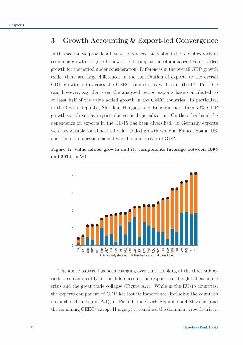
In this section we provide a first set of stylized facts about the role of exports in
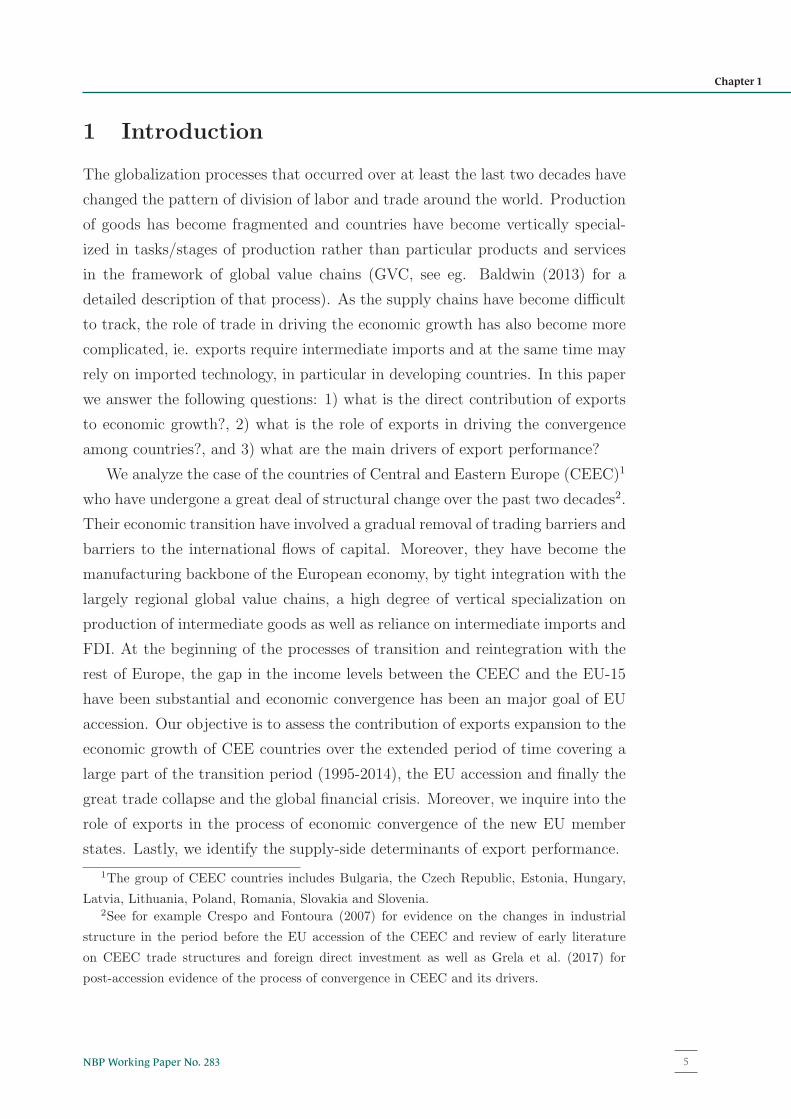
economic growth. Figure 1 shows the decomposition of annualized value added
growth for the period under consideration. Differences in the overall GDP growth
aside, there are large differences in the contribution of exports to the overall
GDP growth both across the CEEC countries as well as in the EU-15. One
can, however, say that over the analyzed period exports have contributed to
at least half of the value added growth in the CEEC countries. In particular,
in the Czech Republic, Slovakia, Hungary and Bulgaria more than 70% GDP
growth was driven by exports due vertical specialization. On the other hand the
dependence on exports in the EU-15 has been diversified. In Germany exports
were responsible for almost all value added growth while in France, Spain, UK
and Finland domestic demand was the main driver of GDP.
Figure 1: Value added growth and its components (average between 1995
and 2014, in %)
0
1
2
3
4
IT
A
GR
C
DN
K
PR
T
DE
U
FR
A
AU
T
BE
L
CZ
E
FIN
NL
D
ES
P
GB
R
HU
N
CY
P
SW
E
RO
U
SV
N
IR
L
BG
R
SV
K
LU
X
LV
A
PO
L
ES
T
LT
U
Domestically absorbed Absorbed abroad Value Added
The above pattern has been changing over time. Looking at the three subpe-
riods, one can identify major differences in the response to the global economic
crisis and the great trade collapse (Figure A.1). While in the EU-15 countries,
the exports component of GDP has lost its importance (including the countries
not included in Figure A.1), in Poland, the Czech Republic and Slovakia (and
10
3 Growth Accounting & Export-led Convergence
In this section we provide a first set of stylized facts about the role of exports in
economic growth. Figure 1 shows the decomposition of annualized value added
growth for the period under consideration. Differences in the overall GDP growth
aside, there are large differences in the contribution of exports to the overall
GDP growth both across the CEEC countries as well as in the EU-15. One
can, however, say that over the analyzed period exports have contributed to
at least half of the value added growth in the CEEC countries. In particular,
in the Czech Republic, Slovakia, Hungary and Bulgaria more than 70% GDP
growth was driven by exports due vertical specialization. On the other hand the
dependence on exports in the EU-15 has been diversified. In Germany exports
were responsible for almost all value added growth while in France, Spain, UK
and Finland domestic demand was the main driver of GDP.
Figure 1: Value added growth and its components (average between 1995
and 2014, in %)
0
1
2
3
4
IT
A
GR
C
DN
K
PR
T
DE
U
FR
A
AU
T
BE
L
CZ
E
FIN
NL
D
ES
P
GB
R
HU
N
CY
P
SW
E
RO
U
SV
N
IR
L
BG
R
SV
K
LU
X
LV
A
PO
L
ES
T
LT
U
Domestically absorbed Absorbed abroad Value Added
The above pattern has been changing over time. Looking at the three subpe-
riods, one can identify major differences in the response to the global economic
crisis and the great trade collapse (Figure A.1). While in the EU-15 countries,
the exports component of GDP has lost its importance (including the countries
not included in Figure A.1), in Poland, the Czech Republic and Slovakia (and
10
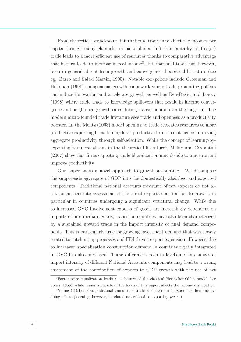
the remaining CEECs except Hungary) it remained the dominant growth driver.
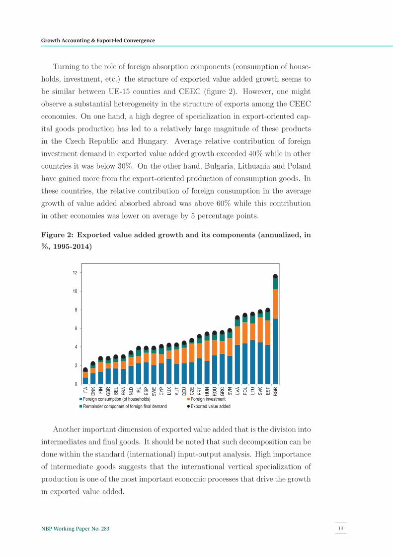
Turning to the role of foreign absorption components (consumption of house-
holds, investment, etc.) the structure of exported value added growth seems to
be similar between UE-15 counties and CEEC (figure 2). However, one might
observe a substantial heterogeneity in the structure of exports among the CEEC
economies. On one hand, a high degree of specialization in export-oriented cap-
ital goods production has led to a relatively large magnitude of these products
in the Czech Republic and Hungary. Average relative contribution of foreign
investment demand in exported value added growth exceeded 40% while in other
countries it was below 30%. On the other hand, Bulgaria, Lithuania and Poland
have gained more from the export-oriented production of consumption goods. In
these countries, the relative contribution of foreign consumption in the average
growth of value added absorbed abroad was above 60% while this contribution
in other economies was lower on average by 5 percentage points.
Figure 2: Exported value added growth and its components (annualized, in
%, 1995-2014)
0
2
4
6
8
10
12
ITA
DNK
FIN
GBR
BEL
FRA
NLD
IRL
ESP
SWE
CYP
LUX
AUT
DEU
CZE
PRT
HUN
ROU
GRC
SVN
LVA
POL
LTU
SVK
EST
BGR
Foreign consumption (of households) Foreign investment
Remainder component of foreign final demand Exported value added
Another important dimension of exported value added that is the division into
intermediates and final goods. It should be noted that such decomposition can be
done within the standard (international) input-output analysis. High importance
of intermediate goods suggests that the international vertical specialization of
production is one of the most important economic processes that drive the growth
11
Narodowy Bank Polski12
Chapter 3
the remaining CEECs except Hungary) it remained the dominant growth driver.
Turning to the role of foreign absorption components (consumption of house-
holds, investment, etc.) the structure of exported value added growth seems to
be similar between UE-15 counties and CEEC (figure 2). However, one might
observe a substantial heterogeneity in the structure of exports among the CEEC
economies. On one hand, a high degree of specialization in export-oriented cap-
ital goods production has led to a relatively large magnitude of these products
in the Czech Republic and Hungary. Average relative contribution of foreign
investment demand in exported value added growth exceeded 40% while in other
countries it was below 30%. On the other hand, Bulgaria, Lithuania and Poland
have gained more from the export-oriented production of consumption goods. In
these countries, the relative contribution of foreign consumption in the average
growth of value added absorbed abroad was above 60% while this contribution
in other economies was lower on average by 5 percentage points.
Figure 2: Exported value added growth and its components (annualized, in
%, 1995-2014)
0
2
4
6
8
10
12
ITA
DNK
FIN
GBR
BEL
FRA
NLD
IRL
ESP
SWE
CYP
LUX
AUT
DEU
CZE
PRT
HUN
ROU
GRC
SVN
LVA
POL
LTU
SVK
EST
BGR
Foreign consumption (of households) Foreign investment
Remainder component of foreign final demand Exported value added
Another important dimension of exported value added that is the division into
intermediates and final goods. It should be noted that such decomposition can be
done within the standard (international) input-output analysis. High importance
of intermediate goods suggests that the international vertical specialization of
production is one of the most important economic processes that drive the growth
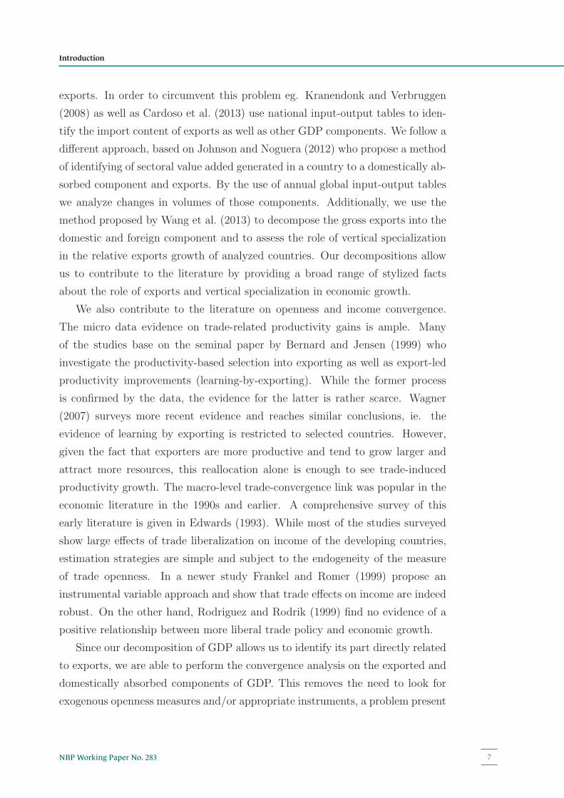
11in exported value added.
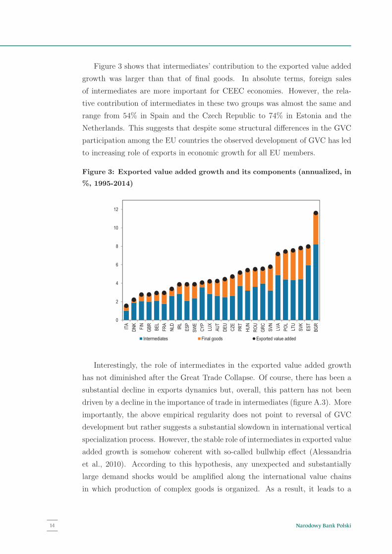
Figure 3 shows that intermediates’ contribution to the exported value added
growth was larger than that of final goods. In absolute terms, foreign sales
of intermediates are more important for CEEC economies. However, the rela-
tive contribution of intermediates in these two groups was almost the same and
range from 54% in Spain and the Czech Republic to 74% in Estonia and the
Netherlands. This suggests that despite some structural differences in the GVC
participation among the EU countries the observed development of GVC has led
to increasing role of exports in economic growth for all EU members.
Figure 3: Exported value added growth and its components (annualized, in
%, 1995-2014)
0
2
4
6
8
10
12
ITA
DNK
FIN
GBR
BEL
FRA
NLD
IRL
ESP
SWE
CYP
LUX
AUT
DEU
CZE
PRT
HUN
ROU
GRC
SVN
LVA
POL
LTU
SVK
EST
BGR
Intermediates Final goods Exported value added
Interestingly, the role of intermediates in the exported value added growth
has not diminished after the Great Trade Collapse. Of course, there has been a
substantial decline in exports dynamics but, overall, this pattern has not been
driven by a decline in the importance of trade in intermediates (figure A.3). More
importantly, the above empirical regularity does not point to reversal of GVC
development but rather suggests a substantial slowdown in international vertical
specialization process. However, the stable role of intermediates in exported value
added growth is somehow coherent with so-called bullwhip effect (Alessandria
et al., 2010). According to this hypothesis, any unexpected and substantially
large demand shocks would be amplified along the international value chains
12
13NBP Working Paper No. 283
Growth Accounting & Export-led Convergence
in exported value added.
Figure 3 shows that intermediates’ contribution to the exported value added
growth was larger than that of final goods. In absolute terms, foreign sales
of intermediates are more important for CEEC economies. However, the rela-
tive contribution of intermediates in these two groups was almost the same and
range from 54% in Spain and the Czech Republic to 74% in Estonia and the
Netherlands. This suggests that despite some structural differences in the GVC
participation among the EU countries the observed development of GVC has led
to increasing role of exports in economic growth for all EU members.
Figure 3: Exported value added growth and its components (annualized, in
%, 1995-2014)
0
2
4
6
8
10
12
ITA
DNK
FIN
GBR
BEL
FRA
NLD
IRL
ESP
SWE
CYP
LUX
AUT
DEU
CZE
PRT
HUN
ROU
GRC
SVN
LVA
POL
LTU
SVK
EST
BGR
Intermediates Final goods Exported value added
Interestingly, the role of intermediates in the exported value added growth
has not diminished after the Great Trade Collapse. Of course, there has been a
substantial decline in exports dynamics but, overall, this pattern has not been
driven by a decline in the importance of trade in intermediates (figure A.3). More
importantly, the above empirical regularity does not point to reversal of GVC
development but rather suggests a substantial slowdown in international vertical
specialization process. However, the stable role of intermediates in exported value
added growth is somehow coherent with so-called bullwhip effect (Alessandria
et al., 2010). According to this hypothesis, any unexpected and substantially
large demand shocks would be amplified along the international value chains
12in which production of complex goods is organized. As a result, it leads to a
disproportionate reaction of international trade. Although this mechanism is
widely employed to understand the Great Trade Collapse it can also explain
recovery of international trade after this period.
To scrutinize the importance of vertical specialization in economic growth
we extend the growth decomposition by identifying the structural change com-
ponent. Denoting t as time index, the intertemporal change in aggregate value
added of given economy (ΔyD→.t ) can be expressed as follows:
ΔyD→.t =
∑j∈{D,F}
∑i∈D
[L−1
t−1Δyjt
]i+
∑j∈{D,F}
∑i∈D
[(ΔL−1
t
)yjt−1
]i, (4)
where the first component measures the aggregate change in value added that ab-
stracts from shifts in production structure while the latter one captures structural
effects which refer to changes in output-input structure (intersectoral linkages)
of global economy.5 Both components can be divided into subcomponents of
domestically and foreign-absorbed value added. Intuitively, substantial contri-
bution of the second component highlights the role of gains or losses from vertical
specialization for economic growth.
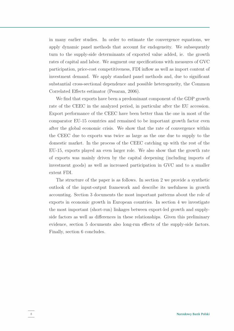
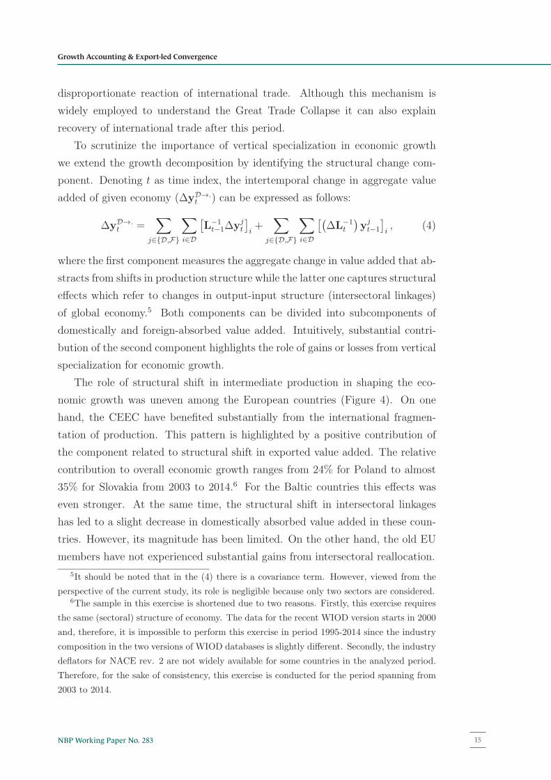
The role of structural shift in intermediate production in shaping the eco-
nomic growth was uneven among the European countries (Figure 4). On one
hand, the CEEC have benefited substantially from the international fragmen-
tation of production. This pattern is highlighted by a positive contribution of
the component related to structural shift in exported value added. The relative
contribution to overall economic growth ranges from 24% for Poland to almost
35% for Slovakia from 2003 to 2014.6 For the Baltic countries this effects was
even stronger. At the same time, the structural shift in intersectoral linkages
has led to a slight decrease in domestically absorbed value added in these coun-
tries. However, its magnitude has been limited. On the other hand, the old EU
5It should be noted that in the (4) there is a covariance term. However, viewed from the
perspective of the current study, its role is negligible because only two sectors are considered.6The sample in this exercise is shortened due to two reasons. Firstly, this exercise requires
the same (sectoral) structure of economy. The data for the recent WIOD version starts in 2000
and, therefore, it is impossible to perform this exercise in period 1995-2014 since the industry
composition in the two versions of WIOD databases is slightly different. Secondly, the industry
deflators for NACE rev. 2 are not widely available for some countries in the analyzed period.
Therefore, for the sake of consistency, this exercise is conducted for the period spanning from
2003 to 2014.
13
Narodowy Bank Polski14
in which production of complex goods is organized. As a result, it leads to a
disproportionate reaction of international trade. Although this mechanism is
widely employed to understand the Great Trade Collapse it can also explain
recovery of international trade after this period.
To scrutinize the importance of vertical specialization in economic growth
we extend the growth decomposition by identifying the structural change com-
ponent. Denoting t as time index, the intertemporal change in aggregate value
added of given economy (ΔyD→.t ) can be expressed as follows:
ΔyD→.t =
∑j∈{D,F}
∑i∈D
[L−1
t−1Δyjt
]i+
∑j∈{D,F}
∑i∈D
[(ΔL−1
t
)yjt−1
]i, (4)
where the first component measures the aggregate change in value added that ab-
stracts from shifts in production structure while the latter one captures structural
effects which refer to changes in output-input structure (intersectoral linkages)
of global economy.5 Both components can be divided into subcomponents of
domestically and foreign-absorbed value added. Intuitively, substantial contri-
bution of the second component highlights the role of gains or losses from vertical
specialization for economic growth.
The role of structural shift in intermediate production in shaping the eco-
nomic growth was uneven among the European countries (Figure 4). On one
hand, the CEEC have benefited substantially from the international fragmen-
tation of production. This pattern is highlighted by a positive contribution of
the component related to structural shift in exported value added. The relative
contribution to overall economic growth ranges from 24% for Poland to almost
35% for Slovakia from 2003 to 2014.6 For the Baltic countries this effects was
even stronger. At the same time, the structural shift in intersectoral linkages
has led to a slight decrease in domestically absorbed value added in these coun-
tries. However, its magnitude has been limited. On the other hand, the old EU
5It should be noted that in the (4) there is a covariance term. However, viewed from the
perspective of the current study, its role is negligible because only two sectors are considered.6The sample in this exercise is shortened due to two reasons. Firstly, this exercise requires
the same (sectoral) structure of economy. The data for the recent WIOD version starts in 2000
and, therefore, it is impossible to perform this exercise in period 1995-2014 since the industry
composition in the two versions of WIOD databases is slightly different. Secondly, the industry
deflators for NACE rev. 2 are not widely available for some countries in the analyzed period.
Therefore, for the sake of consistency, this exercise is conducted for the period spanning from
2003 to 2014.
13
members have not experienced substantial gains from intersectoral reallocation.
Figure 4: GDP growth and its components (annualized, in %, 2003-2014)
-3
-2
-1
0
1
2
3
4
GR
C
IT
A
PR
T
HR
V
FIN
DN
K
IR
L
ES
P
HU
N
CY
P
FR
A
DE
U
NLD
AU
T
SV
N
BE
L
GB
R
SW
E
CZ
E
CH
E
LV
A
ES
T
LU
X
BG
R
RO
U
LT
U
SV
K
PO
L
(Purely) domestically absorbed (Purely) absorbed abroad (Structural) domestically absorbed
(Structural) absorbed abroad Value Added
Intuitively, the systematic differences in economic performance between CEEC
and non-CEEC countries fueled the catching-up process. At the same, the above
documented empirical regularities suggest that the exported value added played
a crucial role in overall economic growth of European countries. To assess the ris-
ing role of exports in the catching-up process we use the standard (unconditional)
convergence equation (Durlauf et al., 2005):
Δyit = β0 − βCyit−1 + εit, (5)
where Δyit and yit−1 represent the dynamics and the logged lagged level of the
value added PPP per capita (vaPPPit ) or its specific part, i.e., domestically ab-
sorbed (dvaPPPit ) or exported component (evaPPP
it ). In the above formulation,
the parameter βC is the convergence rate and it measures the speed of (uncon-
ditional) catching-up process. If the convergence equation (5) is applied to the
cross-sectional data then Δyit denotes the average growth rate over period and
yit−1 is the initial level.
We subsequently look into the patterns of convergence across our sample.
Figure 5 shows the 1995 log levels of value added and its two components per
capita in PPP7 versus the average real growth rate of those components over
7The series on data on purchasing power parity are taken from Eurostat while series on
14
15NBP Working Paper No. 283
Growth Accounting & Export-led Convergence
members have not experienced substantial gains from intersectoral reallocation.
Figure 4: GDP growth and its components (annualized, in %, 2003-2014)
-3
-2
-1
0
1
2
3
4
GR
C
IT
A
PR
T
HR
V
FIN
DN
K
IR
L
ES
P
HU
N
CY
P
FR
A
DE
U
NLD
AU
T
SV
N
BE
L
GB
R
SW
E
CZ
E
CH
E
LV
A
ES
T
LU
X
BG
R
RO
U
LT
U
SV
K
PO
L
(Purely) domestically absorbed (Purely) absorbed abroad (Structural) domestically absorbed
(Structural) absorbed abroad Value Added
Intuitively, the systematic differences in economic performance between CEEC
and non-CEEC countries fueled the catching-up process. At the same, the above
documented empirical regularities suggest that the exported value added played
a crucial role in overall economic growth of European countries. To assess the ris-
ing role of exports in the catching-up process we use the standard (unconditional)
convergence equation (Durlauf et al., 2005):
Δyit = β0 − βCyit−1 + εit, (5)
where Δyit and yit−1 represent the dynamics and the logged lagged level of the
value added PPP per capita (vaPPPit ) or its specific part, i.e., domestically ab-
sorbed (dvaPPPit ) or exported component (evaPPP
it ). In the above formulation,
the parameter βC is the convergence rate and it measures the speed of (uncon-
ditional) catching-up process. If the convergence equation (5) is applied to the
cross-sectional data then Δyit denotes the average growth rate over period and
yit−1 is the initial level.
We subsequently look into the patterns of convergence across our sample.
Figure 5 shows the 1995 log levels of value added and its two components per
capita in PPP7 versus the average real growth rate of those components over
7The series on data on purchasing power parity are taken from Eurostat while series on
14
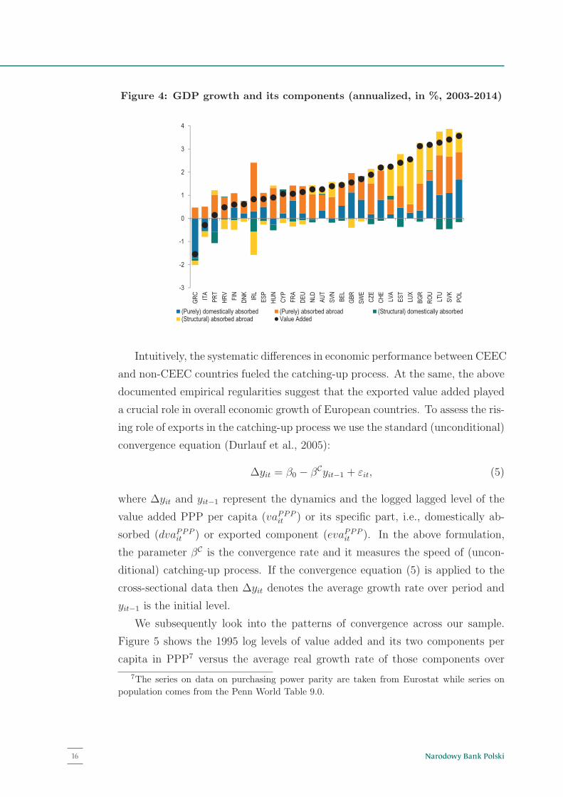
Figure 5: The growth rate of value added (vertical axis) and the logged
value added PPP per capita (horizontal axis)
AUTBEL
BGR
CYP
CZE
DEU
DNK
ESP
EST
FIN
FRA
GBR
GRC
HUN
IRL
ITA
LTU
LUX
LVA
NLD
POL
PRT
ROU SVK
SVN
SWE
BGR
CZE
EST
HUN
LTU
LVA
POL
ROU SVK
SVN
0.01
.02
.03
.04
.05
4 4.5 5 5.5 6
AUTBEL
BGR
CYPCZE DEUDNK
ESP
EST
FIN
FRA
GBR
GRC
HUN
IRLITA
LTU
LUX
LVA
NLD
POL
PRT
ROU
SVK
SVN
SWEBGR
CZE
EST
HUN
LTULVA
POL
ROU
SVK
SVN
0.01
.02
.03
.04
4 4.5 5 5.5
AUT
BEL
BGR
CYP
CZEDEU
DNK
ESP
EST
FINFRAGBR
GRCHUN
IRL
ITA
LTU
LUX
LVA
NLD
POL
PRT
ROU
SVK
SVN
SWE
BGR
CZE
EST
HUN
LTULVA
POL
ROU
SVK
SVN
.02
.04
.06
.08
.1.12
1 2 3 4 5 6
Note: Left: total value added, center: domestically absorbed value added, right: exported
value added. Red and blue color refers to CEEC and non-CEEC countries, respectively.
the analyzed period. This preliminary analysis shows a somewhat clear pattern
of convergence (negative slope) across the analyzed countries both in terms of
total value added as well as exported value added. The domestically absorbed
value added convergence seems to be a phenomenon present in the CEEC group
while the negative growth-level relationship in the non-CEEC countries is less
evident. Our visual inspection is confirmed with the cross-section regression
results. Namely, in the analyzed sample, i.e., from 1995 to 2014, the estimated
pace of convergence in GDP is consistent with the literature consensus and equals
2.1%. The catching-up parameters βC for the domestically absorbed and exported
value added are around 1.7% and 2.5%, respectively.
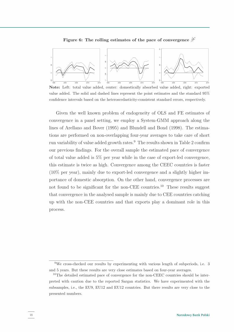
Figure 6 shows the one year rolling estimates of cross-section regressions of
value added component growth rates on the lagged log-levels. Looking at time
variation the levels of the estimated convergence coefficient (in absolute terms)
are on average visibly higher in the case of exported value added than in the
case of the domestically absorbed value added. Naturally, in the case of total
value added this implies a higher contribution of exports rather than domestic
absorption to overall convergence. This export-led convergence has not been,
however, uniform over time. While the late 1990s have seen the Asian and,
more importantly, the Russian crisis that have negatively affected exports in the
CEE, the pace of export-led convergence picked-up in the pre-accession period
after 2000 (when most of trade barriers in the CEE-EU trade had already been
eliminated8), and intensified after the EU enlargements in 2004 and 2007 with an
eventual slowdown during the global financial crisis of 2009 and sluggish recovery
population comes from the Penn World Table 9.0.8except the agricultural and food sector.
15
Narodowy Bank Polski16
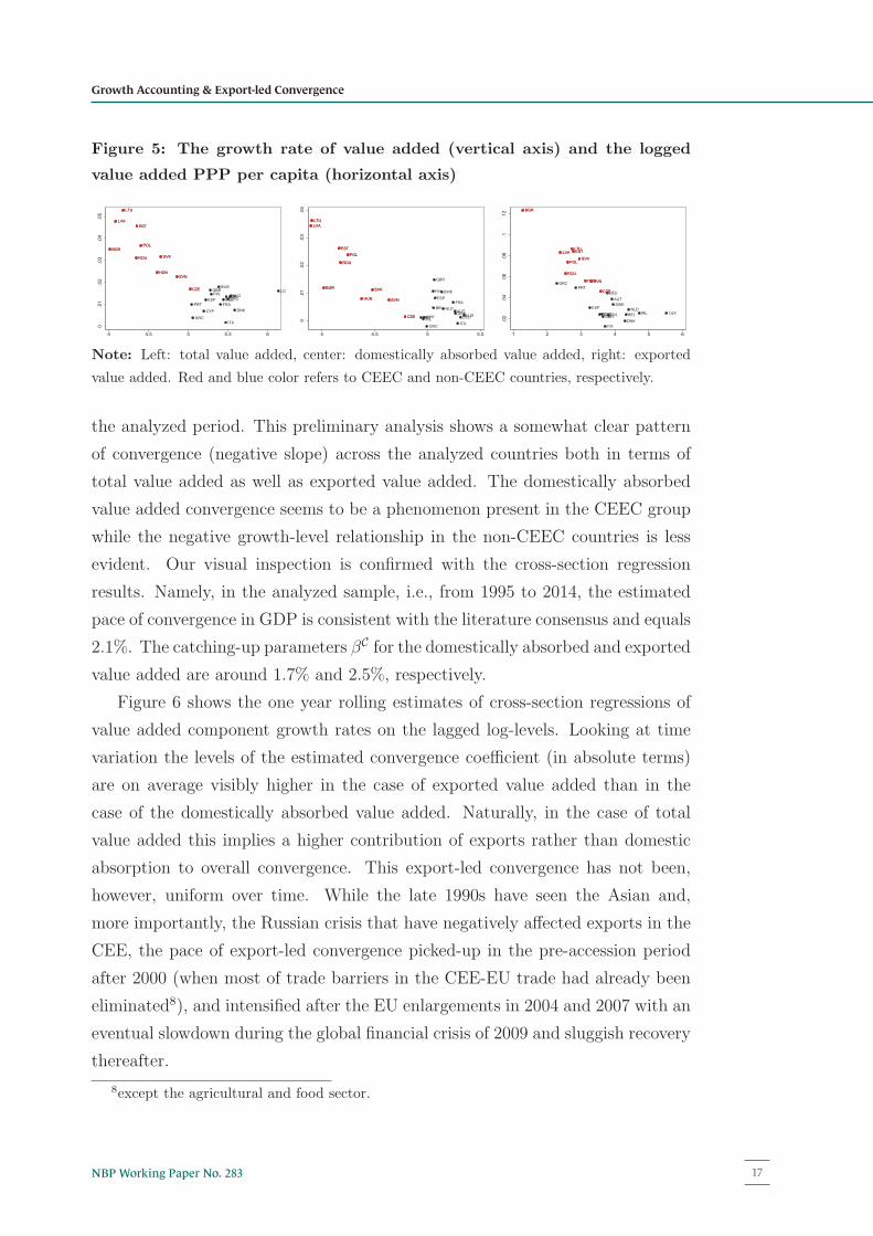
Figure 5: The growth rate of value added (vertical axis) and the logged
value added PPP per capita (horizontal axis)
AUTBEL
BGR
CYP
CZE
DEU
DNK
ESP
EST
FIN
FRA
GBR
GRC
HUN
IRL
ITA
LTU
LUX
LVA
NLD
POL
PRT
ROU SVK
SVN
SWE
BGR
CZE
EST
HUN
LTU
LVA
POL
ROU SVK
SVN
0.01
.02
.03
.04
.05
4 4.5 5 5.5 6
AUTBEL
BGR
CYPCZE DEUDNK
ESP
EST
FIN
FRA
GBR
GRC
HUN
IRLITA
LTU
LUX
LVA
NLD
POL
PRT
ROU
SVK
SVN
SWEBGR
CZE
EST
HUN
LTULVA
POL
ROU
SVK
SVN0
.01
.02
.03
.04
4 4.5 5 5.5
AUT
BEL
BGR
CYP
CZEDEU
DNK
ESP
EST
FINFRAGBR
GRCHUN
IRL
ITA
LTU
LUX
LVA
NLD
POL
PRT
ROU
SVK
SVN
SWE
BGR
CZE
EST
HUN
LTULVA
POL
ROU
SVK
SVN
.02
.04
.06
.08
.1.12
1 2 3 4 5 6
Note: Left: total value added, center: domestically absorbed value added, right: exported
value added. Red and blue color refers to CEEC and non-CEEC countries, respectively.
the analyzed period. This preliminary analysis shows a somewhat clear pattern
of convergence (negative slope) across the analyzed countries both in terms of
total value added as well as exported value added. The domestically absorbed
value added convergence seems to be a phenomenon present in the CEEC group
while the negative growth-level relationship in the non-CEEC countries is less
evident. Our visual inspection is confirmed with the cross-section regression
results. Namely, in the analyzed sample, i.e., from 1995 to 2014, the estimated
pace of convergence in GDP is consistent with the literature consensus and equals
2.1%. The catching-up parameters βC for the domestically absorbed and exported
value added are around 1.7% and 2.5%, respectively.
Figure 6 shows the one year rolling estimates of cross-section regressions of
value added component growth rates on the lagged log-levels. Looking at time
variation the levels of the estimated convergence coefficient (in absolute terms)
are on average visibly higher in the case of exported value added than in the
case of the domestically absorbed value added. Naturally, in the case of total
value added this implies a higher contribution of exports rather than domestic
absorption to overall convergence. This export-led convergence has not been,
however, uniform over time. While the late 1990s have seen the Asian and,
more importantly, the Russian crisis that have negatively affected exports in the
CEE, the pace of export-led convergence picked-up in the pre-accession period
after 2000 (when most of trade barriers in the CEE-EU trade had already been
eliminated8), and intensified after the EU enlargements in 2004 and 2007 with an
eventual slowdown during the global financial crisis of 2009 and sluggish recovery
population comes from the Penn World Table 9.0.8except the agricultural and food sector.
15
Figure 5: The growth rate of value added (vertical axis) and the logged
value added PPP per capita (horizontal axis)
AUTBEL
BGR
CYP
CZE
DEU
DNK
ESP
EST
FIN
FRA
GBR
GRC
HUN
IRL
ITA
LTU
LUX
LVA
NLD
POL
PRT
ROU SVK
SVN
SWE
BGR
CZE
EST
HUN
LTU
LVA
POL
ROU SVK
SVN
0.01
.02
.03
.04
.05
4 4.5 5 5.5 6
AUTBEL
BGR
CYPCZE DEUDNK
ESP
EST
FIN
FRA
GBR
GRC
HUN
IRLITA
LTU
LUX
LVA
NLD
POL
PRT
ROU
SVK
SVN
SWEBGR
CZE
EST
HUN
LTULVA
POL
ROU
SVK
SVN
0.01
.02
.03
.04
4 4.5 5 5.5
AUT
BEL
BGR
CYP
CZEDEU
DNK
ESP
EST
FINFRAGBR
GRCHUN
IRL
ITA
LTU
LUX
LVA
NLD
POL
PRT
ROU
SVK
SVN
SWE
BGR
CZE
EST
HUN
LTULVA
POL
ROU
SVK
SVN
.02
.04
.06
.08
.1.12
1 2 3 4 5 6
Note: Left: total value added, center: domestically absorbed value added, right: exported
value added. Red and blue color refers to CEEC and non-CEEC countries, respectively.
the analyzed period. This preliminary analysis shows a somewhat clear pattern
of convergence (negative slope) across the analyzed countries both in terms of
total value added as well as exported value added. The domestically absorbed
value added convergence seems to be a phenomenon present in the CEEC group
while the negative growth-level relationship in the non-CEEC countries is less
evident. Our visual inspection is confirmed with the cross-section regression
results. Namely, in the analyzed sample, i.e., from 1995 to 2014, the estimated
pace of convergence in GDP is consistent with the literature consensus and equals
2.1%. The catching-up parameters βC for the domestically absorbed and exported
value added are around 1.7% and 2.5%, respectively.
Figure 6 shows the one year rolling estimates of cross-section regressions of
value added component growth rates on the lagged log-levels. Looking at time
variation the levels of the estimated convergence coefficient (in absolute terms)
are on average visibly higher in the case of exported value added than in the
case of the domestically absorbed value added. Naturally, in the case of total
value added this implies a higher contribution of exports rather than domestic
absorption to overall convergence. This export-led convergence has not been,
however, uniform over time. While the late 1990s have seen the Asian and,
more importantly, the Russian crisis that have negatively affected exports in the
CEE, the pace of export-led convergence picked-up in the pre-accession period
after 2000 (when most of trade barriers in the CEE-EU trade had already been
eliminated8), and intensified after the EU enlargements in 2004 and 2007 with an
eventual slowdown during the global financial crisis of 2009 and sluggish recovery
population comes from the Penn World Table 9.0.8except the agricultural and food sector.
15
thereafter.
Figure 6: The rolling estimates of the pace of convergence βC
-.05
0.05
.1
1995 2000 2005 2010 2015
-.1-.05
0.05
.1
1995 2000 2005 2010 2015
-.05
0.05
.1.15
1995 2000 2005 2010 2015
Note: Left: total value added, center: domestically absorbed value added, right: exported
value added. The solid and dashed lines represent the point estimates and the standard 95%
confidence intervals based on the heteroscedasticity-consistent standard errors, respectively.
Given the well known problem of endogeneity of OLS and FE estimates of
convergence in a panel setting, we employ a System-GMM approach along the
lines of Arellano and Bover (1995) and Blundell and Bond (1998). The estima-
tions are performed on non-overlapping four-year averages to take care of short
run variability of value added growth rates.9 The results shown in Table 2 confirm
our previous findings. For the overall sample the estimated pace of convergence
of total value added is 5% per year while in the case of export-led convergence,
this estimate is twice as high. Convergence among the CEEC countries is faster
(10% per year), mainly due to export-led convergence and a slightly higher im-
portance of domestic absorption. On the other hand, convergence processes are
not found to be significant for the non-CEE countries.10 These results suggest
that convergence in the analysed sample is mainly due to CEE countries catching
up with the non-CEE countries and that exports play a dominant role in this
process.
9We cross-checked our results by experimenting with various length of subperiods, i.e. 3
and 5 years. But these results are very close estimates based on four-year averages.10The detailed estimated pace of convergence for the non-CEEC countries should be inter-
preted with caution due to the reported Sargan statistics. We have experimented with the
subsamples, i.e., the EU9, EU12 and EU12 countries. But there results are very close to the
presented numbers.
16
17NBP Working Paper No. 283
Growth Accounting & Export-led Convergence
thereafter.
Figure 6: The rolling estimates of the pace of convergence βC
-.05
0.05
.1
1995 2000 2005 2010 2015
-.1-.05
0.05
.1
1995 2000 2005 2010 2015
-.05
0.05
.1.15
1995 2000 2005 2010 2015
Note: Left: total value added, center: domestically absorbed value added, right: exported
value added. The solid and dashed lines represent the point estimates and the standard 95%
confidence intervals based on the heteroscedasticity-consistent standard errors, respectively.
Given the well known problem of endogeneity of OLS and FE estimates of
convergence in a panel setting, we employ a System-GMM approach along the
lines of Arellano and Bover (1995) and Blundell and Bond (1998). The estima-
tions are performed on non-overlapping four-year averages to take care of short
run variability of value added growth rates.9 The results shown in Table 2 confirm
our previous findings. For the overall sample the estimated pace of convergence
of total value added is 5% per year while in the case of export-led convergence,
this estimate is twice as high. Convergence among the CEEC countries is faster
(10% per year), mainly due to export-led convergence and a slightly higher im-
portance of domestic absorption. On the other hand, convergence processes are
not found to be significant for the non-CEE countries.10 These results suggest
that convergence in the analysed sample is mainly due to CEE countries catching
up with the non-CEE countries and that exports play a dominant role in this
process.
9We cross-checked our results by experimenting with various length of subperiods, i.e. 3
and 5 years. But these results are very close estimates based on four-year averages.10The detailed estimated pace of convergence for the non-CEEC countries should be inter-
preted with caution due to the reported Sargan statistics. We have experimented with the
subsamples, i.e., the EU9, EU12 and EU12 countries. But there results are very close to the
presented numbers.
16
thereafter.
Figure 6: The rolling estimates of the pace of convergence βC-.05
0.05
.1
1995 2000 2005 2010 2015
-.1-.05
0.05
.1
1995 2000 2005 2010 2015
-.05
0.05
.1.15
1995 2000 2005 2010 2015
Note: Left: total value added, center: domestically absorbed value added, right: exported
value added. The solid and dashed lines represent the point estimates and the standard 95%
confidence intervals based on the heteroscedasticity-consistent standard errors, respectively.
Given the well known problem of endogeneity of OLS and FE estimates of
convergence in a panel setting, we employ a System-GMM approach along the
lines of Arellano and Bover (1995) and Blundell and Bond (1998). The estima-
tions are performed on non-overlapping four-year averages to take care of short
run variability of value added growth rates.9 The results shown in Table 2 confirm
our previous findings. For the overall sample the estimated pace of convergence
of total value added is 5% per year while in the case of export-led convergence,
this estimate is twice as high. Convergence among the CEEC countries is faster
(10% per year), mainly due to export-led convergence and a slightly higher im-
portance of domestic absorption. On the other hand, convergence processes are
not found to be significant for the non-CEE countries.10 These results suggest
that convergence in the analysed sample is mainly due to CEE countries catching
up with the non-CEE countries and that exports play a dominant role in this
process.
9We cross-checked our results by experimenting with various length of subperiods, i.e. 3
and 5 years. But these results are very close estimates based on four-year averages.10The detailed estimated pace of convergence for the non-CEEC countries should be inter-
preted with caution due to the reported Sargan statistics. We have experimented with the
subsamples, i.e., the EU9, EU12 and EU12 countries. But there results are very close to the
presented numbers.
16
Narodowy Bank Polski18
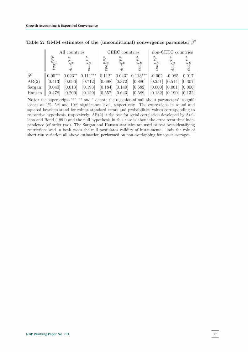
Table 2: GMM estimates of the (unconditional) convergence parameter βC
All countries CEEC countries non-CEEC countriestvaPPP
it
dvaPPP
it
evaPPP
it
tvaPPP
it
dvaPPP
it
evaPPP
it
tvaPPP
it
dvaPPP
it
evaPPP
it
βC 0.05∗∗∗ 0.023∗∗ 0.111∗∗∗ 0.112∗ 0.043∗ 0.113∗∗∗ -0.002 -0.085 0.017AR(2) [0.413] [0.096] [0.712] [0.698] [0.372] [0.880] [0.251] [0.514] [0.307]Sargan [0.040] [0.013] [0.193] [0.184] [0.149] [0.582] [0.000] [0.001] [0.000]Hansen [0.478] [0.200] [0.129] [0.557] [0.643] [0.589] [0.132] [0.190] [0.132]
Note: the superscripts ∗∗∗, ∗∗ and ∗ denote the rejection of null about parameters’ insignif-icance at 1%, 5% and 10% significance level, respectively. The expressions in round andsquared brackets stand for robust standard errors and probabilities values corresponding torespective hypothesis, respectively. AR(2) it the test for serial correlation developed by Arel-lano and Bond (1991) and the null hypothesis in this case is about the error term time inde-pendence (of order two). The Sargan and Hansen statistics are used to test over-identifyingrestrictions and in both cases the null postulates validity of instruments. limit the role ofshort-run variation all above estimation performed on non-overlapping four-year averages.
17
19NBP Working Paper No. 283
Growth Accounting & Export-led Convergence
4 Determinants of export-led growth
In this section we turn to the analysis of the determinants of export-led growth.
We combined the data on neoclassical factors of production, measures of ver-
tical specialization and price-cost competitiveness and FDI stocks. The detailed
description of variables is delegated to table A.1. The dataset consists of series
for 26 countries over 19 years. Table A.2 reports the measures of cross-sectional
dependence and the results of panel unit root tests. The formal test statistics
proposed by (Pesaran, 2015) are extremely high for all variables of interest and
their first differences. The null is about cross sectional independence and it is
easily rejected at any reasonable significance level. The identified cross-sectional
dependence is crucial for testing a unit root. Therefore, we use a broad range of
panel unit root test including the standard IPS test (Im et al., 2003) and statisti-
cal procedures that account for cross-sectional dependence proposed by Pesaran
(2007) and Chang (2002). Nevertheless, the results of all tests do not allow to re-
ject the null about a unit root for our variables (or their logs). First-differencing
renders all variables stationary.
Given above features of the data and our focus on supply-side factors our
starting point is the (logged) production function for the differenced variables:
Δyit = α0 + α1Δkit + α2Δlit + α3Δxit + εit, (6)
where Δyit ∈ {Δvait,Δdvait,Δevait}, kit and lit stands up for the logged capital
and labor input, respectively, xit denotes the additional independent variable and
εit is the error term.
We begin by running panel regressions of the total growth rate of value added,
growth rate of domestically absorbed value added and exported value added on
the supply side variables, namely the growth rates of capital and labor.
The results of those preliminary regressions are shown in Table 3 and they
point out to the importance of both the economic cycle as well as the unobserved
heterogeneity in growth rates of value added components. In particular, inclusion
of time dummies has a visible downward bearing on the estimates of labor of the
pooled regressions. The estimates of the capital elasticity in the case of the pooled
regressions are visibly higher for the exported value added while the estimates of
labor elasticity tend to be higher for the domestically absorbed value added.
Cross sectional heterogeneity is large. Inclusion of country fixed effects in-
flates almost all the estimated elasticities except the elasticity of capital on ex-
18
Narodowy Bank Polski20
Chapter 4
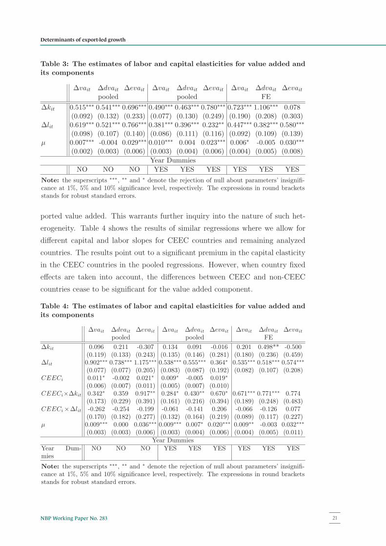
Table 3: The estimates of labor and capital elasticities for value added andits components
Δvait Δdvait Δevait Δvait Δdvait Δevait Δvait Δdvait Δevaitpooled pooled FE
Δkit 0.515∗∗∗ 0.541∗∗∗ 0.696∗∗∗ 0.490∗∗∗ 0.463∗∗∗ 0.780∗∗∗ 0.723∗∗∗ 1.106∗∗∗ 0.078(0.092) (0.132) (0.233) (0.077) (0.130) (0.249) (0.190) (0.208) (0.303)
Δlit 0.619∗∗∗ 0.521∗∗∗ 0.766∗∗∗ 0.381∗∗∗ 0.396∗∗∗ 0.232∗∗ 0.447∗∗∗ 0.382∗∗∗ 0.580∗∗∗
(0.098) (0.107) (0.140) (0.086) (0.111) (0.116) (0.092) (0.109) (0.139)μ 0.007∗∗∗ -0.004 0.029∗∗∗ 0.010∗∗∗ 0.004 0.023∗∗∗ 0.006∗ -0.005 0.030∗∗∗
(0.002) (0.003) (0.006) (0.003) (0.004) (0.006) (0.004) (0.005) (0.008)
Year Dummies
NO NO NO YES YES YES YES YES YES
Note: the superscripts ∗∗∗, ∗∗ and ∗ denote the rejection of null about parameters’ insignifi-cance at 1%, 5% and 10% significance level, respectively. The expressions in round bracketsstands for robust standard errors.
ported value added. This warrants further inquiry into the nature of such het-
erogeneity. Table 4 shows the results of similar regressions where we allow for
different capital and labor slopes for CEEC countries and remaining analyzed
countries. The results point out to a significant premium in the capital elasticity
in the CEEC countries in the pooled regressions. However, when country fixed
effects are taken into account, the differences between CEEC and non-CEEC
countries cease to be significant for the value added component.
Table 4: The estimates of labor and capital elasticities for value added andits components
Δvait Δdvait Δevait Δvait Δdvait Δevait Δvait Δdvait Δevaitpooled pooled FE
Δkit 0.096 0.211 -0.307 0.134 0.091 -0.016 0.201 0.498** -0.500(0.119) (0.133) (0.243) (0.135) (0.146) (0.281) (0.180) (0.236) (0.459)
Δlit 0.902∗∗∗ 0.738∗∗∗ 1.175∗∗∗ 0.538∗∗∗ 0.555∗∗∗ 0.364∗ 0.535∗∗∗ 0.518∗∗∗ 0.574∗∗∗
(0.077) (0.077) (0.205) (0.083) (0.087) (0.192) (0.082) (0.107) (0.208)CEECi 0.011∗ -0.002 0.021∗ 0.009∗ -0.005 0.019∗
(0.006) (0.007) (0.011) (0.005) (0.007) (0.010)CEECi×Δkit 0.342∗ 0.359 0.917∗∗ 0.284∗ 0.430∗∗ 0.670∗ 0.671∗∗∗ 0.771∗∗∗ 0.774
(0.173) (0.229) (0.391) (0.161) (0.216) (0.394) (0.189) (0.248) (0.483)CEECi×Δlit -0.262 -0.254 -0.199 -0.061 -0.141 0.206 -0.066 -0.126 0.077
(0.170) (0.182) (0.277) (0.132) (0.164) (0.219) (0.089) (0.117) (0.227)μ 0.009∗∗∗ 0.000 0.036∗∗∗ 0.009∗∗∗ 0.007∗ 0.020∗∗∗ 0.009∗∗ -0.003 0.032∗∗∗
(0.003) (0.003) (0.006) (0.003) (0.004) (0.006) (0.004) (0.005) (0.011)Year Dummies
Year Dum-mies
NO NO NO YES YES YES YES YES YES
Note: the superscripts ∗∗∗, ∗∗ and ∗ denote the rejection of null about parameters’ insignifi-cance at 1%, 5% and 10% significance level, respectively. The expressions in round bracketsstands for robust standard errors.
19
21NBP Working Paper No. 283
Determinants of export-led growth
In order to explore the within variation slightly further, we introduce addi-
tional control variables into our exported value added regressions. We control for
such export-related structural factors as the participation in global value chains
(foreign value added content of exports), the level of competitiveness measured
by real effective exchange rate based on ULC (unit labor costss), the stock of
inward FDI as well as the import intensity of investment to account for possible
technological spillovers from these two sources.
All of the additional controls (Table A.3) turn out to be important drivers of
exported value added growth. Moreover, for most of the analyzed variables, the
effect for the CEEC countries is significantly higher than for remaining countries.
This is in particular true for foreign value added content of exports where the
elasticity of exported value added growth in CEEC is almost double the one of the
non-CEEC countries. While FDI is only weakly affecting export capacity of the
CEEC countries, the effect of the import-intensity of investment is positive and
significant. These factors work toward increasing of the CEEC countries export
potential and speed up the convergence process to the non-CEEC countries. It
is also important to note, that introducing additional controls into the equation
renders the capital elasticity of exports significantly higher than for the remaining
countries, showing the importance of the capital accumulation in building of
export potential in the CEEC.
Given the systematic difference between CEEC and non-CEEC countries we
turn to more thorough exploration of panel heterogeneity.
20
Narodowy Bank Polski22
5 Heterogeneous panel data estimates
Our preliminary evidence exploits mostly the short-run variation of data. How-
ever, the the long-run effect might differ from the short-run reaction reported in
the previous section. Therefore, we turn to the analysis of the long-run effects
through the lens of an error correction model.
To estimate the long-run elasticities we use a panel error correction model
(ECM):
Δyit = α0,i+α1,iΔkit+α2,iΔlit+α3,iΔxit+φ0,iyit−1+φ1,ikit−1+φ2,ilit−1+φ3,ixit+εit,
(7)
where yit ∈ {vait, dvait, evait} , kit and lit stands for the nonstationary (logged)
capital and labor input, xit is the additional independent variable and εit is the
error term. In the above formulation we relax the assumption that all parameters
are homogeneous among considered countries. The parameters α1,i, α2,i and α3,i
measure the contemporaneous reaction of outcome variable to a change in factors
of production. If the coefficient φ1,i (on the yjit−1) lies between −1 and 0 then it
is a central value in the ECM model because it captures the pace of adjustment
toward a (long-run) equilibrium. The long-run multiplier can be obtained directly
from the estimates of the equation (7) and are equal to −φ1,i/φ0,i, −φ2,i/φ0,i and
−φ2,i/φ0,i for capital, labor and additional independent variable, respectively.
Finally, it should be mentioned that the above formulation of the ECM model
nests the specification considered in the previous section. Namely, if the error
correction mechanism is absent (φi,0 = φi,1 = φi,2 = φi,3 = 0 for all countries)
and the assumption of short-run coefficients homogeneity is satisfied then (7)
simplifies to (6).
We use the Common Correlated Effect (CCE) estimator proposed by Pesaran
(2006). A natural way to account for potential slope heterogeneity is to per-
form mean group estimation which is a simple arithmetic average of coefficients
estimated at the individual (country) level. However, in the presence of cross-
sectional dependence this strategy does not produce reliable estimates due to a
presence of multi-factor structure of the error term. Pesaran (2006) postulates to
augment the individual-specific regression by cross-sectional averages of depen-
dent and independent variables to account for the error multi-factor structure.
More recently, Chudik and Pesaran (2015) show that taking into account the
lagged dependent and explanatory variable is plausible strategy for controlling
21
23NBP Working Paper No. 283
Chapter 5
the effects of the unknown error multi-factor structure in the dynamic models.
We follow this approach, but due to small time dimension, the individual-specific
regression are extended additionally by the cross section averages of lagged de-
pendent variables (Δyit and yit−1). Given relatively small time dimension we
also pool the adjustment coefficient (φ0,i = φ0). This choice stems out from the
fact that we are interested in (possible) heterogeneity of long-run estimates and
an assumption on homogeneity of the long-run multipliers would be therefore
pointless.11 To check validity of this restriction we run the standard Hausman
test.
In the baseline specification, we include only neoclassical factors of produc-
tion, i.e., labor and capital. Table 5 summarizes the estimates of the ECM model
for the value added and its components. For the value added (vait) the estimates
of the long-run elasticities of capital and labor are positive and below unity. In
addition, their sum does not exceed unity and when we take into consideration
the variation of those estimates then the null hypothesis of constant returns to
scale is strongly rejected in favor of decreasing return to scale. However, the
statistical properties are rather problematic. Namely, the residuals exhibit mod-
erate cross-sectional dependence and the error correction term is not stationary.
To overcome this problem and account for a possible trend in total factor pro-
ductivity in the ECM model for the vait is extended by a linear (time) trend.
These estimates (the second column in table 5) suggest the higher role of capital
deepening and the estimated long-run elasticity on capital is above 0.7.
The results for the ECM model for domestically absorbed value added are
strikingly different. In the baseline model (without trend, third column in table
5) the estimated long-run elasticities of interest are relatively small (on capital)
or insignificant (on labor). Akin to the previous case, the statistical inference
is not plausible here due to possible unit root in the error correction and cross-
sectional dependence of the residuals. In the extended model (with a linear
trend) the statistical properties are more trustworthy and the long-run elasticity
of capital is slightly higher. However, the estimated coefficient on time trend
is negative at 10% significance level. This puzzling estimate can be explained
11In addition, we have also experimented with pooling other coefficients, i.e., various combi-
nation of φ0,i, α1,i, α2,i, α3,i and φ3,i. Although the qualitative implications remained almost
unchanged the Hausman statistics suggested that pooled estimates differ significantly from
their mean group counterparts in some cases.
22
Narodowy Bank Polski24
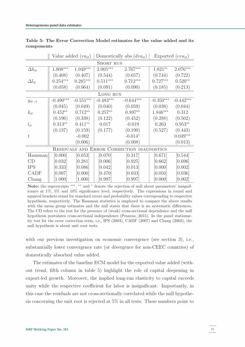
Table 5: The Error Correction Model estimates for the value added and itscomponents
Value added (vait) Domestically abs.(dvait) Exported (evait)
Short runΔkit 1.808∗∗∗ 1.949∗∗∗ 2.005∗∗∗ 2.767∗∗∗ 1.821∗∗ 2.076∗∗∗
(0.408) (0.407) (0.544) (0.657) (0.744) (0.722)Δlit 0.254∗∗∗ 0.285∗∗∗ 0.511∗∗∗ 0.712∗∗∗ 0.727∗∗∗ 0.520∗∗
(0.058) (0.064) (0.091) (0.090) (0.185) (0.213)
Long runyit−1 -0.490∗∗∗ -0.551∗∗∗ -0.483∗∗∗ -0.644∗∗∗ -0.350∗∗∗ -0.442∗∗∗
(0.045) (0.049) (0.040) (0.059) (0.038) (0.044)kit 0.452∗∗ 0.712∗∗ 0.257∗∗ 0.897∗∗ 1.846∗∗∗ 0.312
(0.196) (0.338) (0.122) (0.452) (0.288) (0.502)lit 0.313∗∗ 0.411∗∗ 0.017 -0.019 0.263 0.953∗∗
(0.137) (0.159) (0.177) (0.190) (0.527) (0.443)t -0.002 -0.014∗ 0.049∗∗∗
(0.006) (0.008) (0.013)
Residuals and Error Correction diagnosticsHausman [0.000] [0.053] [0.070] [0.317] [0.671] [0.544]CD [0.032] [0.281] [0.006] [0.925] [0.662] [0.696]IPS [0.333] [0.086] [0.042] [0.013] [0.000] [0.002]CADF [0.007] [0.000] [0.470] [0.033] [0.050] [0.036]Chang [1.000] [1.000] [0.997] [0.997] [0.000] [0.002]
Note: the superscripts ∗∗∗, ∗∗ and ∗ denote the rejection of null about parameters’ insignif-icance at 1%, 5% and 10% significance level, respectively. The expressions in round andsquared brackets stand for standard errors and probability values corresponding to respectivehypothesis, respectively. The Hausman statistics is employed to compare the above resultswith the mean group estimates and the null states that there is no systematic differences.The CD refers to the test for the presence of (weak) cross-sectional dependence and the nullhypothesis postulates cross-sectional independence (Pesaran, 2015). In the panel stationar-ity test for the error correction term, i.e., IPS (2003), CADF (2007) and Chang (2002), thenull hypothesis is about unit root tests.
with our previous investigation on economic convergence (see section 3), i.e.,
substantially lower convergence rate (or divergence for non-CEEC countries) of
domestically absorbed value added.
The estimates of the baseline ECM model for the exported value added (with-
out trend, fifth column in table 5) highlight the role of capital deepening in
export-led growth. Moreover, the implied long-run elasticity to capital exceeds
unity while the respective coefficient for labor is insignificant. Importantly, in
this case the residuals are not cross-sectionally correlated while the null hypothe-
sis concerning the unit root is rejected at 5% in all tests. These numbers point to
23
25NBP Working Paper No. 283
Heterogeneous panel data estimates
capital-intensity of export-led growth. However, in our supply-side focus the ex-
traordinarily high long-run elasticity to capital can be explained by the absence
of technological factors. Therefore, as in previous cases, the ECM model for the
evait is extended by a linear trend. It turns out that this modification completely
changes our results. Namely, it reduces the long-run elasticity of capital to zero,
producing average growth rate of technology progress exceeding 4.9% per annum
and relatively high coefficient on labor. Based on these estimates, the implied
explanation of export-led growth is purely technological.
To rationalize our set of estimates for exported value added the ECM model
is extended by supply-side factors that can possibly have a long-run effect on
export-led growth. Table 6 presents a broad set of estimates based on a replace-
ment of time trend by such factors. Let us start with the foreign content of
exports (FAXit) which measures degree of international fragmentation of pro-
duction. By including import content of gross exports in the ECM model the
capital elasticity substantially decreased. More importantly, the implied effect
of change in FAXit on the evait is positive both in the short and long run. This
highlights the importance of vertical specialization for export-led growth.
In addition, we also consider the ECM with FDI, real effective exchange rate
and import content of investment. In all cases we find a slight reduction in long-
run effect of capital intensity, however, less pronounced than in the ECM model
with the FAXit. The estimated long-run estimates are in line with the economic
intuition.
Eyeballing long-run estimates at the country level (figure A.6–A.7) several
patterns can be identified. Firstly, export-led growth is more sensitive to changes
in capital in CEEC. Secondly, the role of labor input in the creation of the
exported value added is larger in the non-CEEC countries. Thirdly, the long-run
effects of globalization and technical change are almost the same in the CEEC
and non-CEEC countries.
According to the estimates for all alternative specifications labor is a crucial
supply-side driver of exported value added only in the short-run. In all cases the
estimated long-run elasticities are insignificant. This suggests that the export-led
growth is not labor-intensive. However, our proxy of labor input, i.e., aggregate
hours, does not take into account on-going changes in labor composition. To
challenge this issue we additionally consider human capital index (hcit) as a
measure of labor composition. The estimated long-run elasticities of human
24
Narodowy Bank Polski26
capital (the last column in table A.7) are positive which suggests that, in contrary
to labor quantity, the improvement in labor quality can additionally explained
the export performance.12
Summing up, our empirical evidence suggests systematic differences in the im-
portance of factors of production between exported and domestically absorbed
value added. In particular, the long-run export-led growth can be explained
mostly by capital deepening enhanced by international fragmentation of produc-
tion.
12We have experimented with labor-quality adjusted input. Namely, instead of using separate
proxies of labor quantity and quality, we considered their product. However, these estimates
are very close to the estimates based only on aggregate hours as proxy of labor input. These
results are available upon request.
25
27NBP Working Paper No. 283
Heterogeneous panel data estimates
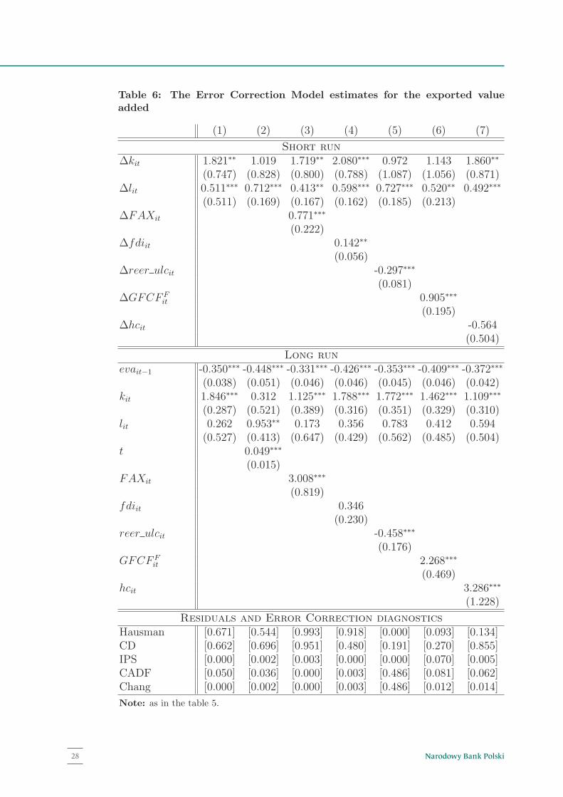
Table 6: The Error Correction Model estimates for the exported valueadded
(1) (2) (3) (4) (5) (6) (7)
Short runΔkit 1.821∗∗ 1.019 1.719∗∗ 2.080∗∗∗ 0.972 1.143 1.860∗∗
(0.747) (0.828) (0.800) (0.788) (1.087) (1.056) (0.871)Δlit 0.511∗∗∗ 0.712∗∗∗ 0.413∗∗ 0.598∗∗∗ 0.727∗∗∗ 0.520∗∗ 0.492∗∗∗
(0.511) (0.169) (0.167) (0.162) (0.185) (0.213)ΔFAXit 0.771∗∗∗
(0.222)Δfdiit 0.142∗∗
(0.056)Δreer ulcit -0.297∗∗∗
(0.081)ΔGFCF F
it 0.905∗∗∗
(0.195)Δhcit -0.564
(0.504)
Long runevait−1 -0.350∗∗∗ -0.448∗∗∗ -0.331∗∗∗ -0.426∗∗∗ -0.353∗∗∗ -0.409∗∗∗ -0.372∗∗∗
(0.038) (0.051) (0.046) (0.046) (0.045) (0.046) (0.042)kit 1.846∗∗∗ 0.312 1.125∗∗∗ 1.788∗∗∗ 1.772∗∗∗ 1.462∗∗∗ 1.109∗∗∗
(0.287) (0.521) (0.389) (0.316) (0.351) (0.329) (0.310)lit 0.262 0.953∗∗ 0.173 0.356 0.783 0.412 0.594
(0.527) (0.413) (0.647) (0.429) (0.562) (0.485) (0.504)t 0.049∗∗∗
(0.015)FAXit 3.008∗∗∗
(0.819)fdiit 0.346
(0.230)reer ulcit -0.458∗∗∗
(0.176)GFCF F
it 2.268∗∗∗
(0.469)hcit 3.286∗∗∗
(1.228)
Residuals and Error Correction diagnosticsHausman [0.671] [0.544] [0.993] [0.918] [0.000] [0.093] [0.134]CD [0.662] [0.696] [0.951] [0.480] [0.191] [0.270] [0.855]IPS [0.000] [0.002] [0.003] [0.000] [0.000] [0.070] [0.005]CADF [0.050] [0.036] [0.000] [0.003] [0.486] [0.081] [0.062]Chang [0.000] [0.002] [0.000] [0.003] [0.486] [0.012] [0.014]
Note: as in the table 5.
26
Narodowy Bank Polski28
6 Concluding remarks
The link between trade and growth has been somewhat ambiguous in the eco-
nomic literature, for at least two reasons. One is the problem of complexity of
production chains that leads to an increasing import intensity of exports and
renders the standard national accounts-based GDP decompositions inaccurate.
Second is a problem of endogeneity, ie. exports are a component of GDP and
measures of openness used in the past empirical literature are not completely
exogenous.
We have taken a different approach to that of the past literature. Instead of
looking at aggregate growth rates, we have been able to split GDP growth into
parts that are directly related to domestic absorption and exports, by cleaning
exports from the foreign value added content. This way, we have been able
to revisit the standard convergence equations using different GDP components
and look at the contributions of domestic absorption and exports to convergence
processes.
Our decompositions show that exports have been a predominant component
of the GDP growth rate of the CEEC in the analyzed period, in particular after
the EU accession. Export performance of the CEEC have been better than most
of the comparator EU-15 countries and remained to be important even after the
global economic crisis. We show that the rate of convergence within the CEEC
that was due to exports was twice as large as the one due to supply to the
domestic market. In the case of the CEEC countries catching up with the rest
of the EU-15, exports played an even larger role.
We have analyzed the sources of growth of domestic value added by using
modern panel methods. We show that the growth rate of exports was mainly
driven by the capital deepening (including imports of investment goods) as well
as increased participation in GVC and to a smaller extent FDI and that growth
of the labor input did not play a significant role. This finding may be regarded
as being in contrast to the “traditional” view of the division of labor in Eu-
rope, ie. the advanced countries specializing in capital-intensive goods and the
less developed countries having comparative advantage in labor intensive goods.
While CEEC countries may still be technologically behind the advanced coun-
tries, setting up modern export-oriented production facilities in Eastern Europe
has involved the growth of capital stock, imports of technology as well as inflow of
27
FDI, and the export structures in Europe are rather vertically than horizontally
differentiated.
28
29NBP Working Paper No. 283
Chapter 6
References
Alessandria, G., J. P. Kaboski, and V. Midrigan (2010): “The Great
Trade Collapse of 2008–09: An Inventory Adjustment?” IMF Economic Re-
view, 58, 254–294.
Arellano, M. and S. Bond (1991): “Some Tests of Specification for Panel
Data: Monte Carlo Evidence and an Application to Employment Equations,”
Review of Economic Studies, 58, 277–297.
Arellano, M. and O. Bover (1995): “Another look at the instrumental
variable estimation of error-components models,” Journal of Econometrics,
68, 29–51.
Baldwin, R. (2013): Trade and Industrialization after Globalization’s Second
Unbundling: How Building and Joining a Supply Chain Are Different and Why
It Matters, University of Chicago Press, 165–212.
Barro, R. J. and X. Sala-i Martin (1995): Economic growth / Robert J.
Barro, Xavier Sala-i-Martin, McGraw-Hill New York.
Ben-David, D. and M. B. Loewy (1998): “Free Trade, Growth, and Conver-
gence,” Journal of Economic Growth, 3, 143–170.
Bernard, A. B. and J. B. Jensen (1999): “Exceptional exporter perfor-
mance: cause, effect, or both?” Journal of International Economics, 47, 1–25.
Blundell, R. and S. Bond (1998): “Initial conditions and moment restric-
tions in dynamic panel data models,” Journal of Econometrics, 87, 115–143.
Cardoso, F., P. S. Esteves, and A. Rua (2013): “The import content of
global demand in Portugal,”Economic Bulletin and Financial Stability Report
Articles.
Chang, Y. (2002): “Nonlinear IV unit root tests in panels with cross-sectional
dependency,” Journal of Econometrics, 110, 261–292.
Chudik, A. and M. H. Pesaran (2015): “Common correlated effects esti-
mation of heterogeneous dynamic panel data models with weakly exogenous
regressors,” Journal of Econometrics, 188, 393–420.
Crespo, N. and M. P. Fontoura (2007): “Integration of CEECs into EU
Market: Structural Change and Convergence,” Journal of Common Market
Studies, 45, 611–632.
Durlauf, S. N., P. A. Johnson, and J. R. Temple (2005): “Growth Econo-
metrics,” in Handbook of Economic Growth, ed. by P. Aghion and S. Durlauf,
29
Elsevier, vol. 1 of Handbook of Economic Growth, chap. 8, 555–677.
Edwards, S. (1993): “Openness, Trade Liberalization, and Growth in Develop-
ing Countries,” Journal of Economic Literature, 31, 1358–1393.
Feenstra, R., R. Inklaar, and M. Timmer (2015): “The Next Generation
of the Penn World Table,”American Economic Review, 105, 3150–82.
Frankel, J. A. and D. H. Romer (1999): “Does Trade Cause Growth?”
American Economic Review, 89, 379–399.
Grela, M., A. Majchrowska, T. Micha�lek, J. Muck, A. St ↪azka-
Gawrysiak, G. Tchorek, and M. Wagner (2017): “Is Central and East-
ern Europe converging towards the EU-15?” NBP Working Papers 264, Naro-
dowy Bank Polski, Economic Research Department.
Grossman, G. M. and E. Helpman (1991): “Trade, knowledge spillovers,
and growth,” European Economic Review, 35, 517 – 526.
Im, K. S., M. H. Pesaran, and Y. Shin (2003): “Testing for unit roots in
heterogeneous panels,” Journal of Econometrics, 115, 53–74.
Johnson, R. and G. Noguera (2012): “Accounting for intermediates: Pro-
duction sharing and trade in value added,”Journal of International Economics,
86, 224–236.
Jones, R. W. (1956): “Factor Proportions and the Heckscher-Ohlin Theorem,”
Review of Economic Studies, 24, 1–10.
Kranendonk, H. and J. Verbruggen (2008): “Decomposition of GDP
Growth in Some European Countries and the United States,” De Economist,
156, 295–306.
Melitz, M. and J. Costantini (2007): The Dynamics of Firm-Level Adjust-
ment to Trade Liberalization, Cambridge: Harvard University Press.
Melitz, M. J. (2003): “The Impact of Trade on Intra-Industry Reallocations
and Aggregate Industry Productivity,” Econometrica, 71, 1695–1725.
Pesaran, M. H. (2006): “Estimation and Inference in Large Heterogeneous
Panels with a Multifactor Error Structure,” Econometrica, 74, 967–1012.
——— (2007): “A simple panel unit root test in the presence of cross-section
dependence,” Journal of Applied Econometrics, 22, 265–312.
——— (2015): “Testing Weak Cross-Sectional Dependence in Large Panels,”
Econometric Reviews, 34, 1089–1117.
Rodriguez, F. and D. Rodrik (1999): “Trade Policy and Economic Growth:
A Skeptic’s Guide to Cross-National Evidence,”Working Paper 7081, National
30
Narodowy Bank Polski30
References
References
Alessandria, G., J. P. Kaboski, and V. Midrigan (2010): “The Great
Trade Collapse of 2008–09: An Inventory Adjustment?” IMF Economic Re-
view, 58, 254–294.
Arellano, M. and S. Bond (1991): “Some Tests of Specification for Panel
Data: Monte Carlo Evidence and an Application to Employment Equations,”
Review of Economic Studies, 58, 277–297.
Arellano, M. and O. Bover (1995): “Another look at the instrumental
variable estimation of error-components models,” Journal of Econometrics,
68, 29–51.
Baldwin, R. (2013): Trade and Industrialization after Globalization’s Second
Unbundling: How Building and Joining a Supply Chain Are Different and Why
It Matters, University of Chicago Press, 165–212.
Barro, R. J. and X. Sala-i Martin (1995): Economic growth / Robert J.
Barro, Xavier Sala-i-Martin, McGraw-Hill New York.
Ben-David, D. and M. B. Loewy (1998): “Free Trade, Growth, and Conver-
gence,” Journal of Economic Growth, 3, 143–170.
Bernard, A. B. and J. B. Jensen (1999): “Exceptional exporter perfor-
mance: cause, effect, or both?” Journal of International Economics, 47, 1–25.
Blundell, R. and S. Bond (1998): “Initial conditions and moment restric-
tions in dynamic panel data models,” Journal of Econometrics, 87, 115–143.
Cardoso, F., P. S. Esteves, and A. Rua (2013): “The import content of
global demand in Portugal,”Economic Bulletin and Financial Stability Report
Articles.
Chang, Y. (2002): “Nonlinear IV unit root tests in panels with cross-sectional
dependency,” Journal of Econometrics, 110, 261–292.
Chudik, A. and M. H. Pesaran (2015): “Common correlated effects esti-
mation of heterogeneous dynamic panel data models with weakly exogenous
regressors,” Journal of Econometrics, 188, 393–420.
Crespo, N. and M. P. Fontoura (2007): “Integration of CEECs into EU
Market: Structural Change and Convergence,” Journal of Common Market
Studies, 45, 611–632.
Durlauf, S. N., P. A. Johnson, and J. R. Temple (2005): “Growth Econo-
metrics,” in Handbook of Economic Growth, ed. by P. Aghion and S. Durlauf,
29
Elsevier, vol. 1 of Handbook of Economic Growth, chap. 8, 555–677.
Edwards, S. (1993): “Openness, Trade Liberalization, and Growth in Develop-
ing Countries,” Journal of Economic Literature, 31, 1358–1393.
Feenstra, R., R. Inklaar, and M. Timmer (2015): “The Next Generation
of the Penn World Table,”American Economic Review, 105, 3150–82.
Frankel, J. A. and D. H. Romer (1999): “Does Trade Cause Growth?”
American Economic Review, 89, 379–399.
Grela, M., A. Majchrowska, T. Micha�lek, J. Muck, A. St ↪azka-
Gawrysiak, G. Tchorek, and M. Wagner (2017): “Is Central and East-
ern Europe converging towards the EU-15?” NBP Working Papers 264, Naro-
dowy Bank Polski, Economic Research Department.
Grossman, G. M. and E. Helpman (1991): “Trade, knowledge spillovers,
and growth,” European Economic Review, 35, 517 – 526.
Im, K. S., M. H. Pesaran, and Y. Shin (2003): “Testing for unit roots in
heterogeneous panels,” Journal of Econometrics, 115, 53–74.
Johnson, R. and G. Noguera (2012): “Accounting for intermediates: Pro-
duction sharing and trade in value added,”Journal of International Economics,
86, 224–236.
Jones, R. W. (1956): “Factor Proportions and the Heckscher-Ohlin Theorem,”
Review of Economic Studies, 24, 1–10.
Kranendonk, H. and J. Verbruggen (2008): “Decomposition of GDP
Growth in Some European Countries and the United States,” De Economist,
156, 295–306.
Melitz, M. and J. Costantini (2007): The Dynamics of Firm-Level Adjust-
ment to Trade Liberalization, Cambridge: Harvard University Press.
Melitz, M. J. (2003): “The Impact of Trade on Intra-Industry Reallocations
and Aggregate Industry Productivity,” Econometrica, 71, 1695–1725.
Pesaran, M. H. (2006): “Estimation and Inference in Large Heterogeneous
Panels with a Multifactor Error Structure,” Econometrica, 74, 967–1012.
——— (2007): “A simple panel unit root test in the presence of cross-section
dependence,” Journal of Applied Econometrics, 22, 265–312.
——— (2015): “Testing Weak Cross-Sectional Dependence in Large Panels,”
Econometric Reviews, 34, 1089–1117.
Rodriguez, F. and D. Rodrik (1999): “Trade Policy and Economic Growth:
A Skeptic’s Guide to Cross-National Evidence,”Working Paper 7081, National
30Elsevier, vol. 1 of Handbook of Economic Growth, chap. 8, 555–677.
Edwards, S. (1993): “Openness, Trade Liberalization, and Growth in Develop-
ing Countries,” Journal of Economic Literature, 31, 1358–1393.
Feenstra, R., R. Inklaar, and M. Timmer (2015): “The Next Generation
of the Penn World Table,”American Economic Review, 105, 3150–82.
Frankel, J. A. and D. H. Romer (1999): “Does Trade Cause Growth?”
American Economic Review, 89, 379–399.
Grela, M., A. Majchrowska, T. Micha�lek, J. Muck, A. St ↪azka-
Gawrysiak, G. Tchorek, and M. Wagner (2017): “Is Central and East-
ern Europe converging towards the EU-15?” NBP Working Papers 264, Naro-
dowy Bank Polski, Economic Research Department.
Grossman, G. M. and E. Helpman (1991): “Trade, knowledge spillovers,
and growth,” European Economic Review, 35, 517 – 526.
Im, K. S., M. H. Pesaran, and Y. Shin (2003): “Testing for unit roots in
heterogeneous panels,” Journal of Econometrics, 115, 53–74.
Johnson, R. and G. Noguera (2012): “Accounting for intermediates: Pro-
duction sharing and trade in value added,”Journal of International Economics,
86, 224–236.
Jones, R. W. (1956): “Factor Proportions and the Heckscher-Ohlin Theorem,”
Review of Economic Studies, 24, 1–10.
Kranendonk, H. and J. Verbruggen (2008): “Decomposition of GDP
Growth in Some European Countries and the United States,” De Economist,
156, 295–306.
Melitz, M. and J. Costantini (2007): The Dynamics of Firm-Level Adjust-
ment to Trade Liberalization, Cambridge: Harvard University Press.
Melitz, M. J. (2003): “The Impact of Trade on Intra-Industry Reallocations
and Aggregate Industry Productivity,” Econometrica, 71, 1695–1725.
Pesaran, M. H. (2006): “Estimation and Inference in Large Heterogeneous
Panels with a Multifactor Error Structure,” Econometrica, 74, 967–1012.
——— (2007): “A simple panel unit root test in the presence of cross-section
dependence,” Journal of Applied Econometrics, 22, 265–312.
——— (2015): “Testing Weak Cross-Sectional Dependence in Large Panels,”
Econometric Reviews, 34, 1089–1117.
Rodriguez, F. and D. Rodrik (1999): “Trade Policy and Economic Growth:
A Skeptic’s Guide to Cross-National Evidence,”Working Paper 7081, National
30
Bureau of Economic Research.
Timmer, M., E. Dietzenbacher, B. Los, R. Stehrer, and G. de Vries
(2015): “An Illustrated User Guide to the World Input-Output Database: the
Case of Global Automotive Production,” Review of International Economics,
23, 575–605.
Wagner, J. (2007): “Exports and Productivity: A Survey of the Evidence from
Firm-level Data,”World Economy, 30, 60–82.
Wang, Z., S.-J. Wei, and K. Zhu (2013): “Quantifying International Pro-
duction Sharing at the Bilateral and Sector Levels,” NBER Working Papers
19677, National Bureau of Economic Research, Inc.
Young, A. (1991): “Learning by Doing and the Dynamic Effects of International
Trade*,”The Quarterly Journal of Economics, 106, 369–405.
31
31NBP Working Paper No. 283
References
Bureau of Economic Research.
Timmer, M., E. Dietzenbacher, B. Los, R. Stehrer, and G. de Vries
(2015): “An Illustrated User Guide to the World Input-Output Database: the
Case of Global Automotive Production,” Review of International Economics,
23, 575–605.
Wagner, J. (2007): “Exports and Productivity: A Survey of the Evidence from
Firm-level Data,”World Economy, 30, 60–82.
Wang, Z., S.-J. Wei, and K. Zhu (2013): “Quantifying International Pro-
duction Sharing at the Bilateral and Sector Levels,” NBER Working Papers
19677, National Bureau of Economic Research, Inc.
Young, A. (1991): “Learning by Doing and the Dynamic Effects of International
Trade*,”The Quarterly Journal of Economics, 106, 369–405.
31
Narodowy Bank Polski32
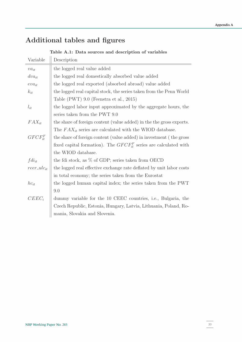
Bureau of Economic Research.
Timmer, M., E. Dietzenbacher, B. Los, R. Stehrer, and G. de Vries
(2015): “An Illustrated User Guide to the World Input-Output Database: the
Case of Global Automotive Production,” Review of International Economics,
23, 575–605.
Wagner, J. (2007): “Exports and Productivity: A Survey of the Evidence from
Firm-level Data,”World Economy, 30, 60–82.
Wang, Z., S.-J. Wei, and K. Zhu (2013): “Quantifying International Pro-
duction Sharing at the Bilateral and Sector Levels,” NBER Working Papers
19677, National Bureau of Economic Research, Inc.
Young, A. (1991): “Learning by Doing and the Dynamic Effects of International
Trade*,”The Quarterly Journal of Economics, 106, 369–405.
31
A Additional tables and figures
Table A.1: Data sources and description of variables
Variable Description
vait the logged real value added
dvait the logged real domestically absorbed value added
evait the logged real exported (absorbed abroad) value added
kit the logged real capital stock, the series taken from the Penn World
Table (PWT) 9.0 (Feenstra et al., 2015)
lit the logged labor input approximated by the aggregate hours, the
series taken from the PWT 9.0
FAXit the share of foreign content (value added) in the the gross exports.
The FAXit series are calculated with the WIOD database.
GFCF Fit the share of foreign content (value added) in investment ( the gross
fixed capital formation). The GFCF Fit series are calculated with
the WIOD database.
fdiit the fdi stock, as % of GDP; series taken from OECD
reer ulcit the logged real effective exchange rate deflated by unit labor costs
in total economy; the series taken from the Eurostat
hcit the logged human capital index; the series taken from the PWT
9.0
CEECi dummy variable for the 10 CEEC countries, i.e., Bulgaria, the
Czech Republic, Estonia, Hungary, Latvia, Lithuania, Poland, Ro-
mania, Slovakia and Slovenia.
32
33NBP Working Paper No. 283
Appendix A
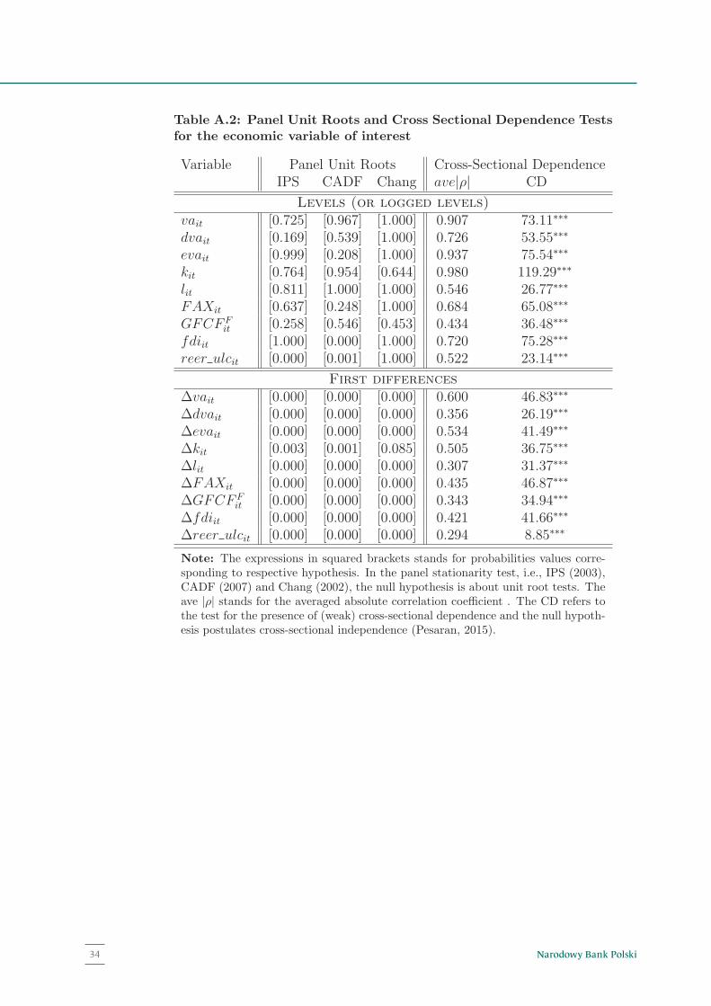
Table A.2: Panel Unit Roots and Cross Sectional Dependence Testsfor the economic variable of interest
Variable Panel Unit Roots Cross-Sectional DependenceIPS CADF Chang ave|ρ| CD
Levels (or logged levels)vait [0.725] [0.967] [1.000] 0.907 73.11∗∗∗
dvait [0.169] [0.539] [1.000] 0.726 53.55∗∗∗
evait [0.999] [0.208] [1.000] 0.937 75.54∗∗∗
kit [0.764] [0.954] [0.644] 0.980 119.29∗∗∗
lit [0.811] [1.000] [1.000] 0.546 26.77∗∗∗
FAXit [0.637] [0.248] [1.000] 0.684 65.08∗∗∗
GFCF Fit [0.258] [0.546] [0.453] 0.434 36.48∗∗∗
fdiit [1.000] [0.000] [1.000] 0.720 75.28∗∗∗
reer ulcit [0.000] [0.001] [1.000] 0.522 23.14∗∗∗
First differencesΔvait [0.000] [0.000] [0.000] 0.600 46.83∗∗∗
Δdvait [0.000] [0.000] [0.000] 0.356 26.19∗∗∗
Δevait [0.000] [0.000] [0.000] 0.534 41.49∗∗∗
Δkit [0.003] [0.001] [0.085] 0.505 36.75∗∗∗
Δlit [0.000] [0.000] [0.000] 0.307 31.37∗∗∗
ΔFAXit [0.000] [0.000] [0.000] 0.435 46.87∗∗∗
ΔGFCF Fit [0.000] [0.000] [0.000] 0.343 34.94∗∗∗
Δfdiit [0.000] [0.000] [0.000] 0.421 41.66∗∗∗
Δreer ulcit [0.000] [0.000] [0.000] 0.294 8.85∗∗∗
Note: The expressions in squared brackets stands for probabilities values corre-sponding to respective hypothesis. In the panel stationarity test, i.e., IPS (2003),CADF (2007) and Chang (2002), the null hypothesis is about unit root tests. Theave |ρ| stands for the averaged absolute correlation coefficient . The CD refers tothe test for the presence of (weak) cross-sectional dependence and the null hypoth-esis postulates cross-sectional independence (Pesaran, 2015).
33Table
A.3:Theestim
atesoflaborand
capitalelasticitiesforexported
valueadded
(FE)
(1)
(2)
(3)
(4)
(5)
(6)
(7)
(8)
(9)
(10
(11)
(12)
Δkit
0.078
-0.500
0.186
-0.524
0.166
-0.581
0.066
-0.429
0.279
-0.770
∗0.233
-0.575
(0.243)
(0.459)
(0.238)
(0.447)
(0.229)
(0.433)
(0.245)
(0.474)
(0.231)
(0.432)
(0.227)
(0.426)
Δl it
0.580∗
∗∗0.574∗
∗∗0.596∗
∗∗0.709∗
∗∗0.532∗
∗∗0.519∗
∗∗0.580∗
∗∗0.531**0.545∗
∗∗0.793∗
∗∗0.548∗
∗∗0.622∗
∗∗
(0.108)
(0.208)
(0.106)
(0.205)
(0.102)
(0.196)
(0.109)
(0.213)
(0.103)
(0.197)
(0.101)
(0.194)
CEEC
i×
Δkit
0.774
0.932∗
∗1.005∗
∗0.669
1.417∗
∗∗1.085**
(0.483)
(0.472)
(0.459)
(0.500)
(0.461)
(0.451)
CEEC
i×
Δl it
0.077
-0.110
0.099
0.172
-0.277
-0.059
(0.227)
(0.224)
(0.213)
(0.238)
(0.218)
(0.213)
ΔFAX
it0.889∗
∗∗0.597∗
∗0.629∗
∗∗0.189
(0.183)
(0.249)
(0.179)
(0.251)
CEEC
i×
ΔFAX
it0.468∗
0.661∗
∗
(0.269)
(0.269)
Δreer
cpi it
-0.401
∗∗∗-0.360
∗∗∗
-0.361
∗∗∗-0.382
∗∗∗
(0.053)
(0.101)
(0.053)
(0.106)
CEEC
i×
Δreer
cpi it
-0.072
-0.007
(0.120)
(0.124)
Δfdi it
0.004
0.004
(0.007)
(0.008)
CEEC
i×
Δfdi it
0.128∗
(0.073)
ΔGFCF
F it0.871∗
∗∗0.711∗
∗∗
(0.119)
(0.159)
CEEC
i×
ΔGFCF
F it0.416∗
∗
(0.209)
μ0.030∗
∗∗0.032∗
∗∗0.030∗
∗∗0.033∗
∗∗0.031∗
∗∗0.033∗
∗∗0.031∗
∗∗0.036∗
∗∗0.024**0.028∗
∗∗0.030∗
∗∗0.034∗
∗∗
(0.011)
(0.011)
(0.010)
(0.010)
(0.010)
(0.010)
(0.011)
(0.011)
(0.010)
(0.010)
(0.010)
(0.010)
Note:thesuperscripts
∗∗∗ ,
∗∗an
d∗denotetherejectionof
nullab
outparam
eters’
insign
ificance
at1%,5%
and10%
significance
level,respectively.The
expressionsin
roundbracketsstan
dsforrobust
stan
darderrors.
34Narodowy Bank Polski34
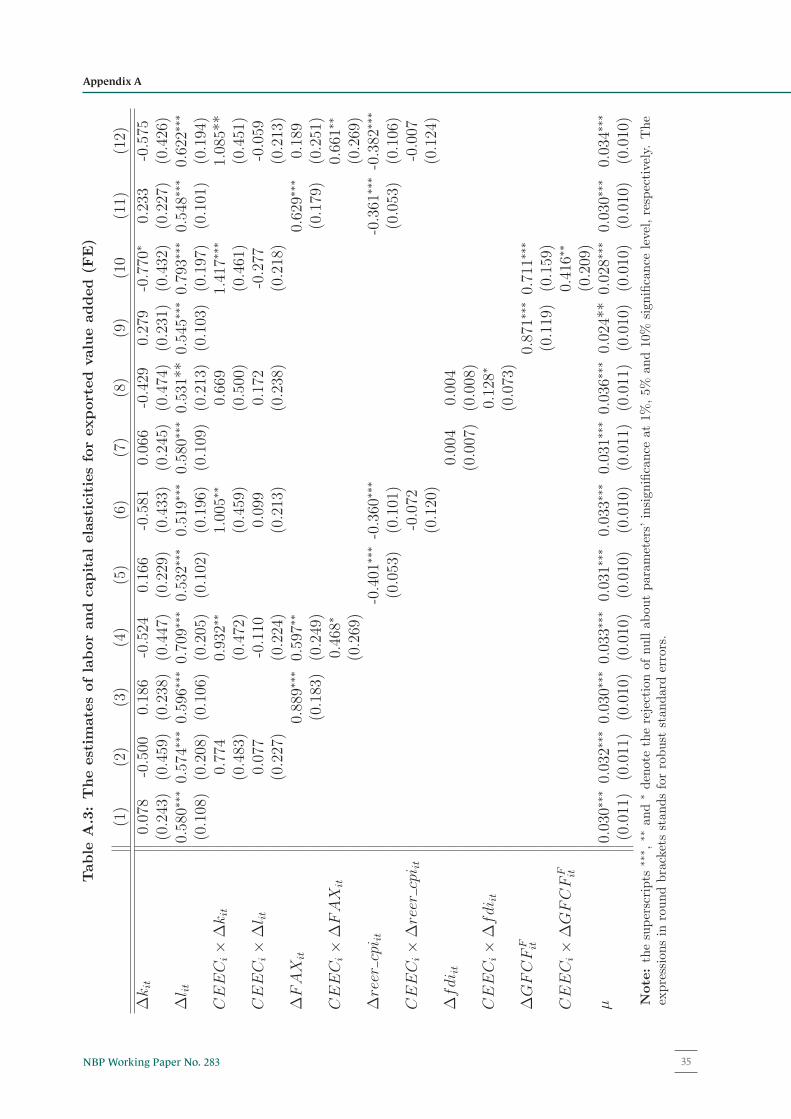
Table A.2: Panel Unit Roots and Cross Sectional Dependence Testsfor the economic variable of interest
Variable Panel Unit Roots Cross-Sectional DependenceIPS CADF Chang ave|ρ| CD
Levels (or logged levels)vait [0.725] [0.967] [1.000] 0.907 73.11∗∗∗
dvait [0.169] [0.539] [1.000] 0.726 53.55∗∗∗
evait [0.999] [0.208] [1.000] 0.937 75.54∗∗∗
kit [0.764] [0.954] [0.644] 0.980 119.29∗∗∗
lit [0.811] [1.000] [1.000] 0.546 26.77∗∗∗
FAXit [0.637] [0.248] [1.000] 0.684 65.08∗∗∗
GFCF Fit [0.258] [0.546] [0.453] 0.434 36.48∗∗∗
fdiit [1.000] [0.000] [1.000] 0.720 75.28∗∗∗
reer ulcit [0.000] [0.001] [1.000] 0.522 23.14∗∗∗
First differencesΔvait [0.000] [0.000] [0.000] 0.600 46.83∗∗∗
Δdvait [0.000] [0.000] [0.000] 0.356 26.19∗∗∗
Δevait [0.000] [0.000] [0.000] 0.534 41.49∗∗∗
Δkit [0.003] [0.001] [0.085] 0.505 36.75∗∗∗
Δlit [0.000] [0.000] [0.000] 0.307 31.37∗∗∗
ΔFAXit [0.000] [0.000] [0.000] 0.435 46.87∗∗∗
ΔGFCF Fit [0.000] [0.000] [0.000] 0.343 34.94∗∗∗
Δfdiit [0.000] [0.000] [0.000] 0.421 41.66∗∗∗
Δreer ulcit [0.000] [0.000] [0.000] 0.294 8.85∗∗∗
Note: The expressions in squared brackets stands for probabilities values corre-sponding to respective hypothesis. In the panel stationarity test, i.e., IPS (2003),CADF (2007) and Chang (2002), the null hypothesis is about unit root tests. Theave |ρ| stands for the averaged absolute correlation coefficient . The CD refers tothe test for the presence of (weak) cross-sectional dependence and the null hypoth-esis postulates cross-sectional independence (Pesaran, 2015).
33
Table
A.3:Theestim
atesoflaborand
capitalelasticitiesforexported
valueadded
(FE)
(1)
(2)
(3)
(4)
(5)
(6)
(7)
(8)
(9)
(10
(11)
(12)
Δkit
0.078
-0.500
0.186
-0.524
0.166
-0.581
0.066
-0.429
0.279
-0.770
∗0.233
-0.575
(0.243)
(0.459)
(0.238)
(0.447)
(0.229)
(0.433)
(0.245)
(0.474)
(0.231)
(0.432)
(0.227)
(0.426)
Δl it
0.580∗
∗∗0.574∗
∗∗0.596∗
∗∗0.709∗
∗∗0.532∗
∗∗0.519∗
∗∗0.580∗
∗∗0.531**0.545∗
∗∗0.793∗
∗∗0.548∗
∗∗0.622∗
∗∗
(0.108)
(0.208)
(0.106)
(0.205)
(0.102)
(0.196)
(0.109)
(0.213)
(0.103)
(0.197)
(0.101)
(0.194)
CEEC
i×
Δkit
0.774
0.932∗
∗1.005∗
∗0.669
1.417∗
∗∗1.085**
(0.483)
(0.472)
(0.459)
(0.500)
(0.461)
(0.451)
CEEC
i×
Δl it
0.077
-0.110
0.099
0.172
-0.277
-0.059
(0.227)
(0.224)
(0.213)
(0.238)
(0.218)
(0.213)
ΔFAX
it0.889∗
∗∗0.597∗
∗0.629∗
∗∗0.189
(0.183)
(0.249)
(0.179)
(0.251)
CEEC
i×
ΔFAX
it0.468∗
0.661∗
∗
(0.269)
(0.269)
Δreer
cpi it
-0.401
∗∗∗-0.360
∗∗∗
-0.361
∗∗∗-0.382
∗∗∗
(0.053)
(0.101)
(0.053)
(0.106)
CEEC
i×
Δreer
cpi it
-0.072
-0.007
(0.120)
(0.124)
Δfdi it
0.004
0.004
(0.007)
(0.008)
CEEC
i×
Δfdi it
0.128∗
(0.073)
ΔGFCF
F it0.871∗
∗∗0.711∗
∗∗
(0.119)
(0.159)
CEEC
i×
ΔGFCF
F it0.416∗
∗
(0.209)
μ0.030∗
∗∗0.032∗
∗∗0.030∗
∗∗0.033∗
∗∗0.031∗
∗∗0.033∗
∗∗0.031∗
∗∗0.036∗
∗∗0.024**0.028∗
∗∗0.030∗
∗∗0.034∗
∗∗
(0.011)
(0.011)
(0.010)
(0.010)
(0.010)
(0.010)
(0.011)
(0.011)
(0.010)
(0.010)
(0.010)
(0.010)
Note:thesuperscripts
∗∗∗ ,
∗∗an
d∗denotetherejectionof
nullab
outparam
eters’
insign
ificance
at1%,5%
and10%
significance
level,respectively.The
expressionsin
roundbracketsstan
dsforrobust
stan
darderrors.
3435NBP Working Paper No. 283
Appendix A
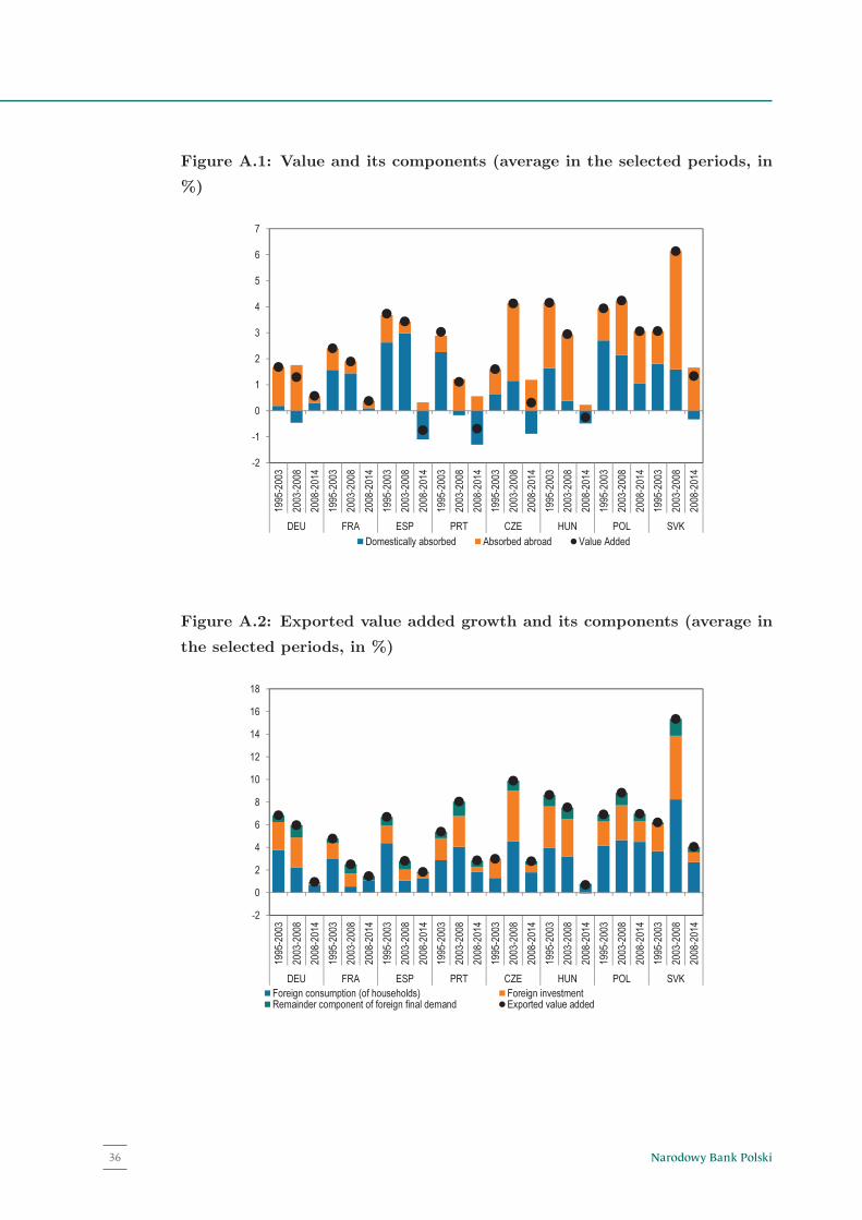
Figure A.1: Value and its components (average in the selected periods, in
%)
-2
-1
0
1
2
3
4
5
6
7
1995-2003
2003-2008
2008-2014
1995-2003
2003-2008
2008-2014
1995-2003
2003-2008
2008-2014
1995-2003
2003-2008
2008-2014
1995-2003
2003-2008
2008-2014
1995-2003
2003-2008
2008-2014
1995-2003
2003-2008
2008-2014
1995-2003
2003-2008
2008-2014
DEU FRA ESP PRT CZE HUN POL SVK
Domestically absorbed Absorbed abroad Value Added
Figure A.2: Exported value added growth and its components (average in
the selected periods, in %)
-2
0
2
4
6
8
10
12
14
16
18
1995-2003
2003-2008
2008-2014
1995-2003
2003-2008
2008-2014
1995-2003
2003-2008
2008-2014
1995-2003
2003-2008
2008-2014
1995-2003
2003-2008
2008-2014
1995-2003
2003-2008
2008-2014
1995-2003
2003-2008
2008-2014
1995-2003
2003-2008
2008-2014
DEU FRA ESP PRT CZE HUN POL SVK
Foreign consumption (of households) Foreign investment
Remainder component of foreign final demand Exported value added
35
Narodowy Bank Polski36
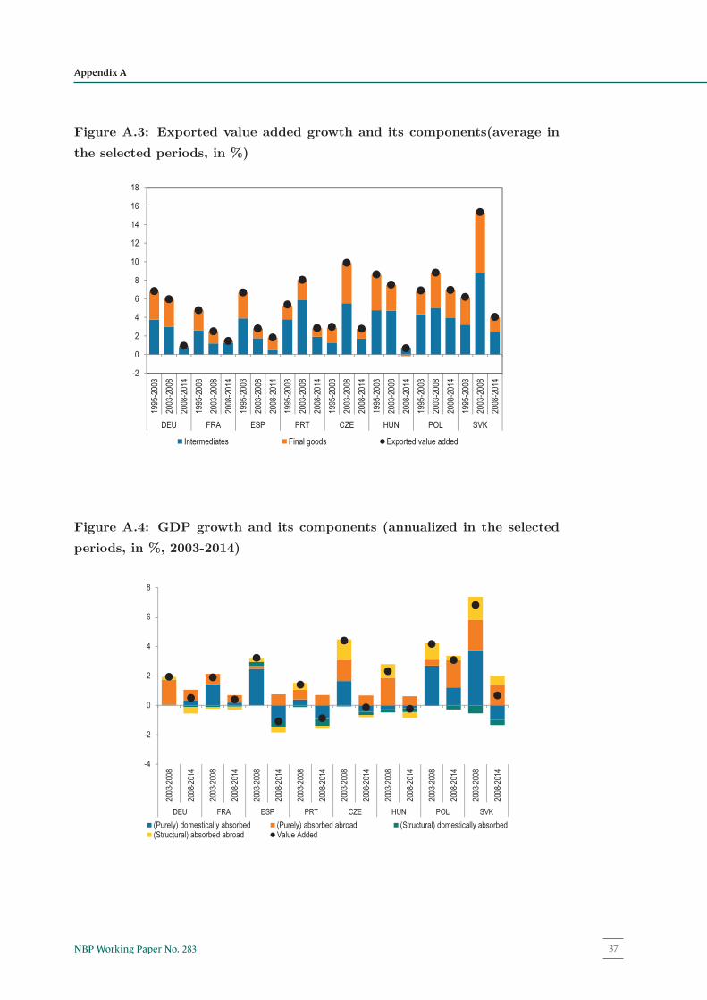
Figure A.1: Value and its components (average in the selected periods, in
%)
-2
-1
0
1
2
3
4
5
6
7
1995-2003
2003-2008
2008-2014
1995-2003
2003-2008
2008-2014
1995-2003
2003-2008
2008-2014
1995-2003
2003-2008
2008-2014
1995-2003
2003-2008
2008-2014
1995-2003
2003-2008
2008-2014
1995-2003
2003-2008
2008-2014
1995-2003
2003-2008
2008-2014
DEU FRA ESP PRT CZE HUN POL SVK
Domestically absorbed Absorbed abroad Value Added
Figure A.2: Exported value added growth and its components (average in
the selected periods, in %)
-2
0
2
4
6
8
10
12
14
16
18
1995-2003
2003-2008
2008-2014
1995-2003
2003-2008
2008-2014
1995-2003
2003-2008
2008-2014
1995-2003
2003-2008
2008-2014
1995-2003
2003-2008
2008-2014
1995-2003
2003-2008
2008-2014
1995-2003
2003-2008
2008-2014
1995-2003
2003-2008
2008-2014
DEU FRA ESP PRT CZE HUN POL SVK
Foreign consumption (of households) Foreign investment
Remainder component of foreign final demand Exported value added
35
Figure A.3: Exported value added growth and its components(average in
the selected periods, in %)
-2
0
2
4
6
8
10
12
14
16
18
1995-2003
2003-2008
2008-2014
1995-2003
2003-2008
2008-2014
1995-2003
2003-2008
2008-2014
1995-2003
2003-2008
2008-2014
1995-2003
2003-2008
2008-2014
1995-2003
2003-2008
2008-2014
1995-2003
2003-2008
2008-2014
1995-2003
2003-2008
2008-2014
DEU FRA ESP PRT CZE HUN POL SVK
Intermediates Final goods Exported value added
Figure A.4: GDP growth and its components (annualized in the selected
periods, in %, 2003-2014)
-4
-2
0
2
4
6
8
2003-2008
2008-2014
2003-2008
2008-2014
2003-2008
2008-2014
2003-2008
2008-2014
2003-2008
2008-2014
2003-2008
2008-2014
2003-2008
2008-2014
2003-2008
2008-2014
DEU FRA ESP PRT CZE HUN POL SVK
(Purely) domestically absorbed (Purely) absorbed abroad (Structural) domestically absorbed
(Structural) absorbed abroad Value Added
36
37NBP Working Paper No. 283
Appendix A
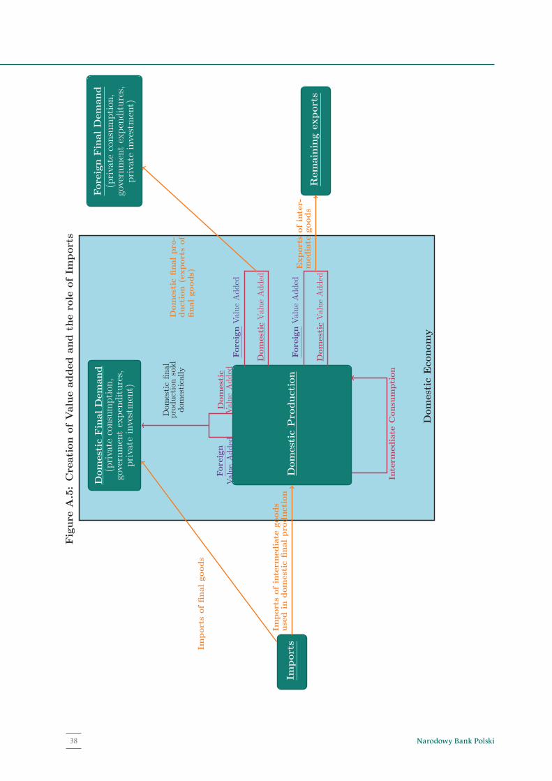
Figure
A.5:Cre
ation
ofValueadded
and
thero
leofIm
ports
Domestic
FinalDemand
(private
consumption
,governmentexpenditures,
private
investment)
ForeignFinalDemand
(private
consumption
,governmentexpenditures,
private
investment)
Domestic
Pro
duction
Remainingexports
Imports
Importsofinterm
ediate
goods
used
indomestic
finalpro
duction
Importsoffinalgoods
Domestic
Eco
nomy
Interm
ediate
Consu
mption
Fore
ign
ValueAdded
Domestic
ValueAdded
Dom
esticfinal
productionsold
dom
estically
Fore
ignValueAdded
Domestic
ValueAdded
Fore
ignValueAdded
Domestic
ValueAdded
Domestic
finalpro
-duction
(exportsof
finalgoods)
Exportsofinter-
mediate
goods
37
Narodowy Bank Polski38
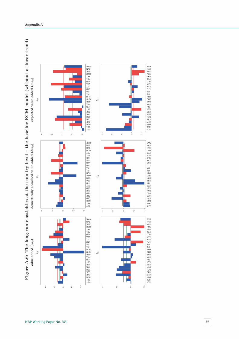
Figure
A.6:Thelong-run
elasticitiesatth
ecountrylevel–th
ebaselineECM
model(w
ithoutalineartrend)
valueadded
(vait)
kit
-1-.50.51
AUTBELBGRCYPCZEDEUDNKESPESTFINFRAGBRGRCHUNIRLITALTULUXLVANLDPOLPRTROUSVKSVNSWE
l it
-.50.51
AUTBELBGRCYPCZEDEUDNKESPESTFINFRAGBRGRCHUNIRLITALTULUXLVANLDPOLPRTROUSVKSVNSWE
domesticallyabso
rbed
valueadded
(dvait)
kit
-1-.50.51
AUTBELBGRCYPCZEDEUDNKESPESTFINFRAGBRGRCHUNIRLITALTULUXLVANLDPOLPRTROUSVKSVNSWE
l it
-1-.50.51
AUTBELBGRCYPCZEDEUDNKESPESTFINFRAGBRGRCHUNIRLITALTULUXLVANLDPOLPRTROUSVKSVNSWE
exported
valueadded
(evait)
kit
0.511.52
AUTBELBGRCYPCZEDEUDNKESPESTFINFRAGBRGRCHUNIRLITALTULUXLVANLDPOLPRTROUSVKSVNSWE
l it
-10123
AUTBELBGRCYPCZEDEUDNKESPESTFINFRAGBRGRCHUNIRLITALTULUXLVANLDPOLPRTROUSVKSVNSWE
38
39NBP Working Paper No. 283
Appendix A
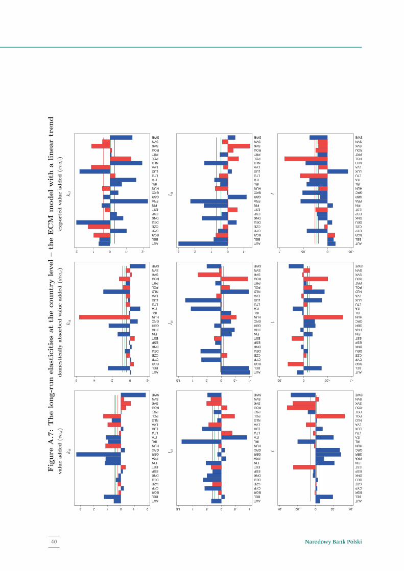
Figure
A.7:Thelong-run
elasticitiesatth
ecountrylevel–th
eECM
modelwith
alineartrend
valueadded
(vait)
kit
-2-10123
AUTBELBGRCYPCZEDEUDNKESPESTFINFRAGBRGRCHUNIRLITALTULUXLVANLDPOLPRTROUSVKSVNSWE
l it
-1-.50.511.5
AUTBELBGRCYPCZEDEUDNKESPESTFINFRAGBRGRCHUNIRLITALTULUXLVANLDPOLPRTROUSVKSVNSWE
t
-.04-.020.02.04
AUTBELBGRCYPCZEDEUDNKESPESTFINFRAGBRGRCHUNIRLITALTULUXLVANLDPOLPRTROUSVKSVNSWE
domesticallyabso
rbed
valueadded
(dvait)
kit
-20246
AUTBELBGRCYPCZEDEUDNKESPESTFINFRAGBRGRCHUNIRLITALTULUXLVANLDPOLPRTROUSVKSVNSWE
l it
-1-.50.511.5
AUTBELBGRCYPCZEDEUDNKESPESTFINFRAGBRGRCHUNIRLITALTULUXLVANLDPOLPRTROUSVKSVNSWE
t
-.1-.050.05
AUTBELBGRCYPCZEDEUDNKESPESTFINFRAGBRGRCHUNIRLITALTULUXLVANLDPOLPRTROUSVKSVNSWE
exported
valueadded
(evait)
kit
-2-1012
AUTBELBGRCYPCZEDEUDNKESPESTFINFRAGBRGRCHUNIRLITALTULUXLVANLDPOLPRTROUSVKSVNSWE
l it
-10123
AUTBELBGRCYPCZEDEUDNKESPESTFINFRAGBRGRCHUNIRLITALTULUXLVANLDPOLPRTROUSVKSVNSWE
t
-.050.05.1
AUTBELBGRCYPCZEDEUDNKESPESTFINFRAGBRGRCHUNIRLITALTULUXLVANLDPOLPRTROUSVKSVNSWE
39Narodowy Bank Polski40
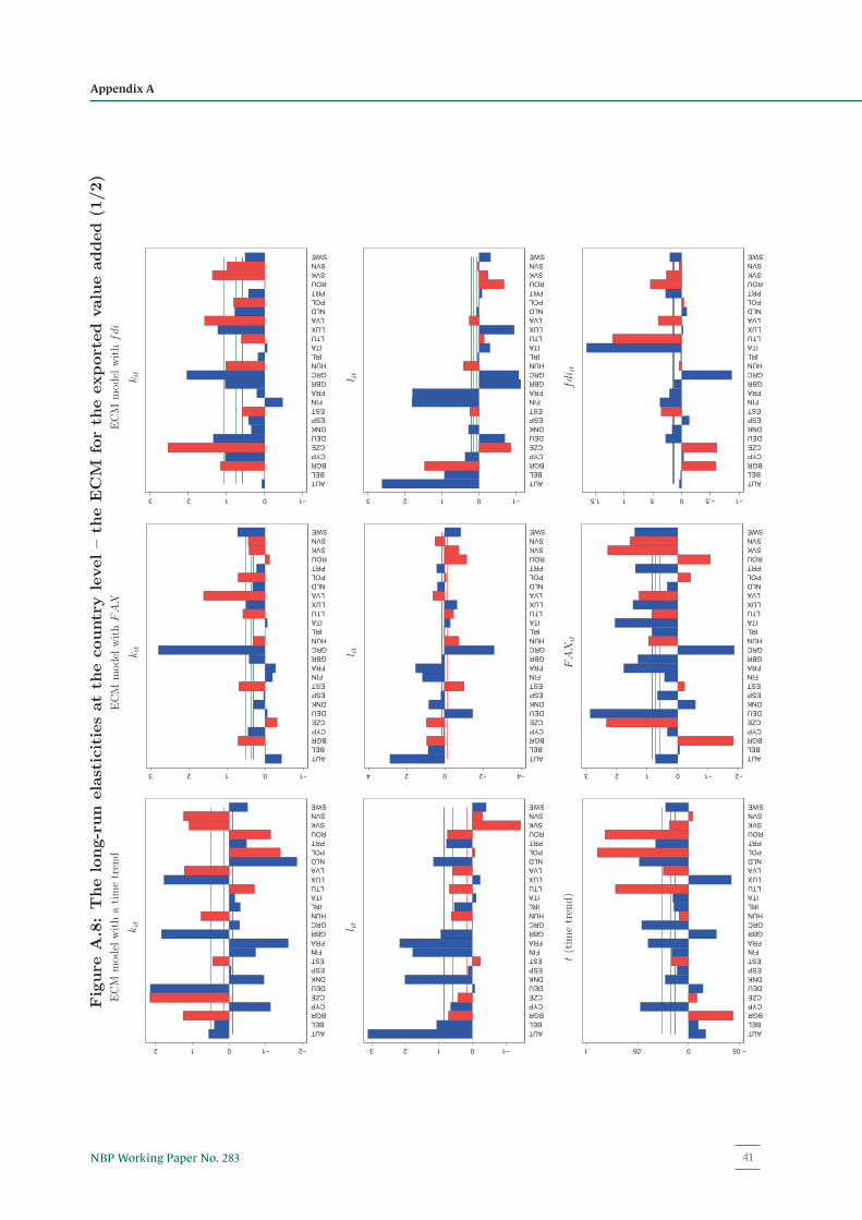
Figure
A.8:Thelong-run
elasticitiesatth
ecountrylevel–th
eECM
forth
eexported
valueadded
(1/2)
ECM
model
withatimetrend
kit
−2−1012
AUTBELBGRCYPCZEDEUDNKESPESTFINFRAGBRGRCHUNIRLITALTULUXLVANLDPOLPRTROUSVKSVNSWE
l it
−10123
AUTBELBGRCYPCZEDEUDNKESPESTFINFRAGBRGRCHUNIRLITALTULUXLVANLDPOLPRTROUSVKSVNSWE
t(tim
etrend)
−.050.05.1
AUTBELBGRCYPCZEDEUDNKESPESTFINFRAGBRGRCHUNIRLITALTULUXLVANLDPOLPRTROUSVKSVNSWE
ECM
model
withFAX
kit
−10123
AUTBELBGRCYPCZEDEUDNKESPESTFINFRAGBRGRCHUNIRLITALTULUXLVANLDPOLPRTROUSVKSVNSWE
l it
−4−2024
AUTBELBGRCYPCZEDEUDNKESPESTFINFRAGBRGRCHUNIRLITALTULUXLVANLDPOLPRTROUSVKSVNSWE
FAX
it
−2−10123
AUTBELBGRCYPCZEDEUDNKESPESTFINFRAGBRGRCHUNIRLITALTULUXLVANLDPOLPRTROUSVKSVNSWE
ECM
model
withfdi
kit
−10123
AUTBELBGRCYPCZEDEUDNKESPESTFINFRAGBRGRCHUNIRLITALTULUXLVANLDPOLPRTROUSVKSVNSWE
l it
−10123
AUTBELBGRCYPCZEDEUDNKESPESTFINFRAGBRGRCHUNIRLITALTULUXLVANLDPOLPRTROUSVKSVNSWE
fdi it
−1−.50.511.5
AUTBELBGRCYPCZEDEUDNKESPESTFINFRAGBRGRCHUNIRLITALTULUXLVANLDPOLPRTROUSVKSVNSWE
40
41NBP Working Paper No. 283
Appendix A
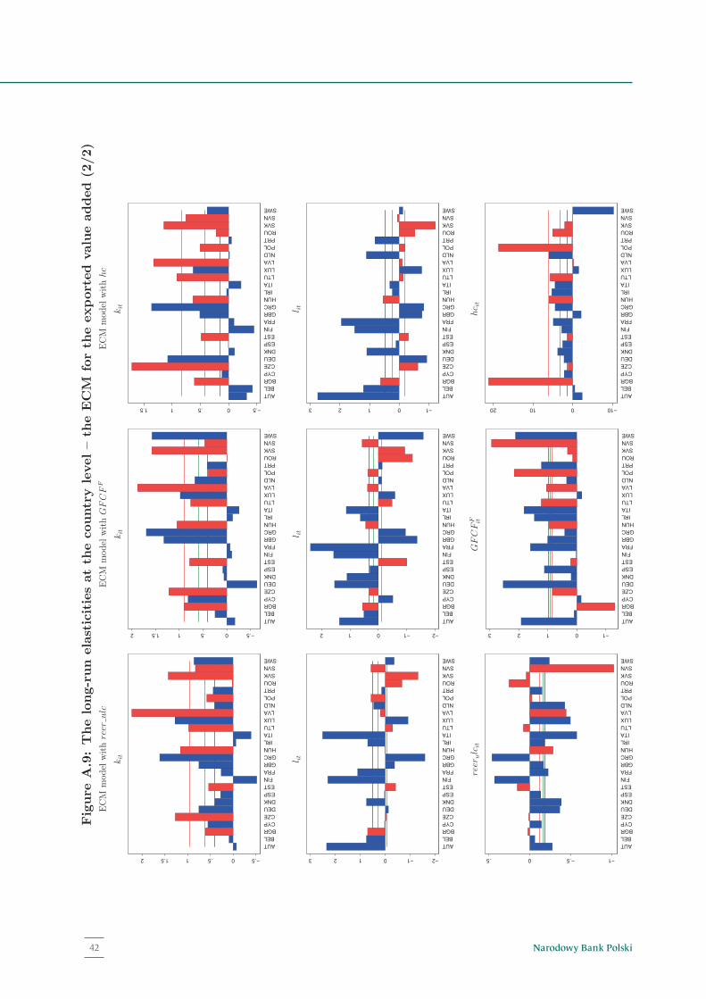
Figure
A.9:Thelong-run
elasticitiesatth
ecountrylevel–th
eECM
forth
eexported
valueadded
(2/2)
ECM
model
withreer
ulc
kit
−.50.511.52
AUTBELBGRCYPCZEDEUDNKESPESTFINFRAGBRGRCHUNIRLITALTULUXLVANLDPOLPRTROUSVKSVNSWE
l it
−2−10123
AUTBELBGRCYPCZEDEUDNKESPESTFINFRAGBRGRCHUNIRLITALTULUXLVANLDPOLPRTROUSVKSVNSWE
reer
ulc
it
−1−.50.5
AUTBELBGRCYPCZEDEUDNKESPESTFINFRAGBRGRCHUNIRLITALTULUXLVANLDPOLPRTROUSVKSVNSWE
ECM
model
withGFCF
F
kit
−.50.511.52
AUTBELBGRCYPCZEDEUDNKESPESTFINFRAGBRGRCHUNIRLITALTULUXLVANLDPOLPRTROUSVKSVNSWE
l it
−2−1012
AUTBELBGRCYPCZEDEUDNKESPESTFINFRAGBRGRCHUNIRLITALTULUXLVANLDPOLPRTROUSVKSVNSWE
GFCF
F it
−10123
AUTBELBGRCYPCZEDEUDNKESPESTFINFRAGBRGRCHUNIRLITALTULUXLVANLDPOLPRTROUSVKSVNSWE
ECM
model
withhc
kit
−.50.511.5
AUTBELBGRCYPCZEDEUDNKESPESTFINFRAGBRGRCHUNIRLITALTULUXLVANLDPOLPRTROUSVKSVNSWE
l it
−10123
AUTBELBGRCYPCZEDEUDNKESPESTFINFRAGBRGRCHUNIRLITALTULUXLVANLDPOLPRTROUSVKSVNSWE
hc it
−1001020
AUTBELBGRCYPCZEDEUDNKESPESTFINFRAGBRGRCHUNIRLITALTULUXLVANLDPOLPRTROUSVKSVNSWE
41
Narodowy Bank Polski42

www.nbp.pl


