Page 1
URBAN HOUSING AFFORDABILITY IN KENYA
A Case Study of the Mortgage Housing Sector in Nairobi
Kieti Raphael Mutisya
BA (Land Economics), M.A, MISK, R.V
A Thesis Submitted in Fulfillment of the Requirements for the Degree of Doctor of
Philosophy, Department of Real Estate and Construction Management, School of the Built
Environment, University of Nairobi, Kenya.
August, 2015
Page 2
ii
DECLARATION
I hereby declare that this thesis is my original work and has not been presented for a degree in
any other University
……………………………………………….
Raphael Mutisya Kieti
DECLARATION OF THE SUPERVISORS
This thesis has been submitted for examination with our approval as University Supervisors
............................. …………….. ………………
Dr. M. A. Swazuri Prof. S. Masu Dr. J. Murigu
Page 3
iii
ACKNOWLEDGEMENTS
Iam grateful to many people who contributed immensely towards the completion of this
research thesis. Iam particularly indebted to my supervisors Dr. Muhammad Swazuri,
Professor Sylvester Masu and Dr. Jennifer Murigu for their critique, scrutiny and useful
guidance. Their unrelenting understanding, support and patience helped me continue with the
research work despite my other assignments at the Ministry of Lands. Iam grateful to
Professor Paul Syagga with whom I discussed my first research proposal at the time when I
was conceiving the research problem. I acknowledge with thanks his kind help and
encouragement. Iam also grateful to Dr. Margaret Gachuru for her guidance and
encouragement. Thanks also to Catherine Kariuki, Nicky Nzioki, Dr. Winnie Mwangi, Dr.
Mary Kimani, Dr. Konyimbih, Professor Robert Rukwaro and all the other staff members in
the Department of Real Estate and Construction Management at the University of Nairobi.
I appreciate with thanks the kind help extended by my research assistants, Seth Gikunda and
Royford Kinyua who assisted in data collection and analysis at various stages during the
preparation of the research thesis. Iam grateful to Martin Kimeu of the Ministry of Housing
for his help in data analysis and compilation of the final research report. My gratitude further
goes to all who in one way or another provided research materials. Special mention is due for
the help received from Peter Kimeu and Jacob Wambua both of Housing Finance Limited
who facilitated data availability and accessibility. Without their help this study would have
taken a much longer period to complete.
I cherish the friendship, inspiration and support of my colleagues in Valuation Section at the
Ministry of Lands, Housing and Urban Development, who have over the years persistently
encouraged and inspired me to complete my research study and aim higher. Iam particularly
grateful to the Government Chief Valuer, Mr. Anthony Itui who agreed to my request for a
transfer to Nairobi after a two year stay in Kajiado District. This enabled me to focus on my
research work and made possible regular consultation with my supervisors and access to
library and internet materials available at the Ministry headquarters in Nairobi. To all my
other colleaques- Nora Nyakora, Monica Obong’o, Eva Njoroge, Ruth Kiviu, Rose Karago,
Bernard Nzau, George Ruhara I say thank you very much.
Page 4
iv
In the end, words will always be inadequate in thanking God for his blessings and for making
everything possible.
Raphael M. Kieti
University of Nairobi, Kenya
Page 5
v
DEDICATION
I dedicate this work to the victims of slums fire disasters all over the world and especially the
victims of the SINAI FIRE DISASTER that occurred in Nairobi, Kenya (September 12,
2011), whose lives would have been saved if decent housing was accessible and affordable to
all.
Page 6
vi
ABSTRACT
Over 70 % of urban households in Kenya experience severe housing affordability challenges.
Affordability problems are manifested in the high levels of homelessness, poor human
settlement conditions, high price of housing relative to the incomes of households, mortgage
delinquencies, defaults and foreclosures. This study investigated factors affecting housing
affordability in Kenya. Previous studies on housing in Kenya have been descriptive in nature
and little or no emphasis has been made on empirical studies on factors affecting affordability
especially with regard to contribution of the factors to housing affordability. The result has
been a lack of knowledge on which factors are critical in explaining the affordability
problems of urban households in Kenya. The objectives of this research work were therefore
to: identify significant factors that affect housing affordability, determine the influence of the
significant factors and rank them with respect to contribution to housing affordability and,
suggest policies necessary to address the urban housing affordability problem in Kenya.
The research focused on affordability in the home-ownership mortgage housing sector in
Nairobi. The methodology was based on a questionnaire survey to households with mortgage
loans from Housing Finance Institutions and Banks. A total sample size of 390 households
was targeted for the study. However, 353 households responded to the survey yielding a
response rate of 90.5%. Information relating to social-economic characteristics of the
households, loan and property data as well as macroeconomic data was analyzed in order to
address the objectives of the study. The analyses were done using qualitative and quantitative
approaches with the aid of the Statistical Package for Social Sciences (SPSS) software. Three
statistical procedures, namely; descriptive statistics, correlation analysis and regression
analysis were performed on the data with the aim of identifying factors which are significant
predictors of housing affordability.
The research found that there is a significant linear relationship between housing affordability
and the factors: Interest on loan, Number of dependants (outside the nuclear family), Number
of family members with income, Construction cost, Size of the household, Loan-to-value
(LTV) ratio, Land value, Real gross domestic product (GDP) per capita, Job position/status of
the individual paying the mortgage, Type of mortgage instrument, Loan term, Loss of regular
employment income and the rate of inflation. The results indicated that the interest charged
on mortgage loan has the greatest influence on the affordability of the households. The
interest on loan which reflects the mortgage interest rate charged by the banks influence
Page 7
vii
affordability because it determines the borrower’s monthly mortgage repayment amounts.
The results showed that an increase in the amount of interest charged on the loan increases
the monthly loan repayment placing a higher repayment burden on the households thus
affecting their affordability.
Applying Multiple Regression Analysis (MRA) to determine the contribution of the
significant factors and, therefore, rank them with respect to contribution to affordability, the
results showed that eight (8) factors namely; Interest on loan, Number of dependants (outside
the nuclear family), Loan-to- value (LTV) ratio, type of mortgage instrument, Number of
family members with income, Loan term, real GDP per capita and size of the household,
have a significant contribution to affordability and are therefore the most critical factors that
influence affordability in the home ownership (mortgage) housing sector in Kenya.
The regression model comprising of the eight critical factors has a correlation coefficient (R)
of 0.833 and a coefficient of determination (R2) of 0.693. The model has a significant F-
value of 97.127, indicating that the eight factors are significant predictors of housing
affordability. Among the eight factors, interest on loan is the most important factor
accounting for 52.8% of the variance in affordability, while the size of household is the least
important factor.
From the literature review and the results of the analyses performed in this study, it was
concluded that housing affordability is influenced by clusters of factors related to the
households’ social economic characteristics, loan characteristics, property attributes and
macro-economic factors. The households social economic characteristics among others
include; the Loss of regular employment income, Number of dependants, Number of family
members with income and Size of the household. The loan factors include the Interest
charged on loan, Loan-to-value (LTV) ratio, Loan term and the Type of mortgage instrument.
The property attributes are the Cost of construction, Land value, Developers profit and
Property transfer costs. The macro economic factors include the Rate of inflation, Real gross
domestic (GDP) per capita and Unemployment rate.
The results of the analyses showed that the social economic factors affect affordability
because they influence households’ income. The loan factors influence affordability because
they affect the price of housing and the monthly mortgage repayments of the households.The
property factors affect the price of housing and therefore the monthly loan repayments. The
macro economic factors affect both the income of households and housing price as well as
Page 8
viii
mortgage interest rates charged by the banks and financial institutions. Policy measures have
been proposed to reduce or stabilize mortgage interest rates, reduce the price of housing, and
improve household’s income so as to enhance access to housing and improve affordability
among urban households in Kenya.
The research thesis is organized into six chapters. Chapter one covers the general background
to the study in the form of introduction, problem statement, study objectives and hypothesis
as well the significance and limitations of the study. At the end of the chapter, the
organization of the study is presented. Chapter two provides a general over view of the urban
housing problem with reference to developing countries. The purpose of the review is to
develop a frame work and lay a solid foundation necessary to contextualize the urban housing
affordability problem generally and in particular factors affecting affordability in Kenya.
Chapter three provides the theoretical and conceptual framework of the study. In particular,
the theories that explain the urban housing affordability problem in developing countries are
identified and explained. Review of theories in research studies is important because they
offer a theoretical basis for undertaking the research study. Theories explain the phenomenon
that is being studied and offers tentative theoretical answers or solutions to the problem that
is being investigated. The last section of the chapter reviews literature on the factors affecting
affordability and formulates a conceptual model of affordability and its determining factors.
Chapter four defines the research design and methodology adopted to address the research
questions and objectives of the study. The chapter begins with a brief description of the case
study area, Nairobi, its location in Kenya, population dynamics and the housing situation that
necessitates the need for policy interventions to address the affordability challenges of
households in the City and Kenya in general. The chapter then discusses the research design
adopted for the study by highlighting the sources and types of data used, the procedures
employed in deriving the research variables and a description of the relevant variables and
data used in the study. Chapter five identifies the factors that affect housing affordability in
the home ownership mortgage housing sector and ranks them with respect to contribution to
affordability. Chapter six provides a summary and discussion of the main research findings,
the conclusions drawn from the research findings as well as contribution to knowledge,
policy recommendations and suggested areas of further research.
Page 9
ix
TABLE OF CONTENTS
Page
TITLE…………………………………………………………………………………… i
DECLARATION……………………………………………………………………….. ii
ACKNOWLEDGEMENTS……………………………………………………………. iii
DEDICATION……………………………………………………………………………..v
ABSTRACT …………………………………………………………………………… vi
TABLE OF CONTENTS……………………………………………………………..… ix
LIST OF TABLES …………………………………………………………………….. xii
LIST OF FIGURES ………………………………………………………………..... xiii
LIST OF ABBREVIATIONS………………………………………………...……… xiii
CHAPTER 1: INTRODUCTION AND BACKGROUND TO THE STUDY..….…...1
1.0 Introduction ....................................................................................................................1
1.1 Problem Statement…………………………………………………………………… 4
1.2 Study Hypothesis…………………………………………………………………….10
1.3 Research Objectives .....................................................................................................11
1.4 Research Questions………………………………………………………………….. 11
1.5 Scope of the Study .......................................................................................................11
1.6 Significance of the Study ............................................................................................13
1.7 Limitations of the Study ……………………………………………………………. 13
1.8 Organization of the Study............................................................................................14
1.9 Summary……………………………………………………………………….…......15
CHAPTER 2: AN OVERVIEW OF THE URBAN HOUSING PROBLEM…....… 17
2.0 Introduction ..................................................................................................................17
2.1 Housing Deficits ..........................................................................................................18
2.2 Housing Conditions .....................................................................................................22
2.3 Housing Finance...........................................................................................................25
2. 3.1 Forms of Housing Finance…………………………………………………………27
2.3.1.1 Debt Finance...........................................................................................................27
2.3.1.2. Equity Finance.......................................................................................................27
Page 10
x
2.3.2 Sources of Housing Finance for Lenders..................................................................28
2.3.3. Housing Finance Markets in Developing Countries................................................31
2.4. Housing Affordability.................................................................................................38
2.4.1. Affordability Measures............................................................................................40
2.4.1.1. The Ratio Measures..............................................................................................41
2.4.1.2. Residual Measures................................................................................................43
2.4.1.3. Other Measures…………………………………………………….………....…44
2.4.2. Housing Affordability Problems in Developing Countries.....................................45
2.5 Summary .....................................................................................................................49
CHAPTER 3. HOUSING AFFORDABILITY- TOWARDS A THEORETICAL AND
CONCEPTUAL FRAMEWORK……………………………………51
3.0 Introduction ..................................................................................................................51
3.1 Theories of Housing Affordability...............................................................................52
3.1.1 Public Interest Economic Regulation Theory (PIERT) ............................................53
3.1.2 The Theory of Distributive Justice ...........................................................................56
3.2 Special Characteristics of Housing ..............................................................................59
3.3 State Intervention vs. Free- Market Debate in Housing Affordability ........................62
3.4. Factors Affecting Housing Affordability...................................................................64
3.4.1. Demand-Side Factors...............................................................................................68
3.4.2. Supply-Side Factors.................................................................................................71
3.5. A Conceptual Model of Factors Affecting Affordability..........................................72
3.6 Summary……………………………………………………………………………75
CHAPTER 4: RESEARCH DESIGN AND METHODOLOGY.…………....……..76
4.0 Introduction ................................................................................................................76
4.1 Over view of Nairobi City..……………………………...…………………………..76
4.2. Research Design..........................................................................................................78
4.2.1. Population, Sample Size and Sampling Techniques................................................80
4.2.2 Data Collection…………………………………………………………..….….….86
4.3 Variable Identification, Description and Measurement………………….……….….87
4.3.1. The Dependent Variable..........................................................................................88
4.3.2. Independent Variables.............................................................................................89
4.4 Method Used to Rate the Factors that Affect Housing Affordability……………..101
Page 11
xi
4.5 Testing the Hypothesis using the Population Mean Score…………………….……103
4.6 Testing the Hypothesis using the Critical Z- value ………………………………...103
4.7. Data Analysis.............................................................................................................105
4.7.1. The Multiple Regression Analysis (MRA) Technique...........................................106
4.7. 2. Performing Multiple Regression using SPSS........................................................109
4.8. Summary…………………………………………………………………………..111
CHAPTER 5: FACTORS THAT AFFECT AFFORDABILITY IN THE MORTGAGE
HOUSING SECTOR IN KENYA...……………………………….112
5.0 Introduction ...............................................................................................................112
5.1 Factors that Affect Affordability in the
Mortgage Housing Sector in Kenya ..........................................................................112
5.2 Significant Factors Affecting Housing Affordability ................................................117
5.3. Significant Factor Contribution to Housing Affordability.......................................130
5.3.1. Descriptive Statistics..............................................................................................133
5.3.2. Correlation Analysis...............................................................................................138
5.3.3. Regression Analysis...............................................................................................146
5.3.4 Selecting the Appropriate Regression Model.........................................................160
5.3.5 Hypothesis Testing ……………………………………………………………….162
5.4. Summary....................................................................................................................162
CHAPTER 6: SUMMARY, CONCLUSIONS, POLICY RECOMMENDATIONS AND
AREAS OF FURTHER RESEARCH....………………………….…165
6.0. Introduction...............................................................................................................165
6.1. Summary and Discussion of Results……………………………………………….165
6.2. Conclusions................................................................................................................178
6.2.1. Contribution to Knowledge………………………………………………………180
6.3. Policy Recommendations…………………………………………………………..181
6.4 Areas of Further Research...………………………………………………………...188
BIBLIOGRAPHY.……………………………………………………………..…..….189
Page 12
xii
APPENDICES……………………………………………………………………..….. 201
Appendix A: Questionnaire to Households in Nairobi………………………………... 201
Appendix B: Households Social-Economic Characteristics………………………..….209
Appendix C: Households Mortgage Data………………………………………………243
Appendix D: Households Property Data………………………………………………..268
Appendix E: Macro- Economic Indicators 2000-2013………………………………….288
LIST OF TABLES
Table 1.1 Residential Mortgages Market Perfomance 2011&2012..………….………..7
Table 1.2 Average Wage Earnings per Employee, 2009-2013 (kshs. Per annum)……..8
Table 2.1 Housing needs and Housing Backlogs in selected African Countries…….. 19
Table 2.2 Distribution of the world’s urban slum dwellers, 2001…………………….23
Table 2.3 Mortgages as a % of GDP in Selected African Countries………….………32
Table 2.4 Number of Mortgage Accounts and Mortgages Outstanding in 2012……..37
Table 2.5 Relationship of Income to House price in selected Countries in Africa….…46
Table 4.1 Total Number of Mortgage Loans, Sample Size and Responses from
Households for each year (2000-2012)…………………………………..….82
Table 4.2 Summary of the Variables………………………………………..……….100
Table 4.3 Critical Value of Z…………………………………………………..…….104
Table 5.0 Rating of the Variables by the Respondents ………………………….…...118
Table 5.1 Mean Rating of the Factors Affecting Housing Affordability………....…120
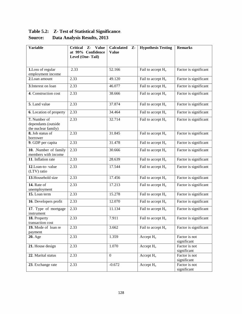
Table 5.2 Z- Test of Statistical Significance……………………………………...…128
Table 5.3 Significant Factors Affecting Housing Affordability…………………….129
Table 5.4 Descriptive Statistics of the Dependent Variable, Housing Affordability..135
Table 5.5 Descriptive Statistics of Independent Variables…………………………..137
Table 5.6 Correlation Results (Dependent and Independent Variables)……….……141
Table 5.7 First Regression Results (Model Summary)…………………………….…149
Table 5.8 Analysis of Variance (ANOVA)………………………………………….149
Table 5.9 First Regression Results (Model Coefficients)…………………………….150
Table 5.10 Final Regression Results (Model Summary)……………………………….154
Page 13
xiii
Table 5.11 Analysis of Variance (ANOVA)…………………………………………..154
Table 5.12 Final Regression Results (Model Coefficients)……………………………155
Table 5.13 STEPWISE Regression Results (Model Coefficients)…………………….159
Table 5.14 STEPWISE Regression Results (Model Summary)…………………….…160
LIST OF FIGURES
Figure 3.0 Factors Affecting Housing Affordability……………………………………74
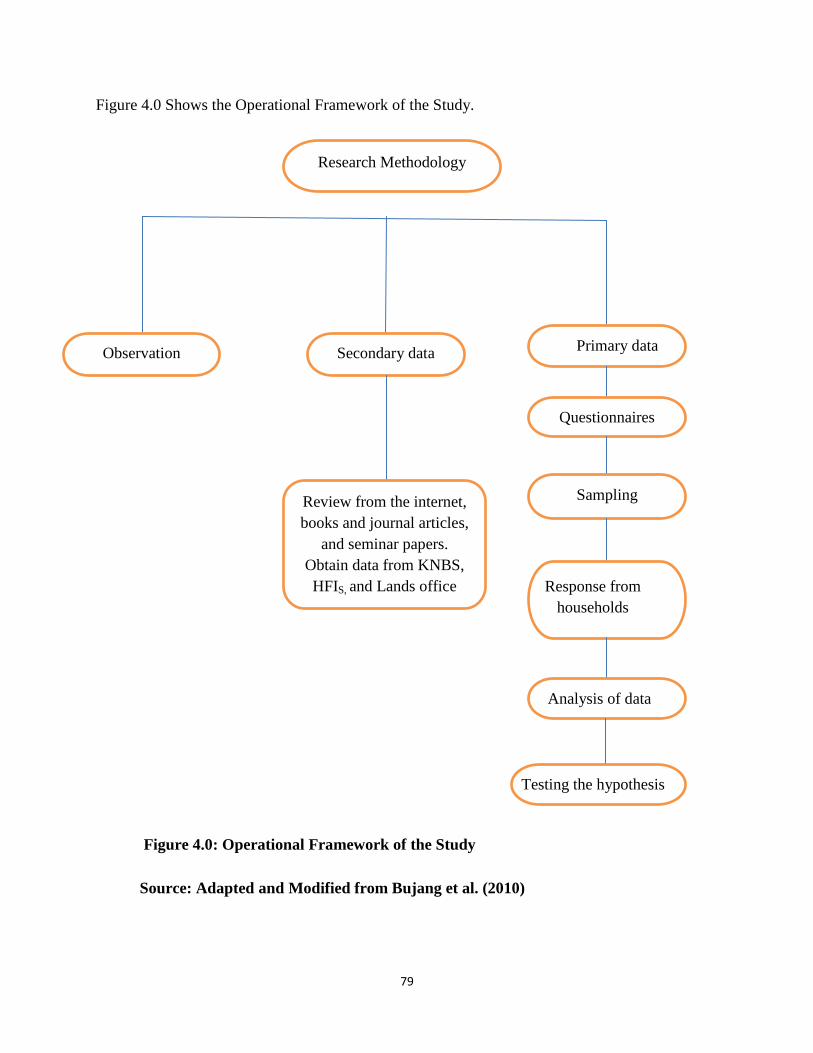
Figure 4.0 Showing the Operational Framework of the Study………………………….79
Figure 5.0 Histogram and Normal Curve for the Dependent Variable, Housing
Affordability……………………………………………………………..…135
LIST OF GRAPHS, CHARTS AND MAPS
Graph 1.0 Value and Number of Non-Performing (NPLs) Mortgages 2011-2014 ………6
Graph 2.0 Relationship of Income to House price in selected Countries of Africa……..47
Graph 3.0 Housing Market in Equilibrium State …………………………………….….65
Graph 3.0a Housing Market with a Shift in the Supply Curve ……………………….….66
Graph 3.0b Housing Market with a Shift in Demand Curve …………………………….67
Map 4.0 Showing Boundary of the Present Day Nairobi indicating the Main
Administrative Divisions and Subdivisions………………………………….77
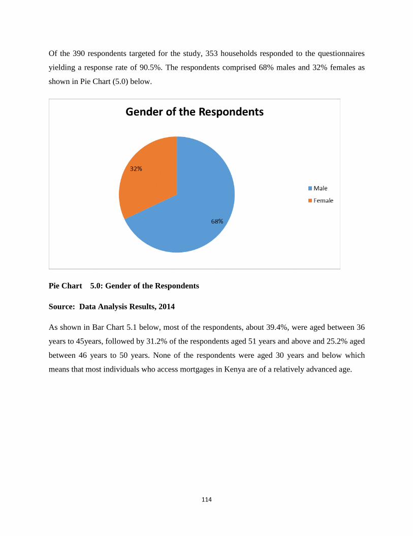
Pie Chart 5.0 Gender of the Respondents …………………………………….………….114
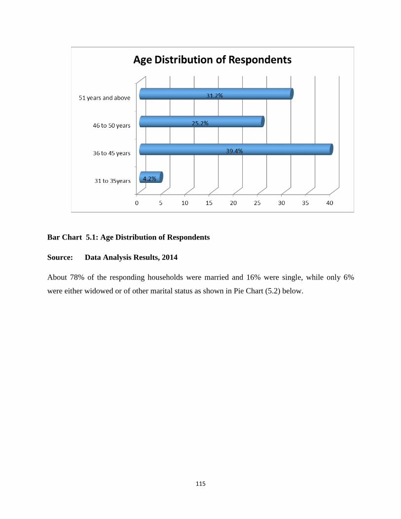
Bar Chart 5.1 Age Distribution of the Respondents …………………………….………. 115
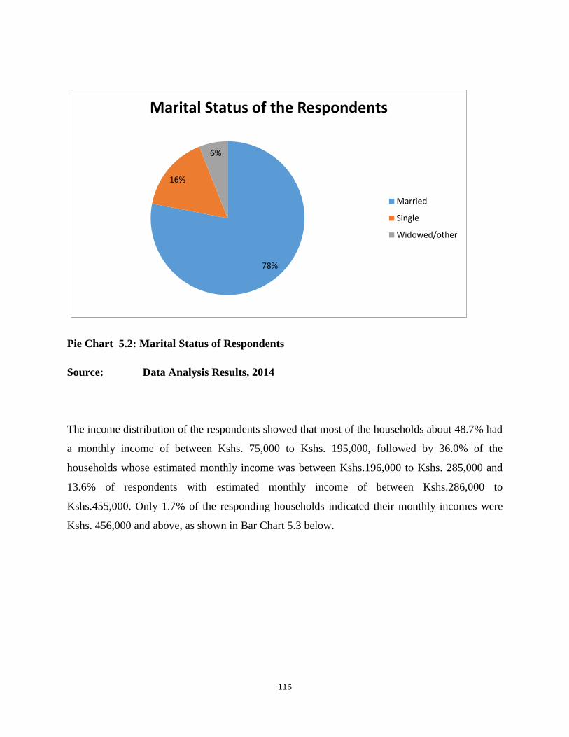
Pie Chart 5.2 Marital Status of the Respondents ……………………………….…….…..116
Bar Chart 5.3 Income Distribution of the Respondents ……………………….……..……117
LIST OF ABBREVIATIONS
AFDB African Development Bank
AHURI Australian Housing and Urban Research Institute
ARM Adjustable Rate Mortgages
ANHS Australian National Housing Strategy
BAI Banco Africano De Investimento
BBK Barclays Bank of Kenya
Page 14
xiv
CAHF Centre for Affordable Housing Finance
CBK Central Bank of Kenya
CGT Capital Gains Tax
CMA Capital Markets Authority
CRBs Credit Reference Bureaus
CRI Collateral Replacement Indemnity
CFC CFC Stanbic Bank
CPI Consumer Price Index
COHRE Centre on Housing Rights and Evictions
DBL Development Bank Limited
EMCA Environmental Management and Coordination Act
EA Environmental Audit
EIA Environmental Impact Assessment
EFInA Enhancing Financial Innovation and Access
FXBs Forex Bureaus
FRM Fixed Rate Mortgages
GDP Gross Domestic Product
GNI Gross National Income
GCR Greater Cairo Region
HFIs Housing Finance Institutions
HFCK Housing Finance Company of Kenya/ Housing Finance
HIDTF Housing Infrastructure Development Trust Fund
IMF International Monetary Fund
IRA Insurance Regulatory Authority
JCHS Joint Centre for Housing Studies
KCB Kenya Commercial Bank
KIPPRA Kenya Institute of Public Policy Research and Analysis
KSHS Kenya Shillings
KNBS Kenya National Bureau of Statistics
LRP Land Readjustment Program
LTP Land Taxation Policy
LTV Loan -to- Value Ratio
LPTs Listed Property Trusts
MBS Mortgage Backed Securities
Page 15
xv
MRA Multiple Regression Analysis
MFC Mortgage Finance Company
MFW4A Making Finance Work for Africa
MLF Mortgage Liquidity Facility
NCEO City of Nairobi Environment Outlook
NGOs Non Governmental Organizations
NHFC National Housing Finance Corporation of South Africa
NPLs Non Performing Loans
NSE Nairobi Securities Exchange
NSW New South Wales
PMIs Primary Mortgage Institutions
PIERT Public Interest Economic Regulation Theory
REITs Real Estate Investment Trusts
SPSS Statistical Package for Social Sciences
SACCOs Savings and Credit Cooperative Societies
TMRC Tanzania Mortgage Refinance Company
UN- HABITAT United Nations Human Settlement Programme
UNCHS United Nations Centre for Human Settlement
US United States of America
US DOLLAR United States of America Dollar
VIF Variance Inflation Factor
Page 16
1
CHAPTER 1
INTRODUCTION AND BACKGROUND TO THE STUDY
1.0 Introduction
Housing is regarded as a system made up of shelter and the supporting basic infrastructure
required by man. It is a basic human need in every society and is considered a fundamental right
of every individual (Akinwunmi, 2009). The right to housing is embedded in various
international instruments including the United Nations Human Rights Declaration of 1948, the
International Covenant on Economic, Social and Cultural Rights of 1966, the Istanbul
Declaration and Habitat Agenda of 1996 and the Declaration on Cities and other Human
Settlements of 2001(Republic of Kenya, 2004). The right to housing is further embedded in the
Constitution of Kenya 2010. Article 43 (1b) of the Constitution provides that every person has
the right to accessible and adequate housing, and to reasonable standards of sanitation. Nabutola
(2004) has equated shelter to food, which is a human need, so much so that those who cannot
afford it still need it.
Since the early times, man has made relentless efforts to obtain housing. The struggle for this
basic need has increased progressively as the human race has advanced in numbers and cultural
diversity. Housing has economic, social and political roles and is an indicator of development
and welfare in a country (Chirchir, 2006). On the economic front, investment in housing
contributes towards reducing poverty, generating employment, raising incomes, improving
health and increasing productivity of the labour force. Housing plays a major role in serving as
an asset (Alhashin and Dwyer, 2004). For a typical house-owner, the house is a major asset in his
portfolio and for many households, the purchase of a house represents the largest (and often
only) lifelong investment and a store of wealth. Socially, housing has substantial benefits
including the welfare effects of shelter from the elements, sanitation facilities and access to
health and education services (Chirchir, 2006). Habitable housing contributes to the health,
efficiency, social behavior and general welfare of the populace (Nubi, 2008). Improved health
and education and better access to income earning opportunities can lead to higher productivity
and earnings for families. Housing plays the role of promoting privacy, dignity, safety and status
among people. Politically, proper housing reduces political unrest emanating from shelter
Page 17
2
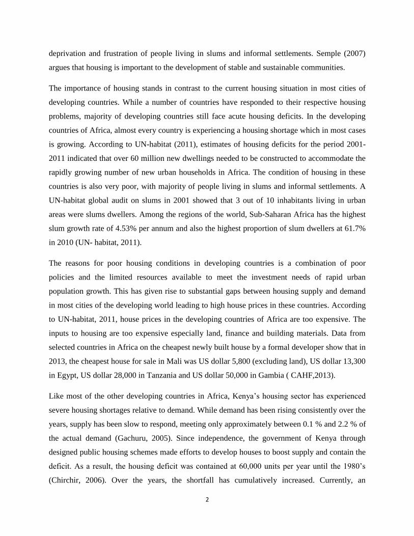
deprivation and frustration of people living in slums and informal settlements. Semple (2007)
argues that housing is important to the development of stable and sustainable communities.
The importance of housing stands in contrast to the current housing situation in most cities of
developing countries. While a number of countries have responded to their respective housing
problems, majority of developing countries still face acute housing deficits. In the developing
countries of Africa, almost every country is experiencing a housing shortage which in most cases
is growing. According to UN-habitat (2011), estimates of housing deficits for the period 2001-
2011 indicated that over 60 million new dwellings needed to be constructed to accommodate the
rapidly growing number of new urban households in Africa. The condition of housing in these
countries is also very poor, with majority of people living in slums and informal settlements. A
UN-habitat global audit on slums in 2001 showed that 3 out of 10 inhabitants living in urban
areas were slums dwellers. Among the regions of the world, Sub-Saharan Africa has the highest
slum growth rate of 4.53% per annum and also the highest proportion of slum dwellers at 61.7%
in 2010 (UN- habitat, 2011).
The reasons for poor housing conditions in developing countries is a combination of poor
policies and the limited resources available to meet the investment needs of rapid urban
population growth. This has given rise to substantial gaps between housing supply and demand
in most cities of the developing world leading to high house prices in these countries. According
to UN-habitat, 2011, house prices in the developing countries of Africa are too expensive. The
inputs to housing are too expensive especially land, finance and building materials. Data from
selected countries in Africa on the cheapest newly built house by a formal developer show that in
2013, the cheapest house for sale in Mali was US dollar 5,800 (excluding land), US dollar 13,300
in Egypt, US dollar 28,000 in Tanzania and US dollar 50,000 in Gambia ( CAHF,2013).
Like most of the other developing countries in Africa, Kenya’s housing sector has experienced
severe housing shortages relative to demand. While demand has been rising consistently over the
years, supply has been slow to respond, meeting only approximately between 0.1 % and 2.2 % of
the actual demand (Gachuru, 2005). Since independence, the government of Kenya through
designed public housing schemes made efforts to develop houses to boost supply and contain the
deficit. As a result, the housing deficit was contained at 60,000 units per year until the 1980’s
(Chirchir, 2006). Over the years, the shortfall has cumulatively increased. Currently, an
Page 18
3
estimated 750,000 and 1,500,000 households in urban and rural areas respectively are in need of
housing (Republic of Kenya, 2004). The estimated current urban housing needs are 150,000 units
per year while the production rate of new houses is estimated at only 20,000- 30,000 units
annually, giving a housing shortage of over 120,000 units per year.
According to Chirchir (2006), the key factors among many that have contributed to this
unprecedented housing shortage include the government’s reduced budgetary allocation on
public housing and infrastructure development, high rural-urban migration rate that has stretched
housing demand in urban areas, high cost of land and building materials and the limited and high
cost of housing finance. The effect of these factors as well as the rapid increase in the urban
population of towns and cities in Kenya have further widened the supply/demand gap inevitably
leading to the high prices and rents being charged on housing. This has given rise to affordability
challenges among urban households in Kenya. Problems of affordability have been exacerbated
by the low income levels of households. Poverty statistics in Kenya show high number of people
living below the designated poverty line (Economic Survey, 2014). In Nairobi, 22% of the
population live in poverty (CAHF, 2012). According to the Africa Housing Finance Year Book
2012, by the Centre for Affordable Housing Finance in Africa (CAHF), only about 11% of
Kenyans earn enough to support a mortgage. This means that most households cannot afford an
average mortgage necessary to buy an entry-level house. Affordability is currently the main
urban housing challenge affecting the urban population in Kenya. While efforts have been
undertaken to tackle this challenge, the affordability problem has persisted and is more acute
among low and middle income groups in society. In order to tackle this problem, there is need to
investigate the significant factors that affect housing affordability in Kenya. Further, there is
need to determine the contribution of the factors to housing affordability. Knowledge of the
significant factors and their contribution to affordability is essential for the development and
design of appropriate policies to tackle the serious challenge of housing affordability in Kenya.
Page 19
4
1.1 Problem Statement
During the last three decades, Kenya has been experiencing very rapid urbanization resulting
from natural population growth and large-scale rural-urban migration driven by rapid social
economic changes and development. This phenomenon of urbanization has brought with it
enormous challenges manifested in the acute shortage of housing resulting to overcrowding, high
house prices, substandard human settlement conditions such as slums and squatter settlements,
inadequate infrastructure, community facilities and services (Obudho and Aduwo, 1998;
Kusienya, 2004). The acute housing shortage in Kenya has given rise to serious affordability
challenges as demand for housing continue to outstrip supply. The affordability problems are
manifested in the high levels of homelessness, poor human settlement conditions, high price of
housing relative to the incomes of households, mortgage delinquencies, defaults and
foreclosures.
House prices in Kenya’s urban centres have increased tremendously over the last decade.
Property values have increased by over 3 times since year 2000. The average value of a property
grew from Kshs. 7.1 million in 2000 to Kshs. 22.3 million in 2012 (HFCK, 2012). The Hass
Consult property index shows property price rise of 1.3% in 2012 and 1.4% in 2011. The price
for both detached and semi-detached houses rose by 1.8%, while apartment prices increased by
2.3% in 2013(Hass Consult Report, 2013). According to the Africa Housing Finance Year book
2012 and 2013 by the Centre for Affordable Housing Finance in Africa (CAHF), the cheapest
newly built house by a formal developer in Kenya costs between US dollar 13,000 and US dollar
18,000 and would require a monthly income of US dollar 677 with a 10% deposit on a 20 year
mortgage at 19% interest rate. Given a statutory minimum wage of US dollar 162 in Kenya, it
would take on average the equivalent of between 7 to 9 salary years for a household on the
minimum wage to complete paying the mortgage for the cheapest house. This is based on the
assumption that the household shall spend all its earnings on housing which is unrealistic.
According to the 9th
Demographia International Housing Affordability Survey 2013, households
should not spend more than the equivalent of 3 salary years to complete paying for their
mortgages.
Page 20
5
There are many factors that contribute to the high prices of houses in Kenya, among them, the
cost of land and infrastructure, cost of labour and building materials and the high cost of finance
due to the high interest rates charged by Banks and Financial Institutions. The rates of mortgage
interest in Kenya have been high over the last decade. In the year 2000, for example, interest
rates on mortgages were high at 19% and remained at almost the same level until the year 2002.
The rates of mortgage interest averaged 13% from the year 2003 to 2007. In the year 2011,
interest on mortgages averaged 20%. In the year 2012, interest rates charged by banks in Kenya
were on average 18% and ranged from 11% to 25%, and in 2013, the average interest on
mortgages was 16.89% ranging between 15.5% and 19% (CBK Annual Reports, 2012 and
2013).
The high mortgage interest rate regime that has prevailed in the country over the past years has
impacted negatively on the performance of the mortgage market in Kenya. Consequently, as a
result of the high interest rates, only a tiny proportion of the urban population in Kenya can
afford a mortgage at market interest rate. The Hass Consult Limited estimates that only 50% of
people living in urban areas can service a kshs. 700,000 mortgage, only 4% are able to take up a
kshs. 3.9 million mortgage and only 1% can afford a kshs.5.9 million home loan at the current
interest rates (Hass Consult Ltd, 2013). Given an average mortgage loan size of kshs. 6.4 million
in Kenya, it means that mortgage affordability is limited to a very small proportion of the urban
population.
Affordability problems in the mortgage housing sector in Kenya are manifested by delinquencies
and defaults in loan servicing. According to the Central Bank of Kenya (CBK) mortgage market
survey reports of 2011 and 2012, the value of non- performing mortgage loans (NPLs) increased
from Kshs 3.6 billion in 2011 to Kshs. 6.9billion in 2012, representing an increase of
Kshs.3.3billion, or over 90% growth of non-performing mortgages (CBK Annual Reports, 2011
and 2012). As indicated in Graph 1.0 and Table 1.1, the number of non-performing mortgage
accounts over the same period increased from 764 to 969 accounts, which is a growth of 27% of
non-performing mortgage accounts. The value of non- performing mortgage loans increased to
Kshs. 8.5 billion in 2013 and Kshs. 10.8 billion in 2014, with the number of non-performing
mortgage accounts increasing from 1,280 to 1,474 accounts over the same period (CBK Annual
Reports, 2013 and 2014). The increase in the value and number of non-performing mortgages is
Page 21
6
an indication of affordability challenges experienced by households in the mortgage housing
sector in Kenya.
Value of NPLs Mortgages (Kshs. billions)
No. of NPLs Mortgage Accounts
Graph 1.0 Value and Number of Non-Performing (NPLs) Mortgages 2011- 2014
Source: Author’s Construct with data from CBK Annual Reports of 2011- 2014
2011 2012 2013 2014
Value of NPLs
Mortgages
(Kshs. Billions)
No. of NPLs
Mortgage
Accounts
10.8
8.5
6.9
3.6
1474
1280
969
764
Page 22
7
Table 1.1 Residential Mortgages Market Performance 2011&2012
Source: CBK Annual Reports, 2011 and 2012
Year 2011 2012
Financial Institution Value of
Mortgages
Outstanding
(Ksh. Bns)
Value of
NPLs
Mortgages
(Ksh. Bns)
No. of
Mortgage
Accounts
No. of NPLs
Mortgage
Accounts
Value of
Mortgage
Outstanding
(Ksh. Bns)
Value of
NPLs
Mortgages
(Ksh. Bns)
No. of
Mortgage
Accounts
No. of
NPLs
Mortgage
Accounts
Housing Finance Ltd 25.8 1.6 4,932 310 30.3 2.3 5,235 396
Kenya Commercial
Bank
18.1 1.0 4,073 204 31.5 2.2 5,091 282
CFC Stanbic Bank 8.8 0.83 1,210 9 9.5 0.19 1,340 24
Standard Chartered
Bank
7.8 0.12 1,251 32 9.7 0.16 1,480 30
Barclays Bank Ltd 4.4 0.22 939 14 4.3 0.19 1,021 6
Co-operative Bank Ltd 2.2 0.42 289 1 6.6 0.31 398 33
National Bank Ltd 3.1 0.81 154 18 4.1 0.57 221 15
Consolidated Bank 2.8 0.69 302 4 3.8 0.29 566 28
Equity Bank Ltd 3.4 0.24 682 6 3.7 0.35 702 10
Others 14.2 0.57 2,197 166 18.6 0.74 3,123 145
TOTAL 90.4 3.6 16,029 764 122.2 6.9 19,177 969
Page 23
8
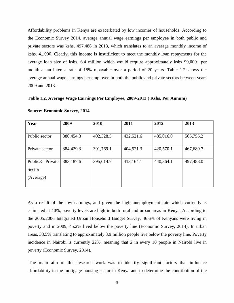
Affordability problems in Kenya are exacerbated by low incomes of households. According to
the Economic Survey 2014, average annual wage earnings per employee in both public and
private sectors was kshs. 497,488 in 2013, which translates to an average monthly income of
kshs. 41,000. Clearly, this income is insufficient to meet the monthly loan repayments for the
average loan size of kshs. 6.4 million which would require approximately kshs 99,000 per
month at an interest rate of 18% repayable over a period of 20 years. Table 1.2 shows the
average annual wage earnings per employee in both the public and private sectors between years
2009 and 2013.
Table 1.2. Average Wage Earnings Per Employee, 2009-2013 ( Kshs. Per Annum)
Source: Economic Survey, 2014
Year 2009 2010 2011 2012 2013
Public sector 380,454.3 402,328.5 432,521.6 485,016.0 565,755.2
Private sector 384,429.3 391,769.1 404,521.3 420,570.1 467,689.7
Public& Private
Sector
(Average)
383,187.6 395,014.7 413,164.1 440,364.1 497,488.0
As a result of the low earnings, and given the high unemployment rate which currently is
estimated at 40%, poverty levels are high in both rural and urban areas in Kenya. According to
the 2005/2006 Integrated Urban Household Budget Survey, 46.6% of Kenyans were living in
poverty and in 2009, 45.2% lived below the poverty line (Economic Survey, 2014). In urban
areas, 33.5% translating to approximately 3.9 million people live below the poverty line. Poverty
incidence in Nairobi is currently 22%, meaning that 2 in every 10 people in Nairobi live in
poverty (Economic Survey, 2014).
The main aim of this research work was to identify significant factors that influence
affordability in the mortgage housing sector in Kenya and to determine the contribution of the
Page 24
9
factors to affordability. While there exist a lot of literature on housing in Kenya, unfortunately,
there is no empirical research on housing affordability and especially on the factors affecting
affordability. There is, therefore, a lack of knowledge on which factors are critical in explaining
the affordability problems of urban households in the mortgage housing sector in Kenya.
Previous studies on housing in Kenya have been descriptive in nature and have focused on the
supply of low cost housing, slums and informal settlements, housing finance and sustainable
housing delivery.
A report by Syagga, Mitullah and Karirah (1999 cited by Warah, 2001), for instance, focused on
slums and informal settlements. Several publications by the United Nations Centre for Human
Settlement (UNCHS) have also extensively examined the urban slum challenge in Kenya.
Nabutola (2004) highlighted the constraints to affordable housing provision. Gachuru (2005)
analyzed the impact of financial de-regulation on mortgage loan performance in Kenya. Chirchir
(2006) examined the potential role of retirement benefits in promoting home- ownership, while
Kiriko (2013) offered a critical analysis of urban housing deficits in Kenya. Clearly, housing
affordability studies have not been given attention in the academic housing literature in Kenya.
However, within the international housing literature, there have been some empirical studies on
factors affecting affordability. Bujang et al (2010) analyzed the relationship between
demographic factors and housing affordability in Johor Bahru in Malaysia and found that
affordability is influenced by four factors related to households’ social economic characteristics,
that is, marital status, level of education, monthly income and number of income earners in a
household. In the study by Mostafa et al (2005) on the relationship between housing affordability
and economic development in Hong Kong, three macro economic factors, that is, gross domestic
product, inflation rate and income were found to have a significant relationship with affordability
in Hong Kong.
The study by Bujang et al (2010) and that of Mostafa et al (2005), however, did not identify the
most critical factor neither did they rank the factors with respect to contribution to affordability.
The subject study bridges that gap by contributing to the empirical analysis of factors affecting
affordability through an objective identification and measurement of the contribution of the
significant factors to mortgage affordability in Kenya.
Page 25
10
Further, while the studies by Bujang et al (2010) and Mostafa et al (2005) are important in
understanding the causes of affordability problems, there is need to identify more social
economic and macro economic factors that influence mortgage affordability. Also, in an effort to
extend the studies and to fully understand the causes of affordability problems, it is important to
investigate other factors that are critical in explaining the affordability problems of households
especially within developing countries like Kenya. Examining the causes of affordability
problems from the point of view of only the social economic and macro economic factors fails to
capture the multi- dimensional nature of affordability. Property attributes like the size and value
of land, cost of construction, developers profit and property transfer costs are important factors in
house price determination and, therefore, have the potential to influence affordability. The
impact of these property related factors on affordability has, however, not been analyzed. The
impact of loan factors like the loan repayment period, loan -to- value ratio and type of mortgage
instrument on mortgage affordability has also not been studied.
In order to fully address the pressing affordability challenges in the mortgage housing sector in
Kenya, this study proposes that the causes of affordability problems should be examined from
the point of view of households’ social economic characteristics, property attributes, loan
characteristics and the macro economic factors. A rigorous analysis of these factors especially
with regard to their contribution to affordability will enrich housing research and give policy on
affordability in Kenya some kind of direction and focus.
1.2. Study Hypothesis
Null Hypothesis (HO): “The interest charged on a mortgage is not the most
important factor that affects housing affordability in Kenya.”
Alternative Hypothesis (HA): “The interest charged on a mortgage is the most important
factor that affects housing affordability in Kenya.”
Page 26
11
1.3. Research Objectives
The specific objectives of the research work are:
i). To identify significant factors that affect affordability in the mortgage housing sector in
Kenya
ii). To determine the influence of the significant factors and rank them with respect to
contribution to housing affordability
iii).To develop a model to guide policy on affordability in the mortgage housing sector in Kenya.
1.4. Research Questions
The study is guided by three fundamental research questions:
i). Which significant factors explain affordability problems of urban households in the mortgage
housing sector in Kenya?
ii). What is the contribution of the factors to housing affordability?
iii).What policy measures are necessary to address the affordability problems of households
in the mortgage housing sector in Kenya?
1.5. Scope and Area of Study
The study focused on urban housing sector and, therefore, considered affordability problems of
urban households. The study was limited to the urban housing sector because urban housing
problems in Kenya are more severe than rural housing problems both in their intensity and
complexity. The main housing problems of rural areas revolve around housing quality issues in
terms of sanitation and infrastructure of existing housing and not affordability. Housing
affordability problems are of less importance in rural areas than in urban areas. In Kenya, urban
areas have higher population growth rates and higher population densities. Urban areas also have
higher costs and values of land and property and higher levels of income and employment
disparity. Consequently, overcrowding, high house prices, slums and informal settlements are
common features of the Kenyan urban land scape. Thus the study focused on the urban sector
because it has more severe housing problems.
Page 27
12
In terms of geographical scope, the study covered Nairobi and considered affordability in the
home-ownership mortgage housing sector. Home-ownership housing sector was considered
because it is the preferred tenure choice by majority of urban households because of the security
and stability it offers as opposed to renting. Mortgage housing was selected for the study because
it offers immediate access to decent and adequate housing as opposed to incremental building.
Mortgage housing is the dominant mode of home acquisition in Nairobi with majority of
households (over 30%) acquiring homes through mortgage financing (Republic of Kenya, 2005,
2009). There is thus the need to find solutions to affordability problems in the mortgage housing
sector in order to promote home-ownership in Kenya.
The study covered households in the four zones/ locations of Nairobi covering residential estates
located in the South of Nairobi which included estates in Langata, South B and South C estates
and also estates off Mombasa Road. The study also included residential estates in the East of
Nairobi covering the estates in Buruburu, Donholm, Savannah, Greenfields and Baraka estate in
Embakasi, among others. The study further included the West of Nairobi including households in
Westlands, Parklands, Ngong Road, Kilimani, Kileleshwa and Lavington, among others. Lastly,
the study covered the North of Nairobi including Rosslyn Estate, Nyari, Runda, Muthaiga,
Thome and Garden estate, among others.
Nairobi is chosen because it is the largest and fastest growing city in Kenya. Nairobi is an
important city in the national economy contributing about 47.5% of the total Gross Domestic
Product (Economic Survey, 2014). Information in Nairobi is accessible and is fairly current and
well documented. Households in Nairobi have a major housing affordability problem with over
60 % of the population living in slums and squatter settlements (Cohre, 2008). Compared to
other towns in Kenya, the population of Nairobi currently estimated at over 3 million people is
high and the number of households estimated at 985,016 households means a higher demand for
housing, hence the high prices and rents charged on housing in Nairobi. Incomes are low and
poverty levels are high with over 22% of households in Nairobi living below the poverty line
(Economic survey, 2014). The dependency ratio, defined as the proportion of the population in
Nairobi that is dependent is currently high at 52.7% and this ratio is much higher among the poor
at 71.3%. Home-ownership rate in Nairobi is quite low at 7.6% compared to 87.9% of
households who rent their accommodation. The low incidence of home-ownership is attributed to
Page 28
13
the high cost of housing and the low incomes of households which explain the pressing
affordability challenges of households in Nairobi. Understanding the factors affecting
affordability in Nairobi, therefore, serves as a useful guide towards understanding and
appreciating the general urban housing affordability problem in Kenya.
1.6. Significance of the Study
The analyses and findings from this research are of interest to researchers, academicians and
policy makers. Researchers and housing experts are keen to understand the affordability
determinants which are relevant and significant in the Kenyan mortgage housing sector.
Knowledge of the significant affordability determinants would guide policy makers in housing
policy formulation to achieve immediate and sustained housing affordability which is necessary
towards the realization of Kenya Vision 2030. The Vision 2030 strategy envisions a Nation that
is adequately and decently housed in a sustainable environment. The main goal of Vision 2030
with regard to housing is to increase production of housing and to achieve better development
and access to affordable housing among all the households in Kenya. The findings emanating
from this research would help economic planners and policy makers to design appropriate and
more focused policies targeting the factors which have been found in this study to be more
critical in explaining affordability problems of households in the mortgage housing sector in
Kenya. The findings would also help in providing information necessary to guide general
economic policy formulation and intervention programmes affecting the housing sector of the
economy. Further, given the current dearth of empirical studies on mortgage housing
affordability, this study constitutes an important pioneering work and contributes towards filling
the existing literature gap in this area of housing research in Kenya as well as other countries.
1.7 Limitations of the Study
The key limitations encountered in the course of this study were data related, mainly, inherent in
the information on which the study relied upon. The study sought to analyse affordability of
households with mortgages from Housing Finance Institutions (HFIs) and Banks in Kenya.
Information from these institutions was difficult to get and despite numerous efforts, only one
Housing Finance Institution, that is, the Housing Finance Limited agreed to release its data.
Whereas relying on mortgage data from only one Financial Institution has the potential to affect
Page 29
14
the outcome of the study, The Housing Finance Limited accounts for over 25 % of all mortgages
in Kenya and upto 40% of all the Mortgages in Nairobi. The information obtained from Housing
Finance Limited was thus taken as representative of the mortgage market in Kenya. Further, data
on macro-economic factors affecting affordability were obtained from secondary sources, for
example, Annual Economic Survey Reports and yearly Statistical Abstracts from the Kenya
National Bureau of Statistics (KNBS). Current information on some macro economic data from
these secondary documents was not available thus posing a limitation to the study.
1.8. Organization of the Study
The study is organized into six chapters. Chapter one covers the general introduction of the study
in the form of introduction, problem statement, study objectives and hypothesis as well as the
significance and limitations of the study. At the end of the chapter, the organization of the study
is presented. Chapter two provides a general overview of the urban housing problem with
reference to developing countries. The purpose of the review is to develop a frame work and lay
a solid foundation necessary to contextualize the urban housing affordability problem generally
and in particular factors affecting affordability in Kenya.
Chapter three provides the theoretical and conceptual framework of the study. In particular, the
theories that explain the urban housing affordability problem in developing countries are
identified and explained.Theory plays an essential role in research as it guides the development
of research questions, selection of methodologies, and interpretation of results. Most importantly,
the utilization of theory is necessary for the advancement of knowledge. Further, review of
theories in research studies is important because they offer a theoretical basis for undertaking the
research study. Theories explain the phenomenon that is being studied and offers tentative
theoretical answers or solutions to the problem that is being investigated. The last section of the
chapter reviews literature on the factors affecting affordability and formulates a conceptual
model of affordability and its determining factors.
Chapter four defines the research design and methodology adopted to address the research
questions and objectives of the study. The chapter begins with a brief description of the case
study area, Nairobi, its location in Kenya, population dynamics and the housing situation that
necessitates the need for policy interventions to address the affordability challenges of
Page 30
15
households in the City and Kenya in general. The chapter then discusses the research design
adopted for the study by highlighting the sources and types of data used, the procedures
employed in deriving the research variables and a description of the relevant variables and data
used in the study. Chapter five identifies the factors that affect housing affordability in the home
ownership mortgage housing sector and ranks them with respect to contribution to affordability.
Chapter six provides a summary and discussion of the main research findings, the conclusions
drawn from the research findings as well as contribution to knowledge, policy recommendations
and suggested areas of further research.
1.9 Summary
This chapter has presented the general introduction and broad justification of the study. The
affordability problem of the urban housing challenge in Kenya has also been explained.
Generally, the high cost of housing, the low incomes of households and the proliferation of
slums and squatter settlements in the urban areas of Kenya are the most vivid manifestation of
affordability problems. House prices in Kenya’s urban centres are high relative to the incomes of
the households. House prices have increased tremendously over the last decade. Property values
have increased by over 3 times since year 2000. Many factors have contributed to the high price
of housing in Kenya, among them the cost of land and infrastructure, cost of labour and building
materials and the high cost of finance due to the high interest rate charged by banks and financial
institutions.
The rates of mortgage interest in Kenya have been high over the last decade. In the year 2000 for
example, interest rates on mortgages were high at 19% and remained at almost the same level
until the year 2002. The rates of mortgage interest averaged 13% from the year 2003 to 2007. In
the year 2011, interest on mortgages averaged 20%. In the year 2012, interest rates charged by
banks in Kenya were on average 18% and ranged from 11% to 25%, and in 2013, the average
interest on mortgages was 16.89% ranging between 15.5% and 19%. The high mortgage interest
rate regime that has prevailed in the Country over the past years has impacted negatively on the
performance of the mortgage market in Kenya with non- performing loans increasing from Kshs.
3.6 billion in 2011 to kshs. 6.9 billion in 2012. As a result of the high interest rates, only a tiny
proportion of the urban population in Kenya can afford a mortgage at market interest rate.
Page 31
16
Household incomes on the other hand have been low and have not grown to match the rapid
increase in house prices. Average monthly income based on wage earnings in Kenya is kshs.
41,000/= and is insufficient to meet the monthly loan repayments of kshs. 99,000 for the average
mortgage size at current mortgage interest rates.
The factors that affect affordability of urban households in the home ownership (mortgage)
sector in Kenya can be explained from the point of view of the household’s social economic
characteristics, mortgage loan characteristics, property attributes, and the macro-economic
environment.
The next chapter reviews literature on the urban housing problem with reference to developing
countries.
Page 32
17
CHAPTER 2
AN OVERVIEW OF THE URBAN HOUSING PROBLEM
2.0 Introduction
This chapter provides a general overview of the urban housing problem with reference to
developing countries. The purpose of the review is to develop a framework and lay a solid
foundation necessary to contextualize the urban housing affordability problem generally and in
particular factors affecting affordability in Kenya. Developing countries especially those in Sub -
Saharan Africa (SSA) are faced with a myriad of urban housing problems which ranges from
housing deficits, the poor state of housing and affordability. An estimated one billion people
around the world are inadequately housed, and of these more than 100 million are absolutely
homeless. In most cities of the developing world, up to one-half of the urban population live in
informal slums or squatter settlements which are neither legally recognized nor serviced.
According to UN-habitat (2011), Sub-Saharan Africa has a high urban growth rate at 4.58% and
slum growth rate at 4.53%, and also the highest proportion of slum dwellers at 61.7% in 2010.
The problems are exacerbated by the low income levels of households in these countries. About
36.5% of Africa’s population earn below US dollar 2 per day (AFDB, 2011). In Sub-Saharan
Africa, up to 75% live below the poverty line, and only about 3% of the population has income
viable for a mortgage (CAHF, 2013). The house finance sector in these countries is seriously
constrained by lack of adequate financial system. The Finance Institutions in developing
countries are few, they charge very high interest rates and have high eligibility requirements
making them inaccessible by majority of the urban population in these countries. On average,
less than 20% of households in developing countries in Africa have access to formal financial
services (MFW4A, 2013). This makes it difficult for households to acquire decent housing and
explains the huge housing backlogs and affordability problems being experienced in developing
countries.
The first part of this chapter offers analysis of housing deficits and provides country statistics of
housing backlogs and current housing needs in selected African countries, the second section
examines housing conditions and quality. The third section examines the issue of housing
finance and finance markets in developing countries. The fourth section looks at the concept of
Page 33
18
housing affordability, affordability measures and provides an overview of housing affordability
problems in developing countries. The last section is the summary.
2.1 Housing Deficits
Housing deficit is generally understood to mean the unaddressed need for housing in a given
locality. It is the shortfall occasioned by demand being higher than the supply of housing
(Kiriko, 2013). Housing units needed is a function of such factors as the rate of new households
formation, number of obsolete units, and the number of housing units that are required to relieve
over- crowding. Housing supply is, on the other hand, dependent on the number of new housing
units produced and existing units that have to be rehabilitated or up-graded to acceptable
standards so as to be released into the housing market or to be allocated for occupation (Republic
of Kenya, 1999).
Urban housing problems in both developed and developing countries are characterized by severe
housing deficits and shortages. In 2003, the total housing need in Russia reached 1.6 billion
square meters and nearly 1.5 million housing units are needed to meet Turkey’s housing shortfall
(Ultimate Contagion, 2013). India needs to spend US dollar 80 billion to fill its housing shortage
and Brazil housing shortage now exceeds 6.5 million units. In Philippines, the housing backlog
was estimated at 2.6 million in 2005 and Pakistan faces a shortfall of 6 million housing units
(Ultimate Contagion, 2013). The housing shortage in Iraq is estimated at 1.4 million units while
Iran needs to build over 1 million housing units annually to meet its demand.
In the developing countries of Africa, almost every country is experiencing a housing shortage,
which in most cases is growing. According to UN-habitat (2011), estimates for the period 2001-
2011 indicated that over 60 million new dwellings needed to be constructed to accommodate the
rapidly growing number of new urban households in Africa. This figure does not, however,
account for replacement of inadequate and dilapidated housing units or construction of additional
units to relieve overcrowding.
In Table 2.1, current housing deficit figures in selected African countries as documented by UN-
habitat (2011) and the Centre for Affordable Housing Finance (CAHF) 2012 show that Angola
had an estimated housing deficit of 700,000 units in 2001 and this figure could double to 1.4
million by 2015. Housing supply in Angola is constrained by poor basic infrastructure, lack of
Page 34
19
land tenure laws and regulations in the urban areas. The construction sector in Angola is
underdeveloped and the local construction materials industry remains inadequate to meet the
demand for mass housing.
Table 2.1 Housing Needs and Housing Backlogs in Selected African Countries
Source: UN-Habitat (2011), CAHF (2012)
Country Estimated Housing Need and Housing
Backlogs (No. of Housing Units)
Angola 700,000
Algeria 1,200,000
Zambia 1,300,000
Nigeria 14,000,000
Ghana 2,800,000
Cameroon 70,000 units annually
Zimbabwe 1,092,460
Libya 492,000
South Africa 2,100,000
Tanzania 3,000,000
Uganda 1,500,000
Kenya 150,000 units annually
In Algeria, the 5-year plan from 2010-2014 called for the delivery of 1.2 million housing units
with another 800,000 to be completed between 2015- 2017. The standard of housing is also very
poor, between 1998 and 2008, sub standard housing as a percentage of total housing stock rose
from 5.9% to 9.1% respectively. Housing supply in Algeria is militated by constraints on the
availability of land and a cumbersome land registration system.
Zambia has a housing shortage especially in the urban areas. A UN-habitat estimate suggests a
backlog of 1.3 million units across the country and recommends an annual delivery rate of
46,000 units (CAHF, 2012). Between 2001- 2011, however, the delivery rate was only 11,000
Page 35
20
housing units per year. Most urban housing in Zambia is informal. UN-Habitat has determined
that 70% of housing in Lusaka is informal.
The housing need in Senegal is estimated at 200,000 units with an annual increase of 100%.
There are several constraints to the housing supply in Senegal including the lack of formal
market players, limited availability of relevant financial products, high construction costs
worsened by difficult and bureaucratic plan approval process, a weak policy and a complicated
and expensive land registration system.
In Nigeria, there are about 10.7 million houses, and regardless of the policies, institutions and
regulations which the Nigeria Government has put in place since independence in 1960, there is
still a dearth of housing. The housing backlog is estimated at 14 million units and it will require
US dollar 326 million to bridge the housing deficit based on an estimated average cost of US
dollar 23, 333 per housing unit (EFInA, 2010). A fundamental difficulty in housing supply in
Nigeria has been with ownership rights under the land use Act of 1978, which vests ownership of
all land to the governors of each state and is a significant deterrent to housing and housing
finance in Nigeria (EFInA, 2010). Other factors affecting housing supply include limited access
to finance, slow bureaucratic procedures, and the high cost of land registration and titling.
A recent study by UN-habitat indicates that Ghana’s housing need is expected to hit 5.7 million
units by 2020. Currently, according to the Bank of Ghana, the housing backlog is estimated at
2.8 million units. The annual housing needs stands at 70,000 units while the supply is about 35%
of this figure (UN-habitat, 2011). Ghana’s housing sector is affected by a complicated land
administration system characterized by the co-existence of overlapping systems namely;
traditional, state and private. Unreliable title documents intensify the risk in house construction
and mortgage lending in Ghana. Estimates show that Cameroon has an annual housing deficit
close to 70,000 units. The DRC has an estimated housing shortfall of 240,000 units, and the
annual requirement for new dwellings in Ethiopia is estimated to be between 73,000 and 151,000
housing units.
The urban housing deficit in Zimbabwe in 1992 was estimated at about 670,000 units, but by
1999 the figure had risen to over 1 million. The 2005 mass evictions and informal clearances in
Zimbabwe, termed, “Operation Murambatsvina” that is, “Operation restore order” by the
Page 36
21
Government, added an additional 92,460 housing units needed in Zimbabwe. Government
estimates in Morocco puts the housing shortage at 1 million units. Libya had an estimated
housing shortage of 240,000 units in 2000, and needed around 492,000 new dwellings between
2000 and 2010 with most about 81% in urban areas. In the greater Cairo region (GCR), at least 2
million housing units needs to be built between 2010-2020 to accommodate population growth
and new urban household formations (UN- habitat, 2011).
Housing supply in South Africa is dominated by government subsidized housing delivery.
However, despite impressive delivery in the subsidized market, the housing backlog persists and
is growing. The backlog in South Africa is now officially defined as 2.1 million units, of which
1.1 million households live in informal settlements. A key factor constraining housing delivery
in South Africa is the lack of serviced land for housing development and also, infrastructure
backlogs in many of the cities undermines the capacity to deliver affordable and subsidized
housing.
In Rwanda, the housing need is estimated at 6000 annually and 28% of this is needed in urban
areas, according to a 2012 World Bank report. Housing delivery in Rwanda is constrained by
high cost of construction. The costs are high in Kigali at between US dollar 400 and 600 per
square meter because of the high cost of building materials.
Tanzania has an estimated housing backlog of 3 million units. Most Tanzanians self- build their
housing mostly incrementally rather than relying on formal housing suppliers. Housing supply in
Tanzania is hampered by shortage of serviced land. There is lack of land titles in Tanzania. Data
from the Bank of Tanzania suggests that 75% of land is not surveyed in Dares salaam.
Estimates of the national housing backlog in Uganda vary and in 2012 ranged from 560,000-1.6
million units (CAHF, 2012). However, according to UN-habitat (2011), Uganda has an estimated
current housing backlog of about 1.5 million units of which 211,000 are in urban areas and 1.3
million units are needed in the rural areas. The Government of Uganda has noted that the
housing backlog could hit 8 million by 2020 if nothing is done to improve supply. Housing
supply in Uganda is constrained by the high house prices. Most houses built by real estate
companies range between US dollar 32,000 and US dollar 225,000.
Page 37
22
In Kenya, according to Sessional Paper No. 3 on National Housing Policy for Kenya 2004, the
estimated current housing needs are 150,000 units per year. It is however estimated that the
current production of new housing in urban areas is about 20,000 to 30,000 housing units
annually, giving a shortfall of about 120,000 units per annum. Formal housing supply in Kenya
is undermined by a number of factors including the limited availability of serviced plots in urban
centers, limited access to housing finance as a result of high interest rates and stringent lending
requirements, the high cost of construction due to high prices of building materials and the cost
of labour and reduced government budgetary allocation to housing and infrastructure
development. The shortage of housing supply in Kenya has given rise to mushrooming of
informal settlements, construction of unauthorized extensions in existing residential estates like
in Buruburu estate, Umoja estate and the Komarock estate (Kusienya, 2004). The shortage in
supply has further resulted in high property prices which have negatively affected housing
affordability.
2.2 Housing Conditions
Housing conditions or housing quality comprises three main aspects, namely; type of house in
terms of building materials, size of house in terms of living space per person, quality of
neighbourhood and available amenities such as kitchen, toilets, water and electricity (Republic of
Kenya, 2005). The definition of housing conditions further encapsulates extreme urban housing
quality problems manifested in slums, informal settlements and homelessness. The term slum
and informal settlements are sometimes used interchangeably to describe a wide range of poor
human living conditions. Dwellings in such settlements vary from simple shacks to more
permanent structures, and access to basic services and infrastructure tends to be limited or badly
deteriorated (UNCHS, 2003). Homelessness on the other hand is an extreme form of housing
poverty and refers to the number of people per thousand of the urban population who sleep
outside dwelling units on streets, parks, under bridges and on pavements (Republic of Kenya,
1999).
There is a dearth of information on housing conditions in both the developed and developing
countries. Available information, however, shows deterioration in housing conditions. An
estimated one billion people around the world are inadequately housed and of these more than
100 million are absolutely homeless. In most cities of the developing world, up to one-half of
Page 38
23
urban population lives in informal slums or squatters settlements which are neither legally
recognized or serviced (UNCHS, 2003). According to a UN-habitat global audit on slums in
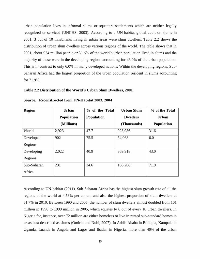
2001, 3 out of 10 inhabitants living in urban areas were slum dwellers. Table 2.2 shows the
distribution of urban slum dwellers across various regions of the world. The table shows that in
2001, about 924 million people or 31.6% of the world’s urban population lived in slums and the
majority of these were in the developing regions accounting for 43.0% of the urban population.
This is in contrast to only 6.0% in many developed nations. Within the developing regions, Sub-
Saharan Africa had the largest proportion of the urban population resident in slums accounting
for 71.9%.
Table 2.2 Distribution of the World’s Urban Slum Dwellers, 2001
Source. Reconstructed from UN-Habitat 2003, 2004
Region Urban
Population
(Millions)
% of the Total
Population
Urban Slum
Dwellers
(Thousands)
% of the Total
Urban
Population
World 2,923 47.7 923,986 31.6
Developed
Regions
902 75.5 54,068 6.0
Developing
Regions
2,022 40.9 869,918 43.0
Sub-Saharan
Africa
231 34.6 166,208 71.9
According to UN-habitat (2011), Sub-Saharan Africa has the highest slum growth rate of all the
regions of the world at 4.53% per annum and also the highest proportion of slum dwellers at
61.7% in 2010. Between 1990 and 2005, the number of slum dwellers almost doubled from 101
million in 1990 to 1999 million in 2005, which equates to 6 out of every 10 urban dwellers. In
Nigeria for, instance, over 72 million are either homeless or live in rented sub-standard homes in
areas best described as slums (Omirin and Nubi, 2007). In Addis Ababa in Ethiopia, Kampala in
Uganda, Luanda in Angola and Lagos and Ibadan in Nigeria, more than 40% of the urban
Page 39
24
population lives in over-crowded houses. In Zambia 80% of the housing stock is classified as
informal with Lusaka alone having about 70% of its housing classified as informal
accommodating about 90% of the city’s population and occupying only 20% of the residential
land (CAHF, 2012). In Dar esalaam, Tanzania between 75% - 80% of housing is considered as
slums and in South Africa about 1.1 million households live in informal settlements. The quality
of housing in Burundi is poor. According to the 2006 household survey, 87.5% of households in
Burundi live in houses with mud floor, and roofing is mostly of informal materials; 20.3% of the
homes are roofed with stubble or palm leaves, and 21% are roofed with dry grass or thatch
(CAHF, 2012).
Kenya hosts some of the most dense unsanitary and insecure slums in the world. Yahya and
Nzioki (1993), in their study of informal settlements in Kenya, noted among other things that
slums have been growing in most cities in Kenya at a rate faster than the urban population
growth. Most of the slums in Kenya are found within the capital city, Nairobi which currently
has an estimated population of over 3 million people, 60% of whom are residing in informal
slums. Paradoxically, in terms of actual physical space, those living in informal settlements
occupy only 5% of the city’s residential land (Cohre, 2008). More than 200 informal settlements
in Nairobi are crammed into this tight space accommodating more than half of the city’s
residents (Cohre, 2008). Examples of slum settlements in Nairobi include Kibera, Mukuru Kwa
Njenga and Mathare valley slum. Kibera is one of the largest slum settlement in Africa,
accommodating the largest population density of any slum in Nairobi, where roughly 2500
people live per hectare or per 10,000 square meters of land, that is, on average one person per
every four square meters.
Slums and informal settlements in Nairobi are characterized by inadequate housing manifested
by structures/houses built of temporary materials of mud and wattle or cardboards. Slums in
Nairobi are also characterized by serious environmental degradation, high population densities,
insufficient or non-existent infrastructure services, forced evictions, and extremely or unsteady
incomes of the inhabitants (Kusienya, 2004). However, some slums in Kenya for example,
Mathare and Kibera slums have in the recent past benefited from up- grading initiatives from the
government of Kenya supported by various donor agencies. The slum up-grading projects,
Page 40
25
although not yet completed, have led to the improvement of infrastructure including water
supplies, roads and new conventional housing.
2.3 Housing Finance
Housing finance is interpreted to mean the capital required for the construction of housing or
housing projects, the resources required to acquire or access housing by households or the credit
supplied by financial institutions (UNCHS, 1991). As noted by Diamond and Lea (1992 in
Akinwunmi, 2009), housing finance is a major factor determining the quality and tenure of
housing consumption, the overall financial portfolio of the public and the stability and
effectiveness of the financial system. Stephens (2009) has argued that housing finance has an
important role to play in shaping each country’s wider housing system.
However, due to the huge capital resources required in the construction or acquisition of housing,
many urban households in developing countries are unable to raise housing finance through own
savings and often result to credit financing from financial institutions. The finance markets in
developing countries are, however, characterized by great operational inefficiencies and seldom
serve the needs of the majority of urban population. The finance institutions in these countries
are few, they charge very high interest rates and have high eligibility requirements making them
inaccessible by majority of urban households especially those in the low and middle income
categories.
As observed by Okpala et al (2006), lending by finance institutions in developing countries is
associated with a standard package of terms and conditions which the poor and those with
modest means find it difficult to comply, hence are left out in the allocation of credit financing.
The terms and conditions of lending, for instance, usually specify the contribution of deposit
(down- payment), interest to be charged on loan and whether fixed or variable, the period of the
loan with penalties for early and late repayments; and loan -to- value ratios which specify the
maximum percentage of the loan against a verified value of the dwelling. The terms and
conditions for lending also specify the amount the loan institution is willing to lend in relation to
the borrower’s income. Those able to meet such terms often find they are still excluded from
formal financial services by cost barriers in the form of high interest rates, transaction fees or
substantial minimum requirement for savings balances or loan amounts (MFW4A, 2013).
Page 41
26
Faced with the challenge of accessing housing finance in the formal finance markets, poor and
middle income households in urban areas of developing countries often resort to informal
mechanisms of financing for their housing. Here, many households use a combination of means
which allow them to:
a). Build while they save
b). Save in building and;
c). Earn by building
Building while saving or incremental building is perhaps the most common of these means,
whereby a household will construct and occupy a partly built house and improve and extend it
over time. Such early occupation allows the household to save on rent. In the short- term,
however, the house will most likely be classified as ‘substandard’. Saving in building refers to
building at costs that are well below the market rates through utilizing family labour, self-help
effort, cheap professional help and craftsmen. Earning by building on the other hand is achieved
through renting out part of house which is under construction and perhaps using the money
realized to complete the dwelling (UNCHS, 1991). In addition to these informal financing
mechanisms, poor urban households access funding from a variety of other informal sources
including rotating savings and loan associations, for example, ‘chamas’ (investment groups) in
Kenya and ‘esusu’ in Nigeria, private money lenders, housing saccos and borrowing from friends
and family. The informal funding sources operate on the basis of third party guarantees and rely
on peer pressure to ensure prompt repayment. They are, however, unsecured and lack the
magnitude of accumulation of funds required for large investment (Akinwunmi, 2009).
While the informal finance mechanisms and means have achieved some success in enabling
urban households in developing countries acquire their own homes, the JCHS ( 2005) has noted
that informal finance usually provide slow incremental housing based on retained savings which
is more costly to the end user. “Self-development” by owners using small craftsmen results in
high real resources cost reflecting inflation, a lack of economies of scale and organization
(JCHS, 2005). With the shortcomings of the informal finance mechanisms, there is need to
devise means to expand the supply of formal credit to low and moderate income households.
Page 42
27
There is the need for developing countries to develop effective formal housing finance systems
that will work for all income ranges (JCHS, 2005).
An effective and efficient housing finance system and market channels resources to support
housing demand, allowing households to accelerate purchase and construction of housing and
facilitates a better allocation of resources between housing, other goods and savings over the life
cycle. An effective housing finance system also makes housing loans available to qualified
borrowers without excessive wait, provides loans whose relative cost is in line with the cost of
credit in the economy generally, and reflects the risks of the investment (JCHS, 2005).
2. 3.1 Forms of Housing Finance
There are two main forms of financing for housing, namely; debt finance and equity finance.
2.3.1.1 Debt Finance
Debt finance can be classified into short-term and long- term finance
Debt finance from micro-finance institutions are usually short-term construction loans with high
interest rates and are less appealing for housing acquisition and construction (Nubi, 2005). The
most popular funding instrument for housing is the long term loan. Here, a specified maturity
date sets the time for repayment of the loan amount and interest. Term loans vary from short-
term (bridging finance, working capital, trade finance) through the medium term (two to five
years for working capital) to long-term (project finance, capital expenditure) which might have a
tenure of between 10 and 30 years (Heffernon, 2003 in Akinwunmi 2009). Lending for
commercial purposes are short-tenured while the typical tenure of mortgage loans varies between
10 years to as long as 30 years.
2.3.1.2 Equity Finance
Equity finance consists of all monies pulled together from friends, relatives or business entities
who are interested in maintaining interest in the house purchased with the money raised. The
most common equity-financed model for housing is the Real Estate Investment Trust (REITs).
The REITs structure is designed to provide a similar structure for investment in real estate as
mutual funds provide for investment in stocks. The concept of REITs began in the United States
Page 43
28
in the 1960s but became popular in early 1990s (Seiler and Seiler, 2009). REITs started in
Australia as listed property Trusts (LPTs) since 1970 and in January 2007, REITs were
introduced in the United Kingdom with Germany and Italy also introducing REITs in 2007. In
Kenya, the Capital Market Authority (CMA) has already designed and formulated regulations to
guide investment in REITs and the necessary regulations and legislation have been approved by
parliament.
2.3.2 Sources of Housing Finance for Lenders
The dominant source of funding for housing (mortgage) finance in both the developed and
developing countries is the customer savings deposits. This funding mechanism, however, has
the short-coming in the sense that customer deposits being short- term liabilities can be
withdrawn at any time, and, are therefore not appropriate funding source for long - term illiquid
assets, like mortgages.
According to the commercial bank loan theory, banks should not grant long - term loans such as
housing/ real estate loans or loan for financing purchase of plant and machinery because they are
considered too illiquid. Shin (2009) has observed that within a financial system where short-
term liabilities are being used to acquire long- term illiquid assets, any disturbance in the
leverage level (ratio of total assets to equity) has to show up somewhere within the financial
system. Given that short-term liabilities can be withdrawn at any point in time, financial
institutions relying on short-term liabilities to fund long term illiquid assets are likely to face a
liquidity crisis (Shin, 2009).
However, despite the short-coming in utilizing deposits liabilities to fund long term mortgage
loans, Cho (2007) has observed that a large percentage of financial institutions in developing
countries are still relying on short- term deposits to fund long-term mortgage assets.
There is, therefore, the need for financial institutions and banks in developing countries to pursue
alternative sources of funding long-term illiquid assets like mortgages. Secondary mortgage
markets offer an important alternative source of long term funding and have largely been utilized
in the developed countries as a source of funding for mortgages. Secondary lenders source long-
term funds from the international investment markets and also from local institutional investors
which they lend to commercial banks who then lend to individual borrowers at competitive
Page 44
29
interest rates. Secondary lenders also source long term funds from the capital markets.
Specifically, secondary lending institutions buy the mortgage assets of loan originating banks
and issues securities in the capital markets which are backed or secured by those mortgages in
what is referred to as mortgage backed securities (MBS). Mortgage backed securities (MBS) are
investments similar to stocks, bonds or mutual funds, whose value is secured or backed by the
value of an underlying bundle of mortgages.
With a well functioning secondary mortgage market, commercial banks do not have to hold
mortgages until maturity since they can sell them to the secondary lending institutions and this
effectively enhances the liquidity of the loan originating banks thus enabling them to lend to
many borrowers at affordable interest rates (Ergungor, 2008). There is, however, no efficient
secondary mortgage market in developing countries and this puts enormous pressure on housing
finance institutions and banks to carry mortgage loans to maturity and this limits the ability of
the banks to originate more loans and at affordable interest rates (EFInA, 2010).
Besides customer deposits and securitization, there are other innovative ways of mobilizing long
term funds in order to improve the supply of housing finance in developing countries. These
innovative finance products include; Issuance of Diaspora Bonds, Migrant Remittances, Pension
Funds and Bonds, Mortgage Liquidity Facility (MLF) and Insurance Life-funds. These are
briefly discussed below:
i) Issuance of Diaspora Bonds
A Diaspora Bond is a debt instrument issued by a country or a private corporation to raise
financing from its citizens in a foreign country. Several countries have used this method to raise
long-term funds for example, India and Israel raised US dollar 11 million and 25 million,
respectively from diaspora bonds (Ratha et al, 2008). In 2006, the South African government
issued a reconciliation and development bond targeting their citizens abroad. Ghana sold a
golden jubilee savings bond to Ghanaians in Europe and the United States and Kenya launched
its form of Diaspora bond in 2008.
Diaspora bonds have that selling point of the desire by the residents abroad of the need to
contribute to the development of their home country. It is an alternative to investing directly in
their countries of origin. However, despite the potential market for Diaspora bonds, some of the
Page 45
30
countries in the developing world are still struggling with weak and non-transparent legal
systems for contract enforcement and lack of effective regulations on their financial
intermediations (Akinwunmi, 2009)
ii) Migrant Remittances
Remittances are defined as the sum of workers’ remittances, compensation of employees and
migrant transfer (World Bank, 2007). Remittances are considered as a stable source of external
finances that can be effectively utilized for development purposes, one of which is housing
finance that requires long-term funding. Remittances to developing countries have increased on
average by 16% in annual terms since 2000 (Gupta et al, 2009). As at 2006, the total remittances
to Sub-Saharan Africa countries stood at US dollar 9 billion having grown from US dollar 8
billion in 2004. Remittances to developing countries increased by 12.5% in 2011 to US dollar
355 billion from US dollar 316 billion in 2010 (CBK, 2013). In Kenya, remittances in 2013 rose
to US dollar 1.29 billion (Kshs. 110.76 billion) from US dollar 1.17 billion (Ksh. 100.4 billion)
recorded in 2012 (CBK annual reports, 2012& 2013).
iii) Bonds and Pension Funds
Many countries in developing world have a relatively advanced bond markets. In South Africa
and Nigeria, for example, there is a well developed market for government securities and
corporate bonds have seen significant growth in recent years (Blommestein and Horman, 2007).
In 2008, the Federal Government of Nigeria raised US dollar 400 million from the capital market
to finance affordable housing projects.
There is also increasing utilization of pension funds to finance long-term developments like
housing. Most developing countries including Kenya have enacted legislation to allow use of
pension funds to finance mortgages.
iv) Mortgage Liquidity Facility (MLF)
A mortgage liquidity facility (MLF) is a finance institution that re-finances the mortgage
portfolio of primary lenders. A mortgage liquidity facility improves the liquidity of participating
banks and enables them to lend to many borrowers and at competitive interest rates. Many
countries in the developing world have already set up MLF. A good example is the Tanzania
Page 46
31
Mortgage Re-Finance Company (TMRC) that was established in 2010. This World Bank
supported MLF had financed 636 mortgages in Tanzania by October 2012 (CAHF, 2013).
Egypt’s mortgage liquidity facility launched in 2006 increased the total mortgages to 29,631 by
2011. In Togo, a regional mortgage liquidity facility- the Caisse Regional de Refinancement
HypotheCaire, was created in 2012 to promote easy access to long-term financing for
commercial banks to enable them to finance housing loans. The Nigeria government is working
with the World Bank to develop a mortgage liquidity facility which is expected to increase
mortgages to 200,000 in the next 5 years (CAHF, 2013). Kenya does not have a mortgage
liquidity facility
v) Insurance Life -Funds
Life funds of insurance companies are long- term savings in form of annuities or endowment
policies, which can only mature at the occurrence of certain events, which might be at death,
accident, retirement or at maturity. Life funds are not only long-term savings but relatively
cheaper than deposits (Pilbeam, 2005). Therefore Insurance companies have funds appropriate
for financing housing construction and other long-term investments. However, as Anderson et al
(2009) has aptly observed, insurance companies are traditionally the most conservative lender to
housing and real estate. In Kenya, lending by the insurance companies is regulated by the
Insurance Act and the Insurance Regulatory Authority (IRA) which limits the amount of assets
of insurance companies that can be lend for housing.
2.3.3 Housing Finance Markets in Developing Countries
While in developed countries, housing finance markets are large and well developed, the markets
in most developing countries are in the developing stages and others in their infancy stage. In
countries like Britain, Denmark and the United States, outstanding mortgage loans are almost
equivalent to their gross domestic product (GDP) (Akinwunmi, 2009). In 2006, mortgage
outstanding as a percentage of GDP was 86% in the United States, 72% in the United Kingdom
and 90% in Denmark. The minimum ratio for any of the developed economies is Germany which
had a ratio of 52% of GDP (Saravanan, 2007).
In contrast, however, the size of mortgage markets in developing countries is quite small
compared to counterparts in developed economies. As shown in Table 2.3, outstanding mortgage
Page 47
32
debt to GDP in most countries in Africa except South Africa, Namibia and some economies in
North Africa is less than 5% and some even less than 1%.
Table 2.3: Mortgages as a Per cent of GDP in Selected African Countries
Source: CAHF (2013)
Country Total Mortgages as a % of
GDP
Year
Central African Republic 0.07 2005
Senegal 0.07 2005
Mozambique 0.14 2008
Burkina Faso 0.29 2013
Tanzania 0.32 2013
Nigeria 0.38 2013
Ghana 0.45 2013
Cameroon 0.5 2005
Malawi 0.51 2013
Uganda 0.98 2013
Egypt 1 2011
Zimbabwe 1.15 2012
Algeria 1.19 2013
Burundi 1.2 2013
Zambia 1.53 2012
Kenya 1.88 2013
Botswana 2.29 2013
Rwanda 2.3 2010
Tunisia 9.25 2013
Mauritius 12.99 2011
Morocco 13.85 2013
Namibia 18.21 2011
South Africa 33.9 2012
Page 48
33
As at December 2013, total mortgages as a percentage of GDP was 0.29 in Burkina Faso,
0.32% in Tanzania, 0.38% in Nigeria and 0.45% in Ghana. Total residential mortgage
portfolio in Uganda was estimated at 0.98% while in Kenya, the ratio of mortgage debt to
GDP was 1.88%. South Africa and Namibia are the market leaders for Sub- Saharan Africa
with ratios of 33.9 % and 18.21% respectively.
South Africa has a fairly well developed finance sector compared to regional standards. The
country has 32 registered banks of which 4 dominate the mortgage market. There is also a
small but growing housing micro- finance sector who lend micro loans to borrowers seeking
to improve their housing. The 1994 South Africa housing policy implemented measures to
enhance access to housing finance which saw the establishment of the National Housing
Finance Corporation (NHFC) of South Africa.
In Namibia, there are 4 commercial banks, one savings bank, 10 insurance companies and
348 micro- lenders. In recent years, there has been an increase in bank lending to households
and corporations with about 40% of these loans being in the form of mortgages. Namibia’s
mortgage market is currently 18% of GDP which is relatively high by African standards and
second only to South Africa. Mortgage finance is also available from informal housing
finance services supported by NGOs and other informal savings groups including money
borrowed from friends and relatives.
In Nigeria, despite the size of its economy, mortgage debt to GDP is very small at 0.38 as at
December 2013. Only about 5% of the 13.7 million housing units in Nigeria are financed
with a mortgage (CAHF, 2013). Most residential mortgage loans are provided by the
commercial banks, primary mortgage institutions (PMIs) and some institutional employers.
Mortgage lending in Nigeria is constrained by several factors, among them the limited
availability of long- term funds, weak capital base of the PMIs, difficulty in accessing land
and secure title partly due to the mandatory governor’s consent for all land transactions, in
adequate legal framework and poor housing market infrastructure (EFInA, 2010). The high
mortgage interest rates in Nigeria currently between 18-24% undermine housing finance
affordability and access to mortgage finance (CAHF, 2012). Informal housing finance
sources are however available provided by the esusu (rotating savings and loan
Page 49
34
associations), traditional co-operative system, private money lenders, credit cooperatives,
individuals and family savings (EFInA, 2010).
Ghana’s finance sector comprises of 29 banks, a stock exchange, pension firms and micro
finance sector which offer housing micro-finance. The Ghanaian mortgage market is
however small with mortgages outstanding at 0.45% to GDP in 2013. There are five major
players within the Ghanaian mortgage market. These banks offer a variety of mortgage
products including mortgages for home purchase, improvement or completion of homes, as
well as home equity mortgages. The mortgage market in Ghana is constrained by
cumbersome property registration process which remains manual and fraught with
administrative limitations, lack of titled land also inhibit development of the mortgage sector
(CAHF, 2012).
In Angola, access to banking finance is for the privileged few, with only 8% of the
population using the formal financial system. As of 2011, there were 23 banks with
significant concentration among just a few banks. There is however, growing interest in the
mortgage market with one bank, Banco Africano de investimento (BAI) currently offering
loans of up to 20 years, financing up to 85% of the value of the property. The micro- finance
sector in Angola is still under-developed. Mortgage lending in Angola is constrained by
among other factors, lack of access to a well developed credit information system (CAHF,
2012).
Zambia’s mortgage market is quite small. Only a few of the commercial banks offer
mortgage finance. The sector is however growing rapidly. In 2012, the mortgage loan
portfolio stood at about US dollar 239.3 million having increased by more than 50% as at the
2011 figure (CAHF, 2012). A key challenge for residential mortgage lenders in Zambia is
access to funding as the whole- sale finance sector and capital markets remain undeveloped.
Mortgage interest rates offered by commercial banks and building societies are high. The
average interest rate by the commercial banks in 2011 was 18.8% for a 24-year mortgage
loan. Building societies’ interest rates are higher at 20% and above.
Burundi’s housing finance sector has grown over the last 5 years. The mortgage portfolio
has increased by over 150% from US dollar 1.17 million in 2007 to US dollar 3.54 million in
Page 50
35
2010. As a percentage of GDP, however, the housing finance sector is insignificant by
regional standards. In 2010, the number of mortgages in the market were estimated at about
350, and the average size of a mortgage was US dollar 10,000. By 2011 and mid 2012, the
total number of mortgages issued by the financial institutions was estimated at about 500
targeting only high income earners. A major challenge in providing mortgage finance in
Burundi is the lack of long term funding schemes within the domestic banking system and
lack of a developed pensions and insurance industry which are crucial in resource
mobilization and maturity transformations. Other challenges include the high prices of
houses (CAHF, 2012 & 2013).
In Rwanda, the banking system comprises of 14 financial institutions as listed by the
National Bank of Rwanda, up from 11 in 2011. Mortgage lending accounts for about 15-
20% of the country’s US dollar 70 billion loan book, and the value of mortgages to GDP
stood at 2.3% in 2010. Informal house finance sector in Rwanda comprises Sacco’s and
there are 88 licensed Sacco’s and micro-finance institutions (MFIs) as of march 2012. A
major challenge to mortgage lending in Rwanda is lack of liquidity for long – term finance
for mortgages as well as for micro - finance institutions. The Rwandan mortgage market also
lacks a good source of credit information. The existing public credit registry does not have
sufficient coverage as it covers only 0.7% of the adult population. There are no private credit
reference bureaus in Rwanda (CAHF, 2012).
Tanzania’s house finance market is the smallest in the East African region. The value of
mortgages outstanding to GDP stood at 0.32% in 2013. Mortgage lending in Tanzania has
over the years been constrained by a poor land tenure system and a weak capital base of the
lenders. As at 1995, Tanzania had only provided 14,000 mortgages through the collapsed
Tanzania Housing Bank. However, recently, important development in the mortgage
industry is the establishment of the Tanzania Mortgage Refinance Company (TMRC).The
TMRC is a Mortgage Liquidity Facility (MLF) established by the Government of Tanzania
with the support of the World Bank, and created as a private sector institution owned by the
banks with the sole purpose of supporting banks to do mortgage lending by refinancing the
banks’ mortgage portfolios. The TMRC serves as an important source of long - term funding
at attractive interest rates. Funding raised through TMRC is charged at 10% interest which
Page 51
36
translates into 13% on mortgages supported with the TMRC, while other lenders who do not
have a stake in the TMRC charge 19 -20% interest on mortgage loans (CAHF, 2012). There
are also informal housing finance sources in Tanzania supported by Saccos and NGOs which
cater for the low income categories.
In Uganda, the banking sector continues to grow. The number of commercial banks has
increased to 23, with 3 licensed credit institutions and only 4 licensed micro-finance
institutions. Only 9 financial institutions in Uganda offer mortgage finance of which 5
dominate. With interest rates above 15% as at 2012, mortgages remain expensive, and the
residential mortgage sector mainly serves middle and high level income earners. The ratio of
understanding mortgage debt to GDP was at 0.98% as at December 2013(CAHF, 2013)
Kenya’s financial system is relatively well developed but remains vulnerable to considerable
government influences and weaknesses in the supervisory regime (MFW4A, 2013).
According to the Central Bank of Kenya (CBK) annual reports of 2012 and 2013, the
financial system in Kenya consists of the Central Bank of Kenya (CBK) as the regulatory
authority, 44 banking institutions (43 commercial banks and 1 mortgage finance company-
MFC), 5 representative offices of foreign banks, 8 deposit taking micro-finance institutions
(DTMs), 2 credit reference bureaus (CRBs) and 112 forex bureaus (FXBs). The finance
system in Kenya also comprises of 42 insurance companies and the Nairobi Securities
Exchange (NSE) which has 50 listed firms across the financial, industrial, commercial and
agricultural sectors). Pension firms also form part of the Kenya financial system.
Kenya has a fairly dynamic mortgage industry compared to counterparts in the East Africa
region, but quite low by international standards. The ratio of mortgages outstanding was at
1.88% of GDP as at December 2013 having declined from 2.51 % as at 2012. There were
19,177 mortgage loan accounts in the market in December 2012 up from 16,029 in 2011
(CBK, 2012). The average mortgage loan size increased from kshs. 5.6 million in 2011 to
kshs. 6.4 million in 2012 (CBK, 2012). The increase was attributed partly to increase in
property prices.
Page 52
37
Despite the high number of financial institutions offering mortgages in Kenya, about 71%
of lending to mortgages market was by 5 institutions .The same institutions dominated the
mortgage market on the 2011 CBK mortgage survey (CBK , 2011).
The main providers of mortgages in Kenya are the Housing Finance (HF) Limited, the
Kenya Commercial Bank (KCB), CFC Stanbic Bank, Standard Chartered Bank (SCBK) and
the Barclays Bank of Kenya (BBK) Limited. According to the CBK annual reports of 2011
and 2012, Housing Finance (HF) Limited was the mortgage market leader both in terms of
value of mortgage loans and number of customers in 2011. In 2012, Housing Finance (HF)
maintained the lead in terms of number of mortgage customers, but Kenya Commercial
Bank (KCB) led in terms of the value of mortgages outstanding.
As shown in Table 2.4, mortgage customers for Housing Finance (HF) Ltd stood at 5,235 in
2012 compared to Kenya Commercial Bank (KCB) whose total mortgage accounts were
5,091. The value of mortgages for Housing Finance (HF) was however slightly below at
Kshs. 30 billion compared to KCB at kshs. 31 billion.
Table 2.4: Number of Mortgage Accounts and Mortgages Outstanding in 2012
Source: CBK (2012)
Bank No. of
Mortgage
Accounts
% of
Total
Value of Mortgages
Outstanding
(Kshs in Billions)
% of
Total
Housing Finance (HF) 5,235 27.3 30.3 24.7
Kenya Commercial Bank (KCB) 5,091 26.5 31.5 25.6
Standard Chartered Bank (SCB) 1,480 7.7 9.7 7.9
CFC Stanbic Bank (CFC) 1,340 6.9 9.5 7.7
Barclays Bank of Kenya (BBK) 1,021 5.3 4.3 3.5
Equity Bank Ltd (EBL) 702 3.6 3.7 3
Development Bank Ltd (DBL) 579 3 2.6 2.1
Consolidated Bank Ltd 566 2.9 3.8 3.1
Co-operative Bank 398 2 6.6 5.4
Others 2,765 14.8 20.4 17
Total 19,177 100 122.2 100
Page 53
38
Various factors have militated against mortgage lending in Kenya, among them is the high
interest rates charged by banks and financial institutions. High interest rates for the first half
of 2012 impacted negatively on the mortgage market performance in Kenya and this saw
Non Performing Loans (NPLs) increasing from kshs.3.6 billion in December 2011 to kshs
6.9 billion in December 2012(CBK, 2012).
The interest rates charged on mortgages in Kenya were on average 18% in 2012 and ranged
from 11% - 25%. In 2013, interest rates on mortgages averaged 16.89% and ranged from
between 15.5% - 19% (CBK, 2012, 2013).
Other factors that have constrained the performance of the mortgage market in Kenya as
identified by CBK (2012) include the following:
-Stringent lending requirements by banks
- Lack of long- term funds for lending
- Low level of income
- Credit risk (limited credit histories, documented income)
-Lack of understanding of mortgage products by consumers
-Burden of regulation (prohibiting capital reserve requirement, liquidity rules by the
regulatory authority which limits number of banks in the industry.
-High cost and time of foreclosing on a property
- Difficulties with property registration/titling
- Lack of capacity/ skills in banking sector to develop attractive mortgage products,
- AIDS/HIV as an inhibitor of long- term lending.
2.4 Housing Affordability
While there is no single agreed definition of housing affordability, the term refers broadly to a
person’s ability to pay for their housing (O’Flynn, 2011; Bujang et al, 2010). It is a tenure-
Page 54
39
neutral term. By this it means that it relates to both home-ownership affordability and rental
market affordability. In this study, however, the term is used within the context of home
ownership affordability.
According to Gabriel et al (2005), one of the most helpful statements about what housing
affordability entails was provided by MacLennan and Williams (1990) in stating that;
‘Affordability’ is concerned with securing some given standard of housing
(or different standards) at a price or rent which does not impose, in the eyes
of some third party (usually government), an unreasonable burden on
household incomes’.
A research for the Australian Housing and Urban Research Institute (AHURI) cited in O’Flynn,
(2011) considered housing affordability to be;
‘An expression of the social and material experiences of households, in relation to
their individual housing situations. Affordability expresses the challenge each
household faces in balancing the cost of their actual or potential housing, on the
one hand, and their non-housing expenditures, on the other, within the constraints
of their income’
The Australian government’s National Housing Strategy (NHS) cited in Yates et al (2007)
defines affordability as;
‘The notion of reasonable housing costs in relation to income,that is, housing costs
that leave households with sufficient income to meet other basic needs such as food,
clothing, transport, medical care and education.’
In New Zealand, housing affordability is defined as;
Page 55
40
‘The ability of households to rent or purchase housing in an area of choice at a reasonable
price, the capacity of households to meet on going costs, and the degree that
discretionary income is available to achieve an acceptable
standard of living.’ (Yates et al, 2007).
Bramley (1990 in Mostafa et al, 2005) has specified that ‘households should be able to occupy
housing that meets well established (social housing) norms of adequacy (given household type
and size) at a price or rent which leaves them enough income to live on without falling below
some poverty standard’.
A household is said to have a housing affordability problem if after paying for housing services it
is left with insufficient income to enable it meet its other basic needs.This expression agrees with
the definition of affordability as given by the Australian National Housing Strategy (NHS) as
stated above, which emphasize the need for households to pay for housing at costs which leaves
them with sufficient income to pay for other household basic needs.
Affordability is, therefore, expressed as the relationship between housing expenditure and
household income and establishes a standard in respect of which the amount of income spent on
housing is deemed unaffordable. The standard is defined in terms of an absolute residual income
once housing costs have been met, or as a ratio measure specifying the acceptable proportion of
household income to be spent on housing.
In the section below, the various approaches to measuring affordability are discussed. The main
approaches are the ratio and the residual measures. As noted in the discussion, the ratio measures
are the simplest and most explicit approaches to measuring affordability and have been adopted
in this study as the appropriate definition and measurement of housing affordability in the home
ownership mortgage housing sector in Kenya. Specifically, the simple housing cost-to- income
ratio has been adopted as the appropriate measure of affordability of the households considered
in the study.
2.4.1 Affordability Measures
There are two main approaches to measuring affordability. These are:
Page 56
41
i. Ratio measures
ii. Residual measures
2.4.1.1 The Ratio Measures
Ratio measures are the most commonly used measures of housing affordability. The approach is
variously referred to as; housing expenditure- to- income ratio, house purchase-to- income ratio
or simply the housing cost approach. The ratio approach conceives housing affordability as a
measure of the ratio between what households pay for their housing and what they earn. In
simple terms, the ratio is an expression of the relationship between household’s income and
housing expenditure and indicates the proportion of family income that goes into the payment for
their housing (Bujang et al, 2010). In the home ownership (mortgage) housing sector, the ratio is
the proportion of the household’s income that goes into repayment of the mortgage loan.
There are two main derivatives of the ratio measure, these are;
a).The simple “housing cost to income” ratio
b). Fixed ratio with benchmarks/ rule of thumb standard.
Simple Housing Cost - to - Income Ratio
This simply indicates the proportion of household income being dedicated to housing. A higher
ratio indicates the household is spending too much of its income on housing while a lower ratio
shows the household is spending little on housing. Other factors held constant, households with
higher ratios are likely to experience affordability problems compared to those with lower ratios
because such households will have little income remaining for other basic needs after paying for
their housing. A household with a ratio of say 10% for example, is considered to have better
affordability (less affordability problem) compared to another with say a ratio of 40%.
Simple ratios can, therefore, be used to monitor shifts in affordability of households over time.
They can also be used to tell whether the affordability of a household is improving or worsening
(Gabriel et al, 2005). Simple house cost -to- income ratio can also be used to compare the
affordability levels of different households.
Page 57
42
While simple ratios are useful in tracking shifts in affordability, they do not provide a clear
rationale for policy intervention. In order to make such ratios more responsive to policy
objectives, ratio measures have been linked to a normatively ascribed affordability benchmark or
rule of thumb standard. The affordability benchmark is used to determine the point at which
affordability is deemed to be a problem for the average household and which in turn require
some form of policy intervention (Gabriel et al, 2005). The affordability benchmarks and rule of
thumb standards are discussed below under the fixed ratio approach.
Fixed Ratio with Benchmark
Under the fixed ratio approach, households are said to have unaffordable housing if their housing
costs (e.g. mortgage payments) take up more than some pre-determined proportion of their
income. The fixed ratio approach specifies the acceptable maximum proportion of households’
income to be spent on housing, beyond which housing will be regarded as unaffordable
(Johnston, 2008). Usually a “ rule of thumb” standard of no more than 25% or 30% of
households monthly income being spend on housing costs is deemed appropriate and affordable
(Stone, 1993 in Okechukwu, 2009). This rule of thumb standard has been used by mortgage
credit institutions in their risk assessment of potential customers. The ratio has also been used by
the World Bank, United Nations Development Programme and the United Nations Human
Settlement Programme in their urban management programmes.
However, despite the use of the ratio approach, critics have expressed concerns about setting the
affordability benchmark at a particular level without any clear, scientific rationale (Free man et
al, 2000). Various scholars have specifically questioned about the application of the 25 or 30%
affordability benchmarks. Stone (1993 in Nelson et al, 2002) has for instance argued that high
income and small households can afford to spend much more than 30% of their income on
housing and still have enough income left over to satisfy other basic needs. Conversely,
extremely low income and large households that pay even 10% of their income on housing costs
may be forced to forego essential medical care, health and food. The ratio, therefore, has a
tendency to under- estimate the affordability problems of lower income households and over-
estimates the problems of high income households.
Page 58
43
Other limitations of the ratio approach is that the ratio does not control for changes in housing
quality and the impact of expected appreciation in cost of housing over time; it fails to account
for the actual financial constraints that may be faced by home-owners; and that the ratio does not
account for differences in household sizes, household types, and locational variations in income
and mix of homes available for sale; neither does it discern cases of high house price to income
ratio that may be due to a preference for high housing consumption (Burke and Ralston, 2003).
There are, however, some advantages in the use of the ratio, which have sustained its popularity
over the years and its continued use especially for policy and research. The ratio, for instance, is
easy to calculate and to interpret and can easily be understood by non- experts; the data required
for calculating the ratio are also readily available from official sources in many countries; the
ratio is amenable to use in comparative studies across different areas and over different periods;
and as has been observed by Bogdon and Can (1997 in Okechukwu, 2009), if used in
conjunction with other affordability measures, the house price- to- income ratio has the potential
to provide a useful starting point to examine housing affordability problems.
2.4.1.2 Residual Measures
Residual measures are variously referred to as “after poverty”, “non- shelter first”, “shelter
poverty”, “living standard measures” or simply basic non-housing cost approach. Residual
measures conceive housing affordability from a basic non-housing consumption perspective. The
measures are concerned with the relationship between housing costs and the capacity of a
household to maintain an acceptable standard of living after paying for the cost of their housing
(Johnston, 2008).
According to Milligan (2003 in Gabriel et al 2005), residual measures focus on the income
remaining after housing costs are met and considers whether housing is affordable in the context
of current income levels and essential household expenditure. Under the residual approach, a
household after paying for housing should be left with adequate residual income that enables it to
comfortably meet other household basic necessities such as food, clothing, health and education.
Stone (1993 in Okechukwu, 2009) argue that since housing costs generally make the first claim
of a household’s disposable income with non-housing expenditure having to be adjusted to
Page 59
44
whatever remains of the income, the most a household should be required to pay for housing is
that which leave it able to meet non-housing basics at a minimum level of adequacy. A
household is, therefore, paying more than it can afford for housing if after paying for housing, it
is left with insufficient income to meet other basic household needs.
Residual measures thus entail establishing the minimum residual income that will enable
households to sustain an acceptable standard of living. The acceptable residual income to
guarantee minimum standard of living after paying for housing is determined using either the
poverty line approach or the budget standards approach. Under the poverty line approach,
residual incomes are linked to the official poverty line thresholds as defined by countries for
specific localities or regions. Budget standards are also prepared for countries and can also be
used to define the minimum residual income for households. Budget standards determine the
acceptable minimum standard of expenditure consistent with a modest budget (Burke, 2003).
According to Saunders et al (1998b), a budget standard for a country sets to represent what
households’ needs in a particular place at a particular point in time, in order to achieve a specific
standard of living.
Yates and Gabriel (in O’Flynn 2011), consider the main advantage of residual measure to be its
ability to consider the impact of household structure on household needs by taking into account
differences in non-housing needs for different household types. However, they emphasize that
this is also a weakness of the measure because it requires a judgment (sometimes subjective) to
be made as to what these non-housing needs are. A perceived further weakness of the residual
measure is that it imposes “more onerous data requirements” and can be complex and time
consuming.
2.4.1.3 Other Measures
Although the ratio and residual measures are the most common approaches to measuring
affordability that have been identified in the literature, there are also other measures of
affordability which needs to be mentioned. There is for instance, the Accessibility/Deposit Gap
Method which only applies to measurement of home-ownership affordability. The method
attempts to measure the savings/deposit required to purchase a home and the ability of the
purchaser to secure the necessary mortgage for the purchase. As noted by smith (in O’Flynn
Page 60
45
2011), this is often seen as the difference between house prices and the maximum borrowing
capacity of households, or the gap that needs to be made up by a deposit. The other approach of
measuring affordability is by comparing house price with incomes. That is, you compare the rate
of increase of house prices with rate of increase in incomes and see whether affordability is
increasing or decreasing.
2.4.2 Housing Affordability Problems in Developing Countries
Access to adequate and affordable housing is a current and growing problem in almost all
countries in Africa. According to the UN-habitat (2011), housing problems are largely to do with
affordability. Housing is expensive and incomes are too low. The inputs to housing are too
expensive especially land, finance and building materials. Land supply is insufficient, is poorly
serviced and lacks security of tenure. Conventional housing finance in the developing countries
of Africa is underdeveloped and inflexible and seldom serves households in low and middle
income categories. While microfinance and community based savings groups are providing
alternative housing finance, they remain constrained by unsupportive institutional and regulatory
frameworks (UN- habitat, 2011).
According to the World Bank (2007), only 3% of the entire population in Africa has income
viable for a mortgage. The Africa Development Bank (AFDB) estimates that just under 20% of
the African population earns more than US dollar 20 per day and 36.5% of the population live
below the international poverty line of US dollar 2 per day (AFDB, 2011).
House prices in Africa are too expensive. Data from selected countries on the cheapest newly
built house by a formal developer show that in 2013, the cheapest house for sale in Mali was US
dollar 5,800 (excluding land), US dollar 13,300 in Egypt, US dollar 28,000 in Tanzania, and US
dollar 50,000 in Gambia. In Kenya, the price of the cheapest newly built house by a formal
developer in 2013 was US dollar 18,000 (CAHF, 2013).
In order to conceptualize the nature and extent of affordability problems of households in
developing countries of Africa, the relationship of house prices to the purchasing power of
individuals in these countries is analyzed. In Table 2.5 and Graph 2.0, the Gross National Income
(GNI) per capita taken as a very loose indicator of income per country per person is plotted
against the 2013 house prices in selected African Countries. The Gross National Income (GNI)
Page 61
46
per capita 2013 figures are obtained from World Development Indicators data base by the World
Bank.
Table 2.5. Relationship of Income to House Price in Selected Countries in Africa
Note: GNI per capita and House price figures quoted are for year 2013 except Rwanda,
whose figures for 2013 are not available
Source: CAHF (2013), World Bank, 2014
Country GNI per capita 2013 figures(
in US dollar)
Price of cheapest newly built
house by a formal developer
in 2013(US dollar)
Ethiopia 470 68,000
Gambia 510 50,000
Nigeria 2760 18,000
Algeria 5290 32,000
Egypt 3160 13,000
Ghana 1760 25,000
Botswana 7,730 58,000
Rwanda 800 (year 2012) 79,000(year 2012)
Tanzania 630 28,000
Kenya 930 18,000
Burundi 280 19,000
Uganda 510 28,000
South Africa 7,190 24,000
Mali 670 5,800
Page 62
47
Graph 2.0 Relationship of Income to House Prices in Selected Countries of Africa
Source: CAHF, 2013
Table 2.5 and Graph 2.0 shows that in Ethiopia, the cost of the cheapest newly built house of
125m2 in floor area is US dollar 68,000. A buyer ordinarily would deposit 10% of this amount
(i.e. US dollar 6800). To afford a mortgage for the difference at current interest rate of 9.5% over
a 20 year period, the buyer would have to earn US dollar 2061 per month ( CAHF, 2013). Such a
house is however unaffordable to the majority, as 66% of Ethiopians live on less than US dollar
60 per month. The income per capita is also very low at US dollar 470 (World Bank, 2014)
Housing development in Gambia is targeted at the high income market. The houses are large
measuring approximately 225m2 and are very expensive starting at US dollar 50,000 for a two
bedroom house. Most Gambians cannot afford this house, as majority about 55.9% live on less
than US dollar 60 per month (CAHF, 2013). The income per capita is also low at US dollar 510
(World Bank, 2014). Majority of Gambians self- build their housing incrementally.
In Ghana, the cheapest newly built house for sale is US dollar 25,000 and measures roughly
75m2. A buyer has to put down US dollar 2500 deposit and earn US dollar 970 a month to afford
a 20 year mortgage at 13.5% interest rate. Most Ghanaians, however, are poor with 51.8% living
below the international poverty line of less than US dollar 2 per day. The cheapest newly built
house in Mali is US dollar 5,800, plus another us dollar 1,000-4,000 for the land, depending on
the location. This is however far beyond the affordability of the majority with about 78.66% of
Malians living on less than US dollar 2 per day. In Nigeria, a household earning a minimum
Page 63
48
wage of US dollar 116 per month could only afford to borrow US dollar 4,685 which is not
enough for the cheapest house, which is at US dollar 18,000 costing almost 4 times that amount
(CAHF, 2013). About 78.4% of Nigerians live on less than US dollar 60 per month.
In South Africa, according to the World development indicators by the World Bank, Gross
National Income(GNI) per capita in 2013 was US dollar 7190, and with the entry level house at
US dollar 24000, only about 15% of the population can afford it. In Algeria, the cheapest newly
built house measuring 75m2 is US dollar 32,000 and is only affordable to the top tiny minority.
The bulk of the population in Algeria about 72% earns between US dollar 2-10 per day (CAHF,
2013). Most developers in Rwanda build homes priced about US dollar 100,000, affordable to a
tiny majority as 82.4% of Rwandese live on less than US dollar 60 per month. The income per
capita is also low at US dollar 800. In Tanzania, 87.9% live on less than US dollar 2 per day.
Housing is unaffordable to the majority as the cost of the cheapest house for sale is US dollar
28,000.
In Burundi, the cheapest newly built home measures approximately 125m2
and sales at US dollar
19,000, affordable to less than 5% of the population. Most Burundians self build and incremental
construction is the dominant form of house construction (CAHF, 2013). About 93.4% of the
population in Burundi lives below the international poverty line. To buy the cheapest house in
Uganda, a household would spend US dollar 32,000 including the costs of transfer, legal charges
and taxes; the borrower has to pay a deposit of US dollar 6,400-9,600, which is far beyond most
households, as about 64.7% live below the poverty line. High interest rates in Uganda over 18%
in 2012 compromises loan affordability. Stringent loan requirements for example, deposit
requirement that range from 20%-30% further restricts mortgage affordability (CAHF, 2013).
In Kenya, 67.2% live below the international poverty live. High interest rates undermine
affordability even for modestly priced housing. Interest rates in 2013 averaged 16.8% and ranged
between 15.5% to 19%. The cheapest newly built house measuring approximately 50m2 costs
between US dollar 13,000 to US dollar 18,000 and would require a monthly income of US dollar
677(kshs.58, 522), with a 10% deposit on a 20 year mortgage at 19% interest rate. Given a
statutory minimum wage of US dollar 162 (kshs. 14,000), it would take on average the
equivalent of 7 to 9 salary years for a household on the minimum wage to complete paying for
the cheapest house. Income per capita is also low at US dollar 930 as at 2012. Affordability in
Page 64
49
Kenya is further constrained by high cost of building materials. Cost of building materials in
Kenya are relatively high compared to regional standards. For example, the cost of a 50kg bag of
cement (a major input in house construction) was at US dollar 9 in Kenya in 2012, while in
Botswana, Ethiopia, Mauritius, Senegal, Gambia, Nigeria and Tunisia, a similar bag of cement
costed between US dollar 4 -8 (CAHF, 2012 & 2013).
2.5 Summary
Urban housing problems in developing countries vary greatly across different house tenures and
social- economic groups with low and middle income groups experiencing severe housing
challenges.
This chapter has reviewed urban housing problems within the context of four key issues, namely;
housing deficits, housing conditions, housing finance and affordability.
The housing shortage in developing countries is huge and steadily increasing with almost every
country experiencing severe deficits relative to demand. In the developing countries of Africa,
almost every country is experiencing a housing shortage, which in most cases is growing.
Estimates indicate that over 60 million new dwellings are needed to be constructed to
accommodate the rapidly growing number of new urban households in Africa. The condition of
housing is poor with up to one -half of the urban population in the developing countries living in
slums and informal settlements with basic services lacking exposing residents to serious health
risks of water and airborne diseases.
Access to housing finance also poses major challenges to the goal of adequate housing in
developing countries with the main housing finance problems being availability, accessibility
and affordability of finance by all income groups. Housing Finance Institutions in developing
countries are few; they charge very high interest rates on loans and have high eligibility
requirements thereby serving the interests of only the upper-middle and high income groups.
Majority of middle and low income groups are left to seek housing finance from informal
sources.
Housing affordability is perhaps the main urban housing challenge experienced by virtually all
urban households in all tenures. Affordability problems are mainly the result of rising house
Page 65
50
prices and declining or low incomes of households. The affordability aspect of urban housing
problems has been introduced and discussed in the last part of this chapter and will form the
subject of further review and analysis in the proceeding chapters. The next chapter presents the
theoretical and conceptual framework of the study.
Page 66
51
CHAPTER 3
HOUSING AFFORDABILITY: TOWARDS A THEORETICAL AND
CONCEPTUAL FRAMEWORK
3.0 Introduction
This chapter presents the theoretical and conceptual framework of the study. Theoretical
framework is a collection of interrelated ideas based on theories. Kombo and Tromp (2006) have
defined theoretical framework as a reasoned set of prepositions which are derived from and
supported by data or evidence. Theory plays an essential role in research as it guides the
development of research questions, selection of methodologies, and interpretation of results.
Most importantly, the utilization of theory is necessary for the advancement of knowledge
(Steggell et al. 2003). Further, review of theories in research studies is important because they
offer a theoretical basis for undertaking the research study. Theories explain the phenomenon
that is being studied and offers tentative theoretical answers to questions, issues and problems
before a researcher practically confirms through research that the answer is correct.
Conceptual framework is a research tool intended to assist a researcher to develop awareness and
understanding of the situation under scrutiny. It is a systematic presentation which identifies the
variables that when put together explain the phenomenon being investigated. The conceptual
framework is therefore the set of broad ideas used to explain the relationship between the
independent variables (factors) and the dependent variable (outcome) (Makori and Memba,
2015).
The first part of this chapter reviews theories that have been applied in housing research and
provides analysis of the theories that explain urban housing affordability problems in developing
countries. Other issues that are important on affordability are also discussed. The last part of the
chapter reviews literature on the factors affecting urban housing affordability and formulates a
conceptual model of affordability and the determining factors.
Page 67
52
3.1 Theories of Housing Affordability
There are several theories that have been advanced to explain various phenomena in housing.
The theories have been applied to a wide variety of topics in housing research including housing
decisions, housing satisfaction and preferences, residential mobility, and effects of home
ownership (Steggel et al 2003).
The Morris and Winter theory of housing adjustment has been applied to explain how
households make decisions in choosing their housing. Developed from the sociological model of
human behavior, Morris and Winter theory argues that, in choosing their housing, people seek
respect from self and others. The theory contends that if a household believes that its housing is
below the norms of the society (i.e below the standard and, therefore, a threat to respect), that
household will feel dissatisfied and seek to change its situation, either by moving to a different
house or altering its current house to improve its status.
The rational choice theory has been advanced to explain what motivates young people to move a
way from their parents’ homes. First developed by Morgenstern and Von Nuemann in 1947 and
expanded by Savage in 1954, the theory is premised on the idea that individuals consider each
individual situation and determine the appropriate course of action to take by weighing the
consequences of a particular action against the consequences attributed with alternative courses
of action. The individual then pursues the course of action that creates the greatest benefits, or
the lowest cost.
The social economic model of residential segregation has been used to explain the clustering of
families with similar social-economic attributes in similar locations and neighbourhoods.
According to this theory, the income level of households capable of supporting rental payments
is considered the main factor that determines the distribution and segregation of families.
The theory of human motivation has been used in housing research to explain housing
satisfaction of households. The theory was developed by Abraham Maslow and suggests that
people are motivated by a desire to satisfy their own needs and that they will strive to reach the
highest levels of their capability. According to Maslow, human needs are arranged in a
Page 68
53
hierarchy, ranging from the most basic physiological needs to the highest needs referred to as
self- actualization.
The ownership model has been proposed and advanced in housing research to explain
satisfaction people derive from home ownership. The model suggests that home ownership
creates feelings of overall well-being. According to this theory, home ownership produces a
sence of permanency, leading to psychological and economic investments in the neighbourhood.
The resulting increase in residential stability produces greater concern for the overall residential
environment and increases investment in informal neighbourhood interaction networks (Steggell
et al 2003)
While these theories are useful in advancing knowledge in housing research, they do not
explicitly explain the aspect of housing affordability which is the subject of this research. The
best theories that explain affordability are those drawn from the classical welfare economics. The
two important theories on affordability that have been identified in the literature are the Public
Interest Economic Regulation Theory (PIERT) and the Theory of Distributive Justice. When
applied to housing affordability, the two theories argue that affordability problems are as a result
of imperfections in the housing market. The imperfections in the housing market contribute to
the volatility of house prices sometimes pushing them beyond the reach of segments of the
population with modest incomes. The two theories calls for governments to intervene in the
housing market to correct the imperfections and make housing accessible and affordable to all
social economic groups in society. The following discussion examines in detail the Public
Interest Economic Regulation Theory (PIERT) and the Theory of Distributive Justice.
3.1.1 Public Interest Economic Regulation Theory (PIERT)
Public interest economic regulation theory (PIERT) , also referred to as the normative theory of
market- failure , is built around the classical welfare economics which is concerned with the
promotion and protection of people’s utility and welfare .
This theory offers solution to affordability problems by advocating for appropriate government
intervention in the housing market to ensure optimal and efficient allocation of the housing
resource. The theory is based on the idea of an existence of common interest (public interest) of
Page 69
54
which governments are more suited to provide and protect through regulation. Regulation in this
context refers to legislative and administrative controls and actions that governments employ to
influence prices, production and market entry including interventions in the form of quotas,
tariffs, subsidies, and taxes (Okechukwu, 2009).
The public interest theory holds that government interventions in markets through regulation are
a reaction to demands by the public for the government to correct inefficient or inequitable
market practices (Guerin, 2003). Regulation is instituted on the assumption that markets are
inherently inefficient and that only the government is capable of fixing the market failure so that
the optimal efficient outcome is realized. Regulation further assumes that the benefits of
government interventions in markets outweigh the costs created by the interventions. According
to Guerin (2003), benefits from regulation may take many forms but these can be distilled down
to an improvement in the welfare of an individual or group, and may occur through reduced costs
of goods and services or increased income of the producers of goods and services. Rittenberg et
al (2004) indicates that regulation is necessary to lower prices of goods and services, to increase
output and to prevent cut throat competition. Regulation is also necessary to guarantee the
availability and accessibility of essential goods and services.
Theoretically, under conditions of perfect competition, markets are able to allocate resources
equitably and efficiently. However, in practice, this is usually not so, as many forces in the real
world often influence the market to allocate resources less efficiently than the ideal competitive
market. The conditions of perfect competition include, among others; uniformity or homogeneity
of the product, few or negligible transaction costs are involved and that the market is assumed to
have so many buyers and sellers all with perfect knowledge and information about the market
and the product being traded. In the real world, however, most markets rarely operate within
such ideal conditions and this leads to inefficiencies in the allocation of goods and resources due
to “market failures” in the form of, for example , monopolies , incomplete markets, externalities
, public goods and imperfect information . The situation is worse in the housing market, which is
characterized by serious imperfections. The imperfections in the housing market are as a result of
the peculiar or unique characteristics of housing that are discussed in section 3.2 of this chapter.
Page 70
55
Public interest economic regulation theory is built around the imperfections and inefficiencies of
markets. The theory argues that market failure is principally caused by self-seeking behavior of
agents and lack of incentives to act co-operatively or take account of social costs of their actions
within market process. This situation justifies a third party (usually government) intervention to
mediate, remedy or enhance cooperative behavior among agents within the society (Hagg, 1997;
Mackay; 1999; Hertg, 2003). The theory predicts that regulation will be instituted to improve
economic efficiency and protect social values by correcting market imperfections. This will
eventually result to equitable access to resources by all segments of the population and at a more
affordable cost.
Applying this theory to housing would mean that governments are expected to ameliorate
housing market failures and moderate such markets through appropriate interventions that
deliver adequate housing to its citizens. The challenge for governments is, however, on how best
to intervene efficiently in order to ensure the development of a more equitable housing delivery
system. As has been observed by pro-market theorists, inappropriate government controls and
regulation are themselves bad and could lead to more distortions in the housing market. In fact,
dominant International Financial Institutions such as the World Bank and International Monetary
Fund (IMF) discourage and condemn direct government involvement in housing as distortions
that hinder market efficiency insisting that pro-market policy reforms promote market efficiency
and stimulate economic growth (Pugh, 1994).
The theory of public interest economic regulation, however, advocates for careful government
intervention in a way that does not distort the housing market. It calls for better and more viable
means of market intervention in the effort to develop national housing sectors and guarantee the
housing interest of the lower and middle income groups of the urban population. Key areas
where intervention is needed include the land market, housing finance, infrastructure and access
to cheap building materials. The cumulative effect of the interventions should be to improve
access to adequate housing and reduce the cost of housing per person thus making housing more
affordable and accessible among all social-economic groups in the society.
Page 71
56
3.1.2 The Theory of Distributive Justice
Distributive justice generally refers to justice in assigning benefits (and burdens) among
members of the society. According to Maiese (2003), distributive justice is concerned with the
fair allocation of resources among diverse members of a community. Armstrong (2012) defines
distributive justice as the ways in which the benefits and burdens of our lives are shared between
members of a society. The theory of distributive justice is thus concerned with justice and
fairness in the distribution of social goods and services within a community. The theory argues
that common resources should be distributed in a reasonable manner which guarantees every
individual a fair share of the distributed resource.
However, given the scarcity of resources, the challenge has been on how to allocate scarce
resources among diverse individuals, groups and sectors that make up any given society. What
actually constitute fair share has always been a very contentious issue. As has been contended by
Michael Strevens (in Okechukwu,2009), there are deep conflicts embedded in our way of
thinking about distributive justice so that in certain kinds of cases, we are internally divided
about the guidelines we should follow to decide who deserves what in resource distribution.
The criteria in resource allocation and distribution in many societies have always been guided by
three principles, namely; equality, equity and need. However, each of the criterion has some
limitations. For example, according to the equality criterion, goods should be distributed equally
among all persons giving each person same amount of resources. With this criterion, therefore,
people with different levels of needs end up getting the same amount of resources and this often
result to an unfair distributive outcome. For example, if every student who gets grade A in High
School qualifies for a university scholarship of kshs. 100,000 while the actual fee is kshs.
500,000, then this distribution will only be fair to those students and parents who can afford the
difference, but is of no help to families who can not afford to pay the additional fee to attend
university. Ideally, students from poor backgrounds should be able to qualify for more
scholarship.
If the equity criterion is adopted which would ensure that benefits are shared in proportion to the
individuals’ contribution, those who make a greater contribution to their group would end up
receiving greater benefits irrespective of needs. The equity criterion thus tends to reinforce and
Page 72
57
perpetuate inequality within the society. The richer members of the society, who normally make
greater productive contributions to the economy, would continue to enjoy greater proportions of
benefits which tend to reinforce social inequality while undermining the ability of the less
privileged to compete within the same economy.
And if the needs criterion is applied, an equal distributive outcome would result as those who
need more would receive more. However, this criterion ignores differences in talent and effort
which would serve as a dis-incentive to production and efficiency. The people who contribute
more in the production process will feel discouraged when they see others who are less efficient
or less productive enjoying the same level of benefits.
According to Maiese (2003), some philosophers have suggested a system of resource distribution
that includes safety nets for those members of society who cannot compete. This system
combines the principle of equity with that of need and tries to reward people for their
productivity while at the same time ensuring that their basic needs are met. Also, resources might
be distributed according to social utility, or what is in the best interest of society as a whole. This
is the argument that is frequently fronted by highly- paid company chief executives, who not
only argue that they deserve their high salary package and allowances because of their
contribution to their company businesses, but they also claim that they are the “job creators”,
thus paying them handsomely benefits society as a whole!
In their work on equity, equality and need, Folger, et al (1995) have suggested that these criteria
of resource distribution are not principles adopted for their own sake but rather endorsed to
advance some social goal. For example, equity criterion tends to foster productivity, principle of
equality stresses the importance of positive interpersonal relationships and a sense of belonging
among society members while the need criterion tends to ensure that everyone’s basic and
essential needs are met (Maiese, 2003).
It has been observed that given that these (equity, equality and need) principles are often in
tension with one another, one of them is usually taken as the central criterion of resource
distribution.
Page 73
58
There has been, however, considerable debate on which principle is to be adopted in resource
allocation.While some writers have argued in favour of strict egalitarianism or strict equality in
resource sharing, others have argued in favour of the “needs criterion” in resource distribution
among members of society. For example, John Rawls (1996) while contributing to the theory of
distributive justice suggested that all social and basic goods should be distributed equally unless
an unequal distribution of any or all of the goods is to the advantage of the least favoured in
society. Thus according to Rawl (1996) in the distribution of resources, favourable
considerations in benefits should be directed to the least advantaged (i.e. needy) in the society,
and as long as this is done, it doesn’t matter even if the resource distribution mechanism is
perceived as being unequal.
Fleischacker (2005) has asserted that, distributive justice represents a norm of equality which
insists that “everyone is rewarded in proportion of his or her merit such that it is unjust for
unequals in merit to be treated equally or equals in merit to be treated unequally’. Applying
Fleischacker’s view to resource distribution, one would argue that it is unfair to allocate same
amount of resources to persons who are not equal, for example, allocating same level of
resources to a rich and a poor person. Likewise, it is unfair and unjust to allocate different
amount of resources to persons who are equal.
Both Rawl’s and Fleischacker’s arguments appear to support the view that in the distribution of
resources, consideration should be made to the social-economic differences of members of the
society. Roemer (1996) and Fleurbaey (2004) have contended that distributive justice advances
the interest of the least advantaged in the society by justifying as a fair distributive system, a
resource allocation mechanism that directs more benefits to the worse -off groups (Roemer, 1996
and Fleurbaey, 2004). Differences or inequalities in society are allowed only to the extent that
they benefit the least advantaged (Lamont, 2002).
The theory of distributive justice just like the public interest economic regulation theory, thus
supports the case for government intervention in housing and housing market to facilitate access
to adequate and affordable housing by all social-economic groups in society. Evidence in
developing countries has demonstrated that market forces of demand and supply cannot be relied
upon to guarantee equitable re-distribution of resources within any society. The poor in particular
Page 74
59
cannot compete effectively for resources in the open market. Distributive justice demands that
the poor (needy) and those with modest means be favoured in resource allocation, hence the need
for government intervention to ensure fairness and justice in the allocation of the housing
resources through among other things ensuring affordability of housing and of the factor inputs
in the housing production process.
Having discussed the public interest economic regulation theory and the theory of distributive
justice, the following is a discussion on some special housing characteristics that encourage
market failure when such markets are not regulated and therefore justifies the case for
government (state) intervention in the housing market with a view of making the housing market
more efficient to facilitate access to adequate and affordable housing.
3.2 Special Characteristics of Housing
Housing has some special characteristics that distinguish it from other products, and which tend
to impair the efficiency of the price mechanism and prevent optimal resource allocation through
the market system. These characteristics make the housing market imperfect and hamper its
smooth operation and efficiency in delivery of adequate and affordable housing.
The imperfections contribute to the volatility of house prices sometimes pushing them beyond
the reach of segments of population with modest means. The role of government is, therefore, to
try to correct the imperfections so that housing as a product can be accessible and affordable by
all individuals and groups in society. The characteristics of housing which necessitates the need
for government (State) intervention are as follows:
a) Heterogeneity or diversity
Housing as a product is not standardized. No two houses are exactly the same. They always defer
in certain aspects, for example, size, design, repair conditions, amenities and tenure system. Even
if two houses are the same in all aspects they will always differ in location. This heterogeneity or
non-standardization of the housing product necessitates the development of a range of several
and diverse housing sub-markets. Therefore, contrary to many consumption goods, there is no
homogenous housing market and this makes the dissemination of market information to the
Page 75
60
market participants’ very difficult leading to serious distortions in house prices sometimes
making them unaffordable by a majority of the participants in the market.
b) Inelasticity of supply
A fundamental economic feature of housing is the difficulty of varying its supply. The physical
overall supply of land is virtually fixed and the mix of various land uses is difficult to alter
because of planning controls. Due to the time taken to obtain planning permission, organize
development finance, construct buildings and arrange disposals, the housing industry is slow to
respond to an increase in demand. Conversely, it is difficult for supply to react to a reduction in
demand. It is not always viable or practicable to demolish or change buildings to meet such a
reduction in demand. This lack of responsiveness (or inelasticity of supply) in the housing
industry leaves it abnormally vulnerable to economic booms and slumps. When the market is
already booming, it is too late for developers to respond, by the time developers do so, the boom
may be over. An oversupply at this stage will actually worsen a slump. In the period before
developers effectively responds to demand, house prices are likely to be abnormally high.
c) Fixity of location
The nature of housing is such that each house occupies a fixed location and is localized to a
particular neighborhood. This can sometimes mean that the number of buyers or sellers is so
restricted that monopolistic conditions prevail (Syagga and Aligula, 1999). Monopoly has the
adverse effect of sometimes keeping prices of products very high. But even though the housing
market may be local, as for instance, in high, middle or low income neighborhoods, its area may
extend beyond wide limits. This in essence makes it difficult to estimate the number of potential
buyers and sellers since those in higher income groups do trade in lower income markets. In such
situations, full information necessary for a competitive market is often absent.
d) High transaction costs
Consuming housing services involves relatively high transaction cost relative to other
consumption goods. For instance, buying or selling housing often involves such costs as
advertising costs, agent’s commission, legal fees and taxes such as stamp duty. Reconstruction or
modification of existing housing especially in urban areas attracts additional approval costs and
Page 76
61
fees. These incidental costs on housing transactions often discourage mobility and tends to slow
down the response in market conditions.
e) High purchase cost
Housing, as a product, is very expensive often much more expensive than other consumer goods.
In most cases, housing cannot be purchased outright from household income or savings given the
often high cost involved. The cost of housing is the biggest item in most family’s budgets (Smith
et al, 1998 and Stone, 1993). Hence, financing for housing is often done through different
arrangements from different sources such as outright purchase or mortgage with money
borrowed from banks or other finance sources. Thus, the delivery of housing services is closely
tied to the availability and supply of adequate finance in the finance market. As a result, changes
in the finance market often have dramatic impact on the housing market.
Other distinctive features of housing make its acquisition a unique experience for any household.
Being larger, durable and tied to location, housing is often purchased as a complete dwelling unit
not as a shopping basket of separately selected items (rooms, facilities, amenities, and location)
in the way that food and clothing are purchased. Unlike food, it is not purchased a new on a
regular and frequent basis. Once a household occupies a particular dwelling, it is hard to alter the
amount and type of housing services consumed (Stone, 1993). Due to its bulkiness, its
immobility and its attachment to land, when people obtain housing they are not just purchasing
the services of the dwelling but the advantages and disadvantages of the location, physical
characteristics, neighborhood, accessibility and services, among other attributes of housing.
These characteristics of housing make it a unique complex product and process, inherently
susceptible to externalities and other attributes that lead to market imperfections more than any
consumption good. As a result, the housing sector, especially in developing countries is marked
by pronounced market failures, which justify government (state) intervention as argued by the
economic regulation theory and distributive justice theory. As stated earlier, State intervention in
the market is needed to offer market stability and ameliorate the adverse impacts of inadequate
and unaffordable housing on households and by extension the larger society.
Page 77
62
The following is a discussion on the contentions of state intervention versus free market system
in the provision of affordable housing.
3.3 State Intervention versus Free-Market Debate in Housing Affordability
The debate on state intervention versus free market in affordable housing provision revolve
around whether the state (government) should intervene in the housing market or whether
allocation of housing resources should be left to the market forces of demand and supply.
Proponents of the free-market system consider this as the option that would guarantee efficient
and optimal allocation of resources in the housing sector. They argue that government
involvement in housing only serves to distort the operation of the free market forces of demand
and supply. Free market theorists further consider government intervention in housing sector
such as direct public housing delivery, provision of price subsidies of any sort (including rent
controls) and acquiring dominant control in the use of land as distortions that mitigate against the
possible functioning of the free market and, therefore, should be minimized at most or removed
where possible (Okechukwu,2009).
The free- market resource allocation system is built around the neo-classical economics that
was developed in the later part of the 19th
century by the English Economist William Stanley
Javons along with the Australian Economist Carl Menger and Bohm- Bawerk as a reaction to the
classical economics of Karl Marx and David Ricardo.
According to the neo-classical economists, the market mechanism ensures an efficient allocation
of scarce resources by channeling productive factors into the supply of most demanded goods
and services within any given market. They argue that under perfect market competition
conditions, the market maximizes social welfare of citizens by ensuring efficient allocation of
resources between different outputs and also allocation of outputs between individuals to ensure
maximum utility. Under the market system, individuals within a given income, in satisfaction of
their preferences buy goods and services in a manner that ensures that the benefits derived from
the last unit purchased equals the price paid for it. Thus consumers maximize their benefits
within their income and budget constraints. On the other hand, in order to maximize profits,
producers usually supply to the market in a manner that ensures that the price paid for any
Page 78
63
additional unit of output they produce is at least equal to the additional cost of producing such
output. Thus, the market system mutually satisfies the interest of the consumer and the producer
through the Price mechanism, which also serves as an indicator for each group to rationalize or
increase consumption or production (Stafford, 1978 in Okechukwu, 2009). Thus it is argued that
the market price mechanism maximizes the use of scarce resources by ensuring that they are
distributed into productive activities in such a way that satisfy consumer’s preferences.
Efficiency and optimal resource allocation through the market system, however, is only achieved
in conditions of perfect competition which are built upon four major underlying assumptions; (a)
production of goods and services reflect the preference of consumers at all times (b) all the
individuals and firms in the market have perfect information at all times; (c) all the individuals
and firms in the market maximize their utility and profit respectively; (d) production of goods
and services are assumed to be flexible with each of the factor of production easily
interchangeable (Bassett and Short, 1980; Okechukwu, 2009).
The housing market, however, is far from perfect and therefore these characteristics of perfect
competition rarely exist. The imperfections in the housing market are due to the special or
peculiar characteristics of housing, namely; its heterogeneity, its durability, high cost of transfer,
its locational fixity, in-elasticity of supply and credit dependency. The special housing
characteristics have, among others, the effect of influencing the supply response to housing
demand and the flow of market information which explain the imperfections in the housing
market and the consequent distortions in house prices. Affordability problems are due in part to
these imperfections. An inelastic supply, for instance, means that when there is increased
housing demand, its impact is largely reflected in house price increases rather than in the
quantity of housing supplied. The increased house prices have the effect of dampening
affordability unless there is commensurate increase in household incomes. The high cost of
transfer and the fixity of location of property also contribute to high property prices thus
affecting affordability.
As a result of the special characteristics of housing and its inherent imperfections, the housing
market is incapable on its own of providing an adequate supply at affordable prices for a
substantial portion of the urban population especially the low and middle income groups. Hence,
Page 79
64
there is the need for considerable government (state) intervention, primarily fiscal but to some
extent regulatory to compensate for the imperfections and stimulate the private housing market.
The need for state intervention in housing has over the years gained impetus within the
international housing policy discourses. The Habitat Agenda and the Istanbul Declaration, for
instance, implicitly requires effective government mediation in the housing market to ensure a
more equitable access to housing for all segments of the population (Okechukwu, 2009). The
enablement approach within the Global Strategy for Shelter to the year 2000, though advocates
for private sector and market- driven housing delivery, has an important caveat that it must be
pursued within a framework that addresses areas where the private and the unregulated markets
do not work, thus effectively underscoring the need for state intervention in housing. Many
housing researchers and scholars have also continued to maintain their believe in direct and
effective government intervention as part of the solution to the affordability problems of the
society. Stone (1993) has for example advocated for housing to be removed from the market
system and be made a non- profit good.
The next section reviews literature on factors affecting housing affordability and presents a
conceptual model of affordability and its determining factors. The conceptual model of
affordability is subjected to analyses later in the study with the view of identifying factors which
are relevant and critical in the Kenyan mortgage housing sector.
3.4 Factors Affecting Housing Affordability
Yates et al (2007) has noted that the causes of affordability problems are complex and diverse
with major driving factors found both within the housing system and beyond it. According to
O’Flynn (2011), the two pivotal factors are the demand for and supply of housing with a host of
other issues in turn influencing both demand and supply of housing. The interaction of both
demand and supply factors influence the price of housing which in turn affects affordability.
Basic economic theory postulates that, all things being equal, a rise in the price of housing leads
to a fall in housing demand, giving a downward-sloping demand curve for housing as shown in
Graph 3.0. An increase in housing price will, however, lead to an increase in housing supply as
developers will be motivated to construct more houses to benefit from the higher price. There is
Page 80
65
therefore a positive relationship between housing price and the quantity of housing supplied as
shown in Graph 3.0 below.
Graph 3.0 Housing Market in Equilibrium State
Source: Adapted and Modified from Pilbeam (2005)
From Graph 3.0, Hs1 represents housing supply and Hd1 represents housing demand. The point
at which Hs1 and Hd1 crosses one another is the equilibrium price Eo. It is the price at which the
quantity of housing demanded equals the quantity supplied.
PO EO
Hd1
Hs1
House
Price
QO Quantity demanded
Page 81
66
An increase in the supply of housing will result in outward shift of the supply curve as illustrated
in Graph 3.0a.
Graph 3.0a Housing Market with a Shift in the Supply Curve
Source: Adapted and Modified from Pilbeam (2005)
When the Hs1 curve shifts to the Hs2 with the demand curve still at Hd1, the new equilibrium
price is E1. At point E1, the price of housing will move to P1 and the quantity demanded moves
to Q1. This means that when the supply side of housing is affected and the supply curve shifts to
the left as shown in Graph 3.0a, the price of housing increases and quantity demanded reduces
and this indirectly affects the affordability of households to obtain housing as their income is
fixed (Pilbeam, 2005). On the other hand, if the demand side of housing is affected and the
demand curve shifts to the right as represented by Hd2 in Graph 3.0b, with the supply curve still
at Hs1, the equilibrium price shifts to E2 and the quantity demanded moves to Q2 at price of P2.
EO
Hd1
Hs2
E1
P1
PO
Q1 QO Quantity Demanded
Housing
Price Hs1
Page 82
67
Graph 3.0b Housing Market with a Shift in Demand Curve
Source: Adapted and Modified from Pilbeam (2005)
The resultant shifts in supply curve to the left and the demand curve to the right, which
effectively shifts the equilibrium price, is caused by factors that lead to increases in housing
demand and supply. The demand side factors include household growth (in turn affected by
natural increase, immigration, household formation); real incomes; real wealth; tax concessions
EO
Hd2
Hd1
P2
PO
Housing
Price
Q0 Q2 Quantity Demanded
E2
Page 83
68
to both owner occupied and rental housing; concessions to first home buyers; return on
alternative investments; cost and availability of finance for housing; and the institutional
structure affecting housing finance (O’Flynn,2011). The supply side factors include factors that
affect the cost of house provision such as the cost and availability of land, land development
processes and policies, infrastructure costs (including development charges), the cost of
construction, costs of professional services; and property related taxes (Yates et al 2007; O’Flynn
2011).
The following discussion examines in detail the housing demand and housing supply factors that
influence housing affordability.
3.4.1 Demand-Side Factors
The factors affecting demand for housing are considered to influence affordability because they
affect household income which in turn affects the ability of households to pay for their housing.
These factors are as follows:
i. Macro- economic environment
The demand for housing is a function of several macro-economic factors that directly impact on
people’s incomes and ability to pay. The macro-economic factors are usually regarded as
important indicators of economic performance of the country and a measure of the wealth/living
standards of the people. The factors include inflation rate, level of employment/un employment,
interest rate, exchange rate and real gross domestic product (GDP).
According to Stephens (2003), the macro-economic variables reflect the strength and stability of
the economy. Increasing real GDP for instance, signifies a growing economy, while falling GDP
reflects poor economic performance. Samuelson and Nodhaus (2001) have noted that growth in
real GDP is usually associated with rising real incomes and living standards of the general
populace. Improved incomes means greater purchasing power of households which in turn
stretches demand for basic commodities like housing pushing up house prices. Conversely,
falling GDP may lead to a decline in the incomes of households which will dampen housing
demand leading to a reduction in house prices.
Page 84
69
The level of interest rates also has direct impact on demand because it directly affects access to
mortgage credit. Gyntelberg et al (2007) have argued that if lower interest rates are perceived to
be permanent, households can afford to borrow more, which tend to push up house prices. High
interest rates on the other hand will dampen house demand resulting to reduced house prices.
Interest rates in the economy are affected by such factors as the availability of funds for lending
and general inflation rate which is a risk to be compensated by high interest rates. Increased rates
of inflation are, therefore, likely to increase the rate of interest hence the cost of borrowing.
Unemployment rate also influence housing demand. An unstable economy will high rates of
unemployment leads to a decline in real incomes and could lead to negative loan amortization in
real terms creating difficulties in mortgage loan repayment.
Level of exchange rate also affects house demand. In Kenya, for instance, the rate of exchange
plays an important role in the housing market since most developers (public and private) usually
import building materials especially cement, sanitary fittings and finishes. Fluctuations in the
level of exchange rate is therefore likely to affect the demand for housing which in turn would
influence house price and affordability.
ii. Demographic/Social- economic factors
Clara (2006 in Bujang et al. 2010) defines demography as a study of human populations with
emphasis on the statistical analysis of the quantities and characteristics of the people who live in
a particular area, especially in relation to their age, how much money they have and what they
spend it on. Demographic factors also include social economic factors such as age, income, sex,
occupation, education and family size (Bujang et al. 2010). Idrus and Ho (2008 in Bujang et al
2010) demonstrated that demographic factors are important variables for house price
determination in the long-term. The growth of urban population, in particular, is an important
driving force in the demand for housing. Lee (2009) noted that rapid population growth is likely
to increase demand for houses and hence put an upward pressure on house prices hence affect
affordability. George Masnick (in Goodman and Rhoda, 2005) compared affordability problems
between1990 and 2000 in some US States and found that affordability problems were in States
with strong population growths. The rate of formation of households has a more direct impact on
housing demand considering that every newly formed household would require a home.
Page 85
70
Households social-economic characteristics, for instance, level of education, marital status, rates
of divorce/separation, size of households, number of family members with income, loss of
income by households all have important impact on housing demand and therefore affordability.
iii. Government policies
Government policies that influence household incomes and savings have direct impact on
housing demand and affordability. Government incentives on income tax, for example, deducting
mortgage loan interest and property taxes before taxing income, tax relief on mortgage
payments, tax exemptions and tax credits all serves to increase housing demand. Government
policies on infrastructure development, land and housing supply policies could also have a
positive or negative impact on housing demand and house prices. For example, if government
invests heavily on infrastructure and provides roads, sewer, and electricity, this is likely to
increase demand for such housing.
iv. Property attributes
The characteristics of properties in a region or locality have an influence on demand for housing
in the area. Property attributes which affect housing demand include the size and cost of the plot
and the house, age, quality of architectural design, type of building materials and finishes as well
as presence of such amenity features as gardens, garage/parking and views. Property transaction
costs, for example, lawyers fees, government stampduty on property transfer and professional
fees increases the overall cost of housing and therefore affects housing demand. Infrastructure
costs and developers profit also adds to the overall price of housing.
v. Mortgage loan characteristics
Some factors affecting housing demand are loan related. These factors influence demand for
residential housing because they influence the demand for mortgages. The factors include the
duration (term) of mortgage loans, loan amount and deposit required by banks, type of mortgage
instrument in use and the mode of loan re payment, as well as the amount of insurance premiums
for mortgage protection. Such loan related factors affect the demand for housing and therefore
the price of housing.
Page 86
71
vi. Alternative investments
The performance of alternative investment markets, for instance, the shares and bonds market
has an impact on housing demand hence affordability. In particular, how investors’ judge
expected returns in the housing market as opposed to the stock and bonds market directly
impacts current demand. When the equity (bonds, share) market is performing well, investors
have a tendency to direct their financial resources towards this market and this has the effect of
dampening demand in the housing market.
3.4.2 Supply -Side Factors
i. Macro-economic environment
Just like housing demand, the supply of housing is affected by such macro-economic variables
like inflation rate, interest rates, exchange rate and general performance of the economy as
reflected by the level of real gross domestic product. The cost of credit offered by banks and
financial institutions will for instance, determine the level of housing construction, and similarly
prices such houses would sale in the market. Macro-economic factors will also influence the cost
of the various inputs in house production, for example, the cost of building materials, labour,
infrastructure costs and professional design fees which would in turn affect housing supply.
ii. Planning regulations
Planning regulations imposed by zoning rules, building codes, subdivision and density
regulations, property taxation and other fiscal policies by both national and local government
have an influence on housing supply. Sabal (2005) noted that planning and regulations on the use
of land influence supply and that the more strict and unresponsive the planning authorities are to
demand, the higher housing prices will be. Restrictive land use policies which prescribe both the
minimum and maximum plot size for an area, makes provision for open spaces, only serves to
limit the amount of developable land and therefore affects house supply. High building standards
imposed by building codes and local/county government regulations have the effect of increasing
the cost of housing. Development regulations also prolong the time and duration of obtaining
relevant building approvals and this discourages many developers wanting to invest in housing.
Page 87
72
iii. Environment regulations
Environmental rules and regulations imposed by various state agencies have an impact on
housing supply. In an effort to achieve environmental sustainability in development projects
including those in the building industry, most governments have enacted legislations which
require Environmental Impact Assessment (EIA) and Environmental Audits (EA) to be
conducted on new and existing developments likely to have negative impacts on the
environment. In Kenya, for instance, there is the Environmental Management and Coordination
(EMCA) Act of 1999, which require all proposed developments likely to have negative impacts
on the environment to be preceded by EIA studies. The costs of such studies are usually high and
this increases the overall cost of housing projects affecting supply of housing. Getting approvals
and license from environmental authorities is usually a lengthy and time consuming process
which contributes to delays in housing development.
iv. Government policies
Government policies on taxation, land supply and infrastructure development could have
significant impacts on housing supply. For example, a government policy to exempt certain
categories of building materials from taxation or to lower the tax levels on such materials could
drastically reduce the cost of house construction increasing the supply of housing. Similarly
government policies to allocate more funds towards infrastructure development are likely to
bring down the cost of house production and improve the supply of housing. Further, land re-
adjustment programmes by the government increases supply of serviced land hence improves on
housing supply
3.5 A Conceptual Model of Factors Affecting Affordability
A model is a construct or diagram which explains the underpinnings of a theory base
(Akinwunmi (2009). Daresh and Playko (1995) describe a model as interrelationships of
variables or factors in a theoretical statement depicted graphically. Also, a model is a description
used to show complex relationships in an easy to understand term (Lunenburg and Irby, 2008).
Models are empirical and testable.
Page 88
73
As explained in the previous section 3.4 and depicted in Figure 3.0, a model of housing
affordability is built by the interrelationships of factors/variables which influence the demand
and supply of housing, and also other factors which directly influence house prices and incomes.
Specifically, affordability is influenced by the house prices, interest rates and households’
income. House prices as shown in Figure 3.0 are determined by the market forces of demand and
supply. The factors affecting both demand and supply of housing have already been discussed in
section 3.4. However, as a link-up, Figure 3.0 shows that housing supply is influenced by macro
economic factors which include, inflation rate, exchange rate and real gross domestic
product(real GDP), among other factors. Housing supply is also influenced by the availability
and cost of land, the cost of construction which in turn is affected by prices of building materials,
labour, infrastructure costs, planning restrictions and environmental regulations.
The demand for housing on the other hand is affected by macro-economic factors, the price of
housing and household income. Housing demand is also influenced by mortgage loan
characteristics including the availability and terms of lending which include the requirements for
downpayment/ deposit, loan repayment period/ loan term, loan-to-value (LTV) ratio, mortgage
insurance amounts, among other factors. House demand is also influenced by property attributes
which include the size and value of land and house, the house design, property transaction costs
and developers profit. Figure 3.0 further shows that demographic factors which include
population growth, household formation and other social-economic characteristics of households
influence housing demand and therefore affect house prices and affordability.
Affordability can therefore be conceptualized to be a function of housing demand and supply,
which are in-turn influenced by factors related to the macro economic environment, property
characteristics, mortgage loan characteristics, demographic and household social economic
factors and a host of other factors that directly influence housing price, interest rates and
household income.
Page 89
74
Figure 3.0 Factors Affecting Housing Affordability
Source: Adapted and Modified from O’Flynn, 2011
House prices
affected directly by:
-Land price
-Location of property
-Developer’s profit
-Property taxes
-Professional fees
-Infrastructure cost
Supply of housing affected by:
-Macroeconomic factors eg
inflation, exchange rate, interest
rate and real GDP
- Cost and availability of land
- Construction costs inturn affected
by price of building materials,
infrastructure costs, environmental
regulations, government taxes.
Demand for housing affected by:
-Macroeconomic factors eg inflation,
unemployment rate, interest rate and
real GDP
-Household income
-Property factors eg size/cost of land
and house, house design
-Loan factors e.g. loan term, interest on
loan, type of mortgage instrument,
deposit requirement, loan to value
ratio, loan amount, loan processing
charges, penalties on arrears,
mortgage insurance and mode of loan
repayment.
-Political environment
-Returns from alternative investments
Interest rates affected
directly by:
-Inflation rate
-Availability of funds for
lending
Housing
Affordability
Household income
affected directly by:
-Unemployment/
employment rate
-Inflation rate
-Taxes
-Real GDP per capita
Socio-economic factors:
-Size of household
-Age of borrower
-Job position of borrower
-Marital status
-Gender
-Level of education
-No of dependants
-No of Family members with income
-Loss of regular employment income
Page 90
75
3.6 Summary
This chapter has reviewed theories of housing affordability and formulated a conceptual model
of affordability and the determining factors.
The theories that explain housing affordability problems are the public interest economic theory
of regulation and the theory of distributive justice. The theories are built around the classical
welfare economics and present the case for government intervention in the housing market as a
means of addressing the pressing affordability problems in developing countries.
The special characteristics of housing that impair the efficiency of the housing market thus
necessitating the need for state intervention in housing are discussed, as well as a debate on state
intervention vs. free- market system in the delivery of affordable housing.
The last section of the chapter has reviewed literature on the factors affecting housing
affordability and formulated a conceptual model relating affordability and the determining
factors.
The factors that affect affordability are mainly the supply and demand for housing. The supply
and demand for housing are in turn affected by factors related to the macroeconomic
environment, property attributes, loan characteristics, demographic and household social
economic factors, and a host of other factors. As already mentioned, the primary objective of
this study is to identify the significant factors that influence affordability in the home owner ship
(mortgage) housing sector in Kenya and rank the factors with respect to contribution to housing
affordability. The next chapter presents the methodology of conducting the research study.
Page 91
76
CHAPTER 4
RESEARCH DESIGN AND METHODOLOGY
4.0 Introduction
This chapter describes the methodology of conducting the research and details of the methods
used in data collection, data measurement and data analysis needed to accomplish the research
objectives. The chapter begins with a brief description of the case study area, Nairobi, its
location in Kenya, population dynamics and the housing situation that necessitates the need for
policy interventions to address the affordability challenges of households in the City and Kenya
in general. The chapter then discusses the research design adopted for the study by highlighting
the sources and types of data used, the procedures employed in deriving the research variables
and a description of the relevant variables and data used in the study.
4.1 Over view of Nairobi City
Nairobi is the capital city of Kenya. It is situated at the south-eastern end of the agricultural
heartland of Kenya. The immediate environment of Nairobi consists of the productive highlands
area extending northwards and westwards to embrace the rich farming lands of the Rift Valley.
The boundary of the present day Nairobi is shown in Map 4.0.
Page 92
77
Map 4.0: Showing Boundary of the Present Day Nairobi Indicating the Main
Administrative Divisions and Subdivisions
Source: NCEO Report, 2007
According to the 2009 Population and housing census, Nairobi city was divided into four (4)
zones, namely; Nairobi East, Nairobi West, Nairobi North and Westlands (Republic of Kenya,
2009). According to the census report, the population distribution count consisted of 1,144,416
people in Nairobi East, 684,765 people in Nairobi West, 1,062,086 in Nairobi North and 247,102
in Westlands. This gives an overall population of 3,138,369 of which 1,605,230 are male and
1,533,139 are female. There are in total 985,016 households in Nairobi of which majority over
70 per cent are male headed for both poor and non poor categories. Nairobi’s average household
size is 3.8 which is well below the country’s mean household size of 5.1 and slightly below the
average household size of 4.0 for all urban areas. The dependency ratio, defined as the
Page 93
78
proportion of population that is dependent, is at 52.7 per cent but this ratio is much higher among
the poor at 71.3 per cent (Republic of Kenya, 2009).
Home ownership rate in Nairobi is quite low at 7.6 per cent compared to 87.9 per cent who rent
their accommodation. The low incidence of owner occupation is attributed to the high cost of
housing and the low incomes of households. Majority of households over 30 per cent acquire
their homes through mortgage financing while a small proportion of 19.7 per cent buy their
homes in cash (Republic of Kenya, 2005, 2009). The challenge for authorities in Nairobi is,
therefore, on how to increase home ownership as well as improving the affordability of
households.
4.2. Research Design
This study investigated factors affecting urban housing affordability in the home ownership
mortgage housing sector in Kenya. The research utilized the survey method employing
questionnaires to collect field data from households in Nairobi acquiring homes through
mortgage financing.
A survey is a system for collecting information to describe, compare or explain knowledge,
attitudes and behavior of people (Fink, 1995b cited in Wachira, 2008). It is appropriate where the
individual respondents are the units of analysis and primary data (not available elsewhere) are
required to describe the population. The survey method studies a phenomenon of the moment by
asking people questions about the issues under study and tabulating their answers (Leedy and
Ormrod, 2001 in Wachira, 2008). Data used in the survey method can also be obtained indirectly
by reviewing written, oral and visual records of people’s thoughts and objects in natural or
experimental settings (Wachira, 2008).
The survey method was selected for several reasons. Firstly, households acquiring homes
through mortgage are located in diverse zones/ locations in Nairobi. The survey method is
appropriate for collecting data from such a population because it allows for cluster and stratified
sampling which ensures that households from every zone are represented in the study. Secondly,
the survey method allows for data to be collected from several respondents so that the
affordability challenges of several households can be investigated.
Page 94
79
Figure 4.0 Shows the Operational Framework of the Study.
Figure 4.0: Operational Framework of the Study
Source: Adapted and Modified from Bujang et al. (2010)
Observation Secondary data Primary data
Review from the internet,
books and journal articles,
and seminar papers.
Obtain data from KNBS,
HFIS, and Lands office
Questionnaires
Sampling
Response from
households
Analysis of data
Testing the hypothesis
Research Methodology
Page 95
80
The detailed methodology is discussed as follows:-
4.2.1. Population, Sample Size and Sampling Techniques
The population in this study consists of all households in Nairobi with mortgage loans from
Housing Finance Institutions (HFIs) and Commercial Banks. The main providers of mortgages in
Kenya are the; Housing Finance (HF) Limited, Kenya Commercial Bank (KCB), CFC Stanbic
Bank (CFC), Standard Chartered Bank (SCBK) and the Barclays Bank of Kenya (BBK). The
five institutions control 71% of the mortgage market in Kenya. According to the Central Bank of
Kenya annual reports of 2011 and 2012, Housing Finance (HF) Limited was the mortgage
market leader both in terms of value of mortgage loans and number of customers in 2011. In
2012, Housing Finance (HF) maintained the lead in terms of number of customers, but Kenya
Commercial Bank (KCB) Limited led in terms of the value of mortgages outstanding. In 2012,
the number of mortgage accounts in Housing Finance Limited was 5,235 compared to KCB total
mortgage accounts of 5,091.
Information in Housing Finance Institutions (HFIs) and Banks in Kenya is usually difficult to
access due to an implicit contractual requirement to maintain confidentiality of customer
information by these institutions. The researcher had, therefore, to obtain the necessary
permission from the HFIs. However, despite numerous efforts, not all the HFIs and Banks agreed
to release their data, which led to scaling down on the number of institutions included in the
study to only one HFI, that is, Housing Finance (HF) Limited that agreed to release its data.
Since Housing Finance Limited is the mortgage market leader in Kenya, the information
obtained was considered a representative of the entire mortgage market. It was therefore from the
mortgage data availed by Housing Finance (HF) Ltd that the population frame for the study was
defined based on the set criteria, as follows:
i). Households included were those holding mortgages on residential homes including
flats, maisonettes, town houses and bungalows mostly purchased as ready-made units
from developers.
ii). Households included were those holding mortgages at market interest rates and not
employer funded/ non- funded scheme loans or staff loans which are usually at
subsidized or discounted interest rates.
Page 96
81
Based on these criteria, records from the Housing Finance Institution showed that there are
2,013 households with mortgages in Nairobi originated at different times between the years 2000
and 2012. This figure formed the population for the study. The period of the years 2000 to 2012
for loan origination was selected because the research sought to elicit views from households
who had paid their mortgages for varied periods and for a reasonable time. This was to ensure
the reasons cited to affect affordability were reflective of different circumstances and
experiences of the households over their repayment periods. Further, households who had paid
mortgages for a reasonably long period were considered to be in a better position to share
experiences on factors affecting affordability.
Due to the limitations imposed on the research of money and the challenges anticipated in
accessing and administering questionnaires to the respective households with mortgages in the
selected HFI, a sample size of at least 30 mortgages (corresponding to 30 households mortgage
holders) for each year beginning from the year 2000 to the year 2012 was targeted which resulted
into a total sample size of 390 households. However, the actual number of mortgages selected for
each year was in proportion to the total mortgages for the particular year (see table 4.1). A target
sample size of 30 households for each year was based on rules of thumb standard established in
previous studies. For example, Roscoe (1975 in Masu, 2006) suggests that where samples are to
be broken into sub-samples, a minimum sample size of 30 for each category is acceptable. In this
study, the total sample size of 390 consists of households who originated their loans over the
entire period from year 2000 to 2012 and, therefore, households with loans originated for each
year can be treated as sub-samples. A total sample size of 390 is reasonable because studies
involving multiple regression analysis require a fairly large sample for meaningful
generalization.
Table 4.1. Below Presents the total number of mortgages (corresponding to total number of
households mortgage holders), target sample size and responses from households by year of loan
origination.
Page 97
82
Table 4.1: Total Number of Mortgages, Sample size and Responses from Households for
Each Year (2000-2012).
Source: Author’s Construct from Records in HFI and Field Survey, (2012 &2013)
Year of Loan
Origination
Total No. of
Mortgages
Target
Sample Size
Actual No. of
Mortgages
Selected in
Proportion to
Total Mortgages
No. of
Responses
Response
Rate (%)
2000 36 30 23 21 91.3%
2001 26 30 20 17 85%
2002 22 30 14 12 86%
2003 42 30 25 24 96%
2004 40 30 24 21 88%
2005 45 30 26 23 88%
2006 54 30 27 22 81%
2007 130 30 32 29 91%
2008 190 30 36 33 92%
2009 210 30 38 37 97%
2010 385 30 41 38 93%
2011 450 30 44 36 82%
2012 383 30 40 40 100%
Total 2,013 390 390 353 90.5%
In determining the sample size required, the rule of thumb should be to obtain as big a sample
size as possible (Mugenda et al, 1999). However, resources and time tend to be major constraints
in deciding on the sample size to use. Gay (1981 in Murigu, 2005) points out that the sample size
depends on factors such as the number of variables in the study, the type of research design, the
method of data analysis and the size of the accessible population. Gay (1981 in Murigu, 2005)
goes further and suggests that for correlation research, 30 cases or more are required, for
descriptive studies, 10% of the accessible population is enough and for experimental studies, at
least 30 cases are required per group. Alreck and Seattle (1995 in Murigu, 2005) have proposed
that a sample size of 100 cases is adequate. Mugenda et al, (1999) has recommended that if there
Page 98
83
is no estimate available for the proportion of the target population assumed to have the
characteristic of interest, 50% should be used as sample size. Gay (1996 in Wachira, 2008)
provides the following guidelines with regard to determination of sample sizes:
-For small population (N< 100), survey the whole population.
-If the population is around 500, 50% of the population should be sampled.
-If the population size is around 1,500, 20% should be sampled
-For a population equal to or exceeding 5000, the population size is considered irrelevant
and a sample size of 400 will be adequate.
Roscoe (1975 in Masu, 2006) proposes the following rules of thumb for determining sample
size:
-Samples large than 30 and less than 500 are appropriate for most researches.
-Where samples are to be broken into sub- samples (e.g. male/females, juniors/ seniors), a
minimum sample size of 30 for each category is necessary.
-In multi- variate research (including multiple regression analysis) the sample size should
be several times (preferably 10 times or more) as large as the number of variables in the
study.
-For simple experimental research with tight experimental controls (Matched pairs etc),
successful research is possible with samples as small as 10 and 20 in size.
From the foregoing, considering the contentions and opinion of the above scholars as regards
determination of sample size, and considering that personal and mortgage information of
households is very secretive and therefore difficult to access, it is felt that a sample size of 390
mortgages (corresponding to 390 households with mortgages in Nairobi) would be adequate and
appropriate for the subject study.
From the households’ mortgage data obtained from the selected Housing Finance Institutution, it
was observed that the households with mortgages from the HFI, are geographically interspersed
into the various zones/locations of the city of Nairobi, namely, the East, West, South and North
of Nairobi. The cluster or area sampling technique was therefore employed in the selection of the
households. According to Nachmias, et al (1996), cluster sampling is frequently used in large
Page 99
84
scale studies because it is the least expensive sample design. It involves first selecting large
groupings called clusters and then selecting the sampling units from the clusters. The clusters are
selected by a simple random sample or a stratified sample. Each of the four zones/ locations in
the city formed a cluster. Considering the stratified nature of the mortgage holders by house/
property type, a stratified random sampling method was adopted to draw the sample of loans
originated between the years 2000 to 2012. Each stratum consisted of households with any of the
category of houses, that is, bungalows, flats/apartments, maisonettes and town houses that were
available in the particular location. From each stratum, the specified sample size was chosen by
simple random sampling. The application of the cluster sampling, stratified and simple random
sampling ensured that the sample size of 390 contained households with loans originated in each
year from year 2000 to year 2012. It also ensured that the sample consisted of households with
properties/ houses located in the four zones/ locations in Nairobi and also that the different types
of houses were represented depending on the house types that were available in the particular
zone. This ensured an unbiased representation of the sample and helped eliminate or minimize
any form of sampling error which could adversely affect the final outcome of the study.
Of the 390 households mortgage holders randomly selected from records availed by the HFI, the
researcher sought to first extract data of the individual households as contained in the loan
application form, valuation reports, legal correspondence and monthly bill statements. Luckily,
this information was available in electronic form. Application records provided information on
the loan applicant such as age, gender, marital status, date of application and approval, income
and loan amount. Valuation reports provided information on the initial value of the property used
as collateral and other attributes of the property such as the size of the land and house,
construction and accommodation details. Information on monthly loan repayment was obtained
from copies of the monthly bill statements whose details were availed in soft copy.
The information obtained from records in the HFI, however, had shortcomings. As expected, a
lot of personal data of applicants had changed from the time they filled the loan application
forms. It was, therefore, necessary to conduct a field survey targeting the sampled households in
order to capture their current information and also to understand the nature of affordability
challenges they were experiencing. The field survey was also necessary in order to understand
Page 100
85
the factors affecting the affordability of the households. Further, field survey was important to
guarantee the validity and reliability of the data used in the research study.
The field survey, however, resulted into scaling down of the sample size. Out of the 390
households targeted for the study, 353 households responded to the survey yielding a response
rate of 90.5%. The reasons for failure to respond to the survey by those that did not respond were
not given. However, common reasons for non response as stated by Masu (2006), Murigu (2005)
are as follows:
-Respondents simply refuse to respond because they are busy at home or at work
-Sensitivity /confidentiality of the subject matter
-Lack of information asked for by the researcher; and
-Some respondents simply refuse to respond for purely uncooperative reasons.
As a result of the non- response by some targeted households, the sample size was thus reduced
to 353 households. This, however, did not affect the outcome of the survey as the responding
households came from at least all the four zones/ locations in Nairobi, and most of the house/
property categories were represented. Of the 353 households who responded to the survey, 135
respondents were from residential estates located South of Nairobi which included estates in
Langata, South B and South C estates and estates off Mombasa Road. 68 respondents were from
the East of Nairobi covering residential estates in Buruburu, Donholm, Savannah, Greenfields
and Baraka estate in Embakasi, among others. 137 respondents were from the West of Nairobi
covering households in Westlands, Parklands, Ngong Road, Kilimani, Kileleshwa and
Lavington, among others. 13 respondents were from the North of Nairobi including Rosslyn
Estate, Nyari, Runda, Muthaiga, Thome and Garden estate. Among the 353 responding
households, 117 were living in Maisonettes, 48 households were in Bungalows, 165 households
were in Flats/Apartments and 23 households were in Town Houses (See appendix D for the
details of the specific estates covered in the study).
Alreck and Seattle (1985 cited in Murigu, 2005) are of the opinion that a response rate of 50% is
adequate for analysis and reporting. A response rate of 60% is good and one of 70% and over is
very good. The authors have, however, stated that all means available ought to be used to
increase the response rate in order to have a representative sample for meaningful generalization.
Page 101
86
They have also indicated that there should be concern where 30% or more respondents do not
respond to the survey. This study achieved a response rate of 90.5% which is considered large
enough to give valid and reliable results.
4.2.2. Data Collection
Data collection was carried out for a period of eight (8) months from November 2012 to June
2013. The data collection exercise commenced with an application for research authorization to
the Ministry of Education, Kenya.
The researcher sought to collect both primary and secondary data. The primary data of interest to
the study related to information on households social- economic and demographic characteristics
including the age, sex, marital status, level of education, job status and households income.
Primary data also included information on the households’ mortgage loans such as the year of
loan origination, loan amount, loan term, loan- to- value (LTV) ratio, interest on loan, among
other relevant information. Primary data further included information on the collateralized
property including the property’s land reference number, location of property within Nairobi,
size and value of land and house, construction and accommodation details. The secondary data of
relevance to the study included information on macro- economic factors such as the level of
inflation, gross domestic product (GDP), exchange rate, unemployment rate, among other
important data on the performance of the economy.
Both the primary and secondary data were necessary to address the objectives of the study.
Primary data were obtained through standard questionnaires administered to the sampled
households. The first draft of the questionnaire was given to supervisors and colleagues for their
comments. Their comments were incorporated into the second draft which was then pre- tested
on ten respondents drawn from among the 390 sampled households. The purpose of pilot- testing
was to determine whether questions and instructions were clear and unambiguous, and whether
respondents found the questions appropriate. The pilot- test respondents felt that some questions
were inappropriate due to sensitive/ confidential nature of the subject matter. They also indicated
that respondents would prefer to remain anonymous. Questions found to be inappropriate were
either re-constructed or removed. The final version of the questionnaire had a total of 18
questions and was divided into four (4) sections. The first section solicited general information
Page 102
87
on households demographic and social- economic characteristics. The second section of the
questionnaire sought to gather information about the households’ consumption and expenditures.
The third section obtained information about the households’ mortgage loans, while the fourth
section sought to capture factors which influence the affordability of the households. The
questions were both structured (closed- ended) and unstructured (open- ended). The unstructured
or open- ended questions were for the purposes of harnessing factors and information that may
have been missed out. They were also helpful in cases where there was need for further
clarification about the factors. The researcher also had informal discussions with developers of
housing schemes, officers in HFIs and colleaques in the real estate profession to further
knowledge and understanding on factors affecting mortgage affordability. However, the main
sample unit and population in this study were the individual households with mortgages because
it was considered such households were in a better position to share information on factors
affecting affordability.
Information about the collateralized property was obtained through physical survey/ inspection
of the houses with the aim of observing, measuring and recording information about the house
design, size, value, construction materials and finishes as well as level of accommodation.
Property information was also obtained through search information from land records in the
ministry of lands. Secondary data on macro- economic variables was obtained from yearly
statistical abstracts from the Kenya National Bureau of Statistics (KNBS), Annual Economic
Survey Reports and Central Bank of Kenya (CBK) economic bulletins. More secondary data was
obtained from review of literature from the internet, books, journals, scholarly articles and
seminar papers.
4.3 Variable Identification, Description and Measurement
A variable is any characteristic that can vary across people or situations and is of different levels
or types (Hammond et al, 2000; Burns, 2000; Cresswell, 2003 in Ikpe, et al (2011). There are
two basic kinds of variables: dependent and independent variables (Cresswell, 2003 in Ikpe, et al
2011). The independent variable is one in which the experiment manipulates or controls and as
such is the variable whose effect interests the researcher (Ikpe et al, 2011). Independent variables
are also called “explanatory” or “predictor” variables because they explain or predict the amount
Page 103
88
of variation that occurs in another variable. A dependent variable, on the other hand, is the
behavioural measure by the experimenter. A dependent variable, sometimes also called the
“response” or “criterion” variable, attempts to indicate the total influence arising from the effects
of the independent variables. Dependent variable, therefore, varies as a function of the
independent variables.
4.3.1 The Dependent Variable
The dependent variable in this study is identified as ‘housing affordability’ denoted by
(Affordability). A detailed description and definition of this variable was presented in chapter
two section 2.4. However, as a link- up, affordability is the ability of a person in providing
something, which is usually referred to his ability in financial terms (Bujang et al. 2010).
Housing affordability has been referred to by a number of researchers in many different ways.
According to Mostafa, et al (2006 in Bujang, et al. 2010), house affordability is a condition when
people have the potential to save certain portion of their income to pay for a house, as well as to
pay for other household expenses. Housing affordability is expressed as the relationship between
household income and housing expenditure and is measured as the proportion of family income
that goes into the payment for a house (Mostafa, et al, 2005; Bujang et al, 2010). Affordability in
the home- ownership mortgage housing sector is thus defined as the proportion of the
household’s monthly income that goes into repayment of the mortgage loan. In this study,
therefore, the affordability of each sampled household was measured using the simple housing
cost- to- income ratio as follows:
Housing affordability of household = (household’s monthly mortgage repayment/
household’s monthly income) x 100%
When all the other factors are held constant, a household that commits a higher proportion of its
income on housing is likely to experience challenges in meeting its other basic needs. Housing
affordability problems thus arises, when after paying for housing, a household is left with
insufficient income to meet its other needs. Therefore, if all other factors are assumed to be
constant, a high affordability ratio or proportion of family income being spent on housing would
indicate diminished or reduced affordability of the household, while a low affordability ratio
denotes better or improved affordability of the household. Thus, in a study of factors affecting
Page 104
89
housing affordability, the factors that increase the affordability ratio are considered to diminish
the affordability of households, while those that decrease the affordability ratio are deemed to
improve affordability level of households.
4.3.2 Independent Variables
The independent variables in this study were obtained from literature review on housing
affordability and empirical studies on affordability determinants, house price determinants and
studies on household incomes obtained from journals both published and unpublished by
scholars in Kenya and other countries. The variables obtained from literature search are
summarized in the conceptual model of housing affordability that was presented in chapter three
of this study. The variables obtained from literature search were subjected to the sampled
respondents using structured or closed- end questionnaire in order to determine whether such
factors were significant and relevant in their circumstances. More variables were obtained using
unstructured or open- ended questions to enable households identify factors that had been missed
out in the literature search. Informal discussions with supervisors, professionals in the housing
and real estate sector, officers in Housing Finance Institutions and colleagues also revealed some
other variables not identified using previous methods. The researcher’s own experience and
knowledge having worked and taught in the housing and real estate sector was also useful in the
identification of some factors. The affordability factors identified have potential to influence the
demand and supply of housing since they affect the incomes of households as well as the price of
housing. The factors relate to the social economic characteristics of the households, the
characteristics of the mortgage loan, property attributes and the macro economic environment, as
well as other factors that directly influence household incomes and housing price. In total thirty
two (32) independent variables were identified. These are:
1. Age
The variable age is defined as the age of the mortgage borrower and is measured as the
difference between the current date and the date of birth of the loan applicant as stated in the loan
application form and confirmed during field survey. Age is considered to influence affordability
because it determines the amount of the monthly mortgage repayment of the household. The age
Page 105
90
of an individual also determines the amount of premiums under the mortgage insurance
protection cover. The variable age is measured quantitatively in years.
2. Gender
Whether the individual paying the mortgage is male or female influences the affordability of that
individual. In patrilineal societies, where the male gender had better employment and income
generating opportunities than female, male headed households had better affordability compared
to female headed households. However, this trend is now changing as more women have gained
access to education and employment opportunities guaranteeing them sufficient income to pay
for housing. The variable ‘gender’ is a qualitative variable and is assigned a value of 1 if male
gender, and 2 if female gender.
3. Marital status
The marital status is important in determining the affordability of households. Bujang et al
(2010) concluded that when a person entered into marriage life, his affordability is likely to
diminish due to the possibility that the increase in the number of household dependants may
cause more income to be spend on them. These possibilities will in turn decrease their
affordability in buying a property having a higher level of price. However, if the spouse has
some income, the situation may be different as the affordability of the household is likely to
improve.
4. Number of family members with income/ number of income earners in family
Bujang et al. (2010) further stated that the number of income earners in a household is a factor
having positive correlation with housing affordability. This positive correlation means that a
bigger number of income earners in a household would result in better affordable housing.
Therefore, if both the husband and wife have incomes, then this is likely to improve their
affordability as compared to if only one had income. The variable number of family members
with income was measured quantitatively as the number of income earners in the family.
Page 106
91
5. Level of education
The level of education of the borrower is important in determining the affordability of
household. Linneman and Megbolugbe’s (1992 in Bujang et al, 2010) observed that the problem
of affordability level especially among lower and middle-class households is due to the low
levels of job skills and education level they had. They noted that the level of education will
determine the income earned among the people and in turn, it will differentiate the affordability
level in owning a house.
6. Household size
The size of household will determine the expenditure behaviour in the family hence affect
affordability. Large sized families are likely to spend more of their income on food, education,
transport and health and, therefore, are likely to experience difficulties in paying for their
housing. The variable ‘household size’ is a quantitative variable and is defined and measured as
the number of family members within the nuclear family.
7. Number of dependants (outside the nuclear family)
An increase in the number of members of the extended family living in a household is likely to
increase the volume of family expenses hence affect the income of the household which could
diminish the ability of the household to pay for its housing services. Households that are also
supporting the education of their siblings, the health of their aging parents are likely to
experience affordability difficulties. In this study, the number of dependants (outside nuclear
family) is taken as those extended family relatives who are residing with the borrower in his/ her
home in Nairobi.
8. Job status/ position.
This is defined as the job position held by the loanee, whether professional/ managerial position,
technical or clerical, within his/ her workplace. Holders of professional/ managerial jobs are
likely to have a more stable income as they are able to generate extra incomes outside their
formal employment. Professionals such as doctors, architects, engineers, quantity surveyors and
valuers who are employed in public institutions/ organizations are able to get private assignments
Page 107
92
within their expertise which helps them generate extra income. Holders of managerial positions
also enjoy certain allowances which help them supplement their normal employment income.
The variable ‘job status’ is a qualitative variable and is assigned a value of 1 if professional/
managerial job and 2 for technical/ clerical jobs.
9. Loss of regular employment income
Individuals whose employment contracts are terminated or retired are likely to experience
affordability challenges because of loss of regular employment income. Such households have to
rely on incomes from other sources especially the businesses which they start after losing their
jobs to finance their mortgage loans. Incomes from such sources are usually unreliable exposing
such persons to higher risks of mortgage delinquencies and defaults. Gachuru (2005) noted that
trigger events such as a sudden loss of income occasioned by job loss, illness and divorce among
other events, may affect the size and stability of the family income hence affect their mortgage
affordability.
10. Loan amount
The factor loan amount is defined as the amount of mortgage loan that the individual borrower is
awarded by the bank towards the purchase of the house. A higher amount of loan borrowed is
likely to translate into higher repayment amounts and this could influence the affordability of the
household.
11. Loan- to- value (LTV) ratio
The loan- to- value (LTV) ratio is defined as the proportion of the value of the collateralized
property that is taken as loan. Loan-to-value (LTV) ratio determines the loan amount and
therefore the monthly loan repayments. Loan-to-value (LTV) ratio also determines the amount of
loan deposit payable by the borrower. A higher LTV means that the borrower has less equity in
the property, and it also increases the monthly mortgage repayment which eventually increases
the probability of a borrower encountering repayment difficulties hence affecting affordability.
In Kenya, the LTV ratio ranges between 50% and 80% for rural and urban properties,
respectively (Gachuru, 2005). However, sometimes the LTV is adjusted according to individual
borrower circumstances.
Page 108
93
12. Interest on mortgage loan
Interest rate affects affordability directly because it determines borrowers repayment burden
which impacts on the household’s income. An increase in mortgage interest rate will increase the
monthly loan repayment of households. This results in either temporary or permanent disruption
in monthly loan affordability especially if family income remains constant. The rates of
mortgage interest in Kenya have been high over the last decade. In the year 2000 for example,
interest rates on mortgages were high at 19% and remained at almost the same level until the
year 2002. The rates of mortgage interest averaged 13% from the year 2003 to 2007. In the year
2011 interest on mortgages averaged 20% and in 2012 and 2013 mortgage interest rates were on
average 18% and 16.89%, respectively. The high mortgage interest rate regime has negatively
affected the performance of the mortgage market in Kenya. The variable “interest on mortgage
loan” is a quantitative variable and is measured as the amount of interest in Kenya shillings
payable by each household included in the study.
13. Type of mortgage instrument
The impact of changes in the interest rates on mortgage affordability depends on the mortgage
instrument in use. There are basically two types of mortgage instruments available in the market:
Fixed rate mortgages (FRM) and Adjustable rate mortgages (ARM). With a fixed rate mortgage,
loan repayment remains constant throughout the life of the loan and is amortized over a fixed
term of years. For an ARM instrument, which is the dominant mortgage instrument in Kenya,
changes in interest rate are normally shifted to the borrower. An increase in the interest of an
ARM would, therefore, lead to an increase in monthly loan repayment for households, leading to
a higher risk of delinquency and default (Ja ffee and Renaud, 1997 in Gachuru, 2005).
14. Mode of loan repayment
The mode of loan repayment is defined as the mode or the method of repaying the mortgage
loan. There are two methods of repaying a mortgage loan that have been identified in the
literature: the straight line method and reducing balance method. With the straight line method,
the monthly repayment for principal and interest is constant throughout the period of the loan,
and with the reducing balance method, the interest for each month is based on the remaining
Page 109
94
principal after deducting the repayment for the previous month. Thus, the monthly repayment for
a reducing balance loan reduces gradually as the loan matures. Reducing balance mortgages are,
therefore, more affordable than loans repayable through the straight line method. The variable
mode of loan repayment is a qualitative variable and is assigned a value of 1 for loans on
reducing balance and 2 for loans repayable on straight line method.
15. Loan term
This is the tenure of the loan and is defined as the period from the loan contract date to maturity
date. Most residential mortgages in Kenya are issued for a term of between 10 and 15 years, with
only a small percentage of loans being granted for 18 and 20 years (Gachuru, 2005). The period
of loan repayment would generally affect affordability because it affects directly the monthly
loan repayment amounts. Loans with shorter repayment periods are likely to attract higher
monthly repayments placing a higher repayment burden on households as compared to loans
with longer repayment periods.
16. Loan processing charges
These are the loan closing charges payable at loan contract date and they include legal fees and
commitment fees charged at 1% of the loan amount.
17. Penalties on Arrears
Mortgage loans in arrears are charged a penalty in the form of “interest on arrears” which varies
from one financial institution to the other. At the Housing Finance (HF), a leading Housing
Finance Institution in Kenya, the interest on arrears is currently at 19.75%. The amount of
penalties charged would therefore ordinarily place an extra financial burden on household
income thus affecting affordability.
18. Mortgage insurance
All residential mortgages carry an insurance policy against both physical and financial loss to
include fire and loss of life (Gachuru, 2005). Borrowers are, therefore, required to have life
insurance under the lender’s group mortgage protection scheme. The risk of loss is transferred to
insurance companies which charge a premium for the policy issued (Ndung’u 2001 in Gachuru,
Page 110
95
2005). The amount of monthly insurance premium for both fire and mortgage protection affect
the affordability of households.
19. Location of property
Chan (1989 in Murigu, 2005) defines location as the situation of the property in relation to other
properties and to the facilities that serve the property such as roads, public transport and other
complementary uses. In any given region, there are some specific areas that are more desirable,
popular or exclusively famed because of various factors. These factors include the history of the
area, the unique locality, the facilities and services available, the general cleanliness of the
surroundings, the nature of the neighborhood, natural attractiveness, distant from the CBD or any
other centre of gravity (Swazuri, 1996). Some locations/ neighborhoods would, therefore, attract
higher values of houses making housing more unaffordable in those locations. In Nairobi for
instance, locations in the north and west zones including areas such as Westlands, Parklands,
Kilimani, Lavington and Kileleshwa are considered to be more superior neighbourhoods
compared to other areas in the South and East of Nairobi. The variable “Location” is a
qualitative variable and is assigned a value of 1 for neighborhoods perceived to be superior, 2 for
modest neighborhoods and 3 for inferior neighborhoods in Nairobi.
20. Size of land
The plot size measured in square metres would affect the value of housing hence influence the
affordability of such housing.
21. Value of land
The value of land/ plot is an important component in the overall price of housing contributing
about 20% of the price of a dwelling unit. Land value is a function of its locational, physical and
neighborhood characteristics of the property. The variable “land value” is measured
quantitatively in Kenya Shillings.
22. Size of house
The size of the house is the plinth area of the collateralized property and is measured
quantitatively in square feet.
Page 111
96
23. House design
The quality of architectural design has an influence on the value of the property that has been
used to secure the mortgage loan. Aspects of design that influence house value includes the size
of the house, specifications of building materials and finishes, fixtures and facilities incorporated
into the design to improve on comfort, use and enjoyment of the property. For instance,
residential houses of superior construction materials and finishes such as those with wood
parquet floors, ceramic, granite or porcelain tiles, tiled roof and ensuite bedrooms may be
considered to be of high quality or superior design; houses with modest materials, finishes and
fixtures such as PVC floors, terrazzo floors, asbestos sheets roof and ensuite bedrooms may be
considered to be of modest design while those with inferior materials, finishes and fixtures such
as cement screed floors, GCI roofs and without ensuite bedrooms may be considered to be of
inferior design. The variable “house design” is a qualitative variable and is assigned a value of 1,
if house is of superior design, 2 if of modest design and 3, if of inferior design.
24. Construction cost
Construction cost refers to the cost of building or constructing a housing unit. This cost consists
of the price or the cost of building materials, cost of labour, professional design fees and other
incidental expenses incurred during the construction of a house. The variable “construction cost”
for each collateralized property is quantitative and is measured at the ratio scale in Kenya
Shillings.
25. Transaction cost
Overall housing price and affordability is influenced by such property transfer costs such as the
level of government stamp duty, lawyers conveyance fees, registration and title charges as well
as valuation and agency fees. The variable “transaction cost” for each sampled property is
measured quantitatively as the sum of stamp duty assessed at 4% of house value and an overall
rate of 2% of the house value to cover lawyers fees, registration and title charges.
Page 112
97
26. Developers profit
The profit the developer makes or expects to make after the sale of a house greatly influences the
price he/ she eventually sells the house. This profit affects affordability because it determines the
house price hence the monthly mortgage repayment by the borrower. Developer’s profit is a
quantitative variable measured as the difference between the price realized for the sale of house
and the actual or estimated construction cost of the house including cost of land. The variable is
measured in Kenya Shillings.
27. Inflation
Inflation generally denotes a rise in the general level of prices. According to Samuelson and
Nordhaus (2001), inflation is measured by the consumer price index (CPI) which is the weighted
average of the cost of a standard basket of goods and services bought by the average consumer.
Inflation generally impacts on household’s purchasing power by reducing the real value of
money. The impact of inflation is largely felt in the consumption of basic commodities like food,
clothing and housing. Inflation impacts on the price of building materials, the cost of labour and
the cost of mortgage financing thus affecting house prices. Higher inflation has a negative impact
on house prices. Higher inflation and interest rates backload the repayment of the mortgage
principal and increases the real value of repayment in the early part of the repayment period of
loan. According to Gachuru (2005), inflation is a systematic risk factor that affects mortgage
delinquency and default by increasing nominal interest rates and hence the repayment burden. In
the long run however, higher inflation may dampen housing demand and, therefore, cause a
decrease in house price thus improving affordability. The variable “inflation” is measured
quantitatively and entered in the analysis as overall rate of inflation for Nairobi.
28. Real gross domestic product (real GDP)
Real GDP is a measure of the market value of goods and services produced in a country in the
course of one year adjusted for inflation. GDP is a measure of economic growth which typically
refers to growth in a nation’s output overtime and is one of the main indicators of economic
performance of a country. Increasing GDP normally signifies a growing economy; falling GDP
Page 113
98
reflects poor economic performance, while a persistent decline in GDP is associated with
recessionary economic trends (EconEd Link, 2005 in Gachuru (2005).
According to Samuelson and Nordhaus (2001), growth in GDP is usually associated with rising
incomes and living standards of people in a country. The most important measure of the impact
of real GDP on the population’s well- being is the GDP per capita, which refers to GDP per
every person in the country. This is obtained by dividing overall GDP by the total population of
the country. Increased real GDP per capita could lead to increases in incomes and this may
improve housing affordability. In the long run however, increased incomes of the populace may
stretch housing demand leading to high house prices which can negatively affect affordability.
In this study, the impact of GDP on the affordability of households is analyzed using the GDP
per capita. The GDP per capita at constant 2001 prices is used in the analysis.
29. Exchange rate
The exchange rate is the price of one currency in terms of another currency. Exchange rate is
determined in the foreign exchange market, which is the market where different currencies are
traded. Exchange rate represents the amount of foreign currency that can be bought with one unit
of the domestic currency. Exchange rate has a significant impact on the volume of international
trade hence it greatly affects the nation’s economy. Fluctuations in the level of exchange rate
reflect the relative importance of the economy through exports and commodity prices, trade and
capital movements (Gachuru, 2005). In Kenya, the rate of foreign currency exchange plays an
important role in the housing market since most developers of housing (public and private)
usually imports buildings materials, finishes and fixtures. The rate of exchange is thus
considered to influence affordability and is included in the analysis as the rate of exchange of the
Kenya shilling to the U.S dollar.
30. Unemployment rate
Barry, Casteneda and Lipscomb (1994 in Gachuru 2005) have noted that an unstable economy
with high rates of unemployment would lead to a decline in real incomes of households, and
could lead to negative loan amortization in real terms creating difficulties in loan repayment. A
Page 114
99
high unemployment rate is thus considered to negatively affect affordability in the mortgage
housing sector.
31. Performance of alternative markets.
The performance of alternative investment markets, for instance shares and bonds market, has an
impact on housing prices, hence affordability. In particular, how investors judge expected returns
in the housing market as opposed to the stock and bonds market critically impacts current house
demand and supply. When the equity (shares, bonds) market is performing well, investors tend to
shift their finances towards this market and this has the effect of dampening demand in the
housing market, which may significantly influence housing affordability in either the short or in
the long run. In Kenya, shares and stocks are traded in the Nairobi Securities Exchange (NSE)
market. The performance of this market is measured by the NSE share index. There are two
types of NSE share indices: The NSE all share index which tracks the performance of all listed
companies and the NSE 20 share index which tracks the performance of 20 most profitable listed
companies. The NSE 20 share index is regarded as the best measure of stock market performance
and is thus selected in this study to determine the impact of performance of equity market on
housing affordability.
32. Political Climate
Political instability coupled with poor governance and corruption affects investments in a
country and could lead to loss of jobs and a general deterioration in the well -being of the
population. This may affect the ability of households to pay for basic services including housing.
Page 115
100
Table 4.2 is a Summary of the Variables as Explained Above
Source: Author’s Construct, 2013
Variable Code Variable Name Variable Definition and
Measurement
Value
affordability Housing
affordability
Monthly mortgage
repayment/monthly household
income *100%
Quantitative
ratio
age Age of
borrower/loanee
Years from date of birth to date Quantitative
gender Gender of
borrower/loanee
Value of 1 if male gender, 2 if
female gender
Qualitative
m_ status Marital status of
borrower
Value of 1 if single, 2 if
married, 3 if
divorced/separated/other
Qualitative
l_educ Level of education
of borrower
Value of 1 for Doctorate, 2 for
masters/ first degree and 3 for
diploma/certificate
Qualitative
h_ size Size of household Number of family members
within the nuclear family
Quantitative
Nf_income
Number of family
members with
income
Number of family members
with income
Quantitative
N_depdts Number of
dependants
Number of dependants (outside
nuclear family)
Quantitative
J_status Job status/position
of borrower
Value of 1 for
professional/management jobs,
2 for technical/clerical jobs
Qualitative
L_ income Loss of regular
employment
income
Dummy variable 0 ,if borrower
lost employment income, 1 if
didn’t lose
Qualitative
L_amt Loan amount Total loan amount at origination
in Kenya shillings.
Quantitative
LTV Loan –to- value
ratio
Calculated as a ratio of the loan
amount to the property value at
time of origination
Quantitative
L_charge
Loan processing
charges
Amount of charges in Kenya
shillings
Quantitative
term Loan repayment
period
Loan repayment period in years Quantitative
interest Interest on loan Monthly interest on loan in
Kenya shillings
Quantitative
Page 116
101
M_ intr Type of mortgage
instrument
Value of 1 if FRM, 2 if VRM Qualitative
Md_lrp Mode of loan re-
payment
Value of 1 if reducing balance
loan, 2 if straight line loan
Qualitative
P _ arrears Penalties on arrears Kenya shillings Quantitative
M_ Insura Mortgage insurance
premiums
Kenya shillings Quantitative
Location Location of
property
Value of 1 if in superior
location, 2 if in a modest
location,3 if in inferior location
Qualitative
L_size Land/plot size Square meters Quantitative
L_value Land value Kenya shillings Quantitative
P_size House/property size Square feet Quantitative
H_design Quality of house
design
Value of 1 if superior design, 2
if modest design, 3 if inferior
design
Qualitative
C_cost Construction cost Kenya shillings Quantitative
T_ cost Property transaction
cost
Kenya shillings Quantitative
D_profit Developers profit Kenya shillings Quantitative
Inf_rate Inflation rate Inflation rate Quantitative
GDP_cap Gross domestic
product per capita
Kenya shillings Quantitative
Ex_rate Exchange rate Kenya shillings to US dollar
currency exchange rate
Quantitative
R_unempl Unemployment rate Annual unemployment rate Quantitative
P_mrk Performance of the
stock market
NSE 20 share index Quantitative
P_climate Political climate Political climate Qualitative
4.4. Method Used to Rate the Factors that Affect Housing Affordability
All the above 32 factors that influence housing affordability were put to the
respondents using structured questionnaires in order to rate and rank them in their
order of importance. The ranking of the factors was done with the aid of the
horizontal numerical rating scale which is the advisable scale to use in judging items
on a single dimension or continuum (Alreck and Seattle, 1985 in Murigu, 2005). To
facilitate the devising of the scale, a review of literature on the rating of research
variables was carried out as well as interviews with randomly selected key
participants in the housing and real estate sector. The participants included: 2 housing
policy experts from the Ministry of Housing, 2 home- loan specialists from HFIs, 2
Page 117
102
private developers in Nairobi, 2 valuers/ property managers, 2 Architects and 2
Quantity surveyors. On the basis of their views and information obtained from the
review of literature, a numerical scale of 1- 4 representing the two extremes of “not
important” and “very important” was devised as follows:
1. – Not significant
2. – Less significant
3. – Significant
4. – Very significant
This scale was shown to a different randomly selected group of two housing policy
experts, 2 home- loan specialists in HFIs, 2 private developers, 2 valuers/ property
managers, 2 architects and 2 quantity surveyors to corroborate the opinion of the first
group. The general observation from the respondents was that the scale was adequate
enough to capture and rate the factors that influence housing affordability in the home
ownership (mortgage) housing sector. The scale provides both absolute measure of
importance and also ranking of factors in their order of importance/ significance.
In devising a horizontal numerical scale, Talukhaba (1999) had consulted 2 architects, 2
quantity surveyors and 2 clerks of works, who were randomly selected. The scale
developed by these 6 participants in the construction industry was further corroborated
by a further 6 participants thereby giving a total of 12 participants. Murigu (2005)
devised a rating scale using 3 commercial property owners, 3 valuers, 3 property
managers, 3 architects and 3 quantity surveyors whose views were corroborated by a
similar number giving a total of 30 participants. It was, therefore, felt that a total of 24
participants in the housing and real estate sector would come up with a scale that was
adequate to enable the identification and ranking of the factors that affect housing
affordability in the home- ownership housing sector in Kenya. The factors that affect
housing affordability were ranked using the mean ratings of the variables.
Page 118
103
4.5. Testing the Hypothesis Using the Population Mean Score
All the 32 variables identified had two hypotheses. The null hypothesis (Ho) was that the
variables were not significant determinants of housing affordability. The alternative
hypothesis (Ha) was that the variables were significant determinants of housing
affordability. Failing to accept the null hypothesis meant accepting the alternative
hypothesis. It was, therefore, important that a decision point is set, that is, a point at
which to accept or fail to accept the null hypothesis based on the population mean score.
Since it was assumed that the characteristics of the sampled households were similar to
that of the entire population of households being studied, and also, since the population
was assumed to obey the normal distribution, the four possible scores of 1- 4 in the
devised numeric scale had an equal chance of occurring and, therefore, the population
mean score was 2.5 on the rating scale. This is a point higher than less significant on the
decision scale and forms the decision point (Talukhaba, 1999 and Masu, 2006).
Therefore, any variable that achieved a mean score of above 2.5 was considered a
significant factor affecting housing affordability.
4.6. Testing the Hypothesis Using the Critical Z- Value
Although the results of the hypothesis testing using the population mean score offered an
opportunity to identify the significant factors affecting affordability, the confidence levels
had not been set. Confidence level assists in eliminating/ minimizing errors in the
identification of significant factors. There are two types of errors that may be committed in
the process of identifying significant factors. The one type of error is where the researcher
concludes that a particular factor is significant when actually it is not, or differently put, the
researcher may reject the null hypothesis when it is true. This type of error is referred to as
the Alpha error or the type 1 error. The other type of error referred to as the Beta error or
type II error occurs when it is erroneously concluded that a particular variable is not
significant when actually it is, or when the null hypothesis (ho) is accepted when it is false
(Masu, 2006).
A careful evaluation and elimination of chances of committing any of the two errors
involves establishing the possibility of committing any of the errors. Harper (1994 in
Page 119
104
Talukhaba, 1999) argues that type 1 error can be avoided by setting a lower confidence level
of 95%. He further argues that type II error can be avoided by setting a higher confidence
level of say 99%. In a study of factors affecting housing affordability, committing type 1
error was considered less harmful than committing type II error.
A higher confidence level of 99% was, therefore, set in the Z- test analysis of the variables
and the one-tail Z- test was selected in the analysis. This was because any score above the
population mean score of 2.5 was already significant. The Z- value calculated for each
variable was obtained using the equation:
Where,
z = calculated z- value
= mean variable score for each variable
μ = population mean score which is 2.5 for subject population,
n= sample size.
The Z -value calculated for each variable was compared with the Critical Z- value at the
selected confidence level of 99% in a one-tail Z-test which in this case was 2.33. Critical Z-
values at various confidence levels have been provided by Mark Sirkin (2006) as shown in
Table 4.3 as follows:
Table 4.3: Critical value of Z
Source: Mark Sirkin (2006)
Probability (level of significance) One -tailed test Two-tailed test
0.05 (95% confidence level) 1.65 1.96
0.01 (99% confidence level) 2.33 2.58
0.001 3.09 3.29
Page 120
105
Where the Z- value calculated for each variable was greater than the Critical Z- value at the
selected confidence level, the researcher was confident that the particular variable was a
significant determinant of housing affordability.
4.7 Data Analysis
Data analysis was performed using the Statistical Package for Social Sciences (SPSS) software.
Three main statistical procedures, namely; Descriptive statistics, Correlation and Regression
analysis were performed on the data. Descriptive statistics was performed on the data for the
purpose of summarizing the variable data and, therefore, enhance its understanding and
consumption. It was also done to confirm on the completeness of the data sets. Descriptive
statistics was further performed to check whether data sets for each variable under investigation
obey the normal distribution (Murphy, 1989 in Nzau, 2003). The importance of checking for
normal distribution before regression is because regression analysis is usually performed on data
sets that obey the normal, symmetric distribution. The descriptive statistics selected for this study
include the mean, mode, median, variance, standard deviation, kurtosis and skewness,
frequencies, maxima and minima.
Correlation analysis was performed on both the dependent and independent variables and was
done for the purpose of showing how the variables are related and how they explain each other.
Correlation was also done to check for Multi-collinearity. The term multicollinearity (or
collinearity) is used to describe the situation where a high correlation is detected between two or
more independent variables. Such high correlations cause problems when trying to draw
inferences about the relative contribution of each independent variable to the success of the
model. Multi collinearity in multiple regression modeling is bad because it can adversely affect
the end results and, therefore, should be checked before further statistical procedures are
performed on the data. In choosing the independent variables, one should select those that are
correlated with the dependent variable, but leave those that are strongly correlated with the other
independent variables in order to avoid the undesirable effects of multi collinearity (Murphy,
1989 in Nzau, 2003).
Page 121
106
The last statistical analysis performed on the data was Regression analysis. In regression
analysis, the Multiple Regression Analysis (MRA) statistical technique was selected for the
analysis.
4.7.1 The Multiple Regression Analysis (MRA) Technique
The Multiple Regression Analysis (MRA) technique was employed in this study to measure the
marginal and relative contribution of the significant affordability factors on housing
affordability. This enabled the ranking of the significant factors with respect to their contribution
to housing affordability.
The general MRA equation takes the form of:-
Y = bo + b1x1 + b2x2 + b3x3 + e
Where,
Y - is the response or dependent variable which in our case is Housing Affordability
(Affordability). X1 – X3 - are the independent or predictor variables which in our case are the
various determinants of housing affordability.
b1 – b3 are the regression coefficients. They show how much Y changes as a result of a unit
change in x.
bo - is the “constant” or the y – intercept which means the value of y when x = 0. It is where the
curve cuts the y–axis. At that point x = o. Therefore, the interpretation of the “Constant” is
contribution to affordability by factors not considered in the analysis because they are not known
or were forgotten by the researcher.
e = is the residual or error which is the difference between an actual and its predicted value.
When analyzing true parameters, this difference is called an “error”. When using estimated
parameters, this difference is called a “residual” (Sall et al, 2001).
Regression analysis calculates b1-bn values in a manner that minimizes the sum of squared errors
between actual and predicted values; that is, MRA minimizes:
Page 122
107
∑e12 =∑ (S1 –S2)
2
Where,
∑e12 is the sum of squared errors between actual and predicted affordability values
S 1 is the actual /observed housing affordability value.
S 2 is the predicted/estimated housing affordability value.
According to Berry (1993; Field, 2000 in Akinwunmi, 2009), MRA modeling has to satisfy the
following regression assumptions;
1. Variable type- The predictor/independent variables and the outcome (dependent) variables
must belong to the same class of measurement, either quantitative or qualitative
2. Linearity-The relationship between the dependent variable (housing affordability) and the
independent variables are linear in the parameters. Linearity means that the Marginal
Contribution to value of an independent variable is constant over the entire range of the variable.
3. Homoscedasticity –means that the error terms have a constant variance. Constant variance of
error terms implies that the residuals are uncorrelated with the dependent variable, housing
affordability. Violation of this assumption is called heteroscedasticity.
4. Normal distribution- variable data must obey the normal distribution. Normal distribution is
checked by plotting the normal curve to see whether its bell- shaped. Normal distribution can
also be checked by the descriptive statistics of mean, median, standard deviation, skewness and
kurtosis. A small value of standard deviation, for instance, indicates the values are normally
distributed. Also, if the value of the mean and median of variable under investigation are the
same or are very close, this is an indication that the data sets obey the normal distribution.
Further, a skewness value less than one (1) indicates a distribution that is close to normal,
symmetric distribution. A skewness value of zero (0) shows perfect normal distribution. A
kurtosis value of three (3) or less shows normal distribution, while a kurtosis value of zero shows
perfect normal distribution.
Page 123
108
6. Multicollinearity- MRA assumes that the independent variables are uncorrelated. That is,
there should not be perfect linear relationship between two or more predictor/ independent
variables. Violation of this assumption is called Multicollinearity. In checking for
multicollinearity, the following checks must be undertaken;
- Check the correlation coefficient between independent variables, if the coefficient(R) is greater
than 0.70, there is presence of multicollinearity
- Check whether the largest variance inflation factor (VIF) is greater than 10, if yes, there is
presence of multicollinearity
- Check whether the average VIF is substantially greater than 1, if yes the regression might be
biased
- There is an acute problem if tolerance is below 0.1. Also, tolerance below 0.2 is a sign of
presence of multicollinearity
MRA modeling has a number of weaknesses as follows:
a) The accuracy of the value of the dependent variable (Housing affordability) depends on the
quality of factors (independent variables) entered in the analysis.
b) Multi Collinearity- as noted earlier, multi collinearity is a serious problem in MRA models. It
is impossible to identify all factors that affect the dependent variable, housing affordability. In
addition, many of the variables are likely to be highly correlated such that their values change in
similar ways. This can lead to incorrect and biased estimate for the housing affordability value.
c) MRA technique is relatively complex to implement and interpret requiring a high degree of
statistical expertise in correlation and regression analyses. Also, large amounts of data must be
gathered and analyzed statistically.
d) Some factors which affect housing affordability are abstract/qualitative in nature and therefore
difficult to measure. Measurement of variables enables statistical analysis to be performed on the
data. If data cannot be measured, it cannot be statistically analyzed.
Page 124
109
Despite the weaknesses, the MRA Modeling is the preferred method in the identification of
significant factors that influence housing affordability. MRA Modeling uses actual house prices
obtained from the housing market, and household income. MRA is capable of analyzing several
independent variables unlike the simple regression model where only one variable can be
analyzed at a time. Also, unlike other Modeling techniques, MRA is easy to apply and interpret
and is widely used in many social and behavioral research studies. Records of the various data
sets are available and easily accessible from many sources. MRA Modeling also leads to a more
accurate estimation of housing affordability. The regression constant calculated indicate the
contribution to affordability value by factors not included in the analysis, hence, it improves on
human error and inefficiency.
4.7.2. Performing Multiple Regression Using SPSS
In performing multiple regression analysis using the Statistical Package for Social Sciences
(SPSS) software, three methods are employed, namely; the “Simultaneous’’ methods,
“Hierarchical’’ methods and the “Statistical’’ methods. In the simultaneous method (which SPSS
calls the Enter method), the researcher specifies the set of independent variables that make up the
model. The success of this model in predicting the dependent variable is then assessed. The use
of the Enter method is preferred when there is relatively low number of cases being studied
(Brace et al, 2003). The Enter regression method allows the researcher to analyze the
performance of all the independent variables including both the weak and strong predictors of the
dependent variable. Hierarchical methods enter the variables into the model in a specified order.
The order specified should reflect some theoretical consideration or previous findings. If you
have no reason to believe that one variable is likely to be more important than another you
should not use this method. As each variable is entered into the model its contribution is
assessed. If adding the variable does not significantly increase the predictive power of the model,
then the variable is dropped (Brace, et al, 2003).
In “Statistical’’ methods, the order in which the independent (predictor) variables are entered
into (or taken out of) the model is determined according to the strength of their correlation with
the dependent variable. There are several versions of this method, called forward selection,
backward selection and stepwise selection. In forward selection, SPSS enters the variables into
Page 125
110
the model one at a time in an order determined by the strength of their correlation with the
dependent variable. The effect of adding each variable is assessed as it is entered, and variables
that do not significantly add to the success of the model are excluded. In backward selection,
SPSS enters all the independent variables into the model. The weakest independent variable is
then removed and the regression re-calculated. If this significantly weakens the model then the
independent variable is re-entered. However, if after removing the variable, the model improves,
then the independent variable is deleted. This procedure is then repeated until only useful
independent (predictor) variables remain in the model (Brace et al, 2003).
Stepwise is the most sophisticated of the statistical methods. Each variable is entered in sequence
and its value assessed. If adding the variable contributes to the model then it is retained, but all
other variables in the model are then re-tested to see if they are still contributing to the success of
the Model. If they no-longer contribute significantly they are removed. Thus this method should
ensure that you end with the smallest possible set of independent variables included in your
model (Brace et al, 2003). The use of the stepwise method has some advantages. One advantage
is that it should always result in the most parsimonious model. This could be important if you
wanted to know the minimum number of variables you would need to measure to predict the
dependent variable. Stepwise also has the advantage in that it automatically excludes from the
analysis variables that are insignificant in predicting the dependent variable. Presence of
insignificant variables in the analysis could weaken other variables that are good predictors. The
stepwise regression method is also capable of showing how the variables entered the equation; it
shows the first variable to be analyzed, the second, third and so on. Each independent variable is
analyzed one at a time and the results are clearly displayed by SPSS. Hence, it is easy to see the
relative strength and contribution of each variable and the effect of having or not having such a
variable/s in the model. Lastly, stepwise has the advantage that it is capable of showing the
percentage contribution of each independent variable to the overall coefficient of determination
R2
or adjusted R2
of the model. Therefore, using stepwise regression, it is easy and possible to
rank the variables (factors) according to their strength and importance in explaining variation in
the dependent variable.
In view of the advantages of the stepwise regression technique, this study uses the statistical
method of stepwise selection to identify significant factors that influence housing affordability.
Page 126
111
The “simultaneous’’ Enter Method is also selected in order to compare the results obtained in the
final analysis.
4.8 Summary
In this chapter the detailed methodology of conducting the research has been presented. The
chapter began with a brief description of the case study area, and then followed by a review of
the research design, methods of data collection, details of sampling and sampling techniques and
the identification, description and measurement of the variables under investigation. The next
chapter presents the results of the analysis of field data and interpretation of the research findings
which will form the basis of policy recommendations and the way forward.
Page 127
112
CHAPTER 5
FACTORS THAT AFFECT AFFORDABILITY IN THE MORTGAGE HOUSING
SECTOR IN KENYA
5.0 Introduction
This chapter presents analysis of the factors affecting housing affordability. The factors that
affect affordability in the home ownership mortgage housing sector were obtained from a variety
of sources including from the review of literature and questionnaires administered to households
in Nairobi with mortgage loans from Housing Finance Institutions and Banks. In the first part of
this chapter, the factors are identified and ranked in their order of importance using the
horizontal numeric scale that was devised in the previous chapter (see section 4.4). The
significant factors are then identified using the population mean score and the critical z- value
test. The last part of the chapter employs the statistical techniques of correlation and regression
analysis to determine the strength and contribution of the identified significant factors and
therefore enable the ranking of the significant factors with respect to their contribution to
housing affordability.
5.1 Factors that Affect Affordability in the Mortgage Housing Sector in Kenya
From the literature review, the factors that affect affordability were conceptualized to be a
function of the supply and demand for housing. Housing demand and supply are in-turn
influenced by factors related to the households’ social economic and demographic
characteristics, loan characteristics, property characteristics and macro economic factors, as well
as other factors that influence housing price and household income. In this study, the specific
factors that influence affordability in the mortgage housing sector in Kenya were identified as
thirty two (32no.) factors and are as follows:
1. Age
2. Gender
3. Marital status
4. Number of family members with income
5. Level of education { Social- economic factors}
Page 128
113
6. Household size
7. Number of dependants (outside the nuclear family)
8. Job status
9. Loss of regular employment income
10. Loan amount
11. Loan term
12. Loan-to-value (LTV) ratio
13. Interest on loan
14. Type of mortgage instrument { Loan factors}
15. Mode of loan re- payment
16. Loan processing charges
17. Penalties on arrears
18. Mortgage insurance premiums
19. Location of property
20. Size of land
21. Value of land
22. Size of house {Property factors}
23. House design
24. Construction cost
25. Transaction cost
26. Developers profit
27. Inflation
28. Gross domestic product (GDP) per capita
29. Exchange rate { Macro-economic factors}
30. Unemployment rate
31. Performance of alternative markets
32. Political climate
Page 129
114
Of the 390 respondents targeted for the study, 353 households responded to the questionnaires
yielding a response rate of 90.5%. The respondents comprised 68% males and 32% females as
shown in Pie Chart (5.0) below.
Pie Chart 5.0: Gender of the Respondents
Source: Data Analysis Results, 2014
As shown in Bar Chart 5.1 below, most of the respondents, about 39.4%, were aged between 36
years to 45years, followed by 31.2% of the respondents aged 51 years and above and 25.2% aged
between 46 years to 50 years. None of the respondents were aged 30 years and below which
means that most individuals who access mortgages in Kenya are of a relatively advanced age.
Page 130
115
Bar Chart 5.1: Age Distribution of Respondents
Source: Data Analysis Results, 2014
About 78% of the responding households were married and 16% were single, while only 6%
were either widowed or of other marital status as shown in Pie Chart (5.2) below.
Page 131
116
78%
16%
6%
Marital Status of the Respondents
Married
Single
Widowed/other
Pie Chart 5.2: Marital Status of Respondents
Source: Data Analysis Results, 2014
The income distribution of the respondents showed that most of the households about 48.7% had
a monthly income of between Kshs. 75,000 to Kshs. 195,000, followed by 36.0% of the
households whose estimated monthly income was between Kshs.196,000 to Kshs. 285,000 and
13.6% of respondents with estimated monthly income of between Kshs.286,000 to
Kshs.455,000. Only 1.7% of the responding households indicated their monthly incomes were
Kshs. 456,000 and above, as shown in Bar Chart 5.3 below.
Page 132
117
0% 5% 10% 15% 20% 25% 30% 35% 40% 45% 50%
75,000 to 195,000
196,000 to 285,000
286,000 to 455,000
456,000 and above
48.70%
36.00%
13.60%
1.70%
Income Distribution of the Respondents
Bar Chart 5.3: Income Distribution of the Respondents
Source: Data Analysis Results, 2014
5.2 Significant Factors Affecting Housing Affordability
In order to identify the significant factors affecting affordability in the mortgage housing sector,
the 353 respondents were asked to rate the significance of the factors on a 4-point horizontal
numerical scale. The results of the value rating of the ten (10) most important factors as rated by
the respondents are shown in Table 5.0. The table shows the value ratings accorded to the factors
by the respondents, the frequency and percentage.
Page 133
118
Table 5.0 Rating of the Variables by the Respondents
Source: Data Analysis Results, 2014
Affordability Factor Rating Frequency Percentage
1. Loss of regular employment income
4
3
259
94
73.4%
26.6%
2. Loan amount 4
3
247
106
70.0%
30.0%
3. Interest on loan 4
3
234
119
66.3%
33.7%
4. Construction cost 4
3
2
191
161
1
54.1%
45.6%
0.3%
5. Land value 4
3
2
183
169
1
51.8%
47.9%
0.3%
6. Location of property 4
3
2
153
198
2
43.3%
56.1%
0.6%
7. Inflation rate 4
3
2
166
167
20
47.0%
47.3%
5.7%
8. Number of dependants 4
3
83
270
23.5%
76.5%
9. No. of family members with income
4
3
2
78
271
4
22.1%
76.8%
1.1%
10. Job status of borrower 4
3
2
72
279
2
20.4%
79.0%
0.6%
Page 134
119
Table 5.0 shows that, out of the 353 sampled respondents, 259 or 73.4% of the respondents rated
the factor ‘loss of regular employment income’ as very significant in the scale of 1-4. 26 % rated
the factor as “important” while none of the respondents rated the factor as “less important” or
“not important”. The factor ‘loan amount’ was considered to be very important by 247 or 70% of
the responding households while about 106 or 30% of the respondents rated this factor as
important. None of the respondents considered this factor as less important or not important in
influencing their affordability. 234 or 66.3% of the respondents rated the factor ‘interest on loan’
as very significant in the scale of 1-4 while 119 or 33.7% rated the factor as important, with none
of the respondents rating the factor as less important or not important. The factor ‘construction
cost’ was rated as very important affordability factor by 191 or 54.1% of the respondents while
45.6% rated this factor as important in the scale of 1-4. Only 0.3% of the respondents rated this
factor as less important. The performance of the other variables is as indicated in Table 5.0.
The means of the value ratings were computed for each factor in order to rank the factors
according to their importance and the results are shown in Table 5.1. The table shows the mean
ranking of importance of each factor, the minimum and maximum value score for each factor
and the standard deviation. The maximum value indicates the highest possible score awarded for
each factor by the respondents while the minimum value indicates the lowest score. The standard
deviation indicates the variations of the value score for each factor.
Page 135
120
Table 5.1: Mean Rating of the Factors Affecting Housing Affordability
Source: Data Analysis Results, 2014
Affordability factor Mean rating of
importance
(on a 4- point
scale)
minimum maximum Std.
deviation
1. Loss of regular employment
income
3.73 3 4 .443
2. Loan amount 3.70 3 4 .459
3. Interest on loan 3.66 3 4 .473
4. Construction cost 3.54 2 4 .505
5.Land value 3.52 2 4 .506
6. Location of property 3.43 2 4 .507
7. Inflation rate 3.41 2 4 .597
8. No. of dependants (outside
nuclear family)
3.24 3 4 .425
9. No. of family members with
income
3.21 2 4 .435
10.Job status 3.20 2 4 .413
11.GDP per capita 3.14 2 4 .382
12.Loan-to- value ratio (LTV) 3.05 1 4 .589
13. Rate of unemployment 2.97 2 4 .513
14. Type of mortgage
instrument
2.90 1 4 .675
15.Household size 2.88 2 4 .409
16.Loan term 2.87 1 4 .455
17.Developer’s profit 2.80 2 4 .467
18.Property transfer cost 2.78 2 4 .665
19.Mode of loan re payment 2.60 1 4 .513
20.Age 2.54 1 3 .553
21.House design 2.53 1 3 .527
22. Marital status 2.50 2 3 .501
23.Exchange rate 2.48 1 4 .559
24.Level of education 2.22 1 3 .806
25.Land size 2.04 1 3 .570
26.House size 1.92 1 3 .641
27.Political climate 1.66 1 3 .491
28.Mortgage insurance
premiums
1.52 1 2 .500
29.Performance of alternative
markets
1.52 1 4 .549
30.Loan processing charges 1.42 1 2 .494
31.Penalties on arrears 1.35 1 2 .477
32. Gender 1.34 1 2 .473
Page 136
121
The analysis of the mean value ratings of the factors in Table 5.1 show that respondents
considered the loss of regular employment income ( ) as the most important factor
affecting their affordability. This finding shows that most households considered the stability of
their regular income to be an important factor that could influence their affordability. If family
earnings are interrupted by risk factors such as temporary or permanent loss of job occasioned by
termination of employment, retirement or even death of the individual paying the mortgage, then
this is likely to adversely affect the ability of the household to meet the monthly loan repayment
obligations which will lead to defaults or even foreclosure of the mortgaged property.
The second important factor as ranked based on the rating by the respondents was loan amount
which achieved a mean score of 3.70. This factor was defined as the amount of mortgage loan
that the household is awarded by the bank or financial institution. A higher loan amount
translates to high monthly loan repayments and vice versa. The amount of loan borrowed reflects
the loan -to- value (LTV) ratio which is the proportion of the value of the property given as loan.
A higher loan- to- value ratio means a higher loan amount which has the effect of increasing the
monthly mortgage repayments and increases the probability of the borrower encountering
repayment difficulties.
The third important factor according to the respondents was interest on loan which is the amount
of interest charged by the banks and financial institutions. This factor had a mean value rating of
3.66. Interest rate affects mortgage affordability directly because it determines the borrower’s
monthly repayment burden. The amount and volatility of mortgage interest rates affects the
household’s income and this may result in either temporary or permanent disruption in monthly
loan affordability especially if family income remains constant. The rates of mortgage interest in
Kenya have been high over the last decade. In the year 2000, for example, interest rates on
mortgages were high at 19% and remained at almost the same level until the year 2002. The rates
of mortgage interest averaged 13% from the year 2003 to 2007. In the year 2011 interest on
mortgages averaged 20%, and in 2012 and 2013, mortgage interest rates were on average 18%
and 16.89% , respectively. The high mortgage interest rate regime prevailing in the country over
the past years could, therefore, be the reason that prompted the respondents to rate this factor
very highly in influencing their affordability.
Page 137
122
The factor ‘type of mortgage instrument’ was also rated highly by the respondents. The impact
of mortgage interest rate on mortgage affordability depends on the type of mortgage instrument
in use. There are basically two types of mortgage instruments available in the Kenyan mortgage
market, that is, Fixed Rate Mortgage (FRM) and Adjustable Rate Mortgage (ARM). With a fixed
rate mortgage, monthly loan repayments remain constant through out the life of the loan, while
for an adjustable rate mortgage, changes in interest rate are normally shifted to the borrower. An
increase in the interest of an ARM would, therefore, lead to an increase in monthly loan
repayment for households, leading to a higher risk of mortgage default. In Kenya, adjustable rate
mortgages (ARM) are more common with banks than fixed rate mortgages (FRM) because of the
desire of the banks to shift the risk of interest rate variations to the borrowers which in most
cases end up hurting the affordability of the households. According to the Central Bank of Kenya
(CBK) annual report of 2012, in the year 2011, 90% of mortgage loans in Kenya were on
variable interest rate (ARM) and in 2012, 85.6% of mortgages were adjustable rate
mortgages.The high tendency for banks and financial institutions in Kenya to grant mortgage
loans on variable interest rate explain the affordability problems of households with mortgage
loans from these institutions. Among the 353 households who responded to the questionnaires in
this study, 351 households had ARM loans, and only two (2no) households had FRM loans. This
explains why this factor was important in the rankings by the respondents.
The cost of construction, land value and location of property were ranked fourth, fifth and sixth
important factors, respectively. These three factors are property related and have a direct
influence on the price of a house. A high cost of construction, high land value and superior
location of a property translates into high prices that properties will be sold in the open market.
High property prices will definitely translate into high mortgage repayments for households and
will affect affordability especially at the initial stages of accessing the loan and also during the
repayment of the loan. House prices are also affected by developer’s profit and property
transaction costs which were also ranked highly by the respondents with mean ratings of 2.80
and 2.78, respectively. The cost of construction is affected by such factors as the cost or price of
building materials, cost of labour, professional design fees and other incidental expenses incurred
during the construction of a house. Cost of building materials especially cement and steel has
been high in Kenya over the past years. The price of a 50kg bag of cement for instance was on
average kshs 750 in 2012.
Page 138
123
The rate of inflation was ranked as the seventh most important factor affecting affordability.
Inflation is a macro economic factor which impacts on households’ purchasing power by eroding
the real value of money. As such, the impact of inflation is largely felt in the consumption of
basic commodities like food, clothing and housing. In the building construction industry, the
impact of inflation is felt on the prices of building materials, the cost of labour and the cost of
mortgage finance. A high rate of inflation is likely to increase house prices and interest rates
charged by banks and financial institutions thereby diminishing the affordability of households.
Between the years 2000 and 2013, inflation rates in Kenya have been very volatile going as high
as 17.8% in 2008 to as low as 1.8% in 2002. In 2011, inflation rate was at 14% and in 2013, the
overall rate of inflation was 5.7%. The volatility of inflation rate might have contributed to the
changes in mortgage interest rates and this could be the reason why respondents considered this
factor as important in influencing their affordability. Other macro economic factors like the real
gross domestic product (real GDP), exchange rate and rate of unemployment were also ranked
fairly highly with mean ratings of 3.14, 2.48 and 2.97 respectively. Growth in real GDP is
usually associated with rising incomes and living standards of the general populace and is
therefore expected to improve affordability. Real GDP growth rates in Kenya have however been
low averaging 5.8% in 2010, 4.4% in 2011 and 4.6% in 2012. The real GDP growth rate was at
1.6% in 2008 having dropped from 6.4% in 2007.
The number of dependants, number of family members with income and size of household were
ranked eighth, ninth and fifteenth with mean ratings of 3.24, 3.21 and 2.88, respectively. The
factor; number of dependants (outside the nuclear family) was defined as the number of extended
family relatives who are living with the mortgage borrower in his or her home in Nairobi. An
increase in the number of members of the extended family living with a household is likely to
increase the volume of family expenses hence affect the income of the household which could
diminish the ability of the household to pay for its housing services. Households who are also
supporting the education of their siblings, the health of their aging parents are likely to
experience affordability challenges. The dependency ratio in Kenya and Nairobi in particular is
quite high at 52.7% and is higher among the poor at 71.3%. The households sampled in this
study had at least one dependant with some households having upto four dependants in their
homes which explains the importance of this factor in the ranking by the respondents. The factor
number of family members with income or number of income earners was defined as the number
Page 139
124
of family members within the household who have atleast some income. If a household has two
or more of its members with income either from employment or business, then this is likely to
improve their affordability compared to if only one member had income. The situation is worse
if none of the family members has income. The households sampled had atleast two of its
members with income.
The ‘gender’ of the borrower was ranked the least important factor with a mean rating of 1.34.
This means that whether an individual is male or female does not in any way influence their
affordability. The other factors which play less important roles in influencing the affordability of
the households as indicated by their mean value ratings were: Penalty on arrears ( , loan
processing charges ( , mortgage insurance premiums ( , performance of
alternative markets ( , political climate ( and house size (
Having identified and ranked the factors that affect affordability using the mean rating of the
variables by the respondents, the next step was to isolate the significant factors in a fairly
objective manner. This was done using the population mean score and the Critical Z- value tests.
These two analyses provided a means of accepting or failure to accept the null hypothesis.
Using the population mean score, each of the factors had two hypotheses. The null hypothesis
(ho) was that the factor was not significant in influencing housing affordability and the
alternative hypothesis (ha) was that the factor was significant. Failing to accept the null
hypothesis meant accepting the alternative hypothesis. To facilitate this analysis, a decision point
had to be set, that is, a point at which to accept or reject the null hypothesis based on the
population mean score. The population mean score is 2.5 on the devised rating scale of 1-4. This
is a point higher than less significant on the decision scale and forms the decision point.
The results of the mean value rating of the factors as shown in Table 5.1 show that 19 factors
have their mean value scores greater than the population mean (2.5). These factors are
considered to be of major importance in affecting affordability and they are: loss of regular
employment income by the borrower , loan amount ( , interest on loan
( , construction cost ( , land value , location of property
( , inflation rate ( , no. of dependants (outside the nuclear family) ( ,
Page 140
125
no. of family members with income , job status of the borrower , GDP per
capita ( , loan- to- value ratio ( , rate of unemployment ( , type of
mortgage instrument ( , Household size ( , loan term , developers
profit ( , property transfer cost ( = 2.78), and mode of loan re payment ( .
The factors whose mean value ratings are statistically equal to the population mean of 2.5 are
considered to be of average importance in influencing affordability. These factors are: age of
borrower ( , quality of house design ( , marital status of borrower ( ,
and exchange rate ( .
Those factors whose mean rating are statistically less than the population mean (2.5) are
considered to be of minor importance in influencing affordability and they are: level of education
( ,mortgage insurance premiums( ,performance of alternative markets(1.52),
house size( political climate ( , loan processing
charges ( , penalties on arrears ( and gender ( .
The results of this analysis show that all the 32 factors identified in this study are important
factors affecting affordability. This is because all the factors achieved a mean value rating which
is statistically above 1, meaning that they are all important determinants of housing affordability.
The results suggest that in order to address the problem of affordability, policy makers should
focus on all the factors identified but at least give more emphasis on those factors whose mean
ratings are statistically equal or above the population mean of 2.5.
The above analysis of the factors using the population mean score did not, however, conclusively
isolate the significant factors. This is because the confidence level had not been set. Confidence
level assists in eliminating or minimizing errors that may occur in the identification of the
significant factors. Two possible errors may occur in the identification of significant factors. One
error is when a conclusion is made that a factor is significant when actually it is not. This error is
referred to as the alpha error or type 1 error. The other type of error is referred to as the Beta
error or the type 11 error and it occurs when it is erroneously concluded that a factor is not
Page 141
126
significant when actually it is. These two errors are dangerous and have the potential to adversely
affect the outcome of the study.
The possibility of committing any of the two errors is evaluated by conducting the Z-test of
statistical significance on the factors to identify those that are significant. The Z-test analysis
provides a conclusive way of either accepting or failing to accept the null hypothesis. In this
study, the Z-test was carried out only on those factors found to be of major and average
importance in influencing affordability. These are twenty three (23) factors and are as follows:
1. Loss of regular employment income
2. Loan amount
3. Interest on loan
4. Construction cost
5. Land value
6. Location of property
7. Inflation rate
8. Number of dependants (outside the nuclear family)
9. Number of family members with income
10. Job status of the borrower
11. GDP per capita
12. Loan-to-value (LTV) ratio
13. Rate of unemployment
14. Type of mortgage instrument
15. Household size
16. Loan term
17. Developers profit
18. Property transfer cost
19. Mode of loan re- payment
20. Age of borrower
21. Quality of house design
22. Marital status of the borrower
23. Exchange rate
Page 142
127
All the twenty three (23) factors above had two hypotheses. The null hypothesis (Ho) was that
the factors were not significant; while the alternative hypothesis (Ha) was that the factors were
significant. Failure to accept the null hypothesis meant accepting the alternative hypothesis and
therefore concluding that the particular factor was a significant determinant of housing
affordability. The Z- value associated with each factor was computed and compared with the
Critical Z- value which is 2.33 for a one- tail Z- test at 99% confidence level. Where the Z- value
associated with each factor was found to be greater than the Critical Z- value at the specified
confidence level, then the null hypothesis was rejected and a firm conclusion was made that the
particular factor was significant in affecting housing affordability. Table 5.2 shows the results of
the Z- test of statistical significance.
Page 143
128
Table 5.2: Z- Test of Statistical Significance.
Source: Data Analysis Results, 2013
Variable Critical Z- Value
at 99% Confidence
Level (One- Tail)
Calculated Z-
Value
Hypothesis Testing Remarks
1.Loss of regular
employment income
2.33 52.166 Fail to accept Ho Factor is significant
2.Loan amount 2.33 49.120 Fail to accept Ho Factor is significant
3.Interest on loan 2.33 46.077 Fail to accept Ho Factor is significant
4. Construction cost 2.33 38.666 Fail to accept Ho Factor is significant
5. Land value 2.33 37.874 Fail to accept Ho Factor is significant
6. Location of property 2.33 34.464 Fail to accept Ho Factor is significant
7. Number of
dependants (outside
the nuclear family)
2.33 32.714 Fail to accept Ho Factor is significant
8. Job status of
borrower
2.33 31.845 Fail to accept Ho Factor is significant
9. GDP per capita 2.33 31.478 Fail to accept Ho Factor is significant
10. .Number of family
members with income
2.33 30.666 Fail to accept Ho Factor is significant
11. Inflation rate 2.33 28.639 Fail to accept Ho Factor is significant
12.Loan-to- value
(LTV) ratio
2.33 17.544 Fail to accept Ho Factor is significant
13.Household size 2.33 17.456 Fail to accept Ho Factor is significant
14. Rate of
unemployment
2.33 17.213 Fail to accept Ho Factor is significant
15. Loan term 2.33 15.278 Fail to accept Ho Factor is significant
16. Developers profit 2.33 12.070 Fail to accept Ho Factor is significant
17. Type of mortgage
instrument
2.33 11.134 Fail to accept Ho Factor is significant
18. Property
transaction cost
2.33 7.911 Fail to accept Ho Factor is significant
19. Mode of loan re
payment
2.33 3.662 Fail to accept Ho Factor is significant
20. Age 2.33 1.359 Accept Ho Factor is not
significant
21. House design 2.33 1.070 Accept Ho Factor is not
significant
22. Marital status 2.33 0 Accept Ho Factor is not
significant
23. Exchange rate 2.33 -0.672 Accept Ho Factor is not
significant
Page 144
129
In the above analysis, 19 factors had their calculated Z- values statistically greater than the
Critical Z- value at 99% confidence level. In all these factors, the null hypothesis (Ho) was
rejected and a decision was made that the factors are significant determinants of housing
affordability. Arranged according to their respective categories as discussed in the literature
review, the significant factors as ranked based on the rating by the respondents are presented in
Table 5.3 (In descending order of importance).
Table 5.3: Significant Factors Affecting Housing Affordability
Significant Factor Category
1.Loss of regular employment income Social- economic factor
2.Loan amount Loan factor
3.Interest on loan Loan factor
4.Construction cost Property factor
5.Land value Property factor
6.Location of the property Property factor
7. Number of dependants Social- economic
8.Job status of borrower Social-economic
9. GDP per capita Macro- economic factor
10. Number of family members with income Social- economic
11. Inflation rate Macro- economic factor
12. Loan-to-value (LTV) ratio Loan factor
13. household size Social- economic
14. Rate of unemployment Macro-economic
15. loan term Loan factor
16. Developers profit Property factor
17. Type of mortgage instrument Loan factor
18. Property transaction cost Property factor
19. Mode of loan re payment Loan factor
Page 145
130
All the above 19 significant factors have potential to influence the price of housing and the
income of households and, therefore, affordability. The loss of regular income by the household
for example could have a major impact on the ability of the household to meet the monthly
repayment of the mortgage hence affecting its affordability. Loss of regular income could be
caused by such events like loss of job, illness and divorce or separation, among other events, and
may affect the size and stability of the family income hence affecting their mortgage
affordability. The factors; loan amount, interest on loan, Number of dependants and number of
family members with income as explained earlier in section 5.1 have potential to influence
household income and therefore affordability. The factors; cost of construction, land value,
developers profit and property transaction costs affect affordability because of their influence on
the price of housing. The macro economic factors such as the rate of inflation, real GDP per
capita and unemployment rate affects affordability because they have potential to influence the
price of housing and household income. The significant factors affecting affordability are related
to the households’ social- economic characteristics, mortgage loan characteristics, property
attributes and the macro-economic environment.
In the next section, the 19 significant factors are subjected to the final statistical analyses to
determine their contribution to housing affordability. The procedure involves the use of Multiple
Regression Analysis (MRA) to measure the marginal and relative contribution of each significant
factor to housing affordability. This will enable the ranking of the significant factors with respect
to their contribution to housing affordability.
5.3 Significant Factor Contribution to Housing Affordability
While the analyses performed in section 5.2 identified and ranked the significant factors as rated
by the respondents, the strength and contribution of the significant factors to housing
affordability was not determined and, therefore, the influence or impact of the significant factors
on affordability could not be ascertained. Hence, the need for further analyses to determine the
strength and the contribution of the identified significant factors and, therefore, establish in a
more objective way the influence of the significant factors to housing affordability. This is
important to enable the ranking of the significant factors with respect to their contribution to
affordability which is necessary to guide policy development on housing affordability in Kenya.
Page 146
131
The procedure of establishing the strength and contribution of the identified significant factors to
affordability was carried out using the statitistical techniques of correlation and regression
analysis. In regression analysis, the multiple regression analysis (MRA) was selected for the
analysis. Correlation analysis measures the strength of the correlation/ relationship between the
identified significant factors and affordability.
The technique of Multiple Regression Analysis on the other hand measures the marginal and
relative contribution of each significant factor to affordability and helps to formulate a regression
model comprising of the factors having a significant contribution to housing affordability. The
advantage of correlation and regression analysis is that they are more objective in the
identification of the significant factors especially with regard to the strength and contribution of
the factors to affordability. Multiple Regression Analysis (MRA) relates one factor (variable)
called the dependent variable as a function of several other factors called independent variables.
The dependent variable in this study is housing affordability while the independent variables are
the identified significant factors. As shown in Table 5.3, the significant factors as identified by
the respondents are nineteen (19) out of the initial number of thirty two (32) factors. Arranged in
a descending order of importance, the significant factors are as follows:
1. Loss of regular employment income
2. Loan amount
3. Interest on loan
4. Construction cost
5. Land value
6. Location of property
7. Inflation rate
8. Number of dependants (outside the nuclear family)
9. Number of family members with income
10. Job status of the borrower
11. GDP per capita
12. Loan-to-value (LTV) ratio
13. Rate of unemployment
14. Type of mortgage instrument
Page 147
132
15. Household size
16. Loan term
17. Developers profit
18. Property transfer cost
19. Mode of loan repayment
Among the nineteen (19) significant factors, four (4) factors, that is, Loan amount, location of
property, rate of unemployment and mode of loan repayment were not included in the
formulation of the multiple regression function because of multicollinearity, lack of data and
measurement complication of the variables. The omission of the four (4) factors leaves 15
significant factors to be analyzed using multiple linear regression.
The general Multiple Regression Analysis (MRA) equation is expressed as;
Y = a0 +b1x1 + b2x2 +b3x3 …………………bnxn + ℇ
Where,
Y – is the dependent variable
a0 – is the regression constant
x1 – xn – are the independent/predictor variables
b1 – bn – are the regression coefficients
ℇ - is the error term
Using the 15 significant factors, the multiple regression equation can be hypothesized to be;
Affordability = a0 + b1L_income + b2interest + b3C_cost + b4L_value + b5Infl_rate + b6N_Depdts
+b7Nf_income + b8J_status + b9GDP_Cap + b10LTV + b11M_intr + b12h_size +b13term +
b14D_profit +b15T_cost + ℇ
Where,
Affordability – Housing affordability (Dependent variable)
Page 148
133
a0 – Regression constant
b1 – b15 – are the regression coefficients
L_income – loss of regular employment income
Interest – Interest charged on mortgage loan
C_cost – Construction cost
L_value- Land value
Infl_rate – inflation rate
N_Depdts – No. of dependants
Nf _income – No. of family members with income
J_status – Job status of mortgage borrower
GDP_Cap – real GDP per capita.
LTV – Loan – to – value ratio
M_intr – Type of mortgage instrument
h_size – size of household
Term – loan repayment period/loan term
D_ profit- Developers profit
T_ cost- Property transaction costs
All the variable data in the hypothesized MRA equation are subjected to three (3) statistical
procedures, namely; Descriptive statistics, Correlation analysis and Regression analysis
5.3.1 Descriptive Statistics
Descriptive statistical analysis was performed on both the dependent and the independent
variables. Descriptive statistics considered relevant for this study were; the mean, mode, median,
Page 149
134
standard deviation, skewness, kurtosis, minimum and maximum. The aim of descriptive statistics
was to check for frequencies, completeness of the data sets, normal distribution and generally to
enhance understanding and consumption of the variable data. It was important to check for
normal distribution in order to fulfill this important assumption of MRA which assumes that data
sets should obey the normal symmetric distribution. The results of the analyses are displayed in
Tables 5.4 and 5.5.
In Table 5.4, the results of the descriptive statistics of the dependent variable (housing
affordability) indicate that the distribution of the values of housing affordability is close to
normal distribution. This is because the value for the mean and median are close. The value of
the mean as indicated in Table 5.4 is 0.3464. This is the average affordability ratio of the
households sampled and it means that on average, the households sampled spend at least 35% of
their monthly income towards the repayment of their mortgage loan. The median value of 0.3200
indicates the affordability ratio of the median household. It means the median household spends
32% of its monthly income towards the repayment of its mortgage loan. A mode value of 0.40
means that most of the households sampled spend 40% of their monthly income to meet their
monthly mortgage loan repayment. The value for skewness indicates close to normal
distribution. In general, a skewness value less than one (1) indicate normal symmetric
distribution (Murphy 1989 in Nzau, 2003). In our case, the skewness value for housing
affordability data is less than one (i.e. 0.807) indicating close to normal distribution. The shape
of the normal curve is displayed in Figure 5.0. As it can be seen from the shape of the curve, the
distribution of housing affordability values of the sampled respondents is close to normal,
symmetric distribution.
Page 150
135
Table 5.4 Descriptive Statistics of the Dependent variable, Housing Affordability.
Source: Data Analysis Results, 2014. N = Sample Size
N 353
Mean 0.3464
Median 0.3200
Mode 0.40
Std.Deviation 0.19076
Skewness 0.807
Kurtosis 0.378
Minimum 0.01
Maximum 0.99
Figure 5.0: Histogram and Normal Curve for the Dependent Variable, Housing
Affordability
Source: Data Analysis Results, 2014
Page 151
136
In Table 5.5, the mean, median, mode and standard deviation of all independent variables are
checked. It can be seen that the values for the mean and median of each independent variable are
either the same or are close, meaning that the variable data obey the normal, symmetric
distribution. For example the variable “size of household denoted by h_size” has a mean value of
4 and a similar value for the median. The variable “number of family members with income or
Nf_income” has a mean of 1.68 and a median of 2 which are very close values meaning that the
variable data obey normal distribution.
A mean value of 4 for the variable “size of household” implies that the households sampled had
on average 4 family members. From the literature review, the size of the household was defined
as the number of family members within the nuclear family. A high number of family members
within the household is likely to diminish the ability of the household to pay for their housing
because a greater proportion of its income will be directed towards meeting other essential
household needs like education, health, transport and clothing. Large sized households are
therefore likely to experience housing affordability challenges compared to small families. A
mode value of 2 for the variable “No. of family members with income” means that most of the
households sampled had at least 2 income earners. A high number of income earners in the
family is expected to improve affordability because of enhanced or increased income for the
household. Therefore, if both spouses in the family have some income, then this is likely to
improve affordability as compared to if only one spouse had income. A mean value of 0.65 for
the factor Loan-to-value (LTV) ratio means that on average the households’ sampled had taken
about 65% of the value of their properties as loan. Loan-to-value ratio as previously explained
determines the loan amount and therefore the monthly loan repayments. A higher loan amount
will translate into higher repayment burden for households and this is likely to affect their
affordability. A mean value of 14.82 for the variable loan term means that on average the
households included in the sample had taken loans repayable over a period of 15 years. From
literature review, loans of longer repayment periods are more affordable than loans with shorter
repayment periods. Loans with shorter repayment periods are likely to attract higher monthly
repayments placing a higher repayment burden on families as compared to loans with longer
repayment periods. The values of the standard deviation for each variable show the variation of
all the observed cases. The minimum and maximum values show the lowest and highest value of
the observed cases.
Page 152
137
Table 5.5 Descriptive Statistics of Independent Variables
Source: Data Analysis Results, 2014
VARIABLE CODE
Statistics h_size Nf_income N_depdts J_status L_income LTV term interest M_intr L_value C_ cost T_cost D_profit Infl_rate GDP_cap
N 353 353 353 353 353 353 353 353 353 353 353 353 353 353 353
Mean 4 1.68 1.72 1.32 0.89 0.6574 14.82 56241.7 1.99 6134532.58 5158711.05 791334.28 4,550,000 0.10071 36169.25
Median 4 2 2 1 1 0.7 16 38997.3 2 4000000 4200000 650000 3,400,000 0.096 36933
Mode 4 2 1 1 1 0.8 11 10792 2 3000000 4200000 700000 1,500,000 0.112 36962
Std. Deviation 1.276 0.65 0.811 0.717 0.31 0.2416 4.18 55899.96 0.075 7850873.06 3718874.31 737197.908 4,754,000 0.04576 2415.9
Minimum 1 1 1 1 0 0.03 6 333 1 500000 690000 110000 100,000 0.018 32846
Maximum 7 4 4 11 1 1.54 28 427806 2 120000000 25000000 8500000 40,000,000 0.173 39609
Variable Names: h_size means size of the household, Nf_income is number of family members with income, N_depdts is number of
dependants, J_status is job status of the mortgage borrower, L_income is loss of regular income, LTV is loan to value ratio, term is
period of loan repayment, interest is interest charged on mortgage loan, M_intr means type of mortgage instrument, L_value is land
value, C_ cost is construction cost, T_cost means property transfer cost, D_profit is developers profit, Infl_rate means rate of inflation
and GDP_cap is real GDP per capita
Page 153
138
5.3.2. Correlation Analysis
The next statistical analysis performed on the identified significant factors was correlation
analysis. Correlation was performed on both the dependent and independent variables.
Correlation analysis between the dependent variable (housing affordability) and the independent
variables (which are the identified significant factors) was done for the purpose of determining
the strength of the relationship between housing affordability and each of the identified
significant factors. The aim was to select factors with a significant relationship with affordability
and leave out factors with weak relationship with affordability. It is only those factors having a
significant relationship with affordability that are included in the formulation of the multiple
regression function. Correlation analysis of the independent variables (identified significant
factors) is done to identify the significant factors which are highly related in order to avoid the
undesirable effects of multi collinearity. Therefore in choosing the significant factors, one should
select those that are significantly related with affordability and leave those that are strongly
related with each other in order to avoid the adverse effects of multi collinearity.
Correlation is measured by the coefficient of correlation denoted by (R). The value of R ranges
from -1 to +1 with both extremes indicating a perfect correlation. The sign of the coefficient
indicates the direction of the relation (positive or negative). A positive R implies that when the
value of one variable increases, the other variable increases, while a negative R implies that
when one variable increases the other decreases (Nzau 2003, 2004). The absolute value of the
correlation coefficient indicates strength with large absolute values indicating strong
relationships. A correlation coefficient of zero (0) indicates that the two variables are not related
at all. Misri (2003 in Bujang et al, 2010) has indicated that a correlation coefficient of less than
0.3 shows that the variables do not have a strong correlation with each other. Swazuri (1996)
noted that a correlation coefficient of 0.5 indicates strong relationship between variables.
Murphy (1989 in Nzau, 2003) noted that a correlation coefficient more than or equal to 0.70
indicates a strong explanatory interrelationship between the variables which can cause
multicollinearity. However, Bryman and Cramar (2005 in Masu, 2006) argued that
multicollinearity would occur if the correlation coefficient between independent variables is in
excess of 0.80. According to Pallant (2007; Tabachnick and Fidel 2007 in Akinwunmi, 2009),
Page 154
139
multicollinearity would occur if the correlation coefficient between independent/predictor
variables is greater than 0.90.
The term multicollinearity is used to describe the combined influence of a number of
independent variables where the influence of each variable is difficult to isolate.
Multicollinearity in MRA modeling occurs when the independent variables are highly correlated.
Multicollinearity is bad because it can adversely affect the MRA results. Hair et al (1998 in
Akinwumni, 2009) have argued that presence of multicollinearity makes it difficult to determine
the contribution of each predictor variable. According to Masu (2006) multicollinearity is a
problem because it means that the regression coefficients may be unstable. Presence of
multicollinearity among the predictor variables should, therefore, be checked before further
statistical procedures are performed on the variable data. Table 5.6 shows the correlation results
of the participating variables (Dependent and independent variables).
As shown in Table 5.6, correlation analysis using SPSS software yields both the correlation
coefficient (R) and the significance level (α) associated with the coefficients. As a general rule, if
the significance level is very small (less than 0.5) then the correlation is significant and the two
variables are linearly related, and if the significance level is relatively large (for example ≥ 0.50)
then the correlation is not significant and the two variables are not linearly related.
From the correlation results in Table 5.6, the significance level between housing affordability
and every predictor variable is small ranging between (α = 0.000 to 0.356) meaning that there is
a significant linear relationship between housing affordability and all of the predictor variables
being analyzed. The strength of the relationship however varies with some predictor variables
having strong relationship while others have weak relationship with affordability. In terms of
their strength of relationship with affordability, the significant factors are arranged as follows (in
a descending order of strength of relationship with affordability):
1. Interest on loan
2. Number of dependants (outside the nuclear family)
3. Number of family members with income
4. Construction cost
Page 155
140
5. Property transfer cost
6. Developer’s profit
7. Size of the household
8. Loan-to- value (LTV) ratio
9. Land value
10. Real gross domestic product (GDP) per capita
11. Job status of the borrower
12. Type of mortgage instrument
13. Loan term
14. Loss of regular employment income
15. Inflation rate
Page 156
141
Table 5.6 Correlation Results (Dependent and Independent Variables)
Key: R-Correlation Coefficient, α –Significance Level; Source:
Data Analysis Results, 2014
Variable Code Affordability h_size
Nf_inco
me N_depdts J_status L_income LTV term interest M_intr L_value C_cost T_ cost D_profit inflation GDP_Cap
Affordability R 1.000 0.303 -0.361 0.605 -0.163 0.025 0.291 -0.096 0.727 -0.132 0.24 0.338 0.323 0.309 -0.02 0.213
α 0.000 0.000 0.000 0.001 0.323 0.000 0.035 0.000 0.006 0.000 0.000 0.000 0.000 0.356 0.000
h_size R 0.303 1.000 0.239 0.431 -0.083 -0.151 -0.043 -0.182 0.237 -0.03 0.142 0.257 0.192 0.217 0.04 -0.029
α 0 0.000 0 0.06 0.002 0.21 0 0 0.288 0.004 0.000 0.000 0.000 0.227 0.296
Nf_income R -0.361 0.239 1.000 -0.321 0.024 -0.029 -0.213 -0.143 -0.243 0.021 -0.034 -0.038 -0.064 -0.084 0.006 -0.029
α 0 0 0.000 0.33 0.294 0.000 0.003 0.000 0.345 0.263 0.239 0.116 0.058 0.453 0.291
N_depdts R 0.605 0.431 -0.321 1.000 -0.114 -0.019 0.155 -0.038 0.434 0.02 0.155 0.263 0.244 0.29 0.109 -0.011
α 0.000 0.000 0.000 0.016 0.363 0.002 0.237 0.000 0.351 0.002 0.000 0.000 0.000 0.021 0.416
J_status R -0.163 -0.083 0.024 -0.114 1.000 -0.023 -0.006 -0.102 -0.211 -0.019 -0.164 -0.188 -0.169 -0.136 0.051 0.014
α 0.001 0.06 0.33 0.016 0.33 0.459 0.027 0.000 0.361 0.001 0.000 0.001 0.005 0.168 0.393
L_income R -0.025 -0.151 -0.029 -0.019 -0.023 1.000 0.169 0.134 0.008 -0.026 -0.102 -0.088 -0.107 -0.103 0.046 -0.048
α 0.323 0.002 0.294 0.363 0.33 0.001 0.006 0.438 0.312 0.028 0.049 0.022 0.027 0.194 0.182
LTV R 0.291 -0.043 -0.213 0.155 -0.006 0.169 1.000 0.24 0.137 -0.031 -0.189 -0.185 -0.215 -0.206 -0.018 -0.167
α 0.000 0.21 0.000 0.002 0.459 0.001 0.000 0.005 0.28 0.000 0.000 0.000 0.000 0.368 0.001
term R -0.096 -0.182 -0.143 -0.038 -0.102 0.134 0.24 1.000 0.264 -0.003 0.012 0.01 0.001 0.008 -0.041 0.09
α 0.035 0.000 0.000 0.237 0.027 0.006 0.000 0.000 0.476 0.414 0.428 0.491 0.443 0.220 0.045
interest R 0.727 0.237 -0.243 0.434 -0.211 0.008 0.137 0.264 1.000 -0.067 0.466 0.564 0.552 0.507 -0.047 0.300
α 0.000 0.000 0.003 0.000 0.000 0.438 0.005 0.000 0.105 0.000 0.000 0.000 0.000 0.187 0.000
M_intr R -0.132 -0.03 0.021 0.02 -0.019 -0.026 -0.031 -0.003 -0.067 1.000 0.035 0.051 0.034 0.009 -0.024 -0.097
α 0.006 0.288 0.345 0.351 0.361 0.312 0.284 0.476 0.105 0.256 0.17 0.261 0.435 0.324 0.035
L_value R 0.24 0.142 -0.034 0.155 -0.164 -0.102 -0.189 0.012 0.466 0.035 1.000 0.702 0.920 0.66 -0.020 0.058
α 0.000 0.004 0.263 0.002 0.001 0.028 0.000 0.414 0.000 0.256 0.000 0.000 0.000 0.353 0.139
C_cost R 0.338 0.257 -0.038 0.263 -0.188 -0.088 -0.185 0.01 0.564 0.051 0.702 1.000 0.871 0.771 -0.049 0.023
α 0.000 0.000 0.239 0.000 0.000 0.049 0.00 0.428 0.000 0.17 0.000 0.000 0.000 0.177 0.337
T_cost R 0.323 0.192 -0.064 0.244 -0.169 -0.107 -0.215 0.001 0.552 0.034 0.920 0.871 1.000 0.863 -0.029 0.057
α 0.000 0.000 0.116 0.000 0.001 0.022 0.000 0.491 0.000 0.261 0.000 0.000 0.000 0.292 0.144
D_profit R 0.309 0.217 -0.084 0.29 -0.136 -0.103 -0.206 0.008 0.507 0.009 0.66 0.771 0.863 1.000 -0.017 0.015
α 0.000 0.000 0.058 0.000 0.005 0.027 0.000 0.443 0.000 0.435 0.000 0.000 0.000 0.378 0.390
inflation R -0.02 0.04 0.006 0.109 0.051 0.046 -0.018 -0.041 -0.047 -0.024 -0.02 -0.049 -0.029 -0.017 1.000 -0.008
α 0.356 0.227 0.453 0.021 0.168 0.194 0.368 0.22 0.187 0.324 0.353 0.177 0.292 0.378 0.443
GDP_Cap R 0.213 -0.029 -0.029 -0.011 0.014 -0.048 -0.167 0.09 0.300 -0.097 0.058 0.023 0.057 0.015 -0.008 1.000
α 0.000 0.296 0.291 0.416 0.393 0.182 0.001 0.045 0.000 0.035 0.139 0.337 0.144 0.390 0.443
Page 157
142
The results of the correlation analysis (see table 5.6) show that the variable “interest on loan” has
the strongest correlation with affordability as indicated by the coefficient (R = +0.727) between
the two variables. The relationship between the two variables is highly significant as indicated by
the significance level. The positive sign of the correlation coefficient between interest rate and
affordability implies that when the interest on loan increases, the affordability ratio increases,
meaning that housing becomes less affordable to the household. The affordability ratio as
indicated in the literature review is the dependent variable in this study and was defined and
measured as the proportion of the household’s monthly income that goes into the repayment of
the mortgage loan. All other factors held constant, a higher affordability ratio of a household
means diminished or reduced affordability of the household, while a low affordability ratio
denotes better or improved affordability of the household. Thus, if an increase in the value of a
given factor leads to an increase in the affordability ratio of the household, that factor is
considered to diminish or reduce the affordability of the household and vice versa. From the
literature review, it was explained that interest rate affects mortgage affordability directly
because it determines the borrower’s monthly repayment burden. The amount and volatility of
mortgage interest rates affects the household’s income and this may result in either temporary or
permanent disruption in monthly loan affordability especially if family income remains constant.
The rates of mortgage interest in Kenya have been high and very volatile over the last decade.
For instance, in the year 2000, interest rates on mortgages were high at 19% and remained at
almost the same level until the year 2002. The rates of mortgage interest averaged 13% from the
year 2003 to 2007. In the year 2011 interest on mortgages averaged 20% and in 2012 and 2013
mortgage interest rates were on average 18% and 16.89% , respectively. The high level and
volatility of mortgage interest rates in Kenya explain the strong correlation between the variable
‘interest on loan’ and affordability. As indicated earlier in section 5.2 (Table 5.1), the
respondents sampled had also rated this factor highly with a mean rating of 3.66.
The factors ‘number of dependants’ and ‘number of family members with income’ also showed
strong correlation with affordability with correlation coefficients of +0.605 and -0.361
respectively. These two factors are related to the household social economic characteristics and
have the potential to influence household income. A positive sign for the correlation coefficient
associated with the factor number of dependants means that if the number of people who depend
on the household increases, the affordability ratio increases which increases the possibility of the
Page 158
143
household falling into housing affordability challenges. As explained in the literature review, the
factor number of dependants (outside the nuclear family) was defined as the number of extended
family relatives who are living with the mortgage borrower in his or her home in Nairobi. An
increase in the number of members of the extended family living with a household is, therefore,
likely to increase the volume of family expenses hence affect the income of the household which
could diminish the ability of the household to pay for its housing services. A negative sign of the
correlation coefficient for the factor number of family members with income implies that when
the number of income earners in a family increases, the affordability ratio decreases, which
means housing becomes more affordable to the household. The increase in affordability is due to
the fact that when there are more income earners in a family, there is more income which enables
the household to pay for its housing as well as other basic household needs without much
difficulty. The results of the correlation analysis for these two factors, therefore, indicate that the
affordability of households is highly dependent on the households’ level of income such that any
factor that changes the level of income either by increasing or decreasing the family income is
likely to have a major impact on affordability. These two factors were also rated highly by the
respondents with mean ratings of 3.24 and 3.21, respectively meaning that the respondents
sampled considered the factors as important in influencing their affordability. The factor size of
the household also showed a strong correlation with affordability with correlation coefficient of
+0.303. The positive sign of the correlation coefficient implies that when the size of household
increases, the affordability ratio increases meaning housing becomes less affordable to the
household. This factor like the factors number of dependants and number of family members
with income affect affordability because it has an influence on household income. Other factors
held constant, an increase in the size of a household may decrease the level of disposable income
which may cause such household to encounter difficulties in paying for its basic needs including
housing.
The other factors which showed strong correlation with affordability are: construction cost (R =
0.338), property transfer cost (R = 0.323), developers proft (R = 0.309) and land value (R =
0.240). From the literature review, these factors are property related and influence affordability
because they affect the price of housing. The four property factors were also rated highly by the
respondents with mean ratings of 3.54, 2.78, 2.80 and 3.52, respectively meaning that the
respondents sampled considered the factors as important in influencing their affordability. A
Page 159
144
high cost of construction, high land value and developers profit translates into high prices that
properties will be sold in the open market. High property prices will definitely translate into high
mortgage repayments for households and will affect affordability especially at the initial stages
of accessing the loan and also during the repayment of the loan. The cost of construction is
affected by such factors as the cost or price of building materials, infrastructure costs, cost of
labour, professional design fees and other incidental expenses incurred during the construction of
a house. Property transfer costs are the expenses incurred during transfer of property and include
lawyers’ conveyancing fees and government stampduties payable during the purchase of
property.
The factor loan-to-value (LTV) ratio showed a strong correlation with affordability with a
correlation coefficient of 0.291. The respondents sampled also considered this factor as
important in influencing their affordability with a mean rating of 3.05. From the literature
review, the loan- to- value (LTV) ratio was defined as the proportion of the value of the property
that is taken as loan. Loan-to-value (LTV) ratio determines the loan amount and therefore the
monthly loan repayments. A higher loan amount will translate into higher repayment burden for
households and this is likely to negatively affect their mortgage repayment affordability.
The other remaining predictor variables, that is, loss of regular employment income (R = -
0.025, α = 0.323), loan term (R = -0.096, α = 0.035), type of mortgage instrument (R = -0.132, α
= 0.006), job status (R = - 0.163, α = 0.001), inflation rate ( R = - 0.020, α = 0.356) and Real
GDP per capita (R = 0.213, α = 0.000), have weak correlation with affordability because their
correlation coefficients are less than 0.30 ( Misri 2003 in Bujang et al 2010). However, despite
having weak correlation with affordability, the correlation results show that their correlation with
affordability is significant as indicated by their respective significance levels which are all less
than 0.50. The loss of regular income by the household for example could have a major impact
on the ability of the household to meet the monthly repayment of the mortgage hence affecting
its affordability. Loss of regular income could be caused by such events like loss of job, illness
and divorce or separation, among other events, and may affect the size and stability of the family
income hence affecting its mortgage affordability. The factor loan term was defined in the
literature as the period of loan repayment. The results of the correlation analysis indicate that this
factor is significantly correlated with affordability. A longer repayment period translates to
Page 160
145
reduced monthly loan repayments thus making a mortgage more affordable to a household.
Conversely, a shorter loan repayment period increases the monthly loan repayment amounts and
therefore makes a loan less affordable to the household. The real gross domestic product (GDP)
per capita and the rate of inflation are macro economic factors with significant correlation with
affordability. As explained in the literature review, the two factors influence affordability
because of their effect on household income and the price of housing.
The results of the correlation analysis confirms the findings in the literature review and field
survey that the factors that influence affordability in the home ownership (mortgage) housing
sector in Kenya are related to the households social economic characteristics, property attributes,
loan characteristics and the macro- economic environment. The household social economic
factors with significant correlation with affordability are: Number of dependants (outside the
nuclear family), Number of family members with income, size of the household, Job status of the
borrower and loss of regular employment income. The property factors are the cost of
construction, property transfer costs, developers profit and land value. The loan factors are the
interest on loan, loan -to- value (LTV) ratio, Loan term and the type of mortgage instrument. The
macro economic factors are the real gross domestic (GDP) per capita and the rate of inflation.
The results of the correlation analysis show that the interest on loan which reflects the mortgage
interest rate charged by banks and financial institutions in Kenya has the strongest correlation
with affordability and, therefore, plays the dominant role in explaining the affordability problems
of households in the homeownership (mortgage) housing sector in Kenya. The factor interest on
loan was also ranked very highly by the respondents with a mean rating of 3.66 meaning that the
respondents sampled considered this factor as important in influencing their affordability.
While most of the factors that showed strong correlation with affordability were also ranked
highly based on the ratings by the respondents, some factors like loss of regular employment
income which was ranked highly by the respondents with a mean rating of 3.73, showed a weak
correlation with affordability with a correlation coefficient of 0.025. This weak correlation
coefficient can be explained by the fact that there were very few respondents in the survey who
indicated that they had lost there employment income either through retirement, resignation or
termination of employment. Out of the 353 households who responded to the survey, only 13
individual mortgagors indicated that they had lost their regular employment income (see
Page 161
146
appendix B). The few number of households with this characteristic could have affected the
performance of this variable in the correlation analysis. However, as already explained, despite
this factor (Loss of regular employment income) having a weak correlation with affordability,
the results of correlation analysis show that its correlation with affordability is significant as
indicated by the significance level of 0.323, which is below the significance threshold of 0.50 as
explained in the literature review.
Multicollinearity
Another important finding in the results of the correlation analysis is the presence of
multicollinearity among some predictor variables. As shown in table 5.6, there is
multicollinearity between the variables; property transfer cost and land value (R = 0.920),
construction cost and property transfer cost (R = 0.871), developer’s profit and property transfer
cost (R = 0.863), construction cost and developer’s profit (R = 0.771). Interestingly, all the four
factors displaying multicollinearity are important variables in house price determination.
In order to avoid the undesirable effects of multicollinearity, the variables; developer’s profit and
property transfer cost are excluded in the subsequent analysis. The remaining thirteen (13)
significant factors, that is, Interest on loan, Number of dependants (outside the nuclear family),
Number of family members with income, Construction cost, Size of the household, Loan-to-
value (LTV) ratio, Land value, Real Gross Domestic Product (GDP) per capita, Job status of the
borrower, Type of mortgage instrument, Loan term, Loss of regular employment income and
Inflation rate, were subjected to the final statistical analysis - Regression Analysis.
5.3.3 Regression Analysis
Regression analysis was performed to determine the contribution of the significant factors to
housing affordability and to rank the factors with respect to their contribution to affordability.
Regression analysis with the SPSS software was performed using both the ENTER and the
STEPWISE regression methods. The ENTER regression method allows the researcher to analyze
the performance of all the affordability factors (ie both the weak and strong predictors). The
ENTER method does not, however, show how the individual factors contributed to affordability,
and, therefore, it is not possible to rank the significant factors with respect to contribution to
Page 162
147
affordability using the ENTER regression method. The STEPWISE regression method on the
other hand automatically “knocks out” or excludes from the analysis factors which are weak
predictors of affordability and only shows the performance of the strong predictors. So using
STEPWISE, the researcher never gets to know how the weak predictors performed in the
analysis and why they were excluded. The STEPWISE method, however, is capable of showing
how each factor contributed to affordability and this enables the ranking of the significant factors
with respect their contribution to affordability.
Regression using the ENTER method was done in two phases.
In the first phase, all the thirteen (13) independent variables, namely ; Interest on loan, Number
of dependants (outside the nuclear family), Number of family members with income,
Construction cost, Size of the household, Loan-to-value (LTV) ratio, Land value, Real Gross
Domestic Product (GDP) per capita, Job status of the borrower, Type of mortgage instrument,
Loan term, Loss of regular employment income and Inflation rate, were regressed against the
dependent variable, Housing Affordability. The results are displayed in Tables (5.7), (5.8) and
(5.9).
In explaining these results, it is important to understand some of the statistical parameters used in
their interpretation. The most important ones are;
B Coefficients
These are unstandardized coefficients which tell how much the dependent variable (Housing
Affordability) changes in respect to a one unit change in the independent variable. The B
coefficients are the b1 - bn values in the general MRA equation that was presented earlier. For
example, as shown in Table 5.9, a B coefficient of 0.014 for the variable “size of household”
means that when the size of household increases by one unit (i.e a new member is added in the
family), the affordability ratio for that household increases by 1.4%, which implies a decrease in
affordability of the household. As explained earlier, affordability ratio is the dependent variable
in this study and was defined and measured as the proportion of the household’s monthly income
that goes into the repayment of the mortgage loan. Assuming other factors are held constant, a
higher ratio means diminished or reduced affordability of the household, while a lower ratio
means better or improved affordability of the household. An increase in the affordability ratio
Page 163
148
means the household is spending more of its income on housing and therefore other factors held
constant such a household is likely to experience affordability challenges. From the literature
review, it was explained that the factor ‘size of the household’ affects affordability because it
affects household income. Large sized households are likely to spend more of their income on
food, education, transport and health and therefore are likely to encounter difficulties in paying
for their housing as compared to small sized households.
Coefficient of Determination (R square or R2) and Adjusted R
2
This is the percentage of variation in the dependent variable that can be explained by the
combined influence of all the independent variables in the regression model. The R2 is an
indication of how much of the variance in the dependent variable is accounted for by the
regression model (Akinwunmi, 2009). Possible values of R2
ranges from 0 to 1. When R2
equals
0, none of the variation in dependent variable is explained by the MRA model. On the other
hand, when R2
equals 1, all variation in the dependent variable is explained by the regression
equation.
From the regression results in table 5.7, our model’s R2 is 0.696 and tells how much of the
variance in the dependent variable (housing affordability) is explained by the model. Expressed
in percentage, it means that the model comprising of the thirteen (13) variables explain 69.6% of
the variance in housing affordability.
R2 is a measure of how good a prediction of the dependent variable we can make by knowing the
independent variables. Usually an R2 value of 0.50 or higher is considered reasonable in
explaining the success of a regression model. However, the more the R2
value approaches one
(1), the better is the regression model in predicting the dependent variable.
Coefficient of determination (R2) tends to somewhat over-estimate the success of the model
when applied in real world, so an Adjusted R2 value is calculated which takes into account the
number of independent variables in the model and the number of observations (participants) the
model is based on. The Adjusted R2 value gives the most useful measure of the success of the
model. Adjusted R2 is, therefore, regarded as a better measure of the combined influence of the
independent variables on the dependent variable. Our model’s adjusted R2 is 0.684.
Page 164
149
The Standard Error of the Estimate (SEE)
The SEE measures the amount of deviation between the actual/observed value and the predicted
value of the dependent variable. It is a measure to test the accuracy and reliability of the MRA
model. Thus, the lower the SEE, the more accurate and reliable the MRA model is.
F- Statistic
This is a statistical test to determine the significance of the total regression equation. When there
are more than 10 observations, F - value should exceed 5. As a rule of the thumb, anything above
F = 5 means that the model is acceptable at 95% confidence level (Murphy 1989 in Nzau 2003).
The results of analysis of variance (ANOVA) in Table 5.8 show the model comprising of the
thirteen (13) variables has a significant F - value of 59.703.
Table 5.7: First Regression Results (Model Summary)
Source: Data Analysis Results, 2014
Model R R.square
Adjusted
R.
square
Std. error
of
estimate
(SEE)
Change statistics
R. Square change F change df1 df2 Sig. F change
1 0.834 0.696 0.684 0.10718 0.696 59.703 13 339 0.000
Table 5.8: Analysis of Variance (ANOVA)
Source: Data Analysis Results, 2014
Model Sum of squares df Mean square F- value Sig.
1 Regression 8.915 13 0.686 59.703 0.000
Residual 3.894 339 0.011
Total 12.809 352
Page 165
150
Table 5.9: First Regression Results (Model Coefficients)
Source: Data Analysis Results, 2014
Model
Unstandardized coefficients
Standardized
coefficients t-
values Sig.
Collinearity Statistics
B Std. error Beta Tolerance VIF
(constant) 0.315 0.195
1.613 0.108
Size of household 0.014 0.006 0.092 2.376 0.018 0.603 1.659
No. of family
members with
income -0.041 0.011 -0.138 -3.826 .000 0.686 1.458
No. of dependants 0.063 0.01 0.268 6.609 .000 0.545 1.836
Job status -0.007 0.008 -0.025 -0.816 0.415 0.933 1.071
Loss of regular
income -0.01 0.019 -0.017 -0.532 0.595 0.929 1.076
Loan to value ratio 0.135 0.028 0.172 4.925 .000 0.739 1.354
Loan term -0.004 0.002 -0.094 -2.815 0.005 0.803 1.245
Interest on loan 1.849E-006 .000 0.542 11.251 .000 0.386 2.588
Type of mortgage
instrument -0.207 0.077 -0.082 -2.682 0.008 0.97 1.031
Land value 8.368E-010 .000 0.034 0.800 0.424 0.483 2.068
Construction cost 6.574E-10 .000 0.013 0.266 0.79 0.387 2.582
Inflation
rate(Nairobi) -0.121 0.127 -0.029 -0.951 0.342 0.966 1.035
Real GDP per
capita 6.639E-006 .000 0.084 2.469 0.014 0.773 1.294
T- Statistic
While the F-Statistic helps in determining the significance of the total regression model, the T-
statistic measures whether each independent variable is making a significant contribution to the
model.
Page 166
151
When t-value is large, one can be confident that an independent variable is significant in
predicting the dependent variable. Conversely when t-value is low, the independent variable is
unimportant in explaining the variation in the dependent variable.
As a general rule, provided that the sample size is large (at least 50), a t-statistic in excess of ±
2.00 indicates that one can be 95% confident that the independent variable is significant in
predicting the dependent variable. Similarly, a t - statistic of above ± 2.58 indicates that one can
be 99% confident that the independent variable is significant in prediction of dependent variable
(Eckert et al 1990 in Nzau, 2003).
From the regression results in table 5.9, the variables; job status (t = - 0.816), loss of regular
employment income (t = -0.532), land value (t = 0.800), construction cost (t = 0.266), inflation
rate (t = - 0.951) were found to be insignificant predictors of housing affordability as indicated
by their respective t – values which were all either below +2 or above -2. From the literature
review, the factor ‘job status’ was defined as the job position held by the borrower in his or her
work place, that is, whether professional or managerial position, technical or clerical position.
The results of the t-value suggest that the job category of the borrower does not matter in
affordability as it is making an insignificant contribution to housing affordability. In our every
day life, we come across people who hold very junior positions in their places of work yet such
people are able to live very comfortable lives and most are able to pay for their housing without
any difficulties. This finding, therefore, supports the view that most households have other
sources of income and donot entirely depend on their employment income to pay for their
housing. The poor performance of the factor ‘loss of regular employment income’ as indicated
by its t-value also supports the view that households do not entirely rely on their employment
income to pay for their basic needs including housing. However, as earlier explained, the poor
performance of the factor loss of regular employment income could also be explained by the fact
that only a few respondents had indicated that they had lost their employment income. The poor
performance of the factors ‘land value’ and ‘construction cost’ as indicated by their t-values
could be explained by the fact that the households sampled had been repaying their mortgages
for some time and, therefore, the impact of the initial value of their houses on their affordability
had decreased over time as a result of decrease in the monthly repayments given that their loans
are on reducing balance. The factor inflation rate also performed poorly as indicated by its t-
Page 167
152
value. This is probably because, as explained earlier, its impact on affordability is also reflected
by the factor interest on loan which performed very well as indicated by its t-value of 11.251.
Consequently, as a result of the poor performance of these five (5) variables with regard to
prediction of affordability as indicated by their respective t- values, they were eliminated at this
stage.
The other remaining eight (8) variables namely, size of household (t = 2.376), No. of family
members with income (t = - 3.826), No. of dependants (t = 6.609), Loan – to – value ratio (t =
4.925), loan term ( t = - 2.815), interest on loan ( t = 11.251), type of mortgage instrument ( t = -
2.682), and Real GDP per capita (t = 2.469), were subjected to the final regression analysis using
the ENTER method and the results are tabulated in Tables 5.10, 5.11 and 5.12
The results in table 5.12 show that all the eight (8) variables are significant predictors of housing
affordability as indicated by their respective t-values which are all either below – 2 or above +2.
Their combined influence on the dependent variable, housing affordability has improved from
the previous model’s Adjusted R2 of 0.684 (see table 5.7) to the current model’s Adjusted R
2 of
0.686 (see table 5.10). The adjusted R2
(which as explained earlier is R2 adjusted to account for
the number of independent variables) is usually regarded as a better measure of the combined
influence of the independent variables on the dependent variable. The F-value associated with
the model has also changed from the previous F-value of 59.703 (see Table 5.8) to the current
model’s F- value of 97.127 (see Table 5.11) and is highly significant (sig. = 0.000) indicating
that the model built with the eight (8) factors is a significant predictor of housing affordability.
The standard error of the estimate (SEE) has also improved from the previous model’s estimate
of 0.10718 (see Table 5.7) to the current model’s estimate of 0.10689 (see Table 5.10). As
already explained, the standard error of the estimate (SEE) measures the amount of deviation
between actual and predicted affordability values. The lower the SEE, the more accurate and
reliable the model is.
The results of the final regression analysis show that the eight (8) independent variables, that is,
Size of household, Number of family members with income, Number of dependants, Loan-to-
value (LTV) ratio, Loan term, Interest on loan, Type of mortgage instrument and Real GDP per
Page 168
153
capita, are the most critical factors affecting housing affordability in the home- ownership
mortgage housing sector in Kenya.
Using the unstandardized B coefficients in Table 5.12, it is possible to explain how some of the
eight independent variables influence affordability. For example, a B Coefficient of 0.013 for
size of household means that if a household size increases by one unit (i.e. one new member is
added to the family), the affordability ratio of that particular household increases by 1.3%
meaning housing becomes less affordable to the household. As explained earlier, a higher
affordability ratio means diminished or reduced affordability of the household, while a lower
affordability ratio means better or improved affordability of the household. A B coefficient of-
0.041 for the variable “No. of family members with income means that when the number of
income earners in the family increases by one, the affordability ratio decreases by 4.1% which
translates to better or improved affordability of the household. The results suggest that when
there are more family members in the household with income like say if both spouses (husband
and wife) have some income, then the affordability of that household is better compared to if
only one or none of the spouse had some income. A B Coefficient of 0.063 for the variable No.
of dependants implies that if the number of dependants increases by one, the affordability ratio
increases by 6.3% meaning housing becomes less affordable to the household. This means that if
a household has many people in the extended family that it is supporting financially, then such a
household is likely to experience affordability challenges. A B Coefficient of -0.211 for the
variable type of mortgage instrument means that if the type of mortgage instrument changes
from ARM to FRM, the affordability ratio decreases by 21.1%, which translates to improved or
increased affordability of the household. The results suggest that FRM loans are more affordable
compared to ARM loans because as explained in the literature review, for a Fixed Rate
Mortgage (FRM), loan repayments remain constant through out the life of the loan, while for an
Adjastable Rate Mortgage ( ARM), changes in interest rate is shifted to the borrower. An
increase in the interest of an ARM loan would therefore lead to an increase in monthly loan
repayment for households which may cause affordability challenges for the households.
The regression “constant” of 0.284 indicates the influence of factors not considered in the
regression model to the affordability of the households.
Page 169
154
Table 5.10: Final Regression Results (Model Summary)
Source: Data Analysis Results, 2014
Model R R Square
Adjusted
R
Square
Std error
of
estimate
(SEE)
Change statistics
R square change F change df1 df2 Sig. F change
1 0.833 0.693 0.686 0.10689 0.693 97.127 8 344 0.000
Table 5.11: Analysis of Variance (ANOVA)
Source: Data Analysis Results, 2014
Model Sum of Squares df Mean square F-value Sig.
1 Regression 8.878 8 1.110 97.127 .000
Residual 3.931 344 0.011
Total 12.808 352
Page 170
155
Table 5.12: Final Regression Results (Model Coefficients)
Source: Data Analysis Results, 2014
Model
Unstandardized
coefficients
Standardized
coefficients
t- values
Sig.
Collinearity statistics
B Std. error Beta Tolerance VIF
(Constant) 0.284 0.191 1.486 0.138
Size of household 0.013 0.006 0.089 2.356 0.019 0.620 1.612
No. of family members
with income
-0.041 0.011 -0.139 -3.859 .000 0.691 1.448
No. of dependants 0.063 0.009 0.267 6.679 .000 0.559 1.789
Loan- to- value ratio 0.147 0.026 0.186 5.755 .000 0.854 1.170
loan term -0.004 0.002 -0.088 -2.652 0.008 0.819 1.221
Interest on loan 1.779E-006 0.000 0.521 13.786 0.000 0.624 1.604
Type of mortgage
instrument
-0.211 0.077 -0.083 -2.757 0.006 0.981 1.019
Real GDP per capita 6.995E-006 0.000 0.089 2.711 0.007 0.835 1.197
In the next analysis, the STEPWISE regression method is employed to explain how the critical
affordability determinants were analyzed and how they entered in the regression model.
STEPWISE method also shows the percentage contribution of each variable to the overall
coefficient of determination (R2) or adjusted R
2 of the total regression model. Therefore, using
the STEPWISE regression results, it is possible to rank the critical factors with respect to their
contribution to housing affordability.
Page 171
156
The STEPWISE regression output is shown in Tables 5.13 and 5.14. The tables are explained as
follows:
Model 1. (Interest on loan {interest})
As shown in Tables 5.13 and 5.14, the variable ‘interest on loan’ {interest} was the first to enter
the regression equation meaning it was the first variable to be analyzed. The variable interest on
loan was measured as the amount of interest in Kenya shillings payable by each respondent with
a mortgage loan from a Financial Institution. Interest on loan is therefore a reflection of the
mortgage interest rate charged by the Banks and Finance Institutions.
The results in Table 5.14 show the interest charged by banks as the most critical factor affecting
affordability of households in Kenya. When the variable “interest on loan” is the only predictor
variable in the model, the value of R2 comes to 0.528. This means that this model built with the
variable interest on loan alone, accounts for 52.8% of the variation in housing affordability.
Model 2 (interest, No. of dependants {N _ depdts})
The second variable to enter the equation and hence the second variable to be analyzed was
number of dependants {N_depdts}. This variable was measured as the number of extended
family relatives residing with the mortgage borrower in his/her home in Nairobi. The results
show this variable as the second most critical factor in explaining the affordability problems of
urban households in Kenya. Where the variables interest on loan and No. of dependants are the
only predictor variables in the model, the value of R2 comes to 0.632, meaning that the two
variables explain 63.2% of the variance in housing affordability. The contribution of the variable
No. of dependants, therefore, comes to 0.104 (0.632 – 0.528). This translates to contribution of
10.4% to the variance in housing affordability.
Model 3 (interest, N_depdts, loan-to-value {LTV} ratio)
The third variable to enter the regression equation and hence the third most critical factor in
explaining variation in housing affordability is loan – to – value ratio {LTV}. LTV was taken as
the proportion of the value of the collateralized property that is given as loan. The analysis shows
that loan – to – value ratio determines the loan amount and, therefore, directly affects the
monthly mortgage repayments. The entry of the variable loan – to – value ratio raises the R2 to
Page 172
157
0.657 meaning that the three variables account for 65.7% of the variation in housing
affordability. The contribution of loan-to- value ratio to the overall R2 is, therefore, 0.025 (0.657
– 0.632) which translates to contribution of 2.5% to the variance
Model 4 (interest, N _ depdts, LTV, type of mortgage instrument {M _ intr})
The fourth variable to enter the regression model and hence the fourth most important factor
affecting affordability is type of mortgage instrument {M_intr}. This variable was measured at
the nominal scale of measurement as either Fixed Rate Mortgage (FRM) or Adjustable Rate
Mortgage (ARM). The analysis shows that the type of mortgage instrument would affect
mortgage affordability. With a fixed rate mortgage (FRM), loan repayments remain constant
throughout the life of the loan. For an adjustable rate mortgage (ARM), changes in interest rate
are normally shifted to the borrower. An increase in the interest of an ARM would, therefore,
lead to an increase in monthly loan repayments for households thus affecting their affordability.
The final regression results in Table 5.12 show a B coefficient of - 0.211 for the variable type of
mortgage instrument. It means that if type of mortgage instrument changes from ARM to FRM,
the affordability ratio decreases by 21.1%, which translates to improved or increased
affordability of the household.
The entry of the variable type of mortgage instrument in the model raises R2 to 0.667 meaning
that the four variables together account for 66.7% of variation in housing affordability. The
contribution of this variable “type of mortgage instrument” to overall R2 comes to 0.01 (0.667 –
0.657) which translates to a contribution of 1% to the variance.
Model 5 (interest, N _ depdts, LTV, M _ intr, No. of family members with income {Nf _
income})
The fifth variable to enter the equation is number of family members with income {Nf_income}.
This variable was measured as the number of income earners in the household. With the entry of
this variable into the model, R2 increased to 0.674 meaning the combined influence of the five
variables explain 67.4% of all variation in housing affordability.
Page 173
158
Model 6 (interest, N_depdts, LTV M_intr, Nf _ income, loan term {term})
The sixth variable to be analyzed was loan term {term}. This variable is taken as the period of
loan repayment and is measured in years. The analysis shows that longer loan repayment periods
improve affordability because of reduced monthly loan repayment. Long tenured mortgage loans
are, therefore, more affordable than short tenured loans. When the variable loan term entered into
the model, R2 increased to 0.682 meaning that the six factors together account for 68.2% of the
variation in housing affordability.
Model 7 (interest, N_ depdts, LTV, M_intr, Nf _ income, term, Real GDP per capita {GDP_
Cap})
The seventh variable to be analyzed was Real GDP per capita {GDP_Cap}. The real GDP per
capita was taken as a reflection of the level of income and living standards of people in the
country. The entry of the variable real GDP per capita into the model raised R2 to 0.688 meaning
the seven factors account for 68.8% of the variation in housing affordability.
Model 8 (interest, N_depdts, LTV, M_intr Nf _ income term, GDP Cap and size of
household {h _ size})
The eighth and last variable to be analyzed was size of household {h_size}. The variable “size of
household” was defined and measured as the number of family members within the nuclear
family. The entry of this variable into the regression model increased R2 to 0.693 meaning that
the combined influence of all the eight factors could explain 69.3% of variation in housing
affordability.
Page 174
159
Table 5.13: STEPWISE Regression Results (Model Coefficients)
Source: Data Analysis Results, 2014
Model
Unstandardized coefficients
Standardized
coefficients
t -values Sig B Std. error Beta Tolerance VIF
1 (constant) 0.207 0.010
20.866 .000
interest 2.480E-006 .000 0.727 19.814 .000 1.000 1.000
2 (constant) 0.092 0.015
6.334 .000
interest 1.950E-006 .000 0.572 15.877 .000 0.812 1.232
N_depdts 0.084 0.008 0.358 9.933 .000 0.812 1.232
3 (constant) 0.018 0.020
0.9 0.369
interest 1.903E-006 .000 0.558 15.985 .000 0.807 1.239
N_depdts 0.080 0.008 0.338 9.674 .000 0.803 1.246
LTV 0.128 0.025 0.162 5.103 .000 0.970 1.031
4 (constant) 0.513 0.159
3.232 0.001
interest 1.872E-006 .000 0.549 15.875 .000 0.802 1.248
N_depdts 0.081 0.008 0.345 9.962 .000 0.800 1.250
LTV 0.126 0.025 0.160 5.078 .000 0.969 1.032
M_intr -0.248 0.079 -0.098 -3.142 0.002 0.992 1.008
5 (constant) 0.572 0.158
3.611 .000
interest 1.836E-006 .000 0.538 15.633 .000 0.792 1.263
N_depdts 0.076 0.008 0.321 9.126 .000 0.757 1.321
LTV 0.114 0.025 0.145 4.583 .000 0.942 1.061
M_intr -0.244 0.078 -0.096 -3.131 0.002 0.992 1.009
Nf_income -0.028 0.010 -0.094 -2.857 0.005 0.859 1.164
6 (constant) 0.620 0.158
3.934 .000
interest 1.942E-006 .000 0.569 15.972 .000 0.723 1.383
N_depdts 0.070 0.008 0.298 8.336 .000 0.719 1.391
LTV 0.131 0.025 0.165 5.169 .000 0.897 1.115
M_intr -0.237 0.077 -0.093 -3.063 0.002 0.990 1.010
Nf_income -0.031 0.010 -0.104 -3.166 0.002 0.851 1.176
term -0.004 0.002 -0.097 -2.947 0.003 0.842 1.188
7 (constant) 0.345 0.191
1.810 0.71
interest 1.836E-006 .000 0.538 14.387 .000 0.646 1.548
N_depdts 0.073 0.008 0.31 8.661 .000 0.706 1.416
LTV 0.144 0.026 0.183 5.627 .000 0.856 1.169
M_intr -0.221 0.077 -0.087 -2.872 0.004 0.984 1.016
Nf_income -0.030 0.010 -0.102 -3.129 0.002 0.850 1.176
term -0.005 0.001 -0.100 -3.052 0.002 0.841 1.19
GDP_cap 6.541E-006 0.000 0.083 2.526 0.012 0.840 1.19
8 (constant) 0.284 0.191
1.486 0.138
interest 1.779E-006 .000 0.521 13.786 .000 0.624 1.604
N_depdts 0.063 0.009 0.267 6.679 .000 0.559 1.789
LTV 0.147 0.026 0.186 5.755 .000 0.854 1.17
M_intr -0.211 0.077 -0.083 -2.757 0.006 0.981 1.019
Nf_income -0.041 0.011 -0.139 -3.859 .000 0.691 1.448
term -0.004 0.002 -0.088 -2.652 0.008 0.819 1.221
GDP_cap 6.995E-006 0.000 0.089 2.711 0.007 0.835 1.197
h_size 0.013 0.006 0.089 2.356 0.019 0.620 1.612
Page 175
160
Table 5.14: STEPWISE Regression Results (Model Summary)
Source: Data Analysis Results, 2014
Model R R. square Adjusted R square Std. error of the estimate
1 0.727 0.528 0.527 0.13125
2 0.795 0.632 0.63 0.11609
3 0.811 0.657 0.654 0.11215
4 0.817 0.667 0.663 0.11075
5 0.821 0.674 0.670 0.10962
6 0.826 0.682 0.677 0.10843
7 0.830 0.688 0.682 0.10760
8 0.833 0.693 0.686 0.10689
5.3.4 Selecting the Appropriate Regression Model
Among the eight (8) models explained above, model 8 which comprises of the factors; interest
on loan, No. of dependants, Loan to value (LTV) ratio, Type of mortgage instrument, No. of
family members with income, Loan term, Real GDP per capita and Size of the household, is
adopted as the appropriate regression model since its R2 and adjusted R
2 are the highest at 0.693
and 0.686, respectively (see Table 5.14). The correlation coefficient (R) of 0.833 also shows an
impressive linear relationship between housing affordability and the eight critical factors. Model
8 has the lowest standard error of the estimate (SEE) compared to the other models 1-7, meaning
it is more accurate and reliable in predicting housing affordability. The t- values associated with
the variables in model 8 are all either below -2 or above +2 meaning that each of the eight factors
contributes significantly to affordability. The Model has a significant F - value of 97.127 (see
Table 5.11), indicating that the eight factors are significant in predicting the affordability of
households. As indicated in Table 5.13 the variance inflation factor (VIF) and tolerance of all the
variables in model 8 are below 10 and above 0.1, respectively, indicating absence of
Page 176
161
multicollinearity among the eight predictor variables. This means the results are free from any
bias.
It can be seen that the STEPWISE regression results in Table 5.13 (model 8) and Table 5.14(
model 8), and the final regression results obtained using the ENTER regression method ( see
Tables 5.10 and 5.12) are similar indicating that the eight factors, namely; interest on loan,
number of dependants, loan-to-value ratio, type of mortgage instrument, number of family
members with income, loan term, Real GDP per capita and size of household are the most
critical factors affecting affordability as shown by both the ENTER and STEPWISE regression
methods. The eight factors together account for 69.3% of the variance in housing affordability.
The eight factors are the most important factors which affect affordability because they have the
greatest impact on the affordability of households, and therefore require some urgent policy
interventions in order to address the affordability problems of urban households in the home
ownership mortgage sector in Kenya. Among the eight critical factors, the factor ‘interest on
loan’ is the most important factor because it has the greatest impact on the affordability of the
households accounting for 52.8% of the variance in affordability.
However, although these eight factors are the most critical factors influencing the affordability of
households, all the other factors identified earlier using the mean rating of factors by
respondents, the population mean score, critical z- test and correlation analysis are also important
factors and should be given attention in policy development if we are to fully address the
pressing problem of housing affordability in Kenya.
Using the B coefficients associated with the eight critical affordability factors identified in this
study (see the unstandardized B coefficients in Table 5.12 and Table 5.13 (Model 8), it is
possible to formulate a Multiple Regression Function that can predict the affordability of
households if the values for the critical factors are known. Therefore, using the coefficients, the
prediction equation of housing affordability can be expressed as;
Affordability = 0.284 + [1.779E - 006 interest] + [0.063N_depdts] + [0.147LTV] - [0.211
M_intr] - [0.041Nf _ income] - [0.004term] + [6.995E – 006GDP_ Cap] + [0.013h _ size]
Page 177
162
5.3.5 Hypothesis Testing
The main objective of this study was to identify significant factors that affect affordability in the
mortgage housing sector in Kenya. The study also sought to determine the influence of the
significant factors and rank them with respect to contribution to housing affordability. The Null
Hypothesis (HO) was that ‘the interest charged on a mortgage is not the most important factor
that affects housing affordability, while the Alternative Hypothesis (HA) was that ‘the interest
charged on a mortgage is the most important factor that affects housing affordability.
From the results of the correlation and regression analysis, the factor ‘interest on loan’ with a
correlation coefficient (R) of 0.727 and coefficient of determination (R2) of 0.528, has the
strongest correlation with affordability and the greatest contribution to the affordability problems
of households and is, therefore, the most important factor that affects affordability in the
mortgage housing sector in Kenya. The Null Hypothesis is thus rejected and the Alternative
hypothesis is supported.
5.4. Summary
This chapter has analyzed the factors that affect affordability in the home ownership (mortgage)
housing sector in Kenya with the aim of identifying significant factors that influence
affordability. The significant factors have been identified using the mean ranking of the factors
as rated by the respondents, the population mean score, the critical z- test, correlation and
regression analysis. Using the mean ranking of the factors, the population mean and the critical
z-test, one may conclude that the factors that affect affordability of the households are: Loss of
regular employment income, Loan amount, Interest on loan, Construction cost, Land value,
Location of property, Inflation rate, Number of dependants (outside the nuclear family), Number
of family members with income, Job status of the borrower, GDP per capita, Loan-to-value
(LTV) ratio, Rate of unemployment, Type of mortgage instrument, Household size, Loan term,
Developers profit, Property transfer cost and the Mode of loan repayment.
Correlation and regression analyses of the identified significant factors have been performed in
order to determine the strength and the contribution of the identified significant factors and,
therefore, establish in a more objective way the influence of the significant factors on housing
affordability. This has enabled the ranking of the significant factors with respect to their
Page 178
163
contribution to affordability which is necessary to guide policy development on housing
affordability in Kenya. Correlation analysis is performed on the significant factors to identify
those that are highly correlated and, therefore, exclude them in the analysis inorder to avoid the
undesirable effects of multicollinearity. Consequently, the significant factors: loan amount,
location of property, rate of unemployment, developers profit and property transfer cost are
excluded from the analysis to avoid the undesirable effects of multicollinearity. The factor
“mode of loan repayment” is also eliminated because the values assumed by this factor among
the households sampled do not vary and, therefore, the factor could not be measured making it
difficult to analyze it using correlation and regression analysis.
The results of the correlation analysis show that there is a significant linear relationship between
housing affordability and all of the remaining significant factors. The strength of the relationship,
however, varies with some predictor variables having strong relationship while others have weak
relationship with affordability. In terms of their strength of relationship with affordability, the
significant factors are arranged as follows (in a descending order of strength of relationship with
affordability): Interest on loan, Number of dependants (outside the nuclear family), Number of
family members with income, Construction cost, Size of the household, Loan-to- value (LTV)
ratio, Land value, Real gross domestic product (GDP) per capita, Job status of the borrower,
Type of mortgage instrument, Loan term, Loss of regular employment income and Inflation rate.
Applying multiple regression analysis (MRA) to determine the influence of the significant
factors and therefore rank them with respect to contribution to affordability, the results show that
eight (8) factors namely; Interest on loan, Number of dependants (outside the nuclear family),
Loan-to- value (LTV) ratio, type of mortgage instrument, Number of family members with
income, Loan term, real GDP per capita and size of the household, have a significant
contribution to affordability and are therefore the most critical factors that influence affordability
in the home owner ship (mortgage) housing sector in Kenya.The regression model comprising of
the eight critical factors has a correlation coefficient (R) of 0.833 and a coefficient of
determination (R2) of 0.693. The model has a significant F- value of 97.127, indicating that the
eight factors are significant predictors of housing affordability. Among the eight factors, interest
on loan is the most important factor accounting for 52.8% of the variance in affordability, while
the size of household is the least important factor.
Page 179
164
However, although the eight factors are the most critical factors influencing the affordability of
households, all the other factors identified earlier using the mean rating of factors by the
respondents, the critical z- test and correlation analysis are also important factors and should be
given attention in policy development if we are to fully address the pressing problem of housing
affordability in Kenya. The results of all the analyses performed in this chapter suggest that
housing affordability is influenced by factors related to the households’ social economic
characteristics, property attributes, loan characteristics and macro economic factors. The
households social economic characteristics among others include; the loss of regular
employment income, Number of dependants, Number of family members with income and size
of the household. The property attributes are the cost of construction, land value, developers
profit and property transfer costs, among others. The loan factors include the interest charged on
loan, loan-to-value (LTV) ratio and the type of mortgage instrument. The macro economic
factors include the rate of inflation, real gross domestic (GDP) per capita and unemployment
rate.
As explained in this chapter, the households’ social economic factors affect affordability because
they influence household’s income. The property factors affect the price of housing and therefore
influence the monthly loan repayments hence affect affordability. The macro economic factors
affect both the income of households and housing price as well as mortgage interest rates
charged by banks and financial institutions. Therefore policy measures to improve affordability
are those that will reduce or stabilize mortgage interest rates, reduce the price of housing, and
improve households’ income.
The next chapter presents the summary and discussions of the main findings of the research,
conclusions as well as contribution to knowledge, policy recommendations and the suggested
areas of further research.
Page 180
165
CHAPTER 6
SUMMARY, CONCLUSIONS, POLICY RECOMMENDATIONS AND AREAS OF
FURTHER RESEARCH
6.0. Introduction
This chapter presents a summary and discussion of the main findings of the research study and
their implications on policy development towards housing affordability in Kenya. The first part
of the chapter is the summary and discussion of results, the second part presents the conclusions
drawn from the research findings and contribution to knowledge, the third part presents some
policy options and recommendations on affordability, and the last part proposes areas of further
research.
6.1. Summary and Discussion of Results
This study set out to investigate factors that affect affordability in the home ownership
(mortgage) housing sector in Kenya. The specific objectives of the study were to: identify
significant factors that affect housing affordability, determine the influence of the significant
factors and rank them with respect to contribution to housing affordability and, suggest policies
necessary to address the urban housing affordability problem in Kenya. The study hypothesized
that the interest charged on a mortgage is the most important factor that affects affordability in
the mortgage housing sector in Kenya.
The factors affecting affordability were obtained from literature review and questionnaires
administered to households in Nairobi with mortgage loans from Housing Finance Institutions
and Banks. A total sample size of 390 households was targeted for the study. However, 353
households responded to the survey yielding a response rate of 90.5%.
From the literature review, the factors that affect housing affordability were conceptualized to be
a function of the supply and demand for housing. Housing demand and supply are in-turn
influenced by factors related to the households’ social economic characteristics, loan
characteristics, property attributes and macro economic factors, as well as other factors that
directly influence house prices and incomes (see section 3.4 and Figure 3.0).
Page 181
166
In this study, the specific factors that influence affordability in the home ownership mortgage
housing sector in Kenya were identified as thirty two (32 no) factors. The respondents were
asked to rate the significance of each factor using a 4- point numeric rating scale designed in
section 4.4. The results analyzed using both the population mean score and the Z- test of
statistical significance showed that nineteen (19 no) factors out of the initial thirty two (32 no)
factors were significant factors affecting affordability. Arranged in a descending order of
importance as rated by the respondents, the significant factors are: Loss of regular employment
income, Loan amount, Interest on loan, Construction cost, Land value, Location of property,
Inflation rate, Number of dependants (outside nuclear family), Number of family members with
income, Job status of the mortgage borrower, Real Gross Domestic (GDP) per capita, Loan-to-
value (LTV) ratio, Rate of unemployment, Type of mortgage instrument, Household size, Loan
term, developers profit, Property transfer costs and the mode of Loan repayment.
The results of the ranking of the factors based on the ratings by the respondents showed that the
factor “Loss of regular employment income” with a mean rating of 3.73 is the most important
factor affecting the affordability of the households. The results suggest that most people consider
the stability of their regular income to be an important factor that could influence their
affordability. If regular households’ incomes are interrupted by risk factors such as; temporary or
permanent loss of job, retirement or even death of the individual paying the mortgage, then this
is likely to adversely affect the ability of the households to meet the monthly loan repayment
obligations and hence affect their affordability. Therefore, inorder to improve affordability,
measures need to be taken to cushion people against the risk of loss of regular income.
The second most important factor based on the rating by the respondents was loan amount. This
factor was defined as the amount of mortgage loan that the household is awarded by the bank or
financial institution. For most households, the amount of loan borrowed relates to the Loan-to-
Value (LTV) ratio which is the proportion of the value of the property given as loan. The loan-
to-value ratio also reflects the loan deposit payable by a borrower in order to access a mortgage
A higher Loan-to-value (LTV) ratio means a higher loan amount which has the effect of
increasing the monthly mortgage repayments and this increases the probability of the borrower
encountering repayment difficulties. Since the loan amount depends on the loan-to- value (LTV)
ratio which in-turn relates to the value or price of the mortgaged property, it means that if
Page 182
167
measures are taken to reduce the price of housing, then affordability of households is likely to
improve.
The third important factor according to the respondents was “interest on loan” which is the
amount of interest charged by the banks and financial institutions. This factor achieved a mean
rating of 3.66. Interest rate affects mortgage affordability directly because it determines the
borrower’s monthly repayment burden. The amount and volatility of mortgage interest rates
affects the households’ income and this may result in either temporary or permanent disruption
in monthly loan affordability. The rates of mortgage interest in Kenya have been high over the
last decade. The rate of mortgage interest for instance averaged 13% from the year 2003 to 2007.
In the year 2011, interest on mortgages averaged 20% and in 2012 and 2013, mortgage interest
rates in Kenya were on average 18% and 16.89% respectively. The high mortgage interest rate
regime prevailing in the Country over the past years could therefore be the reason that prompted
the respondents to rate this factor very highly in influencing their affordability. Therefore, if
appropriate measures are taken to reduce and stabilize mortgage interest rates in Kenya, then this
is likely to improve affordability in the mortgage housing sector.
The factor “Type of mortgage instrument” was also rated highly by the respondents. From the
literature review, the impact of mortgage interest rates on mortgage affordability depends on the
type of mortgage instrument in use. There are basically two types of mortgage instruments
available in the Kenyan mortgage market, that is, Fixed Rate Mortgage (FRM) and Adjustable
Rate Mortgage (ARM). With a fixed rate mortgage, monthly loan repayments remain constant
throughout the life of the loan, while for an adjustable rate mortgage, changes in interest rates are
normally shifted to the borrower. An increase in the interest of an ARM loan would therefore
lead to an increase in monthly loan repayment for households, leading to a higher risk of
mortgage default. In Kenya, Adjustable Rate Mortgages (ARM) are more common with Banks
than Fixed Rate Mortgages (FRM) due to the desire of the Banks to shift the risk of interest rate
changes to the borrowers which in most cases end up hurting the affordability of the households.
According to the Central Bank of Kenya (CBK) annual report of 2012, in the year 2011, 90% of
mortgages in Kenya were Adjustable Rate Mortgages and in 2012, 85.6% of mortgages were
Adjustable Rate Mortgages. The high tendency for Banks in Kenya to grant Adjustable rate
mortgages explains the affordability problems of households with mortgages from these
Page 183
168
institutions. This also explains why the sampled households in the study rated this factor highly
with regard to its influence on their affordability. Among the 353 households who responded to
the survey, 351 households had Adjustable Rate Mortgages. This means that only two (2)
households had Fixed Rate Mortagages. Affordability of households can therefore be improved
if incentives are given to Banks to encourage them to grant more FRM loans instead of ARM
loans.
The cost of construction, land value and location of property were ranked fourth, fifth and sixth
important factors, respectively. The three factors have a direct influence on the price of a house.
A high cost of construction, high land value and superior location of a property translates into
high prices that properties will be sold in the open market. High property prices will translate
into high mortgage repayment for households and will affect affordability especially at the initial
stages of accessing the loan and also during the repayment of the loan. House prices are also
affected by the factors; developers profit and property transfer costs which were also ranked
highly with mean ratings of 2.80 and 2.78, respectively. The cost of construction is affected by
such factors as the cost or prices of building materials, infrastructure cost and the cost of labour,
among other factors. The results suggest that in order to improve affordability, measures should
be taken to bring down the overall price of housing by reducing the cost of construction and the
price or value of land.
The factor “rate of inflation” was ranked as the seventh most important factor affecting
affordability. Inflation is a macroeconomic factor which impacts on households’ purchasing
power by eroding the real value of money. In the building construction industry, the impact of
inflation is felt on the prices of building materials, the cost of labour and the cost of mortgage
finance. A high rate of inflation is likely to increase house prices and interest rates charged by
banks and financial institutions thereby diminishing the affordability of households. Between the
year 2000 and 2013, inflation rates in Kenya have been very volatile going as high as 17.8% in
2008 to as low as 1.8% in 2002. In the year 2011, inflation rate was at 14% and in 2013, the
overall rate of inflation was 5.7%. The volatility of inflation rate might have contributed to the
changes in mortgage interest rates in Kenya and this affected the affordability of the households.
This explains why the respondents considered this factor as important in influencing their
affordability. The other macroeconomic factors like the real gross domestic (GDP) per capita,
Page 184
169
exchange rate and rate of unemployment were also ranked fairly highly with mean ratings of
3.14, 2.48 and 2.97 respectively. The growth in real GDP is usually associated with rising
incomes and living standards of the general populace and is therefore expected to improve
affordability. Real GDP growth rates in Kenya have however been low averaging 5.8% in 2010,
4.4 % in 2011 and 4.6% in 2012. The real GDP growth rate was at 1.6% in 2008 having dropped
from 6.4% in 2007.
The factors: Number of dependants (outside the nuclear family), Number of family members
with income and size of the household were ranked eighth, ninth and fifteenth with mean ratings
of 3.24, 3.21 and 2.88, respectively. The factor, “Number of dependants (outside nuclear
family)” was defined as the number of extended family relatives who are living with the
mortgagor in his or her home in Nairobi. An increase in the number of the extended family
members who depend on the household is likely to increase the volume of family expenses thus
affecting the income of the household which diminishes the ability of the household to pay for its
housing services. Households who are also supporting the education of their siblings, the health
of their aging parents are likely to experience affordability challenges. The dependency ratio in
Kenya and Nairobi in particular is quite high at 52.7% and is higher among the poor at 71.5%.
The households sampled in this study had at least one dependant with some households having
upto four dependants in their homes which explains the importance of this factor in the rankings
based on the rating by the respondents. The factor “Number of family members with income”
was defined as the number of income earners in the family. If a household has two or more of its
members with income either from employment or business, then this is likely to improve their
affordability compared to if only one family member had income. The situation would be worse
if none of the family members had income. The households sampled had atleast two of their
members will income.
The high rating of these two factors by the respondents indicate that inorder to improve
affordability, measures need to be put in place to increase income generating opportunities and
generally to grow households incomes.
The factors “loan term” and “mode of loan repayment were also ranked highly with mean ratings
of 2.87 and 2.60, respectively. The factor loan term was defined as the period of loan repayment,
which would affect affordability directly because it affects the monthly loan repayment amounts
Page 185
170
for the households. Mortgage loans of short repayment periods are likely to attract high monthly
repayments which would place a higher repayment burden on the households compared to loans
of long repayment periods. Most households sampled in this study had their mortgage loans
repayable over a period of 11 years, while the average repayment period was 15 years. These
fairly short repayment periods explain the affordability problems of the households and explain
why the households sampled considered this factor as important in influencing their
affordability. The results indicate that in order to improve affordability, mortgage loans should
be issued with longer repayment period in order to ease the repayment burden on the households.
While the above analysis of the factors affecting affordability identified and ranked the
significant factors as rated by the respondents, the strength and contribution of the significant
factors to housing affordability was not determined and therefore the influence or impact of the
identified significant factors on affordability could not be ascertained. Hence, there was need for
further analyses to determine the strength and the contribution of the significant factors and
therefore establish in a more objective way, the influence of the significant factors on housing
affordability.This was important to enable the ranking of the significant factors with respect to
their contribution to affordability which is necessary to guide policy development on housing
affordability in Kenya.
The procedure of establishing the strength and contribution of the identified significant factors to
affordability was carried out using the statistical techniques of Correlation and Regression
Analysis. In regression analysis, the Multiple Regression Analysis (MRA) was selected for the
analysis. The technique of MRA measured the contribution of each significant factor to
affordability and enabled the ranking of the significant factors with respect to their contribution
to affordability. MRA further helped to formulate a regression model comprising of the factors
having a significant contribution to housing affordability.
Correlation analysis on the other hand measured the strength of the correlation/relationship
between the identified significant factors and affordability. The aim was to select those factors
having a significant relationship with affordability and leaving out factors with weak relationship
with affordability. It is only those factors having a significant relationship with affordability that
were retained and included in the formulation of the multiple regression model. Correlation
analysis of the significant factors helped to identify factors which are highly related with each
Page 186
171
other. Such highly related factors ought to be eliminated from the analysis in order to avoid the
undesirable effects of multicollinearity, which as explained in the previous chapter has the
potential to adversely affect the final regression results. Consequently, from the earlier nineteen
(19no) significant factors identified using the rating of the factors by the respondents, population
mean score and critical z-test, the significant factors: Loan amount, Location of property, Rate of
unemployment, Developers profit and Property transfer costs were excluded in the formulation
of the Multiple Regression Model to avoid the undesirable effects of multicollinearity. Also, as
earlier explained, the factor “Mode of loan repayment” was eliminated because the values
assumed by this factor among the households sampled did not vary and therefore this factor
could not be measured making it difficult to analyze it using correlation and regression analysis.
The elimination of the six (6) significant factors left thirteen (13 no) factors to be analyzed using
correlation and regression analysis. The results of the correlation analysis showed that there is a
significant linear relationship between housing affordability and all of the thirteen (13) remaining
significant factors. The strength of the relationship however varied with some factors having
strong correlation/relationship while others had weak relationship with affordability. In terms of
their strength of correlation/relationship with affordability, the significant factors are arranged as
follows (in a descending order of strength of relationship with affordability):
1. Interest on loan
2. Number of dependants (outside the nuclear family)
3. Number of family members with income
4. Construction cost
5. Size of the household
6. Loan - to- value (LTV) ratio
7. Land value
8. Real gross domestic product (GDP) per capita
9. Job status of the mortgage borrower
10. Type of mortgage instrument
11. Loan term
12. Loss of regular employment income
13. Inflation rate.
Page 187
172
The results of the correlation analysis showed that the factor “Interest on Loan” has the strongest
correlation with affordability as indicated by the correlation coefficient (R) of 0.727 between the
two variables. The positive sign of the correlation coefficient between interest and affordability
implies that when the interest on mortgage loan increases, the affordability ratio of the household
increases, translating to a decrease in the affordability of the household. The affordability ratio as
indicated in the literature review is the dependent variable in this study and was defined and
measured as the proportion of the household’s monthly income that goes into the repayment of
the mortgage loan. All other factors held constant, a higher affordability ratio of a household
means diminished or reduced affordability of the household, while a low affordability ratio
denotes better or improved affordability of the household. Thus, if an increase in the value of a
given factor leads to an increase in the affordability ratio of the household, that factor is
considered to diminish or reduce the affordability of the household and vice versa. The results of
the correlation analysis indicate that the factor “interest on mortgage loan” has the greatest
influence on the affordability of the households. As explained in the previous chapter, interest
rate affects mortgage affordability directly because it determines the borrowers’ monthly
repayment burden. The results showed that increases in the interest on mortgages would lead to
an increase in the repayment burden on the households thus affecting their affordability. The
respondents sampled also rated this factor highly with a mean rating of 3.66 indicating that the
households considered this factor as important in influencing their affordability.
The factors, Number of dependants (outside nuclear family) and Number of family members
with income also showed strong correlation with affordability with correlation coefficients of
0.605 and -0.361, respectively. These two factors are related to the households’ social- economic
characteristics and have the potential to influence households’ income. A positive sign for the
coefficient for the variable “Number of dependants” means that if the number of extended family
relatives who depend on the individual paying the mortgage increases, the affordability ratio of
the household increases, which implies diminished or a decrease in the affordability of the
household. An increase in dependants will reduce the level of household income available to
enable the household to pay for its basic needs including housing. This is likely to negatively
affect the affordability of the household. A negative sign for the correlation coefficient for the
factor “Number of family members with income” implies that when the number of income
earners in the family increases, the affordability ratio of the household decreases, which
Page 188
173
translates to improved or better affordability of the household. This is due to the fact that an
increase in the number of income earners in the household is likely to improve the overall
household income which will enable the household to pay for its essential needs without much
difficulty. The results of the correlation analysis for these two factors therefore indicate that the
affordability of households is highly dependent on the households’ level of income such that any
factor that changes the level of income either by increasing or decreasing the family income is
likely to have a major impact on affordability. These two factors were also rated highly by the
respondents will mean ratings of 3.24 and 3.21, respectively, meaning that the households
sampled considered the factors as important in influencing their affordability.
The factors “Construction cost” and Land value” also showed a strong correlation with
affordability with correlation coefficients of 0.338 and 0.240, respectively. These factors are
property related and influence affordability because they affect the price of housing. A positive
sign for the coefficient for “Construction cost” implies that when the cost of construction
increases, the affordability ratio of the household increases, meaning a reduction or diminished
affordability of the household. This is due to the fact that an increase in construction costs is
likely to increase the price that houses will be sold and therefore an increase in the monthly loan
repayment which would negatively affect the affordability of households. An increase in the
value of land is also likely to increase the price of housing hence the monthly repayment burden
for households. Therefore, any changes in cost of construction and land value are likely to affect
affordability. The factors were also rated highly by the respondents with mean ratings of 3.54
and 3.42, respectively, indicating that the respondents sampled considered these two factors as
important in influencing their affordability.
The factor “loan-to- value (LTV) ratio is a loan related factor which also showed strong
correlation with affordability with a correlation coefficient of 0.291. Loan-to-value (LTV) ratio
determines the loan amount and therefore the monthly loan repayment. A higher loan amount
will translate into higher repayment burden for households and this is likely to negatively affect
their mortgage repayment affordability. This explains the positive sign associated with the
correlation coefficient for LTV, which means that increases in Loan-to-value (LTV) ratio will
lead to an increase in the affordability ratio for the household, which translates to a decrease in
the affordability of the household.
Page 189
174
The other remaining predictor variables, that is, loss of regular employment income (R = -0.025,
α = 0.323), loan term (R = -0.096, α = 0.035), type of mortgage instrument (R = -0.132, α =
0.006), job status (R = - 0.163, α = 0.001), inflation rate ( R = - 0.020, α = 0.356) and Real GDP
per capita (R = 0.213, α = 0.000), have weak correlation with affordability because their
correlation coefficients (R) are less than 0.30 (Misri 2003 in Bujang et al 2010). However,
despite having weak correlation with affordability, the correlation results showed that their
correlation with affordability is significant as indicated by their respective significance levels (α)
which are all less than 0.50.
Therefore, since all the thirteen (13) factors had significant relationship with affordability as
indicated by their respective correlation coefficients and significance levels, they all qualified to
be entered in the Multiple Regression Analysis (MRA) to help in the formulation of the Multiple
Regression Model. As already explained, MRA was employed to identify factors which are
significant predictors of affordability and also to measure the contribution of the significant
factors to housing affordability. This assisted in the formulation of the final regression model and
also enabled the ranking of the significant factors with respect to contribution to housing
affordability.
The results of the regression analysis showed that five (5no) factors out of the thirteen (13no)
factors that were entered in the regression analysis were insignificant predictors of housing
affordability as indicated by their respective t-values. The t-statistics as explained earlier
measures whether a predictor variable is making a significant contribution to the success of the
model. The five (5no) factors having an insignificant contribution to the regression model and
their associated t-values are as follows: Job status of the borrower (t= - 0.816), Loss of regular
employment income (t = - 0.532, Land value (t = 0.800), Construction cost (t= 0.266), and
Inflation rate (t= - 0.951). From the literature review, the factor ‘job status’ was defined as the
job position held by the mortgage borrower in his or her work place, that is, whether professional
or managerial position, technical or clerical position. The results of the t-value indicate that the
job category of the borrower does not matter in affordability as it is making an insignificant
contribution to housing affordability. In our every day life, we come across people who hold
very junior positions in their places of work yet such people are able to live very comfortable
lives and most are able to pay for their housing without any difficulties. This finding therefore
Page 190
175
supports the view that most households have other sources of income and donot entirely depend
on their employment income to pay for their housing. The poor performance of the factor ‘loss of
regular employment income’ as indicated by its t-value also supports the view that households do
not entirely rely on their employment income to pay for their basic needs including housing.
However, as earlier explained, the poor performance of the factor loss of regular employment
income could also be explained by the fact that only a few respondents had indicated that they
had lost their employment income. The poor performance of the factors ‘Land value’ and
‘Construction cost’ as indicated by their t-values could be explained by the fact that the
households sampled had been repaying their mortgages for some time and therefore the impact
of the initial value of their houses on their affordability had decreased over time as a result of
decrease in the monthly repayments given that their loans are on reducing balance. The factor
inflation rate also performed poorly as indicated by its t-value. This is probably because, as
explained earlier, its impact on affordability is also reflected by the factor interest on loan which
performed very well in the analysis. Consequently, as a result of the poor performance of these
five (5) variables with regard to prediction of affordability as indicated by their respective t-
values, they were not included in the formulation of the multiple regression model.
The final regression model therefore comprised of the remaining eight (8 no) factors, namely:
Interest on loan (t= 13.786), Number of dependants (outside the nuclear family (t = 6.679), Loan
– to – value (LTV) ratio (t= 5.755), Number of family members with income (t= -3.859), Type of
Mortgage instrument (t= -2.757), Real GDP per capita (t=2.711), Loan term (t= -2.652), and Size
of the household (t=2.356). The contribution of these factors to affordability was found to be
significant as indicated by their respective t-values. The eight (8) factors are therefore the most
critical factors that influence the affordability of households in the home ownership (mortgage)
housing sector in Kenya. The actual contribution of the identified critical factors to affordability
was measured by the coefficient of determination (R2) which was 0.693 for the regression model
comprising of the eight factors. With regard to the contribution of each critical factor to the
overall coefficient of determination (R2), the eight critical factors were ranked as follows in a
descending order of importance with respect to their contribution to housing affordability.
1. Interest on loan
2. Number of dependants (outside nuclear family)
Page 191
176
3. Loan-to -value (LTV) ratio
4. Type of mortgage instrument
5. Number of family members with income
6. Loan term
7. Real GDP per capita
8. Size of the household
The eight (8) critical factors together have a coefficient of determination (R2) of 0.693 meaning
that the regression model comprising of the eight factors accounted for 69.3% of the variance in
housing affordability. Among the eight factors, the factor “Interest on loan” has the highest
contribution to the overall R2
accounting for 52.8% of the variance in affordability. The factor
“Number of dependants (outside the nuclear family) accounted for 10.4% to the variance in
affordability while the factor “Loan-to- value (LTV) ratio accounted for 2.5% to the variance in
affordability. The factor with the lowest contribution to affordability was the “size of the
household” which accounted for 0.5% to the variance in affordability.
Using the B coefficients associated with each of the eight critical factors, a Multiple Regression
Function was formulated that can predict the affordability ratio of the households with known
values of the critical factors. The multiple regression function was expressed as follows:
Affordability = 0.284 + [1.779E -006 interest] + [0.063N_depdts] + [0.147LTV] –
[0.211M_intr] – [0.041Nf_income] – [0.004term] + [6.995E - 006GDP_Cap] + [0.013h_size]
Where,
Affordability – housing affordability
interest - interest on loan
N_depdts - Number of dependants (outside nuclear family)
LTV – Loan-to-value ratio
M_intr - Type of mortgage instrument
Nf_ income - Number of family members with income
Page 192
177
term - Loan term or loan repayment period
GDP_ Cap – Real gross domestic product (GDP) per capita
h_size - Size of the household.
In explaining this function, the 0.284 is the “Constant” in the general MRA equation which
indicates the influence of affordability factors not considered in the equation. The positive sign
of the regression coefficient for the factor “Interest on loan”, that is, 1.779E- 006 means that if
interest on the mortgage loan increases by one (1) shilling, the affordability ratio of the
household increases by 0.0001779% meaning that the mortgage loan becomes less affordable to
the household. An increase in the interest charged on mortgage loan has the effect of increasing
the monthly repayment on the loan and this makes the loan less affordable to the household. A
positive sign of the coefficient for the variable “Number of dependants” implies that when the
number of the extended family relatives who depend on the mortgage borrower increases by one,
the affordability ratio of the household increases by 6.3%, which implies diminished or reduced
affordability of the household. A positive sign of the coefficient for the variable “Loan- to- value
(LTV) ratio of 0.147 means that if the loan-to- value (LTV) ratio increases by one unit, the
affordability ratio of the household will increase by 14.7% meaning that the loan becomes less
affordable to the household. The loan-to-value (LTV) ratio determines the loan amount borrowed
and therefore any increase in the loan amount will increase the monthly loan repayment which
will negatively affect the affordability of the household. A negative sign in the coefficient for the
variable “Number of family members with income” of -0.041 means that if the number of
income earners in a household increases by one, the affordability ratio of the household
decreases by 4.1% which translates to improved or better affordability of the household. A
negative coefficient for the variable “Loan term” of -0.004 means that if the period of loan
repayment increases by one year, the affordability ratio of the household decreases by 0.4%
meaning that the mortgage loan becomes more affordable to the household. The results suggest
that mortgage loans of long repayment period are more affordable than loans of short repayment
period. The positive sign in the regression coefficient for the variable “size of household” of
0.013 means that if the size of household increases by one, the affordability ratio of the
household increases by 1.3%, meaning the mortgage loan becomes less affordable to the
Page 193
178
household. An increase in the size of household is likely to negatively affect the household
income and this explains the positive sign associated with the coefficient for this variable.
The Multiple Regression Function formulated here using the eight (8) critical factors was tested
with the data for this study and was found to accurately predict the affordability ratio of the
households.
6.2. Conclusion
From the results of the analyses of the factors using the rating of the factors by the respondents,
the population mean score, the critical z-test and correlation analysis, one may conclude that the
significant factors that affect housing affordability are: Interest on loan, Number of dependants
(outside nuclear family), Number of family members with income, Construction cost, Size of the
household, Loan-to- value (LTV) ratio, Land Value, Real Gross Domestic Product (GDP) per
capita, Job status of the mortgage borrower, Type of mortgage instrument, Loan term, Loss of
regular employment income, and Rate of inflation. Applying Multiple Regression Analysis
(MRA) to determine the influence of the identified significant factors and therefore rank them
with respect to contribution to affordability, the results showed that eight (8) factors namely;
Interest on loan, Number of dependants (outside the nuclear family), Loan-to- value (LTV) ratio,
Type of mortgage instrument, Number of family members with income, Loan term, Real GDP
Per capita, and size of the household, have a significant contribution to affordability and are
therefore the most critical factors that influence affordability in the home ownership (mortgage)
housing sector in Kenya. The regression model comprising of the eight (8) factors has a
correlation coefficient (R) of 0.833 and a coefficient of determination (R2) of 0.693. The
correlation coefficient (R) of 0.833 shows a strong correlation between the eight factors and
affordability. The R2
value of 0.693 indicates that the eight factors together accounted for 69.3%
of the variance in housing affordability. The regression model also has a significant F- Value of
97.127, indicating that the eight factors are significant predictors of housing affordability.
The results show that the eight factors are the most important factors which affect affordability
because they have the greatest influence on the affordability of the households. Among the eight
factors, the factor “Interest on loan” is the most important factor because it has the greatest
impact on the affordability of the households accounting for 52.8% of the variance in
Page 194
179
affordability. The results of the correlation analysis showed that the factor “Interest on loan”
with a correlation coefficient (R) of 0.727 has the strongest correlation with affordability and
therefore plays the most important role in explaining the affordability problems of households in
the home-ownership (mortgage) housing sector in Kenya.
The results of the correlation and regression analysis lead us to the Hypothesis testing. The Null
Hypothesis (Ho) adopted in this study was that “the interest charged on a mortgage is not
the most important factor that affects housing affordability, while the Alternative
Hypothesis (HA) was that “the interest charged on a mortgage is the most important factor
that affects housing affordability.” From the results of the correlation and regression analyses,
the Null Hypothesis is rejected and the Alternative Hypothesis is supported.
The objectives of the study have been achieved. The significant factors that influence
affordability have been identified and ranked with respect to their contribution to housing
affordability. The results suggest that in order to address the pressing affordability challenges in
the home ownership mortgage housing sector in Kenya, greater emphasis on policy development
should be directed towards the eight (8) critical factors. However, although the eight factors are
the most important factors influencing the affordability of households, all the other factors
identified earlier using the mean rating of the factors by the respondents, the population mean
score and the critical z- test, are also important factors and should be given attention in policy
development if we are to fully address the pressing problem of housing affordability in Kenya.
From the literature review and the results of all the analyses performed in this study, it is further
concluded that housing affordability is influenced by clusters of factors related to the
households’ social-economical characteristics, the loan characteristics, property attributes, and
macro economic factors. The social economic factors, among others include: Loss of regular
employment income by the mortgage borrower, Number of dependants (outside nuclear family),
Number of family members with income, and size of the household. The loan factors include the
Interest charged on loan, Loan term or the period of loan repayment, Loan-to- value (LTV) ratio
and the type of mortgage instrument. The property attributes are the Cost of construction, Land
value, Developers profit and Property transfer costs among other property related factors. The
macro-economic factors include the Rate of inflation, Real GDP per capita and Unemployment
rate. The households’ social economic factors affect affordability because they influence
Page 195
180
households’ income. The loan factors influence the price of housing and therefore affect the
monthly loan repayment thus affecting affordability. The property factors also influence housing
price and therefore affordability. The macro-economic factors affect the incomes of households,
the price of housing, as well as the mortgage interest rates charged by banks and financial
institutions.
Therefore, policy measures to improve affordability in the mortgage housing sector are those that
will reduce or stabilize mortgage interest rates, reduce the price of housing, and improve
households’ income.
6.2.1. Contribution to Knowledge
The findings in this study contribute to knowledge in three fundamental ways. Firstly, as
observed earlier in the problem statement, most research efforts on housing in developing
countries and Kenya in particular have been descriptive in nature and little or no emphasis has
been made on empirical studies on housing and particularly on factors affecting affordability. In
an effort to bridge this gap, this study has contributed to the empirical analysis of housing
affordability through an objective identification and measurement of the contribution of the
significant factors to housing affordability. Further, the significant factors have been ranked in
their order of importance in influencing housing affordability. The ranking of the factors with
respect to contribution to affordability is expected to give policy on affordability in Kenya some
kind of direction and focus which is important in addressing the pressing affordability challenges
among urban households in Kenya.The ranking of the factors with respect to contribution to
affordability has been lacking in previous studies on housing affordability. Secondly, the factors
affecting affordability have been examined in a wider perspective compared to previous studies.
The study has found that housing affordability problems can be explained from the point of view
of households’ social economic factors, property factors, loan factors and macro economic
factors. Previous studies on factors affecting affordability have focused only on households’
social economic factors and the macro economic factors. Lastly, the study has identified
additional social economic factors and macro economic factors that influence affordability that
had not been identified in previous studies. For instance, in the study by Bujang et al (2010) on
the relationship between demographic factors and housing affordability in Johor Bahru in
Malaysia, only four social economic factors, that is, marital status, level of education, monthly
Page 196
181
income and number of income earners in a household, were found to have a significant
relationship with affordability. In this study however, additional social economic characteristics
of households like the size of household, number of dependants, job status of borrower and loss
of regular income were identified by respondents as significant factors that influence the
affordability of households in the Kenyan urban landscape. In the study by Mostafa et al (2005)
on the relationship between housing affordability and economic development in Hong Kong,
three macro economic factors, that is, gross domestic product (GDP), inflation rate and income
were found to have a significant linear relationship with affordability in Hong Kong. In the
Kenyan context, this study has found the real GDP per capita, inflation rate and unemployment
rate as important determinants of affordability. Although it is widely believed that property
attributes like land value, cost of construction, developer’s profit, property transfer cost, have an
influence on affordability, no previous study has analyzed the impact of these property factors on
affordability. The impact of loan factors like the loan repayment period, interest on loan, loan –
to- value ratio and type of mortgage instrument on mortgage affordability has also not been
analyzed using a linear regression technique. The property and loan factors have been analyzed
in this study and their impact on affordability determined. It is therefore expected that the
research findings in this study will offer a holistic solution to the affordability problem of urban
households in Kenya.
The next section presents the policy recommendations necessary to address the urban housing
affordability problem in the mortgage housing sector in Kenya.
6.3. Policy Recommendations
Based on the findings from this study and also from the reviewed literature, the policy measures
to improve affordability are those that will reduce or stabilize mortgage interest rates, reduce the
price of housing, and improve households’ income. The specific policy measures are discussed
as follows:
A. Measures to Reduce Mortgage Interest Rates
A major reason why mortgage interest rates are high in Kenya is because commercial banks lack
long-term funds for lending. As explained in the literature review, the dominant funding source
for lenders in Kenya and many other developing countries is the customer savings deposits.
Page 197
182
Since deposits are short term liabilities, banks have to charge high interest rates if they are to
lend long-term illiquid assets like mortgages using deposits. There is therefore need for banks to
diversify their funding sources so as to increase their liquidity and capital base. With enhanced
liquidity and especially with availability of long term funds, banks will not only be able to offer
mortgages at low interest rates but will also be able to offer mortgage loans with long repayment
period which from the findings in this study are more affordable compared to loans of short
repayment period. The following are suggested measures that the government can pursue to
increase the liquidity and capital base of commercial banks in Kenya:
Secondary Mortgage Market
-Re-structure the financial sector in Kenya to create a secondary mortgage market. With a
secondary mortgage market, banks will not have to carry mortgages till maturity. Secondary
lenders normally buy the mortgage assets of primary loan originating banks and this enhances
the liquidity of the banks. Secondary lenders also mobilize long-term funds on behalf of the
primary loan originating banks. The secondary mortgage lenders for instance can raise money
from the capital market through issuance of bonds and securities; they can source money from
overseas and also from other local institutional and individual investors like insurance companies
and pension funds. Such monies raised by the secondary mortgage institutions can be lend to the
primary loan originating banks who will then lend to individual borrowers at competitive and
affordable interest rates.
Mortgage Liquidity Facility (MLF)
-As an initial step towards having a secondary mortgage market in Kenya, consideration should
be made towards establishment of a Mortgage Liquidity Facility (MLF). This is a financial
institution that re-finances the mortgage port folio of participating banks. A MLF will buy the
mortgage assets of banks and in-turn issue bonds in the capital markets which are backed by
those mortgages in what is referred to as mortgage- backed securities (MBS). MLF enhances the
liquidity of banks and this enables them to lend to many people and at competitive/affordable
interest rates.
The concept of MLF has already been embraced by several African countries with impressive
results. A good example is the Tanzania Mortgage Re - Finance Company (TMRC) which is a
Page 198
183
MLF in Tanzania launched in 2010. This facility helped finance 636 mortgages in Tanzania by
October 2012 and has tremendously improved the performance of the mortgage market in
Tanzania. There is also a mortgage liquidity facility in Egypt launched in 2006 and had increased
the total mortgages in Egypt to 29,631 by 2011.The Nigeria Government is currently working
with the World Bank to develop a mortgage liquidity facility which is expected to increase
mortgages to 200, 000 in the next 5 years. With such impressive results, Kenya needs to consider
establishing a MLF.
Financial Inclusion
-Increase financial inclusion by tapping the population in Kenya which is still unbanked.
Although the financial inclusion in Kenya (which currently stands at 66%) is high by East Africa
standards, there is need for banks to increase the number of people operating savings accounts in
order to improve on their liquidity. In this regard, banks should devise innovative savings
products to attract deposits from savers. The government can induce incentives to attract deposits
through appropriate tax policies.
Regulate Mobile Money Transfer
-The government should introduce stricter regulations to govern/regulate mobile money transfer
and mobile banking technology. To avoid so much money being kept outside the commercial
banking system, there should be stricter regulations on monies kept in mobile phone accounts.
Specifically, the regulations should control the amount and duration one should keep money in
their mobile phone. For example, records show that in 2013, there were 26 million subscribers to
the various mobile money transfer service providers in Kenya. Assume each individual held just
2000/= in their mobile phone account for one week, a whopping kshs. 52 billion will be kept
outside the commercial banks in that one week. This will have serious implications on the
liquidity of Banks. It means Banks will not have the much needed cash to lend and whatever
little money is available, banks will have to charge very high interest rates.
-Other measures to reduce mortgage interest rates include measures by the government to control
the rate of inflation. From the literature review, inflation is a risk factor which is reflected
through increased interest rates. A high rate of inflation is likely to lead to high mortgage interest
rates which will adversely affect mortgage affordability. The government can minimize the rate
Page 199
184
of inflation by reducing the cost of basic consumable goods through appropriate tax policies and
investing in food and energy production and reducing domestic borrowing. Mortgage interest
rates can also be reduced by encouraging competition in the banking and the housing finance
sector in Kenya. Increased competition will lead to competitive and affordable interest rates. The
government can induce competition in the sector by enabling more banks to enter and operate in
the banking sector. Entry into the banking sector can be encouraged by among other measures,
lowering the Statutory Cash Researve Requirement (CRR) and the Liquidity ratio. The CRR is
the money that commercial banks are required to deposit with the Central Bank which currently
is a minimum of Kenya shillings One Billion. The liquidity ratio is the money commercial banks
are required to keep in liquid form which currently is 20% of the total bank assets. This is quite
prohibitive and blocks many prospective new entrants in the banking sector in Kenya.
B. Measures to Reduce Housing Price
The price of housing is influenced by, among other factors, the price or value of land, cost of
contruction, developers profit and property transfer costs. These factors have been found in this
study to influence affordability because they affect the price that houses would sale in the open
market. Therefore, measures to reduce the price of housing include measures to reduce the price
of land, cost of construction, developers profit and property transfer costs. Land prices in Kenya
are high because there is limited supply of serviced land in good locations. The government can
increase the supply of serviced land by adopting policy measures such as Land re adjustment
programmes or land pooling. A land re-adjustment programme is a voluntary program where the
government invites interested private land owners holding huge chunks of unserviced land to
participate. The government after taking the huge unserviced land parcels from private
individuals then spends money to put essential services like water, roads, electricity and sewer.
The land after being serviced is sub-divided into smaller portions/lots; some portions are given
back to the original owners participating in the programme, while the remaining portions are
retained and sold by the government at market prices to recover the costs of services. Also,
through a land readjustment programme, holders of small unserviced land parcels can pool them
together and give them to the government free of charge for servicing, thereafter the government
gives back portion of the serviced plots to the original owners in proportion to the value of their
original land, while the rest is retained and sold by the government to recover the cost of
Page 200
185
services. A land re-adjustment programme has the potential to open up more land for
development in the outskirts of Nairobi for example in places like Embakasi- utawala, Ruiru,
Njiru and kamulu where private land buying companies and individuals still hold huge chunks of
unserviced land. This will help increase the supply of serviced land in such locations and
therefore ease the demand pressures on land in areas like Kilimani, Lavington and Kileleshwa.
Increased supply of serviced land would generally assist in bringing down the prices of land
which would in-turn reduce the price of housing. Land prices are also high because of the
tendency of people to hold land for speculation. To discourage holding of land for speculation,
the government can adopt appropriate land taxation policies especially targeting idle land in the
urban and the rural – urban fridges. A punitive tax on such land will discourage holding idle land
for speculation and therefore ensure such land is released for development. Land taxes targeting
the gains realized in property sales in the form of Capital Gains Tax (CGT) will also discourage
holding of land for speculation and ensure land is released for development. This will reduce the
price of land and also housing.To reduce the cost of construction, the government should design
and introduce appropriate tax incentives targeting key construction materials like cement and
steel. Alternatively, the government can support research in appropriate building technologies
through the use of locally available building materials like prefabricated timber, burnt brick and
thatch (Makuti) which are cheaper and locally available. In this regard, the government needs to
support the implementation of grade 11 building by-laws that were gazetted in 1995 and which
the local/county governments have been reluctant to adopt. The grade 11 by- laws are friendlier
because they allow the use of appropriate and locally available building materials. Existing
building by – laws and planning regulations have tended to favour high income earners by
specifying very high building standards which make housing very expensive. The cost of
construction can also be reduced by the government availing infrastructure for housing
development. On infrastructure development, the National government should set up a Housing
Infrastructure Development Trust Fund (HIDTF) to provide incentives to participating county
governments to induce provision of housing related infrastructure in their counties. Infrastructure
development will open up more land for development and also reduce the overall cost of housing
provision by developers thereby reducing the price of housing.To reduce the cost of property
transfer, the stamp duty on property transfer which currently is at 4% of value for urban
properties needs to be on a graduated scale to make it more affordable. New house developers
Page 201
186
buying land for residential development should be considered for stamp duty exemption.
Government should also consider granting tax holidays to developers of residential housing.
C. Measures to Improve Households Income
Household income has been identified in this study as an important factor influencing the
affordability of households. Improved incomes of households can be achieved by the
government adopting appropriate macro – economic policies to improve the overall performance
of the economy through increased real gross domestic product (GDP), and reduced inflation rate.
Improved real GDP is associated with rising incomes of individuals and improved standards of
living. GDP can be increased by increasing the overall production efficiency and consumption
capacity of the Nation. Measures to increase production of goods and services include; improved
efficiency in registering businesses, improved efficiency in government operations and service
delivery, infrastructure development, investing in renewable energy, marketing the country as a
tourist destination and improving security. Fighting corruption and minimizing wastage of public
resources, investing in research and development are also important ingredients towards
expanding the production capacity of the country.
D. Other Policy Measures on Affordability
Loan Guarantees
The loan deposit reflected by the loan-to-value (LTV) ratio was found in this study to be a
significant factor affecting affordability in the mortgage housing sector in Kenya.The
requirement to pay a deposit restricts individual borrowers’ access and affordability of mortgage
loans. The government can improve individuals’ mortgage affordability by guaranteeing some
portion of the loan made available to them. The loan guarantee serves to replace the cash
collateral (Loan deposit) usually required by lenders and this makes the mortgage loan affordable
and accessible to prospective borrowers.
Collateral Replacement Indemnity (CRI).
Alternatively, the government can support insurance companies wishing to partner with
Mortgage Institutions to offer collateral replacement indemnity (CRI) to mortgage borrowers. A
CRI is an insurance cover equivalent to a loan deposit. With the cover, the borrower does not
Page 202
187
have to pay the deposit and the lender can offer a 100% loan without compromising its balance
sheet. The lender remains in an equivalent risk exposure as it would have with a cash deposit.
The government can support such initiatives by offering tax incentives to insurance companies to
encourage them to accept risks they expose themselves by offering CRI. The CRI makes
mortgages affordable because the borrower will not need to raise a deposit. It can therefore be
targeted to borrowers in the lower to middle income groups who do not have the deposit required
by mortgage lenders but who have the capacity to pay if spread over a period of time. Examples
of countries in Africa which have already embraced CRI are Ghana, Rwanda, South Africa and
Algeria
Mortgage Default Insurance
The loss of regular employment income by mortgage borrowers was identified as an important
factor that influences the affordability of households. The government can support insurance
companies wishing to offer insurance cover against such risks as loss of income by the borrower.
Most households lose their mortgage homes because of unexpected events like sudden loss of
job, non- renewal of contracts or unexpected demotions at work place. Insurance cover against
such risks can improve housing affordability and home ownership.
Broadened Mortgage Contracts
Financial Institutions and Banks should devise innovative mortgage products which are friendly
and affordable to borrowers. Examples include Fixed Rate Mortgage (FRM) whereby total
payments are fixed over the life of the loan; a hybrid Adjustable Rate Mortgage (ARM) whereby
the loan is initially a fixed rate mortgage but subsequently changes to adjustable rate mortgage;
interest-only loan whereby initially, the mortgage payment does not include any repayment of
principal, but later the payment is raised to the fully amortizing level; option ARM or flexible
ARM whereby the borrower is offered options on how large a payment to make and; Accordion
ARM whereby the payments are fixed but the repayment period is uncertain.With such a wide
range of mortgage products, borrowers have a flexibility of choice that meets their abilities,
expectations and affordability. Such initiatives however require government support. For
example, with a fixed rate mortgage (FRM), it means the financial institution absorbs risks
emanating from changes in interest rates, and probably would require some kind of
Page 203
188
compensation through tax incentives if more Banks are to accept to offer more FRM to their
customers.
6.4. Areas of Further Research
This study has employed the multiple linear regression technique to identify significant factors
that influence affordability in the home ownership (mortgage) housing sector in Kenya. Given
the increasing role of rental options in pursuing the goal of adequate shelter for all in developing
countries, a regression - based study on factors affecting rental affordability is necessary to guide
policy development towards growth of the rental housing market in Kenya. A research study is
needed to determine the level of affordable housing price among the various income groups in
Kenya. There is need to research on which categories of houses, that is, bungalows, maisonettes,
flats and townhouses are affordable. There is need to analyze housing affordability in the newly
created counties in Kenya as this will promote investment in the counties.
Page 204
189
BIBLIOGRAPHY
Akinwunmi, A. An Investigation into Factors Affecting Housing Finance Supply in
Emerging Economies: A Case Study of Nigeria, Unpublished PhD Thesis,
School of Business, University of Wolverhampton, UK, 2009
Alhashimi, H &
Dwyer, W. Is there such an Entity as a Housing Market? Paper presented at the 10th
Annual Pacific Rim Real Estate Conference, Bangkok, 2004
AFDB. The Middle of the Pyramid: Dynamics of the Middle Class in Africa,
Market Brief, 2011, Available at www.afdb.org, Accessed on 27.3.2014
Anderson, et al. Commercial Real Estate Debt Maturities: Short fall and Implications,
Journal of Real Estate Portfolio Management, Vol.15 (2), 2009.
Armstrong, C. Global Distributive Justice: An Introduction, Cambridge University Press,
Cambridge, UK, 2012
Basset, K et al. Housing and Residential Structure, Alternative Approaches, Rout ledge and
Kegan Paul, Boston, USA, 1980
Bardhan, A &
Edelstein. Housing Finance in Emerging Economies: Applying a Benchmark from
Developed Countries, In Ben-shahar, et al (eds), Mortgage Markets
Worldwide, John wiley and Sons ltd, UK, 2008
Brace, N.et al. SPSS for Psychologists: A guide to Data Analysis Using Spss for Windows,
Version 9, 10 and 11, Lawrence Erbaum Assciates, 2003
Bujang, et al. The Relationship between Demographic Factors and Housing Affordability,
Malaysian Journal of Real Estate, Vol 5, No.1, 2010
Burke, G. Housing and Social Justice, Longman, Essex, 1981
Page 205
190
Burke, T. Housing Affordability, AHURI, Melbourne, 2003
Burke &
Ralston. Analysis of Expenditure Patterns and levels of Household Indebtedness of
Public and Private Rental Household, 1975-1999, Final Report,
AHURI, Melbourne, 2003
CAHF. Housing Finance Year Book: Centre for Affordable Housing Finance in Africa
(CAHF), South Africa, 2012
CAHF. Housing Finance Year Book: Centre for Affordable Housing Finance in Africa
(CAHF), South Africa, 2013
CBK. Annual Report, Central Bank of Kenya, Nairobi, 2012
CBK. Annual Report, Central Bank of Kenya, Nairobi, 2013
Chirchir, J.S. Promoting Home ownership using Retirement Benefits, Research Paper Series
01/2006, Retirement Benefits Authority, Nairobi, 2006
Cho, M. 180 Years evolution of the US Mortgage Banking System: Lessons for
Emerging Mortgage markets, International Real Estate Review, Vol 10 (1), 2007
Cohre. Violations of Women’s Housing Rights in Kenya’s Slum Communities. Centre
On Housing Rights and Evictions (Cohre), Nairobi, Kenya, 2008
Daresh, J &
Playko, M. Supervision as a Proactive Process: Concepts and Cases, Prospects Heights,
WaveLand Press, 1995
Demographia. 9th
Annual Demographia International Housing Affordability Survey, 2013,
Page 206
191
Available at htt://www.demographia.com/dhi.pdf, Accessed on 10.1.2013
EFInA. Overview of the Housing Finance Sector in Nigeria, Enhancing Financial
Innovation and Access (EFInA), South Africa, 2010
Ergungor, 0.E. Covered Bonds: A new way to fund Residential Mortgages, Federal Reserve
Bank of Cleveland Economic Commentary, 2008
Fleischaker, S. “A Short History of Distributive Justice”, Harvard University Press, 2005
Fleurbaey, M Normative Economics and Theories of Distributive Justice. In
Davis, J.B, Marciano, A. and A Runde, J. (eds).The Elgar Companion to
Economics and Philosophy, Edward Elgar, Cheltenham, 2004
Folger, R. et al. Equity, Equality and Need: Three Faces of Social Justice, In Bunker, B et al
(eds), Conflict, Cooperation and Justice, Jossey-Bass inc. Publishers, San
Francisco, 1995, Available at http://www.amazon.com/conflict-cooperation-
justice-inspired-Deutsch/dp/07879006699. Accessed in July, 2012
Freeman, et al. “Evaluating Housing Affordability: Policy Options and New Directions”,
LGA, London, 1999.
Gabriel, et al. “Conceptualizing and Measuring the Housing Affordability Problem”
National Research Venture 3: Housing Affordability for Lower
Income Australians. Australian Housing and Urban Research Institute
(AHURI), Melbourne, 2005
Gachuru, M.W. Analyzing the Impact of Financial De-regulation on the Risk of Mortgage
Delinquency. A Case Study of the Kenyan Mortgage Market, Unpublished
PhD Thesis, College of Humanities and Sciences, Virginia
Commonwealth University, Richmond, Virginia, 2005
Page 207
192
Goodman, J.
& Rodda, D.T. Recent House Price Trends and Home Ownership Affordability: A Report
Prepared for the U.S Department of Housing and Urban
Development”,Abt Associates incl, Cambridge, 2005
Guerin, K. Encouraging Quality Regulation: Theories and Tools: New Zealand
Treasury Working Paper 03/24, Available at
www.treasury.govt.nz/publications/research-policy/wp/2003/03-24.
Accessed in July, 2014
Gupta, S et al. Effects of Remittances on Poverty and Financial Development in Sub-
Saharan Africa, World Development, Vol 37 (1), 2009
HassConsult Ltd. Second Quarter Propety Index Report, Nairobi, 2013
Hagg,P. G. Theories on the Economics of Regulation: A survey of the literature from a
European perspective, European Journal of Law and Economics, Vol 4,
1997
Hair, J.et al. Multivariate Data Analysis (5th Ed), Prentice Hall, New Jersey, 1998
Hertg, J. A. Public and Private interests in regulation, University of Utrecht,
NetherLands, 2003
Housing
Finance Ltd. Housing Finance: Information Memorandum Supplement, Housing
Finance Limited, Nairobi, 2012
Ikpe, et al. Improving Construction Health and Safety: Application of Cost-Benefit for
Accident Prevention. The International Journal of Construction
Management, Vol 11, No.1:19-35, 2011
JCHS. Framing the Issues: Housing Finance, Economic Development, and Policy
Page 208
193
Innovation, Joint Centre for Housing Studies (JCHS), Harvard University,
Housing Finance International, September, 2005
Johnston, et al. Housing Affordability Literature Review and Affordable Housing Program
Audit, Urban Research Centre, University of Western Sydney, Australia,
2008
Kiriko, A. A Critical Analysis of Urban Housing Deficits: A Case Study of Nairobi
County, Kenya, Unpublished Research Project submitted to the Institution of
Surveyors of Kenya, Nairobi, 2013
Kombo,et al. Proposal and Thesis Writing: An introduction. Paulines Publications Africa,
Nairobi, Kenya, 2006
Kusienya, C.M. The Mathare 4A Experience and the Kenya Slum Upgrading
Programme. Paper Presented in Workshop on the Perpetuating Challenge of
Informal Settlements on 8th
-10th
Nov 2004 at the University of
Witwatersrand, Johannesburg, South Africa, 2004
Lamont, J. Distributive Justice, Stanford Encyclopedia of Philosophy, 2002
Lee, L. Housing Price Volatility and its Determinants: Paper Presented at the 15th
Pacific Rim Real Estate Society Conference in Sydney, Australia, 2009
Lunenburg, F &
Irby, B. Writing a successful Thesis and Dissertation: Tips and Strategies for Students
in the Social and Behavioral Sciences, Corwin Press, Thousand Oaks, 2008
MFW4A. Making Finance Work for Africa (MFW4A): Kenya Financial Sector Profile
2013- file:///c:documents and settings/Administrator/my documents/access-
to- Finance.html. Accessed on 13.1.2014
Page 209
194
Makori, J et al . Factors Influencing Performance of Mortgage Financing Among
Commercial Banks in Kisii Town, Kenya. International Journal of
Economics, Commerce and Management, Vol. 3, issue 3, 2015
Mark Sirkin, R. Statistics for the Social Sciences (3rd
Ed), Sage Publications, London, 2006
Maiese,M. “Distributive Justice,” Beyond intractability. Eds. Guy Burgess and Heidi
Burgess. Conflict information Consortium, University of Colorado, Boulder.
Posted: June 2003. Available at http://www.beyond
intractability.org/essay/distributive-justice. Accessed in 2012
Mackay, E. History of Law and Economics, In Bouckaert, B et al (eds), Encyclopedia of
Law and Economics, University of Utrecht, The NetherLands, 1999
Mak, et al. Privatization, Housing Conditions and Affordability in the People’s
Republic of China”, Habitat International, Vol 31:177-192, 2007.
Masu, S. An Investigation into the Causes and Impact of Resource Mix Practices in the
Performance of Construction Firms in Kenya, Unpublished PhD thesis,
School of the Built Environment, University of Nairobi, Nairobi, 2006
Mostafa, et al. A Study of Housing Affordability in Relation to Economic Development in
Hong Kong. The International Journal of Construction Management, Vol
.5(2):35-49. 2005,
Mostafa, et al. Relationship between Housing Affordability and Economic Development
in Mainland China: Case of Shanghai, Journal of Urban planning and
Development, Vol 132, No.1, 2006
Montoya, J et al. Housing Affordability in three Dimensions: Price, Income and Interest rates”,
Policy brief No.31, Milken Institute, 2002
Page 210
195
Mugenda, et al. Research Methods: Quantitative and Qualitative Approaches, Acts Press,
Nairobi, Kenya, 1999
Murigu, J. An Analysis of the Decision- Making Criteria for Investing in Commercial
Real Estate in Kenya. PhD thesis, School of the Built Environment, University
of Nairobi, Nairobi, 2005
Nabutola, W. Affordable Housing- Some experiences from Kenya, Paper presented at FIG
Conference, Athens, Greece, May 22-27, 2004
Nachmias, et al. Research Methods in Social Sciences, Arnold Publishers, London, 1996
Nelson,et al. The Link between Growth Management and Housing Affordability: The
Academic Evidence-A Discussion Paper Prepared for the Brookings Institution
Centre on Urban and Metropolitan policy, 2002
Nubi, T.O. Affordable housing delivery in Nigeria, Paper presented at the South African
Housing Foundation International Conference and Exhibition, Cape Town,
South Africa, 2008
Nzau, B.M. Modeling the Influence of Urban Sub -Centres on Spatial and Temporal Urban
Land Value Patterns. Unpublished MSc Thesis, ITC, The Netherlands, 2003
Obudho, R.A
& Aduwo, G.O. Slums and Squatter Settlements in Urban Centres of Kenya: Towards a
Planning Strategy, Journal of Housing and the Built Environment,
Vol 4 No. 1, Springer, The Netherlands, 1998
Okechukwu J. Urban Housing Affordability and Housing Policy Dilemmas in Nigeria.
Unpublished PhD thesis, School of Public Policy, The University of
Page 211
196
Birmingham, United Kingdom, 2009
Okpala. et al. Financing Urban Housing: United Nations Global Report on Human
Settlements.GUD Magazine, Vol.2 (1), 2006
Omirin, M &
Nubi, T. The Role of Primary Mortgage Institutions in Housing Delivery, Housing
Finance International, Vol 21 (5), 2007
O’Flynn, L. Housing Affordability, NSW Parliamentary Research Service, Briefing Paper
No. 04/2011, NSW Parliamentary Library, NSW, Available at htp
p://www.parliament.nsw.gov.au/prod/parliament/publications.nsf/v3list RP
Subject, Accessed on 20.10.2013
Pais, A. Securitization and Rate Savings in the UK Mortgage Market, International
Review of Finance, Vol. 8 (1-2), 2008
Pilbeam, K. Finance and Financial Markets (2nd
ed.), Palgrave Macmillan, Basingstoke, 2005
Pugh, C. The Theory and Practice of Housing Sector Development for
Developing Countries’’, Housing studies, Vol. 16 (4), 399-423, 2001
Rawls, J. (ed) John Rawl’s Principle of Justice: From a Theory of Justice’’, Hackett
Publishing, 1996
Ratha, D et al. Migration and Remittances fact- book, Migration and Remittances Team,
Development prospects Group, World Bank, Washington DC, Available at
www.worldbank.org/prospects/migration and remittances, Accessed in
February, 2014
Republic of
Kenya. Constitution of Kenya 2010, Government Printers, Nairobi, Kenya
Page 212
197
Republic of
Kenya. Kenya Integrated Household Budget Survey 2005/2006 (Revised edition)
Government printer, Nairobi, 2007
Republic of
Kenya. Kenya 1999 Population and Housing Census: Analytical Report on Housing
Conditions and Household Amenities, Volume X, KNBS, 2002
Republic of
Kenya. Kenya Economic Survey, Government printer, Nairobi, 2014
Republic of
Kenya. Population and Housing Census Report, Government printer, Nairobi, 1999
Republic of
Kenya. Population and Housing Census Report, Government printer, Nairobi, 2009
Republic of
Kenya. Sessional Paper No 3 on National Housing Policy for Kenya,
Government Printer, Nairobi, 2004
Rittenberg, et al. Principles of Micro economics. Available at
catalog.flatworldknowledge.com/bookhub/reader/21?e=rittenberg-ch16_so4.
Posted in 2004. Accessed in July 2014
Roemer, J.E. Theories of Distributive Justice, Havard University Press, Cambridge, 1996
Sabal J. ‘’The Determinants of Housing prices: The Case of Spain’’, Available at
http://www.sabalonline .com/website/uploads/RE5: pdf Accessed on
12.10.2011.
Sall, J.L et al. JMP Stata Statistics, Thomson Learning, U.S.A., 2001
Page 213
198
Samuelson, P
& Nordhaus Economics. McGraw –Hill Irwin, New York, 2001
Saravanan, p. Recent experiences in the Housing Finance Sector: A Study with Reference to
India, Housing Finance International, Vol 22 (1), 2007
Saunders et al. Development of Indicative Budget Standards for Australia, Research Paper
No.74, Social policy Research Centre, University of New South Wales,
Sydney, 1998
Semple, J. “How can Government Provide More Affordable Housing’’?
Affordability Review, 2007
Seiler, M &
Seiler, V, L. The Next Stage in the Evolution of REIT Ownership, Journal of Real Estate
Portfolio Management Vol. 15 (1), 2009
Shin, H. S. Reflections on Northern Rock, The Bank that Heralded the Global Financial
Crisis, Journal of Economic Perspective, Vol 23 (1), 2009
Smith, L. B. Recent Developments in Economic Models of Housing Markets, Journal of
Economic Literature, Vol. 26, 1988
Steggell, et al. Exploring theories of Human Behavior in Housing Research. Housing and
Society vol 30, No.1, 2003
Stephens, M. Globalization and Housing Finance Systems in Advanced and Transition
Economies, Urban Studies, Vol.16, 2003
Stone, M.E. Shelter Poverty: New ideas on housing affordability, Temple University
Press, Philadelphia, 1993
Page 214
199
Stone, M.E. A Housing Affordability Standard for the UK .Housing Studies, 2006,
Swazuri, M. The Valuation of Water Front Properties along the Coastline of Kenya,
Unpublished Ph.D Thesis, School of the Built Environment, University of
Nairobi, Kenya, 1996
Syagga &
Aligula. Management and Agency in the Urban Real Property Market in Kenya,
Shaker Verlag Aachen, Germany, 1999
Talukhaba, A An Investigation into Factors Causing Construction Project Delays
In Kenya, Unpublished PhD thesis, School of the Built Environment,
University of Nairobi, Nairobi,1999.
Ultimate
Contagion. The Coming Boom in Emerging Markets, Global Housing Shortage,
Available at www.13d.com, Accessed in February 2013
UN- Habitat. Affordable Land and Housing in Africa, UN- Habitat, Vol.3, 2011
UNCHS. Global Strategy for shelter to the year 2000 (Sub-Regional Seminar to
Support National Action) UNCHS, Nairobi, 1991
UNCHS. The Istanbul Declaration and the Habitat Agenda, UNCHS, Nairobi, 1997
UNCHS. The Challenge of Slums: Global Report on Human Settlements, Earthscan
Publications Ltd, London, 2003
Wachira, I. An investigation into the training of labour in the Informal Construction Sector
in Kenya, Unpublished PhD Thesis, Department of Construction Economics and
Page 215
200
Management, University of Cape Town, South Africa, 2008
Warah, R. “Slum upgrading”: Lessons Learned in Nairobi, Kenya; A Summary of a
Consultative Report on the Conditions of Informal Settlements and Slum
Upgrading Initiatives in Nairobi Kenya Titled- Nairobi Situation Analysis by
Prof. Paul Syagga, Dr. Winnie Mitulla and Dr. Sarah Karirah, Habitat Debate
Vol no.3, UNCHS, Nairobi, 2001
World Bank. Housing: Enabling Markets to Work’’ (A World Bank Policy Paper), World
Bank, Washington D.C, 1993
World Bank. Global Development Finance: The Globalization of Corporate Finance in
Developing countries, World Bank, Washington DC, 2007
World Bank. Gross National Income Per Capita 2013, Atlas method in US Dollars: World
Development Indicators Data Base, World Bank, 1 July 2014, World Bank
Data; Available at http://data.worldbank.org/indicator/NY.GNP.PCAP.CD
Accessed on 24.7.2014
Yahya, S &
Nzioki, N. Housing Sub- Markets: A Study of Informal Settlements in Kenya,
Nairobi, 1993
Yates, et al. Housing Affordability: A 21st Centuary Problem, National Research Venture 3:
Housing Affordability for Lower Income Australians, AHURI, Australia, 2007
Page 216
201
APPENDIX A
QUESTIONNAIRE TO HOUSEHOLDS IN NAIROBI
QUESTIONNAIRE NO. ( )
Dear Respondent,
I am conducting a study on “Urban Housing Affordability in Kenya- A Case Study of the
Mortgage Housing Sector in Nairobi. Kindly assist in filling the questionnaire. Information
provided will be treated with utmost confidentiality and will be used for academic purposes
only.
SECTION 1
SOCIAL- ECONOMIC CHARACTERISTICS OF HOUSEHOLDS
1. Name of household head (borrower/loanee) (Optional)
2. Age of household head. Please indicate exact age on the side
i) 20- 25 years
ii) 26-30 years Exact age in years or date of birth …………
iii) 31-35 years
iv) 36-40 years
v) 41-45 years
vi) 46-50 years
vii) 51-55 years
viii) 56-60 years
ix) Above 60 years
3. Marital Status married ( ) single ( ) widowed ( ) tick only one
4. Gender male ( ) female ( ) tick only one
5. Number of family members with income (1); (2); (>2) tick only one
6. Occupation of household head ( professional job); (Managerial position);
Page 217
202
(Technical position); any other (specify)
tick only one
7. Number of dependants
(outside nuclear family) ………………….
8. Number of children in school …………………
9. Highest education attained ( tick only one)
i) Certificate
ii) Diploma
iii) Bachelors degree
iv) Masters degree
v) Doctorate
vi) Any other (specify)
10. Size of the household (1) ; (2); (3) ; (4) ; ( 5); (6) ; other (specify) tick only one
SECTION 2
HOUSEHOLDS EXPENDITURE
11. Please indicate your average monthly expenditures on each of the following items:
i) Food (kshs 5000-10000); (kshs.11000-15000); (kshs.16000-20000);
(kshs.21000-25000); (kshs.26000-30000); (>ksh.30000) tick only one
ii) Monthly mortgage payment kshs.-----------------
iii) School fees per month (kshs 10,000-15,000); (Kshs.16,000-20000);
(kshs.21000-25,000); (kshs.26, 000-30,000);
(Kshs.31000-35,000); (kshs.36,000-40,000); any
other amount (specify)
Page 218
203
iv) Transport expenses ( kshs.5000-10000); (ksh.11000-15000);
(Kshs.16000-20000); (>kshs.20000) tick only one
v) Leisure and entertainment (kshs.2000-5000); (kshs.6000-10000); (kshs.11000-
15000); (kshs16000-20000); (>20000) tick only one
vi) Monthly savings ( kshs.2000-5000); (kshs.6000-10000); (>10,000) tick
only one
vii) Services (water, electricity, security). (Kshs. 2000-5000); (kshs.6000-10000); any
other amount (specify) tick only one
viii) Health (kshs.2000-5000); (kshs.6000-10,000); any other amount (specify)
SECTION 3
HOUSEHOLDS MORTGAGE INFORMATION
12. Please state the mode of acquisition of your house
Please tick where appropriate.
13. If your house is on mortgage, please indicate the following about the mortgage loan:
a) The year loan was granted. ----------
b) Amount of loan awarded. Kshs. ----------
c) Period of loan repayment. (10years); (15years); (20years); (25years); ( >25years)
tick only one
CASH MORTGAGE LOAN
Page 219
204
d) Please indicate how the mortgage interest rate on your loan has changed to date
i) Interest rate at the year of loan approval. ------------- Per cent
ii). Current interest rate charged. ------------- Per cent
e) Please indicate monthly mortgage payment at the time of loan approval and how the
payments have changed to date
i).Monthly mortgage payment at the time of loan approval. Kshs. ----------------
ii).current monthly mortgage repayment. Kshs. ----------------
f) Indicate value/ price of your house at the time of loan application. Kshs.---------
g) Indicate approximate value of your house today. Kshs. ---------
h) Please indicate the deposit/ down-payment charged by your bank at the time of loan
application. kshs.--------------------
i) Indicate the monthly insurance premiums you pay for your house for mortgage
protection and fire risk. Kshs. --------------------------
j) Please indicate the amount your lawyers charged you for property transfer and other
costs. Kshs.---------------------------------
SECTION 4
FACTORS AFFECTING HOUSING AFFORDABILITY
14. Which of these factors do you think have affected your ability to pay for your mortgage
loan ( tick in the box all that apply )
i). Age of mortgage applicant ( )
ii).Marital status of mortgage applicant ( )
iii). Gender of applicant ( )
iv). Mortgage applicants level of education ( )
v). Size of household ( )
Page 220
205
vi). Number of family members with income ( )
vii). Number of dependants ( )
viii).Number of children in school ( )
ix). Occupation of household head ( )
x). Job status/ position of applicant ( )
xi). Loss of regular employment income ( )
xii). Amount of mortgage loan awarded ( )
xiii). Loan-to- value (LTV) ratio ( )
xiv). Mode of loan repayment ( )
xv). Type of mortgage instrument (ARM/FRM) ( )
xvi). Period/ duration of loan repayment ( )
xvii).Mortgage interest charged by the Bank ( )
xviii).Amount of deposit/down payment charged by Bank ( )
xix). Insurance premiums payable for the house ( )
xx).Lawyers fees and loan processing charges ( )
xxi) Size of land ( )
xxii).Price/cost of land ( )
xxiii).cost of construction of the house ( )
xxiv). Developer’s profit ( )
xxv). Property transfer costs ( )
xxvi).size of the house in terms of number of bed rooms and square footage ( )
xxvii).Quality of house design in terms of building materials used and finishes ( )
xxviii). Location of the house in terms of quality of neighbourhood, security, nearness to
shopping centre and other social facilities, availability and quality of access roads ( )
xxix). Inflation in the country as reflected by changes in prices of basic commodities ( )
xxx).General economic performance of the country as reflected in GDP per capita ( )
xxxi. Performance of alternative markets ( )
xxxii). Value of the Kenya shilling as reflected by exchange rate to the US dollar ( )
xxxiii). The political environment in the country ( )
xxxiv). Any other factor (s) please specify
---------------------------------------------------------
Page 221
206
----------------------------------------------------------
---------------------------------------------------------
15. In the factors you have selected in 14 above, which do you consider significant
(important) determinants of housing affordability? Rank in a scale of 1,2,3 and 4 ( tick
where applicable) KEY: 1= NOT IMPORTANT; 2= LESS IMPORTANT; 3=
IMPORTANT; 4= VERY IMPORTANT
Factor (1) (2) (3) (4)
1. Age of mortgage applicant
2. Marital status
3. Gender
4. Mortgage applicant’s level of
education
5. Size of household
6. Number of family members with
income
7. Number of dependants(i.e.
outside nuclear family)
8. Occupation/job position of
household head (i.e managerial
job, professional, technical,
business)
9. Loss of regular employment
income
10. Amount of mortgage loan
awarded
11. Mortgage interest charged
12. Period/duration of loan repayment
13. Loan-to-value ratio ( i.e.
proportion of property value
Page 222
207
awarded as loan)
14. Insurance premiums charged
15. Lawyers fees and other loan
charges
16. Type of mortgage instrument
(FRM/ARM)
17. Loan processing charges
18. Penalties on loan repayment
arrears
19. Mode of repayment of loan(
reducing balance/straight line)
20. Property transfer cost eg
stampduty tax
21. Size of land
22. Size of house ( i.e. no. of
bedrooms, sq.ft)
23. Cost of construction of the house
24. Developer’s profit
25. Quality of house design( i.e.
materials used and finishes)
26. Location of house( i.e. quality of
neighborhood, nearness to
shopping center, availability and
quality of access roads)
27. Inflation in the country
28. GDP per capita
29. Strength of the Kenya shilling to
the US dollar (exchange rate)
30. Political environment in the
country
Page 223
208
31. Performance of alternative
markets eg. equity/stock market
32. Unemployment rate in the country
16. Please indicate any challenges/difficulties (if any) you may have experienced during the
period of mortgage loan repayment ( tick all that apply)
i).Unexpected changes in family expenses
ii). Temporary loss of regular income
iii). Permanent loss of regular income
iv). Any other (please specify)
--------------------------------
--------------------------------
--------------------------------
17. Are there any specific sacrifices or essential household needs you had to foregore in order
to sustain the repayment of your mortgage? Please tick only one
Yes ( ) (NO)
18. If yes, please briefly explain the nature of sacrifices you made
--------------------------------------------------------------------------
--------------------------------------------------------------------------
Page 224
209
APPENDIX B: HOUSEHOLD SOCIAL-ECONOMIC CHARACTERISTICS
Case
No.
Age Gender Marital
Status
Level of
education
Size of
household
No. of family
members
with income
No. of
dependants
(outside the
nuclear family)
Job status Loss of
regular
employment
income
Current
monthly
income
Affordability
ratio
1 39 Male Married First
degree
4 1 2 Professional No 175,000/= .52
2 43 Male Married First
degree
4 2 1 Management No 195,000/= .12
3 37 Male Single Diploma 1 1 1 Technical No 80,000/= .11
4 43 Male Married First
degree
3 2 2 Professional No 220,000/= .21
5 54 Male Married Other/
certificate
4 1 1 Clerical No 75,000/= .15
6 46 Female Single Diploma 3 1 2 Technical
/Clinical
officer
No 135,000/= .30
7 50 Male Married Diploma 5 1 2 Technician No 120,000/= .35
Page 225
210
8 59 Male Married First
degree
6 1 3 Management No 125,000/= .50
9 58 Female Married First
degree
5 1 3 Professional No 195,000/= .36
10 39 Male Married Masters
degree
3 1 1 Management No 140,000/= .39
11 37 Male Married First
degree
4 2 2 Professional No 220,000/= .27
12 41 Male Single First
degree
1 1 3 Management No 220,000/= .30
13 48 Female Single Certificate 2 1 1 Clerical No 75,000/= .18
14 63 Female Single/
other
Certificate 5 3 1 Managing
family
Business
Yes 135,000/= .27
15 57 Female Married Masters 5 2 3 Professional No 245,000/= .58
16 54 Female Married Certificate 4 2 2 Clerical No 125,000/= .21
17 50 Male Widowed Diploma 3 2 1 Technician No 95,000/= .010
Page 226
211
18 47 Male Married First
degree
3 2 1 Management No 190,000/= .23
19 40 Male Married First
degree
4 1 3 professional No 125,000/= .54
20 59 Female Married Diploma 6 1 4 Managing
own business
yes 95,000/= .52
21 53 Male Married First
degree
5 3 1 Professional No 200,000/= .22
22 47 Female Married Diploma 4 2 1 Technician No 120,000/= .09
23 45 Male Married Diploma 3 1 1 Technician No 90,000/= .26
24 34 Female Single First
degree
2 1 1 Professional No 140,000/= .19
25 47 Male Widowed First
degree
2 1 1 Professional No 240,000/= .15
26 37 Female Single First
degree
2 1 1 Professional No 235,000/= .09
27 60 Male Married Diploma 6 1 2 Self-
employed
No 200,000/= .36
Page 227
212
28 47 Male Married First
degree
4 2 1 Professional No 200,000/= .16
29 54 Female Married Diploma 5 3 1 Technician Yes (Retired) 200,000/= .22
30 47 Male Married Diploma 2 1 3 Technician No 120,000/= .31
31 35 Female Single First
degree
Management No 140,000/= .05
32 49 Male Married First
degree
5 1 4 Professional No 165,000/= .68
33 37 Male Married Masters 6 1 4 Management No 175,000/= .90
34 53 Male Married First
degree
5 3 2 Management No 185,000/= .35
35 48 Male Married First
degree
3 2 1 Management No 150,000/= .13
36 42 Female Single Diploma 2 1 1 Management No 150,000/= .31
37 57 Female Married Diploma 4 3 1 Management No 90,000/= .23
38 46 Female Married First
degree
5 2 2 Management No 120,000/= .32
Page 228
213
39 48 Male Married First
degree
6 2 2 Professional No 325,000/= .66
40 48 Male Married First
degree
5 2 2 Manager No 200,000/= .40
41 55 Male Married First
degree
6 1 4 Professional No 220,000/= .79
42 55 Male Married Diploma 6 1 2 Management Yes (Self
employed)
185,000/= .50
43 38 Male Single First
degree
1 1 3 Professional No 200,000/= .40
44 48 Male Married Diploma 4 2 1 Technician No 105,000/= .21
45 35 Female Married First
degree
2 1 1 Management No 210,000/= .22
46 68 Female Married Certificate 4 1 3 Management Yes (Self
employer)
385,000/= .62
47 45 Female Married Diploma 4 2 1 Technician No 105,000/= .10
48 39 Male Married Diploma 3 2 2 Management No 115,000/= .21
Page 229
214
49 48 Female Married Diploma 3 2 1 Management No 95,000/= .17
50 43 Male Married First
degree
5 1 4 Management No 105,000/= .86
51 55 Male Married First
degree
4 2 2 Professional No 145,000/= .47
52 40 Female Single Masters 3 1 1 Professional No 195,000/= .32
53 48 Female Single First
degree
3 1 1 Professional No 200,000/= .35
54 41 Male Married Diploma 4 1 2 Technician No 95,000/= .62
55 44 Male Single First
degree
1 1 1 Management No 195000/= .13
56 41 Male Married First
degree
3 2 1 Professional No 200,000/= .32
57 50 Male Widower Diploma 4 3 1 Technician No 175,000/= .09
58 50 Male Married First
degree
6 1 4 Management Yes 370,000/= .70
59 38 Male Married Diploma 4 1 2 Technician No 180,000/= .41
Page 230
215
60 55 Male Married First
degree
5 3 2 Manager No 180,000/= .28
61 59 Male Married Masters 5 1 2 Professional
(Self
employed)
yes 350,000/= .59
62 46 Male Married First
degree
4 2 1 Management No 175,000/= .06
63 45 Male Married Diploma 4 2 1 Manager No 150,000/= .21
64 38 Male Single First
degree
1 1 2 Technician No 185,000/= .36
65 40 Male Married First
degree
4 2 1 Professional No 220,000/= .54
66 59 Male Widowed Doctorate 5 2 2 Management No 185,000/= .40
67 44 Male Married First
degree
5 2 2 Professional No 350,000/= .53
68 42 Male Single Diploma 1 1 1 Technician No 175,000/= .16
69 51 Male Married Diploma 3 2 1 Technician No 75,000/= .07
Page 231
216
70 40 Male Married Diploma 3 2 1 Technical No 185,000/= .15
71 41 Female Married First
degree
5 2 2 Professional No 155,000/= .60
72 54 Male Married First
degree
6 2 2 Management No 175,000/= .40
73 47 Male Married Masters 4 1 3 Professional No 280,000/= .60
74 52 Female Married First
degree
5 2 1 Professional No 380,000/= .29
75 39 Male Married First
degree
3 2 1 Manager No 150,000/= .18
76 47 Male Married First
degree
4 2 1 Professional No 185,000/= .28
77 43 Female Other First
degree
3 1 1 Manager No 200,000/= .39
78 62 Male Married Doctorate 6 2 3 Professional-
lecturer
No 275,000/= .40
79 47 Female Married Diploma 3 2 2 Management No 175,000/= .22
Page 232
217
80 54 Male Married First
degree
5 2 2 Management No 375,000/= .49
81 48 Female Married Masters 5 2 3 Professional No 255,000/= .32
82 52 Male Married First
degree
5 2 3 Management No 195,000/= .32
83 46 Male Married First
degree
6 1 3 Professional No 185,000/= .62
84 33 Female Single Diploma 2 1 1 Technical No 135,000/= .13
85 39 Male Married Diploma 3 2 1 Technical No 125,000/= .26
86 51 Male Married First
degree
6 1 3 Professional No 285,000/= .70
87 50 Male Widowed Diploma 4 2 1 Technical No 130,000/= .29
88 48 Male Married First
degree
4 2 1 Professional No 325,000/= .21
89 54 Female Widowed Diploma 5 2 1 Middle level
Management
No 120,000/= .18
90 41 Male Married First 4 2 2 Management No 205,000/= .55
Page 233
218
degree
91 56 Female Other Diploma 4 2 1 Technical No 135,000/= .10
92 60 Male Married First
degree
5 1 2 Professional No 175,000/= .24
93 55 Male Married Diploma 3 3 1 Technical No 145,000/= .09
94 60 Male Married First
degree
5 2 2 Management No 155,000/= .50
95 48 Male Married First
degree
6 3 1 Management No 170,000/= .32
96 53 Male Married Masters 5 2 2 Professional
Tutor
No 350,000/= .39
97 51 Male Married First
degree
5 1 2 Professional No 200,000/= .50
98 49 Female Single Masters 3 1 1 Management No 210,000/= .52
99 52 Male Married First
degree
6 2 2 Professional No 380,000/= .51
100 51 Male Married First 5 1 2 Professional No 250,000/= .41
Page 234
219
degree
101 39 Male Male First
degree
3 2 1 Professional No 235,000/= .24
102 51 Male Male Diploma 5 2 2 Technical No 265,000/= .29
103 50 Male Separated First
degree
4 1 1 Professional No 300,000/= .40
104 47 Male Married Diploma 4 2 1 Technical No 155,000/ .32
105 57 Male Married Certificate 5 2 1 Technical Yes 135,000/= .27
106 51 Male Married Masters 6 1 4 Professional No 455,000/= .93
107 57 Male Married First
degree
4 2 2 Management No 125,000/= .37
108 48 Male Single First
degree
3 1 1 Management No 225,000/= .43
109 48 Male Married Diploma 3 2 1 Technical No 85,000/= .13
110 32 Female Single Diploma 2 1 1 Technical No 115,000/= .23
111 34 Female Single Diploma 2 1 1 Secretarial/
Clerical
No 120,000/= .22
Page 235
220
112 59 Male Married Diploma 6 1 2 Technical No 175,000/= .30
113 49 Male Other
widower
First
degree
4 2 1 Management No 225,000/= .26
114 71 Male Married Certificate 5 2 1 Managing
own Business
Yes 105,000/= .31
115 50 Female Married First
degree
5 2 2 Manager No 135,000/= .46
116 60 Female Married Certificate 6 1 4 Manager own
business
Yes 130,000/= .51
117 40 Female Married First
degree
4 2 1 Professional No 220,000/= .39
118 50 Female Widow/
separated
Certificate 5 3 2 Secretarial/o
wn business
No 150,000/= .04
119 48 Male Married First
degree
4 2 1 Management No 200,000/= .27
120 39 Male Married First
degree
4 2 2 Professional No 200,000/= .34
Page 236
221
121 49 Male Married Masters 4 2 3 Professional No 285,000/= .44
122 45 Male Married First
degree
4 2 3 Professional No 275,000/= .41
123 37 Female Married First
degree
4 2 3 Management No 150,000/= .48
124 41 Male Married Diploma 4 1 2 Technical No 185,000/= .20
125 35 Female Married Diploma 3 2 1 Technical No 200,000/= .20
126 53 Male Married Diploma 4 2 2 Professional No 185,000/= .35
127 48 Male Married Diploma 3 2 1 Technical No 175,000/= .09
128 56 Female Single First
degree
4 1 2 Professional No 180,000/= .43
129 48 Male Married First
degree
4 2 2 Management No 145,000/= .26
130 64 Male Married First
degree
7 4 2 Managing
own business
Yes 220,000/= .30
131 47 Female Single First
degree
2 1 1 Manager No 250,000/= .35
Page 237
222
132 64 Male Married Diploma 7 3 3 Technical Yes 285,000/= .13
133 55 Male Married Certificate 5 1 4 Managing
own business
Yes 175,000/= .50
134 34 Female Married Diploma 4 2 1 Technical No 165,000/= .24
135 48 Female Married Masters 3 2 2 Professional No 280,000/= .24
136 42 Female Single Diploma 2 1 1 Hostess No 200,000/= .18
137 62 Male Married Masters 5 2 3 Professional No 250,000/= .28
138 45 Female Married Diploma 4 2 2 Technical No 150,000/= .18
139 57 Male Married First
degree
6 1 3 Managing
own business
Yes 175,000/= .08
140 57 Male Married Masters 5 1 2 Management No 320,000/= .40
141 45 Male Married First
degree
4 2 1 Management No 220,000/= .30
142 50 Male Married First
degree
5 2 3 Professional No 220,000/= .47
143 46 Male Married Diploma 3 2 1 Technical No 150,000/= .19
Page 238
223
144 45 Female Married Diploma 4 2 2 Technical No 220,000/= .20
145 63 Male Married Certificate 4 2 1 Managing
own business
Yes 115,000/= .12
146 37 Male Married Diploma 4 2 1 Technical No 165,000/= .23
147 51 Male Married Certificate 5 1 2 Clerical No 75,000/= .05
148 47 Male Other Masters 4 2 2 Professional No 250,000/= .41
149 44 Female Single First
degree
2 1 1 Management No 180,000/= .20
150 58 Male Married Masters 6 2 3 Professional No 380,000/= .30
151 52 Female Married First
degree
5 1 4 Management No 320,000/= .80
152 40 Male Single First
degree
2 1 1 Professional No 200000/= .28
153 44 Male Married First
degree
4 1 3 Professional No 495,000/= .50
154 49 Male Married Diploma 4 2 2 Technical No 85,000/= .66
155 47 Male Married Diploma 3 2 1 Technical No 185,000/= .17
Page 239
224
156 45 Male Married Masters 4 2 2 Professional No 385,000/= .27
157 63 Male Married Doctorate 6 1 3 Professional No 150,000/= .33
158 38 Male Married Diploma 3 2 2 Managing
own business
Yes 315,000/= .28
159 44 Male Married Diploma 4 2 1 Technical No 135,000/= .15
160 47 Female Married First
degree
4 1 2 Management No 275,000/= .32
161 48 Male Married First
degree
4 2 3 Professional No 250,000/= .41
162 48 Female Single First
degree
3 1 4 Management No 105,000/= .83
163 54 Male Married First
degree
4 3 1 Management No 275,000/= .24
164 37 Female Married First
degree
4 2 2 Professional No 475,000/= .32
165 54 Male Married Doctorate 4 2 2 Professional No 275,000/= .26
166 52 Female 0ther First 3 3 1 Management No 245,000/= .19
Page 240
225
degree
167 46 Male Married First
degree
4 2 2 Management No 165,000/= .35
168 40 Male Married First
degree
4 2 2 Professional No 285,000/= .36
169 63 Female Married Diploma 6 3 1 Managing
own business
Yes 220,000/= .12
170 46 Male Married Diploma 4 2 1 Technical No 175,000/= .24
171 44 Female Single Diploma 2 1 1 Managing
own business
Yes 135,000/= .25
172 59 Female Diploma 4 1 2 Technical No 75,000/= .40
173 58 Male Married First
degree
6 2 3 Professional No 250,000/= .54
174 41 Male Married Diploma 3 2 1 Technical No 220,000/= .09
175 58 Male Married First
degree
7 1 4 Professional No 330,000/= .99
176 62 Male Married Diploma 5 3 1 Technical Yes 175,000/= .17
Page 241
226
177 32 Female Single Diploma 2 1 1 Technical No 145,000/= .03
178 48 Female Married Masters 4 2 2 Professional No 195,000/= .27
179 48 Female Single First
degree
5 1 2 Professional No 350,000/= .51
180 53 Male Married First
degree
4 2 2 Professional No 325,000/= .35
181 46 Female Married First
degree
5 1 3 Management No 85,000/= .70
182 43 Male Married First
degree
4 2 1 Professional No 285,000/= .37
183 53 Male Married Certificate 3 2 1 Managing
own business
Yes 165,000/= .36
184 52 Male Married Diploma 4 3 2 Technical No 285,000/= .22
185 37 Male Married Diploma 3 2 1 Managing
own business
No 250,000/= .10
186 57 Male Married Diploma 5 1 2 Technical No 145,000/= .24
187 40 Male Married First 4 2 2 Professional No 250,000/= .31
Page 242
227
degree
188 57 Male Married First
degree
6 4 1 Management No 285,000/= .24
189 48 Male Married Masters 4 2 2 Professional No 300,000/= .33
190 66 Male Married Diploma 6 1 3 Managing
own business
Yes 230,000/= .38
191 47 Male Married Diploma 4 2 2 Technical No 135,000/= .38
192 40 Female Female Masters 4 2 2 Professional No 275,000/= .44
193 50 Female Separated First
degree
4 1 1 Professional No 295,000/= .48
194 37 Male Single First
degree
1 1 2 Professional No 200,000/= .43
195 41 Female Single Masters 2 1 2 Professional Yes 280,000= .39
196 44 Male Married First
degree
4 2 3 Professional No 350,000/= .75
197 55 Male Married Diploma 4 3 1 Technical No 85,000/= .12
198 46 Male Married Diploma Technical No 230,000/=
Page 243
228
199 41 Male Married First
degree
5 1 1 Managing
own business
Yes 250,000/= .30
200 46 Female Single Diploma 2 1 1 Technical No 175,000/= .18
201 47 Female Single Masters 3 1 2 Professional No 295,000/= .53
202 35 Male Married Diploma 3 1 1 Technical No 200,000/= .42
203 41 Male Married Diploma 4 1 2 Technical No 125,000/= .15
204 60 Female Other Diploma 3 2 1 Managing
own business
Yes-retired 265,000/= .15
205 53 Female Single Diploma 3 2 1 Technical No 285,000/= .33
206 43 Male Married Masters 5 2 2 Professional No 250,000/= .62
207 42 Female Single Doctorate 3 1 1 Professional No 275,000/= .40
208 68 Male Married Diploma 5 3 2 Managing
own business
Yes-retired 295,000/= .38
209 44 Male Married First
degree
4 1 3 Managing
own business
Yes 450,000/= .73
210 46 Male Married First
degree
4 2 3 Management No 150,000/= .78
Page 244
229
211 44 Male Married First
degree
4 2 2 Professional No 275,000/= .36
212 49 Female Married First
degree
5 2 1 Professional No 295,000/= .35
213 45 Female Single First
degree
3 1 1 Professional No 195,000/= .32
214 48 Female Married Diploma 2 1 1 Technical No 175,000/= .40
215 36 Male Married Diploma 3 2 1 Professional No 285,000/= .32
216 55 Male Widowed Masters 6 1 3 Professional No 675,000/= .85
217 40 Female Single First
degree
2 1 1 Professional No 265,000/= .23
218 47 Female Single First
degree
3 1 2 Managing
own business
Yes 165,000/= .61
219 40 Male Married Diploma 4 2 1 Technical No 125,000/= .31
220 39 Female Single First
degree
3 1 2 Professional No 235,000/= .53
221 56 Male Married Diploma 4 3 1 Technical No 165,000/= .18
Page 245
230
222 42 Male Married First
degree
5 1 3 Managing
own business
No 220,000/= .78
223 34 Male Single Diploma 1 1 1 Technical No 175,000/= .20
224 63 Male Married 4 3 1 Managing
own business
Yes-retired 135,000/= .10
225 45 male married First
degree
6 2 1 Management No 285,000/= .40
226 54 Male Married First
degree
6 1 2 Professional No 300,000/= .58
227 54 Female Married Diploma 4 2 1 Managing
own business
Yes 195,000/= .13
228 42 Male Married Diploma 5 2 2 Technical No 155,000/= .38
229 45 Female Single First
degree
3 1 2 professional No 285,000/= .45
230 46 Male Married Masters 5 1 2 Professional No 315,000/= .54
231 42 Male Married First
degree
4 2 1 Professional No 385,000/= .78
Page 246
231
232 45 Male Married First
degree
5 2 1 Professional No 155,000/= .33
233 54 Male Married Diploma 5 2 1 Technical No 165,000/= .34
234 45 Female Married Diploma 5 2 1 Management No 185,000/= .34
235 53 Female Married First
degree
5 2 2 Management No 250,000/= .41
236 37 Female Single First
degree
2 1 1 Management No 220,000/= .21
237 51 Male Married Certificate 4 2 1 Managing
own business
Yes 195,000/= .27
238 61 Male Married Certificate 5 1 2 Managing
own business
Yes 145,000/= .63
239 43 Male Married First
degree
4 2 2 Professional No 220,000/= .33
240 36 Male Single First
degree
1 1 1 Professional No 85,000/=
241 45 Male Married First
degree
3 2 1 Professional No 220,000/= .25
Page 247
232
242 40 Male Single Diploma 1 1 1 Technical No 75,000/= .11
243 35 Female Single First
degree
2 1 2 Management No 225,000/= .44
244 43 male Married First
degree
4 2 1 Professional No 220,000/= .52
245 44 male Married Masters 5 1 2 Management No 400,000/= .64
246 55 male Married Diploma 5 1 2 Technical No 85,000/= .66
247 58 male Married First
degree
7 2 2 Management No 285,000/= .39
248 44 male Married Certificate 3 2 1 Managing
own business
Yes 255,000/= .17
249 54 male Married Diploma 4 3 1 Technical No 80,000/= .24
250 58 male Married First
degree
5 2 2 Technical Yes 220,000/= .40
251 38 Female Married First
degree
4 2 2 Professional No 265,000/= .81
252 47 Female Married First 4 2 2 Professional No 165,000/= .40
Page 248
233
degree
253 35 Female Married First
degree
4 2 2 Professional No 285,000/= .55
254 42 Female Married First
degree
4 2 2 Management No 175,000/= .38
255 57 male Married First
degree
4 3 1 Management No 250,000/= .12
256 53 male Married Certificate 5 1 2 Management No 145,000/= .27
257 64 male Other Diploma 6 2 1 Managing
own business
Yes-retired 185,000/= .11
258 47 Female Married First
degree
5 2 2 Managing
own business
Yes 315,000/= .56
259 37 male Single Diploma 1 1 1 Technical No 170,000/= .20
260 42 male Married Masters Management No
261 49 Female Single First
degree
2 1 1 Professional No 250,000/= .36
262 47 Female Married First 5 1 3 Managing Yes 450,000/= .70
Page 249
234
degree own business
263 53 Female Married First
degree
4 1 2 Professional No 300,000/= .33
264 37 Female Single Diploma 2 1 1 Technical No 115,000/= .26
265 55 Female Married Diploma 4 3 1 Technical No 275,000/= .24
266 42 male Married Diploma 5 2 1 Technical No 125,000/= .38
267 45 male Married First
degree
5 1 2 Professional No 335,000/= .55
268 50 male Married First
degree
5 1 2 Professional No 135,000/= .61
269 48 male Married Diploma 4 2 2 Technical No 115,000/= .36
270 51 Female Separated Diploma 4 1 2 Technical No 85,000/= .43
271 40 male Married First
degree
4 2 1 Management No 250,000/= .39
272 53 Female Single First
degree
4 2 1 Management No 265,000/= .42
273 35 male Married Diploma 4 1 2 Managing Yes 385,000/= .65
Page 250
235
own business
274 45 male Married Diploma 5 2 2 Professional No 315,000/= .50
275 36 Female Married First
degree
4 2 2 Management No 200,000/= .47
276 36 male Single First
degree
1 1 2 Management No 145,000/= .44
277 44 male Married Masters 5 2 1 Management No 275,000/= .32
278 50 Female Married Masters 5 1 2 Professional No 375,000/= .47
279 39 male Married Diploma 3 2 1 Technical No 155,000/= .08
280 43 male married First
degree
4 1 2 Professional No 245,000/= .60
281 36 male Married Diploma 3 1 2 Technical No 75,000/= .57
282 49 male Married First
degree
4 2 2 Management No 165,000/= .38
283 32 male Married Masters 3 1 1 Professional No 235,000/= .45
284 40 male Married Masters 4 2 1 Management No 275,000/= .70
Page 251
236
285 38 Female Married First
degree
4 1 3 Professional No 300,000/= .67
286 44 Female Married First
degree
4 1 3 Professional No 275,000/= .57
287 42 Female Single First
degree
3 1 2 Management No 250,000/= .38
288 41 Female Married Masters 4 2 1 Professional No 255,000/= .60
289 40 Female Single First
degree
2 1 2 Management No 260,000/= .40
290 40 male Married First
degree
3 2 1 Managing
own business
No 145,000/= .13
291 55 Female Other First
degree
3 2 1 Management No 255,000/= .21
292 83 male Married Certificate 4 2 1 Managing
own business
Yes 135,000/= .26
293 44 Female Single First
degree
4 1 2 Professional No 250,000/= .72
294 45 Female Single First 4 1 2 Professional No 48,5000/= .78
Page 252
237
degree
295 39 male Single Diploma 1 1 2 Technical No 85,000/= .61
296 37 male Single First
degree
1 1 2 Professional No 265,000/= .37
297 64 male Widow/Di
vorced
Diploma 4 2 1 Managing
own business
No 350,000/= .24
298 48 male Married Certificate 3 2 1 Managing
own business
Yes 135,000/= .19
299 65 male married Diploma 7 3 1 Managing
own business
Yes 95,000/= .18
300 63 male Other Certificate 6 1 4 Managing
own business
Yes 425,000/= .92
301 56 male Married First
degree
4 2 1 Professional No 175,000/= .11
302 44 male Married Masters 3 1 2 Professional No 220,000/= .50
303 54 male Married Diploma 4 3 1 Technical No 145,000/= .15
304 44 male Married Masters 3 2 1 Professional No 245,000/= .29
Page 253
238
(journalist)
305 57 male Married First
degree
6 2 2 Professional No 295,000/= .59
306 38 male Married Diploma 3 2 1 Managing
own business
Yes 135,000/= .12
307 58 male Married Diploma 5 1 2 Managing
own business
Yes 105,000/= .58
308 48 male Married First
degree
4 2 1 Professional No 300,000/= .34
309 49 male Married Diploma 3 2 1 Technical No 95,000/= .06
310 51 Female Married Diploma 5 1 3 Managing
own business
Yes 125,000/= .20
311 50 male Married Doctorate 5 2 1 Professional No 315,000/= .28
312 51 male Married First
degree
Professional No
313 46 male Married Diploma 3 2 1 Technical No 75,000/= .15
314 38 male Married First 3 2 1 Management No 185,000/= .10
Page 254
239
degree
315 44 male Married Masters 4 1 2 Professional
(Journalist)
No 155,000/= .51
316 48 male Married Diploma 3 2 1 Technical No 125,000/= .16
317 50 male Married Diploma 4 1 1 Technical No 135,000/= .09
318 53 male Married Diploma 5 1 3 Technical No 185,000/= .20
319 51 Female Married Masters 4 2 2 Professional
(Doctor)
No 350,000/= .28
320 47 male Married First
degree
4 1 Management No 165,000/= .37
321 43 male Married Diploma 4 2 1 Technical No 200,000/= .06
322 40 male Married Diploma 3 1 1 Management No 275,000/= .18
323 55 Female Married First
degree
6 2 1 Management No 185,000/= .10
324 47 male Married Diploma 4 2 2 Technical No 245,000/= .11
325 44 male Married Masters 3 2 1 Management No 265,000/= .23
Page 255
240
326 67 male Married Diploma 5 3 2 Managing
own business
Yes-Retired 305,000/= .34
327 56 male Married Diploma 4 3 1 Technical No 255,000/= .03
328 39 Female Single Masters 2 1 1 Management No 250,000/= .32
329 42 Female Married Masters 4 2 1 Professional No 255,000/= .28
330 56 male Married First
degree
5 1 2 Managing
own business
Yes 295,000/= .58
331 50 Female Widowed First
degree
Professional No 220,000/=
332 50 male Married First
degree
5 2 1 Professional No 225,000/= .30
333 58 male Married Diploma 4 3 1 Managing
own business
Yes 265,000/= .29
334 51 male Married First
degree
5 2 2 Management No 285,000/= .38
335 45 male Married Diploma 4 2 1 Technical No 150,000/= .26
Page 256
241
336 40 Female Married Masters 3 2 1 Professional No 255,000/= .20
337 41 male Married Diploma 3 2 1 Technical No 125,000/= .16
338 41 Female Single Masters 4 2 1 Professional No 265,000/= .34
339 52 Female Other Diploma 6 2 3 Technical No 145,000/= .43
340 49 male Other Diploma 1 1 2 Technical No 155,000/= .13
341 57 Female Married First
degree
5 2 2 Management No 360,000/= .34
342 55 male Married First
degree
5 3 1 management No 225,000/= .27
343 48 Female Married First
degree
4 2 1 Technical No 225,000/= .16
344 49 male Married First
degree
4 2 1 Management No 165,000/= .21
345 67 Female Single certificate 6 1 2 Managing
own business
Yes 195,000/= .20
346 51 male Married First
degree
5 1 2 Management No 245,000/= .50
Page 257
242
347 57 male Married Diploma 5 1 2 Managing
own business
Yes 135,000/= .37
348 42 Female Married First
degree
4 2 1 Professional No 250,000/= .15
349 44 male Married Masters 3 2 1 Professional No 275,000/= .30
350 47 male Married Diploma 3 2 1 Technical No 75,000/= .23
351 48 male Married First
degree
4 1 2 Management No 145,000/= .12
352 53 male Married Diploma 5 1 2 Managing
own business
yes 155,000/= .32
353 55 male married Diploma 5 2 3 Technical No 185,000/= .21
Page 258
243
APPENDIX C: HOUSE HOLDS MORTGAGE DATA
Case
No.
Year of
loan
origination
Loan amount
(kshs)
Loan- to-
value(LTV)
ratio
Loan
term
(years)
Monthly
interest on
loan
(kshs)
Type of
mortgage
instrument
(ARM/ FRM)
Mode of loan
re payment
Monthly
installment at loan
contract date
(kshs.)
Current
monthly
installment
(kshs)
Affordability
ratio
1 2006 6,463,596.25 83.94 20 87243.5 ARM Redu. bal 79,416 90856.5 .52
2 2006 4,500,000 75 11 7632.75 ARM Redu. bal 66,160 22606.25 .12
3 2006 650,000 43 15 5970.7 ARM Redu. bal 8,525 8467.55 .11
4 2006 3,145,000 85 11 201083.40 ARM Redu. bal 46,238 46380.25 .21
5 2006 900,000 90 11 4450.30 ARM Redu. bal 13,232 11126.95 .15
6 2006 3,400,000 85 11 16248.30 ARM Redu. bal 49,987 40485.8 .30
7 2006 2,800,000 74 11 17381.05 ARM Redu. bal 41,166 41640.8 .35
8 2006 2,972,782.35 90 9 14743.70 ARM Redu. bal 48,475 61913.55 .50
9 2006 5,000,000 59 11 29635.35 ARM Redu. bal 73,511 69425.3 .36
10 2011 3,500,000 33 16 46977.40 ARM Redu. bal 60,881 54354.8 .39
Page 259
244
11 2006 6,524,406.05 87 11 24594.15 ARM Redu. bal 95,564 60291.05 .27
12 2005 5,310,000 41 21 53467.90 ARM Redu. bal 62,216 65211.6 .30
13 2004 800,000 52 11 5853.70 ARM Redu. bal 11,061 13.588.65 .18
14 2006 2,550,000 60 11 15569.15 ARM Redu. bal 37,490 37.095.35 .27
15 2006 7,586,429.1 61 13 85583.25 ARM Redu. bal 104,560 141551.7 .58
16 2006 1,600,000 80 14 17593 ARM Redu. bal 21,452 26668.95 .21
17 2006 1,190,000 85 13 333.45 ARM Redu. bal 16,509 918.6 .010
18 2004 4,300,000 72 16 31198.50 ARM Redu. bal 51,176 44095.35 .23
19 2004 1,050,000 23 16 10791.90 ARM Redu. bal 12,496 14071.3 .54
20 2004 2233750.85 93 12 11105.95 ARM Redu. bal 28,685 49084.45 .52
21 2004 4,500,000 75 11 19067.20 ARM Redu. bal 62,218 44010.95 .22
22 2003 2,200,000 32 22 8442.95 ARM Redu. bal 26,112 11029.35 .09
23 2003 1,400,000 70 11 10791.9 ARM Redu. bal 20,411 23150.05 .26
24 2003 4,250,000 85 11 11105.95 ARM Redu. bal 61,964 26867.45 .19
25 2003 6,000,000 75 11 16511.50 ARM Redu. bal 87,479 36.346.65 .15
Page 260
245
26 2003 5,000,000 56 13 10882.20 ARM Redu. bal 68,149 22165.9 .09
27 2003 4,000,000 57 11 32648.50 ARM Redu. bal 58,319 72024.8 .36
28 2003 5,270,000 85 11 13700.45 ARM Redu. bal 76,835 32853.4 .16
29 2003 3,000,000 50 10 16477.45 ARM Redu. bal 45,682 44605.15 .22
30 2003 2,400,000 80 16 28098.05 ARM Redu. bal 30,568 36970.8 .31
31 2003 2,960,000 78 11 2253.05 ARM Redu. bal 43,739 6379.3 .05
32 2003 6,195,613.6 83 13 67616 ARM Redu. bal 84,445 111556.2 .68
33 2003 9,122,649,.2 84 13 94921.45 ARM Redu. bal 124,340 156755.7 .90
34 2003 3,825,000 85 11 30730.95 ARM Redu. bal 55,768 65123.1 .35
35 2003 4,449,245.15 49 16 7291.20 ARM Redu. bal 56,668 18955.85 .13
36 2003 3,480,000 77 16 35372.90 ARM Redu. bal 44,323 46717.2 .31
37 2003 1,500,000 75 11 8644.80 ARM Redu. Bal 21,869 21279.65 .23
38 2003 2,295,000 70 16 29738.10 ARM Redu. bal 29,230 39397.25 .32
39 2003 11,900,865.4
5
53 19 166455.60 ARM Redu. bal 145,215 213573.7 .66
Page 261
246
40 2003 4,685,329.5 20 16 62988.35 ARM Redu. bal 59,675 79460.15 .40
41 2006 10,656,752.1
5
89 19 138901.20 ARM Redu. bal 131,550 173196.8 .79
42 2006 5,500,000 69 11 45510.05 ARM Redu. bal 80,862 93.587.95 .50
43 2003 4,800,000 74 11 40184 ARM Redu. bal 69,983 79284.0 .40
44 2003 1,650,000 75 16 17,079 ARM Redu. bal 21,015 22557.65 .21
45 2003 3,000,000 51 12 22895.95 ARM Redu. bal 40,889 45297.25 .22
46 2002 13,831,503 66 15 176188.50 ARM Redu. bal 225,737 241892.80 .62
47 2002 1,350,000 56 17 11240.90 ARM Redu. bal 21,571 10.771.3 .10
48 2004 1,500,000 44 16 18937.15 ARM Redu. bal 17,852 24419.65 .21
49 2004 2,010,800 80 16 10720.85 ARM Redu. bal 23,931 16202.3 .17
50 2004 5,188,.963 86 15 69809.85 ARM Redu. bal 63,113 89932.9 .86
51 2004 3,500,000 88 11 31984.20 ARM Redu. bal 48,391 67633.25 .47
52 2004 6,300,000 88 16 44440.10 ARM Redu. bal 74,979 62596.5 .32
53 2004 6,750,000 68 14 43640.60 ARM Redu. bal 84,189 71509 .35
Page 262
247
54 2004 2,700,000 62 21 45848.90 ARM Redu. bal 29,873 58913.6 .62
55 2004 5,281,545.75 106 23 18950.40 ARM Redu. bal 57,394 25323.3 .13
56 2004 3,800,000 59 16 48609.60 ARM Redu. bal 45,225 63.012.5 .32
57 2004 1,000,000 25 11 7712.2 ARM Redu. Bal 13,826 15683.1 .09
58 2004 14,746,412.8
5
45 11 138398.00 ARM Redu. bal 203,887 257819.00 .70
59 2004 4,762,247.55 100 12 44850.20 ARM Redu. bal 63,271 75850.5 .41
60 2004 3,000,000 55 11 25285.5 ARM Redu. bal 41,478 50379.3 .28
61 2004 11,393,276.8 57 17 163586 ARM Redu. bal 133,064 208073 .59
62 2004 4,800,000 81 21 6704.30 ARM Redu. bal 53,107 10822.6 .06
63 2004 2,000,000 83 21 27779.10 ARM Redu. bal 22,128 31720.1 .21
64 2005 3,960,000 80 11 35464.60 ARM Redu. bal 56,916 66.462.3 .36
65 2005 3,600,000 72 11 30805.7 ARM Redu. bal 51,742 56900.7 .54
66 2005 6,700,000 74 11 62763.50 ARM Redu. bal 96,298 118487 .40
67 2005 12,600,000 84 16 138013 ARM Redu. bal 157,591 185264 .53
Page 263
248
68 2005 2,992,415.55 66 16 19522.70 ARM Redu. bal 37,426 28537.2 .16
69 2005 1,098,000 92 10 1623.20 ARM Redu. bal 16,498 5410 .07
70 2005 3,500,000 64 16 15301.70 ARM Redu. bal 43,775 26850 .15
71 2005 5,400,000 45 11 47900 ARM Redu. bal 77,614 92809.5 .60
72 2005 3,960,000 81 13 43782.30 ARM Redu. bal 53,117 70408.7 .40
73 2005 18,950,369.2
5
126 18 113200 ARM Redu. bal 229,589 169551 .60
74 2005 6,000,000 43 11 50122.60 ARM Redu. bal 86,237 109926 .29
75 2005 2,880,000 51 19 23231.50 ARM Redu. bal 34,449
27071.4
.18
76 2005 3,800,000 84 9 19292.4 ARM Redu. bal 60,213 51811.9 .28
77 2005 4,643,818.3 42 19 66016.6 ARM Redu. Bal 55,547 78253.1 .39
78 2005 5,737,500 82 11 51341.7 ARM Redu. bal 82,464 110061 .40
79 2005 2,200,000 49 11 20846.5 ARM Redu. bal 31,620 39.211.00 .22
80 2005 10,000,000 80 11 95853 ARM Redu. bal 143,729 183.938.00 .49
81 2005 6,700,000 34 13 52406.10 ARM Redu. bal 89,870 80912.7 .32
Page 264
249
82 2005 5000000 71 16 44830.3 ARM Redu. bal 62,536 61.485.00 .32
83 2005 7664452.68 128 18 110972 ARM Redu. bal 92,857 115490.00 .62
84 2005 1.500.000 60 16 16597.7 ARM Redu. bal 18,760 17569.7 .13
85 2005 2.000.000 80 16 30592.80 ARM Redu. bal 25,014 31.884.3 .26
86 2005 8,000,000 84 10 90003.60 ARM Redu. bal 120,204 200.306.00 .70
87 2006 2.147.882 54 11 19490.30 ARM Redu. bal 31,578 37.205.3 .29
88 2006 9.000.000 56 11 35628.30 ARM Redu. bal 132,320 68057 .21
89 2006 1.300.000 24 16 15973.30 ARM Redu. bal 16,734 21.273.3 .18
90 2006 6.400.000 80 11 61724.80 ARM Redu. bal 94,094 112.524.00 .55
91 2006 700.000 18 11 6881.8 ARM Redu. bal 10,291 13.483 .10
92 2006 2.000.000 12 7 4358.25 ARM Redu. bal 37,149 41.957.7 .24
93 2007 1.000.000 20 15 3027.90 ARM Redu. bal 12,850 12892.1 .09
94 2007 4.349.785.68 79 12 48842.30 ARM Redu. bal 60,603 77442 .50
95 2007 2.786.075.5 73 16 38973.40 ARM Redu. bal 35,108 54082 .32
96 2007 8.000.000 67 11 74064.80 ARM Redu. bal 115,663 137887 .39
Page 265
250
97 2007 5.440.879.2 64 13 65070.20 ARM Redu. bal 73,464 99163.9 .50
98 2007 6.959.552.89 89 21 96963.10 ARM Redu. bal 82,249 109.600.00 .52
99 2007 15.2000.000 95 11 103782 ARM Redu. bal 219,761 193362 .51
100 2007 5.525.5000 85 11 54928.60 ARM Redu. bal 79,887 101261 .41
101 2007 4.440.000 34 11 30420.40 ARM Redu. bal 64,193 55629.1 .24
102 2007 4.678.178.5 78 21 68027.70 ARM Redu. bal 4879.6 77766.7 .29
103 2007 8.000.000 89 16 93230.90 ARM Redu. bal 100,812 119538 .40
104 2007 2.850.000 154 11 28152.70 ARM Redu. bal 41,205 50712.2 .32
105 2007 1.885.374.75 25 15 24591.50 ARM Redu. bal 24,227 37014.2 .27
106 2007 22.505.291 75 16 313455 ARM Redu. bal 283,601 425103 .93
107 2007 2.714.374.14 76 26 32608.80 ARM Redu. bal 31,081 46372 .37
108 2007 6.300.000 84 11 47954.9 ARM Redu. bal 91,081 95811.8 .43
109 2007 900.000 49 13 7243.85 ARM Redu. bal 12,152 11305.9 .13
110 2007 2.470.000 91 21 25322.30 ARM Redu. bal 29,191 26471.3 .23
111 2007 2.250.000 90 21 21582.10 ARM Redu. bal 26,591 26594.4 .22
Page 266
251
112 2007 3.500.000 67 18 39764.40 ARM Redu. bal 42,744 51732 .30
113 2007 5.500.000 73 13 3002.5 ARM Redu. bal 74,263 57475.4 .26
114 2007 1.600.000 76 7 3740.55 ARM Redu. bal 29,368 32794.2 .31
115 2007 3.300.000 87 11 33218.1 ARM Redu. bal 47,711 61434.20 .46
116 2007 4.087.905.5 117 19 58695 ARM Redu. bal 49,301 65882.3 .51
117 2007 4.668.928.15 69 11 47201.30 ARM Redu. bal 67,503 85864.8 .39
118 2007 2.998.928.7 60 11 1185.40 ARM Redu. bal 43,358 6693.65 .04
119 2007 3.000.000 46 11 28947.90 ARM Redu. bal 43,373 53266.7 .27
120 2007 6.412.000 61 11 57105.30 ARM Redu. bal 92,704 68401.3 .34
121 2007 7.500.000 10 14 85474.80 ARM Redu. bal 98,601 126087 .44
122 2008 6.300.000 84 11 64092.40 ARM Redu. bal 97,312 113516 .41
123 2008 5.225.000 95 11 67483.60 ARM Redu. bal 80,707 71270.5 .48
124 2008 2.900.000 56 11 20122.20 ARM Redu. bal 44,794 36613.1 .20
125 2008 2,543,364.65 32 24 37121.60 ARM Redu. bal 32,510 40339.8 .20
126 2008 4000000 73 11 36545.30 ARM Redu. bal 61,785 65158.9 .35
Page 267
252
127 2008 3000000 65 13 8365.9 ARM Redu. bal 43,611 16520.5 .09
128 2008 4.400.000 80 11 42440.6 ARM Redu. bal 67,964 77398.2 .40
129 2008 2.400.000 71 16 30337.3 ARM Redu. bal 32,875 38056.8 .26
130 2008 3.400.000 72 11 35219 ARM Redu. bal 52,517 65811.60 .30
131 2008 5.500.000 73 16 70621.6 ARM Redu. bal 75,339 88766.5 .35
132 2008 1.800.000 28 12 18906.4 ARM Redu. bal 26,900 35702.2 .13
133 2008 4.018.855.7 57 12 48265.40 ARM Redu. bal 60,059 85862.5 .50
134 2008 2.500.000 83 22 34248.3 ARM Redu. bal 32,283 39696.8 .25
135 2008 4.000.000 75 16 53290.6 ARM Redu. bal 54,792 66015 .24
136 2008 3.500.000 92 12 22655.4 ARM Redu. bal 52,305 36308.8 .18
137 2008 2.741.375.25 65 6 6510.15 ARM Redu. bal 57,817 70039.6 .28
138 2008 2.500.000 92 21 23092.80 ARM Redu. bal 32,491 26541.5 .18
139 2008 800.000 16 13 9503.2 ARM Redu. bal 11,629 14608.85 .08
140 2008 7000000 35 14 88746.40 ARM Redu. bal 99,422 127664.00 .40
141 2008 400,000 80 16 53147.5 ARM Redu. bal 5,479 67323 .30
Page 268
253
142 2008 10,000,000 77 16 68038.80 ARM Redu. bal 136,980 102518 .47
143 2008 1.948.097.8 34 11 17052.3 ARM Redu. bal 30,091 28655.2 .19
144 2008 3.500.000 50 16 34410.9 ARM Redu. bal 47,943 43159.55 .20
145 2008 600.000 17 9 5064.25 ARM Redu. bal 10,118 14129 .12
146 2008 3.520.000 80 16 31396.10 ARM Redu. bal 48,217 37416.6 .23
147 2008 800.000 47 10 864.65 ARM Redu. bal 12,857 3402 .05
148 2008 6,773,084.7 85 25 94937.80 ARM Redu. bal 86,226 102698 .41
149 2008 2.125.000 79 17 30534.20 ARM Redu. bal 28,700 36467.6 .20
150 2008 7,000,000 23 11 54472.50 ARM Redu. bal 108,124 109348 .30
151 2008 16,636,530 76 16 219102 ARM Redu. bal 227,887 248207 .80
152 2008 3,500,000 90 21 49933.70 ARM Redu. bal 45,487 53208.00 .28
153 2008 16.972.150 94 17 159955 ARM Redu. bal 229,229 215850.00 .50
154 2008 3,303,306.95 97 16 43901.70 ARM Redu. bal 45,248 56383.6 .66
155 2008 3,500,000 70 18 26241.60 ARM Redu. bal 46,707 31730.10 .17
156 2009 7,464,696.95 43 21 92310.3 ARM Redu. bal 96,458 104426.00 .27
Page 269
254
157 2009 2.600.000 47 12 30024.20 ARM Redu. bal 38,688 48805.9 .33
158 2009 5.500.000 38 16 68471.10 ARM Redu. bal 74,956 88801.00 .28
159 2009 1.215.145 61 16 13009.50 ARM Redu. bal 16,560 17429.6 .15
160 2009 6.375.000 75 20 74829 ARM Redu. bal 83,004 87603.4 .32
161 2009 6.035.000 80 20 86331.80 ARM Redu. bal 78,577 102858.00 .41
162 2009 3.230.000 95 11 33023.40 ARM Redu. bal 49,689 52301.2 .83
163 2009 400.000 36 11 38592.3 ARM Redu. bal 6,153 65643.2 .24
164 2009 25.800.000 92 21 140427 ARM Redu. bal 333,385 155724.00 .32
165 2009 5.000.000 81 12 46609.2 ARM Redu. bal 74,401 71788.7 .26
166 2009 2.500.000 43 11 27524.90 ARM Redu. bal 38,459 45483.5 .19
167 2009 3.420.000 53 21 48908.10 ARM Redu. bal 44,192 57218.4 .35
168 2009 6.580.000 78 21 93935 ARM Redu. bal 85,026 102939.00 .36
169 2009 1,266,193.95 23 11 14759.9 ARM Redu. bal 19,478 25740.9 .12
170 2009 2.450.000 70 15 32787.7 ARM Redu. bal 33,954 41375.9 .24
171 2009 4.300.000 80 13 19982.3 ARM Redu. bal 62,227 34176.1 .25
Page 270
255
172 2009 1.620.000 81 11 17545.6 ARM Redu. bal 24,921 30290.1 .40
173 2009 7.000.000 90 11 78841.10 ARM Redu. bal 107,686 134419.00 .54
174 2009 1.500.000 27 16 15595.7 ARM Redu. bal 20,442 20646.9 .09
175 2009 17.687.383.8
5
71 13 231309 ARM Redu. bal 255,962 327187 .99
176 2009 1.400.000 37 6 3761.3 ARM Redu. bal 29,451 30131.3 .17
177 2009 500.000 10 6 570.15 ARM Redu. bal 10,518 4794.6 .03
178 2009 2.960.000 80 13 37096.70 ARM Redu. bal 42,835 52175.00 .27
179 2009 12.500.000 69 22 156411 ARM Redu. bal 160,476 177188.00 .51
180 2009 6.506.774.45 22 15 88439.3 ARM Redu. bal 90,178 113475 .35
181 2009 3,420,000 90 16 46211 ARM Redu. bal 46,609 59304 .70
182 2009 8000000 57 21 93047.70 ARM Redu. bal 103,375 101070 .37
183 2009 4,500,000 94 11 37017.6 ARM Redu.bal 69,226 59670 .36
184 2009 5.850.000 78 16 50098.8 ARM Redu. bal 79,726 64064.2 .22
185 2009 6.755.806.95 84 23 19556.8 ARM Redu. bal 86,248 24044.00 .10
Page 271
256
186 2009 2.500.000 78 11 18071.30 ARM Redu. bal 38,459 35342.6 .24
187 2009 5.000.000 69 21 68956.70 ARM Redu. bal 64,609 77798.2 .31
188 2009 5.800.000 50 12 34305.40 ARM Redu. bal 86,305 67996.3 .24
189 2009 6.000.000 80 17 79963.2 ARM Redu. bal 80,613 99828.4 .33
190 2009 5.454.766.2 86 15 63819.10 ARM Redu. bal 75,598 88446.4 .38
191 2009 3.000.000 12 28360.30 ARM Redu. bal 44,640 51871.9 .38
192 2009 7.500.000 68 21 108440 ARM Redu. bal 96,914 119947.00 .44
193 2009 9.350.000 85 21 124799 ARM Redu. bal 120,819 141253 .48
194 2010 5.510.000 92 21 79204.6 ARM Redu. bal 67,531 85779.6 .43
195 2010 8.721.624.65 65 17 95174.1 ARM Redu. bal 111,682 110263 .39
196 2010 21.185.000 92 16 194829 ARM Redu. bal 275,588 264616 .75
197 2010 1.300.000 50 11 4268.85 ARM Redu. bal 19,272 10117.3 .12
198 2010 2.000.000 29 11 21721.6 ARM Redu. bal 29,650 33542.9 .15
199 2010 4.500.000 67 16 62345.8 ARM Redu. bal 58,538 73857.8 .30
200 2010 2.700.000 82 18 26561.6 ARM Redu. bal 34,109 30932.60 .18
Page 272
257
201 2010 10.200.000 68 16 135173 ARM Redu. bal 13,268 157659 .53
202 2010 5.225.000 95 16 73942.2 ARM Redu. bal 67,970 84787.3 .42
203 2010 2.000.000 57 21 11683.5 ARM Redu. bal 24,512 14961.3 .15
204 2010 2.100.000 29 13 27974.6 ARM Redu. bal 29,161 38632.4 .15
205 2010 6.000.000 71 13 70663.1 ARM Redu. bal 83,319 92825.2 .33
206 2010 9.211.393.3 88 16 134366 ARM Redu. bal 119,827 154530.00 .62
207 2010 7.000.000 82 21 101707 ARM Redu. bal 85,793 110412.00 .40
208 2010 6.700.000 67 8 50607.7 ARM Redu. bal 116,008 111573 .38
209 2010 20,000,000 50 16 286256 ARM Redu. bal 260,173 327990 .73
210 2010 7430000 87 16 112531 ARM Redu.bal 96,654 116800 .78
211 2010 7.650.000 61 16 80014.6 ARM Redu. bal 99,516 98738.5 .36
212 2010 7.600.000 37 15 92111.7 ARM Redu. bal 100,702 96882.65 .35
213 2010 4.600.000 92 19 55972.1 ARM Redu. bal 57,440 63007.8 .32
214 2010 4.500.000 64 16 27147.6 ARM Redu. bal 58,538 69620.3 .40
215 2010 5.760.000 58 16 79028.8 ARM Redu. bal 74,929 90858.3 .32
Page 273
258
216 2010 34.200.000 90 11 427806 ARM Redu. bal 509,017 572335.00 .85
217 2010 3.800.000 80 21 56620.9 ARM Redu. bal 46,573 61403.30 .23
218 2010 6.500.000 93 21 90461.1 ARM Redu. bal 79,665 99882.00 .61
219 2010 2.375.000 68 21 35041.30 ARM Redu. bal 29,108 38211.00 .31
220 2010 7.350.000 67 13 99625.6 ARM Redu. bal 102,066 123634.00 .53
221 2010 1.270.000 22 8 14860.7 ARM Redu. bal 21,989 29315.00 .18
222 2010 10.200.000 20 13 141172 ARM Redu. bal 141,642 171087.00 .78
223 2010 2.200.000 55 21 32361.40 ARM Redu. bal 26,963 35104.80 .20
224 2010 650.000 16 10 8370.2 ARM Redu. bal 10,053 13850.7 .10
225 2010 6.460.000 62 13 85932.9 ARM Redu. bal 89,707 112641.00 .40
226 2010 10.000.000 73 11 107574 ARM Redu. bal 148,250 173018.00 .58
227 2010 1.000.000 10 6 7298.8 ARM Redu. bal 20,552 25986.2 .13
228 2010 5.200.000 69 21 51247.7 ARM Redu. bal 63,732 59128.2 .38
229 2010 7.500.000 58 16 107908 ARM Redu. bal 97,564 128505 .45
230 2011 10.000.000 67 16 143827 ARM Redu. bal 173,946 169796.00 .54
Page 274
259
231 2011 21.496.899.2 83 21 214,909 ARM Redu. bal 363,931 300203.25 .78
232 2011 5,004,000 87 21 42704.4 ARM Redu. bal 84,715 51225.2 .33
233 2011 3.000.000 40 12 40698.2 ARM Redu. bal 55,098 56027.6 .34
234 2011 6.000.000 77 21 55594.3 ARM Redu. bal 101,576 63798.6 .34
235 2011 7.000.000 84 11 77867.6 ARM Redu. bal 131,504 102210.00 .41
236 2011 3.825.000 85 16 44792.9 ARM Redu. bal 66,534 47166.8 .21
237 2011 4.000.000 89 21 46312.2 ARM Redu. bal 67,717 53525.10 .27
238 2011 4.675.000 85 11 63393.1 ARM Redu. bal 87,826 90836.2 .63
239 2011 5.100.000 85 22 64610.1 ARM Redu. bal 86,096 72280.20 .33
240 2011 5.900.000 51 17 87876.4 ARM Redu. bal 101,828 27886.6 .30
241 2011 4.300.00 57 16 46094 ARM Redu. bal 74,797 54303.4 .25
242 2011 1.665.000 83 21 4106 ARM Redu. bal 28,187 7939.15 .11
243 2011 6.373.000 80 21 97176.5 ARM Redu. bal 107,891 115966.00 .44
244 2011 7.200.000 76 16 102016 ARM Redu. bal 125,241 257970.40 .52
245 2011 15.989.333.7 40 20 190,116 ARM Redu. bal 271,630 56328.8 .64
Page 275
260
246 2011 2.600.000 65 8 33129.2 ARM Redu. bal 54,478 110428.00 .66
247 2011 6.000.000 56 19 88199.9 ARM Redu. bal 102,362 42483.3 .39
248 2011 2.300.000 26 11 31606.9 ARM Redu. bal 43,208 19019.70 .17
249 2011 1.000.000 29 9 12454.2 ARM Redu. bal 20,026 85949.20 .24
250 2011 5.000.000 50 16 70139.2 ARM Redu. bal 86,973 215590.00 .40
251 2011 14.250.000 89 21 198900 ARM Redu. bal 241,245 66558.1 .81
252 2011 4,144,000 60 21 60654.8 ARM Redu. bal 70,155 156574.00 .40
253 2011 11.390.71.25 91 21 140233 ARM Redu. bal 192,826 67230.00 .55
254 2011 4.480.000 77 16 57609.4 ARM Redu. bal 77,928 30262.90 .38
255 2011 1.700.000 17 16 24000.4 ARM Redu. bal 29,570 39654.40 .12
256 2011 2.125.000 82 16 30901.5 ARM Redu. bal 36,963 21112.10 .7
257 2011 1.000.000 3 11 14567.1 ARM Redu. bal 18,786 176596.00 .11
258 2011 12.000.000 80 21 157900 ARM Redu. bal 203,153 34557.7 .56
259 2011 4.140.000 86 21 31163.8 ARM Redu. bal 70,088 143405.00 .20
260 2011 9.000.000 72 16 125788 ARM Redu. bal 156,551 89693.1 .40
Page 276
261
261 2011 8.375.217.65 80 17 81805.6 ARM Redu. bal 144,548 316888 .3
262 2011 18.350.000 46 16 265116 ARM Redu. bal 319,192 99407.20 .70
263 2011 5.400.000 36 11 73363.2 ARM Redu. bal 101,446 29782.60 .33
264 2011 2.000.000 80 16 25426.7 ARM Redu. bal 34,789 66542.80 .26
265 2012 2,810,121 40 7 35852.6 ARM Redu. bal 59,062 46969.4 .24
266 2012 2,500,000 38 11 35198.9 ARM Redu. bal 43,610 182593.30 .38
267 2012 10,000,.000 54 11 140906 ARM Redu. bal 174,441 82143.5 .55
268 2012 6,400,000 16 65413.9 ARM Redu. bal 101,840 40913.1 .61
269 2012 2,125,000 76 11 29942 ARM Redu. bal 37,068 36578.3 .36
270 2012 1,400,000 54 6 17210 ARM Redu. bal 31,930 98526.7 .43
271
2012 6.000.000 15 16 85434.1 ARM Redu. bal 95,475 111714.00 .39
272
2012 6,000,000 44 11 82862.1 ARM Redu.bal 104,665 .42
273 2012 14.985.747.8
5
11 16 245188 ARM Redu. bal 238,461 249289.00 .65
Page 277
262
273 2012 9.682.600 28 21 141033 ARM Redu. bal 147,194 158653.60 .50
274 2012 5.937.500 95 21 85697.5 ARM Redu. bal 91,203 93341.6 .47
276 2012 4.680.000 85 21 58661.4 ARM Redu. bal 71,887 63309.9 .44
277 2012 9.000.000 60 11 63497.8 ARM Redu. bal 156,997 87461.6 .32
278 2012 11.750.000 38 15 166084 ARM Redu. bal 189,224 176653.00 .47
279 2012 700.000 12 18 10071.9 ARM Redu. bal 10,938 11799.70 .08
280 2012 9.400.000 82 19 135556 ARM Redu. bal 145,895 148832.00 .60
281 2012 2.525.000 84 21 39169.9 ARM Redu. bal 38,785 42523.7 .57
282 2012 3.500.000 35 19 51155 ARM Redu. bal 54,322 62534.5 .38
283 2012 6.039.391 90 17 100545 ARM Redu. bal 95,155 106780 .45
284 2012 12.000.000 86 22 178431 ARM Redu. bal 183,604 191662.00 .70
285 2012 12.600.000 90 17 187014 ARM Redu. bal 198,522 202446.00 .67
286 2012 8.800.000 73 11 128288 ARM Redu. bal 153,508 155997 .57
287 2012 5.000.000 77 11 77177.6 ARM Redu. bal 87,220 96046.10 .38
288 2012 9.000.000 69 21 134432 ARM Redu. bal 138,244 150114.00 .60
Page 278
263
289 2012 6.000.000 20 11 87837 ARM Redu. bal 104,665 105987.00 .40
290 2012 1.200.000 18 21 17954.6 ARM Redu. bal 18,432 19557.9 .13
291 2012 4.000.000 11% 6 7049 ARM Redu. bal 91,231 54443.25 .21
292 2012 1.500.000 25 7 5250 ARM Redu. bal 31,526 35517.95 .26
293 2012 10.000.000 69 12 35,000 ARM Redu. bal 169,911 179230.95 .72
294 2012 22.500.000 83 16 78,750 ARM Redu. bal 358,032 375935.10 .78
295 2012 2.000.000 57 6 7000 ARM Redu. bal 45,615 51778.70 .61
296 2012 6.000.000 75 16 21,000 ARM Redu. bal 95,475 99359.60 .37
297 2012 3.000.000 6 7 33,000 ARM Redu. bal 63,053 84232.40 .24
298 2012 1.500.000 27 17 16500 ARM Redu. bal 23,633 26305.35 .19
299 2012 700.000 12 9 7700 ARM Redu. bal 13,129 16950.40 .18
300 2012 24,000,000 40 18 264,000 ARM Redu. bal 375,045 392319.55 .92
301 2000 2,380,000 63 10 1989.95 ARM Redu. bal 45,365 19148.35 .11
302 2000 7,197,341.75 76 15 63758.75 ARM Redu. bal 124,284 108518.8 .50
303 2000 1.600.000.00 68 17 14048.85 ARM Redu. bal 27,128 21119.95 .15
Page 279
264
304 2000 5568789.00 76 15 41598.55 ARM Redu. bal 96,162 70148.00 .29
305 2000 9272565.00 120 17 116692.10 ARM Redu. bal 157,221 173825.80 .59
306 2001 2.100.000.00 71 11 4444.55 ARM Redu. bal 38,7387 15890.10 .12
307 2000 3.694286.00 130 14 33500.65 ARM Redu. bal 64,586 60898.55 .58
308 2000 6.261.054.00 90 16 69677.05 ARM Redu. bal 107,034 102440.20 .34
309 2000 740917.60 63 16 1947.50 ARM Redu. bal 12,666 5861.65 .06
310 2000 1.600.000 53 16 17050.30 ARM Redu. bal 27,352 25921.2 .20
311 2000 6.000.000 50 16 56064.05 ARM Redu. bal 102,571 87557.10 .28
312 2000 4.375.966.30 80 20 54376.30 ARM Redu. bal 72,968 63718.5 .22
313 2002 650.000 65 11 3437.35 ARM Redu. bal 11,467 10906.4 .15
314 2002 2.500.000 63 16 11549.70 ARM Redu. bal 40,331 17626.00 .10
315 2002 4.292.323.6 148 16 57368.45 ARM Redu. bal 69,245 78496.95 .51
316 2002 2.550.000 85 16 12456.35 ARM Redu. bal 41,137 19500.55 .16
317 2003 2.502.205.2 70 17 6041.85 ARM Redu. bal 31,349 12384.2 .09
318 2003 2.018.725 70 9 1918.50 ARM Redu. bal 32,385 32914.35 .20
Page 280
265
319 2002 6.040.010.8 81 17 72914.85 ARM Redu. bal 96,512 96944.45 .28
320 2002 3.825.000 70 9 42455.75 ARM Redu. bal 53,519 61428.35 .37
321 2002 2.880.000 80 16 4660.2 ARM Redu. bal 46,461 12768.20 .06
322 2002 4.500.000 33 16 32049.90 ARM Redu. bal 72,595 48352.05 .18
323 2003 1.160.000 39 10 6594 ARM Redu. bal 17,663 19197.5 .10
324 2001 2.500.000 32 15 8837.35 ARM Redu. bal 42,986 27322.45 .11
325 2001 6.064.740 40 20 45544.60 ARM Redu. bal 100,654 59875.5 .23
326 2001 4.920.972.75 77 15 35865.40 ARM Redu. bal 84,614 104464.70 .34
327 2001 2000000 57 15 1830.65 ARM Redu. bal 34,389 7154.9 .03
328 2001 4727.030 56 16 59203.10 ARM Redu. bal 80,457 81029.85 .32
329 2001 3,500.000 54 19 5489.80 ARM Redu. bal 58,353 72400.4 .28
330 2001 9750.000 75 12 74443.70 ARM Redu. bal 175,681 170437.5 .58
331 2001 3,429,938.1 69 13 19064.45 ARM Redu. bal 60,642 35642.25 .16
332 2001 4,250.000 85 16 49838.55 ARM Redu. bal 72,337 68335.30 .30
333 2001 4,171,215.5 72 13 38997.30 ARM Redu. bal 73,747 76104.9 .29
Page 281
266
334 2001 5,873,691 59 11 38305.55 ARM Redu. bal 108,352 109228.00 .38
335 2001 2,400,000 80 16 27780.90 ARM Redu. bal 40,849 38696.20 .26
336 2001 4,740,000 79 15 34681.05 ARM Redu. bal 81,502 51671.35 .20
337 2001 1,350,000 84 16 14670.65 ARM Redu. bal 22,977 19975.55 .16
338 2001 6,484,963.65 81 28 85500.60 ARM Redu. bal 105,851 90435.05 .34
339 2001 3,665,794.45 64 17 28462.55 ARM Redu. bal 61,878 62609.55 .43
340 2001 1,625,000 54 9 3012.55 ARM Redu. bal 32,021 20804.10 .13
341 2000 7,200,000 55 16 82667.35 ARM Redu. bal 123,086 121758.60 .34
342 2000 4,250,000 85 15 35385 ARM Redu. bal 73,389 61107.90 .27
343 2000 2,800,000 80 11 13363.10 ARM Redu. bal 51,841 36235.15 .16
344 2000 3600,000 80 16 14417.45 ARM Redu. bal 61,543 34900.55 .21
345 2000 2,850,000 75 9 6530.55 ARM Redu. bal 56,343 39857.50 .20
346 2000 6721684.20 42 19 89064.80 ARM Redu. bal 112,588 117479.20 .50
347 2000 3,040,000 80 17 35693.70 ARM Redu. bal 51,544 49560.65 .37
348 2003 5,7637,500 85 16 23620.55 ARM Redu. bal 73,076 33906.25 .15
Page 282
267
349 2003 5800,000 68 16 61300 ARM Redu. bal 73,872 81525.35 .30
350 2004 1,000,000 67 16 11719.20 ARM Redu. bal 11,901 17573.95 .23
351 2000 2,189,112 78 27 10078.05 ARM Redu. bal 35,944 17,357 .12
352 2000 3,120,000 69 15 24209.05 ARM Redu. bal 53,876 50,173 .32
353 2000 2,018,118 53 15 44732 ARM Redu. bal 34,849 38,270 .21
Page 283
268
APPENDIX D: HOUSEHOLDS PROPERTY DATA
Case
No.
Location Plot
size(m2)
Land value
(kshs)
Type of
house
House
size (ft2)
Construction
cost(kshs)
Property
transfer cost
Developer’s
profit (kshs)
Profit in %
1 Uhuru Gardens-
Langata
184 3,900,000 Maisonatte 1375 4,000,000 575,000 3,600,000 45%
2 Kilimani 150 6,500,000 Apartment 1620 4,000,000 700,000 3,500,000 30%
3 Kamarock estate 177 2,100,000 Bungalow 680 960,000 200,000 940,000 30%
4 Upper Hill
148 7,200,000 Flat 1600 4,000,000 750,000 3,800,000 35%
5 Komarock 49 790,000 Flat 530 795,000 130,000 1,000,000 60%
6 Friends Court South
C
136 3,600,000 Maisonatte 1208 4600000 550,000 3,800,000 50%
7 Simba Court Kariakor 218 4,700,000 Maisonatte 1452 4,400,000 500,000 900,000 10%
8 Donholm 111 1,400,000 Maisonatte 1335 3,700,000 325,000 1,400,000 30%
9 Kileleshwa 237 10,200,000 Town House 2558 10,200,000 1,400,000 750,0000 40%
10 Park Side Villa-msa
road
139 3,000,000 Maisonette 1246 4,400,000 700,000 6,600,000 90%
11 Denis prit kilimani 288 12,400,000 Maisonette 1553 7,000,000 1,400,000 8,600,000 45%
12 maziwa gardens,
ngong road
144 6,200,000 Apartment 1548 4,900,000 750,000 490,0000 50%
13 Komarock 177 2,300,000 Bungalow 624 1,560,000 225,000 640,000 20%
14 Ngumo Estate 192 4,100,000 Maisonatte 1190 4,600,000 600,000 4,300,000 50%
15 Thomson Estate 171 7,400,000 Apartment 1840 4,600,000 825,000 4,500,000 40%
Page 284
269
16 Buruburu Estate 142 2,300,000 Bungalow 1026 4,100,000 325,000 1,100,000 20%
17 Kamarock Phase IV 105 1,400,000 Maisonatte 680 2,700,000 235,000 1,600,000 50%
18 Rose Avenue
Kilimani
108 6,800,000 Flat 1710 4,300,000 750,000 390,0000 35%
19 Imara Daima Estate 131 2,100,000 Bungalow 800 3,500,000 287,000 165,000 40%
20 Saika Estate 147 1,700,000 Bungalow 818 3,000,000 225,000 1,000,000 30%
21 Willow Court,
Kilimani
154 6,600,000 Flat 1662 4,200,000 700,000 3,200,000 30%
22 Buruburu 176 2,800,000 Bungalow 1220 3,700,000 375,000 1,000,000 15%
23 Saika Estate 147 1,700,000 Bungalow 818 2,800,000 225,000 1,000,000 30%
24 Plains view Estate 233 5,000,000 Bungalow 1185 4,600,000 500,000 1,400,000 20%
25 Kilimani 299 9,800,000 Maisonatte,
(Terraced)
1760 7,000,000 1,300,000 9,000,000 50%
26 Kileleshwa 283 11,000,000 Maisonette 1894 8,000,000 1,150,,000 4,000,000 20%
27 Kilimani 152 6,500,000 Flat 1638 4,100,000 750,000 4,400,000 40%
28 Airport View Langata 179 3,800,000 Maisonette 950 4,000,000 650,000 6,200,000 90%
29 Westlands- telposta 107 6,000,000 Maisonette 1155 5,200,000 900,000 6,800,000 60%
30 Buruburu 158 2,500,000 Bungalow 1280 3,800,000 375,000 1,200,000 20%
31 kileleshwa 173 6,500,000 Flat 1858 4,600,000 825,000 5,400,000 50%
32 Langata 150 3,200,000 Maisonette 1114 4,300,000 525,000 4,000,000 60%
33 Ngumo estate 192 4,100,000 Maisonette 1190 4,600,000 600,000 4,300,000 60%
Page 285
270
34 Lavington west 312 12,000,000 maisonatte 1356 5,400,000 1,050,000 3,600,000 20%
35 Fedha estate 564 4,500,000 Maisonatte 1315 4,200,000 700,000 5,300,000 60%
36 Lavington west 323 12,000,000 maisonette 1496 5,400,000 1,050,000 3,600,000 20%
37 Komarock estate 123 1,600,000 maisonette 1076 2,700,000 250,000 700,000 20%
38 Moi Estate- Langata 240 5,200,000 Maisonette 1296 4,000,000 650,000 3,800,000 40%
39 Lavington-jipe close 385 15,000,000 Town house 3400 13,600,000 1,750,000 640,0000 20%
40 Westland’s 480 26,000,000 Maisonette 1580 7,300,000 2,250,000 12,700,000 40%
41 Langata 298 6,400,000 Maisonette 1262 4,800,000 700,000 3,800,000 40%
42 Mountain view estate 1021 10,000,000 Bungalow 2342 9,000,000 1,300,000 7,000,000 40%
43 Ridgeways Estate 2000 20,000,000 Bungalow 3776 15,000,000 2,250,000 10,000,000 30%
44 Imara daima 124 2,100,000 Bungalow 800 3,000,000 287,000 1,650,000 40%
45 Thompson estate 152 6,500,000 Apartment 1638 4,100,000 725,000 3,900,000 40%
46 Thome Estate 1000 8,000,000 Town House 3270 15,000,000 2,150,000 20,000,000 85%
47 Savannah estate-
Donholm
143 1,800,000 Bungalow 1022 3,100,000 275,000 600,000 10%
48 Buruburu 154 2,800,000 Maisonette 1220 3,7,00000 325,000 1,000,000 15%
49 Saika estate 200 1,700,000 Bungalow 818 1,800,000 225,000 1,000,000 30%
50 Komarock estate 123 1,500,000 Maisonette 1076 2,700,000 300,000 1,800,000 40%
51 South B 233 5,000,000 bungalow 1185 4,600,000 600,000 340,0000 40%
52 Kileleshwa 158 6,800,000 Flat 1710 4,300,000 800,000 4,900,000 45%
Page 286
271
53 Gitanga road 148 6,400,000 Flat 1600 4,000,000 775,000 5,100,000 50%
54 Komarock 135 1,600,000 Bungalow 978 2,400,000 140,000 800,000 20%
55 Lavington 98 4,700,000 Flat 1055 3,600,000 500,000 2,700000 40%
56 kandara road 152 6,500,000 Flat 1640 4,100,000 700,000 3,400,000 30%
57 Langata 160 3,400,000 Maisonette 1049 4,100,000 525,000 4,000,000 60%
58 Green wood villas,
Lavington
288 12,400,000 Town House 3100 12,400,000 2,250,000 20,200,000 80%
59 Five star estate 140 3,000,000 Maisonette 1765 5,300,000 650,000 4,700,000 60%
60 Ngumo Estate 192 4,100,000 Maisonette 1190 3,600,000 600,000 4,300,000 60%
61 Lavington 296 12,700,000 Bungalow 2560 10,200,000 2000000 17100000 75%
62 Five star estate 140 3,000,000 Maisonette 1765 5,300,000 650,000 4,700,000 60%
63 Imara Daima 131 2,100,000 Bungalow 800 3000000 287,000 165,0000 40%
64 Five star estate 142 3,000,000 Maisonette
1765 5,300,000 650,000 4,700,000 60%
65 Five star estate 140 3,000,000 Maisonette 1765 5,300,000 650,000 4,700,000 60%
66 Five star estate 140 3,000,000 Maisonette 1765 5,300,000 650,000 4,700,000 60%
67 Loresho Estate 2210 15,000,000 Bungalow 2652 12,000,000 2,000,000 13,000,000 50%
68 Five star estate 140 3,000,000 Semi-
detached
Maisonette
1765 5,300,000 650,000 4,700,000 60%
69 Komarock 100 1,200,000 Bungalow 698 2,700,000 200,000 1,100000 40%
Page 287
272
70 Five star estate 140 3,000,000 Maisonette 1765 5,300,000 650,000 4,700,000 60%
71 Fedha estate 516 4,500,000 Maisonette 1400 4,200,000 700,000 5,300,000 60%
72 Five star estate 140 3,000,000 Maisonette 1765 5,300,000 650,000 4,700,000 60%
73 Westlands – mahiga
mairu road
167 8,000,000 Apartment 1800 4,500,000 1,000,000 7,500,000 60
74 Westlands 357 15,000,000 Town house 3360 15,000,000 2,000,000 10,000,000 30%
75 Buruburu 154 2,500,000 Maisonette 1050 4,100,000 375,000 1,900,000 35%
76 Mbugani estate- south
c
140 3,000,000 Maisonette 1250 3,800,000 600,000 5,200,000 75%
77 Kapiti estate- south B 211 4,500,000 Maisonette 1900 5,700,000 700,000 3,800,000 40%
78 Siaya rd, kileleshwa 232 10,000,000 Flat 2500 6,300,000 1,000,000 3,700,000 25%
79 Five star estate 142 3,000,000 Maisonette 1765 5,300,000 650,000 4,700,000 60%
80 Runda estate 2040 20,000,000 Maisonette 3000 13,500,000 2,650,000 19,500,000 60%
81 Kilimani 229 9,900,000 Maisonatte 1958 7,800000 1,550,000 13,300,000 75%
82 Kilimani 156 6,700,000 Flat 1680 4,200,000 700,000 3,100,000 30%
83 Jamhuri Estate 188 4,000,000 Maisonette 1320 4,000,000 600,000 4,000,000 50%
84 Imara Daima 210 3,400,000 Bungalow 1078 3,200,000 375,000 900000 15%
85 Imara Daima estate 126 2000000 Bungalow 1078 3200000 325000 1300000 25%
86 Emerald Court 169 7,300,000 Apartment 1820 4,600,000 750,000 3,000,000 25%
87 Buruburu 144 2,300,000 Maisonette 1020 3,000,000 340,000 1,500,000 30%
Page 288
273
88 Westlands 349 15,000,000 Town house 2390 10,000,000 1,750,000 10,000,000 40%
89 Donholm estate 198 2,600,000 Bungalow 1360 3,500,000 375,000 1,400,000 25%
90 Sun valley estate-
langata
200 4,000,000 Maisonette 1248 3,700,000 550,000 3,300,000 40%
91 Juja Road- ushirika
estate
182 2,900,000 maisonette 1168 4,100,000 500,000 2,600,000 35%
92 Mtama road
parklands
89 4,800,000 Town House 1015 3,500000 600,000 4,700,000 60%
93 Buruburu phase 5 147 2,400,000 Maisonette 1090 3,800,000 350,000 1,300,000 25%
94 Buruburu phase 5 156 2,400,000 Maisonette 1280 3,800,000 375,000 1,300,000 25%
95 Ngumo estate 192 4,100,000 Maisonette 1190 4,600000 575,000 4,300,000 60%
96 Mountain view estate 1000 10,000,000 Bungalow 2100 9,000,000 1,000,000 700,000 40%
97 Dam estate- Lang’ata 139 3,000,000 Maisonette 1160 4,500000 600,000 550,0000 85%
98 Lang’ata estate 180 3,900,000 Maisonette 1050 4,200,000 500,000 2,900,000 40%
99 Karen/ langata
2000 18,000,000 Town House 4378 20,000,000 2,500,000 12,000,000 30%
100 Venice Court 125 5,400,000 Flat 1350 3,400,000 650,000 4,200000 50%
101 Lavington 181 7,800,000 Flat 1950 4,900,000 900,000 5,300,000 40%
102 Park side villas, msa
rd
195 4,200,000 Maisonette 1500 4,500,000 650,000 4,300,000 50%
103 Thompson estate 283 12,000,000 Maisonette 1872 7,500,000 1,300,000 6,500,000 35%
Page 289
274
104 Imara Daima 210 3,400,000 Bungalow 1078 3,200,000 375,000 900,000 15%
105 Donholm- Green
fields
147 1,900,000 Maisonette 1335 3,800,000 375,000 1,800,000 30%
106 Lavington 693 20,000,000 Town House 3707 15,000,000 2,250,000 10,000,000 30%
107 Donholm-Savannah 163 2,100,000 Bungalow.
840 2,400,000 275,000 1,000,000 20%
108 Apartment 128 5,500,000 Apartment 1380 3,500,000 675,000 4,500,000 50%
109 Komarock 112 1,300,000 Bungalow 624 1,600,000 175,000 600,000 20%
110 Imara Daima 124 2,000,000 Bungalow 800 2,400,000 287,500 1,600,000 40%
111 Sun Rise park-
Mombasa road
70 1,700,000 Flat 750 1,125,000 275,000 2,700,000 95%
112 Five star estate 140 3,000,000 Maisonette 1765 5,300,000 550,000 4,700,000 60%
113 Orchard court 130 5,600,000 Flat 1400 3,500,000 700,000 4,900,000 55%
114 Komarock 135 1,600,000 Bungalow 1078 2700000 300000 1700000 40%
115 Buruburu 154 2,500,000 Maisonette 1050 3,000,000 350,000 1,500,000 30%
116 Buruburu 154 2,500,000 Maisonette 1050 3,000,000 350,000 1,500,000 30%
117 Kileleshwa 175 7,500,000 Flat 1880 4,700,000 750,000 2,800,000 25%
118 Mugoya south C 147 3,200,000 Maisonette 1400 4,200,000 700,000 6,600000 90%
119 High View 137 5,900,000 Flat 1483 3,700,000 650,000 3,400,000 35%
120 Park side villas-msa
rd
217 4,700,000 Maisonette 1500 4,500,000 700,000 4,800,000 50%
Page 290
275
121 Rosslyn estate 1986 20,000,000 Town House 5595 25,000,000 4,250,000 40,000,000 85%
122 Apartment 150 6,500,000 Apartment 1620 4,100,000 700,000 3,400,000 30%
123 Buruburu 144 2,300,000 Maisonette 848 2,500,000 325,000 1,800,000 40%
124 Kileleshwa 177 7,600,000 Maisonette 1650 6,600,000 1,050,000 6,800,000 50
125 Langata 180 3,900,000 Maisonette 1049 3,200,000 500,000 2,900,000 40%
126 Upper hill, posta flats 145 6,200,000 Flat 1558 3,900,000 700,000 3,900,000 40%
127 Simba Villas 88 1,200,000 Maisonette 950 1,400,000 275,000 2,900,000 110%
128 Mombasa Road 120 3,700,000 Maisonette 1050 500,000 500,000 2,500,000 40%
129 Buruburu 144 2,300,000 Maisonette 912 2,700,000 325,000 1,500,000 30%
130 Dam estate 139 3,000,000 Maisonette 1160 3,500,000 600,000 5,500,000 85%
131 Apartment 175 7,500,000 Apartment 1892 4,700,000 750,000 2,800,000 25%
132 Maisonette 260 11,000,000 Maisonette 1260 5,000,000 1,050,000 5,000,000 30%
133 Jacaranda donholm 238 3,000,000 Maisonette 1265 4,900,000 600,000 4,100,000 50%
134 Greenfields 132 1,700,000 Maisonette 1318 3,700,000 325,000 1,100,000 20%
135 Kilimani 250 11000000 Maisonette 1368 5500000 1050000 4500000 27%
136 Jacaranda Donholm 231 3,000,000 Maisonette 1625 4,900,000 650,000 4,100,000 50%
137 Santack estate 149 3,200,000 Bungalow 603 2,800,000 325,000 1,500,000 30%
138 Imara Daima 123 2,000,000 Bungalow 808 2,400,000 287,500 1,350,000 30%
139 Baraka estate 180 2,300,000 Maisonette 1628 4,500,000 375,000 700,000 10%
140 River side drive 304 13,000,000 Maisonette 1408 5,600,000 1,750,000 16,400,000 85%
Page 291
276
141 South C 140 3,000,000 Maisonette 1765 5,300,000 650,000 4,700,000 60%
142 Umoja 43 500,000 Flat 458 690,000 110,000 810,000 70%
143 Prudential 154 2,500,000 Bungalow 1039 2,900,000 350,000 1,600,000 30%
144 Astra close 156 7,000,000 Apartment 1680 4,200,000 675,000 2,300,000 20%
145 Tena estate 200 2,200,000 Bungalow 943 2,600,000 300,000 1,200,000 25%
146 Honey suckle 171 2,000,000 Maisonette 1382 4,000,000 400,000 2,000,000 35%
147 Komarock 177 1,900,000 Bungalow 820 2,100,000 215,000 300,000 10%
148 Eagle plains estate-
south c
220 4,700,000 Maisonette 1800 5,400,000 750,000 4,900,000 50%
149 south B 99 2,100,000 Flat 1065 1,800,000 300,000 2,100,000 55%
150 lavington Amboseli
estate
533 17,000,000 Town House 2422 9,600,000 2,250,000 18,400,000 70%
151 Karen/langata-
kufunga rd
1912 20,000,000 Town House 3900 15,600,000 2,650,000 17,400,000 50%
152 Lang’ata 190 4,000,000 Maisonette 1800 5,400,000 500,000 600,000 6%
153 Lavington 693 25,000,000 Town House 3707 15,000,000 2,500,000 10,000,000 25%
154 Moi estate langata 240 5,000,000 Bungalow 1296 3,900,000 600,000 3,100,000 35%
155 Villa franca estate 192 3,100,000 Maisonette 1380 3,900,000 425,000 1,500,000 20%
156 Karen 1993 18,000,000 Bungalow 2848 11,000,000 2,300,000 17,000,000 60%
157 Donholm 147 1,900,000 Bungalow 1360 3,800,000 350,000 1,300,000 25%
Page 292
277
158 Kilimani 229 9,000,000 Town House 2588 10,300,000 1,300,000 6,700,000 35%
159 Old donholm 600 5,000,000 Bungalow 871 2,400,000 500,000 2,600,000 35%
160 Tarino court- 154 6,500,000 Apartment 1662 4,200,000 700,000 3,300,000 30%
161 Hurlingham 130 5,500,000 Flat 1400 3,500,000 700,000 5,000,000 55%
162 Komarock 135 1,600,000 Maisonette 1076 2,700,000 250,000 700,000 15%
163 Vogueville 181 8,000,000 Flat 1950 5,000,000 750,000 2,000,000 15%
164 New Muthaiga 2687 20,000,000 Bungalow 3257 13,000,000 2,300,000 13,000,000 40%
165 Wado Apartments 148 6,000,000 Flat 1600 4,000,000 675,000 3,500,000 35%
166 kirichwa road 156 7,000,000 Flat 1680 4,000,000 675,000 2,500,000 25%
167 Buruburu 144 2,300,000 Maisonette 848 2,500,000 350,000 2,200,000 50%
168 Balozi estate 353 9,000,000 Maisonette 2665 9,000,000 1,050,000 3,000,000 15%
169 Nairobi west 125 2,700,000 Maisonette 928 3,800,000 500,000 4,500,000 80%
170 Madaraka estate 135 3,000,000 Flat 1453 3,000,000 325,000 500,000 10%
171 United housing estate
south c
162 3,500,000 Maisonette 1190 4,600,000 500,000 2,900,000 40%
172 Makadara 72 1,200,000 Flat 720 1,000,000 175,000 1,300,000 60%
173 Waterfront Gardens 171 7,000,000 Maisonette 1747 7,000,000 850,000 3,000,000 20%
174 South B 159 3,500,000 Maisonette 1030 3,100,000 500,000 3,400,000 50%
175 Karen-Banda lane 2024 18,000,000 Bungalow 4225 17,000,000 3,000,000 25,000,000 70%
176 Ushirika estate 165 3,900,000 Maisonette 1168 3,500,000 500,000 2,600,000 35%
Page 293
278
177 Unique estates,
embakasi
88 1,100,000 Flat 950 1,400,000 275,000 3,000,000 120%
178 Kileleshwa- telposta 83 3,500,000 Flat 889 2,200,000 400,000 2,300,000 40%
179 Thomson estate 326 14,000,000 Town House 2958 12,000,000 2,250,000 19,000,000 70%
180 Westlands 473 18,000,000 Maisonette 3360 13,000,000 2,250,000 14,000,000 45%
181 Komarock 144 1,700,000 Maisonette 1549 3,200,000 300,000 1,100,000 20%
182 Kilimani 204 9,000,000 Flat 2200 5,500,000 1,100,000 7,500,000 50%
183 Race course 219 4,500,000 Maisonette 1452 4,000,000 500,000 1,500,000 20%
184 Kilimani estate 361 13,000,000 Maisonette 2558 10,000,000 1,300,000 3,000,000 15%
185 Ring Road. Riverside 102 4,000,000 Flat 1100 3,700,000 600,000 5,300,000 80%
186 Unique estates 88 1,100,000 Flat 950 1,400,000 275,000 3,000,000 120%
187 Upper Hill 151 6,500,000 Flat 1620 4,000,000 700,000 3,500,000 30%
188 Mac Apartments 156 6,500,000 Apartment 1680 4,000,000 700,000 3,500,000 30%
189 kita Gardens-
kileleshwa
158 7,000,000 Flat 1710 4,200,000 750,000 3,800,000 35%
190 Riverside Drive 2211 15,000,000 Bungalow 3300 12,000,000 1,750,000 8,000,000 30%
191 Kimathi Estate 223 3,600,000 Bungalow 759 2,100,000 375,000 1,800,000 30%
192 Thompson Estate 171 7,000,000 Flat 1840 4,600,000 800,000 4,400,000 40%
193 Thompson Estate 171 7,000,000 Flat 1840 4,600,000 800,000 440,0000 40%
194 Honey suckle 170 2,000,000 Maisonette 1382 4,000,000 440,000 2,000,000 35%
Page 294
279
195 Thomson Estate 198 8500000 Flat 2136 5,300,000 900,000 4,200,000 30%
196 Langata- jambo
valley
236 5,000,000 Maisonatte 2306 6,500,000 700,000 2,500,000 20%
197 Kamarock- Phase 11 135 1,500,000 Bungalow 1070 2,700,000 250,000 800,000 20%
198 Ruby estate 168 3,500,000 Maisonette 1500 4,500,000 700,000 6,000,000 75%
199 Avenue Park Estate 243 3,500,000 Maisonette 1496 4,500,000 700,000 6,000,000 75%
200 Unique Estate
Embakasi
88 1,100,000 Flat 950 1,400,000 275,000 3,000,000 120%
201 Kileleshwa 169 7,000,000 Flat 1820 4,500,000 850,000 5,500,000 45%
202 Baraka estate-Phase 2 180 2,300,000 Maisonette 1628 4,500,000 375,000 700,000 10%
203 Sunrise park estate 70 1,100,000 Flat 750 1,100,000 275,000 3,300,000 150%
204 Dam estate-langata 140 3,000,000 Maisonette 1160 3,500,000 600,000 5,500,000 85%
205 Graceland terraces,
Kileleshwa
134 6,000,000 Flat 1438 4,600,000 675,000 3,900,000 40%
206 Bandari villas, South
C
180 3,800,000 Maisonette 1500 4,500,000 700,000 5,200,000 60%
207 Kileleshwa 134 6,000,000 Flat 1438 4,600,000 675,000 3,900,000 40%
208 Kileleshwa 138 6,000,000 Flat 1489 4,600,000 700,000 3,900,000 40%
209 Spring villas- spring
valley
588 12,000,000 Town House 3840 15,000,000 2,250,000 18,000,000 65%
210 Savannah estate 143 1,800,000 Maisonette 987 2,700,000 325,000 2,000,000 45%
Page 295
280
Donholm
211 Graceland apts-
kileleshwa
134 6,000,000 Flat 1438 4,600,000 675,000 3,900,000 40%
212 perl Villas, Lavington 349 12,000,000 Maisonette 3088 12,000,000 1,500,000 6,000,000 25%
213 Cinnamon court
South C
99 2,000,000 Flat 1065 2,100,000 300,000 1,900,000 45%
214 Ushirika estate-
Eastleigh
182 3,000,000 maisonette 710 2,100,000 500,000 4,100,000 80%
215 Lavington 156 7,000,000 Flat 1678 4,200,000 700,000 2,800,000 25%
216 Kitisuru 2481 20,000,000 Town House 4218 17,000,000 2,150,000 6,000,000 20%
217 Ainsworth flats
westlands
119 5,000,000 Flat 1280 3,200,000 550,000 2,800,000 35%
218 Donholm estate 198 2,500,000 Bungalow 1368 3,800,000 375,000 1,200,000 20%
219 Elgon court Thika
road
83 900,000 Flat 898 1,300,000 275,000 2,800,000 125%
220 Ngong road 169 7,000,000 Flat 1820 4,500,000 700,000 2,500,000 20%
221 Buruburu 180 3,000,000 Maisonette 1221 3,400,000 350,000 600,000 10%
222 Jamhuri estate- 183 3,500,000 Maisonette 1800 5,400,000 525,000 1,600,000 20%
223 Mombasa road 106 1,300,000 Flat 1148 1,700,000 275,000 2,500,000 80%
224 Tana estate 200 2,000,000 Maisonette 1555 3,000,000 275,000 1,000,000 20%
225 The Gables, Kilimani 339 10,000,000 Bungalow 2390 8,000,000 1,050,000 3,000,000 20%
Page 296
281
226 kilimani 175 7,500,000 Flat 1892 4,700,000 750,000 2,800,000 25%
227 Lang’ata-KMA
Estate
225 4,800,000 Maisonettte 1775 5,300,000 700,000 3,900,000 40%
228 Donholm 147 2,000,000 Maisonette 1776 5,300,000 500,000 2,700,000 35%
229 Tamarind Court 181 8,000,000 Flat 1950 4,800,000 750,000 2,200,000 20%
230 Akilla estate 143 3,000,000 Maisaonatte 1500 4,500,000 825,000 9,000,000 120%
231 Karen plains 2023 18,000,000 Town House 3654 15,000,000 2,000,000 7,000,000 20%
232 Donholm 116 1,500,000 Flat 1250 2,500,000 340,000 2,800,000 70%
233 Kasarani 400 2,100,000 Maisonette 1918 5,000,000 500,000 2,900,000 40%
234 Donholm 147 2,000,000 maisonette 1776 5,300,000 500,000 2,700,000 35%
235 Apartment 116 5,000,000 Flat 1250 3,100,000 500,000 1,900,000 25%
236 Park west flats-
Nairobi west
91 2,000,000 Flat 976 2,000,000 275,000 1,500,000 40%
237 Lavington 153 6,500,000 Flat 1642 4,100,000 625,000 1,900,000 20%
238 Githurai 44 200 1,000,000 Maisonette 1876 3,200,000 375,000 3,300,000 80%
239 Platinum phase II 186 4,000,000 maisonette 1275 3,800,000 650,000 5,200,000 70%
240 Komarock phase iv 153 1,800,000 Bungalow 600 1,500,000 215,000 1,000,000 30%
241 Masai estate-Langata 168 3,500,000 Maisonette 1099 3,300,000 500,000 3,200,000 50%
242 Maringo estate 72 900,000 Duplex 720 2,000,000 150,000 100,000 5%
243 south c 153 3,200,000 Flat 1648 4,300,000 500,000 3,500,000 50%
Page 297
282
244 Akiba estate southB 169 3,500,000 Maisonette 1180 4,500,000 650,000 6,000,000 85%
245 Runda estate 2257 20,000,000 Town House 3036 12,000,000 2,500,000 18,000,000 55%
246 Komarock 130 1,500,000 Bungalow 680 1,700,000 215,000 1,100,000 35%
247 Kilimani 155 6,500,000 Flat 1668 4,200,000 650,000 2,300,000 20%
248 Mugoya south C 136 3,000,000 Maisonette 1208 3,600,000 650,000 6,400,000 95%
249 Komarock 135 1,500,000 Bungalow 1076 2,600,000 225,000 400,000 10%
250 Five star estate 149 3,000,000 Maisonette 1765 5,300,000 650,000 4,700,000 60%
251 Kileleshwa 158 5,000,000 Town House 1200 4,200,000 900,000 8,800,000 95%
252 Buruburu 154 2,500,000 Maisonette 1050 3,000,000 375000 2,000,000 35%
253 Hurlingham 163 7,000,000 Flat 1760 4,400,000 675,000 2,100,000 20%
254 Donholm 116 1,500,000 Flat 1250 2,500,000 340,000 2,800,000 70%
255 Thompson 152 6,500,000 Flat 1638 4,100,000 650,000 2,400,000 25%
256 Kahawa 67 500,000 Flat 720 1,000,000 200,000 2,500,000 150%
257 Nyari 1975 20,000,000 Bungalow 3772 15,000,000 2,250,000 10,000,000 30%
258 Thompson estate 204 9,000,000 Flat 2200 5,500,000 800,000 1,500,000 10%
259 Donholm 116 1,500,000 Flat 1250 2,500,000 340,000 2,800,000 70%
260 Kilimani 156 6,500,000 Flat 1680 4,200,000 650,000 2,300,000 20%
261 Thompson 139 6,000,000 Flat 1500 3,700,000 600,000 2,300,000 20%
262 Lavington 430 14,000,000 Town House 3128 13,000,000 2,250,000 18,000,000 65%
263 Balozi 180 3,800,000 Maisonette 1500 4,500,000 825,000 8,200,000 95%
Page 298
283
264 Kahawa west 67 500,000 Flat 720 1,000,000 200,000 2,500,000 150%
265 Kilimani 139 6,000,000 Flat 1498 3,700,000 600,000 2,500,000 25%
266 Donholm 175 2,200,000 Maisonette 1398 3,800,000 325,000 500,000 10%
267 Karen 1940 18,000,000 Bungalow 3300 13,000,000 2,000,000 9,000,000 30%
268 Kasarani 200 1,800,000 Maisonette 1762 4,400,000 375,000 1,300,000 20%
269 Kahawa 91 900,000 Flat 980 1,300,000 200,000 2,800,000 125%
270 Komarock 49 500,000 Flat 530 795,000 130,000 1,300,000 100%
271 Nyari estate 2061 20,000,000 Town House 4772 19,000,000 2,250,000 6,000,000 15%
272 Treeline 158 7,000,000 Flat 1700 4,200,000 700,000 2,800,000 25%
273 Muthaiga 400 120,000,000 d/storey 4859 20,000,000 8,500,000 30,000,000 20%
274 Muthaiga north 2023 20,000,000 Town House 4035 16,000,000 2,250,000 9,000,000 25%
275 South C 149 3,200,000 Maisonette 1700 5,100,000 625,000 4,200,000 50%
276 Nairobi west 56 1,200,000 Flat 1065 2,100,000 275,000 2,200,000 65%
277 Kilimani 213 9,000,000 Flat 2300 5,800,000 850,000 2,200,000 15%
278 Kilimani 329 12,000,000 Town House 3210 13,000,000 1,750,000 10,000,000 40%
279 Buruburu 154 2,500,000 Maisonette 1050 3,000,000 350,000 1,500,000 30%
280 kileleshwa 143 6,000,000 Flat 1540 4,000,000 650,000 3,000,000 30%
281 Kariobangi south 228 1,500,000 Maisonette 897 1,800,000 650,000 700,000 20%
282 Ngumo estate 192 4,000,000 Maisonette 1190 3,600,000 600,000 4,400,000 60%
283 Jacaranda 119 1,500,000 Flat 1280 2,600,000 350,000 2,900,000 70%
Page 299
284
284 South C 162 3,500,000 Maisonette 1190 3,600,000 700,000 6,900,000 95%
285 Kilimani 171 7,000,000 Flat 1850 4,600,000 700,000 2,400,000 20%
286 kilimani 139 6,000,000 Flat 1500 3,800,000 600,000 2,200,000 20%
287 kilimani 68 3,000,000 Flat 736 2,000,000 325,000 1,500,000 30%
288 South B 173 3,800,000 Maisonette 1495 4,500,000 650,000 4,700,000 55%
289 South B 240 5,000,000 maisonette 1798 5,000,000 750,000 5,000,000 50%
290 Buruburu 154 2,500,000 Maisonette 1050 3,000,000 350,000 1,500,000 30%
291 Garden estate 1990 15,000,000 Bungalow 2000 12,000,000 1,750,000 8,000,000 30%
292 Old Race Course
estate
156 3,000,000 Bungalow 905 2,500,000 300,000 500,000 10%
293 Mombasa road 226 5,000,000 Maisonette 1810 5,000,000 725,000 4,500,000 45%
294 Kilimani 250 8,000,000 Maisonette 2590 10,000,000 1,350,000 9,000,000 50%
295 komarock 112 1,300,000 Bungalow 624 1,600,000 1,750,000 600,000 20%
296 Kilimani 145 6,000,000 Flat 1558 4,000,000 600,000 2,000,000 20%
297 Runda estate 2257 20,000,000 Town House 3036 12,000,000 2,500,000 18,000,000 55%
298 Buruburu 176 3,000,000 Bungalow 914 2,600,000 325,000 900,000 15%
299 Komarock 244 2,000,000 Maisonette 1549 2,800,000 300,000 1,200,000 25%
300 kilimani 479 20,000,000 Bungalow 2588 12,000,000 3,000,000 28,000,000 85%
301 South B 211 4,000,000 Maisonette 1185 3,600,000 625,000 4,900,000 65%
302 Five star estate 140 3,000,000 Bungalow 1765 5,300,000 650,000 4,700,000 60%
Page 300
285
303 Villa franca 149 3,000,000 Bungalow 1380 3,900,000 375,000 1,500,000 20%
304 Kilimani 152 6,500,000 Flat 1638 4,000,000 700,000 4,200,000 40%
305 Lavington 143 6,000,000 Flat 1540 3,800,000 700,000 4,200,000 40%
306 Nairobi west 56 1,200,000 Flat 600 1,200,000 275,000 3,100,000 120%
307 komarock 123 1,400,000 Bungalow 978 2,400,000 250,000 1,200,000 30%
308 Loresho 2210 15,000,000 Bungalow 2652 12,000,000 2,000,000 13,000,000 50%
309 Komarock 135 1,500,000 Bungalow 1076 2,500,000 250,000 1,000,000 25%
310 South c 136 3,000,000 Maisonatte 1600 4,800,000 550,000 3,200,000 40%
311 Lavington 287 9,000,000 Maisonette 2358 9,000,000 1,100,000 4,000,000 20%
312 Avenue park 270 3,500,000 Maisonette 1909 4,500,000 675,000 6,000,000 75%
313 Komarock 100 1,100,000 Bungalow 680 1,700,000 175,000 700,000 25%
314 Lavington west 210 9,000,000 Maisonette 1496 6,000,000 900,000 3,000,000 20%
315 Rabai Road 130 1,500,000 Bungalow 860 2,400,000 275,000 1,600,000 40%
316 Ushirika estate 165 3,000,000 Maisonette 710 2,100,000 500,000 4,100,000 80%
317 Buruburu 154 2,500,000 Maisonette 1320 3,500,000 350,000 1,000,000 15%
318 United Housing estate 162 3,500,000 Maisonette 1190 3,600000 500,000 2,900,000 40%
319 Spring valley 2089 20,000,000 Bungalow 1627 7,000,000 2,000,000 13,000,000 50%
320 Avenue park 243 3,500,000 Maisonette 1496 4,500,000 675,000 6,000,000 75%
321 Kilimani 111 5,000,000 Flat 1200 3,000,000 625,000 4,500,000 55%
322 Gitanga rd 136 6,000,000 Flat 1466 3,700,000 700,000 3,300,000 35%
Page 301
286
323 kilimani 210 3,000,000 Maisonette 1078 3,000,000 425,000 2,500,000 40%
324 Akiba estate south B 200 4,000,000 Maisonette 1404 4,200,000 600,000 3,800,000 45%
325 kilimani 250 9,000,000 Maisonette 1952 8,000,000 1,100,000 5,000,000 30%
326 loresho 1990 15,000,000 Maisonette 2000 12,000,000 2,000,000 1,300,0000 50%
327 South B 186 4,000,000 Maisonette 1244 3,700,000 600,000 4,300,000 55%
328 Lower hill 154 7,000,000 Duplex
apartment
1660 4,200,000 750,000 3,800,000 35%
329 Lavington west 210 9,000,000 Maisonette 1496 6,000,000 625,000 3,000,000 20%
330 Thomson estate 214 9,000,000 Apartment 2300 5,500,000 850,000 2,500,000 20%
331 Airport view estate 179 3,800,000 Bungalow 950 3,000,000 550,000 4,200,000 60%
332 Lang’ata 225 4,500,000 Maisonette 1548 4,600,000 550,000 1,900,000 20%
333 kilimani 175 7,500,000 Flat 1892 4,700,000 800,000 3,800,000 30%
334 Mountain view 1088 10,000,000 Town House 2900 9,000,000 1,000,000 7,000,000 35%
335 Mombasa road 192 3,000,000 Maisonette 1380 3,800,000 425,000 1,700,000 25%
336 Ngong road 156 6,500,000 Flat 1678 4,200,000 700,000 3,300,000 30%
337 Kahawa west 209 2,200,000 Bungalow 1124 3,000,000 325,000 1,300,000 25%
338 Muringa court 158 7,000,000 Flat 1700 4,200,000 750,000 3,800,000 35%
339 Buruburu 147 2,300,000 Maisonette 1280 3,500,000 350,000 1,200,000 20%
340 Near Dam estate 139 3,000,000 Maisonette 1160 3,200,000 600,000 5,800,000 90%
341 Lavington- chalbi 539 15,000,000 Town house 4800 19,000,000 2,250,000 11,000,000 30%
Page 302
287
dive
342 Santack estate 149 5,000,000 Bungalow 603 2,000,000 625,000 5,500,000 75%
343 Lang’ata 160 3,500,000 Maisonette 1049 3,000,000 500,000 3,500,000 55%
344 Fedha estate 468 4,500,000 Bungalow 1400 4,200,000 675,000 5,300,000 60%
345 Jamhuri estate 190 4,000,000 Maisonette 871 3,000,000 425,000 1,500,000 20%
346 Sunview Estate 175 3,800,000 Maisonette 1600 4,800,000 650,000 4,400,000 50%
347 Donholm 163 2,000,000 Bungalow 1022 3,000,000 325,000 1,500,000 30%
348 Avenue park 234 3,500,000 Maisonette 1496 4,500,000 675,000 6,000,000 75%
349 Loresho 200 15,000,000 Bungalow 2250 12,000,000 1,750,000 1,300,000 50%
350 Komarock estate 177 1,500,000 Bungalow 820 2,000,000 215,000 800,000 20%
351 Baraka estate 187 2,300,000 Maisonette 1628 4,500,000 375,000 700,000 10%
352 Fedha estate 480 4,500,000 Bungalow 1400 4,200,000 675,000 5,300,000 60%
353 Park estate lang’ata 130 3,000,000 Maisonette 1175 5,300,000 600,000 3,700,000 45%
Page 303
288
APPENDIX E: MACRO-ECONOMIC INDICATORS 2000-2013
Year 2000 2001 2002 2003 2004 2005 2006 2007 2008 2009 2010 2011 2012 2013
Interest
Rate
19.6 19.5 18.3 13.5 12.25 13.16 13.70 13.30 14.90 14.76 13.87 20.04 18.15 16.89
Inflation
Rate for
Nairobi
8.3 3.7 1.8 9.6 13.2 11.4 17.3 4 16.7 11.2 4.2 14.1 9 5.5
Real
GDP per
capita
33,280 33,743 32,905 32,846 33,288 33,442 34,573 37,316 36,933 36,962 38,346 38,925 39,607 40,345
Exchange
Rate
(kshs. to
US
dollar)
78.04 78.60 77.07 76.14 77.34 72.37 69.40 62.68 77.71 75.82 78.03 85.07 86.03 -
NSE 20
Share
Index
1913 1355 1363 2738 2946 3973 5646 5445 3521 3247 4433 3205 4133 -
Source: Kenya National Bureau of Statistics (KNBS)