Urban soil exploration through multi-receiver ...

Urban soil exploration through multi-receiver

electromagnetic induction and stepped-frequency ground penetrating radar

Journal: Environmental Science: Processes & Impacts

Manuscript ID: EM-ART-01-2015-000023.R1

Article Type: Paper

Date Submitted by the Author: 11-Apr-2015

Complete List of Authors: Van De Vijver, Ellen; Ghent University, Soil Management

Van Meirvenne, Marc; Ghent University, Soil Management Vandenhaute, Laura; Ghent University, Soil Management Delefortrie, Samuël; Ghent University, Soil Management De Smedt, Philippe; Ghent University, Soil Management Saey, Timothy; Ghent University, Soil Management Seuntjens, Piet; Ghent University, Soil Management; Flemish Institute for Technological Research (VITO),

Environmental Science: Processes & Impacts

1

Environmental impact statement 1

The proper management of urban soils is a key issue in our urbanizing world. However, the heterogeneity of 2

these soils poses severe challenges to the conventional soil survey approach that relies on spatially discrete 3

observations from soil borings and groundwater monitoring wells. Non-invasive geophysical techniques provide 4

a cost-effective alternative to investigate soil in a spatially comprehensive way. This study demonstrates the 5

high-resolution application of multi-receiver electromagnetic induction and stepped-frequency ground 6

penetrating radar on a contaminated former garage site. Various geophysical anomalies that can serve as a proxy 7

for different anthropogenic soil disturbances are indicated. These results highlight how these sensing 8

technologies can contribute to urban soil assessment and management. 9

Page 1 of 24 Environmental Science: Processes & Impacts

123456789101112131415161718192021222324252627282930313233343536373839404142434445464748495051525354555657585960

1

Urban soil exploration through multi-receiver electromagnetic induction and stepped-1

frequency ground penetrating radar 2

Ellen Van De Vijvera*, Marc Van Meirvennea, Laura Vandenhautea, Samuël Delefortriea, Philippe De Smedta, 3

Timothy Saeya and Piet Seuntjensa,b,c 4

aDepartment of Soil Management, Ghent University, Coupure links 653, 9000 Gent, Belgium 5

bFlemish Institute for Technological Research (VITO), Land and Water Management, Boeretang 200, 2400 Mol, 6

Belgium 7

cDepartment of Bio-engineering Sciences, University of Antwerp, Groenenborgerlaan 171, 2020 Antwerpen, 8

Belgium 9

*Corresponding author: 10

e-mail: [email protected], tel.: +32 (0) 9 264 58 69, fax: +32 (0) 9 264 62 47 11

Abstract 12

In environmental assessments, the characterization of urban soils relies heavily on invasive investigation, which 13

is often insufficient to capture their full spatial heterogeneity. Non-invasive geophysical techniques enable rapid 14

collection of high-resolution data and provide a cost-effective alternative to investigate soil in a spatially 15

comprehensive way. This paper presents the results of combining multi-receiver electromagnetic induction and 16

stepped-frequency ground penetrating radar to characterize a former garage site contaminated with petroleum 17

hydrocarbons. The sensor combination showed the ability to identify and accurately locate building remains and 18

a high-density soil layer, thus demonstrating the high potential to investigate anthropogenic disturbances of 19

physical nature. In addition, a correspondence was found between an area of lower electrical conductivity and 20

elevated concentrations of petroleum hydrocarbons, suggesting the potential to detect specific chemical 21

disturbances. We conclude that the sensor combination provides valuable information for preliminary assessment 22

of urban soils. 23

Key words 24

Urban soils, geophysical techniques, electromagnetic induction, ground penetrating radar, soil contamination, 25

petroleum hydrocarbons 26

Page 2 of 24Environmental Science: Processes & Impacts

123456789101112131415161718192021222324252627282930313233343536373839404142434445464748495051525354555657585960

2

1 Introduction 27

In a world with accelerating urbanization, urban soil management is of continuously growing importance (e.g. 28

De Kimpe and Morel,1 Lehmann and Stahr2). Meuser3 defines 'urban soils' as "soils in urban and suburban areas 29

consisting of anthropogenic deposits with natural (mineral, organic) and technogenic materials, formed and 30

modified by cutting, filling, mixing, intrusion of liquids and gases, sealing and contamination". This definition 31

argues one of the most important motives behind urban soil investigation as well as the challenges involved in 32

doing this. As urban soils may be contaminated, they often become the subject of environmental assessments 33

setting out the management strategy towards the future land use destination.4 Whereas identifying soil 34

contamination can be considered the main aim of contaminated site assessment, characterizing the host soil 35

matrix also is critical to understanding contaminant migration and distribution.5 Conventional soil investigation, 36

commonly including soil coring, soil sampling and well monitoring, is expensive and usually only provides 37

information from a limited number of observation points. Furthermore, these are small localized measurements 38

of which the location can be biased depending on the a priori available site information and the expertise of the 39

professionals involved. Therefore, the typically large spatial heterogeneity of urban soils can affect the reliability 40

and representativeness of conventional soil survey results. 41

Non-invasive geophysical techniques allow rapid collection of high-resolution data, enabling to narrow the 42

spatial information gaps between invasive observations. In this paper, we focus on electromagnetic induction 43

(EMI) and ground penetrating radar (GPR). Both techniques have an established reputation for the indirect 44

mapping of spatial variations in 'natural' soil properties such as soil texture, soil moisture and organic matter 45

(OM) content as evidenced by numerous studies in the field of precision agriculture (e.g. Adamchuk et al.,6 46

Corwin and Lesch7). The suitability of EMI and GPR for identifying physical artefacts such as building remains, 47

ditches and remoulded or refilled soil material and investigating their surrounding soil context has been 48

demonstrated in a number of recent studies in landscape archaeology (e.g. Verdonck et al.,8 De Smedt et al.,9 49

Saey et al.10). The detection of petroleum hydrocarbons and their interactions with their host soil environment is 50

an important example of the chemical counterpart of this problem. In the search for a non-invasive solution, 51

several authors have studied the electrical properties (electrical conductivity and dielectric permittivity) of 52

hydrocarbon contaminated soils. Mainly focusing on the application of GPR, these properties have been 53

theoretically estimated, often using laboratory measurements as calibration (e.g. Carcione et al.,11 Cassidy12), 54

and have been measured under laboratory and controlled field conditions (e.g. Brewster et al.,13 Daniels et al.,14 55

Santamarina and Fam15). Fewer studies have been conducted on the use of EMI for detecting hydrocarbon 56


123456789101112131415161718192021222324252627282930313233343536373839404142434445464748495051525354555657585960

3

contamination (e.g. Jin et al.,16 Martinelli et al.17). However, recognizing the complexity of this geophysical 57

problem and the advantage of a multi-sensor approach, most uncontrolled field studies have used a combination 58

of EMI and GPR and possibly other techniques (e.g. Atekwana et al.,18 Guy et al.19). Because the concentration 59

and composition of a petroleum hydrocarbon contamination and the bio-physicochemical conditions of its soil 60

environment vary in space and time, the electrical response of hydrocarbon contaminated soils is very complex. 61

Petroleum hydrocarbons commonly have a very low intrinsic conductivity (0.0001 to 0.001 mS/m according to 62

Carcione et al.11) and thus initially reduce the soil electrical conductivity when displacing water in the pore 63

space. Due to physico-chemical changes of the contaminated environment induced by biodegradation processes, 64

with time the geophysical response generally changes from being less conductive to more conductive. The time 65

required for this change to occur varies and exceptions have been reported (e.g. de la Vega20), but the usual 66

behaviour is that hydrocarbon contaminated soil volumes eventually present anomalously high conductivity.5, 21-67

23 In any case urban soils provide interesting environments to explore the combination of EMI and GPR as they 68

encompass various soil variations of natural and anthropogenic origins. However, the application of both EMI 69

and GPR to address the integral problem of urban soil investigation remains poorly studied. 70

Following the trend towards denser 3D surveying (Auken et al.24), we have used a motorized setup of a multi-71

receiver EMI sensor and a stepped-frequency GPR system operating with an antenna array. Our objective was to 72

investigate the potential contribution of these state-of-the-art soil sensors to urban soil investigation, including 73

detection and identification of physical and chemical anomalies. 74

2 Materials and methods 75

2.1 Study site 76

The study site is located in an urban area of West-Flanders, Belgium. It consists of a former garage with petrol 77

station and storage of accident-involved vehicles (Fig. 1) that was active from 1976 to 2012. An environmental 78

assessment was carried out between 2008 and 2012, in which soil information was collected from borings and 79

groundwater monitoring wells at the locations indicated in Fig. 1. These locations were clustered around the 80

location of two underground storage tanks for diesel and gasoline, while large other parts of the study site were 81

only sparsely covered. Based on the soil borings, soil texture was described as sandy for the first two meters 82

below the surface and as loamy sandy between two and three meter. The groundwater table was situated at a 83

depth between 2 and 2.5 m. Based on the laboratory analyses of soil and groundwater samples, a contamination 84

with petroleum hydrocarbons and BTEX was found. Fig. 1 shows the spatial extent of the soil contamination 85


123456789101112131415161718192021222324252627282930313233343536373839404142434445464748495051525354555657585960

4

with petroleum hydrocarbons as defined by testing the total petroleum hydrocarbon (TPH, C10-C40) 86

concentration against the thresholds provided by the Flemish soil remediation legislation (VLAREBO).25 87

To obtain useful soil data from EMI and GPR, the survey area has to be exempt, as much as possible, of surface 88

or aboveground metallic structures. Therefore, our survey area was limited to a 1050 m² part of the car parking 89

area covered with limestone gravel, where the vehicles had already been removed (Fig. 1). 90

91

Fig. 1 near here 92

93

2.2 EMI survey 94

The apparent electrical conductivity (ECa) of the soil was surveyed using a frequency-domain EMI sensor. We 95

refer to Keller and Frischknecht26 for a detailed theoretical description of the application of EMI techniques to 96

measuring soil ECa; McNeill27 gives a more practical summary for operation under conditions of low induction 97

number, which were adopted here. In this study, a DUALEM-21S sensor (DUALEM Inc., Milton, Canada) was 98

used. This multi-receiver EMI sensor has an operating frequency of 9 kHz and contains four coil configurations: 99

one transmitter coil paired with four receiver coils at spacings of 1 m, 1.1 m, 2 m and 2.1 m. The 1 m and 2 m 100

transmitter-receiver pairs have a horizontal coplanar orientation (1HCP and 2HCP), while the 1.1 m and 2.1 m 101

pairs have a perpendicular orientation (1PRP and 2PRP). Due to a different transmitter-receiver spacing and 102

orientation, the four coil configurations have a different depth sensitivity for measuring the soil ECa.26, 27 To link 103

the four ECa responses to the respective soil volumes they represent, the depth of exploration (DOE) has been 104

conventionally defined as the depth where 70% of the cumulative response is obtained from the soil volume 105

above this depth. For the 1PRP, 2PRP, 1HCP and 2HCP coil configurations the DOE is 0.5 m, 1.0 m, 1.6 m and 106

3.2 m, respectively.28 The multi-receiver EMI sensor thus provides simultaneous ECa measurements 107

representative of these four different soil volumes. 108

The EMI sensor was mounted in a sled pulled by an all-terrain vehicle (ATV). A Leica Viva GNSS-G15 109

differential GPS (Leica Geosystems, Heerbrugg, Switserland) was used to georeference the measurements with a 110

pass-to-pass accuracy of less than 0.1 m. The area was surveyed along parallel lines 0.9 m apart and, with a 111

sampling rate of 8 Hz and a driving speed around 8 km/h, the in-line distance between two measurements was 112

circa 0.25 m. Afterwards, the measurement coordinates were corrected for the spatial offset between the GPS 113

antenna and the centre of the transmitter-receiver coil pairs of the EMI sensor.29 The measured ECa values were 114


123456789101112131415161718192021222324252627282930313233343536373839404142434445464748495051525354555657585960

5

standardized to a reference temperature of 25 °C using the formula presented in Sheets and Hendrickx.30 To map 115

the ECa data, they were interpolated to a grid with 0.1 m cell size using ordinary point kriging.31 116

Additionally, the four ECa measurements were combined into the ‘fused electromagnetic metal prediction’ 117

(FEMP) as developed by Saey et al.32 to investigate the presence of subsurface metallic structures. To remove 118

the influence from background ECa variations and to focus on local anomalies, the ECa measurements were 119

‘detrended’ by subtracting the moving average within a circular window with a radius of 4 m. The FEMP was 120

then calculated as the following linear combination of the residual ECa values:32 121

FEMP = 2.05 ∙ ∆ECa, 1PRP − 1 ∙ ∆ECa, 2PRP − 0.82 ∙ ∆ECa, 1HCP − 1.89 ∙ ∆ECa, 2HCP

which provides a measure for the probability of the occurrence of a metallic object. 122

2.3 GPR survey 123

In this study, GPR data were collected using a stepped-frequency continuous wave (SFCW) system (GeoScope-124

GS3F, 3d-Radar AS, Trondheim, Norway). This system produces a waveform consisting of a sequence of sine 125

waves with linearly increasing frequencies within the range of 100 to 3000 MHz. While a conventional impulse 126

GPR requires a centre frequency to be chosen beforehand, as a trade-off between the desired penetration depth 127

and vertical resolution, the wide frequency bandwidth adopted by a SFCW system offers an optimal resolution 128

for each achievable penetration depth. Furthermore, a SFCW system focuses energy in one single frequency at a 129

time and the phase and amplitude of the reflected signal is recorded for each discrete frequency step which 130

anticipates an improved penetration depth and signal-to-noise ratio (SNR).33 As the data are recorded in 131

frequency domain, an inverse Fourier transform needs to be applied to visualize the data in time-domain profiles. 132

The SFCW system operates with an array of multiple fixed-offset antenna pairs that can collect data quasi-133

simultaneously, expediting full spatial coverage of the survey area. Here, a V1213 antenna array was used 134

including 13 antenna-receiver combinations at a uniform spacing of 0.075 m, providing a total scan width of 135

0.975 m. 136

Similar to the EMI survey, the GPR system was used in a motorized configuration with real-time georeferencing 137

(Trimble AgGPS 332 GPS receiver with OmniSTAR correction, Trimble Navigation Ltd., Sunnyvale, 138

California). The antenna array was mounted on a trailer, with the GPS antenna on top of its centre. To achieve 139

full-area coverage, the driving pattern ensured a minimal overlap of 0.1 m between two adjacent scans. The 140

inline distance between two measurements was fixed at 0.05 m and was controlled by an odometer integrated 141


123456789101112131415161718192021222324252627282930313233343536373839404142434445464748495051525354555657585960

6

within one of the trailer wheels. The acquisition frequency range of the SFCW system was adjusted to 100-1500 142

MHz and was stepped in intervals of 2 MHz with a 2 µs duration of each frequency step. 143

Post-acquisition data processing started with an interference suppression in frequency domain: for each 144

measurement location, the frequency spectrum of the received signal is analyzed and frequencies with outlying 145

power are suppressed. Afterward, the data are converted to time domain through an inverse fast Fourier 146

transform. A Kaiser window with a beta value of 6 was applied, while the recorded frequency bandwidth was 147

narrowed to 150-800 MHz to reduce both low- and high-frequency noise. Time zero was estimated as the 148

average two-way travel time where the highest magnitude occurred, and was assumed identical over the survey 149

area. Through a horizontal high-pass filter, 90% of the background was removed, 10% was preserved to avoid 150

the complete removal of possible reflections from horizontal soil contrasts. An additional horizontal filter of 151

which the filter size increased with depth further improved the SNR. Prior to visualization, the originally 152

overlapping scans with horizontal measurement resolution of 7.5 cm by 5 cm were subsampled to a 10 cm square 153

grid using a nearest-neighbour interpolation in which priority increased according to the ‘centrality’ of the 154

transmitter-receiver pair in the antenna array. This procedure thus suppressed the sampling of GPR traces from 155

outer antenna pairs as they are generally more susceptible to interference. Finally, for the trace subsample, the 156

median magnitude was equalized in depth using automatic gain control (AGC).34 The resulting 3D data volume 157

was then visualized in a selection of relevant vertical and horizontal slices. 158

2.4 Soil borings and sample analysis 159

Because of the scarce soil borings in the survey area, the survey results caused us to select an additional number 160

of locations (areas of 1 m by 1 m) for boring investigation. Depending on the observed ECa and/or GPR contrast 161

and the local field conditions, different means of invasive investigation were deployed. 162

2.4.1 Soil profile description 163

After removing the gravel cover with a spade, a gouge auger was used to investigate the soil profile in successive 164

0.5 m depth intervals. The investigation depth was limited by the groundwater table or by impenetrable material. 165

In the profile description, the soil horizons and their composing materials were identified, with special attention 166

for human-induced soil features (e.g. compaction) and technogenic materials (e.g. brick fragments, concrete 167

debris). 168

2.4.2 EC-probe measurements 169


123456789101112131415161718192021222324252627282930313233343536373839404142434445464748495051525354555657585960

7

At each location where the soil profile was described, a second sequence of gouge-auger borings was made to 170

investigate the vertical electrical conductivity variation through EC-probe measurements (14.01 EC-probe, 171

Eijkelkamp Agrisearch Equipment, Giesbeek, The Netherlands). The probe contains four ring-shaped electrodes, 172

spaced 0.025 m apart, that measure the soil resistivity based on the Wenner method.35 The measured resistivity is 173

representative for an 80 cm³ elliptic volume around the probe. An additional sensor in the EC-probe's cone 174

recorded the soil temperature. The soil resistivity was then converted to electrical conductivity (ECp), for a 175

reference temperature of 25 °C. ECp measurements were made for each 0.1 m depth interval down to the 176

groundwater table. 177

2.4.3 Soil texture analysis 178

Using an Edelman hand auger, borings down to 2 m depth were made and for each depth interval of 0.2 m a soil 179

sample was taken. The samples were analyzed following the conventional sieve-pipette method36 resulting in 180

three textural fractions: clay (0-2 µm), silt (2-50 µm) and sand (50-2000 µm). 181

2.4.4 TPH concentration analysis 182

A mixed sample per soil horizon (as identified in the soil profile) was taken for laboratory analysis of the TPH 183

concentration. This analysis was preceded by the spectrophotometric determination of the OM content. The TPH 184

concentration was determined by gas chromatography with flame ionization detector.37 The limit of detection 185

(LOD) for this procedure is 20 mg/kg dry matter (DM). 186

3 Results and discussion 187

3.1 ECa data 188

The four ECa maps are shown in Fig. 2a. The median ECa is 15.1 mS/m, 20.3 mS/m, 22.4 mS/m and 27.6 mS/m 189

for the 1PRP, 2PRP, 1HCP and 2HCP coil configuration, respectively. As the median ECa increases with an 190

increasing DOE of the coil configurations, the ECa generally increases with depth. All four ECa signals have an 191

extremely high variance due to both negative and positive extreme values; the coefficient of variation (CV) 192

varies between 92% for the 1HCP coil configuration and 201% for the 1PRP coil configuration. The majority of 193

the extreme ECa values spatially coincide in the four ECa maps. This is a typical indication for metallic objects 194

(e.g. Van De Vijver et al.38) as is confirmed by the FEMP map (Fig. 2b).32 A marked group of these 'metal 195

anomalies' is seen in the western corner of the study area (anomaly A, Fig. 2c). The strip of extreme ECa values 196


123456789101112131415161718192021222324252627282930313233343536373839404142434445464748495051525354555657585960

8

at the southeastern edge of the survey area is explained by the metal-reinforced concrete pavement adjoining it. 197

Excluding the extremes, the ECa measurements are generally in line with the expected values for a sandy to 198

loamy sandy soil (e.g. Saey et al.39). However, in the southern part of the survey area a zone with lower 199

conductivity (anomaly B, Fig. 2c) is observed. This zone consistently appears on all four ECa maps suggesting 200

correspondence to a soil contrast occurring at a shallow depth, i.e. within about the upper 1 m soil layer. 201

Fig. 2 near here 202

203

3.2 GPR data 204

Considering the depth at which the AGC gain factor reaches its maximum as an indicator of the depth at which 205

noise becomes dominant, the penetration depth of the GPR signal is approximately 38.3 ns or 1.50 m. The 206

conversion of depth expressed in two-way travel time to depth expressed in meters is based on a time zero of 207

2.83 ns and a relative dielectric permittivity (RDP) of 12.62. The origin of this RDP value will be explained 208

below. The horizontal variation of the GPR reflection strength is considerably high (CV ≥ 65%) within the depth 209

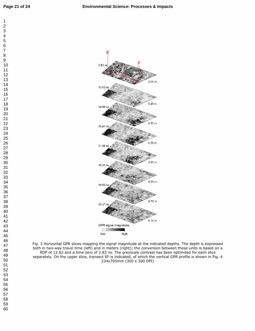
interval from 7.3 ns (or 0.19 m) to 24.9 ns (or 0.93 m), as illustrated in Fig. 3 and Fig. 4. Two features have 210

clearly added to this high signal variation. The first is the high-reflective area in the western corner of the survey 211

area, corresponding to anomaly A defined above. While the spatially exaggerated response of EMI to metallic 212

structures hampered the delineation of this anomaly, the horizontal GPR slices clearly depict its rectangular 213

boundaries (Fig. 3). The vertical profiles allow for a more precise demarcation of the anomaly's vertical extent: 214

for 0 m to 5 m along transect EF strong horizontal reflections are observed starting from the ground surface 215

down to approximately 17 ns (or 0.6 m) depth (Fig. 4). From a depth of about 13 ns (or 0.4 m) downwards on 216

Fig. 3, the horizontal slices display a second notable contrast in reflection strength at the location of anomaly B 217

in the ECa data. Vertical GPR profiles, such as the one shown in Fig. 4, demonstrate that this contrast is part of a 218

slightly dipping interface, with a larger extent than possibly expected from the horizontal slices. In Fig. 4 the 219

interface appears to extend as far as anomaly A. Yet, the lateral increase in reflection strength correlates with the 220

lower conductivity observed in the ECa maps: the lower the electrical conductivity, the weaker the GPR signal 221

attenuation and thus the stronger the reflections generated from a given soil contrast. Finally, note that the 222

locations where the ECa data indicated isolated metallic objects generally not correspond to marked anomalies in 223

the horizontal GPR slices, demonstrating that these metallic objects generally have relatively small dimensions. 224



123456789101112131415161718192021222324252627282930313233343536373839404142434445464748495051525354555657585960

9


227

3.3 Soil borings and sample analysis 228

An overview of the boring results at the six locations indicated in Fig. 2c, is given in Fig. 5. Beneath the 5 to 10 229

cm thick gravel cover, the observed soil profiles could roughly be divided into three layers (Fig. 5a). First, a 230

rather heterogeneous, brown to yellowish brown topsoil layer was seen. Particularly at location 1, the topsoil 231

contained clear anthropogenic traces such as small brick fragments and rust patches. At all six locations, the 232

bottom of the topsoil was delimited by an abrupt change to a layer with distinctly higher bulk density and 233

contrasting grey to nearly black colour. In addition to the anthropogenic traces encountered within the topsoil, 234

this layer included tiny coal fragments and a petrochemical smell was perceived at its corresponding depth at 235

locations 1 and 3. At locations 4 and 5 the contrasting layer had an abrupt lower boundary, while at the other 236

locations a gradual change into a fairly homogeneous subsoil with light grey to yellowish brown colour was 237

present. The subsoil suggested a dominant natural origin. 238

In terms of the ECp, the six locations also demonstrated a comparable vertical profile (Fig. 5b). The topsoil 239

clearly has a lower conductivity and an average jump of about 7 mS/m is observed near the upper boundary of 240

the contrasting soil layer. Together with the soil profile observations, this links the transition from the topsoil to 241

the contrasting soil layer to the interface observed in the GPR data. Consequently, the transition depths observed 242

from the soil profiles were used to estimate the average RDP of the topsoil, which, together with the earlier 243

estimated time zero, was then used to convert the GPR two-way travel time into depth in meters. Despite the 244

stringent assumption of a constant topsoil RDP, Fig. 5a and b evidence a close correspondence between the 245

estimated depth of the GPR interface and the depth of the contrasting layer as observed in the soil profiles and 246

the ECp measurements. Despite the similar within-profile ECp trend, the absolute ECp measurements differ 247

between the different locations. Whereas locations 1 and 6 show a relative constant topsoil ECp of about 11 248

mS/m, at locations 2 to 5 the topsoil ECp shows an additional dip. Below the topsoil, the between-profile 249

differences are less pronounced. 250

Soil texture analysis was only performed for locations 1, 4 and 6. With an overall average of 7.6% clay, 30.2% 251

silt and 62.2% sand, the soil texture is classified as light sandy loam (Belgian soil texture triangle), which 252

roughly confirms the data provided by the environmental assessment. As illustrated in Fig. 5c, variations in clay 253

fraction are small both within and between the profiles and do not seem to correlate with the soil layering or the 254


123456789101112131415161718192021222324252627282930313233343536373839404142434445464748495051525354555657585960

10

ECp measurements. The OM content is generally low, varying between 0.5% DM and 1.7% DM. Particularly 255

locations 2, 3 and 6 demonstrate a slightly higher OM content for the contrasting soil layer (Fig. 5c). The depth-256

weighted average of the OM content is highest at locations 1 and 6 (1.5 and 1.0% DM), although the difference 257

with locations 3 and 4 (0.98 and 0.91% DM) is very small. Each of the analyzed samples has a TPH 258

concentration far below the soil remediation threshold and target value and only for one sample (location 2, 0.5-259

0.7 m depth) the background value is exceeded (Fig. 5c). Contrary to locations 2 to 5, the TPH concentration 260

hardly exceeds the LOD at locations 1 and 6. Excepting location 3, the profiles show the highest TPH 261

concentration for the contrasting soil layer. 262

263


265

3.4 Combined interpretation of the ECa, GPR and borehole data 266

Anomaly A was clearly delineated by sharp lateral and vertical contrasts in the GPR data. The significant scatter 267

in the GPR signal in this area suggests the presence of coarse debris such as concrete rubble or bricks (e.g. 268

Boudreault et al.40). The shape and dimensions of the anomaly point to remains of a building or comparable 269

structure. The presence of metal as indicated by the ECa data further adds to this assumption given that old 270

foundations and demolition debris often contains metallic objects such as reinforcing steel bars. The assumption 271

was confirmed by surface building debris and by two soil borings encountering impenetrable material 272

immediately beneath the gravel cover (Fig. 6). A massive, probably reinforced, concrete structure and a brick 273

layer of approximately 0.5 m thickness were encountered. We note that the location of the brick layer did not 274

show the typical low-conductive signature of this material in the ECa data,40,41,42 which is likely explained by 275

nearby metallic objects dominating the EMI sensor output. An aerial photograph of the site taken in 1986 relates 276

the northeastern and southeastern edges of anomaly with a former fence (Fig. 6). In November 1985, the site 277

owner filed a request for an expansion of the existing garage. Probably the former building and its surrounding 278

aboveground infrastructure were demolished shortly after the aerial photograph had been taken and the 279

demolition debris used to level the area in preparation to the construction of the parking area. The discrete 280

metallic objects scattered over the site likely relate to the former storage of accident-involved vehicles and 281

garage activities. 282

283


123456789101112131415161718192021222324252627282930313233343536373839404142434445464748495051525354555657585960

11


285

Anomaly B is not clearly delineated by the geophysical data, suggesting that this anomaly originates from a 286

more gradual change of soil properties. In the GPR data, this anomaly appeared as a more reflective part of a 287

shallow contrasting interface occurring over a major part of the survey area. Boring investigation allowed linking 288

this interface with an abrupt transition from the topsoil to a highly disturbed layer with considerably higher bulk 289

density. The ECp measurements showed that the interface not only corresponded with a contrast in RDP, but also 290

with a change in electrical conductivity. In absence of a significant change in soil texture, the increase in 291

conductivity can likely be attributed to the increased bulk density of the contrasting soil layer, thereby suggesting 292

an effect of soil compaction (e.g. André et al.,43 Islam et al.44). Additionally, the slightly higher OM content may 293

have further contributed to a higher conductivity (e.g. Omonode and Vyn,45 Saey et al.39). The many 294

anthropogenic disturbances observed for the contrasting soil layer, including its suggested higher compaction, 295

along with its slightly higher OM content and its wide lateral extent indicated by the GPR profiles argue that its 296

upper limit represents a former living surface. Starting from this idea, the GPR reflections defining the bottom of 297

the debris fill in the western corner of the survey area probably coincide with this surface. This hypothesis is 298

further supported by the aerial photograph taken in 1986 (Fig. 6). In any case, the reorganization of the site after 299

1986 partly explains the heterogeneous appearance of the current topsoil. Through the ECa and ECp 300

measurements, the main explanation for the lateral conductivity variability could be related to a variation of the 301

properties of the current topsoil. While clay and OM content are two key 'natural' factors explaining spatial ECa 302

variations (e.g. Kühn et al.,46 Saey et al.39), in this case neither properties showed significant lateral variation. 303

Although the observed subtle variations of these properties have contributed to the resulting sensor 304

measurements, these do not fully explain the observed conductivity contrast. This suggests that the observed 305

lateral contrast may also have predominantly anthropogenic cause. Here, TPH concentration is the only property 306

that showed a distinct difference between the boring locations as the LOD was only clearly exceeded at the 307

locations within the low conductive zone. A decrease in electrical conductivity of the upper vadose zone due to 308

the presence of a hydrocarbon contamination has been reported before (e.g. DeRyck et al.47) and has been 309

suggested to relate to vapor effects.22 A negative correlation between TPH concentration and electrical 310

conductivity generally relies on the assumption that the effect of biodegradation is negligible. Even so, 311

considering previous research (e.g. Daniels et al.,14 Sauck,20 Carcione et al.11), it is questionable whether TPH 312

concentrations lower than 50 mg/kg DM (equivalent to a hydrocarbon saturation lower than about 0.0001) are 313


123456789101112131415161718192021222324252627282930313233343536373839404142434445464748495051525354555657585960

12

able to cause a conductivity decrease of several millisiemens per meter. In this respect, it is more plausible that 314

the slightly elevated TPH concentration is a proxy for a more complex physico-chemical soil disturbance that 315

could not be fully defined by the limited number of properties that were analyzed on the boring samples. 316

Regarding the within-profile coincidence of the highest TPH concentration and the highest conductivity, we 317

propose two hypotheses. The first assumes that each of the observed hydrocarbon concentrations, irrespective of 318

the depth at which they are observed, corresponds to a relatively fresh and, hence, non-degraded contamination. 319

In this case, the higher OM content and soil bulk density have dominated the GPR and ECp measurements 320

beneath the topsoil, but may have caused a higher retention of petroleum hydrocarbons in the contrasting soil 321

layer.48,49 The second hypothesis assumes that the hydrocarbon concentrations observed in the contrasting soil 322

layer relate to an older contamination event than those observed in the topsoil and that, with time, biodegradation 323

processes have added to an increase in electrical conductivity of this layer. Which of the two hypotheses is true 324

cannot be determined with absolute certainty because no direct information on the occurrence of biodegradation 325

was available. Yet, for locations 1, 2, 4 and 5, the composition of the hydrocarbon mixture showed smaller 326

fractions of hydrocarbons in the C10 to C20 range in the contrasting soil layer as compared to the topsoil. 327

Considering that the biodegradable fraction of petroleum hydrocarbons mainly consists in C12-C20 328

hydrocarbons (e.g. Minai-Tehrani et al.50), this may be an indication in favour of the second hypothesis. The 329

contamination of the contrasting layer possibly even dates from before the site was reorganized at the end of the 330

1980s and in that case may also have a different lateral extent than the topsoil contamination. 331

6 Conclusions 332

Our case study demonstrated the use of combining multi-receiver EMI and stepped-frequency GPR to pinpoint 333

locations of anthropogenic soil disturbances, particularly of those having affected physical soil properties. The 334

identification of a soil layer with considerably higher bulk density exemplified the methodology's potential to 335

improve insight in the upper soil stratification, which in turn could aid the understanding of the local soil-336

forming processes. Furthermore, the sharp delineation of the building remains illustrated the high accuracy that 337

can be achieved in spatially characterizing structures of technogenic material. Since such physical soil contrasts 338

locally can have a strong influence on the distribution and dispersion of contaminants, they can represent 339

important targets in the investigation of contaminated urban soils. The demonstrated correspondence between a 340

zone of remarkably lower electrical conductivity and slightly elevated TPH concentrations suggests the potential 341

for the sensor combination to detect specific chemical soil disturbances too. However, further investigation 342


123456789101112131415161718192021222324252627282930313233343536373839404142434445464748495051525354555657585960

13

should aim at the expansion of the presented methodology to other conditions of contamination with petroleum 343

hydrocarbons, including a wider range of concentrations and biodegradation stages. 344

This case study proves the advantage of the sensors to rapidly screen urban soils for geophysical anomalies, but 345

also indicates that interpretation of these anomalies in terms of anthropogenic disturbances might not always be 346

straightforward. This can be complicated further when metallic objects are prevalent in the studied urban 347

environment. Specifically EMI is very sensitive to such local high conductors causing the geophysical signature 348

of the soil material directly surrounding them to be compromised. Yet, the guaranteed detection of metallic 349

objects may be an advantage in case they represent major targets in the site's investigation.38 In any case, the 350

detailed 3D soil information provided by the sensor combination offers a sound guide for the initial sampling 351

design of invasive investigation. So-designed boring investigation can serve as ground truth and can aid in 352

selecting the relevant geophysical anomalies for more in-depth investigation. Generally, we conclude that the 353

proposed methodology is particularly valuable in an exploratory phase of urban soil assessment, to direct future 354

(invasive) investigation and to support the intra- and extrapolation of information derived therefrom. 355

Acknowledgements 356

The authors would like to thank Gert Moerenhout and Sven Van Daele from the Soil Remediation Fund for 357

Petrol Stations (BOFAS) for introducing this case study and for providing all the earlier collected site 358

information. We also thank the owner-occupiers for their kind hospitality during our visits and Valentijn Van 359

Parys for his help with the EMI and GPR surveys. 360

361

References 362

1 C. R. De Kimpe and J. L. Morel, Soil Sci., 2000, 165(1), 31-40. 363

2 A. Lehmann and K. Stahr, J. Soils and Sediments, 2007, 7(4), 247-260. 364

3 H. Meuser, in Contaminated Urban Soils. Environmental pollution, 18. ed. B. J. Alloway and J. T. Trevors, 365

Springer Science, New York, 2010, ch. 2, pp. 5-27 . 366

4 S. Norra and D. Stüben, J. Soils and Sediments, 2003, 3(4), 230-233. 367

5 J. D. Redman, in Ground Penetrating Radar: Theory and Applications ed. H. M. Jol, Elsevier Science, 368

Amsterdam, 2009, ch. 8, pp. 247-269. 369


123456789101112131415161718192021222324252627282930313233343536373839404142434445464748495051525354555657585960

14

6 V. I. Adamchuk, J. W. Hummel, M. T. Morgan and S. K. Upadhyaya, Comput. Electron. Agric., 2004, 44, 71-370

91. 371

7 D. L. Corwin and S. M. Lesch, Comput. Electron. Agric., 2005, 46, 11-43. 372

8 L. Verdonck, D. Simpson, W. M. Cornelis, A. Plyson, J. Bourgeois, R. Docter and M. Van Meirvenne, 373

Archaeological Prospection, 2009, 16, 193-202. 374

9 P. De Smedt, M. Van Meirvenne, D. Herremans, J. De Reu, T. Saey, E. Meerschman, P. Crombé, and W. De 375

Clercq, Sci. Rep., 2013, 3(1517), 1-5. 376

10 T. Saey, M. Van Meirvenne, P. De Smedt, W. Neubauer, I. Trinks, G. Verhoeven, and S. Seren, Eur. J. Soil 377

Sci., 2013, 64, 716-727. 378

11 J. M. Carcione, G. Seriani, and D. Gei, J. Appl. Geophys., 2003, 52(4), 177-191. 379

12 N. J. Cassidy, J. Contam. Hydrol., 2007, 94, 49-75. 380

13 M. L. Brewster, A. P. Annan, J. P. Greenhouse, B. H. Kueper, G. R. Olhoeft, J. D. Redman and K. A. Sander, 381

Ground Water, 1995, 33(6), 977-987. 382

14 J. J. Daniels, R. Roberts and M. Vendl, J. Appl. Geophys., 1995, 33(1-3), 195-207. 383

15 J. C. Santamarina and M. Fam, J. Environ. Eng. Geophys., 1997, 2, 37-52. 384

16 S. Jin, P. Fallgren, J. Cooper, J. Morris and M. Urynowicz, J. Environ. Sci. Health, Part A: Toxic/Hazard. 385

Subst. Environ. Eng., 2008, 43(6), 584-588. 386

17 H. P. Martinelli, F. E. Robledo, A. M. Osella and M. de la Vega, J. Appl. Geophys., 2012, 77, 21-29. 387

18 E. A. Atekwana, W. A. Sauck and D. D. Werkema, J. Appl. Geophys., 2000, 44(2-3), 167-180. 388

19 E. D. Guy, J. J. Daniels, J. Holt and S. J. Radzevicius, J. Environ. Eng. Geophys., 2000, 5(2), 11-19. 389

20 M. de la Vega, A. Osella and E. Lascano, J. Appl. Geophys., 2003, 54, 97-109. 390

21 W. A. Sauck, J. Appl. Geophys., 2000, 44, 151-165. 391

22 D. D. Werkema Jr., E. A. Atekwana, A. L. Endres, W. A. Sauck and D. P. Cassidy, Geophys. Res. Lett., 2003, 392

30(12), 1647. 393

23 E. A. Atekwana and E. A. Atekwana, Surv. Geophys., 2010, 31, 247-283. 394

24 E. Auken, L. Pellerin, N. B. Christensen and K. Sørensen, Geophys., 2006, 71(5), G249-G260. 395


123456789101112131415161718192021222324252627282930313233343536373839404142434445464748495051525354555657585960

15

25 VLAREBO, Flemish Soil Remediation Decree ratified by the Flemish Government on 14 December 2007, 396

Belgisch Staatsblad, April 22, 2008. 397

26 G. V. Keller and F. C. Frischknecht, Electrical methods in geophysical prospecting, Pergamon Press, Oxford, 398

1966. 399

27 J. D. McNeill, Electromagnetic terrain conductivity measurements at low induction number, Technical Note 400

TN-6, Geonics Limited, Ontario, 1980. 401

28 T. Saey, D. Simpson, L. Cockx and M. Van Meirvenne, Soil Sci. Soc. Am. J., 2009, 73(1), 7-12. 402

29 D. Simpson, A. Lehouck, M. Van Meirvenne, J. Bourgeois, E. Thoen and J. Vervloet, Geoarchaeol. Int. J., 403

2008, 23(2), 305-319. 404

30 K. R. Sheets and J. M. Hendrickx, Water Resour. Res., 1995, 31(10), 2401-2409. 405

31 P. Goovaerts, Geostatistics for Natural Resource Evaluation, Oxford University Press, New York, USA, 406

1997. 407

32 T. Saey, M. Van Meirvenne, M. Dewilde, F. Wyffels, P. De Smedt, E. Meerschman, M. M. Islam, F. Meeuws 408

and L. Cockx, Near Surf. Geophys., 2011, 9, 309-317. 409

33 S. Koppenjan, in Ground Penetrating Radar: Theory and Applications, ed. H. M. Jol, Elsevier Science, 410

Amsterdam, 2009, ch. 3, pp. 73-97. 411

34 N. J. Cassidy, in Ground Penetrating Radar: Theory and Applications, ed. H. M. Jol, Elsevier Science, 412

Amsterdam, 2009, ch. 5, pp. 141-176. 413

35 J. D. Rhoades and J. van Schilfgaarde, Soil Sci. Soc. Am. J., 1976, 40(5), 647-651. 414

36 ISO 11277, Soil quality - Determination of particle size distribution in mineral soil material - Method by 415

sieving and sedimentation, 2009. 416

37 ISO/DIS 9377-4, Water Quality - Determination of hydrocarbon oil index - Part 4: Method using solvent 417

extraction and gas chromatography, 1999. 418

38 E. Van De Vijver, M. Van Meirvenne, T. Saey, S. Delefortrie, P. De Smedt, J. De Pue and P. Seuntjens, Eur. 419

J. Soil Sci., 2015, DOI: 10.1111/ejss.12229. 420

39 T. Saey, M. Van Meirvenne, H. Vermeesch, N. Ameloot and L. Cockx, Geoderma, 2009, 150, 389-395. 421

40 J. P. Boudreault, J. S. Dubé, M. Chouteau, T. Winiarski and É. Hardy, Eng. Geol., 2010, 116, 196-206. 422


123456789101112131415161718192021222324252627282930313233343536373839404142434445464748495051525354555657585960

16

41 D. Simpson, A. Lehouck, M. Van Meirvenne, J. Bourgeois, E. Thoen and J. Vervloet, Geoarchaeol. Int. J., 423

2008, 23(2), 305-319. 424

42 D. Simpson, M. Van Meirvenne, T. Saey, H. Vermeersch, J. Bourgeois, A. Lehouck, L. Cockx and U. W. A. 425

Vitharana, Archaeol. Prospect., 2009, 16, 91-102. 426

43 F. André, C. van Leeuwen, S. Saussez, R. Van Durmen, P. Bogaert, D. Moghadas, L. de Rességuier, B. 427

Delvaux, H. Vereecken and S. Lambot, J. Appl. Geophys., 2012, 78, 113-122. 428

44 M. M. Islam, E. Meerschman, T. Saey, P. De Smedt, E. Van De Vijver, S. Delefortrie and M. Van 429

Meirvenne, Soil Sci. Soc. Am. J., 2014, 78, 579-588. 430

45 R. A. Omonode and T. J. Vyn, Soil Sci., 2006, 171(3), 223-238. 431

46 J. Kühn, A. Brenning, M. Wehrhan, S. Koszinski and M. Sommer, Precision Agric., 2009, 10(6), 490-507. 432

47 S. M. DeRyck, J. D. Redman and A. P. Annan, in Proceedings of the symposium on the application of 433

geophysics to engineering and environmental problems (SAGEEP), Environmental and Engineering Geophysical 434

Society, Wheat Ridge, CO, United States, 1993, pp. 5-19. 435

48 P. Fine, E. R. Graber and B. Yaron, Soil Technol., 1997, 10, 133-153. 436

49 M. Yang, Y. S. Yang, X. Du, Y. Cao and Y. Lei, Water, Air, Soil Pollut., 2013, 224(3), 1439. 437

50 D. Minai-Tehrani, P. Rohanifar and S. Azami, Int. J. Environ. Sci. Technol., 2015, 12, 1253-1260. 438

439


123456789101112131415161718192021222324252627282930313233343536373839404142434445464748495051525354555657585960

17

Figure captions 440

Fig. 1 Outline map of the study site with indication of the invasive investigation locations of the environmental 441

assessment carried out between 2008 and 2012 and the consequent delineation of the soil contamination with 442

petroleum hydrocarbons according to the TPH concentration thresholds provided by the Flemish soil 443

remediation legislation (background value 50 mg/kg DM, target value 300 mg/kg DM and soil remediation 444

threshold 750 mg/kg DM) (left); aerial photograph of the study site in 2012 which still shows stored vehicles at 445

the parking area (right) 446

Fig. 2 a ECa maps for the four coil configurations of the EMI sensor; measurement values outside the colour 447

scale were assigned the same colour as the scale limits; b FEMP map; c 1HCP ECa map with indication of 448

anomalies A and B, and the locations selected for additional boring investigation of anomaly B 449

Fig. 3 Horizontal GPR slices mapping the signal magnitude at the indicated depths. The depth is expressed both 450

in two-way travel time (left) and in meters (right); the conversion between these units is based on a RDP of 451

12.62 and a time zero of 2.83 ns. The greyscale contrast has been optimised for each slice separately. On the 452

upper slice, transect EF is indicated, of which the vertical GPR profile is shown in Fig. 4 453

Fig. 4 Vertical GPR profile showing the real part of the GPR response in function of depth along transect EF, 454

without (top) and with (bottom) indication of the contrasting interface 455

Fig. 5 a Schematic representation of the soil profiles at the six locations indicated in Fig. 2c showing four 456

different soil layers in the upper 1.75 m of soil, with an illustration of the actual observation for 10-60 cm depth 457

at location 3; b ECp (top axis) in function of depth ("�"; the vertical lines indicate the depth intervals for which 458

the measurements are representative) and the local GPR signal magnitude (bottom axis) in function of depth 459

divided by the local maximum magnitude (relative); the depth is expressed both in meters (left axis) and in two-460

way travel time (right axis) c clay fraction (upper top axis, "֠"), OM content (lower top axis, "�") and TPH 461

concentration (bottom axis, "�") in function of depth; the vertical dashed line indicates the LOD (20 mg/kg 462

DM) for the TPH concentration; TPH analysis results below the LOD are represented by a concentration of 10 463

mg/kg DM 464

Fig. 6 Field verification of the interpretation of anomaly A (Fig. 2c) as fill with demolition debris (left) and 465

aerial photograph of the site taken in 1986 showing the former building and aboveground infrastructure near the 466

location of anomaly A (Source: Department of Archaeology, Ghent University, J. Semey) (right) 467


123456789101112131415161718192021222324252627282930313233343536373839404142434445464748495051525354555657585960

Fig. 1 Outline map of the study site with indication of the invasive investigation locations of the environmental assessment carried out between 2008 and 2012 and the consequent delineation of the soil contamination with petroleum hydrocarbons according to the TPH concentration thresholds provided by the

Flemish soil remediation legislation (background value 50 mg/kg DM, target value 300 mg/kg DM and soil remediation threshold 750 mg/kg DM) (left); aerial photograph of the study site in 2012 which still shows

stored vehicles at the parking area (right) 125x90mm (300 x 300 DPI)


123456789101112131415161718192021222324252627282930313233343536373839404142434445464748495051525354555657585960

282x537mm (300 x 300 DPI)


123456789101112131415161718192021222324252627282930313233343536373839404142434445464748495051525354555657585960

Fig. 3 Horizontal GPR slices mapping the signal magnitude at the indicated depths. The depth is expressed both in two-way travel time (left) and in meters (right); the conversion between these units is based on a

RDP of 12.62 and a time zero of 2.83 ns. The greyscale contrast has been optimised for each slice

separately. On the upper slice, transect EF is indicated, of which the vertical GPR profile is shown in Fig. 4 234x705mm (300 x 300 DPI)


123456789101112131415161718192021222324252627282930313233343536373839404142434445464748495051525354555657585960

Fig. 4 Vertical GPR profile showing the real part of the GPR response in function of depth along transect EF, without (top) and with (bottom) indication of the contrasting interface

110x70mm (300 x 300 DPI)


123456789101112131415161718192021222324252627282930313233343536373839404142434445464748495051525354555657585960

Fig. 5 a Schematic representation of the soil profiles at the six locations indicated in Fig. 2c showing four different soil layers in the upper 1.75 m of soil, with an illustration of the actual observation for 10-60 cm depth at location 3; b ECp (top axis) in function of depth ("0"; the vertical lines indicate the depth intervals

for which the measurements are representative) and the local GPR signal magnitude (bottom axis) in function of depth divided by the local maximum magnitude (relative); the depth is expressed both in meters (left axis) and in two-way travel time (right axis) c clay fraction (upper top axis, "%"), OM content (lower top

axis, ")") and TPH concentration (bottom axis, ">") in function of depth; the vertical dashed line indicates the

LOD (20 mg/kg DM) for the TPH concentration; TPH analysis results below the LOD are represented by a concentration of 10 mg/kg DM 234x331mm (300 x 300 DPI)


123456789101112131415161718192021222324252627282930313233343536373839404142434445464748495051525354555657585960

88x45mm (300 x 300 DPI)


123456789101112131415161718192021222324252627282930313233343536373839404142434445464748495051525354555657585960

Date post:	21-Nov-2021
Category:	Documents
Upload:	others
View:	1 times
Download:	0 times

Urban soil exploration through multi-receiver ...

Documents