General rights Copyright and moral rights for the publications made accessible in the public portal are retained by the authors and/or other copyright owners and it is a condition of accessing publications that users recognise and abide by the legal requirements associated with these rights. Users may download and print one copy of any publication from the public portal for the purpose of private study or research. You may not further distribute the material or use it for any profit-making activity or commercial gain You may freely distribute the URL identifying the publication in the public portal If you believe that this document breaches copyright please contact us providing details, and we will remove access to the work immediately and investigate your claim. Downloaded from orbit.dtu.dk on: Nov 30, 2021 Utilization of on-line corrosion monitoring in the flue gas cleaning system Montgomery, Melanie; Nielsen, Lars V. ; Petersen, Michael B. Published in: Proceedings of NACE Corrosion 2015 Publication date: 2015 Document Version Peer reviewed version Link back to DTU Orbit Citation (APA): Montgomery, M., Nielsen, L. V., & Petersen, M. B. (2015). Utilization of on-line corrosion monitoring in the flue gas cleaning system. In Proceedings of NACE Corrosion 2015 [5550] NACE International.
Transcript
General rights Copyright and moral rights for the publications made accessible in the public portal are retained by the authors and/or other copyright owners and it is a condition of accessing publications that users recognise and abide by the legal requirements associated with these rights.
Users may download and print one copy of any publication from the public portal for the purpose of private study or research.
You may not further distribute the material or use it for any profit-making activity or commercial gain
You may freely distribute the URL identifying the publication in the public portal If you believe that this document breaches copyright please contact us providing details, and we will remove access to the work immediately and investigate your claim.
Downloaded from orbit.dtu.dk on: Nov 30, 2021
Utilization of on-line corrosion monitoring in the flue gas cleaning system
Montgomery, Melanie; Nielsen, Lars V. ; Petersen, Michael B.
Published in:Proceedings of NACE Corrosion 2015
Publication date:2015
Document VersionPeer reviewed version
Link back to DTU Orbit
Citation (APA):Montgomery, M., Nielsen, L. V., & Petersen, M. B. (2015). Utilization of on-line corrosion monitoring in the fluegas cleaning system. In Proceedings of NACE Corrosion 2015 [5550] NACE International.
Utilization of on-line corrosion monitoring in the flue gas cleaning system
Melanie Montgomery COWI AS / Technical University of Denmark
Parallelvej 2, 2800 Kgs Lyngby,
Denmark
Lars V. Nielsen and Michael B. Petersen Metricorr ApS
Produktionsvej 2 2600 Glostrup
Denmark
ABSTRACT
Amager unit 1 is a 350 MWth multifuel suspension-fired plant commissioned in 2009 which fires biomass. Increasing corrosion problems in the flue gas cleaning system have been observed since 2011 in both the gas-gas preheater and the booster fan and booster fan duct. A root cause analysis concluded that corrosion occurs due to corrosion products/deposit formed during operation; however it was unclear whether the majority of corrosion occurred during operation or downtime. In both cases the chlorine content in the flue gas results in the presence of chlorine species such as HCl, KCl or chlorine containing corrosion products. Without knowing when corrosion occurs, it is difficult to take reasonable measures to reduce corrosion. In order to gain an improved understanding of the corrosion problem, an on-line corrosion measurement system was established before the booster fan. The corrosion rates measured with respect to time were correlated to plant data such as load, temperature, gas composition, water content as well as change in the fuel used. From these results it is clear that many shutdowns/start-ups influence corrosion and therefore cause decreased lifetime of components and increased maintenance. A fuel change from a mix of straw and wood pellets to only wood pellets has also decreased corrosion.
The combustion of biomass instead of coal results in material challenges due to the chlorine content of the fuel. In the past two decades, much research has been conducted in this area due to the formation of alkali chlorides during combustion resulting in high temperature corrosion.1 Thus when the multifuel suspension-fired plant Amager 1 was built in Denmark, both the material choice and outlet temperature in the superheaters were in accordance with the most recent experiences.2 However the potential corrosion problems in the cold end were not given the same rigorous assessment. Initially the plant was termed a multifuel firing plant where biomass would be co-fired with fossil fuels and for short periods of time burnt alone. Therefore it was built with a desulphurization plant which was to be used when fossil fuels were fired. However when the plant was commissioned, it was decided that it should be 100% bio-fuelled (both straw and wood pellets). A fossil-fuelled plant would have different flue gas composition and therefore different corrosion problems, both in the superheaters but also in the tail end. In recent
years examples of biomass plants with tail-end corrosion problems related to the chlorine content in the flue gas have been reported in Sweden3,4, Denmark5,6, Germany7 and Canada8. This paper summarizes the problems observed at Amager power plant, and describes implementation and results of on-line measurements.
DESCRIPTION OF AMAGER POWER PLANT
Amager unit 1 was first operational in 1971 as a coal-fired plant. It was re-commissioned in 2009 after an extensive renovation to a 350 MWth multifuel suspension-fired plant. Since then the primary fuel has been biomass (straw and wood pellets). The flue gas analysis from firing 100% wood as well as 100% straw pellets measured after the electrostatic precipitator is given in Table 1.
Table 1 Flue gas composition measured after the electrostatic precipitator (*below detection limits).
H2O CO2 CO N2O NO NO2 SO2 NH3 HCl HF CH4 NOx Oxygen
The fuel utilized has been 400,000 tons/year biomass. Up until 2014, 25% of the fuel has been straw pellets, however since December 2013, only wood pellets have been used. Since the two fuels are mixed, it has been difficult to know the ratio of straw pellets to wood pellets fired at any point in time. This information would have been advantageous for the assessment of corrosion potential as the HCl content from the flue gas for wood pellets is an order of magnitude lower than straw pellets. Since the flue gas goes through the FGD (flue gas desulphurization) plant, the levels of HCl and SO2 will be reduced considerably since both HCl and KCl are highly water soluble.
Figure 1: Schematic of flue gas cleaning system at Amager 1.
Stack
Electrofilter
Booster Fan
Desulphurisation
DeNOx Bypass
Gas-gas heat exchanger
Waste water treatment plant
Induced draft fan
Corrosion sensors placed in duct between booster fan and gas-gas heater
FGD AMV 1
Figure 1 is a schematic diagram of the flue gas cleaning system (FGCS). The GAFO (gas/gas heat exchanger referred to in this paper as GAFO = “gasforvarmer”) is a rotating regenerative heat exchanger on a counter flow principle. Heat transfer elements in the GAFO are placed as a matrix in an open rotor which transfers heat from one gas side to the other whilst slowly rotating. Both the rotor and the heat transfer elements are fabricated in a weathering steel A242 with tradename CORTEN A1. However in the lower part of the GAFO, these elements are further protected by an enamel coating. The inlet gas side is fabricated in UNS S31254 (254 SMO2) and the outlet “clean” gas side in A242 steel. Flue gas (~51°C) from the FGD plant is heated to approx. 300°C and led through the deNOx plant. Then the “clean” gas returns to the GAFO heat exchanger where it is cooled to approx. 85ºC and flows via the booster fan to the stack. The ducts after the GAFO are carbon steel, as is the booster fan.
CORROSION OBSERVATIONS
Increasing corrosion problems in the flue gas cleaning system (FGCS) had been observed since 2011 in the GAFO, where A242 steel corroded by 2 mm in 2 years. The AISI 316 bolts holding the sealing strips suffered from stress corrosion cracking leading to detachment of the UNS N10276 (Hastelloy C-2763) radial sealing strips.9 It was clear that the extensive corrosion was localized to the lower part of the GAFO –predominantly in the inner part and at the periphery. Investigations of the corrosion product showed a layered oxide where the highest chlorine concentration was detected close to the metal surface. Therefore the presence of chlorine had not given the optimal conditions for formation of a protective layer. Corrosion products removed from the lower part of the GAFO were mostly iron oxide (goethite). However at the inner surface attached to the metal, chlorine was present and akaganeite was detected. Close to the flue gas-oxide interface, more sulfur rich products were found together with iron, i.e. iron sulfate. Fine particles of potassium chloride were also observed. Varying degrees of corrosion were observed where the area closest to the rotor and at the periphery were the worst (Figure 2a). With the temperature of the GAFO rotor changing from 51ºC to 85ºC, some corrosion would be expected. However in some areas where the flue gas was warmer (approx 285°C in normal operation), corrosion was also observed (Figure 2b).
a) Outlet to GAFO close to axel b) Above the GAFO on inlet side
Figure 2: Different types of corrosion observed in GAFO
Corrosion was also observed in the booster fan and duct where the temperature was ~85⁰C. Various forms of corrosion including pitting of the duct and corrosion/erosion patterns of the booster blades were also observed. Erosion could be due to water droplets in the flue gas stream entrained from the FGD, however also spalled rust from the GAFO would lead to erosion.
1 CORTEN is a tradename from US Steel. 2 254SMO is tradename from Avesta. 3 Hastelloy C-276 is a tradename from Haynes
The following summarizes the corrosion observed in FGCS:
Corrosion of A242 in the lower part of the GAFO, also on the enameled elements.
Stress corrosion cracking of UNS S31600 bolts (replaced with UNS N10276 bolts)
Pitting corrosion in the duct near the booster fan
Downtime corrosion: in hotter locations in GAFO, booster blades, booster canal
Erosion, corrosion and pitting of the booster blades
Although the outlet temperature for the GAFO is 85⁰C the inlet from the desulphurization plant is 51ºC. It takes approx. 75 seconds for the GAFO to make a full rotation, where the temperature of the lower part cycles from 51°C to 85°C. Thus the majority of time, the lower part of the GAFO will be below 85°C. In comparison to carbon steel, weathering steel should be able to form a more protective layer with the changing wet-dry cycles. This principle has been successful for gas preheaters where coal has been the fuel. However A242 does not form such a protective coating if chlorine species such as HCl is present. The condensation of HCl from the flue gas is dependent on the moisture content and the concentration of HCl in the gas phase10. Thus condensation of HCl when firing with straw pellets based on water content in flue gas will be 51-52⁰C which is slightly higher than the water dewpoint. The lower part of the GAFO will be within this temperature window for HCl dewpoint condensation every 75 seconds. In other parts of the FGCS, such as warmer parts of the GAFO and in the duct after the GAFO, the temperature is higher, and the flue gas goes through the dewpoint temperature only on start-up and shutdown. There were signs of both downtime corrosion in this area but also corrosion during operation. Thus the various corrosion observations on different components on different occasions made it difficult to pinpoint the precise cause of corrosion.
IMPLEMENTATION OF ON-LINE MEASUREMENTS
There are many different corrosion mechanisms and in order to understand individual corrosion contributions, it was decided to implement on-line measurements. It was hoped that this would reveal when the majority of corrosion was occurring so that it could be combatted. The usual way to monitor low temperature corrosion is with standard electrochemical measuring tools such as polarization and impedance, however since the corroding structures are not immersed in a liquid phase and corrosion occurs due to a surface film of water (similar to atmospheric corrosion) such techniques are not applicable. In addition these techniques will not measure material loss from erosion. The alternative is to use a corrosion sensor which is exposed for 3-4 weeks and then assessed by weight loss measurements such that the corrosion rates over a period of time can be measured. Information with respect to changing operation parameters in the plant are however not available with this method. Thus an ER (electrical resistance) on-line corrosion measurement system11 was installed before the booster fan, and ER sensors measured thickness reduction every 30 minutes such that corrosion events could be correlated to the operation data of the plant. Description of Metricorr4 ER Sensor
This ER technique is used extensively in the oil and gas industry, but has not been used in fluctuating temperatures and flue gas compositions common to power plants. However there have been tests to validate the temperature stability of the sensors in an interval from 50⁰C to room temperature.12 The online corrosion sensors measures metal loss by comparing the electrical resistance of two identical elements built into the ER (Electrical Resistance) sensor. One element is exposed to the environment
4 Metricorr is a Tradename
and diminishes in thickness due to corrosion. The resistance of the exposed element changes with thickness and temperature.
.).(
W
LTR
R= resistance, W= thickness, L= length, W= width, ρ(T) resistance of element material. A second element, a reference element is shielded from the hostile environment. The resistance of the reference element changes with temperature and is used to compensate temperature fluctuations. Thus the exposed elements corrosion rate (as loss in metal thickness) with respect to time can be quantified. Corrosion rate can be monitored in downtime and during exposure, and with changes of other operating parameters in the plant (such as fuel, humidity, temperature). Four corrosion sensors were installed as shown in Figure 3. Sensors were fabricated in mild steel with different thickness (3 at 500 µm and 1 at 1000 µm as the rate of corrosion was not known) and at different angles to the flue gas flow (30°, 90° and parallel to the duct wall) in the location shown in Figure 1. Angled probes were chosen to try to measure the erosion contribution experienced by the booster blades which are positioned in the middle of the duct.
a) In the plant b) Sectioned on white dotted line
Figure 3: Photographs of ER sensor.
The sensors were installed during the summer overhaul 2013 and data has been collected for 11 months. The sensor location from the top is P1, P2, P4 and P3. It was clear that there are more deposit/corrosion products on the sensor angled perpendicular to the flue gas. The 500 µm sensors were removed in July 2014 and subjected to destructive analysis to verify the reliability of the measurements. They were cross-sectioned (Figure 3b) and measured to compare the thickness measurements with the ER measurements.
RESULTS
Data was collected by a modem and sent daily to Amager power plants DCS (distributed control system). The ER data could then be correlated with data from the plant to reveal which operation conditions trigger a corrosion incidence. To check the validity of the measurements, three of the sensors were removed during the summer stop in 2014 and the thickness of the sensor elements was measured with microscopy. In addition, the corrosion morphology could also be assessed.
On-line measurements correlated with operation data
The 1000 µm sensor showed similar trends to the 500 µm, so in this paper, the information from the 500 µm sensor will be used. Since similar trends were observed, the 500 µm sensors were replaced with 1000 µm sensors to give a longer lifetime. Figure 4 compares the data for the 500 µm sensors and it can clearly be observed that the sensors which are not parallel to the duct wall have a tendency to a higher corrosion rate even at the beginning of the exposures in August 2013, where the 90º angled sensor had the higher thickness loss. Visual observation showed there is more deposit/corrosion product on the sensors not parallel to the wall such that deposit amount decreases as follows 90º>30º>0º. Different plant data was correlated to the sensor data. The main parameters are temperature and water content in the flue gas, however other characteristics such as plant load, flue gas flow, SO₂, NOX O₂, soot blowers, etc. were correlated. The water content measurement was not close to the sensor but from the stack, so although it is a useable measurement when the plant is in operation, this is not the case during shutdown or bypass operation. There is not a gradual metal loss but there are events which precipitate thickness reduction, and these are indicated on Figure 4.
Figure 4: Comparison of 500 µm sensors from July 2013-July 2014.
It was clear that in 2013, these events coincided with shutdown/start-up episodes as shown in Figure 5. When water content in the flue gas drops, this indicates that the plant has been shut down. In some cases the temperature in the FGCS is kept warm, however if access to the FGCS is required, this part of the plant is cooled rapidly. The start-up of the plant is marked with arrows A, B, C, D, E and F on Figure 4. The arrow F, also corresponds to a startup, however there is no increased corrosion. Event A was when the plant was started up on 31st July 2013 after the corrosion sensors were installed. The corrosion sensors were newly prepared and without visible deposit. Figure 6 illustrates how corrosion began during start-up where the flue gas flow started, and the corrosion increased first during start up, probably to form the initial oxide layer (3-4µm), but then continued for a short time after start-up. The flow varied during start-up, but apart from the initial start-up, this cannot be linked with the thickness decrease in the sensors. There were also spikes from SO₂ and NO/NOX during start-up.
No data was collected for Event B but it seems to indicate the same profile as Event A: a high initial corrosion rate followed by a lower corrosion rate which after some time was negligible.
Figure 5: Corrosion profile correlated to temperature and water/oxygen content in the stack.
Figure 6: Event A – Corrosion profile correlated to start-up conditions
For Event C, an increase in corrosion as the plant is shut down was observed followed by a gradual corrosion rate on start-up which lasted almost a month.
0
50
100
150
200
250
300
350
400
450
500
0
20
40
60
80
100
120
140
160
Probe thickn
ess µm
Water in
vol%
/ Tem
p in
°C
Water in stack vol% Temp adjacent probe °C Parallel P1
Flow booster fan kg/s SO₂ in stack mg/Nm³ Water in stack vol%
Temp adjacent probe °C Parallel P1 30° to duct wall P2
90 ° to duct wall P3
Figure 7: Event C - Short shutdown where GAFO temperature is decreased.
It is evident that the 90º sensor and 30º sensors incurred more corrosion compared to the sensor parallel the duct wall and that this corrosion or erosion occurred whilst the plant was in operation. The only operation condition which could correlate with this event was the variable flow caused by variable load (Figure 8). A higher load means that there is greater flow of flue gas, but also more movement of deposit/water droplets through the system. Reasons for higher corrosion or erosion due to changing load are difficult to explain.
Figure 8: Corrosion profile with respect to load.
280
300
320
340
360
380
400
420
440
460
0
50
100
150
200
250
Probe thickn
ess µm
Operation param
eters
Flow booster fan kg/s Water in stack vol% Temp adjacent probe °C
Parallel P1 30° to duct wall P2 90 ° to duct wall P3
0
50
100
150
200
250
300
350
400
450
500
0
20
40
60
80
100
120
140
160
180
200
Probe thickn
ess µm
Load
%
Load % µm Thickness (µm) Parallel P1
µm Thickness (µm) 30° to duct wall P2 µm Thickness (µm) 90 ° to duct wall P3
Event D consists of two sub events (D1 and D2) which closely follow one another (Figure 9). The plant was shut down around the 2nd November 2013, and the GAFO was kept warm. Only marginal corrosion was observed during shutdown although there was a short temperature spike in the GAFO (probably someone opened a manhole). When the plant came back into operation, the corrosion started.
Figure 9: Event D - Corrosion profile with respect to temperature and water content.
Figure 10: Event E - Corrosion profile with respect to temperature and water content.
350
360
370
380
390
400
410
420
430
440
450
0
50
100
150
200
250
Probe thickn
ess µm
Water vol% / Temp °C
Water in stack vol% Temp adjacent probe °C Parallel P1
30° to duct wall P2 90 ° to duct wall P3
200
250
300
350
400
0
20
40
60
80
100
120
140
160
Probe thickn
ess µm
Water content % / Tem
perature°C
EVENT EWater in stack vol% Temp adjacent probe °C Parallel P1
30° to duct wall P2 90 ° to duct wall P3
Again there was a gradual corrosion rate and it had probably not yet reached its full extent before the next shutdown occurred a few days later. Start-up again precipitated corrosion and continued as a gradual corrosion rate over the next two weeks. There was no sharp increase in corrosion before the gradual corrosion as seen in Event A.
From December 2013, only wood pellets were fired. The corrosion profile of Event E showed a slightly higher corrosion rate after start-up which then continued with a slower corrosion rate for about two months. During February, the corrosion rate of the 90° sensor increased slightly more than the others, and slightly higher water content in the flue gas was measured. Event E had the largest metal loss although it was a period when only wood pellets were used. The final event F is somewhat a non-event and therefore the most interesting (Figure 11). The plant was shut down and started up with negligible effect on corrosion.
Figure 11: Event F - Corrosion profile with respect to temperature and water content.
Analysis of sensors
The exposed corroded element of the sensors was cross-sectioned as shown in Figure 3b. The reference element behind the exposed element of the sensor was measured to 481 µm (±2 µm). For the on-line measurements, the reference thickness was set to either 500 µm or 1000 µm and the corrosion was monitored relative to this set reference. The actual thickness reduction has not changed, however for comparison with optical microscopy and on-line measurements; the actual thickness of the reference electrode (481 µm) was used. As can be seen in Figure 12, the corrosion was not general corrosion but pitting corrosion. The measurements shown in Figure 13 were measurements taken on cross-sections from positions 1-10 on Figure 3.
200
220
240
260
280
300
320
340
360
0
20
40
60
80
100
120
140
Probe thickn
ess µm
Water content % / Temperature°C
EVENT FWater in stack vol% Temp adjacent probe °C Parallel P1
30° to duct wall P2 90 ° to duct wall P3
Figure 12: Light optical micrographs of cross-section of the corroded element P3 (90º).
Figure 13: Measurements of sensor element 3 (90 angled) compared to ER measurement.
The average residual thickness for sensor 3 was 321 µm (±30 µm). There was a great amount of scatter in the residual thickness which was probably due to the corrosion being pitting corrosion rather than general corrosion. The corrosion measured by the on-line sensor was 305 µm. Therefore the on-line measurements were a good assessment of corrosion. Interestingly, the corrosion rates measured at position 1 (and perhaps 2 and 3) were slightly higher. This could be related to a varying gas composition through the cross-section of the duct, or perhaps a shielding effect at the top of the sensor.
DISCUSSION
The on-line data from ER measurements has been collected for 11 months from Amager 1 Power Plant. The measurements have been verified with destructive analysis of the sensor. The data has been correlated to various plant data such as gas composition (H2O, SO2 and NOx), flow, load, temperature, use of sootblowers and it is found that shutdown/start-up is the most important parameter.
Initially it is important to conclude that although the flue gas passes through the FGD, some chlorine species (probably both HCl gas and KCl dust) are carried through to the GAFO and booster fan. It
150
200
250
300
350
400
450
0 1 2 3 4 5 6 7 8 9 10
Residual thickn
ess µm
Position on sensor
Measurements
Average
Metricorr measurement
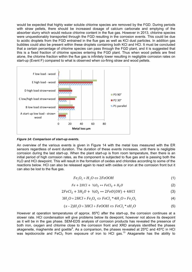
would be expected that highly water soluble chlorine species are removed by the FGD. During periods with straw pellets, there should be increased dosage of calcium carbonate and emptying of the absorber slurry which would reduce chlorine content in the flue gas. However in 2013, chlorine species were unquestionably transported through the FGD resulting in the corrosion events. This could be due to acidic droplets from the FGD entrained in the flue gas as well as KCl dust particles. In addition gas bubbles could also be present within these droplets containing both KCl and HCl. It must be concluded that a certain percentage of chlorine species can pass through the FGD plant, and it is suggested that this is a fixed fraction of chlorine species entering the FGD plant. Thus when wood pellets are fired alone, the chlorine fraction within the flue gas is infinitely lower resulting in negligible corrosion rates on start-up (Event F) compared to what is observed when co-firing straw and wood pellets.
Figure 14: Comparison of start-up events.
An overview of the various events is given in Figure 14 with the metal loss measured with the ER sensors regardless of event duration. The duration of these events increases, until there is negligible corrosion during the last start-up. When the plant start-up is from room temperature, then there is an initial period of high corrosion rates, as the component is subjected to flue gas and is passing both the H2O and HCl dewpoint. This will result in the formation of oxides and chlorides according to some of the reactions below. HCl can also be released again to react with oxides or iron at the corrosion front but it can also be lost to the flue gas.
FeOOHOHOFe 2232 (1)
2 ½ ↔ (2)
2 3 ½ ↔ 2 4 (3)
3222432 4*23 OFeOHFeClOFeHClOH (4)
OxHFeClFeOOHHClOHx 232 *3)2( (5)
However at operation temperatures of approx. 85⁰C after the start-up, the corrosion continues at a slower rate. HCl condensation will give problems below its dewpoint, however not above its dewpoint as it will be in the gas phase. SEM-EDS analysis of corrosion products has revealed the presence of both iron, oxygen and chlorine close to the corrosion front and XRD analysis identified the phases akageneite, maghemite and goetite9. As a comparison, the phases revealed at 25ºC and 45⁰C in HCl was lepidocrocite and FeCl2 from exposure of iron to HCl gas.13 Akaganeite has the ability to
0 20 40 60 80
A start up low load ‐ straw+wood
B low load straw+wood
C low/high load straw+wood
D high load straw+wood
E high load ‐ wood
F low load ‐ wood
Metal loss µm
P3 90°
P2 30°
P1 parallel
accommodate Cl in its structure and also adsorb 2-20 wt.% of water, such that it can be best described as Fe8[O,OH]16(Cl,OH)<2.
14 Therefore water is adsorbed and reacts resulting in either HCl or iron chloride formation which is also a corrosive acid. As the temperature increases, water will be gradually driven off into the flue gas, however the liquid phase will also become more acidic resulting in corrosion if it is present at the corrosion front. After a period of time, the adsorbed water is no longer present in the corrosion products and therefore there is minimal corrosion. In addition the HCl formed during reaction is released into the flue gas. Thus with longer periods above the dewpoint, HCl will gradually be lost to the flue gas and Fe-O-Cl compounds will be converted to oxides, thus reducing corrosion rates. The corrosion rates of carbon steel in saturated salt solutions have been measured where the corrosivity increases as follows:15
Thus the presence of KCl should give minimal corrosion and the cited work also revealed that FeCl2 is more corrosive than FeCl3, although no reason for this could be given. In Figure 15, the water activity to result in a saturated salt solutions as well as the water activity in the flue gas as calculated from the UNIQUAC model are illustrated. Thus if the water activity at a certain temperature for the aqueous salt is above that of the flue gas, then this salt will not be aqueous and therefore contribute minimally to corrosion.
a
b Figure 15: Water activity (activity water = relative humidity%/100) as a function of temperature for saturated salt solutions and flue gas a) taken from [5]5 and b) taken from [15]. Based on Figure 15a, CaCl2 salts and ZnCl2 salts are highly hygroscopic (as is FeCl3
16) and will form deliquescent salts at low water activities such that even at 100⁰C, these will give problems with corrosion. Alternatively KCl and NaCl require much higher water activities and will not form a saturated solution at the 15 vol% water content in the flue gas. The corrosion product FeCl2 is just slightly higher than the 15 vol.% flue gas, and as seen in Figure 15b, a mixture of KCl-FeCl2 will give a soluble salt at higher temperatures. Thus corrosion occurs at operation at 85⁰C due to the formation of these potassium chloride-iron chloride mixtures. However as the HCl is removed from the system, this corrosion will cease. Yang measured the corrosion current of carbon steel at 45⁰C below KCl deposit with an increasing humidity.18 The corrosion current was minimal until the relative humidity was increased to 70%, which would fit with Figure 15a. When the humidity was decreased to 30%, the corrosion current continued, but at a lower extent for at least 12 days. This was probably due to the fact
5 Copyright belongs to Waesseri GmbH, Power Plant Chemistry.
that KCl+FeCl2 were present as soluble salts. Thus corrosion could continue at a lower relative humidity. This is also relevant for downtime corrosion. When only wood pellets are used, then the HCl content would be much lower, thus the amount of HCl condensing on the corrosion product on component surfaces is much lower. However during Event E, there is already Cl species incorporated into the deposits as akaganeite or FeCl2 from the earlier straw-pellet firing. As a result, these can form soluble salts and thus corrosion can continue until the available chlorine is reduced. In this case it takes over two months for the corrosion rate to be minimal, which could be termed a memory effect from the straw pellets. Minimal corrosion occurred after Event F indicating that chlorine presence is too low in the flue gas to initiate corrosion. The load during this event was 40% (Figure 8), and with 100% load, a corrosion event is more likely to occur. However there was also partial load with wood+straw pellets in August, so an improvement is evident from removing straw pellets as a fuel. More data on subsequent events is required to confirm this trend. From experiences in Sweden, corrosion is observed with woodchips but then the water content would be closer to 20 vol. % 4, or other salts could be present such as CaCl2. Only Event C showed a marked difference with respect to angle of the sensor. The only factor that could be linked to this was the fluctuating load and therefore flow in the flue gas. Perhaps such an operation mode leads to more erosion due to water droplets or other particles; this needs to be further investigated when a similar corrosion profile is observed. It cannot be ruled out that the actual position of the individual sensors also has an influence as metal loss measurements across the 90⁰ sensor revealed less corrosion on the upper part. Limited downtime corrosion has been measured compared to corrosion at start-up of operation. However during this measurement period, the corrosion picture in Figure 2b has not been observed. Thus the conditions to give this appearance have not occurred. Askey et al13 reports that the corrosion rate of iron in HCl gas atmospheres doubled from 25⁰C to 45⁰C. Thus the temperature profile during the shutdown process is important. Corrosion monitoring of a small coal fired plant (with UK coal) showed that high corrosion rates occurred 7-15 days after shutdown19 which indicates that the length of stop is also relevant. The on-line ER measurements have given important data on actual corrosion rates and this data together with plant data results in a better understanding of the corrosion mechanisms. Thus it is clear that many shutdown/start-ups will influence corrosion and therefore result in shorter lifetime of components and increased maintenance. The type of fuel contributes greatly to corrosion as can be observed with wood pellets which have less HCl and less KCl compared to straw pellets. The most effective method to reduce corrosion during operation will be to increase the temperature of the flue gas to be both over the dew point of HCl but also over the dewpoint of hygroscopic salts and to avoid shutdowns. The presented corrosion monitoring system can identify optimum temperatures and procedures for minimizing corrosion, thereby extending component lifetime and improving the availability of the plant. It can predict component lifetimes thus material replacement and maintenance can be scheduled. In addition performance with alternative fuel qualities, and trial of candidate replacement materials with minimum disruption of the plant could also be undertaken.
CONCLUSIONS
The following conclusions can be drawn:
Corrosion is related to the presence of alkali chlorides, HCl and water and is initiated in a specific temperature window. The presence of hygroscopic corrosion products leads to corrosion during operation.
The precipitation of high corrosion rates have been shown to coincide with start-up of the plant. Corrosion then occurs subsequently during operation. Otherwise corrosion does not occur during operation.
The change from firing a straw-wood pellet mixture to just wood pellets (40% load) reduced the corrosion rate at start-up significantly. This is a single event, so more data is required.
The four corrosion sensors have similar trends although those that are angled towards the flue gas have more corrosion. Microscopy has verified the ER on-line measurements.
ACKNOWLEDGEMENTS
Thanks go to HOFOR - Amagerværket for fruitful discussions and allowing this paper to be published. The constructive discussions of COWI and DTU-Mekanik colleagues are also acknowledged.
REFERENCES
1. W.B.A. Sharp, D.L. Singbeil, J.R. Keiser “Superheater Corrosion Produced by Biomass Fuels” CORROSION 2012, paper no. C2012-0001308 (Houston, TX: NACE, 2011),
2. M. Montgomery, S.A. Jensen, U. Borg, O. Biede. T. Vilhelmsen, “Experience with High Temperature Corrosion as Straw-Firing power Plants in Denmark” Materials and Corrosion 62, 7 (2011) pp. 593-605.
3. L. Lindau, B. Goldschmidt ”Low temperature corrosion in bark fuelled small boilers” Värmeforsk Report M9-835 (2002 in swedish, 2008 in english.
4. M. Nordling: “Corrosion on air preheaters and economisers” Värmeforsk Report M08-815 Nr. 1235. May 2012, 5. J.P. Jensen, L.D. Fenger, N. Henriksen: “Cold-End Corrosion in Biomass and Waste Incineration Plants” Power Plant
Chemistry 2001, 2 (8) pp 469-471. 6. ELSAM F+U Rapport A2002-04.030. July 2002. 7. T. Herzog, W. Müller, W. Spiegel, J. Brell, D. Molitor, D. Schneider “Corrosion caused by dewpoint and deliquescent
salts in the boiler and flue gas cleaning” VGL: KG Thome-Kozmiensky og M. Beckmann: Energie aus Abfall Band 9 Neuruppin: TK Verlag 2012. p 429-460.
8. J.R. Kish, N.J. Stead, D.L. Singbeil, C. Reid, E. Johansson, R. Seguin, F. Preto, “Dewpoint corrosion of a coastal biomass power boiler air heater” TAPPI Engineering, Pulping and Environmental Conference August 24-27, 2008, Portland Oregon.
9. M. Montgomery, R.E Olesen, O.M. Jensen, H. Rostgaard, P. Gensmann, F. Danielsen, “Corrosion of a flue gas/gas heat exchanger in the pollution control system of a biomass fired power plant” Eurocorr 2012, Istanbul 9-14 September 2012 Paper 1504.
10. W.M.M. Huijbregts, R.G.I. Leferink “Latest advances in the understanding of acid point dewpoint corrosion: corrosion and stress corrosion cracking in combustion gas condensates” Anti Corrosion Methods and Materials Vol 51, No 3, 2004, pp 173-188.
11. L.V. Nielsen, K.V. Nielsen, “Differential ER-Technology for Measuring Degree of Accumulated Corrosion as well as Instant Corrosion Rate” CORROSION 2003, paper 03443. (Houston, TX: NACE, 2003)
12. Report from 6th Framework Programme – Horizontal Research Activities Involving SMES. Report 018207 CORRLOG “Automated corrosion sensors as on-line real time process control tools”
13. A. Askey, S.B. Lyon, G.E. Thompson, J.B. Johnson, G.C. Wood, M. Cooke, P. Sage, “The corrosion of iron and zinc by atmospheric hydrogen chloride” Corrosion Science Vol 34 2 (1993), pp. 233-247.
14. V.F. Buchwald, R.S. Clarke, “Corrosion of Fe-Ni alloys by Cl containing akaganeite (beta FeOOH): The Antartic meteorite case” American Mineralogist, Volume 74, pp 656-667, 1989.
15. L. Yang, R.T. Pabalan, L. Browning, A. Cragnolino, “Measurement of Corrosion in Saturated Solutions under Salt Deposits using Coupled Multielectrode Array Sensors” CORROSION, paper no. 02316 (Houston, TX: NACE, 2002)
16. ELSAM F+U Rapport A2002-04.030. July 2002 In Danish. 17. M.C. Iliuta, K.Thomsen, P. Rasmussen, “Modeling of heavy metal salt solubility using the extended UNIQUAC
model”, AIChE Journal, 48 11 (2002): pp. 2664-2689. 18. L.Y. Yang, R.T. Pabalan, L. Browning, D.S. Dunn, “Corrosion Behavior of Carbon steel and stainless steel materials
under salt deposits in simulated dry repository environments” Materials Research Society Proceedings 757 2003 p. I14.14.1


![diagram 5.1 [Converted] - Building Control NI · part of the flue serving an open-flued appliance. flue soot door debris collection space chimney appliance flue outlet appliance flue](https://static.documents.pub/doc/80x56/60ea4a68722f9641f22c1939/diagram-51-converted-building-control-ni-part-of-the-flue-serving-an-open-flued.jpg)
