34
TICAM Report 94-06 May 1994 Vibrations of a Spherical Shell Comparison of 3-D Elasticity and Kirchhoff Shell Theory Results Y. C. Chang & L. Demkowicz

TICAM Report 94-06May 1994
Vibrations of a Spherical Shell Comparisonof 3-D Elasticity and
Kirchhoff Shell Theory Results
Y. C. Chang & L. Demkowicz

VIBRATIONS OF A SPHERICAL SHELL.COMPARISON OF 3-D ELASTICITY ANDKIRCHHOFF SHELL THEORY RESULTS
Y. C. Chang and L. DemkowiczThe Texas Institute of Computational and Applied Mathematics
The University of Texas at AustinAustin, Texas 78712
Austin, May 1994
Abstract
Natural frequencies of a vibrating hollow, elastic sphere are determined using both 3-D elas-
ticity and Kirchhoff shell theory.
Acknowledgment: The support of this work by the Office of Naval Research under Grant
N00014-92-J-1161 is gratefully acknowledged.
Table of Contents
Table of Contents
1. Introduction 1
2. 3-D Elasticity Solution 22.1 Helmholtz Potential . . . . . . . . . . . . . . . . . . . . . . . . . . . . . . . 32.2 Separation of Variables for the Helmholtz Operator in a Spherical Domain 52.3 The Modal Characteristic Equation . . . . . . . . . . . . . 112.4 A Stable Algorithm for the Evaluation of Bessel Functions 17
3. Kirchhoff-Love shell theory solution 203.1 A review of the shell theory 203.2 Free vibration problem . . . . . . . . . . 24
4. Numerical experiments and conclusions 25

2.1 Helmholtz Potential
The motion of an isotropic, homogeneous elastic body is governed by Navier's equations
(2.4)
where u = u(x, t) is the unknown displacement field, f are prescribed body forces, p is the
density and ,\ and µ are Lame's constants. Assuming that body force f is sufficiently smooth,
we can represent them in the form.
f=Vj+VxF (2.5)
where f and F are scalar and vector potentials respectively. Assuming the same form for the
solution
u = V<I> + V x W (2.6)
With <I>and W, the unknown scalar and vector potentials, we substitute (2.6) into (2.4) to
obtain
(2.7)
here c} = J >'~2µ, C2 = ~ ' are longitudinal wave velocity and shear wave velocity, respec-
tively.
If ciV2<I> + j - ~2t~ = 0 and C~V2W +F - 8;t~ = 0 then Navier's equations (2.4) are obviously
satisfied. The nontrivial question whether every solution of Navier's equation admits a
representation (2.6) was answered positively in the completeness proof provided by Long
[5].
3

For spherical coordinates, we additionally represent the vector potential \)! [4] in the form
(2.8)
where 1 is a length factor in order to make the dimension of two terms in (2.8) the same and
Wand X are two unknown scalar-valued functions.
With body forces neglected, this leads to a final system of three decoupled wave equations
to be solved for potentials <I>, Wand x.
(2.9)
(2.10)
(2.11)
Substituting (2.8) into (2.6), we can obtain the displacement field
Displacement Field
o <I> 1[02(rx) _ V2 ]or + or2 r X
1o <I> 1 oW 102(rx)--+--+-r 00 sin 0 0<1> r oOor
1 o <I> oW 1 02(rx)Uri> = r sin 0 0<1>- 00 + r sin 0 8<1>8r
(2.12)
(2.13)
(2.14)
From the displacement-strain relationships and the constitutive equations of linear elastic
isotropic material, we can get the following stress field.
Stress Field
(2.15)
4

1 0<I> 1 02<I> 2µ 0 1 oW0'00 = ,\V
2<I> + 2µ(;: or + r2 002 ) + -:;:00 (sin 0 0<1>)
+2 l[~ 03(rx) + !(02(rx) _ rV2x)] (2.16)µ r2 o020r r Or2
2 1 a2<I> !0<I> ~ cot 0 0<I>0'",,,, = ,\V <I> + 2µ[ 2 • 20 a,,/,.2+ a + 2 ao]r SIn 'fJ l' r r
2Jl oW 02W+ r sin 0 (cot 0 0<1>- 0<1>00)
1 03(rx) 1 02(rx) 2 cot 0 02(rx)+2µ1[ 2 • 200,,/,.20 + -( 0 2 - rV X) + 2 ooa] (2.17)r SIn 'fJ r r r r r
2µ 02<I> 1 0<I> µ oW 02WO'rO = -:;:(oroO - ;: 00) - r sin 0 (0<1> - r ara<l»
+µl [~(02(rx) _ rV2X) _ !02(rx) + r~(! 02(rx))] (2.18)r 00 or2 r oOor Or r oOor
2µ 02cJ! 1 acJ! µ aw a2(rW)O'r'" = r sin 0 (oro<l> - ;: 0<1» + ;-[2 00 - oOor]
µl 0 02(rx) 2 202(rx)+ rsinB[o<l>(2 or2 - rV X) -;: o<l>or ] (2.19)
2µ 02 <I> a <I> µ aw 02 W0'0'" = r2 sin 0 (000<1> - cot 0 0<1>) + ;-(cot 0 00 - 002
1 a2W 2µ1 03(rx) a2(rx)+ sin2 0 a<l>2) + r2 sin 0 [oroOa<l> - cot 0 oro<l> ] (2.20)
2.2 Separation of Variables for the Helmholtz Operator in aSpherical Domain
By means of the separation of variables, solution of the Helmholtz equation in spherical
coordinates (r,O,<I» is reduced to solving three independent ordinary differential equations:
the Bessel equation in r, the Legendre equation in 0, and a simple, second order equation in
<1>.
5
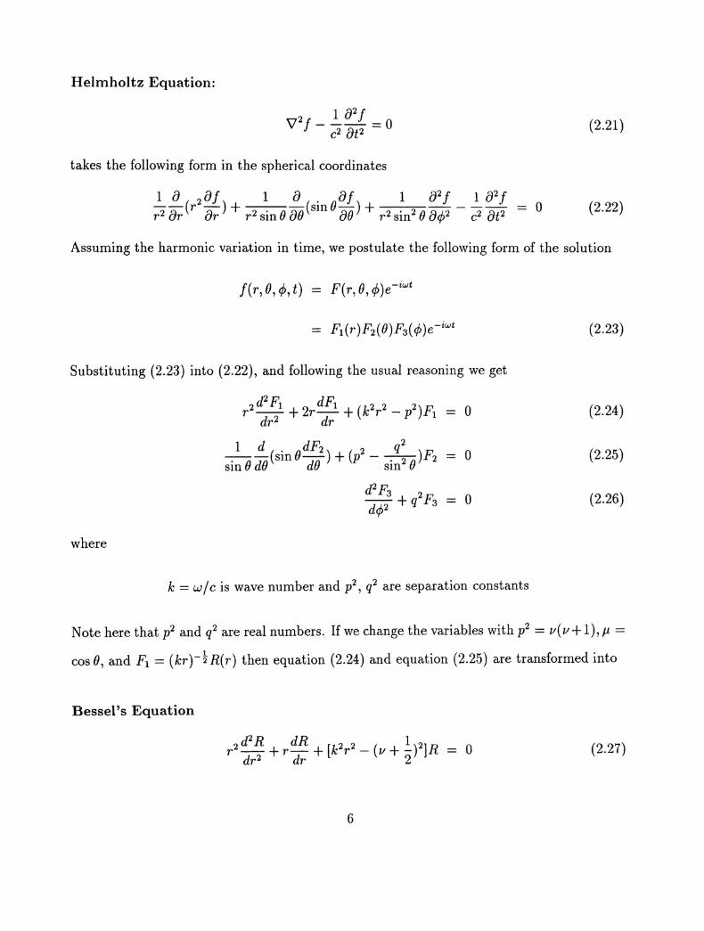
Helmholtz Equation:
(2.21 )
takes the following form in the spherical coordinates
Assuming the harmonic variation in time, we postulate the following form of the solution
j(r,O,<I>,t) = F(r,B,<I»e-iwt
Substituting (2.23) into (2.22), and following the usual reasoning we get
(2.23)
where
r2 d2Fl + 2r dF1 + (k2r2 _ p2)Fl
dr2 dro
o
o
(2.24)
(2.25)
(2.26)
k = w / c is wave number and p2, q2 are separation constants
Note here that p2 and q2 are real numbers. If we change the variables with p2 = v(v+ 1), µ =
cosO, and Fl = (krttR(r) then equation (2.24) and equation (2.25) are transformed into
Bessel's Equation
d2R dR 1r2_ + r- + [k2r2 - (v + - )2]Rdr2 dr 2
6
a (2.27)

and
Legendre's Equation
2 d2F2 dF2 m2
(1- µ )- - 2µ- + [V(V + 1)- ]F2 = 0dµ2 dµ 1_ µ2 (2.28)
Since F3 must be a single valued function periodic with period 211',separation constant q
must be an integer, say m. For the special case q=O, solution of (2.26) reduces to a constant
function. For q =f. 0, solution F3 is a linear combination of eiqr/> and e-iqr/>. Next, applying
the Frobenius methods to solve the Legendre's equation we find out that a necessary and
sufficient condition for the solution to exist is that v must be a nonnegative integer. The
corresponding solution is then the classical associated Legendre functions.
Summarizing, we get the final solution in the form
(2.29)
where
P;:-(µ) and Q:;:(µ) are associated Legendre functions
In+l/2(kr) is Bessel function of first kind and n+l/2 order
Yn+l/2(kr) is Bessel function of second kind and n+l/2 order
Associated Legendre function Q:;: is singular at Il = ±1, therefore we exclude it from the
solution of the sphere problem. We can express then the general Helmholtz potentials as
x
Z~i)( ar )P;:-( cos 0) exp[i(m<l> - wt)]
Z~i)(/3r)P;:-(cos 0) exp[i(m<l>- wt)]
7
(2.30)
(2.31 )
(2.32)

where
(2.33)
(2.34)
(2.35)
jn(kr) and Yn(kr) are Spherical Bessel functions
The displacement field is derived by substituting equations (2.30), (2.31), and (2.32) into
equations (2.12), (2.13), and (2.14)
Ur = ![Uii)(ar) + lUJi) (/3r)]P:(cos 0) exp[i(m<l> - wt)] (2.36)r
1 (i) n + mUo = -{Y; (ar)[ncotOP:(cosO) - . 0 P:"l(cosO)]r SIn .
+V}i)(/3r) ~mBP:(cosB) + ly;(i)(/3r)[ncotOP;:-(cosO)SIn
- n :- ; P:"l (COSO)]} exp[i(m<l> - wt)] (2.37)SIn
1 () im (")uri> = -{Y;' (ar)~P;:-(cosB) - rV2' (/3r)[n cot OP;:-(cos 0)r SIn
n :- ; P:"l (cos B)] + ly;(i)(/3r) ~mBP:( cos On exp[i(m<l> - wt)] (2.38)SIn SIn
where
(2.40)
(2.41 )
8

u1i), y;(i), W1(i) = y;(i) correspond to function cJ!
UJi) = 0, V;(il, J;VJi) = V;(i) correspond to function W
UJi), Y;(i), lVJi) = Y;(i) correspond to function X
Using the usual displacement-strain relations and the constitutive equations of a linear
isotropic elastic material, we get the following stress field represented in terms of scalar
functions <I>, W, and x.
Stress Field
(') zm+(n + m) cos OP:"l (cos 0)] + T2; (/3r)~{) [(n - 1) cos OP;:-( cos ())SIn
+(m + n) cos BP:"l (cos B)]} exp[i( m<l>- wt)]
2µ (') A (') 12{T3~ (ar)P;:-(cos ()) + T3~(ar)~B [(n cos2 0 - m2)p;:-(cos 0)r ~n
C) zm-(n + m) cos OP:"l (cos B)] + T3; (/3r)~B [-(n - 1) cos OP:( cos 0)SIn
. exp[i(m<l>- wt)]
9
(2.42)
(2.43)
(2.44)
2µ { (i)()[ m( n + mO'rO = "2 T41 ar ncotOPn cosO) -. P::"l(cosO)]r SIll0
+Tl;)(/3r) ~mop;:-(cosO) + IT1~\/3r)SIn
. [n cot 0P: (cos 0) - n:-; P:"l (cos B)]} exp [i(m <I> - wt)] (2.45)SIn
2µ { (i)( ) im m( ) (i) 1 mO'rr/> = "2 TSI ar ~Pn cosO - TS2 (/3r)~[ncosOPn (cosO)r SIn SIll
(") zm-(n + m)P::"l (cos B)] + ITs; ((3r)~P:( cos OnSIll
. exp[i(m<l> - wi)] (2.46)
2µ (i) imO'Or/> = "2{T61 (ar )--:---za[( n - 1) cos OP:( cos 0) - (n + m )P:"l (cos 0)]r SIn
() 1 n(n - 1)+T6~ (/3r)~[( 2 sin20 + n - m2)p;:-(cosO)
SIn
() zm-( n + m) cos OP:"l (cos 0)] + IT6; (/3r )--:---za[(n - 1) cos OP:( cos 0)SIn
-( n + m )P::" 1 (COS O)]} exp[i( m<l>- wt)]
where
T12(ar) = (n2 - n - ~/32r2)Z~i)(ar) + 2arZ~~1(ar)
T1~(/3r) = n(n + l)[(n -l)Z~i)(/3r) - /3rZ~~l(/3r)]
TJ~)(ar) = (_n2 - ~/32r2 + a2r2)Z~i)(ar) - arZ~~l (ar)
TJ2(ar) = Z~i\ar), TJ;) (/3) = r Z~i) (/3r)
TJ~)(/3r) = _(n2 + n)[nZ~i)(/3r) - /3rZ~~l(/3r)]
TJ~)(/3r) = (n + l)Z~i)(/3r) - /3rZ~~l(/3r)
10
(2.4 7)
(2.48)
(2.49)
(2.50)
(2.51 )
(2.52)
(2.53)
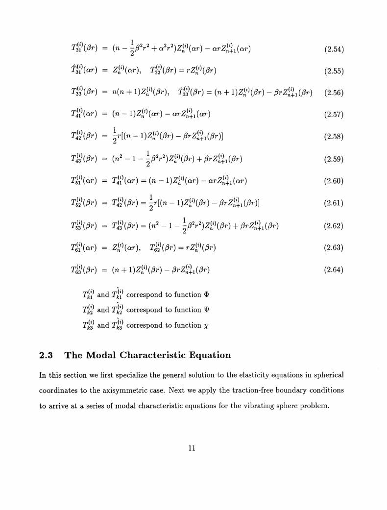
TJ2(/3r) = (n - ~/32r2 + a2r2)Z~i)(ar) - arZ~~l(ar) (2.54)
TJ~)(ar) = Z~i)(ar), TJ;) (/3r) = r Z~i) (/3r) (2.55)
TJ~)(/3r) = n(n + l)Z~i)(/3r), TJ~)(/3r) = (n + l)Z~i)(/3r) - /3rZ~~l(/3r) (2.56)
TJ~)(ar) = (n - l)Z~i)(ar) - arZ~~l(ar) (2.57)
TJ;) (/3r) = !r[(n -l)Z~i)(/3r) - /3rZ~~l(/3r)] (2.58)2
TJ~)(/3r) = (n2 - 1 - ~/32r2)Z~i)(/3r) + /3rZ~~l(/3r) (2.59)
TJ2(ar) = TJ~)(ar) = (n -l)Z~i)(ar) - arZ~~l(ar) (2.60)
TJ;\/3r) = TJ;)(/3r) = !r[(n - l)Z~i)(/3r) - /3rZ~~l(/3r)] (2.61 )2
TJ~)(/3r) = TJ~)(/3r) = (n2 - 1- ~/32r2)Z~i)(/3r) + /3rZ~~l(/3r) (2.62)
TJ~)(ar) = Z~i)(ar), TJ;)(/3r) = rZ~i)(/3r) (2.63)
TJ~)(/3r) = (n + l)Z~i)(/3r) - /3rZ~~I(/3r) (2.64)
T~2 and T~~)correspond to function cJ!
T1;) and T1;) correspond to function W
T1~ and T1~ correspond to function X
2.3 The Modal Characteristic Equation
In this section we first specialize the general solution to the elasticity equations in spherical
coordinates to the axisymmetric case. Next we apply the traction-free boundary conditions
to arrive at a series of modal characteristic equations for the vibrating sphere problem.
11

Assumption on the axisymmetric form of the vibrations (the axis of symmetry coincides
with the vertical axis B=o) implies elimination of the <I>-componentof the displacement field,
ur/>=O, and all derivatives with respect to the <I> variable, :r/> = O. Consequently, q=O in
equation (2.26), solution F3 reduces to a constant function and m=o in Legendre's equation
(2.23), i.e. the associated Legendre functions P::"(µ) reduce just to the Legendre polynomials
Summarizing, the formulas for Helmholtz potentials in the axisymmetric case, reduce to
Z~i)( ar )Pn( cos B) exp[ -iwt]
z~i)(/3r) exp[ -iwt]
(2.65)
(2.66)
x (2.67)
with
z(1)n (2.68)
(2.69)
where
Pn are Legendre polynomials
In+l are Bessel functions of order n + ~2
The corresponding displacement field takes the simplified form
12
(2.70)

Displacement Field
a <I> 1[02(rx) n2]- + - rv Xar !L?
10cJ! 1 a2(rx)--+r 00 r oOor
a
and the corresponding stress field looks as follows
(2.71 )
(2.72)
(2.73)
Stress Field
2 02 <I> 0 02(rx) 2(2.74)O'rr = ,\V <I>+ 2Jl or2 + 2µ1 or [ ar2 - rV X]
2 18<I> 1 02cJ! 1 83(rx) 1 a2(rx) 2(2.75)0'00 = "V <I>+ 2µ(;: ar + r2 0(2) + 2µ1[r2 aB20r +;:( ar2 ) - rV X)]
2 1 acJ! 1 acJ! 1 a2(rx) 2O'r/>r/> = "V <I>+2µ[-a+2"cotOoo]+2µ1[-( a 2 -rV X)r r r r r
+cot B 02(rx)](2.76)r2 oOOr
arB = 2µ (a2cJ! _ ~ acJ!) + µl [~( a2(rx) _ rV2x) _ 1 a2(rx)r arao r aB r aB ar2 l' aoar
a (1 a2(rx)] (2.77)+r- ar r ooar
O'rr/> = 0 (2.78)
O'or/> = 0 (2.79)
Substituting <I>,W, and X in (2.65), (2.66), and (2.67) into the stress field above, we arrive
at the final formulas for stresses in terms of Bessel functions and Legendre polynomials
13

Stress Field
O'rr = 2~[T12(ar) + lT1(;\/3r)] Pn (cos 0) exp(-iwt) (2.80)r2µ C) A (") 1
0'00 = 2{T2~ (ar)Pn(cosO) +T2~ (ar)""72(j[-ncos2OPn(COsO)r SIn
+ncosOPn_I(COsO)] + ITJ;)(/3r)Pn(cosB) + lTJ~)(/3r)~SIn 0
.[( -n cos2 O)Pn( cos 0) + n cos OPn-1 (cos O)]} exp( -iwt) (2.81 )
2µ C) A (") 1O'r/>r/> = 2{T3~ (ar)Pn(cosB) +T3~ (ar)""72(j[ncos2OPn(cosO)r ~n
(") AC) 1-n cos OPn_1(cosB)] + IT3; (/3r)Pn(cosO) + IT3; (/3r)~SIn B
·[(n cos2 O)Pn( cos 0) - n cos OPn-1 (cos B)]} exp( -iwt) (2.82)
2µ (i) nO'rO = 2{T41 (ar)[ncot BPn(COS 0) - ~Pn_l(cosB)]r SIn
+lT1~)(/3r) . [n cot OPn( cos 0) - .n 0 Pn-1 (COSB)]} exp( -iwt) (2.83)SIn
O'rr/> = O'Or/> = 0 (2.84)
where:
T1~\ar) = (n2 - n - ~/32r2)Z~i)(ar) + 2arZ~~1 (ar) (2.85)
T1(;)(/3r) = n(n + l)[(n - l)Z~i)(/3r) - /3rZ~~l(/3r)] (2.86)
TJ~)(ar) = (_n2 - ~/32r2 + a2r2)Z~i)(ar) - arZ~~l (ar) (2.87)
TJ~)(ar) = Z~i)(ar) (2.88)
TJ;) (/3r) = _(n2 + n)[nZ~i)(fir) - /3rZ~~l(fir)] (2.89)
14

'i'J~)(/3r) = (n + l)Z~i)(/3r) - /3rZ~~l(/3r)] (2.90)
TJ2(/3r) = (n - ~/32r2 + a2r2)Z~i)(ar) - arZ~~l(ar) (2.91)
'i'J2(ar) = Z~i)(ar) (2.92)
TJ~)(/3r) = n(n + l)Z~i)(/3r) (2.93)
'i'J~)(/3r) = (n + l)Z~i)(/3r) - /3rZ~~l(/3r) (2.94)
TJ2(ar) = (n - l)Z~i)(ar) - arZ~~l (ar) (2.95)
TJ~)(,8r) = (n2 - 1 - ~/32r2)Z~i)(/3r) + /3rZ~~l(/3r) (2.96)
Traction Boundary Conditions
The boundary conditions on the inner surface and on the outer surface of the hollow sphere
are
where
0' Tr = 0' rr/> = 0' rO = 0 at r = r0
ri : inner radius
ro : outer radius
(2.97)
(2.98)
Boundary condition O'rr/> = 0 both on the inner and outer surfaces, is automatically satisfied.
The remaining four boundary conditions contribute with the following four equations in
15
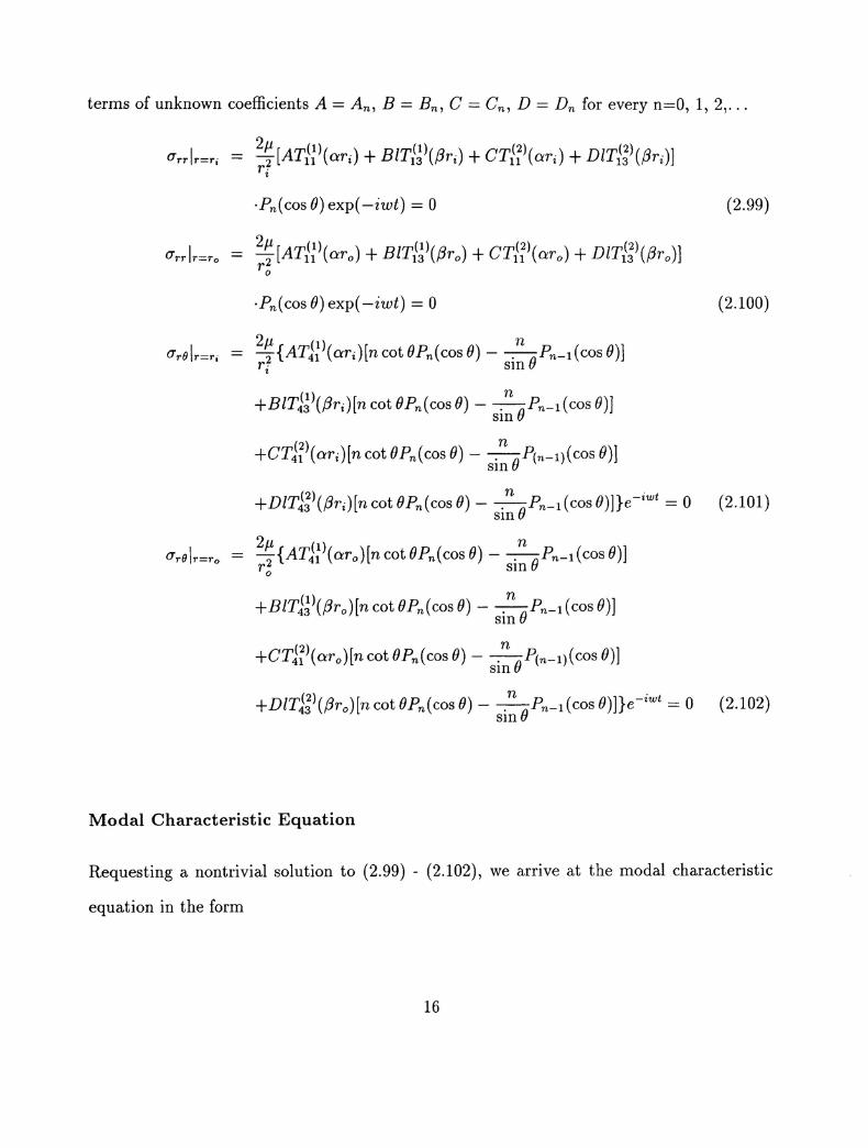
terms of unknown coefficients A = An, B = Bn, C = Cn, D = Dn for every n=o, 1, 2, ...
I - 2µ [AT(l)( ) 1 (1)( ) C (2)() (2)O'rr r=rj - 2 n ari + B T13 /3ri + Tn ari + DIT13 (,sri)]r·,
·Pn( cos 0) exp( -iwt) = a (2.99)
O'rrlr=ro = 2~ [AT{:)(aro) + BITg)(/3ro) + CTR)(aro) + DIT};) (/3ro)]ro
·Pn( cos 0) exp( -iwt) = 0 (2.100)
_ 2µ (1) nO'rO!r=rj - 2{AT41 (ari)[ncotOPn(cosO) - ~Pn_1(COSO)]
ri SIn
+BITJ~)(/3ri)[ncotOPn(COSO) - .n BPn-1(cosO)]SIn
(2) n+CT41 (ari)[ncotOPn(cosO) - ~P(n-1)(cosB)]SIn
(2) n . (2.101)+DIT43 (/3rd[n cot OPn( cos 0) - ~Pn-1 (cos O)]}e-,wt = aSIn
_ 2µ (1) nO'rO!r=ro - 2{AT41 (aro)[n cot BPn(COS 0) - ~Pn_1(cosB)]
roSIn
+BITJ~)(/3ro)[ncotOPn(COSO) - .n OPn-1(cosO)]SIn
+CTJ;)(aro)[ncot OPn(cos0) - .n o P(n-1) (cos 0)]SIn
(2) n . (2.102)+DIT43 (/3ro)[ncot OPn(cos 0) - ~Pn_1(CosO)]}e-,wt = aSIn
Modal Characteristic Equation
Requesting a nontrivial solution to (2.99) - (2.102), we arrive at the modal characteristic
equation in the form
16

Tg)(ari)(1) ( )TIl aro
(1)( )T4l ari(1)( )T4I aro
Tg)(OTi)(2) ( )Tn OTo
Tl;)(ari)Tl;)(aro)
= 0 for n > a (2.103)
where
a = w, /3 = W, Cl = J'\ + 2µ, C2 = fE~ ~ p Vp
(2.104 )
Note that in case n=o equation (2.101) and equation (2.102) are automatically satisfied, so
the determinant is 2 by 2.
2.4 A Stable Algorithm for the Evaluation of Bessel Functions
Many algorithms have been proposed to evaluate Bessel functions of fractional order. Here
we adopt Steed's method and Temme's Series. The Steed method described in [6] consists
in calculating Jv, J~, Yv, and Y: using the following three relations
Wronskian Relation
First Continued Fraction (CFl)
(2.105)
J'vIv = JvV Jv+l---x Jv
vIIx 2(v + l)jx- 2(v + l)jx- ...
17
(2.106)

The rate of convergence for CFl is determined by the position of the turning point Xtp =
vv(v + 1) ~ v. If x <~ Xtp, the convergence of CFl is very rapid. If x >~ Xtp, each
iteration of CFl effectively increases v by one until x <~ Xtp.
Second Continued Fraction (CF2)
. _ J~+ iY: 1 . i (1/2)2 - v2 (3/2)2 - v2
p + zq = Jv + iYv = - 2x + z + ;- 2(x + i)+ 2(x + 2i)+ ...
If x >~ Xtp then equation (2.107) converges rapidly.
(2.107)
For x not small, we can ensure that x >~ Xtp by stable downward recurrence Jv and J~ to
a value v = µ <~ x. The initial values for the recurrence are
J~_l
The downward recurrence relations are
J~_l
arbitrary
V J'-Jv+ vxv-I +J-Jv-l v
x
(2.108)
(2.109)
(2.110)
(2.111)
Since CF2 is evaluated at v = µ, from equation (2.105), (2.106), and (2.107) we can solve
the equation for four unknowns, Jµ, J~, Yµ, and Y~
J _ ±( W1/2
(2.112)µ - q+'Y(p-fµ))
J~ = jµJµ (2.113)
Yµ = 'YJµ (2.114)
y' = y. (p + !L) (2.115)µ µ 'Y
18
where the sign of Jµ is the same as that of the initial Jv in equation (2.108) and
,= P - fµq
(2.116)
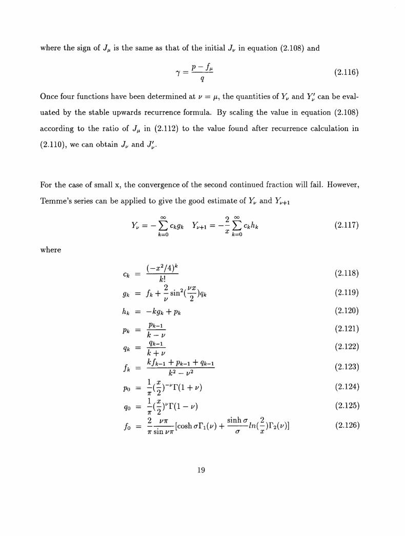
Once four functions have been determined at v = µ, the quantities of Yv and Y: can be eval-
uated by the stable upwards recurrence formula. By scaling the value in equation (2.108)
according to the ratio of Jµ in (2.112) to the value found after recurrence calculation in
(2.110), we can obtain Jv and J~.
For the case of small x, the convergence of the second continued fraction will fail. However,
Temme's series can be applied to give the good estimate of Yv and Yv+1
where
(2.117)
gk
Pk
Po
fo
(_x2/4)kk!
2 . 2(VX)fk + ~SIn 2" qk
-kgk + Pk
Pk-lk-vqk-l
k+vkfk-l + Pk-l + qk-l
k2 - v2
1 x;(2tvql + v)
!(~tf(l - v)11' 22 V11' sinh 0' 2--;--[coshO'fl(v) + -In( - )f2(v)]11' SIn V11' 0' x
19
(2.118)
(2.119)
(2.120)
(2.121)
(2.122)
(2.123)
(2.124)
(2.125)
(2.126)

0'2
vIn-x
1 [1 12v f(l - v) - r(l + 1/)]1 1 12"[n/l \ + nil , \]
(2.127)
(2.128)
(2.129)
For more detail of these methods see reference [6].
3. Kirchhoff-Love shell theory solution
Following [1], we review the classical Kirchhoff-Love theory for thin shells and derive the
shell equations in spherical coordinates under the simplifying assumption of axisymmetric
vibrations. As in the case of 3-D continuum, we arrive finally at a series of characteristic
modal equations.
3.1 A review of the shell theory
In order to derive the equations of motion of thin elastic shells, Love introduced the following
four assumptions.
• !l < < 1, i.e., thickness hover midsurface radius a is very small.a
• ur/h,uo/h, and ur/>/h «1, i.e., the displacement is small compared with thickness.
• O'rr is negligible.
• Fibers in the radial direction remain undeformed during the motion.
Based on these assumptions, if we consider the axisymmetric vibrations only, we can express
the components of the displacement vector in terms of the displacements of middle surface
(3.1)
20

tio = (1 + ~)Uo _ ~ aUra a ao
where x = r - a, and Ur a.s well as Uo are functions of 0 only.
The kinetic energy can be expressed as follows:
(3.2)
(3.3)
After neglecting x in comparison to midsurface radius a, we can obtain the total kinetic
energy in terms of Ur and uo.
(3.4)
Neglecting the effects of rotatory inertia and plugging (3.1) and (3.2) into (3.4), we can
simplify the total kinetic energy to the following form
r .2 ·2T = 11'Psha2 Jo (Ur + Uo ) sin 0 dO (3.5)
Nonvanishing components of strain in spherica.l coordinates can be expressed in terms of Ur
and Uo as
coo ~ouoa + x ( ao + ur)
1a + x (cot OUo + ur)
(3.6)
(3.7)
If we substitute (3.1) and (3.2) into (3.6) and (3.7), then we get
1 auo x BUo a2Ur
coo = a + x ( ao + Ur) + a( a + x) ( 00 - a02 )
1 x o~cr/>r/>= -(coteUo + Ur) + ( ) cote(Uo - ae)a+x aa+x
The nonvanishing components of stress in terms of coo and cr/>r/>are
E(coo + vCr/>r/»- v-
E(cr/>r/>+ VC()O)
21
(3.8)
(3.9)
(3.10)
(3.11)
(3.12)
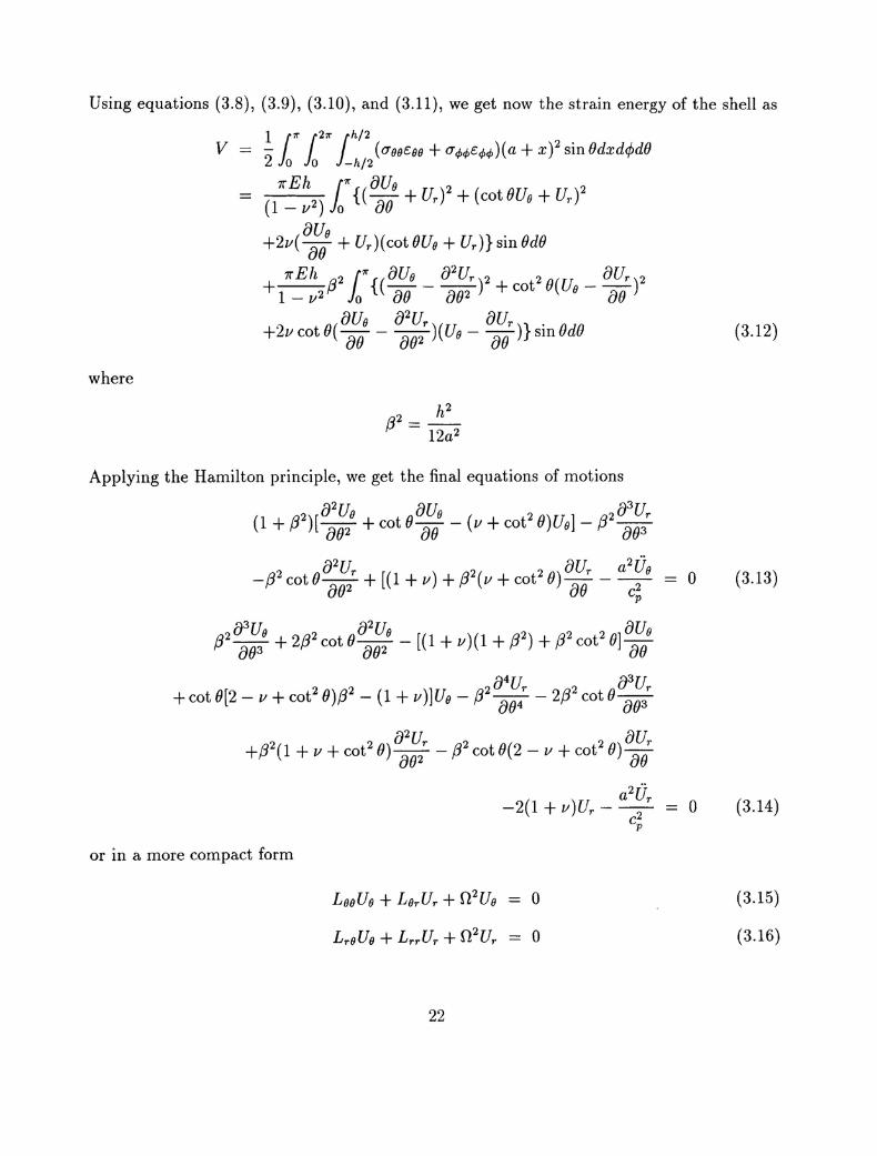
Using equations (3.8), (3.9), (3.10), and (3.11), we get now the strain energy of the shell as
1 !n7r !n27rjh/2V = - (O'oocoo + O'r/>r/>Cr/>r/»(a+ x)2 sinOdxd<l>dO
2 0 0 -h/2
11'Eh r{(oUo )2 ( )2= (1 - v2) Jo 00 + Ur + cotBUo + Ur
+2v( a:oo + Ur)( cot OUn + Ur)} sin OdO
11'Eh a2 r{(auo _ a2Ur)2 20(11 _ aUr)2+ 1 - V2fJ Jo ao a02 + cot n ao
oUO 02Ur )( OUr)} . B+2v cot O( 00 - OB2 Uo - 00 SIn dO
where
Applying the Hamilton principle, we get the final equations of motions
(3.13)o
( a2)[82Uo oUO ( 2 )] 203Ur1 + fJ a02 + cot 0 00 - v + cot 0 Uo - /3 a03
2 02Ur [( ) 2( 2 ) oUr a2Uo- /3 cot 0 OB2 + 1 + v + /3 V + cot 0 00 - T2 a3UO 2 82UO [( ( 2) 2 2] oUO/3 003 + 2/3 cot 0 002 - 1 + v) 1 + /3 + /3 cot 0 ao
0411 a311+ cot 0[2 - V + cot2 0)/32 - (1 + V)]UO - /32 a04r - 2/32cot 0 a03r
2 2 a2Ur 2 ( 2 aUr+/3 (1 + V + cot 0) 002 - /3 cotO 2 - V + cot B) aoa2(j
-2(1 + v)Ur - -i- = 0 (3.14)Cp
or in a more compact form
ao
(3.15)
(3.16)
22

where
Loo
and
2 21d2 21(1+ /3 ){(1-1J )2-(1-1J )2 + (1- vnd1J2
1 d 2d 2(1 -1J2)2{[/32(1 - v) - (1+ v)- + /3 -V }d1J d1J 11
dId 1-([/32(1 - v) - (1 + v)]-(l _1J2)2 + /32V2-(1 _1J2)2}
d1J 11d1J
-/32V~ - /32(1 - v)V~ - 2(1 + v)
(3.17)
(3.18)
(3.19)
(3.20)
V2 = ~(1 - 1J2)~11 d1J d1J
The following notation has been used
• a : the radius of the middle surface of the shell,
• E, v : the Young modulus and Poisson ratio,
• h : the thickness of the shell,
• 1J = cos 0,
• n : dimensionless frequency of the shell,
• c : wave velocity,
• Cp : the low frequency phase velocity of compressional waves in an elastic plate,
• w : the frequency,
• k : the wave number.
23
(3.21 )

3.2 Free vibration problem
The displacement field admits the spectral representation in terms of Legendre polynomials:
00
Ur(1]) = 2::UrnPn(1])exp(-iwt)n=O
()~ 2 1 dPnUo 1] = L.J UOn(1-1] )2d exp( -iwt)n=O 1]
By substituting (3.22) and (3.23) into (3.13) and (3.14), we can obtain
(3.22)
(3.23)
o (3.24)
(3.25)
For a nontrivial solution of equation (3.24) and equation (3.25), the characteristic equation
for natural frequencies n must be satisfied
where
or, equivalently
24
o (3.27)
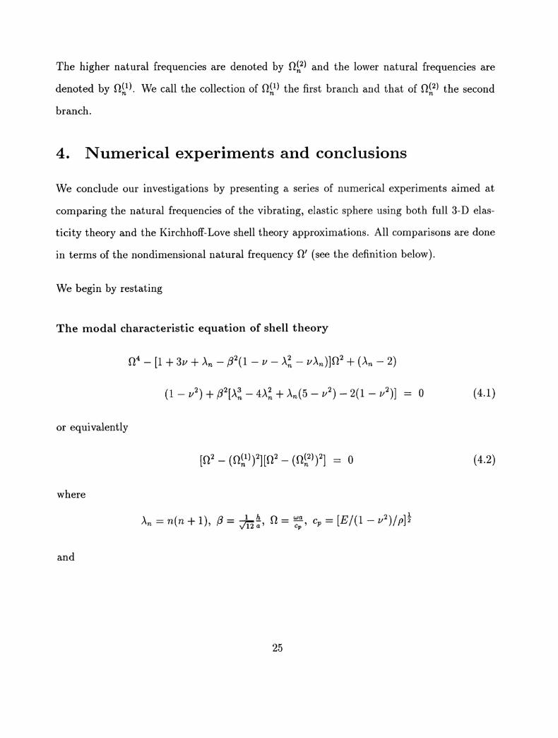
The higher natural frequencies are denoted by 0~2) and the lower natural frequencies are
denoted by 0~1). We call the collection of O~l) the first branch and that of 0~2) the second
branch.
4. Numerical experiments and conclusions
We conclude our investigations by presenting a series of numerical experiments aimed at
comparing the natural frequencies of the vibrating, elastic sphere using both full 3-D elas-
ticity theory and the Kirchhoff-Love shell theory approximations. All comparisons are done
in terms of the nondimensional natural frequency 0' (see the definition below).
We begin by restating
The modal characteristic equation of shell theory
04 - [1 + 3v + An - /32(1 - V - A~ - VAn)]02 + (An - 2)
(1 - v2) + /32[A~ - 4A~ + An(5 - v2
) - 2(1 - v2)]
or equivalently
a (4.1)
o (4.2)
where
and
25
The modal characteristic equation of 3-D theory
(1)( ) (1)(/3) (2)( ) (2)( )Tn ari T13 ri Tn ari T13 /3ri(1)( ) (1)( ) (2)( ) (2)(/3)6. - I Tn aro T13 /3ro Tn aro T13 ro I - 0 £ 0
n - (1) (1) (2) (2) - or n >T4l (ari) T43 (/3rd T4l (ari) T43 (/3ri)TJ:)( ar 0) TJ~)(/3r 0) TJ;) (ar 0) TJ~)(/3r 0)
(1)( ) (2)( )6. - I Tn ar i Tn ari I - 0 £ - an - (1) (2) - or n -Tn (ar 0) Tn (ar 0)
(4.3)
(4.4)
(4.5)
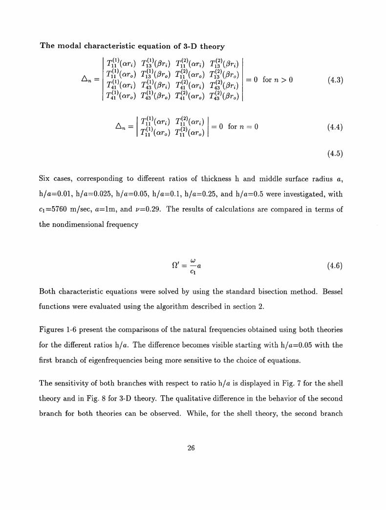
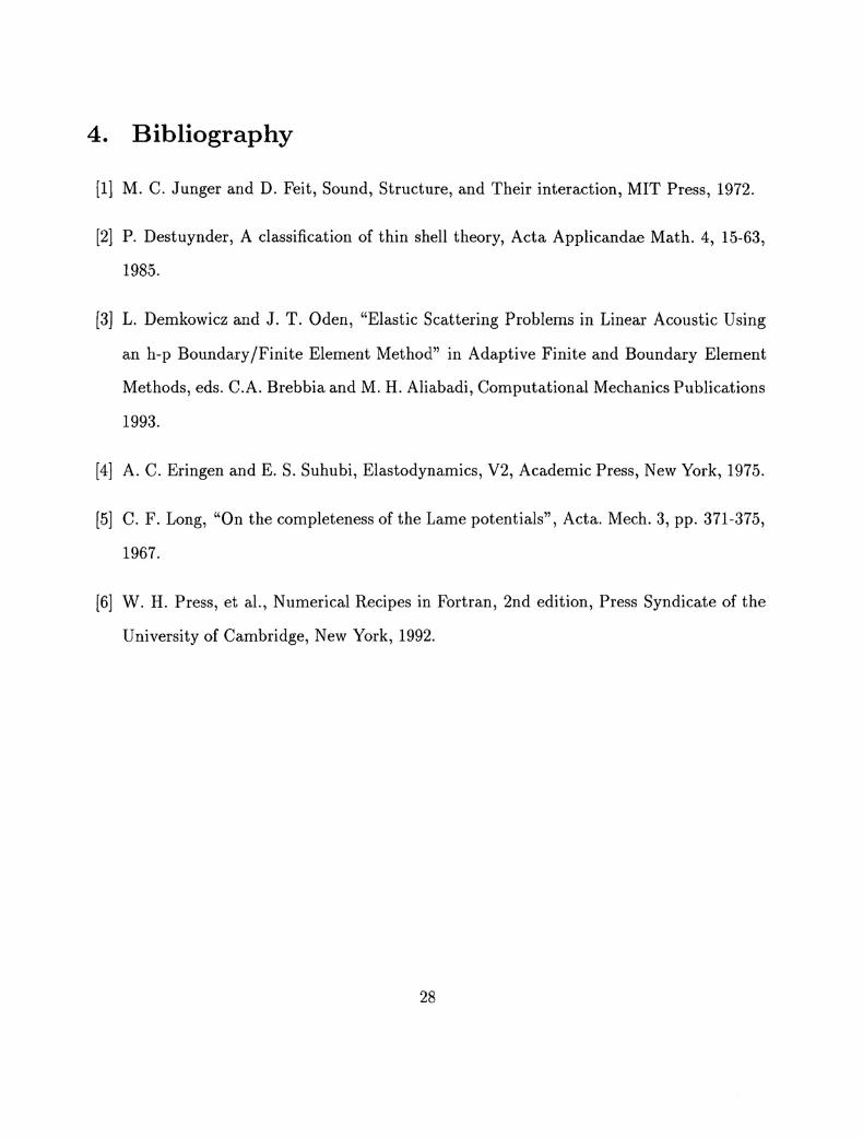
Six cases, corresponding to different ratios of thickness h and middle surface radius a,
h/a=O.Ol, h/a=0.025, h/a=0.05, h/a=O.l, h/a=O.25, and h/a=0.5 were investigated, with
Cl =5760 m/sec, a=lm, and v=0.29. The results of calculations are compared in terms of
the nondimensional frequency
(4.6)
Both characteristic equations were solved by using the standard bisection method. Bessel
functions were evaluated using the algorithm described in section 2.
Figures 1-6 present the comparisons of the natural frequencies obtained using both theories
for the different ratios h/ a. The difference becomes visible starting with h/ a=0.05 with the
first branch of eigenfrequencies being more sensitive to the choice of equations.
The sensitivity of both branches with respect to ratio h/ a is displayed in Fig. 7 for the shell
theory and in Fig. 8 for 3-D theory. The qualitative difference in the behavior of the second
branch for both theories can be observed. While, for the shell theory, the second branch
26

moves up with h/a decreasing, the same branch for the 3-D results is moving down getting
closer to the first branch.
Finally, in Fig. 9 we indicate the qualitative difference between the two characteristic equa-
tions. While equation (4.1), for n ~ 1, has two double eigenfrequencies only, equation (4.3)
has infinitely many solutions. This corresponds to the presence of multiple branches, with
only the first two branches reproduced by the shell theory. Fig. 10 presents the variation of
determinant of (4.3) for h/ a=o.Ol indicating the existence of the higher natural frequencies
corresponding to branches of higher order.
27
4. Bibliography
[1] M. C. Junger and D. Feit, Sound, Structure, and Their interaction, MIT Press, 1972.
[2] P. Destuynder, A classification of thin shell theory, Acta Applicandae Math. 4, 15-63,
1985.
[3] L. Demkowicz and J. T. Oden, "Elastic Scattering Problems in Linear Acoustic Using
an h-p Boundary/Finite Element Method" in Adaptive Finite and Boundary Element
Methods, eds. C.A. Brebbia and M. H. Aliabadi, Computational Mechanics Publications
1993.
[4] A. C. Eringen and E. S. Suhubi, Elastodynamics, V2, Academic Press, New York, 1975.
[5] C. F. Long, "On the completeness of the Lame potentials", Acta. Mech. 3, pp. 371-375,
1967.
[6] W. H. Press, et aI., Numerical Recipes in Fortran, 2nd edition, Press Syndicate of the
University of Cambridge, New York, 1992.
28

Figure 1: h/a = 0.01100
....... {}'1 (3D theory)
- {}'2 (3D theory)
l!. {}'1 (shell theory)
X {}'2 (shell theory)
100
9-ij' 10c:Q)::Ja-ll!
OJ..
"iiic:0·iiic:
~'Cc:0Z
0.1
10
0.1
o 5 10
N
15 20 25
Figure 2: h/a = 0.025100
....... 0'1 (3D theory)
- {}'2 (3D theory)
(:,. 0'1 (shell theory)
x 0'2 (shell theory)
100
9-ij'c:Q)
~u:(ijc:o"iiic:Q)
E'Cc:oZ
10
0.1
10
0.1
o 5 10
N
15 20 25
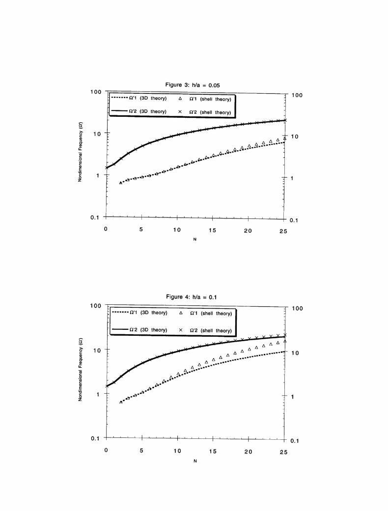
Figure 3: h/a = 0.05100
....... 0'1 (3D theory) 6 0'1 (shell theory)100
- 0'2 (3D theory) x 0'2 (shell theory)
9->- 100c:Q)
"C"l!!u.."iiic:0'iiic:Q)
E'6c:0Z
l'; l'; l'; l'; l';A A ~ •• ~ ••••••••••••••••
~.-'l ••"'••" ••.,.~.~.~.
O·b-
A• .:'I·e.o<!I·o<!I·O•
10
0.1
o 5 10 15 20 25
0.1
N
Figure 4: h/a = 0.1
100
x (l'2 (shell theory)
6 (l'1 (shell theory)
6 l'; l'; 6
6 l'; 66 l'; 6••••••••••• ···················.,- 1 0
A D. ••••••••A. c-..···&-g •• -
~ .....:'I.~.~.~.
- (l'2 (3D theory)
....... 0'1 (3D theory)100
9->- 100c:Q)
"C"l!!u..
"iiic:0'iiic:Q)
E'6c:0Z
0,1 0.1
o 5 10 15 20 25
N

Figure 5: h/a = 0.25100
100
Q.>-oc:
'""CT
'"It(ijc:o·iiic:
'"Eiic:oZ
10x X6. t:;
" •..•••........................................
6. •••••••A ••w.·4·--
p •.~.
10
.. ..... 0'1 (3D theory) t:; 0'1 (shell theory)
- 0'2 (3D theory) x 0'2 (shell theory)
0.1
o 5 10 15 20 25
0.1
N
Figure 6: h/a = 0.5
100
10
x x x x x xx x x x
x xxxx
x6. t:; 6. 6. 6. t:; 6. 6. 6. 6. 6. 6.
-...................................................
...A ••
L.l ......te·"..r...
100
Q.>- 100c:
'""CT
'"It(ijc:0'iiic:'"Eiic:0Z
--- .... 0'1 (3D theory) 6. 0'1 (shell theory)
- 0'2 (3D theory) x 0'2 (shell theory)
0.1 0.1o 5 10 15 20 25
N
Figure 7: Shell theory
10
(1'1 (h/a=O.Ol)
(1'2
'\....- .-
•••• (1'1 (hla=O.5) ••••••.. .,- ...... .. ...... .... ......... •••• (1'1 (h/a=O.ll •• ••••.. ... .... '\: .. ....
I • .-. . .-o' ••• •••• (1'1 (h/a=O.05).. .. ..-. .- .-! ... ..... ....../ :........ . ,.• .e ._- ••••••••••• , ••• 1•••••••••••••••••••••••••
•
109-1';'cCD:0aCDu:coco.;;;cCDE'i5coZ
o 5 10 15 20 25N
Figure 8: 3-D theory
9- 10'""cCD:0aCDu:coc:0'iiic:CDE'i5c:0z
1
..•••...•::::::::::::::~........ . ..- .- .-.... ..- .....- .- .-.... ..- ..-" .- ..-....~ ..,~ .,-. . ............ ~
··(1'1 (hla=O.5) •• i'1"(h/a=O'J~. . "'-
••• ••• •••• (1'1 (h/a=O.05)• •• .. .0·. . .. .... . . ... . . .-. .. .. ...,.: . "-: .0 •••• •••••••• (1'1 (h/a=O.01)fj' ,.' .,1lJ1I!I ••••••••••
I' "'.:•••••••••••••.. .:.:: ...'•
10
1
o 5 10 15 20 25N
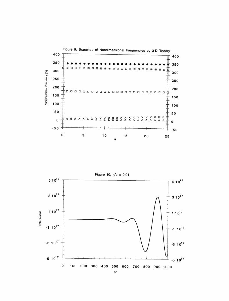
Figure 9: Branches of Nondimensional Frequencies by 3-D Theory
400
350
300
250
200
150
100
50
0
-50
252015105
• • ••• •••••••• •••••• •• •••ffi ffi ffi ffi ffi ffi ffi ffi ffi ffi ffi ffi ffi ffi ffi ffi ffi ffi ffi ffi ffi ffi ffi ffi
o 0 0 0 0 0 0 0 0 0 0 000 0 0 0 0 0 0 0 0 0 0
400
350
9- 300>-"c: 250(IJ
'"e-(IJ
It200iiic:
0"inc: 150(IJ
E'0c:0 100z
50
0
-50
0N
Figure 10: h/a = 0.01
-5 1017
o 100 200 300 400 500 600 700 800 900 1000
Q'


