To Appear in Environment and Planning B (2012)

Visualization-based Decision Tool

for Urban Meteorological Modeling

Daniel G. Aliaga1 Carlos Vanegas1 Ming Lei2 Dev Niyogi2

1 Department of Computer Science

2 Department of Earth and Atmospheric Sciences

Purdue University

Abstract—We present a visualization-based decision tool that enables exploring the link between urban land use and urban

weather, in particular predicting and visualizing changes in urban temperature, precipitation, and humidity. Our work combines

recent work from urban planning, weather and climate studies, and visualization and computer graphics. Our approach uses an

interactive tool to quickly and automatically produce plausible detailed 3D city models by means of a hybrid computational

simulation of urban behavior and procedural urban geometry. From the city model, urban morphology parameters are efficiently

computed and used by our custom meteorological simulator which considers the influence of the urban landscape. The result is

a compelling visualization ability for understanding the complex feedback between urban land use and the regional meteorology

of current cities and of potential future cities with desired greening patterns. Our work includes a case study example spanning

a 1600 km2 area.

1 Introduction

In this paper, we provid e a visualization-driven deci-

sion tool composed of automatic 3D city model genera-

tion, urban morphology calculation, and an integrated

meteorological simulation. Our work includes a case

study example for the city of Ind ianapolis with prescribed

land use change scenarios generated by our tool and the

assessment of resulting impact on regional meteorology

using a coupled numerical weather pred iction model.

1.1 Motivation Visualizing and assessing the interdependency of

dense urban development and local weather is critical to

a variety of stakeholders. Urban areas have a high pop u-

lation density and are important seats of socioeconomic

activities. Further, as a result of build ings materials and

human activities, urban areas are also typically warmer

than the surrounding areas. This Urban Heat Island (UHI)

phenomenon is well documented (Oke 1988) and has a

variety of biophysical, ecological, energy, health , and be-

havioral impacts (Brunsdon et al. 2009, Eliasson et al.

2007). Urban areas can contribute to the warming of the

regional climate (Fall et al. 2009), and thus developing

“greener” build ings is being considered as one of the cli-

mate change mitigation strategies (Akbari et al. 2009).

Several p lanning and assessment operations consider

urban structures and regional effects but are often per-

formed manually and are time consuming. For example,

several works have proposed case-specific landscape and

urban planning strategies (Shashua-Bar et al. 2009), eco-

logical concepts (Stremke and Koh 2010), and urban

greening methodologies (Bowler et al. 2010, Conway

2009) that improve urban climate and urban life quality.

1.2 Challenges Our work seeks to enable intuitively exploring “what

if” scenarios of the complex feedback occurring between

the urban space and the regional weather/ climate. Specif-

ically, we address three challenges which have not been

addressed by previous works in a cohesive and coherent

framework and consequently have limited the integration

of meteorological modeling with urban planning (Eli-

asson 2000). First, our work builds upon and extends ur-

ban modeling and simulation efforts. These systems are

typically concerned either with explicit 3D reconstruction

of an existing city from photographs or from LI-

DAR/ laser data, or with simulating the spatial d istribu-

tion of streets, population, jobs, and other demographic

data. The systems are not concerned with efficiently creat-

ing and changing 3D city models or with modeling the

effects on the regional meteorology.

Second , we improve meteorological modeling systems

by includ ing urban land surface interactions in the sim u-

lation and by automatically computing the necessary u r-

ban morphology parameters. While a few meteorological

systems support land surface models at high spatial reso-

lution (e.g., 1 to 10 kilometers) and explicitly represent the

urban land surface and the associated energy balance

(e.g., Masson 2000), in all cases the computation of the

urban morphology requires an a priori detailed 3D

knowledge of the desired (future) urban space and often

manually computes urban morphology parameters. In

contrast, we combine our 3D city model exploration tool

with automatic calculation of urban morphology values

in order to easily calculate meteorological pred ictions.

Third , while the impact of the urban landscape on re-

gional weather is well documented (Cotton et al. 2003,

Niyogi et al. 2006 and 2010, Oke 1988, Shepherd et al.

2002), visualizations have usually been limited to strictly

viewing, a posteriori, simulation data using map -based

representations and choroplethic renderings of spatially-

varying data. They do not exploit the visualization notion

that users are comfortable with viewing and understand-

ing 3D models of urban landscape and visualizations of

meteorological effects. Even without inspecting up close

To Appear in Environment and Planning B (2012)

and in detail, the overall pattern of streets, size of yards,

mixture of build ings and green spaces, and amount of

open space all contribute to provid ing an intuitive view of

a place suitable for viewers of a w ide range of expertise.

By coupling automatic generation of 3D city models with

an urban meteorological model, our tool provides a sub-

stantial step forward in build ing integrated and compel-

ling visualization (and simulation) systems for use in dy-

namic urban land use / land cover (LULC) planning, ur-

ban weather patterns, and climate change mitigation .

1.2 Overview Our visualization-based system enables assessing a

novel urban scenario by automatically creating a 3D city

model from LULC, population, and terrain elevation data ,

computing urban morphology values, and simulating the

regional meteorological behavior. The typical usage cycle

begins with an initial city model that can resemble an ex-

isting location or a desired future city. After viewing a city

model and its resulting weather patterns, the user (or de-

cision maker) can interactively alter the city model and

repeat the cycle (see Figure 1; this figure will be further

explained in the results section). Hence, urban planning

policies and weather mitigation polices can be explored .

Our urban modeling methodology for creating a 3D

city model and for computing the urban morphology p a-

rameters is to use an urban behavioral simulation process

integrated with an urban geometry procedural generation

process. This hybrid city-modeling process uses only a

coarse specification of social and economic parameters of

a city yet results in the automatic creation of a plausible

3D instantiation of the city. While the produced city mod-

el does not precisely recreate an existing urban area, it

does produce a model of sufficient qualitative similarity

to visualize the urban environment and to compute urban

morphology parameters.

Our meteorological modeling system is based on the

Regional Atmosphere Modeling System (RAMS version

4.3) (Cotton et al. 2003) coupled with an urban energy

balance model-town energy budget (TEB) (Masson 2000).

The system, together with the automatically computed

urban morphology parameters considers the role of the

urban landscape in pred icted meteorological phenomena

(e.g., storms and precipitation).

Altogether, we demonstrate our system in a case study

example of over a 1600 km2 area centered on Ind ianapolis,

IN (USA). We compare the results of a control scenario

and various “what-if” greening scenarios with the objec-

tive of visualizing and understand ing how to mitigate the

local climate by d ifferent configurations.

1.3 Impact and Contributions The impact and contributions of our work includes:

a first system to dynamically integrate urban

LULC planning and high impact/ extreme weather

mitigation into a unified framework that enables

stakeholders to explore the effects of adopting d if-

ferent urban land configurations,

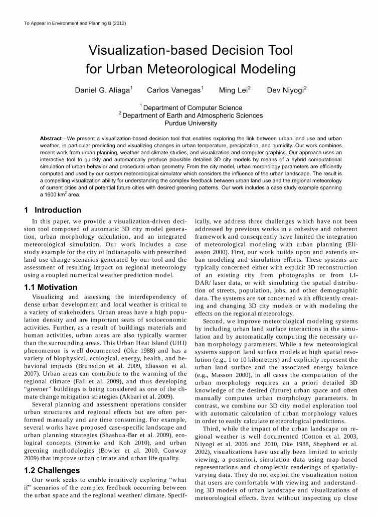
Figure 1. Visualization-based Decision Tool. Top: original urban scenario for Indianapolis, IN. Bottom: hypothetical (edited) urban sce-nario where the southwest corner became parks. Using LULC data (left column), complemented by population and terrain data, our tool automatically produces a plausible 3D city model (second and third columns) from which urban morphology parameters are extracted for a regional weather simulation over Indiana (fourth and rightmost columns). The ability to quickly edit the city model and automatically pro-duce a plausible city and urban morphology parameters offers a substantial step forward in building integrated visualization and simulation systems for use in exploring policies for urban development and urban weather mitigation. In this example, the proposed change increases city temperature and decreases city rainfall.

To Appear in Environment and Planning B (2012)

a method to generate 3D city models from land -

use, population, and terrain elevation data, and to

interactively ed it the city model assisted by an in-

tegrated urban simulation system to keep the

model within a plausible configuration, and

a set of algorithms to compute the urban mor-

phology parameters necessary for regional weath-

er simulation and visualization.

2. Related Work

Our research builds upon urban planning, simulation

and visualization, meteorological modeling, and 3D ur-

ban modeling. Urban planning is of central importance in

today’s rapid ly growing urban areas. Early works have

considered the effect of urban planning on local climate.

For example, Randall et al. (2003) proposed an extension

to ArcGIS that enables the designer to “green” d ifferent

parts of a city using one or more naturalization strategies.

Adolphe et al. (2001) suggest simplified ways to compute

ind icators of urban morphology and to d irectly use those

to plan for future urban climates. Recently, Shepherd et al.

(2010) stud ied the effect of future urban growth on local

weather for Houston, TX. However, the aforementioned

systems provide a limited , if any, closed-loop system be-

tween urban modeling and urban weather simulation,

and do not include automatic 3D urban modeling.

Urban simulation and visualization is trad itionally used

to help regional planning agencies evaluate alternative

transportation investments, land use regulations, emer-

gency response plans, and environmental protection poli-

cies (e.g., Terzi and Kaya 2011, Torrens and O’Sullivan

2001, Westervelt et al. 2011). A variety of entertainment

applications also seek to simulate and grow plausible cit-

ies for use in games and in movies. Urban simulation

models can be loosely d ivided into three dominant para-

d igms: cellular automata methods (Clark and Gaydos

1998, Al-kheder et al. 2008), agent-based methods (Portu-

gali 2000), and urban-economic d iscrete choice models

(De Palma et al. 2007, Vanegas et al. 2009a). Urban visual-

ization often makes use of techniques includ ing chorople-

thic maps generated by exporting simulation results,

summarized by a zonal geography, to a GIS for rendering

(e.g., Schwartzman and Borning 2007). Urban simulation

and visualization does not typically address creating a 3D

city nor does it focus on generating parameters for a m e-

teorological simulation. Nevertheless, studies have shown

that visualization helps in d isseminating and commun i-

cating the results of a planning or simulation scenario

(Laing et al. 2009, Pettit et al. 2011). Moreover, the im-

proved communication can foment the adoption of env i-

ronmentally-friend ly planning (Brody et al. 2008).

Meteorological simulations that explicitly consider the ef-

fects of urban landscape are significantly d ifferent from

simulations over other natural LULC. This is primarily

due to the unique physical property of artificial materials

and has d rawn increased research interest in recent years

(Akbari et al. 2009, McCarthy et al. 2010, Masson 2000,

Oleson et al. 2010). The Urban Heat Island is caused by

the high heat capacity and low albedo of concrete build -

ings. Tall build ings also lead to the higher roughness and

d isplacement length that alters regional su rface winds

and the atmospheric boundary layer conver-

gence/ d ivergence patterns. Moreover, urban landscape

generally has lower evaporation/ transpiration or latent

heat flux as compared to the surrounding rural region.

This creates spatial grad ients in surface heat fluxes, which

combined with changes in boundary layer convergence

can create zones of preferential convection, and mesoscale

weather patterns and climatic regimes (Niyogi et al. 2010).

Most urban weather simulation methods assume either a

very simple urban geometrical model or offload all mod-

eling to time consuming manual efforts (Niyogi et al.

2006).

3D urban modeling methods have been proposed to cre-

ate detailed geometric models of cities and of build ings.

Parish and Mueller ’s (2001) pioneering method created

city models using a grammar-based approach. Such an

approach has been extended to the generation of build -

ings and road networks (e.g., Aliaga et al. 2008, Chen et

al. 2008, Lipp et al. 2008). However, none of these efforts

have investigated effects on regional meteorology.

Recently, several research works have proposed an in-

terd isciplinary collaboration between visualization and

urban-related simulations to produce new modeling

techniques. These techniques facilitate an intuitive

presentation and increase the impact of urban simulation

to many stakeholders. For example, Weber et al. (2009)

describe a geometrical simulation system that models the

plausible growth of a 3D urban model over time, based

on an exogenous population model. Vanegas et al. (2009a)

provide a visualization system that uses the output of a

temporal agent-based urban simulation to make plausible

images of future road and parcel networks. Vanegas et al.

2009b merge behavioral and geometrical modeling of u r-

ban areas in order to reduce the design time of 3D city

models. However, in these works the focus is on design-

ing and ed iting a new urban model, and not on modeling

or assessing the meteorological impact of a current or a l-

tered city. Therefore, these systems do not produce any

ind icators for climatic patterns, do not support creating

Figure 2. System Pipeline. A summary of our system pipeline. Given LULC, population, and terrain elevation data, we create an initial city model. Using the city model, we compute urban morphology parameters and new LULC/population data (if appli-cable). The results are fed to our urban weather simulation and then visualized by the user. The user can then perform high-level editing operations on the model and repeat the cycle.

To Appear in Environment and Planning B (2012)

3D models from LULC database, and do not provide cu s-

tomized tools for interactive ed iting of behavioral and

geometric variables that affect meteorological processes,

as is undertaken in the present study.

3. Urban Weather Decision Tool

Our system enables cycling through the process of cre-

ating/ ed iting a 3D city model, automatically generating

parameter values for a meteorological simulation and

then simulating urban weather over a short time horizon

(e.g., a few days). Figure 2 provides an outline of our

computational pipeline. The initial city model is created

using LULC data, population/ jobs data (e.g., census in-

formation), and terrain elevation data. Our system then

computes urban morphology param eter values suitable

for our urban weather simulation. The resulting simula-

tion values and city model are visualized by the user (e.g.,

3D renderings, choroplethic maps, etc.). The user can then

interactively change the city model using high-level ed it-

ing tools. New urban morphology parameter values are

computed and the cycle repeats enabling the exploration

and visualization of new city designs and the resulting

urban weather.

To support the various high-level city editing opera-

tions, we enable easy alteration of the LULC, popula-

tion/ jobs, terrain, and other input values. When explor-

ing alternative city designs, we are interested in large

scale policy-relevant changes such as “greening the city”,

“placing parks throughout the city”, “enforcing popula-

tion/ housing growth into certain areas”, and “altering the

shape of the urban contour with the surrounding non -

urban land”. Meanwhile, our automatic city model gen-

eration ensures a su fficiently accurate and plausible 3D

model is created for use in the weather simulation.

Our ed iting interface uses a paint-brush style tool to

alter the aforementioned input values. For example, to

green a zone, the user selects the “greening” brush and

clicks on the area where greening should occur. The rad i-

us and intensity of the brush can be controlled to deter-

mine, in this particular case, the area of the greening zone

and the density of the greening. This operation corre-

sponds to setting the grid cells inside the brush to vegeta-

tion-covered locations. Similarly, terrain ed iting implies

varying the elevation of the terrain and , in some cases,

ind icating the affected grid cells are covered by water

bodies. Population relocation corresponds to moving d e-

veloped zones covered with urban infrastructure.

4. Urban Geometry and Morphology

In the following, we describe how a geometrical mod-

el of a target city is efficiently generated and how urban

morphology parameter values are estimated from the

automatically produced city model.

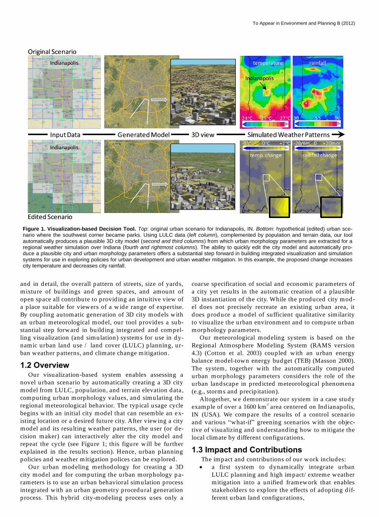
4.1. Geometry Generation Our generation process creates a 3D city model that

resembles a chosen city and is suitable for urban mor-

phology estimation (Figure 3). While airborne and terres-

trial scanned cities are available, obtaining such scans is a

very large effort. Moreover, the resulting models usually

consist of a large collection of unstructured polygons.

Hence, although the models contain more geometric de-

tails than needed for an urban weather simulation (i.e.,

the canyon model), there is no relation to the underlying

urban attribute layers. This hinders their use in urban

weather simulations and in high-level model ed iting. In-

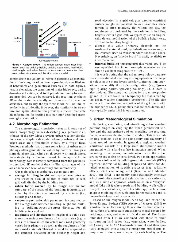
Figure 3. Canyon Model. The urban canyon model uses infor-mation such as building height, building separation, road width, road length, and other factors to estimate the interaction be-tween urban structures and the atmospheric model.

Figure 3. Urban Geometry Generation. On the left, we show LULC, population, and terrain specification (e.g., elevation, parks, water bodies) used to generate a plausible 3D city model. On the right, we compare the generated synthetic model to an actual map of Indian-apolis (from Google Maps). Our system generates geometry that although not identical to the actual city is qualitatively similar. Note: since highways are not generated by a very predictable and/or understood process, we specify highways by hand.

To Appear in Environment and Planning B (2012)

stead , we seek to require only a relatively sparse amount

of input and to support using our system in a large nu m-

ber of cities, even if a 3D scan is not available.

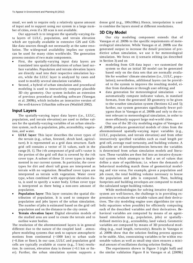
Our approach is to integrate the spatially-varying da-

ta layers of LULC, population, and terrain elevation

which are typically available in extensive GIS and GIS-

like data sources though not necessarily at the same reso-

lution. The widespread availability implies our system

can be used for many cities worldwide. The generation

process consists of two main components.

First, the spatially-varying input data layers are

translated into spatial d istributions of urban land sur-

face variables. Population and terrain elevation layers

are d irectly read into their respective simulation lay-

ers, while the LULC layer is analyzed by cases and

used to modify several simulation variables.

Second , a hybrid of urban simulation and procedural

modeling is used to interactively compute plausible

3D city geometry. Our system includes an extension

of previous procedural modeling software (Vanegas

et al. 2009b), which includes an interactive version of

the well-known UrbanSim software (Waddell 2002).

Input Layers The spatially-varying input data layers (i.e., LULC,

population, and terrain elevation) are used to define val-

ues for the spatially-varying variables of an urban simula-

tion system, such as population, jobs, accessibility, vegeta-

tion, and water.

LULC layer: This layer describes the cover types of

the terrain (e.g., urban, forested , shrub land , agricu l-

ture). It is represented as a grid data structure. Each

grid cell contains a vector of 31 values, each in the

range [0, 1]. The i-th component of grid cell’s vector is

the portion of the grid cell that is covered by the i-th

cover type. A subset of these 31 cover types is imple-

mented in our current system. In particular, the cover

types for d irt and short/ tall grass are interpreted as

terrain with no vegetation. Broad leaf cover types are

interpreted as terrain with vegetation. Water cover

type, when combined with appropriate elevation da-

ta, is used to specify a water body. Urban cover type

is interpreted as there being a non-zero amount of

population.

Population layer: This layer contains the spatial d is-

tribution of population . It is used to compute the

population and jobs layers of the urban simulation.

The number of jobs is estimated based on the grid cell

population and on the d istance to the city center.

Terrain elevation layer: Digital elevation models of

the stud ied area are used to create the terrain and to

outline water bodies.

The resolution of the aforementioned layers is in general

d ifferent due to the nature of the coupled land – atmos-

phere modeling systems that seek to capture atmospheric

motions from continental (~1000 km) to urban scale

(~0.1km or finer). In our case, LULC and population grid

cells are typically available at coarse (e.g., 5 km) resolu-

tion. In contrast, elevation data is denser (~0.1 km or fin-

er). Further, the urban simulation system supports a

dense grid (e.g., 100x100m). Hence, interpolation is used

to combine the layers stored at d ifferent resolutions.

3D City Model Our city modeling component extends that of

Vanegas et al. 2009b to the specific requirements of mete-

orological simulation. While Vanegas et al. 2009b use the

generated output to increase the detail/ precision of pre-

d ictive urban simulation, we use it for meteorological

simulation. We focus on i) scenario ed iting (as described

in Section 3) and on

modeling from GIS data input - we customized the

system so that an initial 3D model can be generated

based only on the data sets that are normally availa-

ble for weather/ climate simulation (i.e., LULC, pop u-

lation); nevertheless, add itional layers can be provid-

ed to the system to improve the resulting model, ei-

ther from databases or through user ed it ing; and

data generation for meteorological simulation – we

automatically compute ind icator values, in standard

formats, from the generated 3D geometry to be given

to the weather simulation system (Sections 4.2 and 5);

further, our system generates significantly fewer pol-

ygons than in Vanegas et al. 2009b and only to the ex-

tent relevant to meteorological simulation, in order to

more efficiently support large real-world cities.

Our use of the 3D city modeling engine of Vanegas et

al. 2009b produces geometrical models of cities from the

aforementioned spatially-varying input variables (e.g.,

LULC, population, and terrain elevation) and from other

interactively specified variables such as road length per

grid cell, average road tortuosity, and build ing volume. A

plausible set of interdependencies between the variables

is determined from urban simulation models and litera-

ture. These variables are then fed into an iterative dynam-

ical system which attempts to find a set of values that

define a state of equilibrium; i.e. where the demands of

behavioral modeling match those of geometrical model-

ing and vice versa. For example, given a population and

job count, the total build ing volume necessary to house

the population and jobs is computed . Then, build ing

footprints and build ing envelopes are computed to match

the calculated target build ing volume.

While methodologies for solving iterative dynamical

system are well-known, the challenge is in provid ing ex-

pressions to evaluate the variable values and their deriv a-

tives. The city modeling engine uses algorithms (or sym-

bolic equations when possible) for efficiently computing

each of the described variables and their derivatives. Be-

havioral variables are computed by means of an agent-

based simulation (e.g., population, jobs) or spatially -

defined metrics (e.g., accessibility, land value). Geometric

variables are computed by means of 3D procedural mod-

eling (e.g., road length, tortuosity). Results in Vanegas et

al. 2009b show that the solution find ing process appears

to be stable. Also, constraining variables to be within rea-

sonable values as well as small step sizes ensures a min i-

mal amount of oscillations during solution find ing.

The experiments shown in Figure 3 (right half) and

the similar validation Figure 8 in Vanegas et al. [2009b]

To Appear in Environment and Planning B (2012)

demonstrate the ability to recreate plausible approxim a-

tions of existing locations from a previously specified set

of behavioral and geometrical variables. In both figures,

terrain elevation, the centerline of major highways, parks,

downtown location, and total population and jobs count

are provided . As can be observed , the resulting synthetic

3D model is similar visually and in terms of substantive

attributes, but clearly, the synthetic model will not match

perfectly in all details. However, the similarity in stru c-

ture and spatial d istribution provides sufficient plausible

3D information for feed ing into our later described mete-

orological simulation.

4.2. Morphology Estimation The meteorological simulation takes as input a set of

urban morphology values describing key geometric at-

tributes of the city. Most previous urban weather simula-

tions use a simple slab model whereby urban and non -

urban areas are d ifferentiated merely by a “type” field .

Previous methods that do use some form of urban mor-

phology often generate the values by hand or through a

static database (e.g., Ching et al. 2009), with much effort,

for a single city or fraction thereof. In our approach, the

morphology data is d irectly computed from the previous-

ly described 3D model of the city. The advantages of this

are an increased level of accuracy and automaticity.

Our main urban morphology parameters are:

average building height: our system computes an

area-weighted sum of heights of build ings in each

grid cell, d ivided by the build ing count.

urban fabric covered by buildings: our method

sums up of the areas of the build ing footprints, d i-

vided by the total area covered by structures (i.e.,

build ings and roads).

canyon aspect ratio: this parameter is computed as

the average ratio between build ing height and build -

ing to build ing-across-the-street d istance, for all

build ings in a grid cell.

roughness and displacement length: this value esti-

mates the surface roughness of an urban area (e.g., a

measure of how much the actual roof/ road geometry

varies from planarity as well as the roughness of the

roof/ road material). This value could be computed as

the standard deviation of the build ings height and

road elevation in a grid cell plus another empirical

surface roughness constant. In our examples, since

terrain is often relatively flat within the city, the

roughness is dominated by the variation in build ing

heights within a grid cell. We typically use an empir i-

cally determined fraction of the build ing height (e.g.,

1/ 10 of the build ing height).

albedo: this value primarily depends on the

road / roof material used ; by default we use an empir-

ical constant used to mimic standard roads and roofs.

Nevertheless, an "albedo brush" is easily available to

alter the value.

internal building temperature: this value could be

user-specified but in our example scenario we as-

sume a constant temperature of 17ºC.

It is worth noting that the urban morphology param e-

ters are re-estimated after any ed iting operation or change

of values in the input layers. Similarly, after ed iting oper-

ations that modify the city’s configuration (e.g., "green-

ing", "placing parks", "growing housing"), LULC data is

also updated . The computed values for urban morpholo-

gy and LULC are saved in a temporary file that is read by

the urban weather simulation component. The file size

varies with the size and resolution of the grid , and with

the number of LULC parameters that are considered , and

was typically under 1MB in ou r examples.

5. Urban Meteorological Simulation

Exploring, simulating, and visualizing urban weather

patterns hinges on coupling the urban geometrical su r-

face and the atmosphere and on modeling the resulting

fluxes in meso-scale atmospheric models. This is a chal-

lenging problem due to the complexity and d iversity of

cities around the world . In general, a regional weather

simulation consists of a large-scale atmospheric model

integrated with a land -surface interaction model. When

includ ing urban areas, the in teraction with the urban

structures must also be considered . Two main approaches

have been followed: i) build ing-resolving models (BRM)

represent ind ividual build ing shapes and allow for d e-

tailed examination of specific processes (e.g., rad iative

effects, wind channeling, etc.) (Teemusk and Mander

2010), but BRM is inherently computationally-intensive

which prohibits extend ing the simulation to an entire city,

and ii) a simpler approach which relies on a “canyon”

model (Oke 1988) where roads and build ing walls collec-

tively form a set of canyons. This latter approach is more

adept at modeling cities with large horizontal sizes and is

the methodology used in our work.

Based on the canyon model, we adapt and extend the

Town Energy Budget (TEB) scheme of Masson (2000) to

simulate the surface energy fluxes into the atmosphere at

the surface of a mesoscale atmospheric model covered by

build ings, roads, and other artificial material. The fluxes

estimated from TEB are combined with those of other

surrounding land types (e.g., vegetation, water bodies,

etc.) using the LEAF2 land -surface model and then spa-

tially averaged into a single atmospheric model grid in

proportion to the space occupied by each land type. The

Figure 4. Canyon Model. The urban canyon model uses infor-mation such as building height, building separation, road width, road length, and other factors to estimate the interaction be-tween urban structures and the atmospheric model.

To Appear in Environment and Planning B (2012)

overall atmospheric simulation system we use is the

RAMS version 4.3 (Cotton et al. 2003). RAMS is a well-

tested multi-scale environmental modeling system, and

has been applied to a wide range of problems (e.g. flow

around build ings, thunderstorm dynamics, regional cir-

culations, and continental scale climate change analysis).

Our implementation addresses the challenge of inte-

gration of fine scale data, needed to accurately represent

the urban landscape morphology, and coarser scale com-

putational and theoretical requirements of the formula-

tions used within numerical weather pred iction (NVP)

models (i.e., RAMS). For instance, urban morphology

expects 1 m resolution while the NWP model grid spacing

is typically around 1 km. To blend these heterogeneous

scales, a possible approach -- and the one adopted in this

study -- is to use a subgrid scale representation of the

landscape ‘tiles’ within the larger grid . The patchwork of

d ifferent land uses within a model grid are aggregated to

form a single ‘tile’. The four most prominent landscapes

in a grid (i.e., from a choice of International Geosphere-

Biosphere Programme land use categories such as mixed

forest, shrublands, mixed agriculture, deciduous forest,

urban, etc.), and the urban region (if not already part of

the top four land use fraction in that grid ) are tiled to-

gether to form the grid -based landuse representation. The

model equations for energy and hydrological balance are

then solved for each tile and then area-weighed to devel-

op the grid averaged value. Following Avissar and Pielke

(1989), a subgrid scale flux correction is also made to ac-

count for the tiling heterogeneity.

Specific within the LEAF2 urban tile, the leaf area in-

dex and fractional vegetation coverage are decreased

while the aerodynamic roughness length is increased to

approximate hydrodynamic effects. In coupling with TEB,

the generalized canyon model replaces the LEAF2 urban

class parameterization to better represent the urban pro-

cesses. The 3D urban surface and roughness sub-layer

interactions required for solving the surface layer feed-

backs in the mesoscale model and the input data for TEB

is imported from the 3D visualization model. TEB pro-

vides the lower boundary conditions required for the a t-

mospheric model to respond to and the simulated fore-

cast for surface quantities includ ing sensible hea t flux,

latent heat flux, momentum changes, albedo, and emis-

sivity. RAMS imported TEB’s fluxes for each grid cell at

the first atmospheric level as an urban patch contribution,

then average with LEAF2 nonurban patches are transla t-

ed into soil moisture/ temp erature changes, and air tem-

perature, humid ity and winds following surface layer

similarity approaches (Arya 1988). The total (grid aver-

aged) fluxes and scalar output for the grid cells with u r-

ban land use consist of both TEB and LEAF2 values.

Figure 4 depicts the geometrical configuration used by

the TEB. The main shape d imensions include values for

road length, road wid th, build ing separation, and build -

ing height. The TEB uses and computes three surfaces

temperatures: one for each of roofs, roads, and walls. For

each surface type, one or more layers are present – this

enables modeling the fluxes to/ from build ing interiors

(e.g., walls and roofs) or to/ from the ground (e.g., roads).

Further, since surface temperatures are included in the

model, it is possible to model the evaporation of water

accumulated from precipitation. The TEB assumes surfac-

es to be impervious and lets water evaporate as long as

the air humid ity is unsaturated and there is still water on

the surfaces. In add ition, the TEB accounts for solar rad ia-

tion trapped inside the urban structures by considering

how much of the sky is visible from the walls/ streets

(roofs always have full view of the sky). Finally, the TEB

also considers anthropogenic fluxes (i.e., fluxes due to

human activity) which primarily consist of domestic heat-

ing and combustion.

6. Implementation Details

Our geometry generation system, urban morphology

estimation, and model ed iting tools run on a desktop PC

with a 3.0GHz processor and 4GB memory. Our urban

modeling system is an extension of the infrastructure d e-

scribed in Vanegas et al. 2009b (available upon request

from authors). All rendering is done on the PC using an

NVid ia Quadro FX 1700 graphics card . The compute time

for city generation and for all visualizations ranges from

seconds to minutes.

The regional weather simulation is based on the RAMS

system [Cotton et al. 2003] (available at http:/ /

bridge.atmet.org/ users/ software.php , version 4.3). The

simulator runs on a cluster using up to 5120 cores (640

nodes of 32GB memory, each node with 8 2.5 GHz cores,

and interconnected by 10 gigabit Ethernet). The cluster-

and PC-based portions of our system communicate using

temporary files. The offline simulation compute time de-

pends on the total region size and the grid sizes of the

simulated area; i.e., time-accuracy tradeoffs can be made.

In our experiments, we need 6 to 24 hours for a simulated

time of 3 days depending on the grid resolution, process

calculations and representations, and system efficiency.

Our example case-study focuses on the Ind ianapolis,

IN, USA metropolitan area. This area spans approxim ate-

ly 50 by 45 kilometers and has nearly two million people.

To make the simulation practical on our cluster, our high-

est level-of-detail regional weather simulation was con-

figured with three telescopic nested grids with 80, 20, and

5 km grid spacing with a common center point at 39.77N

and 86.16W (i.e., downtown Ind ianapolis). Grid 1 had 64

x 48 horizontal grid points covering the ent ire continental

United States (US) with a prognostic time step of 90 se-

conds. The second grid had 82 x 74 horizontal grid points

covering most of the Eastern part of the US with a time

step of 30 seconds. The third grid comprised of 94 x 94

horizontal grid points with a time step of 10 seconds, and

covers all of Ind iana. The model was configured based on

success with previous cases documented in Lei et al.

(2008) and Lei and Niyogi (2011) and with terrain follow-

ing the pressure/ sigma-coord inate system with 36 verti-

cal layers with a finer vertical spacing from 0.05 km to

1.27 km and a fixed spacing thereafter until 8.5 km, and a

total depth of the model atmosphere set to 21 km. The

TEB was coupled only over the inner most region of grid

3 which covers the Ind ianapolis urban area. Urban energy

To Appear in Environment and Planning B (2012)

balance was invoked on the grid either with TEB (for grid

3) or a simpler slab model for the outer two domains.

The input layer data was obtained from county and

GIS databases: LULC data came from U.S. Geological

Survey and the population data is from year 2000 census.

The simulation model was initialized using NOAA Final

Analysis (FNL) data, which were also used for provid ing

the lateral boundary conditions every 12 hours for the

outermost domain.

For add itional information about system details

and / or copy of the datasets, please contact the authors.

7. Example Results

In this section, we explore several altered urban sce-

narios of the region surrounding Ind ianapolis, IN with

d ifferent greening configurations. Recent investigations

have shown that varying the green areas (Clark et al.

2010, Conway 2009, DeNardo et al. 2005, Oberndorfer et

al. 2007) and the geometry and material of urban area

build ings (Teemusk and Mander 2010) can significantly

alter temperature, humid ity, and rainfall, for example.

Using our system, decision makers can view and explore

tentative city models as well as choroplethic maps of the

weather. In our examples and during the simulation time

Figure 5. Visualizations of Urban Weather Mitigation. Visualization of greening the NW (top row), NE (middle row), or SE (bottom row) corner of Indianapolis. The first column shows a map-style view of the automatically generated 3D model produced by our system. The second, third, and fourth columns show the change in temperature, humidity, and rainfall as compared to the control scenario. Close-ups are provided of the temperature change over Indianapolis.

Temperature Change Humidity Change Rainfall Change

NW greening

NE greening

Urban Scenario

SE greening

-1C 0C +1C -5% 0% +5% +20mm

-0.7C +0.3C

-20mm 0

Indianapolis

To Appear in Environment and Planning B (2012)

frame, the surrounding regional weather (e.g., from state

and country level meteorological phenomena) is produc-

ing southwest winds over Ind ianapolis (e.g., winds from

the southwest and to the northeast). A region that receives

the winds first is said to be “upwind” and region that

receives it second (or later) is called “downwind”. As a

control simulation, we perform a 3-day urban weather

simulation over the current configuration of Ind ianapolis.

The base-levels of temperature, rainfall, and humid ity of

this control scenario are shown in the two upper-

rightmost images of Figure 1 and in the left-most image in

Figure 7.

A first explorative scenario is to add parks over the

southwest (SW) corner of Ind ianapolis (Figure 1). The SW

corner is upwind and hence is the first part of the metro-

politan area hit by incoming regional weather activity

(e.g., by a thunderstorm) from the larger surrounding

area. To create this scenario (and all other scenarios), we

use our interactive system to perform a high -level green-

ing operation by changing the LULC for the selected re-

gion to parks using our GUI and then the system auto-

matically red istributes the affected population to else-

where in the city and generates a plausible new set of

streets and build ing structures.

Figure 1 shows views of the generated 3D city and col-

ored imagery of the simulation results. These results

show the expected temperature decrease over the SW

corner. Research stud ies of partial greening (e.g., near

50% greening of roof tops in New York City (Rosenzweig

et al. 2006), similar greening in subsets of Toronto, Ontar-

io (Banting et al. 2005), add ition of parks as stud ied by

Bowler et al. (2010)) has showed temperature reductions

of 0.8°C to 2°C, which are similar in range to our results.

However, due to the feedback on other weather variables

almost all other areas over downwind Ind ianapolis be-

come warmer in this case. In add ition, there is less rainfall

over Ind ianapolis but noticeably more rainfall further

downwind from Ind ianapolis (i.e., over the NE corner

outside of Ind ianapolis). It has been observed that the

cooling effects of green areas within a city can affect

weather far beyond the boundary of the green area itself

(Honjo and Takakura 1991). Thus, in general green areas

have lower temperatures and higher humid ity as com-

pared to dense urban (cement) areas. But the weather re-

sulting from large green areas can affect not only other

parts in the city but also surrounding non-urban areas

(Lei and Niyogi 2011). Hence, the tempera-

ture/ humid ity/ rainfall changes that are observed are

typical of regional meteorological simulations and are not

model artifacts. Our system assists in pred icting the gen-

eral tendencies that are most likely under the provided

initial conditions (Shepherd et al. 2010). In summary, our

first scenario increases the average city temperature, de-

creases rainfall over Ind ianapolis, and increases rainfall

over the NE corner outside of Ind ianapolis.

In this second experiment, we add some parks over the

northwest (NW) corner of Ind ianapolis (Figure 5, top-

row). Similar to the first experiment, the temperature d e-

-20 0

Circular Greening

Distributed Greening

-1C 0C 1C

Indianapolis

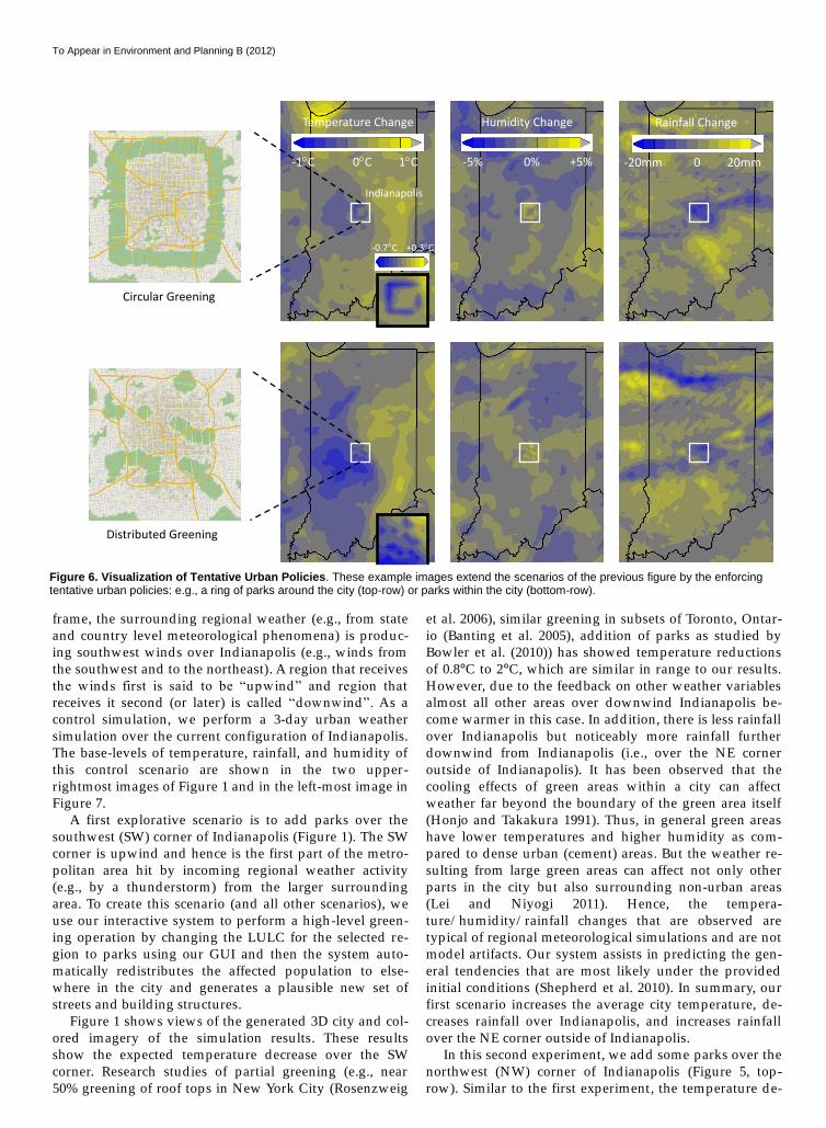
Figure 6. Visualization of Tentative Urban Policies. These example images extend the scenarios of the previous figure by the enforcing tentative urban policies: e.g., a ring of parks around the city (top-row) or parks within the city (bottom-row).

Temperature Change Humidity Change Rainfall Change

-0.7C +0.3C

-5% 0% +5% -20mm 20mm 0

To Appear in Environment and Planning B (2012)

creases and humid ity increases over the NW corner. But

in this scenario, the average temperature over Ind ianap o-

lis increases less than in the first scenario, the rainfall over

Ind ianapolis is even less than in the first scenario, and

almost no increase of rainfall occurs over the NE corner

outside of Ind ianapolis. Given an objective of d iscovering

a city configuration with no significant average tempera-

ture change and less rainfall, this scenario is a suitable

one.

In a third and fourth experiment, we add some parks

either over the northeast (NE) corner (Figure 5, middle

row) or of the southeast (SE) corner (Figure 5, bottom

row) of Ind ianapolis. In both of these scenarios, we ob-

serve both the temperature and the rainfall over Ind ian-

apolis generally decrease. Moreover, for the greening of

the SE corner the temperature decreases the most while

for the greening of the NE corner the least overall rainfall

is produced , especially in the upper north half of the city.

Thus, if the desire is to decrease temperature and rainfall

over Ind ianapolis, these configurations provide options

with d ifferent tradeoffs. The SE greening option provides

the largest temperature decrease (of about 1°C) because of

a successful use of greening combined with the wind pat-

tern. It is worth nothing that for a more drastic tempera-

ture reduction, it has been shown that more extensive

greening of the urban canyon (Alexandri and Jones 2008)

can have peak temperature reductions nearing 8.4°C. In-

deed for each of these options, longer term simulations

(e.g., seasonal to multi-year) will need to be performed

and the current examples are simply for illustrative pu r-

poses.

In Figure 6, we provide two additional urban scenar i-

os. These are similar to those of the Figure 5 but could be

viewed as the result of adopting an urban development

policy. Figure 6-top ensures the city is surrounded by

parks, while Figure 6-bottom enforces a policy of placing

large parks d istributed within the city. Both of these ur-

ban scenarios actually yield the most reduction in rainfall,

as compared to the examples in Figure 5, as well as a mild

temperature reduction on average. On the one hand, the

introduction of parks throughout the city reduces the

temperature the most. On the other hand , the ring of su r-

rounding parks, decreases rainfall the most.

Finally, Figure 7 succinctly visualizes the change in

humid ity as a consequence of the d ifferent greening sce-

narios. The humid ity increase over the parks is clear in

most cases. The overall behavior of humid ity can a lso be

observed . This visualization could be complemented by

views of the underlying 3D city model. Collectively, this

yields an intuitive view of several “what-if scenarios” that

would otherwise require significant manual (modeling

and estimation) effort for our ensemble of experiments.

This increase in humid ity in response to greening is an

important feature, which needs to be considered , for ex-

ample, if the aim is to reduce thermal heat stress. A small

reduction in temperature but large increase in humid ity

may actually significantly increase the heat/ thermal

stress, and cause more d iscomfort or bio-meteorological

impacts (Kalkstein 2000).

8. Discussion and Future Work

We have introduced a first system that integrates au-

tomatic urban model generation and weather simulation

into a single visualization system for exploring urban

weather mitigation. Our work is important to visualiza-

tion for it shows how tightly integrating intuitive visuali-

zations and complex simulations into a closed loop can

benefit the end-users. Our work is important to the appli-

cation domain (e.g., urban planning, regional meteorolo-

gy, and urban climate change mitigation) for it enables

quickly exploring interactions between cities and weather,

potentially lead ing to improved schemes for urban

weather modeling. Finally, our work is important to u r-

ban planning stakeholders, for it provides them with a

compelling tool to explore the effect of d ifferent urban

and regional LULC policies. While in our current system

we focus on “greening effects”, there is in principle no

limitation on the type of changes to the urban environ-

ment. Our system is not intended to choose the best urban

policies to accomplish a specified goal but is setup to en a-

ble their exploration.

With regards to future work, there are several items we

wish to pursue. First, we would like to extend the number

of urban morphology parameters and land use types that

are explicitly supported . We will also test the approach

over d ifferent urban geometries, and climate regimes (e.g.

Atlanta, Houston, Mumbai/ Ind ia, etc.). Second , aside

from a pure exploratory objective, we would also like to

enable the system to automatically search for the least

change to a current city that best accomplishes a desired

goal; e.g., seek for an urban configuration producing low-

est temperature and humid ity, or producing most rainfall

surround the city (where farmland is assumed to be).

Third , we are investigating PC-based and GPU-based

implementations of an approximate regional atmospheric

SW NE SE Ring Distributed NW

Figure 7. Example Comparison. A visualization of the effect on humidity over Indianapolis for the different scenarios. (left) The original humidity level. Each picture to the right is the relative humidity level to the original scenario for the greening scenarios of { SW, NW, NE, SE, ring, distributed } parks. SW-scenario produces the least overall humidity and SE-scenario the most overall humidity.

Original Humidity

83% -5% 78% +5%

To Appear in Environment and Planning B (2012)

modeling system to enable interactive simulation as well.

Fourth, working with the State Climate Offices, we are

actively seeking experimental deployments of our system.

9. Acknowledgments

We are grateful to our sponsors who enabled this

work includ ing NSF IIS 0964302, NSF OCI 0753116, and a

Google Research gift.

References

[1] Adolphe L., 2001. A simplified model of urban morphology:

application to an analysis of the environmental performance of

cities. Environment and Planning B, 28, 183 – 200.

[2] Akbari H., Menon S., Rosenfeld A., 2009. Global cooling: in-

creasing world-wide urban albedos to offset CO2. Climatic

Change, 94, 275-286, DOI: 10.1007/s10584-008-9515-9. [3] Al-kheder S., Wang J., and Shan J., 2008. Fuzzy inference guid-

ed cellular automata urban-growth modeling using multi-

temporal satellite images. International Journal of Geographic In-

formation Science, 22, 11-12, 1271–1293.

[4] Alexandri E. and Jones P., 2008. Temperature decreases in an

urban canyon due to green walls and green roofs in d iverse

climates. Building and Environment, Part Special: Build ing Per-

formance Simulation, 43(4), 480-493.

[5] Aliaga D. G., Vanegas C. A., and Benes B, 2008. Interactive

example-based urban layout synthesis. ACM Transactions on

Graphics 27, 5, 1–10.

[6] Arya, S.P., 1988. Introduction to micrometeorology, Academic

Press, Inc. (International Geophysics Series, Volume 42), 324 p.

[7] Avissar, R. and Pielke, Sr., R. A., 1989. A parameterization of

heterogeneous land surfaces for atmospheric numerical models

and its impact on regional meteorology. Monthly Weather Re-

view, 117, 2113–2136.

[8] Banting D., Doshi H., Li J., Missios P., Au A., Currie B.A. and

Verrati M., 2005. Report on Environmental Benefits and Costs

of Green Roof Technology for the City of Toronto. The City of

Toronto and Ontario Centres of Excellence – Earth and Environmen-

tal Technologies (OCE-ETech).

[9] Bowler D., Buyung-Ali L., Knight T., Pullin A., 2010. Urban

greening to cool towns and cities: A systematic review of the

empirical evidence. Landscape and Urban Planning, 97(3), 147-

155.

[10] Brody S., Zahran S., Grover H., Vedlitz A., 2008. A spatial anal-

ysis of local climate change policy in the United States: Risk,

stress, and opportunity. Landscape and Urban Planning, 87(1), 33-

41.

[11] Brunsdon C., Corcoran J., Higgs G., Ware A., 2009. The influ-

ence of weather on local geographical patterns of police calls for

service. Environment and Planning B, 36, 906 – 926. [12] Ching, J., M. Brown, S. Burian, F. Chen, R. Cionco, A. Hanna, T.

Hultgren, T. McPherson, D. Sailor, H. Taha, and D. Williams,

2009. National Urban Database and Access Portal Tool. Bulletin

of the American Meteorological Society, 90, 1157–1168.

[13] Chen G., Esch G., Wonka P., Mueller P., and Zhang E., 2008.

Interactive procedural street modeling. ACM Transactions on

Graphics 27, 3, 1–10.

[14] Clark C., Busiek B.E., and Adriaens P, 2010. Quantifying Ther-

mal Impacts of Green Infrastructure: Review and Gaps. Water

Environment Foundation (WEF) 2010 Cities of the Future/Urban

River Restoration Conference, Cambridge, MA.

[15] Clarke K. C., and Gaydos L.J., 1998. Loose-coupling a cellular

au tomaton model and GIS: long-term urban growth prediction

for San Francisco and Washington/ Baltimore. International

Journal of Geographical Information Science, 12(7), 699–714.

[16] Conway T., 2009. Local environmental impacts of alternative

forms of residential development. Environment and Planning B,

36, 927 – 943. [17] Cotton, W. R., Pielke, Sr., R. A., Walko, R. L., Liston, G. E.,

Tremback, C. J., Jiang, H., McAnelly, R. L., Harrington, J. Y.,

Nicholls, M. E., Carrio, G. G., and McFadden, J. P., 2003. RAMS

2001: Current Status and Future Directions. Meteorology and At-

mospherical Physics, 82, 5–29.

[18] De Palma A., Picard N., and Waddell P., 2007. Discrete choice

models with capacity constraints: An empirical analysis of the

housing market of the greater Paris region. Journal of Urban

Economics, 62, 2, 204–230.

[19] DeNardo J.C., Jarrett A.R., Manbeck H.B., Beattie D.J., and

Berghage R.D., 2005. Stormwater mitigation and surface tem-

perature reduction by green roofs. Transactions of the ASABE,

48(4), 1491-1496.

[20] Eliasson I., 2000. The use of climate knowledge in urban plan-

ning. Landscape and Urban Planning, 48(1-2), 31-44.

[21] Eliasson I., Knez I., Westerberg U., Thorsson S., Lindberg F.,

2007. Climate and behaviour in a Nordic city. Landscape and Ur-

ban Planning, 82(1-2), 72-84.

[22] Fall S., Niyogi D., Pielke Sr. R. A., Gluhovsky A., Kalnay E., and

Rochon G., 2009. Impacts of land use land cover on temperature

trends over the continental United States: assessment using the

North American Regional Reanalysis. International Journal of

Climatology, DOI: 10.1002/joc.1996. [23] Honjo T. and Takakura T., 1990-91. Simulation of Thermal Ef-

fects of Urban Green Areas on their Surrounding Areas. Energy

and Buildings, 15–16, 443.

[24] Kalkstein L., 2000. Saving lives during extreme weather in

summer, British Medical Journal, 321 : 650.

[25] Laing R., Davies A.M., Miller D., Conniff A., Scott S., Morrice J.,

2009. The application of visual environmental economics in the

study of public preference and urban greenspace. Environment

and Planning B, 36, 355 – 375. [26] Lei M., Niyogi D., Kishtawal C., Pielke Sr. R., Beltran-Przekurat

R., Nobis T., and Vaidya S., 2008. Effect of explicit urban land

surface representation on the simulation of the 26 July 2005

heavy rain event over Mumbai, India. Atmospheric Chemistry

and Physics, 8, 5975 - 5995.

[27] Lei M., and Niyogi D., 2011. Simulation of Indianapolis Thun-

derstorms using Explicit Urban Parameterization within a

Mesoscale Model. Journal of Applied Meteorological Climatology. [28] Lipp M., Wonka P., and Wimmer M. 2008. Interactive visual

ed iting of grammars for procedural architecture. ACM Transac-

tions on Graphics 27, 3, 1–10.

[29] Masson, V., 2000. A physically-based scheme for the urban

energy budget in atmospheric models. Boundary-Layer Meteorol-

ogy, 94, 357–397.

[30] McCarthy, M. P., Best M. J., and Betts R. A., 2010. Climate

change in cities due to global warming and urban effects, Ge-

ophys. Res. Lett., 37, L09705.

[31] Niyogi, D., Holt, T., Zhong, S., Pyle, P. C., and Basara, J., 2006.

Urban and land surface effects on the 30 July 2003 mesoscale

convective system event observed in the Southern Great Plains .

Journal of Geophysical Research, 111, D19107.

[32] Niyogi, D., P. Pyle, M. Lei, C. Kishtawal, S. Arya, S. P., Shep-

herd , M., Chen, F., and Wolfe, B., 2010. Urban modification of

thunderstorms: An Observational storm climatology and Mod-

eling case study for the Indianapolis, Urban Region. Journal of

Applied Meteorology and Climatology.

[33] Oberndorfer E., Lundholm J., Bass B., Coffman R., Doshi H.,

Dunnett N., Gaffin S., Kohler M., Liu K.K.Y., and Rowe B., 2007.

Green roofs as urban ecosystems: Ecological Structures, Fun c-

tions, and Services. BioScience, 57(10), 823-833.

[34] Oke, T. R., 1988. The Urban Energy Balance. Progress in Physical

Geography, 12, 471–508.

[35] Oleson K. W., Bonan G. B., and Feddema J., 2010. Effects of

white roofs on urban temperature in a global climate model.

To Appear in Environment and Planning B (2012)

Geophysical Research Letters, 37, L03701, DOI:10.1029/

2009GL042194. [36] Parish Y. I. H . and Mueller P., 2001. Procedural modeling of

cities. In Proceedings of ACM SIGGRAPH, pp . 301–308.

[37] Pettit C., Raymond C., Bryan B., Lewis H., 2011. Identifying

strengths and weaknesses of landscape visualisation for effec-

tive communication of future alternatives. Landscape and Urban

Planning, 100(3), 231-241. [38] Portugali J., 2000. Self-Organization and the City. Berlin: Springer-

Verlag.

[39] Randall T., Churchill C., Baetz B., 2003. A GIS-based decision

support system for neighbourhood greening. Environment and

Planning B, 30, 541 – 563. [40] Rosenzweig C., Gaffin S., and Parshall, L., 2006. Green Roofs in

the Metropolitan Region Research Report. Columbia University

Center for Climate Systems Research, NASA Goddard Institute for

Space Studies, New York, New York.

[41] Schwartzman Y., and Borning A., 2007. The indicator browser:

A web-based interface for visualizing UrbanSim simulation re-

sults. In Hawaii International Conference on System Sciences, 92a.

[42] Shashua-Bar L., Pearlmutter D., Erell E., 2009. The cooling effi-

ciency of urban landscape strategies in a hot dry climate. Land-

scape and Urban Planning, 92(3-4), 179-186.

[43] Shepherd, J. M., Pierce, H., and Negri, A. J., 2002. Rainfall Mod-

ification by Major Urban Areas: Observations from Spaceborne

Rain Radar on the TRMM Satellite. Journal Applied Meteorology,

41, 689–701.

[44] Shepherd J. M., Carter M., Manyin M., Messen D., and Burian

S., 2010. The impact of urbanization on current and future

coastal precipitation: a case study for Houston. Environment and

Planning B, 37, 284-304.

[45] Stremke S., Koh J., 2010. Ecological concepts and strategies with

relevance to energy-conscious spatial planning and design. En-

vironment and Planning B, 37, 518 – 532.

[46] Teemusk, A. and Mander, U., 2010. Temperature Regime of

Planted Roofs Compared with Conventional Roofing Systems.

Ecological Engineering, 36 (1), 91.

[47] Terzi F., Kaya H.S., 2011. Dynamic spatial analysis of urban

sprawl through fractal geometry: the case of Istanbul. Envi-

ronment and Planning B, 38, 175 – 190.

[48] Torrens P., and O’Sullivan D., 2001. Cellular automata and

urban simulation: where do we go from here? Environment &

Planning B: Planning and Design 28, 2, 163–168.

[49] Vanegas, C.A., Aliaga, D, Benes, B, and Waddell, P., 2009a.

Visualization of Simulated Urban Spaces: Inferring Parameter-

ized Generation of Streets, Parcels, and Aerial Imagery. IEEE

Transactions on Visualization and Computer Graphics, 15(3), 424-

435.

[50] Vanegas, C.A., Aliaga, D, Benes, B, and Waddell, P., 2009b.

Interactive Design of Urban Spaces using Geometrical and Be-

havioral Modeling. ACM Transactions on Graphics, 28(5), 10 pp.

[51] Waddell P., 2002. UrbanSim: Modeling urban development for

land use, transportation, and environmental planning. Journal of

the American Planning Association 68, 3, 297–314.

[52] Weber B., Muller P., Wonka P., and Gross M., 2009. Interactive

geometric simulation of 4D cities. Computer Graphics Forum

(Proceedings of Eurographics) 28, 2.

[53] Westervelt J., BenDor T., Sexton J., 2011. A technique for rapid-

ly forecasting regional urban growth. Environment and Planning

B, 38, 61 – 81.