Page 1
VOLUME AND BIOMASS ESTIMATION MODELS FOR TECTONA
GRANDIS GROWN AT LONGUZA FOREST PLANTATION, TANZANIA
JUMA RAMADHANI MWANGI
A DISSERTATION SUBMITTED IN PARTIAL FULFILMENT OF THE
REQUIREMENTS FOR THE DEGREE OF MASTER OF SCIENCE IN
FOREST RESOURCES ASSESSMENT AND MANAGEMENT OF SOKOINE
UNIVERSITY OF AGRICULTURE. MOROGORO, TANZANIA
2015
Page 2
ii
ABSTRACT
Quantifying tree volume, biomass and Carbon (C) stocks potential of tree crops by
using allometric models is vital for understanding the contribution of forests on
climate change mitigation effort. The existing allometric models for accurate
estimations of total tree volume and total tree biomass for Teak (Tectona grandis)
has limitation of application such as models being developed from few sample trees
for model development and covered narrow range of diameters and excluded trees
with small and large diameters. This study was carried out to fill these gaps by
developing biomass and volume estimation models for Teak that cover a wide range
of diameter. A total of 51 sample trees of diameter at breast height (Dbh) between
1.00 - 83.40 cm from seven compartments with ages of 2, 5, 16, 19, 21, 34 and 42
years were used for volume and biomass model development and evaluation. The
sample trees were measured for Dbh and total height then felled down through
excavation and cross cut into manageable billets which measured, measured for
fresh weight, mid diameter and length. The twigs and leaves of each tree were tied
into bundles and weighed. A total of 16 samples per tree from stem, branches, twigs
and leaves, root crown, main roots and side roots were measured for fresh weight
and taken to the laboratory for dry weight determination. Different types of models
for biomass (total tree biomass, total above-ground and total below-ground) and
volume were developed in this study. The selection of the best model was based on
high R2, lower MSE and e%. The Akaike Information Criteria (AIC) was used as
final criteria for selection of the best model in which the model with lower AIC was
selected. The developed total tree biomass model for Teak was 0.7136×Dbh2.0282
(R2
= 98%, e% = 0.38 and AIC = 697) and the total volume equation up to cut off point
of 2 cm was V=0.00120×Dbh1.9912
(R2
= 99%, e% = 2.2 and AIC =16).
Page 3
iii
DECLARATION
I, JUMA RAMADHANI MWANGI, do hereby declare to the Senate of
Sokoine University of Agriculture that this dissertation is my own original
work done within the period of registration and that it has neither been
submitted nor being concurrently submitted in any other institution.
………………………………… ….………………
JUMA RAMADHANI MWANGI Date
MSc. Forest Resources Assessment and Management
The above declaration is confirmed by:
………………………………… ………………………
Dr. J. Z. Katani Date
(Main Supervisor)
…………………………………… ……………………
Prof. S.A.O. Chamshama Date
(Co-Supervisor)
Page 4
iv
COPYRIGHT
No part of this dissertation may be reproduced, stored in any retrieval system, or
transmitted in any form or by any means without the prior written permission of the
author or Sokoine University of Agriculture in that behalf.
Page 5
v
ACKNOWLEDGEMENT
First, I thank Allah (subhannahu wataalah) sincerely, who by His amazing grace
enabled me accomplish this work. Second, I am grateful to the Programme on
“Climate Change Impact Adaptation and Mitigation” (CCIAM) under the Tanzania -
Norway cooperation for financial support without which my studies at Sokoine
University of Agriculture would have been impossible. I highly appreciate Dr. J. Z.
Katani and Prof. S. A. O. Chamshama for their constructive criticism and effective
supervision from planning and write up of this dissertation. Despite having tight
schedules, they have always had time for my work. I deeply appreciate all the help
provided to me by “Development of biomass estimation models and carbon
monitoring in selected vegetation types of Tanzania” project members namely Prof.
R. E. Malimbwi, Prof. T. Eid and Dr. E. Zahabu for their comments and suggestions
during writing of this dissertation.
Special gratitude goes to Tanzania Forest Service for granting me leave to pursue
further studies at Sokoine University of Agriculture and also all staff of Longuza
forest plantation, especially plantation manager, Mr. A. Mchovu for allowing me to
conduct research in the forest plantation and Mr. M. Makasi for his assistance in
data collection.
I also wish to express my appreciation to all members of the Department of Forest
Mensuration and Management and my fellow Masters and PhD students under the
CCIAM project for their encouragement and criticisms during all stages of my
study. Finally yet important, it will be unfair if I will not acknowledge the moral
Page 6
vi
support and prayers from my family especially my wife Husna, my children Sabrina
and Samiya for their patience and understanding during my long absence from
home.
Page 7
vii
DEDICATION
This work is dedicated to my beloved parents Ramadhani Mwangi Mahami and
Mwajuma Juma Chambia, who sacrificed much and laid down the foundation for my
education.
Page 8
viii
TABLE OF CONTENTS
ABSTRACT ............................................................................................................... ii
DECLARATION ...................................................................................................... iii
COPYRIGHT ........................................................................................................... iv
ACKNOWLEDGEMENT ........................................................................................ v
DEDICATION ......................................................................................................... vii
TABLE OF CONTENTS ....................................................................................... viii
LIST OF TABLES .................................................................................................. xii
LIST OF FIGURES ............................................................................................... xiv
LIST OF APPENDICES ........................................................................................ xv
LIST OF ABBREVIATIONS AND SYMBOLS ................................................. xvi
CHAPTER ONE ....................................................................................................... 1
1.0 INTRODUCTION ........................................................................................... 1
1.1. Background ........................................................................................................ 1
1.2 Problem Statement and Justification ................................................................. 3
1.3 Research Objectives........................................................................................... 6
1.3.1 Main objective ..................................................................................... 6
1.3.2 Specific objectives ............................................................................... 7
CHAPTER TWO ...................................................................................................... 8
2.0 LITERATURE REVIEW ............................................................................... 8
2.1 History or Introduction of Teak in Tanzania ..................................................... 8
2.2 The Role / Function of Forests .......................................................................... 8
Page 9
ix
2.3 Tree Volume .................................................................................................... 10
2.4 Tree Biomass ................................................................................................... 11
2.5 Methods of Estimating Tree Volume and Biomass ......................................... 13
2.5.1 Tree volume estimation ..................................................................... 13
2.5.2 Tree biomass estimation .................................................................... 14
2.5.2.1 Biomass estimation from allometric equation .................. 15
2.5.2.2 Biomass estimation from tree volume .............................. 17
2.6 Other Stand Parameters ................................................................................... 18
CHAPTER THREE ................................................................................................ 20
3.0 MATERIALS AND METHODS .................................................................. 20
3.1 Location of the Study Area .............................................................................. 20
3.2 Structure of the Plantation ............................................................................... 21
3.2.1 Management units ............................................................................. 21
3.2.2 Age distribution and status of the plantation ..................................... 21
3.3 Data Collection ............................................................................................... 22
3.3.1 Reconnaissance survey ...................................................................... 22
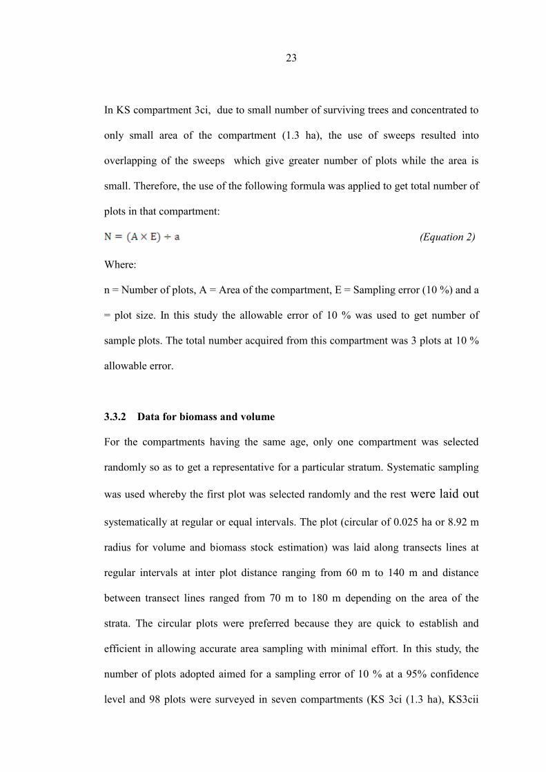
3.3.2 Data for biomass and volume ............................................................ 23
3.3.3 Destructive sampling for biomass and volume models ..................... 24
3.3.4 Laboratory work ................................................................................ 27
3.4 Data Analysis ................................................................................................... 27
3.4.1 Tree volume data preparation ............................................................ 27
3.4.2 Tree biomass data preparation ........................................................... 28
3.4.3 Model development, selection and evaluation .................................. 30
Page 10
x
3.4.4 Height diameter model development................................................. 31
3.4.5 Evaluation of previous merchantable volume to estimate tree
biomass .............................................................................................. 32
3.4.6 Computation of other forest parameters ............................................ 33
CHAPTER FOUR ................................................................................................... 35
4.0 RESULTS AND DISCUSSION .................................................................... 35
4.1 Tree Volume Models ....................................................................................... 35
4.2 Tree Biomass Models ...................................................................................... 43
4.2.1 Total tree above ground biomass model ............................................ 43
4.2.2 Total tree belowground biomass model ............................................ 47
4.2.3 Total tree biomass model................................................................... 50
4.2.4 Other biomass models ....................................................................... 53
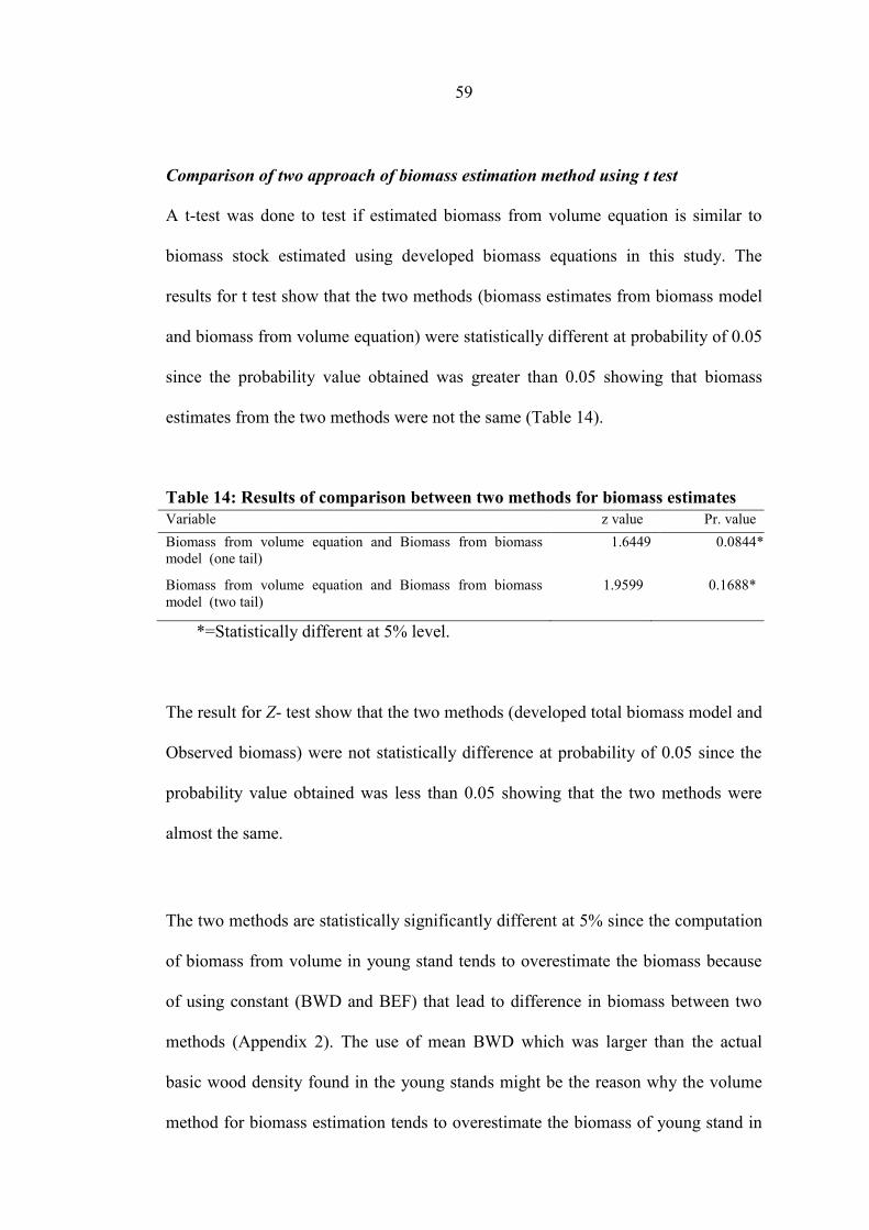
4.3 Comparison of Biomass Estimating Approaches ............................................ 55
4.4 Forest Stand Parameters .................................................................................. 60
4.4.1 Stand volume ..................................................................................... 60
4.4.2 Stand biomass .................................................................................... 65
4.4.3 Stem per ha ........................................................................................ 70
4.4.4 Basal area per ha ................................................................................ 71
CHAPTER FIVE ..................................................................................................... 73
5.0 CONCLUSIONS AND RECOMMENDATIONS ...................................... 73
5.1 Conclusions ..................................................................................................... 73
5.2 Recommendations............................................................................................ 74
Page 11
xi
5.2.1 The need to use single parameter and two parameter models for
biomass and volume estimation......................................................... 74
5.2.2 The need to conduct studies on plantation soil biomass .................... 75
REFERENCES ........................................................................................................ 76
APPENDICES ....................................................................................................... 100
Page 12
xii
LIST OF TABLES
Table 1: Statistical summary for number of sample trees (n), diameter at
breast height (Dbh) and height (ht) of sample trees ............................... 24
Table 2: Volume model parameters and performance criteria for various tree
components............................................................................................. 37
Table 3: The comparison of total tree volume with other general total tree
volume .................................................................................................... 40
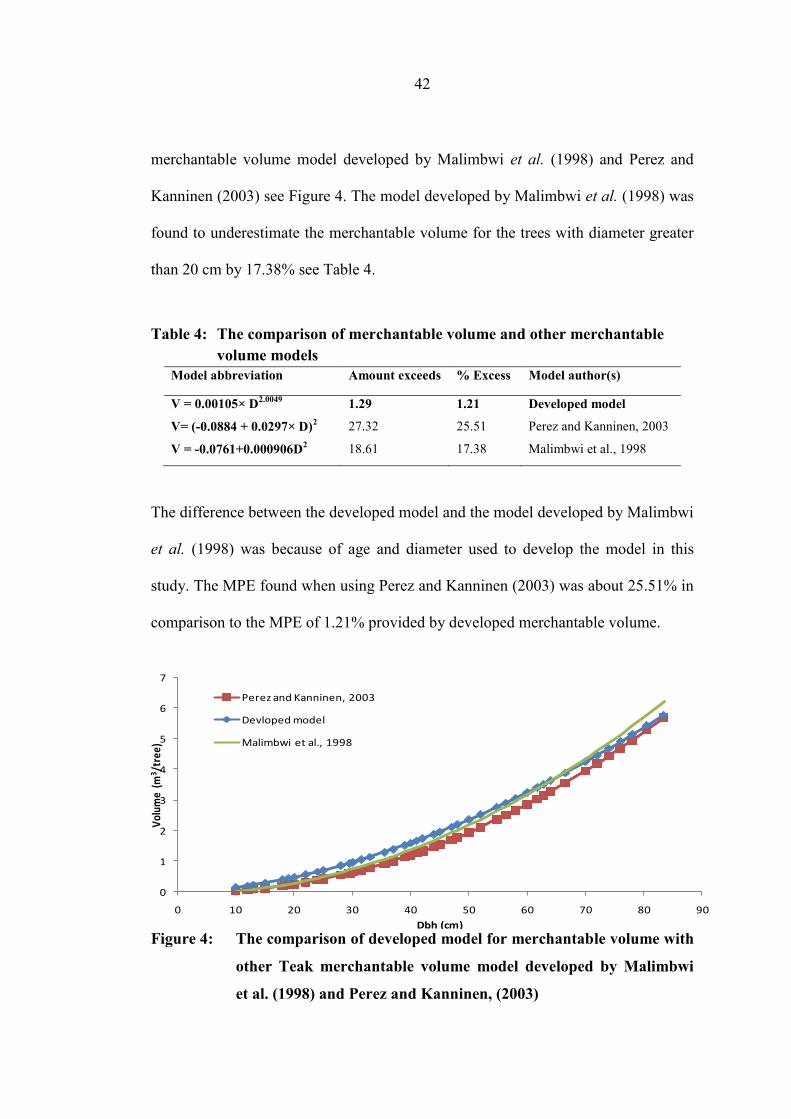
Table 4: The comparison of merchantable volume and other merchantable
volume models ....................................................................................... 42
Table 5: Biomass model parameters and their performance criteria .................... 43
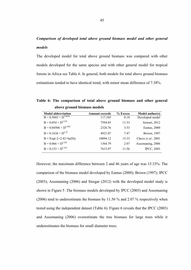
Table 6: The comparison of total above ground biomass and other general
above ground biomass models ............................................................... 45
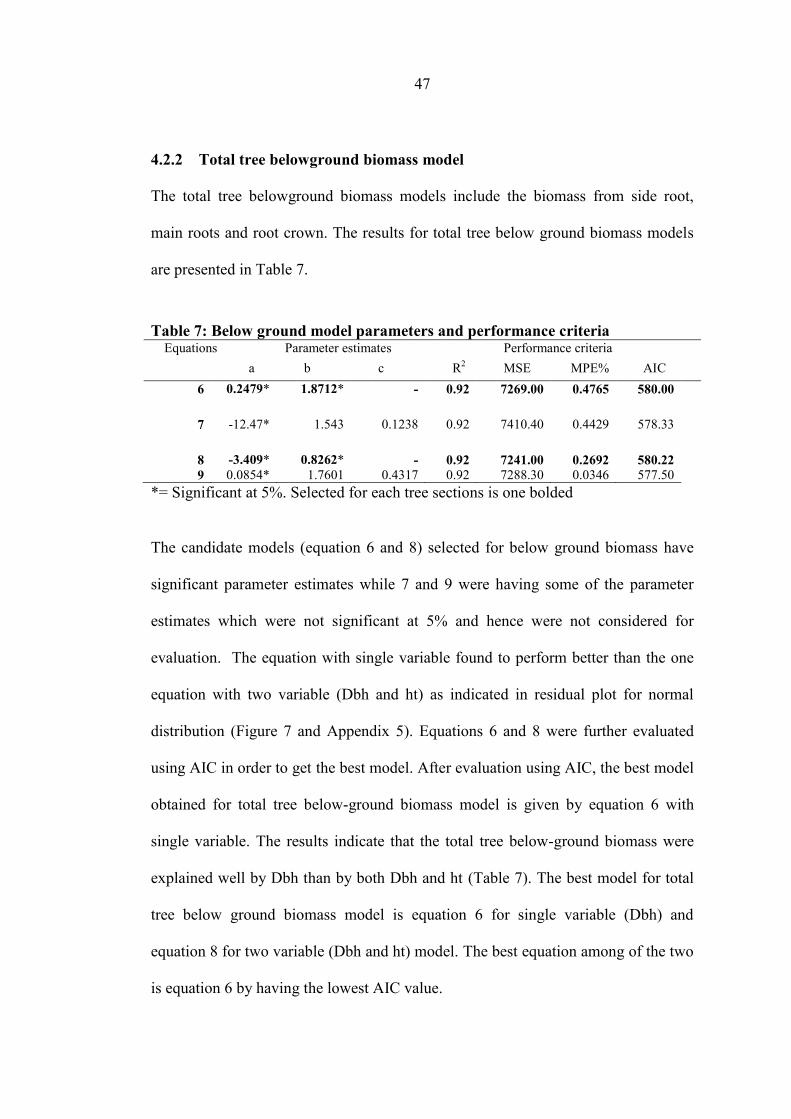
Table 7: Below ground model parameters and performance criteria ................... 47
Table 8: The comparison of total tree below ground biomass model with
other studies............................................................................................ 48
Table 9: Total below ground model parameters and performance criteria .......... 50
Table 10: The comparison of total tree biomass and other general models ........... 53
Table 11: Biomass model parameters and performance criteria for other tree
components............................................................................................. 54
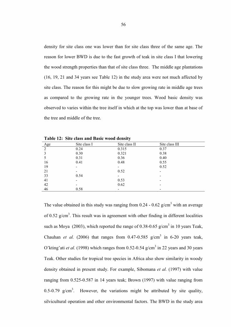
Table 12: Site class and Basic wood density .......................................................... 56
Table 13: Root to shoot ratio in the study area ....................................................... 57
Table 14: Results of comparison between two methods for biomass estimates..... 59
Page 13
xiii
Table 15: Total tree biomass, volume, stem/ha and above-ground biomass
by age ..................................................................................................... 61
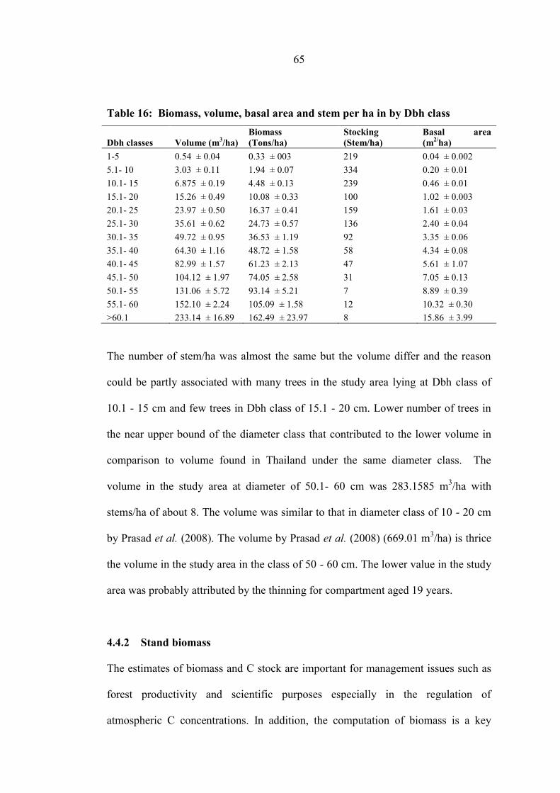
Table 16: Biomass, volume, basal area and stem per ha in by Dbh class .............. 65
Page 14
xiv
LIST OF FIGURES
Figure 1: The tree below ground components ..................................................... 27
Figure 2: Residuals plot for total tree volume, total stem volume and
merchantable volume model selected for evaluation .......................... 39
Figure 3: Comparison of developed total tree volume model with other teak
total tree volume models developed by Malimbwi et al. (1998),
Philips (1995) and Depuy and Mille (1993) ........................................ 41
Figure 4: The comparison of developed model for merchantable volume with
other Teak merchantable volume model developed by Malimbwi
et al. (1998) and Perez and Kanninen, (2003) ..................................... 42
Figure 5: The residual plot for total tree above ground biomass models
under evaluation ................................................................................... 44
Figure 6: The comparison of developed total above ground biomass model
with other Teaktotal above ground biomass models developed by
Eamus (2000); Brown (1997);IPCC (2003); Assomaning (2006)
and Siregar (2012) ............................................................................... 46
Figure 7: The residual plot for total tree below ground biomass model ............. 48
Figure 8: Comparison of developed model for belowground biomass with
other Teak total belowground biomass model given by Siregar,
(2012) and Buvaneswaran et al (2006) ................................................ 49
Figure 9: The residual plot for total tree biomass model .................................... 51
Figure 10: The comparison of developed models for total tree biomass with
other Teak total tree biomass models developed by Chave et al.
(2001); Buvaneswaran et al. (2006); Siregar (2012) ........................... 52
Figure 11: Biomass distributions in the tree parts ................................................. 69
Page 15
xv
LIST OF APPENDICES
Appendix 1: Data collection form ........................................................................ 100
Appendix 2 Tree sample data .............................................................................. 101
Appendix 3: Tree height model forms and the selected model ............................ 102
Appendix 4: Scatter plots for unselected volume model ...................................... 103
Appendix 5: Scatter plots for unselected biomass model .................................... 104
Appendix 6: Scatter plot for stem biomass model and branch biomass
models Stem biomass model ........................................................... 105
Page 16
xvi
LIST OF ABBREVIATIONS AND SYMBOLS
ABG Above-ground biomass
AIC Akaike Information Criteria
B Biomass
BEF Biomass expansion factor
BGB Below-ground biomass
BWD Basic wood density
°C Degree Centigrade
C Carbon
CDM Clean Development Mechanism
CER Certified Emission Reduction
CI Confidence Interval
CO Carbon monoxide
CO2 Carbon dioxide
Dbh Diameter at breast height
Eqn(s) Equation(s)
Exp Exponential
FAO Food and Agriculture Organisation of the United Nations
gcm-3 Grams per cubic centimetre
GHGs Green House Gases
Ht
IJ
Height
Joint Implementation
IPCC Intergovernmental Panel on Climate Change
Page 17
xvii
KH
KP
Kwamsambia
Kyoto Protocol
KS Kihuhwi Sigi
LFMP Longuza Forest Management Plan
LG Longuza Bulwa
ln Natural logarithm
m Metre
Max Maximum
m2ha
-1 Square metre per hectare
m3 ha
-1 Cubic meter per hectare
MgCha-1
Megagram Carbon per hectare
Min Minimum
MPE Mean Prediction Error
MSE Mean Standard Error
NAFORMA National Forest Resource Monitoring and Assessment
NLP Non Linear Programming
P
PES
Probability level
Payment for Environmental Services
Ppm Parts per million
R2
RSR
Coefficient of determination
Root to Shoot Ratio
REDD Reduced Emissions from Deforestation and forest Degradation
SD Standard Deviation
SE Standard Error
Page 18
xviii
SUA Sokoine University of Agriculture
t Cha-1
tons of Carbon per hectare
t ha-1
TSV
TTV
Tons per hectare
Total stem volume
Total tree volume
UNFCCC United Nations Framework Convention on Climate Change
V Volume
Page 19
1
CHAPTER ONE
1.0 INTRODUCTION
1.1 Background
According to FAO (2010), total forest area in the world occupies over 4 billion
hectares (ha) with the five countries (The Russian Federation, Brazil, Canada, the
United States of America and China) having the largest forest area accounting for
more than half of the total world forest area. Forests and woodlands cover an area of
about 675 million ha, or 23% of Africa’s land area and about 17% of global forest
area (FAO, 2011). The five countries with the largest forest area in Africa are the
Democratic Republic of Congo, Sudan, Angola, Zambia and Mozambique; together
they have 55% of the forest area on the continent (FAO, 2010). Tanzania has a total
land area of about 88.025 million ha out of which 48.4 million ha are covered by
forests and woodlands (NAFORMA, 2012). The five regions having more
significant forest areas are Morogoro, Lindi, Ruvuma, Mbeya and Tabora.
The total ´planted forests’ area worldwide is reported to be 264 million ha.
According to FAO (2010), the area of ´planted forest´ in the global South increased
more than 50% between 1990 and 2010, from 95 million to 153 million ha.
According to Ngaga, (2011) the total plantation area in Africa in year 2010 was 8
036 000 ha comprising 3 392 000 ha industrial plantations, 3 273 000 ha non-
industrial plantations and 1 371 000 ha unspecified plantations, which is around
4.3% of the global plantation area. Furthermore, FAO (2001) found that in Africa
Eucalyptus sp. is the most widely planted genus covering 22.4% of all planted area,
followed by Pinus (20.5%), Hevea (7.1%), Acacia (4.3%) and Tectona (2.6%). The
area covered by other broadleaved and other conifers is respectively 11.2% and
Page 20
2
7.2%, while unspecified species cover 24.7%. Private sector interest in plantation
development is reported to have slowly started to emerge in East Africa (Ngaga,
2011). A good example of private Teak plantation in East Africa is one in the
Kilombero Valley in Tanzania.
Large-scale establishment of exotic forest plantations in Tanzania (by then called
Tanganyika) commenced under the British rule (1920-1961) and were mainly based
on species and provenance trials, and successful inoculation with suitable mycorhiza
(Nshubemuki et al., 2001). The total gross area of forest plantations in Tanzania is
estimated to be about 552 576 ha (NAFORMA, 2012). The ownership of forest
plantations in Tanzania can be either government or private. Plantation forests under
government ownership cover about 84,615 ha (Chamshama, 2011) and private
ownership covers 450 000 ha (NAFORMA, 2012). The most important industrial
plantation species are Pines (Pinus patula, P. elliottii and P. caribaea), Cypress sp,
Eucalyptus sp and Tectona grandis.
Among all plantations in tropics, Teak (Tectona grandis) which is the focus of this
study is highly demanded. Furthermore, Teak is the world’s most cultivated high-
grade tropical hardwood, covering approximately 6.0 million ha worldwide (Bhat
and Hwan Ok Ma, 2004). Of this net area of Teak plantations, about 94% are in
Tropical Asia, (44% in India, 31% by Indonesia alone, 19% in Thailand, Myanmar,
Bangladesh and Sri Lanka) and 4.5% in Tropical Africa. The high demand for Teak
is due to the excellent properties supporting wide range of uses, including flooring,
decking, framing, cladding, fascias and barge boards. In the decorative line it can be
Page 21
3
used for lining, panelling, turnery, carving, furniture (both indoor and outdoor) and
parquetry (Oscar et al., 2006).
Among other functions, forests play a crucial role in climate change mitigation
through Carbon (C) sequestration. Thus, quantification of amounts of C stored in
various vegetation types has recently gained importance all over the world (Brown,
1997; Chave et al., 2004). The amount of C stored in the forest stand depends on its
age, volume per ha and number of stems per ha (Alexandrov, 2007; Gurney, 2008).
But due to variation of C storage by species and forests type, direct field
measurement for estimation of biomass and total C storage for specific forest
ecosystems is essential (Munishi, 2001).
1.2 Problem Statement and Justification
Carbon dioxide (CO2) is one of the more abundant greenhouse gases (GHGs) and a
primary agent of global warming (Foster et al., 2007). It constitutes 72% of the total
anthropogenic GHGs, causing between 9-26% of the greenhouse effect (Kiehl and
Trenberth, 1997). IPCC (2007) reported that the amount of CO2 in the atmosphere
has increased from 280 ppm in 1750 (the pre-industrial era) to 379 ppm in 2005, and
is increasing by 1.5 ppm per year. International efforts have addressed the issue of
climate change across all sectors and corporations to reduce GHGs emissions (Pyo
et al., 2012). To achieve this, there is a need of accurately identifying emission
levels of GHG across different sectors (Gibbs et al., 2007).
Page 22
4
Forests are known to store large quantities of C, which was one of the reasons to
include them in the Kyoto Protocol (UNFCCC, 1997; Nabuurs, 2008). Therefore,
they have the greatest potential for mitigating atmospheric CO2 emissions (Brown,
1997; Munishi et al., 2000; Munishi, 2001; Munishi and Shear, 2004). The amount
of C stored in the forest stand depends on its age and productivity (Gurney, 2008),
and species composition (Munishi, 2001; Munishi and Shear, 2004). According to
Kumar (2002), a young forest, when growing rapidly, can sequester relatively large
volumes of additional CO2 roughly proportional to the forest growth in biomass or C
stock. But due to variation of C sequestration capacity by age, species and forests
type, field measurement for estimation of biomass and total C storage for specific
forests ecosystem are essential (Munishi, 2001).
Allometric model for estimation of volume and biomass varies between sites and
species as a function of growth conditions and tree species composition. Efforts to
develop allometric equations have been increasingly in recent years in the Tropics
from global to local allometric equations (Brown, 1997; Chave et al., 2005). The use
of global allometric equations can lead to significant errors in vegetation biomass
estimations compared to local equations (Brown et al., 1989; Chave et al., 2005;
Heiskanen, 2006). Furthermore, developers of these equations often caution against
extrapolation beyond their study areas (Navar, 2002; Chave et al., 2005). In
addition, the available allometric equations for quantification of root systems are
limited to a few tree species and are not be available for many trees (Chavan, 2010).
In Tanzania, one model has been developed to quantify the amount of C and
biomass for Teak in Mtibwa Plantation forest (O’kting’ati et al., 1998). Despite of
Page 23
5
the presence of allometric models for estimation of biomass in Teak in the country,
yet the model cannot be used in wide range of diameter classes, ages, site classes,
elevation and soil type because of the following reasons. First, the allometric model
was developed from small samples (i.e. 12 sample trees). Secondly, the sample
covered a narrow diameter range (17 – 42.5 cm) that excluded small or bigger trees,
which means that in practice the model often must be applied beyond their valid
diameter ranges. Thirdly, the model was based on plantation of 22 and 30 years of
age which is about half rotation age by then. Although there are well documented
biomass models for teak elsewhere e.g. general biomass model for tropical forests in
which the Teak is inclusive in Africa (Brown, 1997; IPCC, 2003; FAO, 1997;
Chave et al., 2005), India (Buvaneswaran et al.,2006; Siregar, 2012), Ghana
(Assomaning, 2006), Australia (Eamus, 2000), their applications in Tanzania are
limited due to differences associated with altitude, soil type (Brown and Lugo, 1992;
Tuomisto et al., 1995; Slik et al., 2010; Baraloto et al., 2011; Laurance et al., 1999),
topographic position (Austin et al., 1996; Macauley et al., 2009), disturbance regime
(Lugo and Scatena, 1996), age of tree (Kumar, 2002; Alexandrov, 2007),
provenance (Macauley et al., 2009), and climatic conditions (Gentry, 1982; Girardin
et al., 2010).
This suggests the need for development of local reliable biomass models for both
above and belowground for Teak that can account for the biomass variation as a
function of diameters, age classes, site classes and height. The developed biomass
models will enhance decisions by forest managers when developing management
plan. In addition, the developed biomass models are important for the emerging C
credit market mechanism such as Reducing Emission from Deforestation and Forest
Page 24
6
Degradation (REDD+), and the role of conservation, sustainable management of
forests and enhancement of forest carbon stocks and Clean Development
Mechanism (CDM). The core idea of REDD+ is the role of conservation, sustainable
management of forests and enhancement of forest C stocks at multilevel (global-
national-local) system through payments for environmental services (PES).
Furthermore, volume models which are able to quantify merchantable tree volume
and total volume are also required when trees are warranted for commercial
purposes. Similar shortcomings stated for previous developed biomass models also
apply to volume models. Since the previous volume models (Malimbwi et al. (1998)
and Van Zyl (2005)) may either underestimate or overestimate volume thus subject
to uncertainty of benefits to a seller or a buyer.
This study was carried out at Longuza teak plantation which has a wide range of tree
ages, site classes, diameter classes and altitudes. Studies across broad ranges of
growth conditions are particularly valuable because they provide broad range of
biomass and volume variations which may result into reliable biomass or volume
models.
1.3 Research Objectives
1.3.1 Main objective
To develop volume and biomass estimation models for Teak at Longuza forest
plantation in Tanzania
Page 25
7
1.3.2 Specific objectives
i) To develop models for estimating volume of Teak.
ii) To develop models for estimation of above and below ground biomass of
Teak.
iii) To compare biomass estimates computed from developed biomass model and
the estimates derived from developed volume equation by Malimbwi et al.
(1998).
iv) To determine forest structure attributes (stand volume, biomass, basal area
and trees per ha)
Page 26
8
CHAPTER TWO
2.0 LITERATURE REVIEW
2.1 History or Introduction of Teak in Tanzania
Teak is a large sized deciduous tree indigenous to the greater part of Burma, the
Indian peninsula and west parts of the Thailand and Cambodia (O’kting’ati et al.,
1998). It is a tree species growing in moist and dry tropical regions at elevation
between sea level and 1300 m above sea level. The first recorded planting of Teak in
Tanzania was done by Germans in 1898 using seeds from Calcutta which were
planted at Dar es Salaam and Mhono in the Coast region (Wood, 1967). Thereafter
seeds from Java, India and Thailand were distributed to many lowland stations in the
country and were planted in field trial plots (Wood, 1967). Large scale planting of
Teak in Tanzania started in 1960/61 at two sites, Longuza forest project in Tanga
region and Mtibwa forest project in Morogoro region. The Longuza forest plantation
was established by the colonial British government in 1952 as a gap planting activity
to replace the exploited species in the natural forest. In 1961, the Forest Department
was forced to drop the idea of gap planting and replaced it with the growing of fast
growing hardwood species like Teak in order to meet the supply of wood material to
satisfy the rapidly increasing local and export wood demands.
2. 2 The Role / Function of Forests
The forests (natural and plantations) are habitat for different biodiversity with a wide
range of both socio-economic and ecological values. The forests are keys in
sustaining the biodiversity of natural ecosystems and in regulating the world’s
climate system (Chidumayo et al., 2011). Moreover, forests comprise an important
Page 27
9
C reservoir, since they store about twice the amount of C present in the atmosphere
(Canadell and Raupach, 2008). Recently, adverse impacts of change in climate on
the environment, human health, food security, human settlements, economic
activities, natural resources and physical infrastructure are already noticeable in
many countries, including Tanzania (Chidumayo et al., 2011). Forests contribute to
climate change mitigation by removing atmospheric CO2 and storing it in different C
pools (i.e., biomass, soil, dead organic matter, litter) (IPCC, 2006).
The ultimate objective of The United Nations Framework Convention on Climate
Change (UNFCCC), in which Tanzania is a member, is to stabilize the atmospheric
GHG concentrations at the level that will not cause dangerous anthropogenic
interference with the climate system. There are two alternatives to reduce CO2:
decreasing C source and increasing C sink. Forests are known to be a major C sink
that store large quantities of C (650 billion tons of C, 44% in the biomass, 11% in
dead wood and litter, and 45% in the soil (FAO, 2010)), which was the one of the
reasons for forests to be included in the Kyoto Protocol (UNFCCC, 1997; Nabuurs,
2008). Therefore, forests have the greatest potential for mitigating atmospheric CO2
emissions (Munishi et al, 2000; Munishi, 2001; Munishi and Shear, 2004).
Forests are major renewable natural resource on the earth and provide a wide range
of economic, social, environmental, and cultural benefits. The world forest survey of
2010 has noted that the planted Teak forests are predominantly young due to
increase plantations from 95 million to 153 million since 1990 (FAO, 2010). The
prevailing age class distribution in the world is an indication of increased efforts to
Page 28
10
establish and manage planted Teak forests in the past 20 years and this pattern is
very likely to persist in the future (FAO, 2010). Forest plantation establishment and
ecosystems management practices can play a significant role in climate change
mitigation if they are managed for such purposes.
2.3 Tree Volume
Volume estimation is necessary for understanding different utilization standards. For
plantation forests, many growth and volume studies have been previously done with
a focus on merchantable volume (Malimbwi, 1987; Malimbwi and Mbwambo, 1990;
Malimbwi et al., 1998). Tree volume provides valuable information on supply of
both industrial wood and hence identifying sustainable management of forests and
woodland ecosystems (Chamber et al., 2001, Mugasha et al., 2012). Furthermore
tree volume provides information about health and value of a given stand. The
volume values reported by various studies at different Teak ages includes the study
at 2 years old Teak by KFRI (2011) with volume value ranging from 1.87 - 6.57
m3/ha, at age of 5 years by Perez and Kanninen (2005) in Costa Rica the values was
28.4 - 32 m3/ha, by Perez (2005) at age of 16 volume of 420.33 – 466.35 m
3/ha and
at 40 years by KFRI (2011) of about 236 m3/ha. A study by Zambrana (1998)
estimated the volume at age of 4, 10, 17 and 25 years by using volume equation to
be 22 m3/ha, 89 m
3/ha, 159 m
3/ha and 214 m
3/ha respectively. Furthermore, on study
by Picado (1998) in Costa Rica estimated the volume of 48.59 m3/ha, 140.04 m
3/ha
and 198.87 m3/ha at age of 8, 15 and 20 years respectively. Therefore, appropriate
methods and approaches to quantify the stand volume is mandatory at different age
classes and site since volume varies with location, silvicultural operation, site classes
and age.
Page 29
11
2.4 Tree Biomass
Forests in particular play a key role in C cycle and in maintaining climatic balance.
Forests and woodlands are important C sinks and sources containing majority of the
above ground terrestrial organic C. International negotiations to limit greenhouse
gases require understanding of the current and potential future role of forest C
emissions and sequestration in both managed and unmanaged forests (Pan et al.,
2011). Tanzania has reported an average C stock value of 60 t C/ha in living forest
biomass (FAO, 2010). The forests in Tanzania can also be used for climate change
mitigation if are well managed. The Kyoto Protocol (KP) of UNFCCC was
developed as an attempt to confront and begin to reverse the rising CO2
concentrations (Pearson and Brown, 2005). The KP was adopted in 1997 and
entered into force in 2005 with establishment of innovative mechanisms to assist
developed countries to meet their emissions commitments (UNFCCC, 2007). The
Protocol created a framework for the implementation of national climate policies,
and stimulated the creation of the C market and new institutional mechanisms that
could provide the foundation for future mitigation efforts (Geoff, 2009). The
Protocol has flexible mechanisms through which developed countries can achieve
their emissions reduction commitments (Chidumayo et al., 2011). These include
Emissions Trading, Joint Implementation (JI) and the CDM. Of interest to African
forestry is the CDM which allows developed countries to invest in green projects
that reduce C emissions in Africa and other developing countries (UNFCCC, 2007).
The CDM is an arrangement under Article 12 of the KP of the UNFCCC (UNFCCC,
2007). The purpose of the CDM was to assist developed countries in achieving
sustainable development and in contributing to the ultimate objective of the
Page 30
12
convention, and to assist developed countries in achieving compliance with their
quantified limitation and reduction commitments (UNFCCC, 2007). This allows
developed countries with a GHGs reduction commitment and developing countries
to jointly undertake emission reduction project activities in developing countries that
contribute to sustainable development and result in certified emission reduction
(CER) (UNFCCC, 2007). The C market aims to decrease emissions of GHGs which
scientific evidence shows in all likelihood to be contributing to global warming and
climate change. The selling of C credit obtained from afforestation and reforestation
project was seem to be one of the incentives to motivate local community to be
involve in climate change mitigation. C credits earned via conservation are best
suited for trade in the voluntary C market where buyers place high value on the
sustainability of a project, often paying a premium for C removal which provides
benefits for rural livelihoods. C credits are the unit of trade used in the C market,
where one C credit represents one ton of CO2 that has been removed from the
atmosphere or has been prevented from entering the atmosphere (IPCC, 2003).
However, the key requirement of C trading mechanism is the availability of
individual tree biomass equations to facilitate the computation of baseline and the
change of C. The Voluntary Carbon Standard (VCS) follows the format of CDM but
does not require authorization by the host country which greatly reduces transaction
costs. Currently there are few projects (example Kilombero Teak Company)
registered under CDM in Tanzania with challenge of quantifying C using a general
equation developed from other nations.
Page 31
13
2.5 Methods of Estimating Tree Volume and Biomass
2.5.1 Tree volume estimation
There are two methods for tree volume estimation in forest plantations namely
destructive methods and non-destructive methods. Destructive method is very
common approach for estimating volume of standing trees. This method involves
felling of sample trees measuring the length and mid diameter of the different
components of the harvested trees like tree stem and branches (Malimbwi et al.,
1998). Due to differences in allometry and tree architecture, species specific volume
models are often preferred (e.g. Ketterings et al., 2001). The total tree and
merchantable volume in the study area had been developed by Malimbwi et al.
(1998). However, accurate computation of volume at the final harvest depends
largely on the availability of individual tree volume equations. With increasing
demand and availability of Teak, it is essential to develop appropriate volume
allometric models in order to quantify the amount of poles, lumber, firewood and
other wood products in terms of volumes for efficient pricing and utilization of
wood from juvenile wood to mature wood. Volume estimation models provide
valuable information on supply of both industrial wood and hence identifying
sustainable management of forests and woodland ecosystems (Chamber et al., 2001,
Mugasha et al., 2013a). Malimbwi et al. (1998) developed equation for estimation of
Teak volume with a narrow range of tree diameter (5 – 65 cm).
Non-destructive method involves the multiplication of the tree basal area by the tree
height and form factor (e.g. Munishi and Shear, 2004). Form factor is one method for
harmony a relation between tree form and volume and is defined as the ratio of tree
Page 32
14
real volume to volume of one geometrical form such as cylinder, cone and or
truncated cone that its diameter and height are near to tree (diameter of geometrical
from is equal to diameter at breast height and its height is equal to tree height).
Volume obtained from this way has the advantage of getting quick results but suffer the
problem of accumulated error resulting from the prediction of height. The study on
form factor was done by Malimbwi et al. (1998) at Mtibwa and Longuza forest
plantation during development of volume equation. Also, a number of studies have
reported standing volume of teak by using non destructive and destructive methods.
For example teak standing volume estimated by volume equations have been
reported by Hamzah and Mohamed (1994) for Mata Ayer in Malaysia; by
Chakrbarti and Gaharwar (1995) for Karnataka, Madhya Pradesh, by Moret et al.
(1998) for Venezuela; by Nunifu and Murchinson (1999) for northern Ghana and by
Phillips (1995) in Sri Lanka.
2.5.2 Tree biomass estimation
There is no single method for estimating biomass stocks, but there are number of
methods depending on the scale accuracy considered (Gibbs et al., 2007). There are
two main common methods for estimation of biomass namely ground based and
remote-sensing. Ground based biomass can be either aboveground or both above and
below ground biomass estimation. The above and below ground biomass estimation
can either be destructive or non-destructive methods. The non-destructive method
estimates biomass as a product of volume and wood basic density where tree volume
is a function of basal area and tree total height. Non-destructive method also may
involve remote sensing technology. The remote sensing methods provide broad
Page 33
15
geographic coverage; they are reliant on good quality of ground-truthing data for
calibration and verification (Mitchard et al., 2011).
The destructive sampling involves falling and excavating of tree, crosscutting into
manageable size, weighing the billets as well as roots, taking samples for oven dry
to fresh weight determination and finally establishing the relationship between dry
weight of tree and easily measurable tree parameters such as basal area, diameter at
breast height (Dbh), height or both. The destructive method is believed to produce
high accuracy in estimating the tree biomass (Brown, 1997; Seifert and Seifert,
2013). Also, it has been established that site and species specific biomass estimates,
obtained from locally developed equations provide estimates of C with greater
certainty (IPCC, 2006); that is why biomass equations for specific species and site
specific need to be developed.
2.5.2.1 Biomass estimation from allometric equation
The most common procedure used for estimating individual tree biomass is to relate
biomass and easily measurable tree parameters by means of regression equation
(Brown, 1997). Biomass non-linear or linear equations are usually fit using least
squares estimates of regression parameters where the candidate models are selected
first. Before a model is accepted for further analysis, its variance ratio must be
significant at the chosen level of probability and plot of residuals must have constant
variance and no bias. Similarly a plot of measured against estimated biomass should
show no bias. However, according to Canadell et al. (1996), Levang-Brilz and
Biondini (2002) and Jackson et al. (1996) there are no current models for predicting
Page 34
16
belowground biomass based on measurements of aboveground biomass across
diverse species. Allometric models for estimation of biomass and C stored in
different forests and woodlands are still uncertain in developing countries due to
lack of specific allometric models for biomass estimation (Chave et al., 2005;
Houghton, 2005). Also, it has been established that site and species specific biomass
and C stock estimates, obtained from locally developed equations provide estimates
of greater certainty (IPCC, 2006). There has been an effort to establish the Teak
allometric model in Tanzania. A study conducted by O’kting’ati et al., (1998) on the
potential of Tectona grandis at Mtibwa to act as a C sink found that Tectona grandis
stored between 595 ton CO2/ha and 844 ton CO2/ha. The strength of the study
conducted by O’kting’ati et al., (1998), is that biomass estimates were based on site
and species specific equations; both belowground (roots) and aboveground tree
components (stem, branches, twigs and leaves) were included in the study. Biomass
and C stocks estimation equations developed for Tectona grandis in Mtibwa forest
plantations by O’kting’ati et al. (1998) have a number of shortcomings. First, they
were developed from a small sample (i.e. 12 sample trees), cover narrow range of
diameters (17 - 42.5 cm), data covering limited variation regarding growth
condition, silvicultural treatments and exclude large trees as well small trees (young
trees). According to Brown and Lugo (1992) the regression equations must include
wide range of tree size to represent all variation of biomass from the smallest tree
diameter to the largest tree diameter. From these facts, site specific and species
specific is needed covering wide range of tree size to quantify the biomass of Teak
in Tanzania. These equations are of great importance for the estimation of tree
biomass and then to estimate forest C stock and C stock changes. The quality of
Page 35
17
these equations is crucial for ensuring the accuracy of forest biomass and C
estimates in the plantation.
2.5.2.2 Biomass estimation from tree volume
The total biomass estimated from tree volume uses basic wood density (BWD),
biomass expansion factor (BEF) and root to shoot ratios (RSR). These parameters
are essential in estimating the total tree biomass without destroying trees. The BWD
defined as the ratio of oven dry mass and its fresh stem wood volume without bark
(IPCC, 2006). The BWD is an essential component for estimating forest C stocks as
it varies among tree genus and species (Chave et al., 2006). The BWD of Teak was
determined by O’kting’ati et al. (1998) in Mtibwa forest plantation and Sibomana et
al. (1997) in Longuza forest plantation. The study by O’kting’ati et al. (1998) was
based on Teak aged 22 and 30 years with BWD of 0.52 - 0.54 gcm-3
. The study by
Sibomana et al. (1997) in Longuza forest plantation at age of 14 years recorded
BWD of 0.525 – 0.587 gcm-3
. Another study by Izekor et al. (2010) in Malaysia at
age of 15, 20 and 25 years found the value of BWD of 0.48 gcm-3
, 0.56 gcm-3
and
0.65 gcm-3
respectively indicating the BWD varying with age, site class, location,
soil type, silvicultural operation and slope. Consequently, IPCC recommended
development of BWDs that reflected the influence of regions and ages (IPCC,
2006).
The BEF is computed by dividing total biomass of aboveground tree components
(stem, branches and twigs) to biomass of stem (Brown, 1997). Essentially, BEF is
used to estimate biomass of other parts which are not covered during biomass
measurement. The BEFs from inventories in tropical Asia, America, and Africa
Page 36
18
were reported to be 1.1 and 2.5 (Brown and Lugo 1992;, 1997). The BEF differs
between sites (Wirth et al., 2004) and ages (Lehtonen et al., 2004). The mean value
for the BEF of Teak was ranging from 1.4 - 1.8 (Sengura and Kanninen, 2004). The
value for BEF given by Guendehou et al. (2012) at Teak of 3 - 15 years was
between 1.28 and 1.46. From these studies it is very clear that BEF varies with age
and site and hence it is better to find the BEF across various ages found in the study
area.
The RSR is obtained by dividing biomass of total belowground tree components to
biomass of total aboveground tree components. The value of RSR of Teak reported
by Brown (1997) is 0.20 and Perez and Kanninen (2003) ranges from 0.11 - 0.23 for
20 years old teak. This finding showed the variation of RSR with tree age with the
highest value for young age and the lowest value for old Teak. Although other
authors, such as Cairns et al. (1997) and Mokany et al. (2006) did not find any
differences between groups of species in RSR (softwood and hardwood) and they
give a value of 0.26. Pearson and Brown (2005) observed that the RSR varies with
age in which the young tree had shown to have large value of RSR in comparison to
the old tree. Further study by Hase and Forster (1983) observed that the RSR
decreased in value with increase in tree age from 0.42 at age of 4 years to 0.20 at age
9 years. In Tanzania no studies had been done for computation of RSR across
various ages of Teak.
2.6 Other Stand Parameters
The estimation of other forest parameters are often carried out to describe
characteristics of forest plantation during study time. Basal area is a useful measure
Page 37
19
of stocking. Basal area is defined as the sum of cross-sectional area measured at
breast height of all trees in a stand, expressed as m2ha
-1. Furthermore, basal area
provides other information needed for tending operations such as whether or not
thinning should be conducted. A study conducted by Sunanda and Jayarame (2006)
at age of 2 and 42 years observed the basal area was ranging from 0.3 m2ha
-1 to
51.98 m2ha
-1 on young Teak of one year to old Teak stand. Further, study by
Robertson and Reilly (2005) on performance of 14 and 16 year old Teak found the
basal area ranging from 8.4 to 14.2 m2ha
-1 at age of 14 years and from 9.1 to 14.5
m2ha
-1 at age of 16 years. The number of stems per hectare, (N) is a useful parameter
for defining stocking if it is accompanied with information on age, mean height or
diameter. The manipulation of the number of stems per ha through thinning can be
used to control the growth of individual trees for provision of tree sizes for specific
utilization standards (Malimbwi, 1997).
Page 38
20
CHAPTER THREE
3.0 MATERIALS AND METHODS
3.1 Location of the Study Area
Longuza Forest Plantation has total area of 2 449 ha. Out of this area 1809.8 ha is
plantation forest and 639.2 ha is under natural forest. It is situated 17 km from
Muheza town and 52 km from Tanga port on the Eastern foothills of the East
Usambara Mountains, which is Amani Nature Reserve and part of the Eastern Arc
Mountains between latitudes 4º55’ and 5º10’ South and Longitudes 38º 40’ and 390
00’ East. The mean annual rainfall for Longuza plantation is about 1500 mm with a
mean annual temperature of about 270C (Van Zyl, 2005; Ngaga, 2011).
Longuza Forest plantation lies at altitudes between 160 and 560 meters above sea
level (Sibomana et al. 1997; Van Zyl, 2005; Ngaga, 2011). The plantation is covered
geologically by the Usambara rocks which are Pre – cambian and assigned to old
Usagara basement complex system. The crystalline rocks underwent several cycles
of folding, metamorphism and finally migmatization (Van Zyl, 2005; Ngaga, 2011).
The soil is dominated by loam soil which is easily accessible to cultivation
(Malimbwi et al, 1998; Ngaga, 2011). The dominant species in natural vegetation
include Khaya anthotheca, Newtonia paucijuga, Albizia gummifera, Combretum
schumanni, Brachystegia sp., Isoberlinia sp., Pterocarpus angolensis, Milicia
excelsa, Antiaris sp., Zanha sp., Sterculia sp. and Acacia sp. (Sibomana et al. 1997;
Van Zyl, 2005).
Page 39
21
3.2 Structure of the Plantation
3.2.1 Management units
The forest plantation is managed in units of different sizes, ages and species, which
are known as compartments. There are three ranges/blocks namely
Kihuhwi/Kwamsambia (KH); Kihuhwi - Sigi (KS) and Longuza/Bulwa (LG). Each
range/block is subdivided into compartments and these compartments are numbered
1, 2, 3 etc. The planted area for Teak is about 1709.8 ha and the rest of planted area
is planted with Teminalia sp., Cedrella sp., Mellia azadirach and Milicia excela
(LFMP, 2013). The plantation is divided into three site classes namely KS being site
class I of about 553.2 ha, KH in site class II of about 592.6 ha and LG in site class
III having 564 ha. Each range/block was subdivided into compartments having trees
with different ages. There are research plots established by TAFORI and SUA
located within the forest plantation. These include Kihuhwi seed stand of about 31.6
ha planted in 1906, International teak provenance at Kihuhwi/Sigi planted in 1960,
hardwood arboretum situated in Bulwa having 68 different trees species and spacing
trial planted in 1996 and 1998 respectively.
3.2.2 Age distribution and status of the plantation
The Teak plantation is dominated by Old aged Teak (Over half of the area). The age
distribution of the plantation is not normal, which means the forest age is not
normally distributed. The plantation has more area (more than half of the area
planted Teak) for old trees greater than 20 years than young trees. Most of the
compartments have trees with good form except, those compartments which were
not tended in the past due to lack of funds. The health of forest stand is good except
there are few deaths of trees in some compartments due to maturity.
Page 40
22
3.3 Data Collection
3.3.1 Reconnaissance survey
Reconnaissance survey was carried out for deciding number of plots per each
compartments and to eliminate those compartments which were impractical or
unfeasible.
According to Chave et al. (2004), the number of sampling plots should be
determined based on area and homogeneity of vegetation. So in this study; stratified
sampling design was used in which the plantation was classified into six strata
according to age and site classes. These strata were 1-5 years, 6-10 years, 11-15
years, 16 -20 years, 21-25 years and greater than or equal to 26 years. All strata were
having all site classes (KS site class I, KH site class II and LG class III) found in the
plantation.
Random sampling was employed in the selection of strata because there were
several compartments having the same characteristics of interest in the study area.
The total number of plots in each stratum was determined by estimating basal area
using relascope in which a minimum of 15 sweeps were done in each stratum and
the number of plots was obtained using equation 1.
n = cv2t2/E
2 (Equation 1)
Where:
n = number of plots; cv2 = coefficient of variation (standard deviation/sample mean);
t = value of t obtained from n-1 degrees of freedom of the preliminary study at 5 %
probability in the t table and E = sampling error of 10 %.
Page 41
23
In KS compartment 3ci, due to small number of surviving trees and concentrated to
only small area of the compartment (1.3 ha), the use of sweeps resulted into
overlapping of the sweeps which give greater number of plots while the area is
small. Therefore, the use of the following formula was applied to get total number of
plots in that compartment:
(Equation 2)
Where:
n = Number of plots, A = Area of the compartment, E = Sampling error (10 %) and a
= plot size. In this study the allowable error of 10 % was used to get number of
sample plots. The total number acquired from this compartment was 3 plots at 10 %
allowable error.
3.3.2 Data for biomass and volume
For the compartments having the same age, only one compartment was selected
randomly so as to get a representative for a particular stratum. Systematic sampling
was used whereby the first plot was selected randomly and the rest were laid out
systematically at regular or equal intervals. The plot (circular of 0.025 ha or 8.92 m
radius for volume and biomass stock estimation) was laid along transects lines at
regular intervals at inter plot distance ranging from 60 m to 140 m and distance
between transect lines ranged from 70 m to 180 m depending on the area of the
strata. The circular plots were preferred because they are quick to establish and
efficient in allowing accurate area sampling with minimal effort. In this study, the
number of plots adopted aimed for a sampling error of 10 % at a 95% confidence
level and 98 plots were surveyed in seven compartments (KS 3ci (1.3 ha), KS3cii
Page 42
24
(3.1 ha), KS 5 (53.7 ha), KH1A (60.9 ha), KH9 (10.9 ha), LG58B (4.4 ha) and
LG11A (10 ha)) covering the youngest stand (2 years) up to the oldest stand (46
years) found in the forest plantation. In each plot, all trees were measured for Dbh
and only three trees (large, medium and small diameter) were measured for total
height. Other recorded data describing the plot were: altitude, slope, soil type, plot
coordinates and age (see Appendix 1 data collection form).
3.3.3 Destructive sampling for biomass and volume models
A total of 51 trees were selected purposively for model development and validation
(Table 1). The selected trees cover the diameter distribution in Longuza forest
plantation from 1 cm to 83.4 cm. The selection of trees for destructive sampling was
based on measured diameter for all the trees in the 98 sample plots. The inventory
data were distributed into eight diameter classes starting from 1-10 cm, 10.1-20 cm,
20.1-30 cm, 30.1-40 cm, 40.1-50 cm, 50.1- 60 cm, 60.1-70 cm and greater than 70.1
cm. The number of trees sampled was determined based on the ratio of trees within
each diameter class, while for the larger diameter of > 50 cm, at least five to six
trees were sampled.
Table 1: Statistical summary for number of sample trees (n), diameter at
breast height (Dbh) and height (ht) of sample trees
n Dbh (cm) Ht (m)
Mean Min. Max. SD Mean Min. Max. SD
51
37.40
1
83.4
24.53
25.65
1.5
37.50
11.00
In each diameter class, trees were selected to cover all three site classes found in the
plantation e.g. diameter class ranging from 1 - 10 cm had a total of 8 trees with
Page 43
25
distribution of three trees from site class I, three trees from site class II and two trees
from site class III. The trees for destructive sampling were measured for Dbh, total
height and root collar diameter (15 cm height from the ground) before felling and
then felled. Total tree bole height was measured again on the felled tree to ensure
accuracy. The standing height before felling was used as independent variable in
model development. Stems (including branches) were trimmed and cross cut into
manageable billets ranging from 27 cm to 270 cm depending on taper and weight.
The branches were classified into three classes (Large branch with mid diameter >
10 cm, medium branch size with mid diameter < 10 cm to > 5 cm and small branch
with mid diameter ≤ 5 cm to 2 cm). In order to minimize the effect of taper, the
billets with almost equal bottom and top diameters were measured for mid diameter.
Three small samples i.e. one at Dbh, one in the middle of the tree and last one near
the top of the stem from bark to pith were extracted. Three samples i.e. one from
large branch, one from medium branch and one from small branch were extracted.
Twigs and leaves were collected and tied into bundles and were weighed for fresh
weight. Two small samples (of about 2 cm thickness) and one sample with three to
four leaves were taken.
For below ground components (see Figure 1) once excavated, the main belowground
components were treated as follows:
(a) Stump/root crown was cleaned from soil, weighed for fresh weight and two
samples were taken for dry weight determination in the laboratory.
(b) All broken roots (roots not excavated) were measured for base diameter at
breakage point on the root crown.
Page 44
26
(c) From each sample tree, 3 main roots (small, medium and large) were selected
and traced to minimum diameter of 1 cm. The sampled roots were detached
from root crown and base diameters were measured and weighed. All sampled
roots were weighed for fresh weight. When main roots enter obstacles (stone
or another tree), the end point diameter was measured. One sample from large
root, one sample from medium root and one sample from small root were
taken for oven dry weight determination in the laboratory. For main root with
side roots, three side roots were selected and traced to minimum diameter of 1
cm and weighed for fresh weight while other side roots were measured for
base diameters. Three samples from side roots covering small, medium and
large roots if present were taken for oven dry weight determination in the
laboratory.
All billets from stems, branches, sample roots and tied bundle of twigs and leaves
were measured for weight. Also samples from stem, branches, twigs and leaves as
well as from belowground were labelled and measured for fresh weight using
electronic balance. Finally all samples were taken for further analysis in the
laboratory.
Page 45
27
Upper soil layer
Stump height
Root crown
Main root Side roots
Figure 1: The tree below ground components
3.3.4 Laboratory work
The collected samples except parts with some leaves were soaked for about eight to
ten days until they attained constant weight. Then fresh volume of each sample was
determined by water displacement method. Water displacement method minimizes
the error in estimating the volume of the disk. The samples for stem and branches
were put in oven and dried to constant weight at 103 °C for 72 to 96 hours and then
measured for dry weight. The root samples were oven dried to constant weight at 78
°C to 80 °C for 72 hours. The twigs and leaves were dried at 60 to 65 °C for about
48 hours and measured for dry weight.
3.4 Data Analysis
3.4.1 Tree volume data preparation
The individual billet volume of respective tree section (stem and branches) were
calculated using Huber’s formula (Loetsch et al., 1973). The sum of all billets of
Page 46
28
similar tree component were computed. The tree top volume was determined by
using cone formula. Because it was difficult to measure the volume of twigs (< 2 cm
in diameter), the total tree volume equation did not consider the volume of twigs.
Total individual tree volume was obtained as the sum of tree stem, branches and
cone volume as follows:
Vtot = Vstem +VL-branch+Vm-branch+VS-branch+Vcone (Equations 3)
Where:
Vtot = Total tree volume (m3), Vstem = volume of a stem (m
3), VL-branch = volume
of large branch (m3), Vm-branch = volume of medium branch (m
3), VS-branch =
volume of small branch (m3) and Vcone = volume of tree top (m
3).
Individual total tree volume (stem + branch) and stem volume (stem without
branches) was computed at three minimum diameter limit i.e. 2 cm, 5 cm, and 10
cm.
3.4.2 Tree biomass data preparation
The biomass of each tree sections (stem, branch and twigs and leaves) was
calculated as a product of its total fresh weight with its respective ratio of oven dry
weight to fresh weight. The total tree aboveground biomass was computed as the
summation of dry weight from stem, branch, and tied bundle of twigs and leaves.
For belowground section, the ratio of oven dry to fresh weight from side roots was
multiplied by fresh weight of total side root. The models were developed using their
total side root biomass through regressed with their base diameter using PROC
NLIN, a procedure in SAS software (SAS Institute Inc., 2004) to compute models
Page 47
29
parameters. There are two forms of models subjected to this stage having only
diameter as parameter for finding its parameter estimates. The best model was
selected by examining p-values (significant at p-value < 0.05), the mean square error
(MSE), the coefficient of determination (R2) and percentage mean prediction error (e
%). The side roots model developed was used to estimate unexcavated side roots
from sampled side roots. The side root model was:
B = 0.1482D1.4822
(Equation 4)
Where:
B = Side root biomass (Kg); D = Side root base diameter (cm) (e% = 2.56, MSE =
0.76 and R2 =0.71).
The total main root biomass was obtained as the summation of side root biomass
(excavated and unexcavated) and the biomass of the sampled main root. Similar
procedure was done for the best model selection as for side root. The main root
model was used to estimate the biomass of unexcavated roots from root crown. The
main root model was:
B = 0.1005×D1.6468
(Equation 5)
Where:
B = Main root biomass (Kg); D = Main root base diameter (cm) (e% = 0.30, MSE =
11.73 and R2 =0.81). All e% for both side root and main root were found to be non
significant at 5%.
Page 48
30
The total below ground biomass was given as the summation of biomass from three
sampled main roots biomass (all side roots, three sample roots), biomass from
unexcavated main root roots and biomass from root crown.
3.4.3 Model development, selection and evaluation
The four general forms of models (two model forms include Dbh only and two other
models include both Dbh and height) were fitted to tree volume and biomass. The
model forms were as follows:
B/V=a×Dbhb (Equation 6)
B/V=a+b×Dbh+c×Dbh2
(Equation 7)
B/V=Exp (a+b×ln (ht×Dbh2)) (Equation 8)
B/V=a×Dbhb×ht
c (Equation 9)
Where:
B = Biomass (Kg), V = Volume in (m3), Dbh = diameter at breast height (cm), ht =
total tree height (m) and a, b and c are model parameters.
Volume of 51 (see Appendix 2) were used for volume model development and
similar trees biomass (above ground and below ground) was used for biomass model
development. All tree volumes and tree biomass were fitted by using PROC NLIN, a
procedure in SAS software (SAS Institute Inc., 2004) to compute models parameter.
The candidate model was selected by examining p-values (significant at p-value <
0.05), the mean square of the error (MSE), the coefficient of determination (R2),
percentage mean prediction error (e %) and by plotting the residuals (observed
minus predicted values) against Dbh. For the good candidate model, the mean
prediction error should not differ from zero so that the prediction is unbiased.
Page 49
31
The study aim to select two candidate models i.e. one candidate model with Dbh
only and the other candidate model with Dbh and ht.
The candidate models were further evaluated by using Akaike Information Criteria
(AIC) which takes account of number of parameters the model has and the equation
is given as follows:
AIC=-2logL+2p (Equation 10)
Where:
p = parameters and L= Log of likelihood
The AIC is used as final decision for selection of the best model in this study (Chave
et al., 2005; Basuki et al. 2009; Marshall et al. 2012; Mugasha et al. 2013b). The
best model was the one with lowest AIC in comparison with other models under
evaluation.
3.4.4 Height diameter model development
In this study three trees (large, medium and small diameter) were measured for
height as sample trees in each plot. Six general models from Mugasha et al. (2013b)
(see Appendix 3) which were non-linear models for ht-dbh relationship were fitted.
The NLIN procedure (Non Linear Programming) in SAS software (SAS Institute
Inc., 2004) was used to estimate the model parameters. The model selection and
evaluation follows similar approach as for volume and biomass model. The best
height model is given by:
ht = 1.3+29.1579×[exp (-3.0280× exp (-0.1078×Dbh))] (Equation 11)
Page 50
32
Where:
ht = total tree height (m) and Dbh = Diameter at breast height (cm)
(e % = 0.90, MSE = 10.75, R2
= 0.902)
The best height estimation model was used to estimate the unmeasured tree height in
the sample plot. The height computed was used in computation of biomass using the
biomass model with both model parameters (Dbh and ht).
3.4.5 Evaluation of previous merchantable volume to estimate tree biomass
In order to arrive at total tree biomass for teak, normally it has been computed as a
function of merchantable volume, basic wood density (BWD), biomass expansion
factor (BEF) and root to shoot ratio (RSR). The equation is as follows:
TB = V × BWD × BEF × (1+RSR) (Equation 12)
Where:
TB = total biomass (kg); V = merchantable stem volume (m3) (-0.0761 + 0.000906×
Dbh2) (Malimbwi et al., 1998),
BWD = basic wood density computed as ratio of oven dry weight to green volume of
samples of wood discs (kgm-3
);
BEF = biomass expansion factor (computed by dividing total biomass of
aboveground tree components (stem, branches and twigs) to biomass of stem),
RSR = root-to-shoot ratio computed as a ratio of biomass of total belowground tree
components (root crown, main roots and side roots) to biomass of total aboveground
tree components (stem, branches and twigs).
Page 51
33
The tree biomass estimated from equation 12 was compared to observed biomass
using Z test.
3.4.6 Computation of other forest parameters
Basal area
Basal area m2ha
-1 (G) in this study was determined by using the equation:-
i
n
ij
n
m
ijG
i
ag )(
(Equation 13)
Where G = Average basal area per ha, gij = Basal area in the jth
diameter class of the
ith
plot, m2, mi = number of diameter classes in the i
th plot, 1 …i…n, n = number of
plots 1….i….n, a = area of subplot j in ith
plot plot. Whereas basal area per tree (g
m2) was calculated from the equation:-
20000785.0 idg
(Equation 14)
Where g = basal area per tree and d = diameter at breast height (Dbh)
Stocking
In each plot, the number of stems ha-1
(N) was determined. This was done by
dividing the total plot number of stems by the plot area. The mean number of stems
was obtained by dividing the sum of stems ha-1
for all plots by the number of plots.
The following formula was used (Philip, 1994):
nanN ii /)/( (Equation 15)
Where N = Number of stems ha-1
, ni = Tree counts in the ith
plot, ai = Area of the ith
plot in ha, n = Total number of sampled plots.
Page 52
34
Stand biomass and volume
The best performing volume and biomass models were used to compute respective
stand attribute. The measured Dbh and ht variables from ht regression equation were
used to compute volume, biomass and carbon stock at plot level. Total volume and
biomass stocks for all trees in a plot were added to get volume and biomass stocks
per plot. Volume and biomass per ha was obtained by converting total tree volume
and biomass in a plot by dividing it by plot area (ha).
Biomass (kg/ha) was further divided by 1000 to get tons of biomass per ha (tha-1
).
Biomass was converted to C by assuming 0.50 % of biomass is C (Basuki et al.
2009; Macauley et al., 2009; Marshall et al., 2012; Fahey et al., 2010; Henry et al.,
2010; Henry, 2011; Mshana, 2013).
Page 53
35
CHAPTER FOUR
4.0 RESULTS AND DISCUSSION
This chapter presents the research findings with respect to research objectives. This
includes findings on development of models for estimating volume of Teak;
development of models for estimation of above and below ground biomass of Teak;
comparing biomass estimates computed from developed biomass model and the
estimates derived from previous developed volume equation and determination of
forest structure attributes (stand volume, biomass, basal area and trees per ha).
4.1 Tree Volume Models
Tree volume models developed include the total tree volume (stem + branch), stem
and branches where the diameter of stem or/and branches were set to minimum of 2
cm, 5 cm, and 10 cm. The motive of developing wide range of models (by differing
the minimum diameter limit) was to satisfy different needs of the final user of teak
components. Parameter estimates and model performance criteria are presented in
Table 2. The candidate model was selected by examining p-values (significant at p-
value < 0.05), the low mean square of the error (MSE), the high coefficient of
determination (R2), low percentage mean prediction error (e %) and normal
distribution of the residuals (observed minus predicted values) against Dbh. P-value
for equations 6 and 8 were found to have significant parameter estimates while
equations 7 and 9 were found with some or all of the parameter estimate which were
not significantly for all tree sections. Although MSE, MPE% and R2 did not vary
significantly among the models. The residual plot of the selected model for total
tree, total stem and merchantable volume also did not show any adverse pattern
Page 54
36
suggesting that the model had a good fit (Figure 2 and Appendix 4). In most cases
addition of tree total height in the model as an explanatory variable improved the
model fit.
Page 55
37
Table 2: Volume model parameters and performance criteria for various tree components
Tree sections Eqns Parameter estimates Performance criteria
a b c R2 MSE MPE% AIC
TTV up cut off 2 cm 6 0.00120* 1.9912* - 0.991 0.0482 2.200 15.9338
7 -0.0711* 0.0032 0.011 0.992 0.0484 0.300 16.9422
8 -8.8746* 0.8793* - 0.988 0.0648 0.101 7.1410
9 0.0007* 1.9368 0.261* 0.992 0.0471 1.400 17.4414
Total stem volume 6 0.00247* 1.7541* - 0.976 0.0747 2.886 1.43686
7 -0.1572 0.0183 0.0006* 0.976 0.0767 0.043 16.6684
8 -7.9275* 0.7775* - 0.980 0.0625 1.628 5.3236
9 0.00047* 1.5854 -0.660 0.980 0.0635 1.518 17.0426
TTV up cut off 5 cm 6 0.00114* 1.9988* - 0.991 0.0512 1.358 12.8966
7 -0.0678 0.0026* 0.0011* 0.991 0.0514 0.672 15.7340
8 -8.9321* 0.8829* - 0.988 0.0661 1.080 0.1120
9 0.00064 1.9397 0.235 0.991 0.0498 1.349 17.353
TSV up cut off 10 cm 6 0.00233* 1.7663* - 0.968 0.0938 0.947 21.7528
7 -0.4827* 0.0321* 0.0005* 0.970 0.0898 0.259 20.8692
8 -8.0059* 0.7837* - 0.973 0.0787 1.908 14.3858
9 0.00043 1.5961* 0.677* 0.973 0.0804 1.689 16.1882
TTV up cut off 10
cm(Merchantable volume)
6 0.00105* 2.0049* - 0.987 0.0630 3.079 -0.5091
7 -0.2508 0.0102 0.001 0.987 0.0613 0.026 0.5914
8 -9.0374* 0.8865* - 0.984 0.0738 1.508 -3.8277
9 0.00049* 1.9292 0.302 0.988 0.0602 1.582 0.9690
*= Significant at 5%. Where; TTV = Total tree volume, TSV = Total stem volume. Selected model for each tree sections is one bolded
Page 56
38
Then the candidate models were evaluated using AIC and the lowest AIC was the
best model among the tested models subjected to evaluation. In all cases model 6 for
single variable (Dbh) and 8 for two variable (Dbh and ht) were shown to have the
lowest AIC and therefore they were selected. The best equation among of the two is
equation 8 by having the lowest AIC value.
Page 57
39
Total tree volume up cut off diameter of 2cm
-0.8
-0.6
-0.4
-0.2
0
0.2
0.4
0.6
0 10 20 30 40 50 60
Resid
ua
l
Dbh (cm)
-0.8
-0.6
-0.4
-0.2
0
0.2
0.4
0.6
0.8
1
0 10 20 30 40 50 60
Resid
ua
l
Dbh (cm) Equation 6 V=0.0012×Dbh1.9912 Equation 8 V=Exp(-8.8746+0.8793×ln(ht×dbh2)
Total stem volume
-1
-0.8
-0.6
-0.4
-0.2
0
0.2
0.4
0.6
0.8
1
0 10 20 30 40 50
Resid
ua
l
Dbh (cm) -1
-0.5
0
0.5
1
1.5
0 10 20 30 40 50
Resid
ua
l
Dbh (cm)
Equation 6 V=0.00247×Dbh1.7541 Equation 8 V=Exp(-7.9275+0.7775×ln(ht×dbh2)
Merchantable volume
-0.8
-0.6
-0.4
-0.2
0
0.2
0.4
0.6
0 10 20 30 40 50 60
Re
sid
ual
Dbh (cm) -0.8
-0.6
-0.4
-0.2
0
0.2
0.4
0.6
0.8
1
0 10 20 30 40 50 60
Rsi
du
al
Dbh (cm)
Equation 6 V=0.00105×Dbh2.0049 Equation 8 V=Exp(-9.0374+0.8865×ln(ht×dbh2)
Figure 2: Residuals plot for total tree volume, total stem volume and
merchantable volume model selected for evaluation
Page 58
40
Comparison of developed total volume models with other general model
The developed model were compared with model developed by Malimbwi et al.
(1998), Van Zyl (2005), Hall (1933), cited by Van Zyl (2005) and Phillips (1995)
(Table 3, Figure 3).
Table 3: The comparison of total tree volume with other general total tree
volume
Total tree volume
comparison
(m3/ha)
Model abbreviation Amount
exceeds
%
Excess
Model author(s)
Total tree volume
model
0.00114 × D1.9988
0.69
0.61
Developed
model
Total tree volume
model V = Exp(-8.685+2.479×ln(D))
15.65
13.69
Phillips, 1995
Total tree volume
model V = Exp(-
9.918+1.8889×ln(D)+1.009×ln(ht)
4.14
3.61
Van Zyl, 2005
Total tree volume
model 0.0456 –
1.2356×ln(D)+11.8011×ln(ht)
5.09
4.45
Depuy and Mille,
1993
Total tree volume
model V = 0.000024×D
2.35 11.38 13.38 Malimbwi et al.,
1998
The model developed by Malimbwi et al. (1998) shown in the Figure 3 tends to
underestimate the total tree volume at diameter range of 28 cm to 75cm with MPE of
11.38% see Table 2.
Page 59
41
0
1
2
3
4
5
6
7
8
9
0 10 20 30 40 50 60 70 80 90
Vol
ume
(m3/t
ree)
Dbh (cm)
Depuy and Mille, 1993
Malimbwi et al., 1998
Phillips ,1995
Developed model
Figure 3: Comparison of developed total tree volume model with other teak
total tree volume models developed by Malimbwi et al. (1998),
Philips (1995) and Depuy and Mille (1993)
The different pattern between the models developed in this study and those from
previous studies by Malimbwi et al. (1998), Phillips (1995); Hall (1933), cited by
Van Zyl (2005) and Van Zyl (2005) was mainly due to methodological approach
with regard to the minimum diameter set for stem and branches. Furthermore the
difference in age also contributed to the difference as shown in Figure 3. Models
developed by Phillips (1995) and Van Zyl (2005) underestimated volume by 13.69%
and 3.67% respectively. The developed model had least MPE showing that
developed model provides best estimate for total volume which was followed by
model developed by Van Zyl (2005).
Comparison of developed merchantable volume models with other model
For merchantable volume, often the minimum diameter is set at 10 cm for branches
and stem. The volume excludes the cone volume of less than 10 cm minimum
diameter. The developed merchantable volume model was compared with the
Page 60
42
merchantable volume model developed by Malimbwi et al. (1998) and Perez and
Kanninen (2003) see Figure 4. The model developed by Malimbwi et al. (1998) was
found to underestimate the merchantable volume for the trees with diameter greater
than 20 cm by 17.38% see Table 4.
Table 4: The comparison of merchantable volume and other merchantable
volume models
Model abbreviation Amount exceeds % Excess Model author(s)
V = 0.00105× D2.0049
1.29 1.21 Developed model
V= (-0.0884 + 0.0297× D)2 27.32 25.51 Perez and Kanninen, 2003
V = -0.0761+0.000906D2 18.61 17.38 Malimbwi et al., 1998
The difference between the developed model and the model developed by Malimbwi
et al. (1998) was because of age and diameter used to develop the model in this
study. The MPE found when using Perez and Kanninen (2003) was about 25.51% in
comparison to the MPE of 1.21% provided by developed merchantable volume.
0
1
2
3
4
5
6
7
0 10 20 30 40 50 60 70 80 90
Vol
ume
(m3 /t
ree)
Dbh (cm)
Perez and Kanninen, 2003
Devloped model
Malimbwi et al., 1998
Figure 4: The comparison of developed model for merchantable volume with
other Teak merchantable volume model developed by Malimbwi
et al. (1998) and Perez and Kanninen, (2003)
Page 61
43
4.2 Tree Biomass Models
The models developed in this study include the total tree above-ground biomass
model (stem biomass and branch) and total tree below-ground biomass model. The
total tree above-ground biomass model includes stem biomass and branch biomass.
The total tree below ground biomass model includes side root biomass and main
root biomass.
4.2.1 Total tree above ground biomass model
The result for above-ground biomass models are presented in Table 5. The candidate
model for above ground biomass was selected by examining p-values (significant at
p-value < 0.05), the low mean square of the error (MSE), the high coefficient of
determination (R2), low percentage mean prediction error (e%) and normal
distribution of the residuals (observed minus predicted values) against Dbh.
Table 5: Biomass model parameters and their performance criteria
Tree section Equation Parameter estimates Performance
criteria
a b c R2 MSE
MPE%
AIC
Total Above-
ground biomass
6 0.5043* 2.0636* - 0.977 42857.1 0.2300 677.13
Total above-ground
biomass
7 -4.557 -1.8448 0.689* 0.977 43807.0 0.0070 679.36
Total above-
ground biomass
8 -
2.7944*
0.9016* - 0.966 62908.7 0.0141 676.32
Total above-ground
biomass
9 1.2136* 2.1598 -0.363 0.978 41806.4 0.0291 696.32
Total tree biomass 6 0.7136* 2.0282* - 0.976 65817.4 0.3800 696.58
Total tree biomass 7 -17.02 0.3016 0.812* 0.976 67178.2 0.4500 700.56
Total tree biomass 8 -
2.4305*
0.8878* - 0.968 89804.8 0.0260 714.12
Total tree biomass 9 1.2097* 2.0855 0.22 0.977 66170.3 0.0430 719.81
*= Significant at 5%. Selected for each tree sections is one bolded
Page 62
44
The selected candidate models were equations are 6 and 8. The p-value for equations
6 and 8 were significant for all parameter estimates while equations 7 and 9 were not
significant at 5% level for some of the parameter estimates. The R2 is 0.976 for
equation 6 and 0.968 for equation 8 with MSE of 65817.4 and 89804.8 respectively.
Furthermore, plot of residual values of total above-ground biomass for all tested
forms of models are shown in Figure 5 and Appendix 5. The selected models
(equation 6 and 8) have their scatter plots normally distributed.
-0.8
-0.6
-0.4
-0.2
0
0.2
0.4
0.6
0.8
0 10 20 30 40 50 60
Bio
ma
ss (
Kg
)/tre
e
Dbh (cm)
Eqn 6 B=0.5043×Dbh2.0636
-0.8
-0.6
-0.4
-0.2
0
0.2
0.4
0.6
0.8
1
1.2
1.4
0 10 20 30 40 50 60
Bio
ma
ss (K
g)/
tree
Dbh (cm)
Eqn 8 B=Exp(-2.794+0.901×ln(ht×Dbh2)
Figure 5: The residual plot for total tree above ground biomass models under
evaluation
The equations subjected to further evaluation were equations 6 and 8 in order to get
their AIC values because their p-values for all parameter estimates were significant
at 5%. The best equation between the two equations subjected to evaluation for
estimation of total above-ground biomass as shown by equation 8, having lowest e%
(0.014) and AIC (676.32) in comparison with equation 6 having e% and AIC of 0.23
and 677.13 respectively (see Table 4). However equation 6 can be used if there is
only data for Dbh.
Page 63
45
Comparison of developed total above ground biomass model and other general
models
The developed model for total above ground biomass was compared with other
models developed for the same species and with other general model for tropical
forests in Africa see Table 6. In general, both models for total above ground biomass
estimations tended to have identical trend, with minor mean difference of 7.38%.
Table 6: The comparison of total above ground biomass and other general
above ground biomass models
Model abbreviation Amount exceeds % Excess Model author(s)
B = 0.5043 × D2.0636
117.345 0.18 Developed model
B = 0.054 × D2.579
7594.85 11.53 Anwari, 2012
B = 0.04506 × D2.082
2326.76 3.53 Eamus, 2000
B = 0.1636 × D2.32
4921.07 7.47 Brown, 1997
B = Exp(-2+2.42×ln(D)) 10094.12 15.33 Chave et al., 2001
B = 0.066 × D2.565
1364.79 2.07 Assomaning, 2006
B = 0.153 × D2.382
7613.97 11.56 IPCC, 2003
However, the maximum difference between 2 and 46 years of age was 15.33%. The
comparison of the biomass model developed by Eamus (2000); Brown (1997); IPCC
(2003); Assomaning (2006) and Siregar (2012) with the developed model study is
shown in Figure 5 .The biomass models developed by IPCC (2003) and Assomaning
(2006) tend to underestimate the biomass by 11.56 % and 2.07 % respectively when
tested using the independent dataset (Table 6). Figure 6 reveals that the IPCC (2003)
and Assomaning (2006) overestimate the tree biomass for large trees while it
underestimates the biomass for small diameter trees.
Page 64
46
0
1000
2000
3000
4000
5000
6000
7000
0 10 20 30 40 50 60 70 80 90
Biom
ass
(Kg)
Dbh (cm)
Assomaning, 2006
Developed model
Eamus, 2000
Brown, 1997
Siregar, 2012
IPCC , 2003
Figure 6: The comparison of developed total above ground biomass model
with other Teak total above ground biomass models developed by
Eamus (2000); Brown (1997); IPCC (2003); Assomaning (2006) and
Siregar (2012)
Also the biomass models developed by Eamus (2000), Brown (1997) and Siregar
(2012 overestimated the biomass by over 3.53%, 7.47% and 11.53% respectively
when tested to the independent data set. The further differences shown in Figure 5
reveal that models developed by Siregar (2012); Brown (1997) and Eamus (2000)
were closer to the developed model for above-ground biomass, although both
models tended to underestimate large trees and overestimate the small diameter
trees. The reason for different values displayed in the model could be the range of
diameter used to develop the model. For example the Siregar (2012) model was for
Teak aged 1-15 years old with diameter ranging from 4.8 cm to 26.2 cm. In addition
to that, both previously developed models did not include large trees. Furthermore,
the difference may be due to management practices between the study sites,
difference in tree height and the site quality. From this observation can be concluded
that above ground biomass model from one location cannot be simply used in
another location even when the areas are ecologically comparable.
Page 65
47
4.2.2 Total tree belowground biomass model
The total tree belowground biomass models include the biomass from side root,
main roots and root crown. The results for total tree below ground biomass models
are presented in Table 7.
Table 7: Below ground model parameters and performance criteria Equations Parameter estimates Performance criteria
a b c R2 MSE MPE% AIC
6 0.2479* 1.8712* - 0.92 7269.00 0.4765 580.00
7 -12.47* 1.543 0.1238 0.92 7410.40 0.4429 578.33
8 -3.409* 0.8262* - 0.92 7241.00 0.2692 580.22
9 0.0854* 1.7601 0.4317 0.92 7288.30 0.0346 577.50
*= Significant at 5%. Selected for each tree sections is one bolded
The candidate models (equation 6 and 8) selected for below ground biomass have
significant parameter estimates while 7 and 9 were having some of the parameter
estimates which were not significant at 5% and hence were not considered for
evaluation. The equation with single variable found to perform better than the one
equation with two variable (Dbh and ht) as indicated in residual plot for normal
distribution (Figure 7 and Appendix 5). Equations 6 and 8 were further evaluated
using AIC in order to get the best model. After evaluation using AIC, the best model
obtained for total tree below-ground biomass model is given by equation 6 with
single variable. The results indicate that the total tree below-ground biomass were
explained well by Dbh than by both Dbh and ht (Table 7). The best model for total
tree below ground biomass model is equation 6 for single variable (Dbh) and
equation 8 for two variable (Dbh and ht) model. The best equation among of the two
is equation 6 by having the lowest AIC value.
Page 66
48
-0.3
-0.2
-0.1
0
0.1
0.2
0.3
0.4
0 10 20 30 40 50 60
Re
sid
ua
l
Dbh (cm)
Eqns 6 B = 0.2479Dbh1.8712
-0.3
-0.2
-0.1
0
0.1
0.2
0.3
0.4
0 10 20 30 40 50 60
Re
sid
ua
l
Dbh (cm)
Eqns 8 B= Exp(-3.4093 + 0.8262×ln(ht×Dbh2))
Figure 7: The residual plot for total tree below ground biomass model
Comparison of below ground biomass model with other biomass models
The developed model was compared with other models developed for the same
species and also with other tropical forests developed by other studies in India. The
MPE estimates for each of the compared models are presented in Table 8.
Table 8: The comparison of total tree below ground biomass model with
other studies
Model abbreviation Amount exceeds % Excess Model author(s)
B = 0.2479 × D1.8712
70.4938 0.48 Developed model
B = Exp (-1.0587+0.8836×ln(D) 5464.43 36.95 Assomaning, 2006
B = 0.006 × D2.702
4043.64 27.33 Siregar, 2012
B = 0.097 × D2.023
4034.27 27.26 Buvaneswaran et al. 2006
Furthermore, the developed models were compared with total tree below-ground
biomass model from other researchers that uses the ratios of above ground to below
ground biomass and results are shown in Figure 8.
Page 67
49
0
200
400
600
800
1000
1200
0 10 20 30 40 50 60 70 80 90
Bio
ma
ss (K
g/t
ree)
Dbh (cm)
Siregar, 2012
Developed model
Buvaneswaran et al.,2006
Figure 8: Comparison of developed model for belowground biomass with
other Teak total belowground biomass model given by Siregar,
(2012) and Buvaneswaran et al. (2006)
The models developed by Assomaning (2006) and Buvaneswaran et al. (2006)
showed to underestimate the below-ground biomass in the study area (Figure 7).
Assomaning (2006) had a MPE of about 36.95 % and Buvaneswaran et al. (2006)
had 27.33 % (Table 8). The MPE by Assomaning (2006) and Buvaneswaran et al.
(2006) were high as protocol by Huang et al., (2003) requires bias % of < + 10 % at
95% confidence level provided no adverse pattern is displayed. The variation
displayed by these models might be due to the range of diameter and number of
sample trees used to develop the model, site condition, management practices,
height difference and other environmental factors. Also similar findings of variation
in biomass estimated using site specific models were observed to vary with altitude
and soil type (Slik et al., 2010; Baraloto et al., 2011), topographic position
(Macauley et al., 2009), age of tree (Alexandrov, 2007), provenance (Macauley et
al., 2009) and climatic conditions (Girardin et al., 2010) also might be contributed to
the variation found in this study.
Page 68
50
Furthermore, the ratios proposed by Carns et al. (1997) tend to overestimate total
tree below-ground biomass in the study area as compared with the developed model.
The developed model had good fit to below-ground biomass data than other models
developed by other studies in other areas. From this finding it is clear that the site
and species specific models are more appropriate in estimating the biomass in
particular area than general models that cover wide area and not site specific. This is
in line with the finding reported by Chave et al. (2004); IPCC (2007); Somogy et al.
(2008); Litton and Kauffinan, 2008; Navar, 2009 and Keith et al. (2009) who
pointed out that site and specific models provide accurate estimated of biomass than
the general models.
4.2.3 Total tree biomass model
The result for total tree biomass is presented in Table 9. The candidate models
(equation 6 and 8) were have significant parameter estimates while 7 and 9 were
having some of the parameter estimates which were not significant at 5% and hence
were not considered for evaluation. Single variable candidate model had R2 of about
0.976, e % of 0.38 and 65817.4 as MSE while for two variable model had R2 of
about 0.968, e% of 0.026 and 8980.8 as MSE (Table 9).
Table 9: Total below ground model parameters and performance criteria
Equation Parameter estimates Performance criteria
a b c R2 MSE MPE% AIC
6 0.7136* 2.0282* - 0.976 65817.4 0.3800 696.58
7 -17.02 0.3016 0.812* 0.976 67178.2 0.4500 700.56
8 -2.4305* 0.8878* - 0.968 89804.8 0.0260 714.12
9 1.2097* 2.0855 0.22 0.977 66170.3 0.0430 719.81
*= Significant at 5%. Selected for each tree sections is one bolded
Page 69
51
The residual plot show normal distribution of residuals for equation with single
variable and performs better than the equation with two variables (Figure 9 and
Appendix 5). The equations 6 and 8 are further evaluated using AIC in order to get
the best model for total tree biomass. The best equation between the two is single
variable model (equation 6) as it has lower AIC (696.58) value in comparison with
the two parameter model (714.12).
-0.8
-0.6
-0.4
-0.2
0
0.2
0.4
0.6
0.8
1
1.2
1.4
0 10 20 30 40 50 60
Bio
ma
ss (K
g)/
tree
Dbh (cm)
Eqns 6 B=0.7136×Dbh2.0282
-0.8
-0.6
-0.4
-0.2
0
0.2
0.4
0.6
0.8
0 10 20 30 40 50 60
Bio
ma
ss (
Kg
)/tre
e
Dbh (cm) Eqns 8 B=Exp(-2.4305+0.8878×ln(ht×Dbh
2)
Figure 9: The residual plot for total tree biomass model
Comparison of total tree biomass model and other general models
The developed total tree biomass was compared with other Teak models developed
by other studies. The large differences was found in total tree biomass estimates for
individual trees when comparing the biomass estimates of the allometric model
developed in this study with generalized tropical tree models (Chave et al., 2001;
Buvaneswaran et al.,2006; Siregar, 2012) across a range of 52 – 83.4 cm Dbh
(Figure 10). All generalized models greatly overestimated biomass of larger Dbh (≥
52 cm) and tended to greatly underestimate biomass for smaller trees Dbh (< 45cm).
Page 70
52
-2000
-1000
0
1000
2000
3000
4000
5000
6000
7000
0 10 20 30 40 50 60 70 80 90
Bio
ma
ss (
Kg
/tr
ee
)
Dbh (cm)
Developed model
Siregar, 2012
Buvaneswaran et al.,2006
Chave et al., 2001
Okting'ati et al., 1998
Figure 10: The comparison of developed models for total tree biomass with
other Teak total tree biomass models developed by Chave et al.
(2001); Buvaneswaran et al. (2006); Siregar (2012)
Table 10 shows the MPE of tested models in which the largest MPE is shown by
Siregar (2012) (23.11%), followed by IPCC (2003) (8.9 %) and the lowest being
Eamus (2000) (3.53 %). Differences in site conditions, stocking and management
are probably accounting for these slight variations in the biomass distribution
between the compared studies. Furthermore the model developed by Brown (1997)
for wet climates displayed the MPE of 4 – 12% and at Dbh > 25 cm greatly
underestimated biomass.
Page 71
53
Table 10: The comparison of total tree biomass and other general models Model abbreviation Amount exceeds % Excess Model author(s)
B = 0.7136 × D2.0282
194.39 0.24 Developed model
B = 0.04506 × D2.082
2326.76 3.53 Eamus, 2000
B = 0.142 × D2.409
4477.89 5.55 Buvaneswaran et al. 2006
B = 0.153 × D2.382
7181.32 8.90 IPCC,2003
B = -963 + 53.9D 27042.59 33.53 Okting’ati et al. 1998
B = 0.093 × D2.462
18638.76 23.11 Siregar, 2012
Another study, by O’kting’ati et al. (1998) in Mtibwa forest plantation found that T.
grandis had a biomass less by 33.53% compared to measured biomass in the field.
Differences in growth and thinning schedule contributed to variation in results
between two study sites (Longuza and Mtibwa). The pattern shown by O’kting’ati et
al. (1998) is due to differences in diameter used in developing the model. The
samples used in development of O’kting’ati et al. (1998) model covered a narrow
diameter range (17 – 42.5 cm) that excluded small or bigger trees. Another reason
for the difference in biomass value estimated by the O’kting’ati et al. (1998) model
and those from this study is probably because of the plantation studied by the
researcher was 22 and 30 years of age while the present study covered age up to 46
years.
4.2.4 Other biomass models
The other biomass models covering different tree components are represented in
Table 11. The candidate models selected for stems and branches were equation 6
and 8 because they were having significant parameter estimates while 7 and 9 were
having some of the parameter estimates which were not significant at 5% and hence
were not considered for evaluation (Table 11). Their scatter plots for selected and
unselected models see Appendix 6.
Page 72
54
Table 11: Biomass model parameters and performance criteria for other tree components
Tree section Equation Parameter estimates Performance criteria
a b c R2 MSE MPE% AIC
Branch biomass 6 0.0009* 3.2115* - 0.868 18337.2 0.1300 628.07
Branch biomass 7 60.6180* -9.7904 0.282* 0.859 19901.2 0.0100 639.72
Branch biomass 8 -10.211* 1.3933* - 0.841 21979.8 0.0015 613.74
Branch biomass 9 0.0783 3.7451 0.006* 0.8840 16414.0 0.2300 630.09
Stem biomass 6 0.9740* 1.836* - 0.963 36561.0 0.7400 669.19
Stem biomass 7 -56.034* 6.6151 0.40 0.963 37327.4 0.0030 671.18
Stem biomass 8 -1.951* 0.8065* - 0.960 39300.8 0.5640 662.80
Stem biomass 9 0.6089* 1.7855 0.19 0.964 37011.4 0.7070 671.90
*= Significant at 5%. Selected for each tree sections is one bolded
Page 73
55
The best equation among of the two subjected to the evaluation were equation 8 for
both stem biomass model and branch biomass model.
There were no studies or literature found to compare with the developed models.
The two variable model gives the best fit to the biomass data than single variable
model. The problem with combined variable model is that requires the measurement
of total tree height which is often erroneous and tedious for standing trees in
plantation with dense canopy. Since the Kyoto protocol clearly affirms the
importance of increasing our understanding of forest carbon budget and the role of
forests in offsetting global carbon emission. This study has contributed in that
direction.
4.3 Comparison of Biomass Estimating Approaches
The result for comparison of the biomass estimates using two approaches is
presented in Table 13. The biomass estimated using merchantable volume model
developed by Malimbwi et al. (1998) in the study area was compared with the
biomass estimated using developed total tree biomass model in this study. The
biomass from volume equation involves the multiplication of BWD, BEF and RSR
values. The average BWD, BEF and RSR in this study was used in the computation
of tree biomass used in comparison.
Basic wood density
The result for BWD in the study area is presented in Table 12. The BWD in the
study area was shown to increase with increase in age. The site class also was
influencing the basic wood density especially for site class one. The basic wood
Page 74
56
density for site class one was lower than for site class three of the same age. The
reason for lower BWD is due to the fast growth of teak in site class I that lowering
the wood strength properties than that of site class three. The middle age plantations
(16, 19, 21 and 34 years see Table 12) in the study area were not much affected by
site class. The reason for this might be due to slow growing rate in middle age trees
as compared to the growing rate in the younger trees. Wood basic density was
observed to varies within the tree itself in which at the top was lower than at base of
the tree and middle of the tree.
Table 12: Site class and Basic wood density
Age Site class I Site class II Site class III
2 0.24 0.315 0.37
3 0.30 0.321 0.38
5 0.31 0.36 0.40
16 0.41 0.48 0.55
19 - - 0.52
21 - 0.52 -
33 0.54 - -
41 - 0.53 -
42 - 0.62 -
46 0.58 - -
The value obtained in this study was ranging from 0.24 - 0.62 g/cm3 with an average
of 0.52 g/cm3. This result was in agreement with other finding in different localities
such as Moya (2003), which reported the range of 0.38-0.65 g/cm3 in 10 years Teak,
Chauhan et al. (2006) that ranges from 0.47-0.585 g/cm3 in 6-20 years teak,
O’kting’ati et al. (1998) which ranges from 0.52-0.54 g/cm3 in 22 years and 30 years
Teak. Other studies for tropical tree species in Africa also show similarity in woody
density obtained in present study. For example, Sibomana et al. (1997) with value
ranging from 0.525-0.587 in 14 years teak; Brown (1997) with value ranging from
0.5-0.79 g/cm3. However, the variations might be attributed by site quality,
silvicultural operation and other environmental factors. The BWD in the study area
Page 75
57
was significantly influenced by age, site quality, tree condition, and topography and
tree height. The finding reveals that the site quality had influence on basic wood
density. Basic wood density was varying according to site classes but also by
location on the stem. The site class three at young age was shown to have high basic
wood density than that found in site class one.
Root to shoot ratio
The RSR in the study was ranging from 0.16 - 0.52 with average of 0.26 and with
highest value showed by young stand (Table 13). The high contribution of root to
shoot ratio might be due to young teak had more biomass on leaves than in stem and
other parts. This indicates that at younger age teak grows faster while it slows down
afterwards since there was progressive decrease in the value of the ratio with
increase plantation age.
Table 13: Root to shoot ratio in the study area
S/number Dbh classes (cm) Number of tree per class Average root to shoot ratio
1 1 – 10 10 0.34 ± 0.05
2 11 – 20 4 0.27 ± 0.03
3 21 – 30 5 0.25 ± 0.02
4 31 – 40 5 0.24 ± 0.03
5 41 – 50 7 0.24 ± 0.04
6 51 – 60 6 0.24 ± 0.04
7 61 - 70 7 0.22 ± 0.04
8 71 - 80 5 0.21 ± 0.03
9 81 - 90 2 0.20 ± 0.05
Average 6 0.26 ± 0.02
It has also been revealed that though teak grows at faster rate during early years and
growth rate slows down afterwards, at the age of thirty four it produces considerably
Page 76
58
higher biomass. This finding of root to shoot ratios was closer to the other findings
on teak given by Brown (1997) with root to shoot ratio of 0.20 for hardwood; Perez
and Kanninen, (2003) with range of 0.11 to 0.23 for 20 years old Teak; Derwisch et
al. (2009) ranges from 0.46 to 0.42; Leavy et al. (2010) with 0.36 and IPCC (2006)
for hardwood was 0.25 This indicates that the young teak had more biomass in root
than in shoot since their ratio were high in comparison with old Teak. The high
biomass in root for young teak optimize nutrients uptake to favour fast grow for
young teak.
Biomass expansion factor
BEF in the study area is ranging from 0.90 - 1.6 with average of 1.26. The highest
biomass expansion factor was shown by young Teak. The old Teak had lower BEF
than young age because large tree their contribution was reduced by volume
contribution from branches. The biomass expansion factor was seems to be affected
by site class since the site class I was seems to had high biomass expansion factor
than site class III. The mean value for the BEF given in this study correspond to the
average value of 1.4 to 1.8 given by Sengura and Kanninen (2004) for the same
species. The value for the BEF is also within the range from 1.28 to 1.46 given for
the similar forest type (similar species) by Guendehou et al. (2012) at teak of 3 to 15
years. BEF was observed in the study site tend to increase with decrease in age of
the teak. Also the variation in BEF observed in study site and in comparison with
other studies is caused by silvicultural operations such as thinning, the different
environment, climatic factor or other management activities since were highly
influenced by branching pattern of a tree.
Page 77
59
Comparison of two approach of biomass estimation method using t test
A t-test was done to test if estimated biomass from volume equation is similar to
biomass stock estimated using developed biomass equations in this study. The
results for t test show that the two methods (biomass estimates from biomass model
and biomass from volume equation) were statistically different at probability of 0.05
since the probability value obtained was greater than 0.05 showing that biomass
estimates from the two methods were not the same (Table 14).
Table 14: Results of comparison between two methods for biomass estimates
Variable z value Pr. value
Biomass from volume equation and Biomass from biomass
model (one tail)
1.6449 0.0844*
Biomass from volume equation and Biomass from biomass
model (two tail)
1.9599 0.1688*
*=Statistically different at 5% level.
The result for Z- test show that the two methods (developed total biomass model and
Observed biomass) were not statistically difference at probability of 0.05 since the
probability value obtained was less than 0.05 showing that the two methods were
almost the same.
The two methods are statistically significantly different at 5% since the computation
of biomass from volume in young stand tends to overestimate the biomass because
of using constant (BWD and BEF) that lead to difference in biomass between two
methods (Appendix 2). The use of mean BWD which was larger than the actual
basic wood density found in the young stands might be the reason why the volume
method for biomass estimation tends to overestimate the biomass of young stand in
Page 78
60
the study area. The BWD in the study area was increasing with increasing age and
the use of any constant BWD in any calculation causes systematic error in biomass
or C estimation. Also BEF tend to decrease with increase in age of Teak in the study
area and the use of mean BEF in biomass computation also contributed to errors in
final answer of biomass of a tree.
4.4 Forest Stand Parameters
4.4.1 Stand volume
The estimation of volume is very important for sale, because it is one of the essential
elements of wood value. The volume estimated in the plantation can be the basis of
the commercial transaction between buyers and plantation managers. It is also useful
in forest management and monitoring to know how much the stock volume is
present in forest stand.
Volume by age
The computed stand volume in the study area are presented in Table 15. The best
developed model with single variable for volume was used to compute volume in the
study area. The estimation by age class provides a better understanding of the
plantation if it was normal as well as if other silvicultural activities were
implemented.
Page 79
61
Table 15: Total tree biomass, volume, stem/ha and above-ground biomass by age
*= (TTB) Total tree biomass
Age. 2 5 16 19 21 34 42
Volume 6.14 ± 1.11 174.98 ± 17.02 443.34 ± 23.01 405.46 ± 26.72 464.73 ± 33.00 431.21 ± 32.88 471.51 ± 38.28
ABG 2.80 ± 0.14 86.90 ± 6.22 235 ±1 0.30 216.08 ± 10.18 3 313.74 ± 12.42 234.50 ± 14.78 262.70 ± 16.28
Carbon 1.40 ± 0.07 43.45 ± 3.11 117.54 ± 5.15 108.04 ± 5.09 156.87 ± 6.21 117.25 ± 7.39 131.35 ± 8.14
TTB* 3.80 ± 0.70 113.14 ± 11.16 296.66 ± 15.35 272.02 ± 17.78 313.74 ± 21.86 354.34 ± 27.11 323.80 ± 26.28
Carbon 1.90 ± 0.35 56.57 ± 5.58 148.33 ± 7.68 136.01 ± 8.89 156.87 ± 10.93 177.17 ± 13.56 161.90 ± 13.13
Basal 0.404 ± 0.073 11.67 ± 1.14 29.82 ± 1.55 27.29 ± 1.79 31.34 ± 2.21 29.11 ± 2.22 31.94 ± 2.58
Stem/ha 496 ± 140 1568 ± 108 654 ± 90 576 ± 119 427 ± 134 320 ± 49 194 ± 41
Page 80
62
The volume in study area was increasing with increasing in age and but affected by
thinning at later stage. For example, the study observed that volume in the study area
was increasing with increasing age but at age of 19 years, the volume decreases due
to thinning done at age of 18 years. Then there was progressive increase in volume
up to the age of 21 years and then decreases due to thinning again. Finally the
volume starts to increase up to the age of 42 years. From this trend the observed
increase in volume following thinning could be attributed to more space and
enhance growth in diameter of the trees.
The minimum volume in the study area was found at age of 2 years that ranges from
5.13 – 7.25 m3/ha with 494 stem per ha. The volume at this age was comparable
with other studies carried out in teak of almost the same age. The finding by KFRI
(2011) in India at age of 3 years the value was ranging from 1.87 - 6.57 m3/ha. The
findings reveal that at the study site the teak grow better than those found by KFRI
(2011) which was associated with higher age than those in the study area.
At the age of 5 years the volume obtained was ranging from 157.96 - 192 m3/ha.
This value was higher than that found by Perez and Kanninen (2003) in Costa Rica
(28.4 to 32 m3/ha) and this difference was due to low number of stems/ha at this age
in Costa Rica which was about 611 to 667 stems per ha. Furthermore, the study
conducted by Perez (2005) in teak of 4 years found that the volume was about 190
m3/ha which was similar to the volume found in this study at age of 5 year. This
variation from Perez (2005) may be contributed by silvicultural operations, site
quality, climatic condition or other environmental factors between two sites in which
the site by Perez (2005) was seen to be good since they differ even in age.
Page 81
63
At age of 16 years the volume was found to range from 420.33 – 466.35 m3/ha. This
value was higher than value of volume value found by Henry et al. (2011) at spacing
of 1.98 by 1.98 m at the age of 17 years. This variation was mainly contributed by
number of stems/ha present at this age. According to Tanzania Technical order No 1
of 2003 the required number that was supposed to be at this age was about 300
stems/ha while at the study area the stems was almost more than twice (654
stems/ha) the number required to be in this age. The similar variation was observed
in the study conducted by Perez (2005), Petsri et al. (2007), Kauli et al. (2010),
Takahashi (2012), Smith et al. (2011) and Hiratsuka (2008). The variation was
mainly contributed by delay of thinning operation in the study site.
The results at age of 42 year teak in this study were comparable to other studies
reported in other forests with similar species. At the age of 42 years the volume
obtained in this study was twice the volume reported by KFRI (2011) at age of 40
years. The value at this age is comparable to the study conducted by Evans and
Turnbull (2004) in India at age of 60 – 80 years which gives the volume of about
240 – 680 m3/ha. The site quality and number of stem/ha might have contributed to
these differences.
Volume by Dbh classes
The volume computed by diameter class is shown in Table 16 and the classes start
from 1-5 cm as first diameter class and greater than 60 cm as the last diameter class
found in the plantation. The volume in the first Dbh class is ranging from 0.4966 –
0.5766 m3/ha with the largest Dbh class ranging from 199.40 – 266.88 m
3/ha. The
Page 82
64
volume in the first Dbh class was low regardless of the high stem /ha. This is
probably caused by small size of Dbh that resulted to low contribution to the volume
by individual tree. The summation of volume in the third and fourth diameter
classes was 22.13 m3/ha. This value is comparable with the study conducted by
Prasad et al. (2008) for the same (species) with Dbh class of 10.1 - 20 cm giving the
volume of 284.7 m3/ha. However, the volume obtained in the study site was lower
than that reported by Prasad et al. (2008) due to number of stem/ha found in these
classes. The summation of volume contributed by individual tree was not large
enough due to low number of stem/ha. In the study area for age of 2 and 3 years the
number of stems was lower than that required by Tanzania Technical Order No 1 of
2003. Also low value of volume might be contributed by difference in climatic
condition, site, soil and other silvicultural operation in these two sites. Furthermore,
the diameter ranging from 10.1 - 20 cm was average diameter for the tree which
overdue to receive first thinning, hence the lower volume in the study area may be
contributed by delay of first thinning. The study conducted by Gajaseni and Jordan
(1990) in Northern Thailand in these diameter class found the volume to be about
37.8 m3/ha with number of stem of around 205 stems/ha.
Page 83
65
Table 16: Biomass, volume, basal area and stem per ha in by Dbh class
Dbh classes Volume (m3/ha)
Biomass
(Tons/ha)
Stocking
(Stem/ha)
Basal area
(m2/
ha)
1-5 0.54 ± 0.04 0.33 ± 003 219 0.04 ± 0.002
5.1- 10 3.03 ± 0.11 1.94 ± 0.07 334 0.20 ± 0.01
10.1- 15 6.875 ± 0.19 4.48 ± 0.13 239 0.46 ± 0.01
15.1- 20 15.26 ± 0.49 10.08 ± 0.33 100 1.02 ± 0.003
20.1- 25 23.97 ± 0.50 16.37 ± 0.41 159 1.61 ± 0.03
25.1- 30 35.61 ± 0.62 24.73 ± 0.57 136 2.40 ± 0.04
30.1- 35 49.72 ± 0.95 36.53 ± 1.19 92 3.35 ± 0.06
35.1- 40 64.30 ± 1.16 48.72 ± 1.58 58 4.34 ± 0.08
40.1- 45 82.99 ± 1.57 61.23 ± 2.13 47 5.61 ± 1.07
45.1- 50 104.12 ± 1.97 74.05 ± 2.58 31 7.05 ± 0.13
50.1- 55 131.06 ± 5.72 93.14 ± 5.21 7 8.89 ± 0.39
55.1- 60 152.10 ± 2.24 105.09 ± 1.58 12 10.32 ± 0.30
>60.1 233.14 ± 16.89 162.49 ± 23.97 8 15.86 ± 3.99
The number of stem/ha was almost the same but the volume differ and the reason
could be partly associated with many trees in the study area lying at Dbh class of
10.1 - 15 cm and few trees in Dbh class of 15.1 - 20 cm. Lower number of trees in
the near upper bound of the diameter class that contributed to the lower volume in
comparison to volume found in Thailand under the same diameter class. The
volume in the study area at diameter of 50.1- 60 cm was 283.1585 m3/ha with
stems/ha of about 8. The volume was similar to that in diameter class of 10 - 20 cm
by Prasad et al. (2008). The volume by Prasad et al. (2008) (669.01 m3/ha) is thrice
the volume in the study area in the class of 50 - 60 cm. The lower value in the study
area was probably attributed by the thinning for compartment aged 19 years.
4.4.2 Stand biomass
The estimates of biomass and C stock are important for management issues such as
forest productivity and scientific purposes especially in the regulation of
atmospheric C concentrations. In addition, the computation of biomass is a key
Page 84
66
variable in the annual change of GHG taken by trees through C sequestration. Also
estimating tree biomass and its components are essential for assessing structural and
functional attributes of forest plantation in the study site.
Biomass by age class
The result for biomass by age is presented in Table 15. The allometric equation
developed in this study with single parameter (Dbh) for ABG was used to estimate
the biomass of a tree. The above ground biomass in the study area was ranging from
2.66 - 278.98 t/ha with C stock of 1.33 - 139.49 t/ha. The value found in this study
at age of 2 years was low when compared to the study carried by Bohre et al. (2013)
in the same age who found relatively higher above-ground biomass of about 10.43
t/ha. The different in biomass value may be due to low number of stems per hectare
in the study area. In the study site number of stem/ha was relatively lower than
required by Tanzania Technical Order Number 1 of 2003. But these values in the
study area was nearly the same (2.9 t/ha) to the finding of Petsri et al. (2004) at age
of 3 years. This indicates that site quality in the study area had contributed more
accumulation of biomass at age of 2 years in comparison to the above finding (Petsri
et al. (2004)). Also study by Sing et al. (2013) at age of one year teak had about 3.8
t/ha with 1183 stems/ha while Sebastian, (2008), Takahashi (2012) and Henry et al.
(2011) at age of 3 years had about 3.8 t/ha which is higher than value found in the
study area. The reason for this increase in biomass was due to higher number of
stem/ha as compared to the study area especially for Sing et al. (2013) and
difference in age since biomass was increasing with increasing in age in the study
area. The biomass was observed in study area to be highly influenced by number of
stems/ha. In comparison to the study by Sebastian (2008), Petsri et al. (2004) and
Page 85
67
Sing et al. (2013) the number of stems/ha was almost thrice the number of stems/ha
in the study area that resulted to more biomass to such particular areas. Similar
difference was also observed in study by Petsri et al. (2007) in Philippine at age of
one year where the value was higher than value found in the study area at age of 2
years. Furthermore, finding by Siregar (2012) in Indonesia under small scale
plantation was about 19.44 t/ha with 1000 stem/ha which was eight times the
biomass obtained in the study area under similar age. Similar reason for difference
in biomass applied for Siregar (2012) showing the effects of stem/ha to increase the
biomass. Furthermore the effect of height was shown to increase the biomass which
means the short tree had lower biomass compared to the same aged tree which is
higher than others.
The value at age of 5 years in the study site was ranging from 80.68 - 93.12 t/ha. The
result can be compared with the biomass value found by Sreejesh et al. (2013) which
was 51.2 t/ha, Mbaekwe (2008) by 54.01 t/ha, Henry et al. (2011) and Takahashi
(2012) at age of 6 years was 28.6 t/ha which was lower than in the study area. These
variations were highly contributed by site quality since the compared result was
lower in biomass despite of their higher age than stand of study site. Furthermore the
climatic condition, soil, height difference between compared studies and other
environmental factors may have contributing to the difference in biomass. The result
in the study areas was in line with study conducted by Petsri et al. (2007) and
Siregar (2012) at age of 6 years in which the value was 93.7 t/ha with 1111 stems
per ha. The small difference may be due to difference in number of stems/ha at age
of 5 years in which was about 1568 stem/ha in comparison of 1111 stem/ha at age of
Page 86
68
6 years. The difference in biomass seems to be influenced more by good site quality
since value obtained in the study was almost equal to value of biomass found in
other area with one year’s older than in the study area. The value obtained in study
at age of 5 years was the same to value obtained by Takahashi (2012) at age of 20
years which was about 86.9 t/ha which proves that the quality between two sites
were highly different in which one of the site was best than other.
At age of 19 years the results agree with value of teak found by Kraenzel et al.
(2003) in Panama at 20 years Teak which was about 120 t c/ha. This indicates that
the site quality in the study area was better than the site quality in Panama.
Furthermore, at old age (46 years) Teak in the study area had biomass ranging from
246 – 278.98 t/ha which was in line with the study conducted by Brown et al.
(1989) in tropical forest which gives the range of 238-314 t/ha in Cameroon. Also
Glenday (2008) found the value for above-ground biomass for hardwood was
ranging from 203-357 t/ha in which the value found in the study lay within the
range. This value can be compared to value found by Lu (2006) in low land forest
which ranges between 260 - 267 t/ha. The good site quality, silvicultural
management and other environmental factors might contribute to good performance
of teak in study site.
Biomass by Dbh classes
The biomass above-ground biomass in the study area by Dbh class is shown in Table
16. The biomass obtained in the lower diameter class (1- 5 cm) was 0.33 t/ha with
219 stems/ha and maximum diameter class (> 60 cm) was 162.49 t/ha with 8
stems/ha. The result by Gajaseni and Jordan (1990) for similar species under Dbh
Page 87
69
class of 21-30 cm of about 22.72 t/ha with 49 stems/ha was similar to the value of
biomass found in this study at Dbh class of 25.1 – 30 cm although the number of
stem/ha was lower than in the study area.
AGB biomass distribution in the tree
The individual trees and stands of forests grown can sequester substantial amount of
C. The distribution of biomass in tree differs in stems, branches, leaves as well as
roots as shown in the Figure 11. Large part of biomass was stored in stems followed
by roots, then branches and lastly twigs and leaves. All sampled trees their average
tree biomass for each component was used in drawing the figure below. The Figure
11 below shows the percentage contribution to the total tree biomass in which the
stem contribute about 62.5%.
Stem (62.57%)
Belowground (18.33%)
Branches (16.10%)
Twigs ad leaves (3%)
Figure 11: Biomass distributions in the tree parts
Similar results of biomass distribution were observed by Takahashi (2012) in the
same species where the stems contributing about 69.2%, leaves by 1.9%, branches
Page 88
70
by 14.8% and 14.1% in root. Also similar results were observed by Baishya et al.
(2009) in which their contribution were 61% in stem, 4% in leaves, 20% in branches
and 15% in roots. These values of biomass in leaves in the study areas were
decreasing with increase in age in which the young Teaks have more biomass in
leaves in comparison with other tree part. Hence, young stand has greater amount of
its biomass being stored in leaves compared to the old stand which has greater share
in stem. Also the same trends of distribution of biomass in young age to contribute
more biomass in leaves was shown by O’kting’ati et al. (1998), Perez (2003), Bohre
et al. (2013) and Sreejesh et al. (2013) that ranges from 1.08 to 60.18%.
4.4.3 Stem per ha
The stem per ha was ranging from 192 - 1568 by considering by age (see Table 15)
and from 8 - 334 stem per ha by Dbh classes (see Table 16). The lowest stems per ha
is shown by compartment of 42 years and high stems per ha is shown by
compartment of 5 years (Table 15). The stem per ha for compartment aged 2 years
was low due to poor survival and there were no beating up.
Results indicate that the mean stems per ha values were decreasing with age which
is due to thinning and mortality. The stem per ha in 2 years ranges from 356 to 634
which was the lowest in comparison to the allowed stem per ha at 2 years by
Tanzania Technical Order Number one of 2003 that requiring 1600 stems per ha.
The stem/ha at age of 2 years if compared by Sing et al. (2013) of Teak of one year
with stems per ha of about 1183 was low due to survival rate and some trees were
probably cleared by farmers practicing taungya system in the study site. Also, the
Page 89
71
findings by Siregar (2012) in a stand with 1000 stem/ha were higher than stem/ha
obtained in a study area.
At the age of 5 years the stem per ha was also high in comparison to the study
conducted by Siregar (2012) and Petsri et al. (2007) (1190 stems/ha) on teak of 6
years. This indicate that the amount of stem/ha required by Tanzania Technical
Order Number one of 2003 of about 1600 stems per ha was almost equivalent to
1568 stem/ha at age of 5 years. The greater number was highly contributed by
survival rate especially in age 5 years.
Furthermore the effects of low number of stem/ha was observed in age 19 years
where the stem/ha had decreased the total tree biomass in the study area (Table 15).
The lower number of stem/ha was caused by thinning done at age of 18 years.
4.4.4 Basal area per ha
The basal area ranges from 0.41 - 31.94 m2/ha from 2 years to 42 years (see Table
15) and ranges from 0.04 - 15.86 m2/ha by considering Dbh classes (Table 16). The
low basal area in 2 years was contributed by low number of stem per ha present in
the compartment. The basal area for 16 year was high in comparison with that of 19
years since the number of stem present was high for 16 years teak. The findings
reveal that the basal area increases with increase in age except for the aged teak
intervened by thinning operations. Also the basal are by Dbh class increases with the
increase in Dbh class i.e. the higher the Dbh class the higher the basal area.
Page 90
72
Basal area was highly influenced by stems per ha in the study area. At age of 2 and
42 years the basal area was similar to the finding by Sunanda and Jayarame (2006)
that ranges from 0.3 - 51.98 m2/ha on young teak of one year to old teak stand. But
this result was low in comparison to the study by Brown (1997) and Perez and
Kanninen (2003) at Teak of one year in which the basal area was 1.2 m2/ha. The
variation of the basal area was caused by low number of stems/ha in the study area
at year 2.
At age of 5 years, the basal area (17.33 m2/ha) was comparable to the study by Perez
(2003) at age of 6 year with basal area of 18.2 m2/ha. Other basal area were taken as
average of 19, 21 and 34 years in the study area having 27.92 m2/ha and this value is
comparable to Shamaki and Akindele (2013) average at age of 19 years and 20 years
having 27.29 m2/ha.
Page 91
73
CHAPTER FIVE
5.0 CONCLUSIONS AND RECOMMENDATIONS
5.1 Conclusions
The volume and biomass equations developed in this study can be used by the
interested institutions, organisations and academics for research purposes as well as
relevant authorities particularly National Carbon Monitoring Centre for estimating
the current standing stock of the biomass resource and whether the standing woody
biomass can meet local demands and international standard. Total above-ground
biomass model, total below-ground biomass model, total tree biomass model and
total tree volume were developed in this study. However, model validation must be
done for different area with different soil, topography and altitude to make these
models applicable to the area of interest.
The equation with single parameter (Dbh) for both volume and biomass tends to
overestimate the biomass and volume especially for young stand more than old
stand, so it is better to estimate the young stand volume and biomass by using
equation with two parameters (Dbh and ht). The use of model with single parameter
(Dbh) can be applied when simplified approaches are necessary, such as in
participatory methods of C monitoring, as Dbh is easily measured by even non-
professional actors. The findings show that biomass equations incorporating height
are the most likely to be accurate because it provides values similar to those
obtained through the full enumeration of trees. The results for biomass estimates
showed that teak plantations can be very effective on reducing the atmospheric CO2
concentrations besides the role that they play in wood production for commercial
Page 92
74
purposes. Furthermore, study findings shows that older trees sequester large quantity
of C stocks compared to younger trees and silvicultural operation in the study area
tends lower the biomass and volume at time of operation.
Total tree biomass stocks estimated using two methods (developed biomass
equations and volume equation, BD, BEF and R.S) are statistically not significantly
different. Aboveground tree components store substantially higher C stocks
(81.33%) compared to belowground tree components (18.67%). Older trees store
substantially larger quantities of C in stem compared in comparison to younger trees
which have more C on roots. Also study reveals that biomass and C requested in
trees depends on tree age, site conditions, forest management such as thinning
operation and biological characteristics of tree.
5.2 Recommendations
5.2.1 The need to use single parameter and two parameter models for
biomass and volume estimation
The equation developed for both volume and biomass in this study are specific for
Longuza Forest plantation for tree with Dbh of 1cm to 83.4 cm. The integration of
Dbh and ht dimensions in the estimation of volume and biomass provide high
accuracy estimate than single parameter estimates. The problem associated with two
parameter models is that the total tree height measurement is often erroneous and
tedious for standing trees in the plantation with dense canopy. Hence, the use of
single parameter models (Dbh) became necessary, as Dbh is easily measured by
even non-professional actors.
Page 93
75
5.2.2 The need to conduct studies on plantation soil biomass
The study estimated tree component biomass in the plantation, further research is
needed to know the contribution of the soil organic C and herbaceous layers in Teak
plantation.
Page 94
76
REFERENCES
Alexandrov, G. A. (2007). Carbon Balance and Management, Research based on
Carbon Stock growth in a Forest Stand: the power of age. 2 (4):1-5.
Anwari, I. (2012). The teak biomass model at different age in plantation forest.
[http://web.iasri.res.in/sscnars/Agro/agroforestry_ex.htm.Indian
Agricultural Statistics Research Institute (IASRI), New Delhi (INDIA),
site visited on 15 December, 2012
Asomaning, G., (2006). Carbon estimation of Teak (Tectona grandis) and Socio-
Economic impact of Reforestation on some Ghanaian Rural
Communities. Dissertation for Award of MSc Degree of at Kwame
Nkrumah University of Science and Technology, Kumasi, Ghana. 67pp
Austin, M. P., Pausas, J. G and Nicholls, A. O. (1996). Patterns of tree species
richness in relation to environment in southeastern New South Wales,
Australia. Australian Journal of Ecology 21:154–64.
Baishya, R., Barik., S.K., Upadhaya, K. (2009).Distribution pattern of aboveground
biomass in natural and plantation forests of humid tropics in northeast
India. Tropical Ecology 50: 295-304.
Page 95
77
Baraloto, C., Rabaud, S., Molto, Q., Blanc, L., Fortunel, C., Herault, B., Davila, N.,
Mesones, I., Rios, M., Valderrama, E. and Fine, P.V.A.,
(2011).Disentangling stand and environmental correlates of
aboveground biomass in Amazonian forests. Glob. Change Biol. 17:
2677–2688.
Basuki, T. M., van Laake, P. E., Skidmore, A. K., and Hussin, Y. A.
(2009).Allometric equations for estimating the above-ground biomass in
tropical lowland Dipterocarp forests. Forest Ecology and Management
257:1684–1694.
Bhat, K. M. and Ma Hwan, O. (2004): Teak growers unite. ITTO (International
Tropical Timber Organization) Trop. Forest up date. 14(1):3-5.
Bohrel, P., Chaubey, O. P. and Singhal, P. K. (2013). Biomass Accumulation and
Carbon Sequestration in Tectona grandis Linn. f. and Gmelina arborea.
Forest Ecology and Management 257:134-142.
Brown S., Gillespie A.J.R. and Lugo A.E. (1989).Biomass estimation methods for
tropical forest with applications to forest inventory data. For. Sci.
35: 881–902pp.
Brown, S. and Lugo, E. A. (1992). Aboveground biomass estimates for tropical
moist forests of the Brazilian Amazon. Interciencia 17(1): 8–27.
Page 96
78
Brown, S., (1997). Estimating biomass and biomass change of Tropical forests: a
Primer Forestry. Paper 134, FAO, Rome 13-25pp.
Buvaneswaran, C., George, M., Perez, D. and Kanninen, M. (2006). Biomass of
Teak plantations in Tamil Nadu, India and Costa Rica compared.
Journal of Tropical Forest Science 18(3):195-197.
Cairns, M. A., Brown, S., Helmer, E. H. and Baumgardner, G. A. (1997). Root
biomass allocation in the world's upland forests. Oecologia 11: 1–11 pp.
Canadell, J. G and Raupach, M. R. (2008). Managing forests for climate change
mitigation. Science.320:1456 – 1457.
Canadell, J, Jackson, R. B., Ehleringer, J. R., Mooney, H. A., Sala, O. E. and
Schulze, E. D. (1996). Maximum rooting depth of vegetation types at the
global scale. Oecologia 108: 583–595.
Chakrbarti, S. K. and Gaharwar, K. S. (1995). A study on volume estimation for
Indian Teak. Indian Forester. 121(6): 503-509.
Chambers, J. Q., Santos, J., Ribeiro, R. J. and Higuchi, N. (2001). Tree damage,
allometric relationships and aboveground net primary production in a
tropical forest. Forest Ecoogy and Management. 152:73–84.
Page 97
79
Chamshama, S.A.O. (2011). Forest plantations and woodlots in the Eastern and
North Eastern African countries a regional overview. African Forest
Forum working paper series. 1(18); 17-18.
Chauhan, K.V.S and Bhatia, N.K. (2006). A study on volume estimation for Indian
Teak. Indian Forester 132(9):1200-1206.
Chavan, B. L. (2010). Sequestered standing carbon stock in selective tree species
grown in university campus at Aurangabad, Maharashtra, India.
International Journal of Engineering Science and Technology. 2(7):
3003-3007.
Chave, J., Andalo, C., Brown, S., Cairns, M.A., Chambers, J., Eamus, D., Folster,
H., Fromard, F., Higuchi, N., Kira, T., Lescure, J. P., Nelson, B. W.,
Ogawa, H., Puig, H., Riera, B. and Yamakura, T., (2005). Tree allometry
and improved estimation of carbon stocks and balance in tropical forests.
Oecologia 145 (1): 87-99.
Chave, J., Condit, R., Aguilar, S., Hernandez, A., Lao, S., Perez, R., Chave, J.,
Condit, R., Aguilar, S. and Hernandez, A. (2004). Error propagation and
scaling for tropical forest biomass estimates. Philos. Trans. R. Soc.
Lond. B. Biol. Sci. 359: 409–420.
Page 98
80
Chave, J., Muller-Landau, H.C., Baker, T.R., Easdale, T.A., ter Steege, H., Webb,
C.O., (2006). Regional and phylogenetic variation of wood density
across 2,456 neotropical tree species. Ecological Applications 16:
2356–2367.
Chave, J., Rie´ ra, B. and Dubois, M., (2001). Estimation of biomass in a
Neotropical Forest of French Guiana: spatial and temporal variability.
Journal of Tropical Ecology 17:79–96.
Chidumayo, E., Okali, D., Kowero, G. and Larwanou, M. (eds.). 2011. Climate
change and African forest and wildlife resources. African Forest Forum,
Nairobi, Kenya 20pp.
Depuy, B. and Mille, G. (1993). Timber plantation in the humid tropics of Africa.
Centre Techniques Forestier Tropical (CTFT), FAO, Forest paper 98,
Rome Itally, 190 pp.
Derwisch, S., Schwendenmann, L., Olschewski, R. and Ho¨lscher, D. (2009).
Estimation and economic evaluation of aboveground carbon storage of
Tectona grandis plantations in Western Panama. New Forests 37:
227–240.
Eamus, D., McGuinness, K., and Burrows, W. (2000): Review of Allometric
relationships for estimating woody biomass for Queensland, the
Northern territory and Western Australia. Australian Greenhouse Office.
Technical report 5a: 55pp.
Page 99
81
Evans, J. and Turnbull, J., (2004). Plantation Forestry in the Tropics. Oxford
University Press, New York, NY, 472 pp.
Fahey, T. J., Woodbury, P. B., Battles, J. J., Goodale, C. L., Hamburg, S., Ollinger,
S., and Woodall, C. W. (2010). Forest carbon storage: Ecology,
management and policy. Frontiers Ecol. Environ. 8:245–252.
FAO (1997). Estimating Biomass and Biomass Change of Tropical Forests: a
Primer. FAO Forestry Paper 134pp.
FAO (2001).Plantations as greenhouse gas mitigation: a short review. Report based
on thework of P. Moura-Costa and L. Aukland. Forest Plantation
Thematic Papers, Working Paper 12. Forest Resources Development
Service, Forest Resources Division. FAO, Rome,18 p.
FAO (2007). Adaptation to climate change in agriculture, forestry and fisheries:
Perspective, framework and priorities.
[ftp://ftp.fao.org/docrep/fao/009/j9271e/j9271e.pdf] site visited on
16/12/2011.
FAO (2010). Global forest resources assessment. Country report. United republic of
Tanzania. 20 - 55.
Page 100
82
FAO (2011). Global forest resources assessment 2011: full report. FAO Forestry
Paper 167. Rome 1-55pp
Forster, P., Ramaswamy, V., Artaxo, P., Berntsen, T., Betts, R., Fahey, J., Haywood,
D.W., Lean, J., Lowe, D.C., Myhre, G., Nganga, J., Prinn, R., Raga, G.,
Schulz, M. and Van Dorland, R. (2007). Changes in Atmospheric
Constituents and in Radiative Forcing. In: Climate Change 2007: The
Physical Science Basis. Contribution of Working Group I to the Fourth
Assessment Report of the Intergovernmental Panel on Climate Change
(Edited by Solomon, S. D. et al. 2007). Cambridge University Press,
Cambridge, United Kingdom and New York, NY, USA.
Gajasemi, J. and Jordan, C. (1990). Decline of Teak Yieid in Northern Thailand:
Effects of Selective Logging on Forest Structure. BIOTROCA 22(2):
114-118
Gentry, A. H. (1982). Patterns of neotropical plant species diversity. Evolutionary
Biology 15:1–84.
Gibbs, H.K., Brown, S., Niles, J.O and Foley, J.A. (2007). Monitoring and
estimating tropical forest carbon stocks: making REDD a reality.
Environmental Research Letters 2:045023.13 pp
Page 101
83
Girardin, C.A.J., Malhi, Y., Aragão, L.E.O.C., Mamani, M., Huaraca Huasco, W.,
Durand, L., Feeley, K.J., Rapp, J., Silva-Espejo, J.E., Silman, M.,
Salinas, N., Whittaker, R.J., (2010). Net primary productivity allocation
and cycling of carbon along a tropical forest elevational transect in the
Peruvian Andes. Glob. Change Biol. 16: 3176–3192.
Glenday, J. (2008). Carbon storage and emissions offset potential in an African dry
forest, the Arabuko-Sokoke Forest, Kenya. Environmental Monitoring
and Assessment 142: 85–95.
Guendehou1, G. H. S., Lehtonen, A., Moudachirou, M., Mäkipää, R. and Sinsin,
B. (2012). Stem biomass and volume models of selected tropical tree
species in West Africa. Southern Forests. 74 (2):77–88.
Gurney. R. K. and Raymond, L. (2008). Targeting deforestation rates in climate
change policy: A "Preservation Pathway" Approach. Carbon Balance
and Management 3:2.
Hamza, K. and Mohamed, A. H. (1994). Volume equations and tables for Teak
(Tectona grandis Linn) in Mata Ayer, Perlin, Malaysia. FRIM Reports.
65:18-33.
Hase, H and Forster, H. (1983). Impact of plantation forest with teak (Tectona
grandis) on the nutrients status of young alluvial soils of West
Venezuela. Venezuela. Forest Ecology and Management 6:35-57
Page 102
84
Heiskanen, J. (2006). Estimated aboveground tree biomass and leaf area index in a
mountain birch forest using AS TER satellite data. International Journal
of Remote Sensing: 27:1135-1158.
Henry, M., Besnard, A., Asante, W. A., Eshun, J., Adu-Bredu, S., Valentini, R.,
Bernoux, M. and Saint-Andre, L. (2010). Wood density, phytomass
variations within and among trees, and allometric equations in a tropical
rainforest of Africa. Forest Ecology and Management 260:1375–1388
Henry, M., Picard, N., Trotta, C., Manlay, R.J., Valentini, R., Bernoux, M. and
Saint- , L. (2011). Estimating tree biomass of sub-Saharan African
forests: a review of available allometric equations. Silva Fennica
45(3B): 477–569.
Hiratsuka, M. (2008).Evaluation of Industrial plantation forests and rehabilitated
forests for restoring degraded lands in the tropics of Southern Asia. A
thesis for Award of Doctors Degree (Human sciences) at graduate school
of human science, Waseda University. 44-58pp.
Houghton, R. A. (2005). Aboveground forest biomass and the global carbon
balance. Global Change Biol. 11 (6): 945–958.
Huang, S., Yang, Y. and Wang, Y. (2003). A critical look at procedures for
validating growth and yield models. Modelling Forest Systems. Instituto
Superior de Gestao, Lisbon, Portugal. Michigan Technological
University, USA. Instituto Superior de Agronomia, Lisbon, Portugal l:
271-293.
Page 103
85
IPCC (2006). Volume 4: Agriculture, Forestry, and Other Land Use. In: 2006 IPCC
Guidelines for National Greenhouse Gas Inventories (Edited by
Eggleston, H.S. et al 2006) L. Buendia, K. Miwa, T. Ngara, and K.
Tanabe). Prepared by the National Greenhouse Gas Inventories
Programme.Hayama, Japan: Institute for Global Environmental
Strategies.
IPCC (2003). IPCC default values of biomass expansion factors for above-ground
biomass. Finish Forest Research Institute.1-7 pp.
IPCC (2007). Climate Change 2007: Synthesis Report. Contribution of Working
Groups I, II and III to the Fourth Assessment Report of the
Intergovernmental Panel on Climate Change [Core Writing Team,
Pachauri, R.K and Reisinger, A. (Eds.)]. IPCC, Geneva, Switzerland,
104 pp.
Izekor, D.N., Fuwape, J. A. and Oluyege, A.O., (2010). Effects of density on
variations in the mechanical properties of plantation grown Tectona
grandis wood. Scholars Research Library, Arch. App. Sci. Res., 2(6):
113-120
Jackson, R. B., Canadell, J., Ehleringer, J. R., Mooney, H. A., Sala, O.E., and
Schulze, E. D., (1996). A global analysis of root distributions for
terrestrial biomes. Oecologia 108:389–411.
Page 104
86
Kaul, M., Mohren, M. G. M. J. and Dadhwal, V. K. (2010). Carbon storage and
sequestration potential of selected tree species in India. Mitig Adapt
Strateg Glob Change. 15:489–510.
Keith, H., Mackey, B.G, Lindenmayer, D.B. (2009). Re-evaluation of forest biomass
carbon stocks and lessons from the world’s most carbon-dense forests.
PNAS 106(28):11635–11640.
[http://www.pnas.org/content/106/28/11635] visited on 27/06/2012
KFRI (2011). Volume distribution for Tectona grandis L.f in Kerala. Kerala
Research Report. [http://docs.kfri.res.in/KFRI-RR/KFRI-RR201.pdf]
site visited on 14 December, 2012
Ketterings, Q.M., Coe, R., Noordwijk, M., Ambagau, Y. and Palm, C.A. (2001).
Reducing uncertainty for predicting above-ground tree biomass in mixed
secondary forests. Forest ecology and management 146:199-209.
Kiehl, J. T. and Trenberth, K. E. (1997). Earth’s Annual Global Mean Energy
Budget. Bulletin of the American Meteorological Society 78(2):
197-208.
Kraenzel, M., Castillo, A., Moore, T. and Potvin, C. (2003). Carbon storage of
harvest-age teak (Tectona grandis) plantation, Panama. Forest Ecology
and Management 173: 213-225.
Page 105
87
Kumar, K. S., (2002).Carbon sequestration as greenhouse gas mitigation policy.
[http://coe.mse.ac.in/carbon.htm] Site visited on 10th
November, 2011.
Laurance, W. F., Fearnside, P. M., Laurance, S. G., Delamonica, P., Lovejoy, T.E.
and Merona, J. M. R. (1999). Relationship between soils and Amazon
forest biomass: A landscape-scale Study. Forest Ecology and
Management 118:127–38
Leavy, P.E., Hale, S.E. and Nicol, B.C. (2010). Biomass expansion factors and root:
shoot ratios for conifers tree species in Great Britain. Forestry,
77(5):421- 430.
Lehtonen, A., Ma¨kipa¨a, R., Heikkinen, J., Sieva¨nen, R. and J. Liski, J. (2004).
Biomass expansion factors (BEFs) for Scots pine, Norway spruce and
birch according to stand age for boreal forests. Forest Ecology and
Management .188:211–224
Levang-Brilz N, Biondini ME. (2002).Growth rate, root development and nutrient
uptake of 55 plant species from the Great Plains Grasslands, USA. Plant
Ecology 165: 117–144.
Loetsch, F. F. Z. and Haller, K. E. (1973). Forest inventory book. 469 pp.
Longuza Forest Management Plan (2013). (Unpublished). Forestry and Beekeeping
Division, MNRT, Dar es Salaam. 3-65pp.
Page 106
88
Lu, D. (2006). The potential and challenge of remote sensing-based biomass
estimation. International Journal of Remote Sensing 27:7, 1297–1328.
Lugo, A. E. and Scatena, F. N. (1996). Background and catastropic tree mortality in
tropical moist, wet, and rain forests. Biotropica 28:585–99.
Macauley, M., Daniel M., Roger S., Kate F., and Brent S. (2009). Forest
measurement and monitoring: Technical capacity and how good is good
enough? Resources for future. 12pp.
Malimbwi, R. E, Mugasha, A.G., Chamshama, S. A. O and Zahabu, E. (1998).
Volume tables for Tectona grandis at Mtibwa and Longuza forest
plantations, Tanzania. Sokoine University of Agriculture, Faculty of
Forest and Nature Conservation. Record no. 71. Morogoro.23pp.
Malimbwi, R. E. (1997). Fundamentals of forest mensuration. A compendium.
Sokoine University of Agriculture, Morogoro, Tanzania (Unpublished)
85pp.
Malimbwi, R. E. and Mbwambo, Z. (1990). Local volume tables for Eucalyptus
grandis at Sao Hill Forest Project. Faculty of Forestry, Sokoine
University of Agriculture, Morogoro 4-5 pp.
Page 107
89
Malimbwi, R. E. (1987). A growth and yield model for Pinus patula at Sao Hill. A
thesis for Award of Degree of Doctor of philosophy at Aberdeen
University. UK. 145pp.
Marshall, A.R., Willcock, S., Platts, P.J., Lovett, J.C., Balmford, A., Burgess, N. D.,
Latham, J. E., Munishi, P. K. T., Salter, R., Shirima, D. D., and Lewis,
S. L. (2012). Measuring and modelling above-ground carbon and tree
allometry along a tropical elevation gradient. Forest Ecology and
Management. 154:20–33.
Mbaekwe, E. I., and Mackenzie, J. A. (2008). The use of a best-fit allometric model
to estimate aboveground biomass accumulation and distribution in an
age series of teak (Tectona grandis L.f.) plantations at Gambari Forest
Reserve, Oyo State, Nigeria. Tropical Ecology. 49:259-270.
Mitchard, E. T. A., Saatchi, S. S., Lewis, S. L., Feldpausch, T. R., Gerard, F. F.,
Woodhouse, I. H. and Meir, P. (2011). Comment on A first map of
tropical Africa’s above-ground biomass derived from satellite imagery.
Environ. Res. Lett. 6. [http://dx.doi.org/ 10.1088/1748-9326/6/4/049001]
visited on 12 March, 2013.
Mokany, K.; Raison, R.J.; Prokushkin, A.S. (2006). A critical analysis of root: shoot
ratios in terrestrial biomes. Global Change Biology, 12:84-96pp.
Page 108
90
Moret, A. Y, Yerez, M. and Mora, A. (1998). Determinacion de ecuacones de
volume para plantaciones decteca (Tectona grandis L.) en la Unidad
Experimental de la Reservo Forestal Carparo, Estado, Barinas
Venezuela. Rev.Forest.verez. 42(1)41-50.
Moya, R. and Arce, V. (2003) Effect of plantation spacing on two physical
properties of teak wood along the trunk. Maderasy Bosques 9(2):15 - 27
Mshana, J. S. (2013). Estimation of Biomass and Carbon Stock for Pinus patula
grown in Sao Hill Forest Plantations, Tanzania. Dissertation for Award
of MSc Degree at Sokoine University of Agriculture, Morogoro,
Tanzania, 62pp.
Mugasha, W. A., Eid, T., Bollandsås, O. M., Malimbwi, R. E., Chamshama ,S. A.
O., Zahabu, E.and Katani, J. Z. (2013a). Allometric models for
prediction of above and belowground biomass of trees in the Miombo
Woodlands of Tanzania. Forest Ecology and Management 310: 87–101.
Mugasha, W. A., Bollandsås, O.M., and Eid, T. (2013b). Relationships between
diameter and height of trees in natural tropical forest in Tanzania.
Southern Forest 75: 221–237.
Page 109
91
Mugasha, W.A., Eid, T., Bollandsås, O. M., Malimbwi, R.E., Chamshama, S. A. O.,
Zahabu, E., and Katani, J.Z. (2012). Allometric models for prediction of
aboveground biomass of single trees in miombo woodlands in Tanzania.
The Proceedings of the First Climate Change Impact Adaptation and
Mitigation (CCIAM) Programme Scientific Conference, Blue Pearl
Hotel, Dar Es Salaam, Tanzania 2nd
and 3rd
January, 8-17 pp.
Munishi, P. K. T., Maliondo, S. M., Msanya. B. and Malimbwi, R. E. (2000).
Biomass and Carbon Storage of a Montane Rain Forest Ecosystem in
Northern Tanzania. Proceedings of the first University-wide Scientific
Conference held at the Institute of Continuing Education (ICE), SUA
from 5th - 7th April, p. 478-493.
Munishi, P.K.T. (2001). The Eastern Arc Mountains Forests of Tanzania: Their role
in Biodiversity, Water Resource Conservation, and Net Contribution to
Atmospheric Carbon. Dissertation for Award of PhD Degree at Sokoine
University of Agriculture, Morogoro, Tanzania 28-29pp.
Munishi, P.K.T. and Shear T.H. (2004). Carbon Storage in Afromontane Rain
Forests of the Eastern Arc Mountains of Tanzania: Their Net
Contribution to Atmospheric Carbon. Journal of Tropical Forest science
16(1):78-93.
Page 110
92
Nabuurs, J. G., Thurig, E., Heidema, N. Armolaitis, K., Biber, P., Cienciala, E.
Kaufmann, E., Makipa, R., Nilsen, P., Petritsch, R., T., Rock, P. J.,
Schelhaas, M.J., Sievanen, R. Somogyi, Z. and Vallet, P. (2008).
Hotspots of the European forests carbon cycle. Forest Ecology and
Management 256: 194–200
NAFORMA (2012). National forestry resources monitoring and assessment of
Tanzania (NAFOMA). In: Training workshop for professionals on
carbon markets and development of project idea note and project design
document, Arusha, Tanzania 24th
to 28th
March 2014.
Navar, J. (2009). Allometric equations for tree species and carbon stocks for forests
of northwestern Mexico. Forest Ecology and Management 257:
427−434
Nàvar, J., Méndez, E. and Dale, V. (2002). Estimating stand biomass in the
Tamaulipan thornscrub of northeastern Mexico. Annals of Forestry
Science 59 (8): 813-821.
Ngaga, Y.M. (2011). Forest plantation and woodlots in Tanzania. African Forest
Forum Working Paper Series1:(16):1-30 pp.
Nshubemuki, L. Chamshama, S.A.O. and Mugasha, A.G. (2001). Technical
specifications on management of forest plantations in Tanzania. MNRT,
Dar es salaam, pp. 50.
Page 111
93
Nunifu, T. K. and Murchison, H. G. (1999). Provisional yield models of teak
(Tectona grandis linn f.) plantations in northern Ghana. Forest ecology
and management 120:171-178.
O’Ktinga’ati, A., Monela, G. and Dale, T. (1998).The potential of Tectona grandis at
Mtibwa to act as a carbon sink. 156 – 167pp.
Oscar, J. C., Marshall, G. R. and Milne, M. (2006). Smallholder agroforestry
projects: potential for carbon sequestration and poverty alleviation 81pp.
Pan, Y., Birdsey, R.A., Fang, J., Houghton, R., Kauppi, P. E., Kurz, W. A., Phillips,
O. L., Shvidenko, A., Lewis, S. L., Canadell, J. G., Ciais, P., Jackson, R.
B., Pacala, S.W., McGuire, A. D., Piao, S., Rautiainen, A., Sitch, S., and
Hayes, D. (2011). A large and persistent carbon sink in the world’s
forests. Science 333: 988–993.
Pearson, T., Walker, S. and Brown, S (2005). Sourcebook for land use, land use
change and forestry project. Winrock International and the BioCarbon
Fund of the World Bank, Washington DC, 64 p. Available at
[http://www.winrock.org/ecosystems/files/winrock-
biocarbon_fund_sourcebook- compressed.pdf.] Accessed 13 Feb, 2011.
P'erez, L. D. (2005). Stand growth scenarios for Tectona grandis plantation in Costa
Rica. Dissertation Forestales for Award of MSc Degree at University of
Helsinki, The Finish Society of Forest Science, Finland 77 pp.
Page 112
94
Perez, L. D. and Kanninen, M. (2003). Aboveground biomass of Tectona grandis
plantations in Costa Rica. Journal of Tropical Forest Science 15(1):
199–213.
Pérez, L. D. and Kanninen, M. (2005). Stand growth scenarios for Tectona grandis
plantations in Costa Rica. Forest Ecolology and Management 210:425 –
441
Petsri, S. (2004). Above ground Carbon Content in Mixed Deciduous Forest and
Teak Plantation. Msc. Dissertation, Mahindo University, Nakorn
Pathorn, Thailand. 152 pp.
Petsri, S., Pumijumnong, N., Wachrinrat, C. and Thoranisom, S. (2007).
Aboveground carbon content in mixed deciduous forest and teak
plantations. Environment and Natural Resources 5: 1-10.
Picado, W. (1998). La teca en plantación. En: Memorias del seminario realizado el
31 de junio y 1 de agosto, 1997, Recursos Naturales Tropicales, S. A.,
San José, Costa Rica, 13-27pp.
Philip, M. S. (1994). Measuring Tree and Forests. Second Edition. CAB
International, U.K. pp 310.
Page 113
95
Phillips, G. B. (1995). Growth functions for teak (Tectona grandis Linn. F.)
plantations in Sri Lanka. Commonwealth . Forest. Rev. 74(4): 361-375.
Prasad, V., Lalnundaga, K. and Iremkini, J. V. (2008). Growing stock variation in
different teak (Tectona grandis) forest stands of Mizoram, India. Journal
of Forestry Research 19(3):204-208.
Pyo, J. K., Son, Y. M., Lee, K. H. and Lee, Y. J. (2012). Estimating basic wood
density and its uncertainty for Pinus densiflora in the Republic of Korea.
Ann. For. Res. 55(1):1-13
Robertson, R. M. and Reilly, D. F. (2005). Performance of a 16 years old stand of
teak (Teak grandis L.F) in Darwin areas in relation to that in other trials
in the Northern Territory. Northern Territory Government.22pp
SAS Instute Inc. (2004). SAS Institute Inc., Cary, NC, USA.
Sebastian, D. (2008). Estimation and economic evaluation of aboveground carbon
storage of Tectona grandis plantation in West Panama. New forest.
37:9119
Segura, M. and Kanninen, M. (2005). Allometric Models for Tree Volume and Total
Aboveground Biomass in a Tropical Humid Forest in Costa Rica.
Biotropica 37(1): 2–8.
Page 114
96
Seifert, T. and Seifert, S. (2013). Modeling and simulation of tree biomass. In:
Seifert, T. (ed.) Bioenergy from wood: Sustainable production in the
Tropics.1 – 9.
Shamaki, S. B. and Akindele, S. O. (2013). Volume estimation models from stumps
diameter for teak (Tectona grandis L.n.f) plantation in Nimbia forest
reserve, Nigeria. Journal of Environmental Sciences and Water
Resources 2:89-94.
Sibomana, G., Makonda, F. B. S, Malimbwi, R. E., Chamshama, S. A. O. and Idd, S.
(1997). Effect of spacing on performance of teak at Longuza, Tanga,
Tanzania. Journal of Tropical Forest Service 10 (2):176-187.
Singh, P. and Lodhiyal, L.S. (2009). Biomass and carbon allocation in 8-year-old
Poplar (Populus deltoids Marsh) plantation in Tarai agroforestry systems
of central Himalaya, India. New York Science. p13
Siregar, C. A. (2012). Develop forest carbon standard and carbon accounting system
for small scale plantation based on local experiences. Indonesia’s
Ministry of Forestry International Tropical Timber Organization RED-
PD 007/09. Rev. 2 (F). 11-22pp.
Page 115
97
Slik, J.W.F., Aiba, S.I., Brearley, F.Q., Cannon, C.H., Forshed, O., Kitayama, K.,
Nagamasu, H., Nilus, R., Payne, J., Paoli, G., Poulsen, A.D., Raes, N.,
Sheil, D., Sidiyasa, K., Suzuki, E. and van Valkenburg, J. C. L. H.,
(2010). Environmental correlates of tree biomass, basal area, wood
specific gravity and stem density gradients in Borneo’s tropical forests.
Glob. Ecol. Biogeogr. 19: 50–60.
Somogy, Z. M., Federici, S., Matteucci, G., Pagliari, V., Grassi, G. And Seufert, G.
(2008). Allometric biomass and carbon factors database. iForest 1:
107–113.
Smith, P., Bhogal, A., Edgington, P., Black, H., Lilly, A., Barraclough, D.,Worrall,
F., Hillier, J. and Merrington, G. (2011). Consequences of feasible future
agricultural land-use change on soil organic carbon stocks and greenhouse
gas emissions in Great Britain. Soil Use and Management 26: 381 -398.
Sreejesh, K. K., Thomas, T.P, Rugmini, P., Prasanth, K. M., Kripa, P. K.
(2013).Carbon sequestration potential of teak (Tectona grandis)
plantation in Kerala. Kerala Forest Research Institute. Research Journal
of Recent Sciences 2:167-170.
Sunanda, C. and Jarayaman, K. M. (2006). Prediction of Stand attributes of even
aged Teak Stands using multilevel models. Forest Ecology and
Management 236:1–11
Page 116
98
Takahashi, M., Marod, D. Panuthai, S. and Hirai, K. (2012). Carbon Cycling in Teak
Plantations in Comparison with Seasonally Dry Tropical Forests in
Thailand. In; Forest Ecosystems – More than Just Trees. (Edited by
Juan, A. and Blanco, A. J.) In Tech. Shanghai, China. 209-230pp.
Tuomisto, H., Ruokolainen, K., Kalliola, R., Linna, A., Danjoy, W. and Rodriguez,
Z. (1995). Dissecting Amazon biodiversity. Science; 269: 63–66.
UNFCCC (2007). Results of the second workshop on reducing emissions from
deforestation in developing countries held from 7-9 March 2007.
[ttp://unfccc.int/methods_and_science/lulucf/items/3896.php]. Accessed
on 12 March, 2013.
UNFCCC (1997). Kyoto Protocol to the United Nations Framework Convention on
Climate Change. Kyoto: United Nations Framework Convention on
Climate Change. 1- 34 pp.
Van Zyl, L. (2005). Stem form, height and volume models for Teak in Tanzania.
Dissertation for Award of MSc Degree at the University of Stellenbosch,
South Africa. 141pp.
Wirth, C., Schumacher, J. and Schulze, E. D. (2004). Generic biomass functions for
Norway spruce in Central Europe - a meta-analysis approach toward
prediction and uncertainty estimation. Tree Physiology 24 (2):121-139.
Page 117
99
Wood, P. J. (1967). Teak Planting in Tanzania. In: Proceedings of the .World
symposium on man-made forests and their industrial importance.
Canberra, Australia, 14-25 April 1967. Food and Agricultural
Organisation 1631-1643.
Zambrana, H. (1998). La Teca en El Salvador. RNT S.A., San José, Costa Rica.
9 pp.
Page 118
100
APPENDICES
Appendix 1: Data collection form
Plot number ……………Compartment age……… Compartment
area………………………
Location: Easting………………Northing…………………Elevation………Soil
…………
Topographic ………Disturbances…………………Any near vegetation
………………
GPS type……………GPS error……….. Arc type…………………… Others............
S/N Tree diameter Height Remarks
Page 119
101
Appendix 2 Tree sample data Tree
no
Tree
age(Years)
Measured
Biomass(Kg)
Estimated biomass
by regression (Kg)
Estimated
biomass by
Volume (Kg)
Dbh (cm) Ht (m) BWD (gcm-3)
1 46 5989.41 5622.94 5040.75 83.4 36.5 0.62
2 46 5015.99 5233.47 4692.08 80.5 37 0.61
3 41 4271.11 4909.09 4401.4 78 36.5 0.6
4 42 4859.23 4657.16 4175.46 76 36.5 0.59
5 41 4492.21 4411.95 3955.39 74 36.5 0.59
6 41 4590.78 4173.46 3741.19 72 36 0.58
7 46 4648.67 3941.69 3532.86 70 29.5 0.58
8 42 3405.38 3552.24 3182.4 66.5 35.5 0.58
9 46 2821.02 3286.62 2943.07 64 33 0.58
10 42 2823.59 3162.84 2831.45 62.8 37 0.57
11 41 3061.36 3051.48 2730.99 61.7 35.5 0.57
12 41 2903.11 2883.36 2579.22 60 32.5 0.56
13 41 2353.05 2691.78 2406.1 58 35.5 0.56
14 41 2308.12 2534.17 2263.56 56.3 28.5 0.56
15 41 2101.21 2399.11 2141.31 54.8 34.5 0.56
16 46 1542.22 2157.01 1921.95 52 32 0.56
17 41 2093.83 1992.08 1772.3 50 29.5 0.56
18 46 1959.45 1833.78 1628.52 48 33.5 0.55
19 41 2113.03 1757.13 1558.83 47 37.5 0.55
20 46 1870.74 1608.79 1423.86 45 34.5 0.55
21 41 1882.96 1537.11 1358.57 44 36.5 0.54
22 46 1790.82 1398.71 1232.39 42 33 0.54
23 42 1528.46 1332 1171.51 41 28.5 0.54
24 21 1636.58 1266.93 1112.09 40 32 0.53
25 16 1216.25 1203.52 1054.14 39 29.5 0.53
26 46 1288.4 1081.64 942.64 37 29.5 0.53
27 19 910.95 994.55 862.86 35.5 27 0.53
28 41 840.71 857.64 737.24 33 27.5 0.53
29 19 562.65 780.42 666.26 31.5 26.5 0.52
30 19 513.74 711.68 603 30.1 31.5 0.52
31 41 564.25 683.2 576.77 29.5 29.5 0.52
32 21 558.03 614.58 513.5 28 28.5 0.52
33 42 406.52 488.38 396.86 25 23.5 0.52
34 19 395.98 449.57 360.92 24 27.5 0.52
35 33 325.64 376.84 293.43 22 18.5 0.51
36 33 427.12 310.6 231.81 20 27 0.51
37 19 208.65 220.84 203.2 19 20.5 0.5
38 33 198.86 212.37 176.06 18 24 0.5
39 5 103.56 173.3 103.44 15 23 0.46
40 2 96.39 129.64 62.36 13 19 0.46
41 5 63.16 110.22 44.02 12 12.5 0.46
42 5 52.32 76.15 11.74 10 12 0.45
43 3 22.88 61.5 -2.1975 9 9.5 0.44
44 5 14.98 36.94 -25.672 7 9 0.43
45 3 10.25 27.02 -35.208 6 6.5 0.42
46 2 7.74 18.67 -43.277 5 9 0.41
47 2 5.56 11.87 -49.879 4 7 0.39
48 2 2.09 6.62 -55.014 3 5 0.38
49 2 0.75 2.91 -58.682 2 4 0.34
50 2 0.21 1.62 -59.966 1.5 2 0.25
51 2 0.06 0.7136 -60.883 1 1.5 0.24
Page 120
102
Appendix 3: Tree height model forms and the selected model
The tree model forms were found in in Mugasha et al., 2013b
1. ht = 1.3+a[exp(-b/(dbh+c))]
2. ht = 1.3+a[1-exp(-b.dbh)]c
3. ht = 1.3+a[1-exp(-b.dbhc)]
4. ht = 1.3+a[exp(-b.exp(-c.dbh))]
5. ht = 1.3+[dbh/(a+b.(dbh))]c
6. ht = 1.3+a/(1+b.exp(-c.dbh))
Where,
Ht =height measured in (m)
Dbh=diameter at breast height in (cm) and a, b and c were model parameters
(constant)
These forms of models were given by Ratkowsky (1990), Richards (1959), Yang et
al. (1978), Winsor (1932), Nilsson et al. (2010) and Pearl and Reed (1920)
respectively
Result for height model
Height model parameters and performance criteria
Eqns Parameter estimates Performance criteria
a b c R2 MSE MPE MPE% AIC
1 39.2288 14.9268 2.5806 0.8971 11.3328 0.000842 0.0842 1519.4716
2 30.3254 0.0727 1.4858 0.9014 10.8568 0.001825 0.1825 1507.1134
3 29.6127 0.0233 1.3081 0.9021 10.7832 0.001254 0.1254 1505.1154
4* 29.1579 3.0280 0.1078 0.9024 10.7467 -0.00092 -0.092 1504.1772
5 1.3779 0.2161 2.3972 0.8966 11.3847 0.002125 0.2125 1520.7878
6 28.2797 10.5611 0.1682 0.9000 11.0098 -0.00340 -0.340 1511.144
* = The best model low AIC in comparison with the other models
Page 121
103
Appendix 4: Scatter plots for unselected volume model
Total tree volume model up to cut off point of 2 cm
-0.8
-0.6
-0.4
-0.2
0
0.2
0.4
0.6
0 10 20 30 40 50 60
Vo
lum
e (m
3)/
tree
Dbh (cm) Eqns 7 V=-0.0711+0.0032×dbh+0.0112×dbh2
-0.8
-0.6
-0.4
-0.2
0
0.2
0.4
0.6
0 10 20 30 40 50 60
Vol
um
e (m
3 )/t
ree
Dbh (cm) Eqns 9 V=0.00069×Dbh1.9368×ht0.261
Total stem volume model
-0.8
-0.6
-0.4
-0.2
0
0.2
0.4
0.6
0.8
1
0 10 20 30 40 50 60
Vol
um
e (m
3 )/t
ree
Dbh (cm) Eqns 7 V=-0.1572+0.0183×dbh+0.0006×dbh2
-0.8
-0.6
-0.4
-0.2
0
0.2
0.4
0.6
0.8
1
0 10 20 30 40 50 60
Vol
me
(m3 )/
tree
Dbh (cm) Eqns 9 V=0.00047×Dbh1.5854×ht-0.6644
Total volume up 10 cm top diameter stems and branches volume model
(Merchantable volume)
-1
-0.8
-0.6
-0.4
-0.2
0
0.2
0.4
0.6
0.8
1
0 10 20 30 40 50
Vo
lum
e (m
3)/
tre
Dbh (cm)
Eqns 7 V=-0.2508+0.0102×dbh+0.00097×dbh2
-0.8
-0.6
-0.4
-0.2
0
0.2
0.4
0.6
0.8
1
0 10 20 30 40 50
Vo
lum
e (
m3)/
tree
Dbh (cm) Eqns 9 V=0.00049×Dbh1.9292×ht0.3024
Page 122
104
Appendix 5: Scatter plots for unselected biomass model
Total tree above ground biomass model
-0.8
-0.6
-0.4
-0.2
0
0.2
0.4
0.6
0.8
0 10 20 30 40 50 60
Bio
ma
ss (
Kg
)/tr
ee
Dbh (cm) 7 B=-4.5573+-1.8448×dbh+0.6886×dbh2
-0.8
-0.6
-0.4
-0.2
0
0.2
0.4
0.6
0 10 20 30 40 50 60
Bio
ma
ss (
Kg
)/tr
ee
Dbh (cm) Eqns 9 B=1.2136×Dbh2.1598×ht-0.3616
Total below ground biomass model
-0.3
-0.2
-0.1
0
0.1
0.2
0.3
0.4
0 10 20 30 40 50 60
Bio
ma
ss (
Kg
)/tr
ee
Dbh (cm) Eqns 7 B=-0.5352+0.3146×dbh+0.0202×dbh2
-0.3
-0.2
-0.1
0
0.1
0.2
0.3
0.4
0 10 20 30 40 50 60
Bio
ma
ss (
Kg
)/tr
ee
Dbh (cm) Eqns 9 B=0.0854×Dbh1.7601×ht0.4317
Total tree biomass model
-0.8
-0.6
-0.4
-0.2
0
0.2
0.4
0.6
0.8
0 10 20 30 40 50 60
Bio
ma
ss (
Kg
)/tr
ee
Dbh (cm) Eqns 7 B=-17.024+-0.3016×dbh+0.8123×dbh2 -0.8
-0.6
-0.4
-0.2
0
0.2
0.4
0.6
0.8
0 10 20 30 40 50 60
Bio
ma
ss (
Kg
)/tr
ee
Dbh (cm)
Eqns 9 B=1.2097×Dbh2.0855×ht-0.2167
Page 123
105
Appendix 6: Scatter plot for stem biomass model and branch biomass models
Stem biomass model
-0.6
-0.4
-0.2
0
0.2
0.4
0.6
0.8
0 10 20 30 40 50 60
Bio
ma
ss (
Kg
)/tr
ee
Dbh (cm) Eqns 6 B=0.9740×dbh1.8369
-0.6
-0.4
-0.2
0
0.2
0.4
0.6
0.8
0 10 20 30 40 50 60
Bio
mas
s (K
g)/t
ree
Dbh (cm) Eqns 7 B=-56.034+6.6151×dbh+0.4036×dbh2
-0.6
-0.4
-0.2
0
0.2
0.4
0.6
0.8
0 10 20 30 40 50 60
Bio
ma
ss (
Kg
)/tr
ee
Dbh (cm) Eqns 8 B=Exp (-1.951+0.8065×ln (ht×dbh2)
-0.6
-0.4
-0.2
0
0.2
0.4
0.6
0.8
0 10 20 30 40 50 60
Bio
ma
ss (
Kg
)/tr
ee
Dbh (cm) Eqns 9 B=0.6089×Dbh1.7855×ht0.1933
Branch biomass models
-0.4
-0.3
-0.2
-0.1
0
0.1
0.2
0.3
0.4
0.5
0 10 20 30 40 50 60
Bio
ma
ss (
Kg
)/tr
ee
Dbh (cm) Eqns 6 B=0.p-0009×dbh3.2115
-0.4
-0.3
-0.2
-0.1
0
0.1
0.2
0.3
0.4
0.5
0 10 20 30 40 50 60
Bio
ma
ss (
Kg
)/tr
ee
Dbh (cm) Eqns 7 B=60+-9.7904×dbh+0.2815×dbh2
-0.4
-0.3
-0.2
-0.1
0
0.1
0.2
0.3
0.4
0.5
0.6
0.7
0 10 20 30 40 50 60Bio
ma
ss (
Kg
)/tr
ee
Dbh (cm) Eqns 8 B=Exp (-10.211+1.3933×ln (ht×dbh2)
-0.6
-0.4
-0.2
0
0.2
0.4
0.6
0.8
0 10 20 30 40 50 60
Bio
ma
ss (
Kg
)/tr
ee
Dbh (cm) Eqns 9 B=0.0783×Dbh3.7451×ht0.0062