Working papers are in draft form. This working paper is distributed for purposes of comment and discussion only. It may not be reproduced without permission of the copyright holder. Copies of working papers are available from the author.
When Does Domestic Saving Matter for Economic Growth? Philippe Aghion Diego Comin Peter Howitt Isabel Tecu
Working Paper
09-080
When Does Domestic Saving Matter for Economic
Growth?�
Philippe Aghion
Harvard University
Diego Comin
Harvard Business School
Peter Howitt
Brown University
Isabel Tecu
Brown University
January 4, 2009
Abstract
Can a country grow faster by saving more? We address this question both theoretically
and empirically. In our theoretical model, growth results from innovations that allow
local sectors to catch up with frontier technology. In poor countries, catching up re-
quires the cooperation of a foreign investor who is familiar with the frontier technology
and a domestic entrepreneur who is familiar with local conditions. In such a coun-
try, domestic saving matters for innovation, and therefore growth, because it enables
the local entrepreneur to put equity into this cooperative venture, which mitigates an
agency problem that would otherwise deter the foreign investor from participating. In
rich countries, domestic entrepreneurs are already familiar with frontier technology and
therefore do not need to attract foreign investment to innovate, so domestic saving does
not matter for growth. A cross-country regression shows that lagged savings is posi-
tively associated with productivity growth in poor countries but not in rich countries.
The same result is found when the regression is run on data generated by a calibrated
�We are grateful for the comments and suggestions of Daron Acemoglu, Pol Antras, Tim Besley, MarkGertler, Avner Greif, Elhanan Helpman, Greg Mankiw, Joel Mokyr, Fabrizio Perri, John Seater, FabioSchiantarelli, David Weil, and seminar participants at Banca de Republica Bogata, Boston College, theCleveland Federal Reserve Bank, Drexel University, the University of Glasgow, the University of Guelph,Harvard, the Hebrew University, the IMF, Rice University, Sophia Antipolis and the Stern School at NYU,and the excellent research assistance of Juan Diego Bonilla and Victor Tsyrennikov.
1 Introduction
All long-run growth theories imply that a country can grow faster by investing more, in
human or physical capital or in R&D, but that a country with international capital markets
cannot grow faster by saving more - domestic saving is not an important ingredient in the
growth process because investment can be �nanced by foreign saving. Thus the positive
cross-country correlation between saving and growth that many commentators have noted1
appears rather puzzling from the point of view of standard growth theory. Some writers
have sought to explain the correlation as re�ecting an e¤ect of growth on saving. But
this interpretation runs counter to mainstream economic theory in which the representative
individual�s consumption-Euler equation implies that growth should have a negative e¤ect
on saving.2
That growth should be a¤ected by domestic saving is suggested by the contrast between
the high growth since 1960 in East Asia and the slow growth in Latin America, two middle-
income regions with comparable levels of per capita GDP in the 1960s. This contrast could
hardly be explained by di¤erences in property right protection or in �nancial development.
Moreover, most Latin American countries have subscribed to the so-called Washington con-
sensus policies (namely, the idea of combining macroeconomic stability, trade and �nancial
liberalization, and privatization), but so far to little avail. On the other hand, saving rates
in East Asia have been much higher than in Latin America. Speci�cally, for the East Asian
countries the average private saving rate from 1960 to 2000 was 25%, whereas for the Latin
American countries it was only 14%.3
In this paper, we develop a theory of endogenous local saving and growth in an open
economy with domestic and foreign investors. In our model, growth in relatively poor coun-
tries results mainly from innovations that allow local sectors to catch up with the current
frontier technology. But catching up with the frontier in any sector requires the cooperation
of a foreign investor who is familiar with the frontier technology and a domestic entrepre-
neur who is familiar with the local conditions to which the technology must be adapted.
In such a country, domestic saving matters for technology adoption, and therefore growth,
because it allows the local entrepreneur to take an equity stake in this cooperative venture,
1Houthakker (1961, 1965), Modigliani (1970) and Carroll and Weil (1994)2Thus for example Carroll, Overland and Weil (2000) depart from convention by developing a model of
habit persistence which they argue is consistent with a wide body of evidence to the e¤ect that increases ingrowth precede increases in saving. We analyze this alternative explanation of the observed saving-growthcorrelation in section 5.1 below.
3One exception in terms of growth performance in Latin America has been Chile. The average growthrate of GDP per worker in Chile between 1960 and 2000 has been almost 2 percent a year. Interestingly, itsaverage saving rate has been 20 percent. See Prescott (2006) for more on the role of savings in the positivegrowth experience of Chile.
1
which mitigates an agency problem that would otherwise discourage the foreign investor
from participating.
The theory also delivers predictions on when domestic saving should matter most for
economic growth. In particular it focuses on the interaction between saving and the country�s
distance to the technological frontier. The main prediction of our model is that saving a¤ects
growth positively in those countries that are not too close to the technological frontier, but
does not a¤ect it at all in countries that are close to the frontier. The reason is that
in a relatively poor country higher saving increases the number of projects that can be
co�nanced by the local entrepreneur on terms that mitigate agency problems enough to
make it worthwhile for a foreign investor to participate. However, in countries su¢ ciently
close to the frontier the local �rms are more likely themselves to be familiar with the frontier
technology, and therefore do not need to attract foreign investment in order to undertake
an innovation project; in such a case every ex ante pro�table innovation project will be
undertaken regardless of the level of domestic saving because there is no need for co�nancing
when there is just one agent participating in a project.
We then confront the theory with the empirical evidence. First, in a cross-country panel
regression, we �nd a large and signi�cant positive coe¢ cient of lagged saving on future
growth in poor countries but not in rich. We also observe that, as predicted by the theory,
the e¤ect works not through capital accumulation but through TFP, and that the e¤ect is
not found if we divide countries according to their level of �nancial development instead of
level of output per worker.
Because cross-country regressions are notorious for problem such as omitted variables,
endogeneity, etc., we use these regression results not so much as a demonstration of our
theory but as a benchmark for the quantitative evaluation of the model. We calibrate
the non-standard parameters that govern the adoption process by requiring the model to
match some cross-country adoption and growth patterns from the data. The policy functions
and the associated transitional dynamics imply that the e¤ects of savings on growth are
quantitatively important. For a country with initial productivity half of the US level, moving
from a saving subsidy of -100% to one of 100% raises the average growth rate from 0.77% to
4.17%.
To explore further the quantitative implications of the model, we estimate the reduced
form relationship between saving and growth using data generated by the model in a Monte
Carlo exercise. We �nd that an increase in the average saving rate of 10 percentage points
over the past ten years is associated with an increase in the average growth rate in output
per worker of between 0.5 and 1.3 percentage points over the next ten years. This e¤ect is
only found for countries that are relatively far from the technology frontier.
2
We also test our interpretation of the saving-growth correlation against what we consider
to be the main alternative interpretation, namely that of Carroll, Overland and Weil (2000)
who see causation going from growth to saving and interpret the positive correlation as re-
�ecting habit persistence in saving behavior. We �nd that data generated by a calibrated
version of their model is unable to produce the results that we �nd with actual data. Basi-
cally, the lead of growth over savings induced by habit only shows up in the very short run
but is insigni�cant over the horizons we explore. Finally, we examine in some detail the case
of Korea, which we argue exempli�es the theoretical mechanisms of our model even though it
has been often held up as an example of a country (a) that drastically narrowed its distance
to the frontier without much assistance from FDI and (b) where changes in saving appeared
to have been caused by changes in growth rather than the reverse.
Our theory shares some features of Dooley, Folkerts-Landau and Garber (2004), who
stress the role of collateral, which is analytically equivalent to co�nancing, in the growth
process of some countries. Speci�cally, they argue that capital �ows from poor to rich
countries may partly re�ect poor countries�choices to transfer wealth to a �center or reserve
currency country�in order to make it easier for foreigners to get their hands on that wealth
should the poor countries expropriate the foreigners�capital; this in turn should encourage
foreign direct investment in poor countries, thereby fostering development. However, Dooley
et al. do not explore this idea in the context of a full-�edged endogenous growth model. Nor
do they analyze its implications for the relationship between local saving and growth across
countries with di¤erent levels of technological development.
The theory relates not only to the growth literature but also to an important debate in
international �nance around the so-called �Lucas puzzle�, namely why poorer countries or
regions, where capital is scarce and therefore the marginal productivity of capital should
be high, do not attract investments that would make them converge towards the frontier
countries or regions. Lucas (1990) points to the role of human capital externalities that would
favor capital investments in richer countries. However, Gertler and Rogo¤ (1990), and more
recently Banerjee and Du�o (2005), point to the importance of contractual imperfections
(whether these result from local contractual enforcement problems or from ex ante moral
hazard on the part on local investors). Gertler and Rogo¤ provide supporting evidence in
favor of the contracting explanation, in particular the positive and signi�cant correlation
between the volume of private external debt and the log of per capita income in a cross-
country regression. More recent evidence in Alfaro et al (2008) to the e¤ect that private
lending by foreign investors is correlated with various institutional indicators, in particular
with a lower degree of corruption, is consistent with the contracting explanation, as is the
evidence in Reinhart and Rogo¤ (2004) that poorer countries exhibit a higher rate of defaults
3
on their foreign debt. The relationship between �nancial constraints and foreign investment
�ows is also emphasized in recent work by Antras, Desai and Foley (2009) that explains why
we observe large and two-way FDI �ows between countries with high levels of development,
whereas capital �ows between countries with uneven degrees of �nancial development are
small and unbalanced. Also closely related to our analysis in this paper is Alfaro et al
(2004) which shows, based on a cross-country sample, that FDI is more positively correlated
with growth in countries with higher �nancial development. Our paper contributes to this
literature by developing an endogenous growth model that shows how local saving impacts
on foreign investment and thereby on growth in an economy with contractual frictions, and
by confronting the predictions of this model with cross-country panel data.
on actual cross-country data. Section 4 discusses the calibration of our model and evaluates
its quantitative signi�cance. Section 5 evaluates the signi�cance of a version of the Carroll-
Overland-Weil model in reproducing the saving-growth patterns observed in Section 3, and
discusses the Korean case. Section 6 concludes.
2 Theoretical model
2.1 Basic environment
We consider a discrete-time model of a small open economy, populated by two-period lived
individuals. There is a constant population, which we normalize to equal 2. Individuals
work and save when young to invest in innovation and consume when old. For the sake of
clarity, we consider �rst an environment with an exogenous saving rate which we endogenize
later in section 2.6.
There is a unique �nal good, which is produced under perfect competition using labor
and a continuum of intermediate inputs, according to the production function:
yt = L1��
Z 1
0
A1��it x�itdi;
where Ait is the productivity of input i at time t and L is the supply of labor. In equilibrium
each young person supplies one unit of labor inelastically, so L = 1.
Intermediate goods are produced by local monopolists, using the �nal good as capital,
with one unit of capital producing one unit of intermediate input. The amount of interme-
4
diate input xit is chosen by producer i to maximize monopoly pro�ts
pitxit � xit
subject to the inverse demand schedule
pit =@yt@xit
= �(Ait=xit)1��;
where the numeraire is the �nal good. This yields
xit = Ait(�2)
11�� � Ait�;
with equilibrium pro�ts equal to
�it = �(1� �)��Ait � �Ait:
Perfect competition in the labor market yields an equilibrium wage:
wt = (1� �)��At = !At:
where At =R 10Aitdi is average productivity.4
2.2 Growth and innovations
Productivity grows as a result of random innovations that allow the monopolists to access a
global technology frontier. In each sector at each date there is one local entrepreneur capable
of innovating. If she innovates then she will become the monopolist in that sector during
that period, and her productivity will be given by the frontier productivity parameter Atwhich grows exogenously at the constant rate g:
At = (1 + g)At�1
In order to innovate, the entrepreneur must �rst undertake a project. If she does, an
innovation will occur with probability � if she spends e¤ort and with probability � if she
4Substituting from the above expression for xit back into the aggregate production function shows thatper-capita GDP is strictly proportional to productivity:
yt = ��At:
5
does not spend e¤ort. In equilibrium she will always spend e¤ort, as we shall see below.
Thus productivity in any sector i where the entrepreneur has undertaken a project will be
Ait =
(At with probability �
Ait�1 with probability 1� �
In sectors that do not undertake a project, Ait = Ait�1 with probability 1.
Suppose that a project is undertaken in a fraction �t of sectors, independently of the
sector�s lagged productivity Ait�1. (We endogenize �t below.) Integrating over i to compute
average productivity, we see that it evolves according to:
At = �t�At + (1� �t�)At�1:
That is, the fraction � of the fraction �t of sectors that undertake a project will innovate,
moving up to the frontier At, while the remaining fraction will remain where they were, which
on average, by the law of large numbers, is last period�s economy-wide average productivity
At�1.
Dividing the above di¤erence equation through by At; we obtain a di¤erence equation in
the country�s proximity to the frontier at = At=At
at = �t�+1� �t�1 + g
at�1 (1)
The country�s productivity growth rate is
gt =AtAt�1
� 1 = at (1 + g)
at�1� 1
Therefore
gt = (1 + g
at�1� 1)��t: (G)
According to the growth equation (G), the country�s growth rate is decreasing in prox-
imity to the frontier and increasing in the fraction �t of sectors that undertake a project.
If �t were constant then according to (1) proximity would converge to a steady-state value
a� = ��(1+g)��+g
which is increasing in �; provided that � > 0, the country�s growth rate would
therefore converge to the world growth rate g. The rest of our theoretical analysis will be
devoted to endogenizing �t, showing in particular how it relates to the country�s saving rate,
and our empirical analysis explicitly recognizes that �t is a function of the saving rate.
6
2.3 Innovation technology
As in Howitt and Mayer-Foulkes (2005), we assume that local �rms can access the frontier
technology on their own, although at a cost which increases with the distance between the
local and the frontier productivities. In addition, we introduce the possibility that local
entrepreneurs might turn to a foreign investor who has mastered the frontier technology in
order to access that technology at a potentially lower cost. Both accumulated savings and the
country�s distance to the technological frontier will a¤ect the feasibility or the attractiveness
of this latter type of arrangement relative to the former innovation technology.
Consider the entrepreneur in some sector. If she undertakes a project and successfully
innovates then she will become the local monopolist, and according to the results of section
2.1 above she will receive a monopoly pro�t equal to
�t = �At
The total cost of a project is the entrepreneur�s e¤ort cost, which only she can incur,
plus an �investment cost,�which can be shared with anyone. The e¤ort cost is
cAt
where c is a random variable, independent across time and sectors, distributed uniformly on
the interval [0; c]. The entrepreneur can avoid this cost by choosing not to spend e¤ort, a
choice that cannot be observed by anyone else.
The investment cost depends on whether the entrepreneur undertakes the project with
or without a foreign investor. Speci�cally, if she partners with a foreign investor the cost is
�At
whereas if she undertakes the project alone the cost will depend on proximity to the frontier,
according to
�0 (at�1)At
The dependence on lagged proximity is motivated by the idea that entrepreneurs that grew
up near the frontier will be more familiar with frontier technology and thus will have a lower
cost of innovating alone.5
5This assumption captures the lower stock of knowledge of entrepreneurs in countries that are fartherfrom the frontier. This stock could be cumulated either by adopting new technologies or by producing usingthem. In both cases the stock of knowledge would be proportional to At:
7
Assume for concreteness that:
�0 = �0=at�1 and �0 < �
The second part of this assumption guarantees that no one can innovate at less cost than
someone going alone in a country where all sectors were on the frontier last period (at�1 = 1).
A project is �worthwhile�if the expected monopoly pro�t �� that it generates is at least
equal to the e¤ort cost plus the investment cost. We make the following assumptions.
Without e¤ort no project is worthwhile
�� < �0 (A1)
With e¤ort, some joint project is strictly worthwhile
�� > � (A2)
Not all projects are worthwhile
�� < �0 + c (A3)
2.4 The contract in a joint project
If an entrepreneur E partners with a foreign investor F , they will agree to a contract (x; y)
where x is the amount that F contributes to the investment cost and y is the amount of
monopoly pro�t that F will receive if the project is successful (that is, if it results in an
innovation). Thus E will contribute � � x to the investment cost and will receive � � y ifthe project is successful.
Let � be the fraction of wage income that E saved when young. Assume that all the
expected surplus of a joint venture goes to E. (This assumption does not a¤ect the existence
of a mutually agreeable contract.) Then she can pro�tably undertake a project with F if
and only if there exists a contract that satis�es the following four constraints:
1. Joint participation constraint
c � �� � �
2. Foreign participation constraint
�y = x
8
3. Incentive compatibility constraint
c ���� �
�(� � y)
4. Entrepreneurial equity constraint
�� x � 1 + r
1 + g�!at�1
The joint participation constraint just states that the project must be worthwhile. The
foreign participation constraint states that F must break even in expected value. The in-
centive compatibility constraint states that E must receive at least as much expected payo¤
if she spends e¤ort as if she doesn�t (because assumption A1 guarantees that the project
will not be worthwhile otherwise). The entrepreneurial equity constraint states that E�s
contribution cannot exceed her net worth6 (both normalized by At).
2.5 Fraction of sectors that undertake a project
De�ne the �public surplus�of a joint project as
v = �� � � > 0
(the inequality follows from assumption A2) and the public surplus of a solo project as:
v0 (at�1) = �� � �0=at�1
Let � denote the proportional e¤ect of e¤ort on the probability of success:
� =�� ��
and let s denote the productivity-adjusted saving of an entrepreneur:
s =1 + r
1 + g�! (2)
A project can be undertaken pro�tably without a foreign investor in any sector where
6Recall that her wage income was wt�1 = !at�1At= (1 + g) ; of which she saved the fraction �, whichgrew by the interest factor 1 + r.
9
the e¤ort cost is less than the public surplus:
c � v0 (at�1) (3)
Likewise, Appendix A shows that, according to the analysis of section 2.4, a project can be
undertaken pro�tably with a foreign investor in any sector where:
c � v and c � � (v + sat�1) (4)
The �rst part of (4) requires the e¤ort cost to be small enough to make the project worth-
while, and the second part requires saving to be large enough relative to the e¤ort cost so
that the incentive compatibility constraint can be satis�ed. The fraction �t of sectors in
which a project is undertaken is the fraction in which the e¤ort cost satis�es either (3) or
(4).
Since � > �0, therefore v0 (1) > v. By construction v0 (0) = �1. Since v0 is an increasingfunction, it follows that there is a critical proximity a 2 (0; 1) that determines whether ornot an entrepreneur would prefer to partner with a foreign investor:
v0 (a) R v as a R a
Assume that whenever an entrepreneur would prefer to take on a foreign partner, incentive
compatibility is the binding constraint in the condition (4) that determines whether this can
be done:
v � � (v + sa) for all a such that v � v0 (a) (5)
Then, as Figure ?? shows, there is another critical proximity ba 2 (0; a) where:� (v + sba) = v0 (ba)
There are two cases to consider
1. Whenever at�1 � ba an entrepreneur would prefer to partner with a foreign investor(since ba � a), and will do so whenever her e¤ort cost is low enough to satisfy the incen-tive compatibility constraint. But if the e¤ort cost is too high to satisfy the incentive
compatibility constraint then it will also be too high for a project without a foreign
investor to be worthwhile, since as Figure ?? makes clear, v0 (at�1) � � (v + sat�1) inthis case. So in this case �t will be the fraction of sectors in which c � � (v + sat�1)
2. Whenever ba � at�1 then �t will be the fraction of sectors in which c � v0 (at�1) because10
if this inequality holds then a project without a foreign investor can be undertaken
pro�tably whereas if it does not hold then not only is a project without a foreign
investor not pro�table but also
(a) if at�1 � a then a project with a foreign investor is not incentive compatible, since� (v + sat�1) � v0 (at�1) in this case (see Figure ??), or
(b) if a � at�1 then a project with a foreign investor is not pro�table since v �v0 (at�1) in this case.
It follows that �t is given by the function:
�t = e� (s; at�1) = ( � (v + sat�1) =c for at�1 � bav0 (at�1) =c for ba � at�1
)(6)
Since the incentive-compatibility constraint that determines whether a project will be un-
dertaken below ba depends on saving but the pro�tability constraint that matters above badoes not, we have:
Proposition 1 There is a critical proximity ba 2 (0; 1) such that@e�@s
(> 0 if a < ba= 0 if a > ba
)
2.6 Growth and saving
By substituting the equilibrium fraction e� of equation (6) into the growth equation (G) weget the equilibrium growth rate
gt = (1 + g
at�1� 1)�e�(st�1; at�1): (7)
where we have put the time subscript on s to indicate that it is last period�s saving that
matters. Below we estimate this equation both with actual and simulated data. Applying
Proposition 1 to equation (7) we see that growth is a¤ected positively by saving below the
critical proximity ba but not above.Any interpretation of the empirical growth-saving relationship must allow for the possi-
bility of reverse causation - that saving is endogenous to the growth process. In section 4
below where we calibrate and simulate the model, we endogenize saving by supposing that
every individual at time t�1 maximizes a Kreps-Porteus intertemporal utility function with
11
a
δ(v+sa)v0(a)
0 1
v
a
c c
a
Figure 1: Saving a¤ects innovation below ba but not abovean elasticity of intertemporal substitution equal to unity and a coe¢ cient of relative risk
aversion equal to zero:
u = ln (C1) +1
1 + �ln�E�C2 � ceAt
��where � > 0 is the constant rate of time preference, C1 and C2 are consumption when young
and old, E is the expectations operator and e 2 f0; 1g is entrepreneurial e¤ort.The individual�s saving when young is
S = (1 + �)(wt�1 � C1): (8)
where � is a subsidy to saving, which we introduce in order to have an exogenous source of
variation in saving rates. The second period budget constraint is
C2 + T = S (1 + r) +R
where R is the individual�s rent from an innovation project and T is a lump sum tax used to
�nance the saving subsidy. We assume that the tax-subsidy scheme does not a¤ect a young
12
individual�s net worth. Thus
T = (1 + r)�(wt�1 � C1): (9)
The individual takes as given both the lump sum tax T and the subsidy rate � .
The individual�s lifetime utility maximization problem would be completely routine ex-
cept for the fact that the rent R as well as the e¤ort cost ceAt are both random variables
whose distribution will be a¤ected by the choice of C1, since, as we have seen, the prospect
of attracting a foreign investor if she becomes an entrepreneur when old will depend on her
saving rate:
st�1 =(1 + r) (wt�1 � C1)(1 + g)At�1��
(10)
which is also the saving variable that enters into the growth equation (7). To simplify the
analysis we assume that each individual will become an entrepreneur with probability one,
but that she does not learn her e¤ort cost c until she is old.
Under those assumptions, we show in Appendix B that the young person�s expectation
of rent net of e¤ort cost when old equals
E�R� ceAt
�= Atez (st�1; at�1)
and that her consumption when young will equal
C1 = �
�wt�1 +
1
1 + rAtez (st�1; at�1)� (11)
where the function ez is increasing in both arguments,7 and the propensity to consume outof wealth when young is
The independent variable of interest is the average saving rate in the ten-year period
between t � 10 and t denoted by �sit;t�9: The saving rate variable, which includes public aswell as private saving, is de�ned as one minus the ratio of private consumption to GDP
minus the ratio of government purchases to GDP.10
Using a ten-year average of savings instead of the annual saving rate at t serves three
purposes. First, it reduces the measurement error present in annual data. Second, it better
9We are perfectly aware of all the potential problems that reduce form regressions have and will expandon that below.10If the economy were in a steady state, this would correspond to gst�1=��; where st�1 is the argument
of the theoretical growth equation (7).
14
captures the notion that collateral is a stock not a �ow. Third, by using lagged measures of
the independent variable we reduce the possibility of reverse causality. Of course, the ideal
empirical counterpart to the saving rate in the model would be some measure of collateral-
izable domestic assets. Unfortunately, this variable is unavailable for a panel such as ours
and we have to use a noisy proxy such as the average saving rate for the last ten years.
In our regressions, we follow the convergence literature (and equation (7)) and allow for
the initial log-level of income per worker (ln yit) to have an e¤ect on the subsequent growth
rate.
Our empirical strategy consists in estimating regression (12) for three samples, the sample
of all countries, the sample of poor countries and the sample of rich countries. Therefore,
the speed of convergence may in principle di¤er by productivity group.
Recent studies by Carroll and Weil (1994) and Attanasio, Picci and Scorcu (2000) have
conducted Granger causality tests between growth and the saving rate in a panel of coun-
tries. Our speci�cation di¤ers from these studies in at least three respects. First, we are
interested in exploring the medium term e¤ect of savings on growth rather than the con-
temporaneous and short term relationship between these variables.11 Second, unlike these
statistical explorations, ours is model-guided investigation, and our model indicates that
when estimating the relationship between lagged savings and growth we should control for
initial productivity. This control is missing from the speci�cations used to conduct Granger
causality tests. Third, our identi�cation strategy focuses on the di¤erential e¤ect of lagged
savings on growth in poor vs. rich countries and by estimating separately our speci�cation in
these samples we are able to uncover some of the heterogeneity that exists in the relationship
between lagged savings and growth across countries.
3.2 Lagged savings and productivity growth
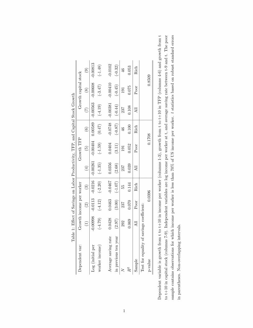
The �rst three columns in Table 1 report the OLS estimates from (12) in our three samples
when the dependent variable is the growth rate of labor productivity. Column 1 covers all
the country-years; column 2 restricts the sample to country-year pairs below 70% of US
productivity, that is, poor countries, while column 3 restricts the sample to rich countries.
In the full sample we observe some very slow convergence in income per worker. As predicted
by our model, we �nd a signi�cantly positive association between savings and productivity
growth in the ten years going forward. A more interesting prediction of our model is that
the e¤ect of savings on growth should be larger for countries far from the technology frontier
than for countries close to the frontier. This prediction is borne by the data. Comparing
11As we shall illustrate below when evaluating quantitatively the models, the horizon of interest is criticalfor the interpretation of the results.
15
the coe¢ cients of savings in columns 2 and 3 we can observe how for poor countries the
coe¢ cient of savings in the growth regression is 4.6% while for rich countries it is -4.7%.
The association between lagged average savings and productivity growth for poor countries
is statistically signi�cant while for rich countries the t-statistic is just 1.07. The di¤erence in
the coe¢ cient of savings between the two samples is statistically signi�cant at the 5 percent
level. The estimated e¤ect of lagged savings on growth in poor countries is quantitatively
important; an increase in the average saving rate between t�9 and t of 10 percentage pointsis associated with an increase in the average growth rate in output per worker of 4.6 tenths
of one percentage point over the next ten years.
Columns 4 through 6 show the robustness of the larger e¤ect of savings on growth for
poor than for rich countries to using TFP growth as dependent variable. In this case, the
coe¢ cient of savings on growth for poor countries is 4.0% while for the rich countries it
is -7.5% , a quantitatively important if not statistically signi�cant di¤erence. By contrast,
columns 7 through 9 show that there is no signi�cant e¤ect of saving on capital accumulation
in the whole sample or in either subsample. These �ndings are consistent with models such
as ours that emphasize the e¤ect of saving on technology adoption. In addition, they help
distinguish our theory from those based on the e¤ect of saving on investment through a
�nancial multiplier a la Bernanke and Gertler (1989).
It is important to note that this di¤erential e¤ect between rich and poor countries is the
opposite of what we would have expected to have resulted if measurement error was a major
issue, given that the quality of data in the Penn World Tables is generally lower for poor
countries than rich. In particular, higher measurement error in saving rates probably caused
more attenuation of its estimated e¤ect in poor countries than rich.
A related issue may arise if the savings rates are measured with more error than per
capita income levels. Since lagged savings is likely to be correlated with income at t, part
of the e¤ect of savings on growth may be captured by income. Since income should enter
negatively due to convergence and savings positively, this bias will result in lower estimates
of the e¤ect of savings and higher estimates of the e¤ect of income. (i.e. the estimated
coe¢ cient on both income and savings will be biased towards 0). This bias, however, cannot
explain our �ndings that lagged savings seems to have a stronger e¤ect on growth for poor
countries.
3.3 Robustness checks
The empirical �nding uncovered with the simple cross-country regressions is the larger co-
e¢ cient of lagged savings on growth in poor than in rich countries. This appears to be a
16
robust �nding. Table 2 shows that it also holds when using time trends or year dummies in
the estimating equation, and when including country �xed e¤ects. Table 3 shows that it is
robust to using other cuto¤s to divide the sample between poor and rich countries. We also
�nd that the regression results are robust to dropping outliers; i.e., observations more than
2 standard deviations from the regression line.
An alternative interpretation of our results is that income per capita is a proxy for �-
nancial development. According to this interpretation, �nancial development is needed to
attract foreign investment, so in �nancially less developed countries the investments under-
lying economic growth must be �nanced with domestic saving - thus saving has an e¤ect
in poor countries only because per-capita income and �nancial development are positively
correlated. To test this alternative interpretation, we split the sample not by labor produc-
tivity but by �nancial development, measured by the ratio of private credit to GDP. Our
regression tree analysis then suggested splitting the sample at the 87th percentile of �nan-
cial development. As columns 1 through 3 of Table 4 indicate, this resulted in an estimated
saving coe¢ cient that was almost the same across the two samples, in contradiction to the
alternative hypothesis. Columns 4 through 6 verify that including country �xed e¤ects does
not rescue the �nancial development hypothesis.12
4 Calibration and model evaluation
One may question using cross-country regressions to assess the importance of policies that
a¤ect saving on the dynamics of technology adoption and growth. To make further progress in
evaluating the quantitative importance of the mechanism described in our model, we calibrate
the model and conduct a Monte Carlo exercise. However, the calibration of �ve parameters
related to the process of technology adoption is not standard in the RBC literature (See
Table 1). To calibrate these new parameters we use �ve moments which ensure that the
model conforms with some basic cross-country patterns.13 Speci�cally, we can calibrate the
parameters ��; �0 and c by matching:14
� the relationship between the adoption expenditures and the proximity to the frontiera for rich countries
12Consistently with this, Comin and Nanda (2009) �nd that �nancial development a¤ects more the speedof di¤usion of new technologies for countries that are closer to the technology frontier than for countries thatare far from the frontier.13Next subsection and Appendix C provide all the details about the calibration.14Recall that these parameters denote the percent increase in the probability of success in adoption from
exerting e¤ort (��); the parameter in the cost of adopting solo (�0) and the upper bound in the distributionof the cost of e¤ort (c).
17
� the convergence dynamics for rich countries, and
� the pro�t rate in the US.
These moments contain important information. The �rst allows us to estimate how fast
adoption costs decrease with the proximity to the technology frontier. The second moment
calibrates the extent to which adoption costs a¤ect growth in rich countries. These two
moments capture elasticities of adoption costs and growth with respect to proximity, but do
not pin down the level of adoption or their costs. The third moment allows us to pin down
the level by requiring the pro�t rate of the �rms in the frontier to be consistent with the US
post-war pro�t rate.
In addition, we can calibrate the costs of adoption with a foreign investor, �; (for a given
value of �)15 from the proximity threshold at which �rms are indi¤erent between going solo
and seeking foreign help. Following Durlauf and Johnson (1995), we pin down this threshold
by conducting a regression tree analysis. The idea of this exercise is to split the sample so as
to maximize the combined R2 for the regressions run on the two subsamples. Reassuringly,
the threshold we obtain is consistent with the micro evidence that even in relatively developed
countries foreign help is often sought when adopting frontier technology.
The �nal restriction comes from several constraints that delimit the range of feasible
values of the pair (�; �). The condition that the cost of adopting solo is lower than with the
help of a foreign investor when the country is on the technology frontier, sets a lower bound
for �: The assumption that all projects that are incentive compatible are pro�table with a
foreign investor, determines an upper bound in �; for a given �. This interval of feasible
values for the pair (�; �) turns out to be quite narrow and the results are robust for the
values in the interval as well as for reasonable parametrizations outside the interval.
Next we describe in depth the calibration (deferring some details to Appendix C) and
evaluate the quantitative importance of the model to explain the dynamics of technology
adoption and the relationship between saving and growth.
4.1 Calibration
To calibrate our model we need to set values for the following parameters:
��; r; �; g; ��; �0; c; �; �
(13)
The �rst four of these parameters are common to the RBC literature and therefore we will
follow the literature when setting their values. The other �ve are not standard parameters
15Recall that � is the percentage increase in the probability of successful adoption from exerting e¤ort.
18
and we will use some "new" moments to calibrate them.
Given the OLG nature of our model, we interpret a period in the model to be 10 years.16
Following Cooley and Prescott, (1995) we set the standard parameters to the following values:
� = 1=3; r = (1:07)10 � 1; � = (1:05)10 � 1; g = (1:02)10 � 1
The value of � implies that �� = 1=3 and � = 0:074:
Since proximity a in the model is de�ned relative to the world technology frontier, we have
to take a stand on where this frontier is. We assume that the US is in the frontier. E¤ectively,
this means that, within ten years, the US adopts all the state of the art technologies.17
Regression Tree AnalysisThe threshold a has been de�ned as the relative productivity level at which a country
undertakes marginal R&D projects on its own. It therefore depends on the costs of adopting
the technology with and without a foreign investor. Information about the threshold would
help us calibrate the costs of adopting frontier technology. One approach to get such infor-
mation is to investigate the origin of technology and engineers in speci�c projects. In reality,
even for relatively rich countries, foreign consultants familiar with the frontier technology
are often involved in the adoption of frontier technology.18
We can obtain a more formal estimate of a by performing a regression tree analysis.
The idea of this exercise is to split the sample so as to maximize the combined R2 for the
regressions run on the two subsamples. We perform the analysis on the sample without the
poorest 25% of all countries and, as above, use a sample with non-overlapping intervals.
We have conducted the regression tree analysis using the baseline speci�cation in (12),
adding country �xed e¤ects or adding country random e¤ects. In all three exercises, the cut
o¤ at which countries start using the help of foreign investors to adopt frontier technolo-
gies is when output per worker is approximately below 70% of the US. (This, for example,
corresponds to Greece in 1980.) Hence, our estimate of a is 0.7.
This estimate of a is an important piece of information for our calibration for two reasons.
First, it de�nes the sample of rich countries which we use below to pin down the values of
��; �0 and c: Second, we shall use it below together with the optimal adoption decision (i.e.
eq. 6) to infer information about the adoption costs with the help of a foreign investor, �:
16Since the adoption investment is a sunk cost while output is a �ow, we interpret � and �0 as theannualized costs of adoption.17We have conducted complementary calibrations where US productivity was an additional parameter to
be estimated in the convergence regressions described below and our estimates supported this assumption.18That was, for example, the case when Siemens helped build the high speed train (AVE) in Spain in the
early 1990s.
19
R&D intensity and proximityThe fraction of sectors that try to adopt the state of the art technology in countries close
to the frontier (i.e. a > a) is given by
�(a) = v0 (1=c) =���� � ��0=a
�(1=c) :
And the share of adoption expenses in GDP is19
Adoption Expenses
GDP=
cost per project *z}|{��0=a
# of projects undertakenz}|{�(a)
a��|{z}GDP
=��0=a
a��(��� � ��0=a)
c
One reasonably good proxy for the adoption expenses for rich countries are R&D ex-
penses. Of course, there are signi�cant investments other than R&D that improve the
country�s productivity. However, it may not be unreasonable to assume that these are ap-
proximately proportional to R&D expenditures for rich countries. Under this assumption,
we can write the following non-linear relationship between R&D expenditures and proximity:�R&D
Y
�i
= �0
�1
ai
�2� �1
�1
ai
�3+ �i (14)
where �0 � ���0���c��, �1 = �0���0=��� and � captures the gap between R&D and total adoption
expenditures.
Estimating (14) for the sample of countries with ai > a in 1993 (the year for which we
have the most comprehensive R&D data), we �nd that
�0 =0:22
(0:14; 0:3)
�1 =0:11
(0:059; 0:167)
where the numbers in parenthesis are the 95 percent con�dence interval. Dividing �0 by �1;
we obtain the following restriction20
19This expression is in general an overestimate of the share of adoption expenditures. This is becausefor countries that are above a but below �a (in Figure 1), many projects are still undertaken with a foreigninvestor because this is cheaper than going solo. However, the percentage overestimation goes to zero as �increases to its upper limit (the red dashed line in Figure 2). At this limit, a and �a coincide, so all projectsare solo for countries above a. This limit actually corresponds with our baseline calibration.20Note that, the assumption on the proportionality between R&D and adoption expenditures precludes
us from using the levels of either �0 or �1 for the calibration.
20
�����0=�0
�1= 2 (15)
Convergence regressionA natural relationship to use in the calibration is the convergence equation implied by
equations (G) and (6) for the sample of high productivity countries. Using (15), this rela-
tionship can be expressed as
ln(yit+10yit
) =
�1 + g
ait�1� 1��2
�1� :5
ait�1
�+ �it;
where �2 = 2 � ����0 (1=c).Using a non-overlapping panel over the post-war period for those countries with labor
productivity higher than 70% of US level, yields the following estimate for �2;21
�2 =0:96
(0:76; 1:15)
This estimate implies that
c ' 2 � ����0 (16)
Pro�t rateWe can obtain a third restriction by using information on the US pro�t rate over the
post-war period. In particular, the pro�t rate in the model is given by
� =��� � ��0��
(17)
The average pro�t rate in the US over the post-war period has been approximately equal
to 9.5% of GDP.22 Based on this, we set � at 0.095. Plugging in the values of � and �; the
values of �0; c; � that satisfy (15), (16) and (17) are:
�0 = 0:032
c = 0:055
� = 0:85
Optimal adoptionAdopters in a country with proximity equal to a are indi¤erent between using the help
2195 percent con�dence intervals in parenthesis.22These are computed using the BEA series on corporate pro�ts with inventory valuation and capital
consumption adjustments.
21
0.1 0.2 0.3 0.4 0.5 0.6 0.7 0.8 0.9 10
0.02
0.04
0.06
0.08
0.1
0.12
delta
phi
phi>phi0
phi<phi0/0.7
phi=0.1240.0183/delta
Figure 2: Possible values of � for a given value of �:
of a foreign investor and adopting frontier technology solo.23 Formally,
v0(a) = �(v + st�1a) (18)
Setting a at 0.7, st�1 at the average (adjusted) saving rate, and �0; c; � at their calibrated
values above, yields the following relationship between � and � which is represented by the
blue curve in Figure 2:
� = 0:124� 0:0183�
(19)
This leaves just one degree of freedom in the calibration. We further restrict the set of
values for � and � by invoking two further assumptions in the model. First, � � ��0: This isrepresented by the bottom dashed line in Figure 2. Second, assumption (5) implies that24
�(v + sa) � v: (20)
Combining (18) and (20), we get that � � ��0=a = 0:045: This is represented by the top
dashed line in Figure 2. As a result, the possible values of � and � are those on the solid
23In theory, the threshold a is a function of st�1 and therefore of � : However, as we shall see below, thesteepness of v0 is such that a varies very little with � :24Recall that this assumption implied that for countries far from the frontier, all incentive compatible
projects are worthwhile.
22
curve between the two dashed lines. For example, at the upper limit where � = 0:045 we
have � = 0:23: At the lower limit, where � = 0:032; we have � = 0:20: Note that this feasible
region is fairly narrow. Since presumably � is signi�cantly larger than ��0, we set the baseline
values of � and � to 0:045 and 0:23 which are on the upper range of the region of possible
values. Our results are robust to other feasible values on the interval. Below, we also explore
the robustness of the results to relaxing the assumption that incentive compatible projects
are pro�table (i.e. eq. 20) in the calibration. Table 5 summarizes our calibrated values and
the moments used to set these values.
4.2 Model evaluation
Next, we evaluate the quantitative importance of the main mechanism described in our
model: namely, the role of domestic saving as collateral that allows countries far from the
frontier to bene�t from the knowledge of foreign investors to successfully adopt the frontier
technology. We do that in two ways. First, we compute the policy functions and the resulting
transitional dynamics to see the e¤ect of saving subsidies on saving, technology adoption and
growth. Second, we conduct a Monte Carlo exercise and estimate the same regressions we
have run in Section 3 on the simulated data to see whether the magnitude of the estimated
relationships between saving and growth for the subsamples of poor and rich countries are
comparable with the estimates we have obtained above. These exercises should provide us
with a good sense of the strength of our mechanism.
4.2.1 Policy function and transitional dynamics
Saving ratesCombining (10) and (11), we can de�ne the saving rate in our model as the value of s
that solves the following equation:25
s =
�(1� �)� �ez( 1+r1+�g
s;at�1)��(1+r)at�1
�(1� �) (21)
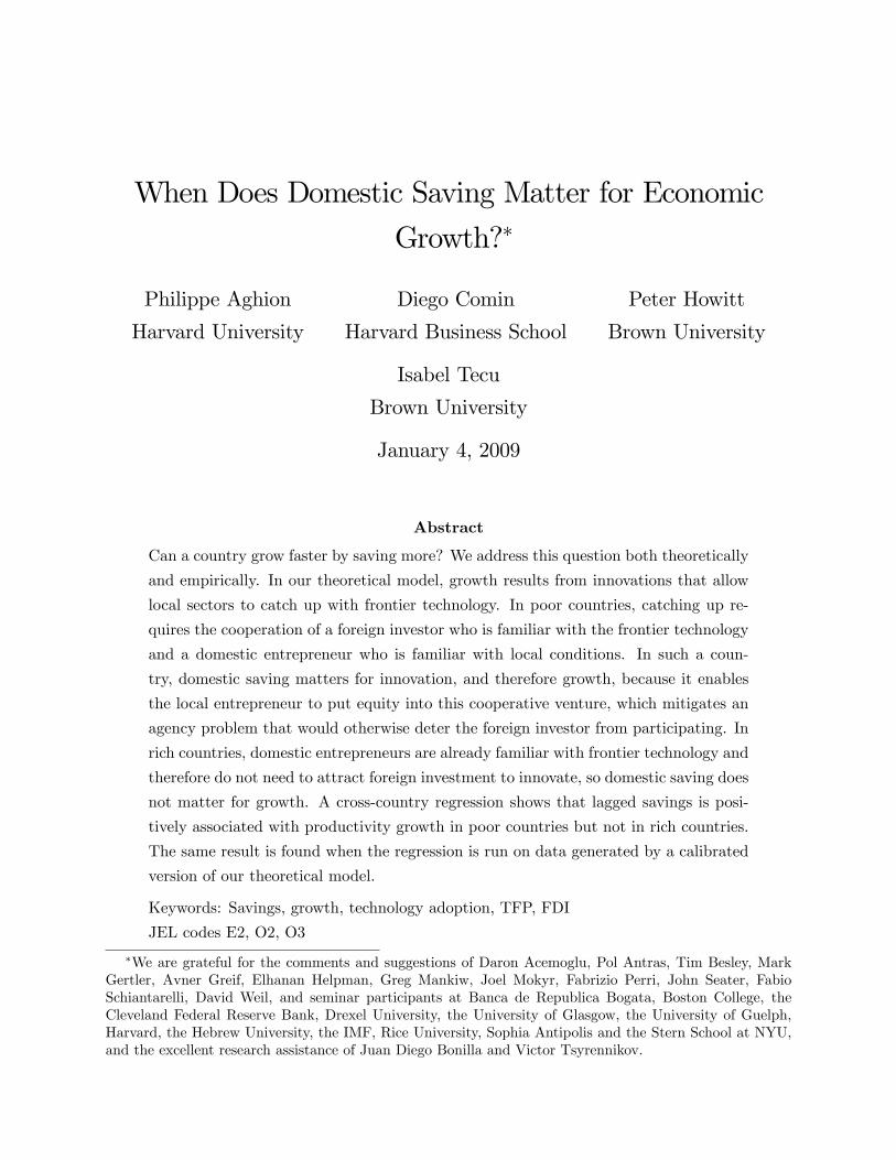
Figure 3 displays the resulting saving rate as a function of the proximity level, at�1; and
the saving subsidy, � :
25Note that this expression for the saving rate has the implicit assumption that the saving subsidies att � 1 and t are the same. This allows us to avoid the hassle of having to track down past subsidies at thesame time as identifying the subsidies in the data. It also has the advantage that we do not have to makeassumptions about the subsidies at period �1. Given the very high persistence of saving subsidies, thisseems a reasonable shortcut.
23
Figure 3: Saving rate as a function of at�1 and � :
24
The range of feasible saving rates goes from -27% to 35%. 26As one would expect, there
is a strong positive e¤ect of the saving subsidy on the saving rate. For example, for a
country with at�1 = 0:5; the saving rate goes from �1 to 33% when the saving subsidy
goes from -1 to 1. The saving rate is also increasing with the proximity to the frontier
for low initial proximity levels. This is the case because future gains from innovation are
proportional to �A while current output is proportional to At�1: As we lower at�1; the gap
between permanent income and current income increases and, as a result consumers want to
borrow more (internationally) against their future income to smooth out consumption.
Share of sectors attempting to adopt new technologiesThe share of sectors that try to adopt new technologies is given by the function �: Figure
4 plots � in terms of initial productivity and the subsidy to saving. As anticipated above, for
at�1 > a (i.e. larger than 0.7) � is independent of � and hence of savings. For lower values of
at�1; � steeply increases with the subsidy to saving. This e¤ect is quantitatively important in
our calibration. For example, for a country with a productivity level relative to the frontier
of 0.5, the share of sectors that adopt frontier technology within a period increases from 7%
to 34% as we increase the saving subsidy from the minimum to the maximum. Once the
saving rate becomes su¢ ciently large, so that �(v + s0a) > v; the incentive constraint for
projects is no longer binding and consequently � becomes independent of saving.27
GrowthTwo forces determine the growth rate of the economy. First, there is the standard
convergence e¤ect whereby a lower initial relative productivity is associated with a higher
subsequent growth. Second, for ai < a; a higher saving subsidy relaxes the incentive compat-
ibility constraint which results in a larger share of sectors adopting the frontier technology,
and therefore to faster growth. Figure 5 plots the average annual growth rate for each rel-
ative productivity and saving subsidy level. There we can see both of these mechanisms at
work. Consider, for example, two countries with saving subsidies equal to 0, but the �rst
country lies at the frontier whereas the other country is at proximity a = 0:25. The average
growth rate of the country in the frontier is 1.07% while for the country with at�1 = 0:25 it
is 5.86%. Now consider the e¤ect of the saving subsidy on growth. The average growth rate
for a country at a proximity level of 0.5 with a saving subsidy of -1 is 0.77%. By increasing
the saving subsidy to 1, the growth rate rises to 4.17%. As shown in Figure 5, the e¤ect
of the subsidy on growth is even more dramatic for poorer countries. A similar change in
the subsidy for a country with proximity 0.25 results in an increase in the growth rate from
26Though quite wide, this range does include the most extreme values of the saving rate observed in ourpanel.27Savings rates for which this happens are quite high and occur only rarely in our panel.
25
Figure 4: � as a function of at�1 and � :
26
Figure 5: Annual Growth as a function of at�1 and � :
1.85% to 8.38%.
4.2.2 Simulations
To assess the quantitative relevance of our mechanism we proceed to simulate 1000 panels,
each of which involves 140 countries and �ve periods. Two necessary inputs in this Monte
Carlo exercise are the process for the saving subsidies and the initial conditions for the
proximity levels. Inverting the saving rate plotted in Figure 3, we can �nd, for each country
and period in the data set, the saving subsidy that generates the observed saving rate given
the initial proximity level. It turns out that for 388 of the 412 country-decade observations
where initial proximity is above 0.09 (i.e. not in the bottom 25%), we can �nd interior
saving subsidies (i.e. strictly comprised between -1 and 1). The average saving subsidy is
0.03 with a median of 0.04 and a standard deviation of 0.57. As suggested by Figure A1
in Appendix C, the uniform distribution is not a bad approximation for the distribution
of saving subsidies. We therefore sample the initial subsidies from a uniform distribution
with support in [-0.96,1] to approximately match the mean and variance of the observed
27
subsidies distribution. These implied saving subsidies are quite persistent. We �nd that
their auto-correlation is 0.77. (Keep in mind that a period corresponds to 10 years.). We
use this estimate to calibrate the law of motion for subsidies in a given country. Finally, we
draw initial proximities from a Normal distribution with mean 0.3 and variance 0.0676 to
match the observed distribution of proximity levels prior to 1970.
Saving Table 6 reports basic statistics for the saving rates both in the actual (�rst row)
and simulated (second row) panels. The model does a fair job in reproducing the distribution
of saving across countries. It misses some of the very negative saving rates for which the
implied saving subsidies are binding and some of the very high saving rates observed in the
data. But the mean, median and standard deviation are very similar in the simulated and
actual data.
Saving-growth relationship Next, we reestimate the relationship between saving and
growth (12) in our Monte Carlo simulations, in a further attempt to evaluate the importance
of the mechanism described in the model. In this context, we use the Table 1 estimates from
the actual data as a benchmark.
Columns 1-3 in Table 7 reproduce the estimates from the actual data, while columns 4-6
report the average coe¢ cients (together with the 95% con�dence intervals) from the simu-
lated data. The main observation from Table 7 is that the model generates patterns of saving
and growth that are comparable to those observed in data. In particular, the estimates of
lagged saving on growth are signi�cantly larger for the poor than for the rich countries. Fur-
ther, the e¤ect of lagged saving on growth induced by our model is quantitatively important.
The average coe¢ cient for the sample of poor countries in our simulated panels is 12% with
a 95% con�dence interval of 11 to 14%. This coe¢ cient is larger than the coe¢ cient found
in the data (4.3%). As discussed in section 3, measurement error in the saving rates and the
correlation between lagged saving and current income are likely to generate a downward bias
in the estimates of the estimated e¤ect of saving on growth in the actual data. This could in
principle account for part of the discrepancy between the estimates in actual vs. simulated
data.
The average estimate of the e¤ect of saving on growth for the sample of rich countries
in our Monte Carlo exercise is zero (with a very narrow con�dence interval). Recall that in
the data, we �nd that the equivalent point estimate is statistically not di¤erent from zero.
Not surprisingly, given that a majority of countries belong to the poor-country sample, the
average estimate of the e¤ect of lagged saving on growth for the full sample in our simulations
is also quite close to the estimate in the actual data.
28
These results survive a whole set of robustness tests. First, we obtain similar estimates
of the relationship between saving and growth when calibrating � and � using other values
in the set of values that satisfy condition (20). Second, our results are robust to including
country e¤ects (both �xed and random) in the regressions. Third, the results are also robust
to relaxing the assumption that incentive compatible projects are pro�table (equation 20):
that is, to using other points along the curve in Figure 2 with � > ��0=a: Columns 7 through
9 in Table 7 present the estimates from our simulated data when calibrating � = 0:056 and
� = 0:27: We �nd that the average coe¢ cient of saving in regression (12) for the sample of
poor countries is 5.9% (rather 12%) with a 95% con�dence interval of [0.041 , 0.078]. For the
sample of rich countries, the average point estimate is still zero. Hence, the conclusion that
our model has the quantitative potential of explaining the observed patterns of saving and
growth across countries is robust to alternative choices of (�; �) in our calibration scheme.
5 Further evidence
5.1 Habit persistence
A strand of the literature on growth and saving has emphasized that the causality does not
run from saving to growth but from growth to saving. Most prominently, Carroll, Overland
and Weil (2000) have argued that if consumers are subject to internal habit formation, then
in response to an increase in their income prospects they will tend to save more in order to
avoid having to change their consumption habits in the future.
This mechanism could, in principle, be consistent with a positive short run relation
between saving and subsequent TFP growth. It is not clear though, whether this mechanism
is su¢ cient to induce a relationship as strong as the one we have estimated over the long
lags we have used in our speci�cation.
In particular, the habit model would predict a lower coe¢ cient of saving on growth when
looking at saving between t � 4 and t than when looking at more distant saving. That isnot what we have found in Aghion et al. (2006). In particular, if we look at the association
between average saving between t� 9 and t� 5 and growth (between t and t+ 10) Aghionet al. (2006) observe that the coe¢ cients are very similar to what we obtain when having as
regressor average saving between t� 9 and t or average saving between t� 4 and t.The reverse causality argument, however, may still be consistent with the insensitivity
to the lag of saving of the coe¢ cient of saving on growth if growth is very persistent. If
this was the case, future growth would be highly correlated to current growth which would
trigger very lagged saving. However, we know, at least since Easterly, Kremer, Pritchett and
29
Summers (1993), that average growth over decades presents very low autocorrelation. We
also reach a similar conclusion when estimating the e¤ect of productivity growth between
t�9 and t on productivity growth between t and t+10 after controlling for log-productivityat t.28
Finally, it is not a priori obvious that habit formation should induce a larger association
between growth and saving for poor than for rich countries as we have found in our analysis
above.
To further clarify whether habit may be causing the observed relationship between saving
and growth, we put the standard habit model to the same test as we what just did for our own
model. In particular, we take an o¤-the-shelf neoclassical growth model with habit described
in Appendix D, conduct 1000 Monte Carlo simulations on a panel of 140 countries and 50
annual observations, compute decade-long variables, estimate equation (12) and compare
the estimates with those obtained in the data and reported in Table 1.
More speci�cally, we use as dependent variables both productivity growth (Table 8) and
TFP growth (Table 9). In order to give the habit hypothesis a fair chance, we also try several
values to calibrate three parameters: the elasticity of intertemporal substitution (column 1),
the autocorrelation of the TFP shock (column 2) and the habit parameter (column 3).
Columns 4 through 6 contain the average estimate of the coe¢ cient of lagged saving on
subsequent growth and the 95% con�dence interval for the whole sample (column 4), the
sample of poor countries (column 5) and the sample of rich countries (column 6). Finally, in a
similar spirit to our evaluation of the model�s ability to reproduce some basic statistics for the
saving rate, we compare the relative volatility of investment and output in the habit model
with the data. In particular, we apply the Hodrick-Prescott �lter to each simulated annual
series and compute the ratio of the relative standard deviation of simulated investment over
the standard deviation of simulated output. Column 7 reports the average ratio across the
di¤erent simulations. In the US and other developed economies, this ratio is approximately
3, while in developing countries, it is approximately 4 (Aguiar and Gopinath, 2007). We can
use this information as a robustness check on the plausibility of the calibration.
Several observations from Tables 8 and 9 are worth noting. First, the average coe¢ cient
of lagged saving on subsequent growth for the sample of poor countries (and for the other
two samples for that matter) is almost always negative rather than positive as observed in
the regressions with actual data. Second, the con�dence intervals show that these estimates
are almost always signi�cantly smaller than zero. Third, the average coe¢ cients of lagged
saving on growth do not change much when comparing the samples of poor and rich countries
28If we do not control for log productivity at t, the autocorrelation of productivity growth can even becomenegative.
30
0 2 4 6 8 10 12 14 16 18 200
0.5
1
1.5
2
2.5
3
3.5
4
4.5
Years
Per
cent
dev
iatio
n fro
m s
tead
y st
ate
Technology Shock Impulse Response Function
technologyconsumptionoutputinvestment
Figure 6: Impulse responses to a TFP shock in a neoclassical growth model with habit.
(with the latter being more imprecise for obvious reasons).
Why is it the case that our point estimates of the association between saving and growth
are negative contrary to the intuition provided at the beginning of this section? We answer
this question with the help of Figure 6 which displays the impulse response functions of the
basic variables of the habit model to a positive technology shock.29 Basically, our answer
hinges on the horizon at which we are looking at the correlation between saving and growth.
The TFP shock a¤ects saving and investment contemporaneously and it increases growth
over the next �ve years as capital is accumulated and labor productivity increases. However,
after ten years, growth stops increasing and even starts to decline as capital depreciation
becomes larger than gross investment. Hence, when looking at the correlation between the
average saving rate over the last ten years, and growth over the next ten years, we are in
fact looking at a growth response which is either �at or negative.
Hence, the habit hypothesis is not a relevant alternative to explain the saving growth
patterns uncovered in Section 3.
29In particular, this impulse response corresponds to a calibration where the coe¢ cient of relative riskaversion is 3, habit persistence is set at 0.9 and the autocorrelation of productivity is equal to 0.99.
31
5.2 A case study: Korea in the 1960s
The Post-War growth experience in Korea has often been cited as an example where growth
led saving. Carroll, Overland and Weil (2000) have argued that growth in Korea started
during the second half of the 50s, long before the interest rate reform and the increase in
domestic private saving. Indeed, output per worker during the period 1953-58 grew at an
average annual rate of 3.8%.
This growth, however, was the result of a neoclassical catch-up process after the destruc-
tion of capital during the Korean War as well as the restoration of full capacity. During the
war (1950-53), civilian casualties approximated one million, including those killed, wounded
and missing (Bank of Korea, 1955). War damage to non-military capital and structures has
been estimated at $3.1 billion at the implicit exchange rate for 1953. The estimates of the
Korean GDP in 1953 vary substantially. As a result, the estimate of the value of non-military
assets damaged by war ranges from 86% of 1953 GNP (by the Bank of Korea) to twice GNP
(by Nathan Associates).30
It was not until 1960 that the post-war reconstruction was completed (Kim and Roemer,
1981). The end of post-war catch up coincided with a period of moderate productivity
growth which between 1958 and 1964 was 2% per year. The evolution of TFP growth is
also consistent with this interpretation. Between 1953 and 1964 TFP growth was 1.7% per
year.31 Between 1964 and 1974, labor productivity and TFP grew at annual rates of 6.2
and 3% respectively.32 In our account of the Korean experience, the reforms undertook by
Park in 1964 to control in�ation and to induce higher private saving play a critical role in
explaining this remarkable performance of TFP.
When Park took o¢ ce in 1962, Korea was emerging from the 1958-62 recession period
where in�ation had been high. In an e¤ort to reduce high in�ation the government designed
the 1965 interest rate reform on the basis of the successful experience of Taiwan�s high interest
policy during 1950-58. The Monetary Board of Korea, a committee within the central bank,
announced that the ceiling rate on saving deposits was being raised from 15% per annum
to 30% (Brown [1973], Kuznets [1977] and Kim [1991]). During the 1960-1965 the in�ation
rate was 19%. As a result, the real return on saving was negative before the interest rate
reform. In particular, in 1964 the real annual interest rate on saving accounts was -17%
(Brown, 1973). After the reform, the real interest rate on long term bank deposits rose to
11.2% in 1965.30Another estimate made by the Ministry of Commerce and Industry calculates that war damage to
manufacturing facilities was equivalent to 42 to 44 percent of pre-war facilities (Hwang, 1971).31Part of this TFP growth was surely the result of an unmeasured increase in capacity utilization and
labor hoarding when the economy went back to normal after war.32The source of the data used in these computations are the Penn World Tables and Pyo (1988).
32
The interest rate reform resulted in a rapid increase in bank saving deposits beginning in
the fourth quarter of 1965. The constant-price value of saving deposits rose by nearly 50%
in the �nal three months of 1965. The increase in interest rates raised saving both because
it increased the nominal rate and because the decline in demand reduced the in�ation rate.
Hence the e¤ect of the reform was quite persistent and the constant-price value of saving
deposits rose by 110% in 1966, and by 80% and 100% in 1967 and 1968, respectively.33
During the period 1962-66, local authorities made the �rst noticeable e¤orts to attract
foreign direct investment. These e¤orts �rst took the form of new laws allowing for tem-
porary tax holidays, or for duty-free import of machinery and raw materials approved as
investment requirements, or allowing for the remittance of principals and pro�ts and pro-
tected property against expropriation (Kuznets [1977], Kim and Roemer [1981]). In addition,
various measures aimed at promoting exports made it more attractive for foreign investors to
transfer technology (Westphal, 1978). And in those, local credit features prominently. First,
credit subsidies provided low interest loans to exporters with letters of credit from foreign
importers. These credit lines provided liquidity to producers of goods that were su¢ ciently
competitive to be exported. This helped producers provide collateral to foreign investors
who then helped producers upgrade their technology. Second, the Korean Exchange Bank
also provided suppliers�credit. Foreign suppliers of plant, equipment and raw materials to
Korean exporters provided the largest source of funds for export. Interestingly, the credits
and loans provided by these foreign suppliers were secured by the Korean Exchange Bank
(Kuznets, 1977). These credit policies in turn could be sustained thanks to the large amount
of private saving deposited in the government�s Bank in response to the interest rate reform.
These reforms surely helped solve the moral hazard problem associated with the inter-
national transfer of technology since the �ow of technology transferred to Korea increased
substantially during the period 1962-73. A �rst channel for foreign technology transfer was
foreign direct investment. In August 1962, the �rst case of a direct foreign private investment,
a US-Korea joint-venture �rm producing nylon �laments, was approved by the Government
of the Republic of Korea. In the next decade, foreign direct investment �ows increased very
fast. In 1973, the number of projects approved reached 271 and the value of foreign pri-
vate investment $262 millions (Jo, 1980). This approximately represented 16% of private
investment in Korea.
There are further considerations indicating that FDI was an active channel for foreign
technology transfer to Korea. First, FDI was directed, disproportionately, to high-tech sec-
33The post-1965 period was a period of rapid growth in Korea. Brown (1973), however, shows that theincrease in real interest rates that followed the 1965 reform had a very strong and signi�cant e¤ect on theprivate saving rate in Korea after controling for the e¤ect that private disposable income has on savings.
33
tors such as chemicals, machinery and machine parts, and specially to electric and electronic
machinery. Second, foreign-invested �rms tended to import much more than local �rms.
Third, joint-venture �rms tended to import a substantial proportion of intermediate inputs
from their foreign partner companies. Fourth, foreign-invested �rms had twice as much ma-
chinery and equipment per worker than that of local �rms and produced 80% more value
added per worker. Finally, a larger share of the output produced in foreign-invested �rms
was exported.
Another channel for foreign technology transfer was technological licensing. Jo (1980)
documents the ever-increasing trend in Korea�s technological licensing agreements with for-
eign �rms. Most of these were made with Japanese and US �rms. In 1962 only 5 agreements
were approved. In 1975, 93 new technology licensing agreements were approved, and the to-
tal royalty payments in that year amounted to almost $19 millions. As with FDI, most of the
licensing agreements were signed by �rms in high-tech sectors such as electric and electron-
ics, machinery and chemicals. This increasing adoption of foreign technologies contributed
to the high and persistent growth trend in Korea.
6 Conclusions
There are important barriers to adopting new technologies which explain the wide cross-
country di¤erences in productivity. What is the nature of these barriers, and why do some
developing countries manage to overcome them but others don�t?
This paper has developed a model where a country�s ability to take advantage of inter-
national technology di¤usion, is positively correlated with the level of its domestic savings.
Familiarity with the frontier technology reduces its cost of adoption. Advanced countries
have no problem adopting the frontier technology. However, for countries far from the tech-
nology frontier, it may be too expensive to adopt the frontier technology without outside
help. Instead, entrepreneurs in these countries need to rely on foreign investors that are
familiar with the frontier technology. However, there is moral hazard in the relationship
between local entrepreneurs and foreign investors: namely, the domestic entrepreneur may
not deliver on her input contribution, unless she has invested su¢ cient capital in the project.
This co-investment is in turn �nanced out of domestic savings. Overall, the main predic-
tion of the model is that domestic saving is more critical for adopting new technologies in
developing than in developed economies.
Confronting this predictions to available cross-country panel data, we �rst showed that
simple reduced form regressions support this basic prediction. Then, to assess the quantita-
tive importance of the above mechanism, we calibrated and simulated our model and indeed
34
found that the e¤ect of domestic saving on growth is quantitatively important. In particular,
we saw that if we restrict our sample to far-from-frontier countries, an increase in the saving
rate in the previous 10 years by 10 percentage points leads to an increase in the average
growth rate over the next 10 years of 1.3 percentage points. Moreover this e¤ect was found
to survive a whole range of robustness checks. Finally, the quantitative importance of the
e¤ect of saving on technology di¤usion over the medium term appeared to be signi�cantly
larger than the potential e¤ect of future growth on current saving operating through habit.
35
Appendix A
This appendix demonstrates that there exists a contract (x; y) satisfying conditions 1~4 in
section 2.4 of the text if and only if condition (4) holds. Suppose (4) holds. Then every
contract satis�es condition 1. Choose x = �� sa and y = x=�. By construction conditions2 and 4 are satis�ed. Also by construction we have
��� �
�(� � y)
= � (�� � �y)= � (�� � x)= � (v + sa)
so (4) implies condition 3. This establishes the if part. Now suppose that there exists a
contract (x; y) satisfying conditions 1 through 4. Conditions 2 and 3 imply
c ���� �
�(� � x=�)
which together with condition 4 and the de�nition v = �� � � implies
c � � (v + sa)
This and condition 1 imply (4). This establishes the only if part.k
Appendix B
This appendix derive the consumption function (11). De�ne X2 as the individual�s consump-
tion when old, net of the cost of entrepreneurial e¤ort:
X2 = C2 � ceAt
The utility function can be written as
u = ln (C1) +1
1 + �ln (EX2)
and the lifetime budget constraint is
(1 + �)C1 +1
1 + r(EX2 + T ) = (1 + �)wt�1 +
1
1 + rE�R� ceAt
�
36
De�ne
z � E�R� ceAt
�=At
Consider �rst the case where an individual who is given an opportunity to undertake an
investment project prefers to undertake it alone:
v � v0 (at�1)
She will realize that opportunity provided that c � v0 (at�1), so
z =
Z v0(at�1)
0
(v0 (at�1)� c) (1=c) dc:
Consider next the case where an entrepreneur would prefer to partner with a foreign
investor:
v > v0 (at�1)
She can attract a partner if and only if she has enough saving to satisfy condition (4), which
can be written using (5) as
c � ��v + s
0
t
�where we use the shorthand notation
s0t = st�1at�1
There are two subcases to consider:
1. if at�1 > ba; then by the de�nition of ba we have � (v + s0t) < v0 (at�1) andz =
Z �(v+s0t)
0
(v � c) (1=c) dc+Z v0(at�1)
�(v+s0t)
(v0 (at�1)� c) (1=c) dc
that is, if the entrepreneur�s normalized e¤ort cost c is less than � (v + s0t) then the
incentive compatibility constraint will be satis�ed and she will partner with a foreign
investor, earning an expected net rent of v � c, whereas if c is between � (v + s0t) andv0 (at�1) then although she cannot attract a foreign investor she will undertake a project
on her own, earning an expected net rent of v0 (at�1)�c. (Assumption A3 ensures thatv0 (at�1) > c:)
37
2. if at�1 � ba then v0 (at�1) � � (v + s0t) andz =
Z �(v+s0t)
0
(v � c) (1=c) dc
that is, all incentive-compatible projects with a foreigner will be undertaken but no
project will be undertaken alone.
Putting these results together we see that z can be expressed as the function
z = bz (s0t; at�1)with
@bz@s
0t
=
8><>:0 if v � v0� (v � v0) (1=c) > 0 if �
�v + s
0t
�< v0 < v
��v � �
�v + s
0t
��(1=c) > 0 if v0 � �
�v + s
0t
�9>=>;
and
@bz@at�1
=
8><>:v00v0 (1=c) > 0 if v � v0v00 (v0 � � (v + s0t)) (1=c) > 0 if � (v + s0t) < v0 < v
0 if v0 � � (v + s0t)
9>=>;where we have suppressed the argument at�1 of the v0 function.
Equivalently we can use the de�nition of s0t to write
z = ez (st�1; at�1)where ez is de�ned as ez (st�1; at�1) = bz (st�1at�1; at�1)which the above results show is increasing in both arguments.
The young individual�s problem is therefore
maxfC1;EX2g
ln (C1) +11+�
ln (EX2)
subj to (1 + �)C1 +11+rEX2 = W + 1
1+rAtez � (1+r)(wt�1�C1)at�1At
; at�1
�where W = (1 + �)wt�1 � 1
1+rT . The �rst-order conditions for this problem together with
the government budget constraint (9) yield (11).k
38
Appendix C
In this appendix we expand on some of the calibration details not included in section 4.1.
Mechanics of the regression tree analysis
For each year, we compute the gap in log GDP per worker between country i and the
US. For each integer n between 1 and 98, we then perform the following steps:
1. Split the sample into two subsamples, one with log GDP per worker gap above the
nth percentile (the �rich�sample) and one with the log GDP per worker gap at or below the
nth percentile (the �poor�sample).
2. Regress growth in TFP between year t and year t + 10 on log GDP per worker in
year t and average saving over the years t� 9 to t on the poor sample and the rich sampleseparately. In our baseline speci�cation we conduct this exercise without any country e¤ect,
but we test the robustness of the results to including country �xed e¤ect and random e¤ects.
3. For each of the two regressions, compute the sum of squared residuals (SSR) and add
them together.
We then select n� as the n for which the SSR is lowest. Splitting the sample along the
n�th percentile of the log GDP per worker gap therefore results in two samples for which
both regressions together have the highest explanatory power. As mentioned in the text,
we conduct this exercise using the baseline speci�cation in (12), adding country �xed e¤ects
and adding country random e¤ects. In all three exercises, n� is the 88th percentile. This
correspond to a level in per worker output relative to the US of 0.7.
39
0.2
.4.6
.8D
ensi
ty
1 .5 0 .5 1tau
Figure A1: Distribution of savings subsidies (�).
Appendix D
This appendix describes the habit model used to explore the reverse causality hypothesis
that future growth prospects drive lagged saving. A period is calibrated to a year. Before
running the regressions, we compute decade-long growth rates and average saving rates to
match the analysis conducted with the actual data and the data simulated from our model.
The lifetime utility of the representative consumer is
U =1Xt=0
�t(ct � hct�1)1��
1� �
where � is the coe¢ cient of risk aversion, h is the habit persistence parameter, and
� = 0:95 is the discount factor. labor supply is exogenous.
Production is done according to the following Cobb-Douglas function
Yt = AtK�t L
1��;
with � = 1=3; and the log of At follows an AR(1) with an exogenous drift that generates
40
steady state growth in labor productivity of 2 percent per year and the annual standard
deviation of the innovations to TFP are set to 2 percent. The depreciation rate is set to 8
percent per year.
41
References
[1] Aghion, Philippe, Diego Comin and Peter Howitt. "When Does Domestic Saving Matter
for Economic Growth?" NBER Working Paper No. 12275 (May 2006).
[2] Aguiar, Mark and Gita Gopinath, 2007. "Emerging Market Business Cycles: The Cycle
Is the Trend," Journal of Political Economy, University of Chicago Press, vol. 115
(2007): 69-102.
[3] Alfaro, Laura and Sebnem Kalemli-Ozcan and Vadym Volosovych, 2008. "Why Doesn�t
Capital Flow from Rich to Poor Countries? An Empirical Investigation," The Review
of Economics and Statistics, MIT Press, vol. 90(2), (2008): 347-368.
[4] Alfaro, Laura, Areendam Chanda, Sebnem Kalemli-Ozcan, and Selin Sayek. "FDI and
Economic Growth: The Role of Local Financial Markets." Journal of International
Economics 64, (2004): 89-112.
[5] Antras, Pol, Mihir Desai, and C. Fritz Foley. "Multinational Firms, FDI Flows and
Imperfect Capital Markets." Quarterly Journal of Economics 124 (2009): forthcoming.
[6] Attanasio, Orazio P., Lucio Picci and Antonello E. Scorcu. "Saving, Growth, and In-
vestment: A Macroeconomic Analysis Using a Panel of Countries," The Review of Eco-
nomics and Statistics, MIT Press, vol. 82(2), (2000): 182-211
[7] Banerjee, Abhijit V. and Du�o, Esther. "Growth Theory through the Lens of Devel-
opment Economics," in Handbook of Economic Growth edited by Philippe Aghion and