Zero-knowledge proof systems for QMA

Anne Broadbent1 Zhengfeng Ji2,3 Fang Song4 John Watrous5,6

1Department of Mathematics and StatisticsUniversity of Ottawa, Canada

2Centre for Quantum Computation and Intelligent Systems, School of SoftwareFaculty of Engineering and Information Technology

University of Technology Sydney, Australia3State Key Laboratory of Computer Science, Institute of Software

Chinese Academy of Sciences, China4Institute for Quantum Computing and Department of Combinatorics & Optimization

University of Waterloo, Canada5Institute for Quantum Computing and School of Computer Science

University of Waterloo, Canada6Canadian Institute for Advanced Research

Toronto, Canada

April 12, 2016

Abstract

Prior work has established that all problems in NP admit classical zero-knowledge proofsystems, and under reasonable hardness assumptions for quantum computations, these proofsystems can be made secure against quantum attacks. We prove a result representing a furtherquantum generalization of this fact, which is that every problem in the complexity class QMAhas a quantum zero-knowledge proof system. More specifically, assuming the existence of anunconditionally binding and quantum computationally concealing commitment scheme, weprove that every problem in the complexity class QMA has a quantum interactive proof systemthat is zero-knowledge with respect to efficient quantum computations.

Our QMA proof system is sound against arbitrary quantum provers, but only requires anhonest prover to perform polynomial-time quantum computations, provided that it holds aquantum witness for a given instance of the QMA problem under consideration. The proofsystem relies on a new variant of the QMA-complete local Hamiltonian problem in which thelocal terms are described by Clifford operations and standard basis measurements. We believethat the QMA-completeness of this problem may have other uses in quantum complexity.

arX

iv:1

604.

0280

4v1

[qu

ant-

ph]

11

Apr

201

6

1 Introduction

Zero-knowledge proof systems, first introduced by Goldwasser, Micali and Rackoff [23], are in-teractive protocols that allow a prover to convince a verifier of the validity of a statement whilerevealing no additional information beyond the statement’s validity. Although paradoxical as itappears, several problems that are not known to be efficiently computable, such as the QuadraticNon-Residuosity, Graph Isomorphism, and Graph Non-Isomorphism problems, were shown toadmit zero-knowledge proof systems [21, 23]. Under reasonable intractability assumptions, Gol-dreich, Micali and Wigderson [21] gave a zero-knowledge protocol for the Graph 3-Coloring prob-lem and, because of its NP-completeness, for all NP problems. This line of work was further ex-tended in [7], which showed that all problems in IP have zero-knowledge proof systems.

Since the invention of this concept, zero-knowledge proof systems have become a cornerstoneof modern theoretical cryptography. In addition to the conceptual innovation of formulating acomplexity-theoretic notion of knowledge, zero-knowledge proof systems are essential buildingblocks in a host of cryptographic constructions. One notable example is the design of secure two-party and multi-party computation protocols [20].

The extensive works on zero-knowledge largely reside in a classical world. The developmentof quantum information science and technology has urged another look at the landscape of zero-knowledge proof systems in a quantum world. Namely, both honest users and adversaries maypotentially possess the capability to exchange and process quantum information. There are, ofcourse, zero-knowledge protocols that immediately become insecure in the presence of quantumattacks due to efficient quantum algorithms that break the intractability assumptions upon whichthese protocols rely. For instance, Shor’s quantum algorithms for factoring and computing dis-crete logarithms [42] invalidate the use of these problems, generally conjectured to be classicallyhard, as a basis for the security of zero-knowledge protocols against quantum attacks. Even withcomputational assumptions against quantum adversaries, however, it is still highly nontrivial toestablish the security of classical zero-knowledge proof systems in the presence of malicious quan-tum verifiers because of a technical reason that we now briefly explain.

The zero-knowledge property of a proof system for a fixed input string is concerned with thecomputations that may be realized through an interaction between a (possibly malicious) verifierand the prover. That is, the malicious verifier may take an arbitrary input (usually called the auxil-iary input to distinguish it from the input string to the proof system under consideration), interactwith the prover in any way it sees fit, and produce an output that is representative of what it haslearned through the interaction. Roughly speaking, the prover is said to be zero-knowledge on thefixed input string if any computation of the sort just described can be efficiently approximated1

by a simulator operating entirely on its own—meaning that it does not interact with the prover,and in the case of an NP problem it does not possess a witness for the fixed problem instancebeing considered. The proof system is then said to be zero-knowledge when this zero-knowledgeproperty holds for all yes-instances of the problem under consideration.

Classically speaking, the zero-knowledge property is typically established through a tech-nique known as rewinding. In essence, the simulator can store a copy of its auxiliary input, andit can make guesses and store intermediate states representing a hypothetical prover/verifierinteraction—and if it makes a bad guess or otherwise experiences bad luck when simulating thishypothetical interaction, it simply reverts to an earlier stage (or possibly back to the beginning)

1 Different notions of approximations are considered, including statistical approximations and computational ap-proximations, which require that the simulator’s computation is either statistically (or information-theoretically) indis-tinguishable or computationally indistinguishable from the malicious verifier’s computation. This paper is primarilyconcerned with the computational variant.

1

of the simulation and tries again. Indeed, it is generally the simulator’s freedom to disregard thetemporal restrictions of the actual prover/verifier interaction in a way such as this that makes itpossible to succeed.

However, rewinding a quantum simulation is more problematic; the no-cloning theorem [51] for-bids one from copying quantum information, making it impossible to store a copy of the input orof an intermediate state, and measurements generally have an irreversible effect [16] that may par-tially destroy quantum information. Such difficulties were first observed by van de Graaf [45] andfurther studied in [11, 46]. Later, a quantum rewinding technique was found [49] to establish thatseveral interactive proof systems, including the Goldreich-Micali-Wigderson Graph 3-Coloringproof system [21], remain zero-knowledge against malicious quantum verifiers (under appro-priate quantum intractability assumptions in some cases). It follows that all NP problems havezero-knowledge proof systems even against quantum malicious verifiers, provided that a quan-tum analogue of the intractability assumption required by the Goldreich-Micali-Wigderson Graph3-Coloring proof system are in place.

This work studies the quantum analogue of NP, known as QMA, in the context of zero-knowledge. These are problems with a succinct quantum witness satisfying similar completenessand soundness to NP (or its randomized variant MA). Quantum witnesses and verification areconjectured to be more powerful than their classical counterparts: there are problems that admitshort quantum witnesses, whereas there is no known method for verification using a polynomial-sized classical witness. In other words, NP ⊆ QMA holds trivially, and the containment is typi-cally conjectured to be proper. The question we address in this paper is: Does every problem in QMAhave a zero-knowledge quantum interactive proof system? In more philosophical terms, viewing quan-tum witnesses as precious sources of knowledge: Can one always devise a proof system that revealsnothing about a quantum witness beyond its validity?

1.1 Our contributions

We answer the above question positively by constructing a quantum interactive proof system forany problem in QMA that is zero-knowledge against any polynomial-time quantum adversary,under a reasonable quantum intractability assumption.

Theorem 1. Assuming the existence of an unconditionally binding and quantum computationally conceal-ing bit commitment scheme, every problem in QMA has a quantum computational zero-knowledge proofsystem.

A few of the desirable features of our proof system are as follows:

1. Our proof system has a simple structure, similar to the classical Goldreich-Micali-WigdersonGraph 3-Coloring proof system (and to the so-called Σ-protocols more generally). It can beviewed as a three-phase process: the prover commits to a quantum witness, the verifier makesa random challenge, and finally the prover responds to the challenge by partial opening of thecommitted information that suffices to certify the validity.

2. All communications in our proof system are classical except for the first commitment message,and the verifier can measure the quantum message immediately upon its arrival (which has astrong technological appeal).

3. Our protocol is based on mild computational assumptions. The sort of bit commitment schemeit requires can be implemented, for instance, under the existence of injective one-way functionsthat are hard to invert in quantum polynomial time.

2

4. Our protocol is prover-efficient. It is sound against general quantum provers, but given a validquantum witness, an honest prover only needs to perform efficient quantum computations.As has already been suggested, aside from the preparation of the first quantum message, allof the remaining computations performed by the honest prover are classical polynomial-timecomputations.

As a key ingredient of our zero-knowledge proof system, we introduce a new variant of thek-local Hamiltonian problem and prove that it remains QMA-complete (with respect to Karp re-ductions). The k-local Hamiltonian problem asks if the minimum eigenvalue (or ground state en-ergy in physics parlance) of an n-qubit Hamiltonian H = ∑j Hj, where each Hj is k-local (i.e.,acts trivially on all but k of the n qubits), is below a particular threshold value. This problem wasintroduced and proved to be QMA-complete (for the case k = 5) by Kitaev [34]. We show thateach Hj can be restricted to be realized by a Clifford operation, followed by a standard basis mea-surement, and the QMA-completeness is preserved. Beyond its use in this paper, this fact has thepotential to provide other insights into the study of quantum Hamiltonian complexity. For an ar-bitrary problem A ∈ QMA, we can reduce an instance of A efficiently to an instance of the k-localClifford Hamiltonian problem, and a valid witness for A can also be transformed into a witnessfor the corresponding k-local Clifford Hamiltonian problem instance by an efficient quantum pro-cedure. As a result, A has a zero-knowledge proof system by composing this reduction with ourzero-knowledge proof system for the k-local Clifford Hamiltonian problem.

Our proof system also employs a new encoding scheme for quantum states, which we con-struct by extending the trap scheme proposed in [10]. While our new scheme can be seen as aquantum authentication scheme (cf. [2, 5, 6]), it in addition allows performing arbitrary constant-qubit Clifford circuits and measuring in the computational basis directly on authenticated datawithout the need for auxiliary states. Previously the only known scheme supporting this featurerequires high-dimensional quantum systems (i.e., qudits rather than qubits) [6], which make itinconvenient in our setting where all quantum operations are on qubits.

1.2 Overview of protocol and techniques

A natural approach to constructing zero-knowledge proofs for QMA is to consider a quantumanalogue of the Goldreich-Micali-Wigderson proof system for Graph 3-Coloring (which we willhereafter refer to as the GMW 3-Coloring proof system). Let us focus in particular on the localHamiltonian problem, and consider a proof system in which the prover holds a quantum witnessstate for an instance of this problem, commits to this witness, and receives the challenge from theverifier (which, let us say, is a random term of the local Hamiltonian). The prover might then openthe commitments of the set of qubits on which the term acts non-trivially so that the verifier canmeasure the local energy for this term and determine acceptance accordingly.

There is a major difficulty when one attempts to carry out such an approach for QMA. Thezero-knowledge property of the GMW 3-Coloring proof system depends crucially on a structuralproperty of the problem: the honest prover is free to randomize the three colors used in its coloring,and when the commitments to the colors of two neighboring vertices are revealed, the verifierwill see just a uniform mixture over all pairs of different colors. This uniformity of the coloringmarginals is important in achieving the zero-knowledge property of the proof system. Unlike thecase of 3-Coloring, however, none of the known QMA-complete problems under Karp reductionshas such desirable properties. For example, if we use local Hamiltonian problems directly in aGMW-type proof system, of the sort suggested above, information about the reduced state of thequantum witness will be leaked to the verifier, possibly violating the zero-knowledge requirement.

3

To overcome the difficulty suggested above, we employ several ideas that enable the prover to“partially” open the commitments, revealing only the fact that the committed state lives in certainsubspaces, and nothing further. Our first technique simplifies the verification circuit for QMA-complete problems through the introduction of the local Clifford-Hamiltonian problem that wasalready described. Somewhat more specifically, our formulation of this problem requires everyHamiltonian term to take the form C∗|0k〉〈0k|C for some Clifford operation C. Because the localClifford-Hamiltonian problem remains QMA-complete, it implies a random Clifford verificationprocedure for problems in QMA: intuitively, the verification of a quantum witness has been sim-plified to a Clifford measurement followed by a classical verification.

The Clifford verification procedure works in harmony with the encryption of quantum data viathe quantum one-time pad and other derived hybrid schemes that are used by our proof system.This has the important effect of transforming statements about quantum states into those aboutthe classical keys of the quantum one-time pad, which naturally leads to our second main idea:the use of zero-knowledge proofs for NP against quantum attacks to simplify the construction ofzero-knowledge proofs for QMA. In our protocol, the verifier measures the encrypted quantumdata and asks the prover to prove, using a zero-knowledge protocol for NP, that the decryption ofthis result is consistent with the verifier accepting.

In fact, if the verifier measures the quantum data according to the specifications of the protocol,the combination of the Clifford verification and the use of zero-knowledge proofs for NP suffices.A problem arises, however, if the verifier does not perform the honest measurement. Our thirdtechnique, inspired by work on quantum authentication [2, 6, 10, 14], employs a new scheme forencoding quantum states. Roughly speaking, if the prover encodes a witness state under our en-coding scheme, then the verifier is essentially forced to perform the measurement honestly—anyattempt to fake a “logically different” measurement result will succeed with negligible probabil-ity. In our proof system, we adapt the trap scheme proposed in [10] so that we can perform anyconstant-sized Clifford operations on authenticated quantum data followed by computational ba-sis measurements, benefiting along the way from ideas concerning quantum computation on au-thenticated quantum data.

The resulting zero-knowledge proof system for QMA has a similar overall structure to theGMW 3-Coloring protocol: the prover encodes the quantum witness state using a quantum au-thentication scheme, and sends the encoded quantum data together with a commitment to thesecret keys of the authentication to the verifier. The verifier randomly samples a term C∗|0k〉〈0k|Cin the local Clifford-Hamiltonian problem, applies the operation C transversally on the encodedquantum data and measures all qubits corresponding to the k qubits of the selected term in thecomputational basis, and sends the measurement outcomes to the prover. The prover and verifierthen invoke a quantum-secure zero-knowledge proof for the NP statement that the commitmentcorrectly encodes an authentication key and, under this key, the verifier’s measurement outcomesdo not decode to 0k.

1.3 Comparisons to related work

There has been other work on quantum complexity and theoretical cryptography, some of whichis discussed below, that allows one to conclude statements having some similarity to our results.We will argue, however, that with respect to the problem of devising zero-knowledge quantuminteractive proof systems for QMA, our main result is stronger in almost all respects. In addition,we believe that our proof system is appealing both because it is conceptually simple and representsa natural extension of well-known classical methods.

4

1. Zero-knowledge proof systems for all of IP. Hallgren, Kolla, Sen and Zhang [27] proved that clas-sical zero-knowledge proof systems for IP [7] can be made secure against malicious quantumverifiers under a certain technical condition. It appears that this condition holds assuming theexistence of a quantum computationally hiding commitment scheme. Because QMA is con-tained in IP, this would imply a classical zero-knowledge protocol for QMA. However, thisgeneric protocol would require a computationally unbounded prover to carry out the honestprotocol, and it is unlikely to reduce the round complexity without causing unexpected conse-quences in complexity theory [22, 24, 47].

2. Secure two-party computations. Another approach to constructing zero-knowledge proofs forQMA is to apply the general tool of secure two-party quantum computation [6, 13, 14]. In par-ticular, we may imagine two parties, a prover and a verifier, jointly evaluating the verificationcircuit of a QMA problem, with the prover holding a quantum witness as his/her private in-put. In principle, one can design a two-party computation protocol so that the verifier learnsthe validity of the statement but nothing more about the prover’s private input. While we be-lieve that a careful analysis could make this approach work, it comes at a steep cost. First, weneed to make significantly stronger computational assumptions, as secure quantum two-partycomputation relies on (at least) secure computations of classical functions against quantum ad-versaries. The best-known quantum-secure protocols for classical two-party computation as-sume quantum-secure dense public-key encryption [28] or similar primitives [36], in contrastto the existence of a quantum computationally hiding commitment scheme.2 Secondly, the pro-tocol obtained this way is only an argument system. That is, the protocol is only sound againstcomputationally bounded dishonest provers. Moreover, the generic quantum two-party com-putation protocol evaluates the verification circuit gate by gate, and in particular interactionsare unavoidable for some (non-Clifford) gates. This causes the round complexity to grow inproportion to the size of the verification circuit. In addition, the communications are inherentlyquantum, which makes the protocol much more demanding from a technological viewpoint.

On the positive side, through this approach, it is possible to achieve negligible soundness er-ror using just one copy of witness state. In contrast, our proof system directly inherits thesoundness error of the most natural and direct verification for the local Clifford-Hamiltonianproblem (i.e., randomly select a Hamiltonian term and measure). If one reduces an arbitraryQMA-verification procedure to an instance of this problem, the resulting soundness guaranteecould be significantly worse.

3. Zero-knowledge proofs for Density Matrix Consistency. It was pointed out by Liu [35] that theDensity Matrix Consistency problem, which asks if there exists a global state of n qubits thatis consistent with a collection of k-qubit density matrix marginals, should admit a simple zero-knowledge proof system following the GMW 3-Coloring approach. This fact was one of theinspirations for our work. While it approaches our main result, it does not necessarily admita zero-knowledge proof system for all problems in QMA, as the Density Matrix Consistencyproblem is only known to be hard for QMA with respect to Cook reductions.

4. Other results on Clifford verifications for QMA. We note that Clifford verification with classicalpost-processing of QMA was considered in [38] using magic states as ancillary resources. Ourconstruction is arguably simpler, uses only constant-size Clifford operations, and most impor-tantly does not require any resource states. This helps to avoid checking the correctness ofresource states in the final zero-knowledge protocol. We are hopeful that our techniques will

2 Roughly speaking, this distinction is analogous to “Cryptomania” vs “minicrypt” according to Impagliazzo’s five-world paradigm [30].

5

provide new insights to the study of quantum Hamiltonian complexity, and may find usefulapplications in other areas of research such as the study of non-local games. One byproduct ofour Clifford-Hamiltonian reduction proof is an alternative proof of the single-qubit measure-ment verification for QMA recently proposed by [39].

Organization

The remainder of the paper is organized as follows. Section 2 describes the variant of the localHamiltonian problem mentioned above. We present our zero-knowledge proof system for QMAin Section 3 and prove its completeness and soundness in Section 4 and zero-knowledge propertyin Section 5. We conclude with some remarks and future directions in Section 6. An appendixsummarizing basic notation, definitions, and useful primitives for the construction of our zero-knowledge proof system is also included for completeness.

2 The local Clifford-Hamiltonian problem

The local Hamiltonian problem [34] is a well-known example of a complete problem for QMA,provided that certain assumptions are in place regarding the gap between the ground state en-ergy (i.e., the smallest eigenvalue) of input Hamiltonians for yes- and no-inputs. A general andsomewhat imprecise formulation of the local Hamiltonian problem is as follows.

The k-local Hamiltonian problem (k-LH)

Input: A collection H1, . . . , Hm of k-local Hamiltonian operators, each acting on n qubits andsatisfying 0 ≤ Hj ≤ 1 for j = 1, . . . , m, along with real numbers α and β satisfying α < β.

Yes: There exists an n-qubit state ρ such that 〈ρ, H1 + · · ·+ Hm〉 ≤ α.

No: For every n-qubit state ρ, it holds that 〈ρ, H1 + · · ·+ Hm〉 ≥ β.

This problem statement is imprecise in the sense that it does not specify how α and β are to berepresented or what requirements are placed on the gap β− α mentioned above. We will be moreprecise about these issues when formulating a restricted version of this problem below, but it isappropriate that we first summarize what is already known.

It is known that k-LH is complete for QMA (with respect to Karp reductions) provided α andβ are input in a reasonable way and separated by an inverse polynomial gap; this was first provedby Kitaev [34] for the case k = 5, then by Kempe and Regev [32] for k = 3 and Kempe, Kitaev, andRegev [31] for k = 2. If one adds the additional requirement that α is exponentially small, whichwill be important in the context of this paper, then QMA-completeness for k = 5 still follows fromKitaev’s proof, but the proofs of Kempe and Regev and Kempe, Kitaev, and Regev do not implythe same for k = 3 and k = 2. On the other hand, the work of Bravyi [9] and Gosset and Nagaj [25]does establish QMA-completeness for exponentially small α, for k = 4 and k = 3, respectively.

The restricted version of the local Hamiltonian we introduce is one in which each Hamiltonianterm Hj is not only k-local and satisfies 0 ≤ Hj ≤ 1, but furthermore on the k qubits on which itacts nontrivially, its action must be given by a rank 1 projection operator of the form

C∗j |0k〉〈0k|Cj, (1)

for some choice of a k-qubit Clifford operation Cj. For brevity, we will refer to any such operator asa k-local Clifford-Hamiltonian projection. The precise statement of our problem variant is as follows.

6

The k-local Clifford-Hamiltonian problem (k-LCH)

Input: A collection H1, . . . , Hm of k-local Clifford-Hamiltonian projections, along with positiveintegers p and q expressed in unary notation (i.e., as strings 1p and 1q) and satisfying2p > q.

Yes: There exists an n-qubit state ρ such that 〈ρ, H1 + · · ·+ Hm〉 ≤ 2−p.

No: For every n-qubit state ρ, it holds that 〈ρ, H1 + · · ·+ Hm〉 ≥ 1/q.

It may be noted that, by the particular way we have stated this problem, we are focusing on avariant of the local Hamiltonian problem in which the parameter α may be exponentially smalland the gap β− α is at least inverse polynomial.

Theorem 2. The 5-local Clifford-Hamiltonian problem is QMA-complete with respect to Karp reductions.Moreover, for any choice of promise problem A = (Ayes, Ano) ∈ QMA and a polynomially boundedfunction p, there exists a Karp reduction f from A to 5-LCH having the form

f (x) =⟨

H1, . . . , Hm, 1p(|x|), 1q⟩

(2)

for every x ∈ Ayes ∪ Ano.

Proof. The containment of the 5-local Clifford-Hamiltonian problem in QMA follows from thefact that the 5-LH problem is in QMA for the same choice of the ground state energy bounds. Ittherefore remains to prove the statement concerning the QMA-hardness of the 5-LCH problem.

Let A = (Ayes, Ano) be any promise problem in QMA and let p be a polynomially boundedfunction. Using a standard error reduction procedure for QMA, one may conclude that there existsa polynomial-time generated collection Vx : x ∈ Ayes ∪ Ano of measurement circuits havingthese properties:

1. If x ∈ Ayes, there exists a state ρ such that Vx(ρ) = 1 with probability 1− 2−p(|x|).

2. If x ∈ Ano, then for all quantum states ρ representing valid inputs to Vx it holds that Vx(ρ) = 1with probability at most 1/2.

It is known that Λ(P), H is a universal gate set for quantum computation, so there wouldbe no loss of generality in assuming each Vx is a quantum circuit using gates from this set, to-gether with a supply of ancillary qubits initialized to the state |0〉. For technical reasons (which arediscussed later) we will assume something marginally stronger, which is that each Vx uses gatesfrom the set Λ(P), H⊗ H. That is, every Hadamard gate appearing in Vx is paired with anotherHadamard gate to be applied at the same time but on a different qubit. Note that for any circuitcomposed of gates from the set Λ(P), H, this stronger condition is easily met by adding to thiscircuit a number of additional Hadamard gates on an otherwise unused ancilla qubit.

Now consider the 5-local circuit-to-Hamiltonian construction of Kitaev [34], for a given choiceof Vx. In this construction, the resulting Hamiltonians have the form

Htotal = Hin + Hout + Hclock + Hprop, (3)

where the terms check the initialization, readout, validity of unary clock, and propagation of com-putation respectively. It follows from Kitaev’s proof that, for x ∈ Ayes, the resulting HamiltonianHtotal has ground state energy at most 2−p(|x|), and for x ∈ Ano the ground state energy of Htotal isat least 1/q(|x|), for some polynomially bounded function q. To complete the proof, it suffices to

7

demonstrate that each of these terms can be expressed as a sum of Clifford-Hamiltonian projec-tions.

The first three terms, Hin, Hout, and Hclock, can be expressed as sums of Clifford-Hamiltonianprojections easily, as they are all projection operators that are diagonal in the standard basis. Thepropagation term has the form Hprop = ∑T

t=1 Hprop,t where each operator Hprop,t takes the form

Hprop,t =12[(|100〉〈100|t−1,t,t+1 + |110〉〈110|t−1,t,t+1)⊗ 1

− |110〉〈100|t−1,t,t+1 ⊗Ut − |100〉〈110|t−1,t,t+1 ⊗U∗t]

= |10〉〈10|t−1,t+1 ⊗12[1t ⊗ 1− |1〉〈0|t ⊗Ut − |0〉〈1|t ⊗U∗t

].

(4)

Here, the first three qubits (indexed by t − 1, t, and t + 1) refer to qubits in a clock register andUt represents the t-th unitary gate in Vx. To prove that each propagation operator Hprop,t can beexpressed as a sum of Clifford-Hamiltonian projections, it suffices to prove the same for everyprojection of the form

12[1⊗ 1− |1〉〈0| ⊗U − |0〉〈1| ⊗U∗

], (5)

for U being either Λ(P) or H ⊗ H.In the case that U = Λ(P), one has that the projection (5) is the sum of the four Clifford-

Hamiltonian projections corresponding to these vectors:

|−〉|00〉 = (ZH ⊗ 1⊗ 1)|000〉,|−〉|01〉 = (ZH ⊗ 1⊗ X)|000〉,|−〉|10〉 = (ZH ⊗ X⊗ 1)|000〉,|〉|11〉 = (P∗H ⊗ X⊗ X)|000〉,

(6)

where |〉 = (|0〉 − i|1〉)/√

2. In the case that U = H ⊗ H, one has that the projection (5) is thesum of the four Clifford-Hamiltonian projections corresponding to these vectors:

|ψ1〉 =(|000〉 − |011〉 − |101〉 − |110〉

)/2,

|ψ2〉 =(|000〉+ |011〉 − |100〉 − |111〉

)/2,

|ψ3〉 =(|001〉 − |010〉+ |101〉 − |110〉

)/2,

|ψ4〉 =(|001〉+ |010〉 − |100〉+ |111〉

)/2.

(7)

All four of these vectors are obtained by a Clifford operation applied to the all-zero state. In par-ticular, when the following Clifford circuits are applied to the state |000〉, the states |ψ1〉, |ψ2〉, |ψ3〉,and |ψ4〉 are obtained:

H

H

Z

Z H

H

Z H

H

X

Z

H

H

Z

Z

X

This completes the proof.

Remark 1. If one is given a witness to a given QMA problem A, it is possible to efficiently computea witness to the corresponding k-local Hamiltonian problem instance through Kitaev’s reduction.Our reduction also inherits this property.

8

Remark 2. There is no loss of generality in setting q = 1 in the statement of the k-LCH prob-lem, meaning that Theorem 2 holds for this somewhat simplified problem statement. This may beproved by repeating each Hamiltonian term q times in a given problem instance and adjusting pas necessary.

Remark 3. States of the form C|0k〉, for a Clifford operation C, are stabilizer states of k qubits.Theorem 2 therefore implies that there exists a QMA verification procedure in which the veri-fier randomly chooses a k-qubit stabilizer state and checks whether the quantum witness state isorthogonal to it.

Remark 4. If one takes U = H in (5), the resulting projection operator projects onto the two-dimensional subspace spanned by the vectors |−〉|γ0〉 and |+〉|γ1〉, where

|γ0〉 = cos(π/8)|0〉+ sin(π/8)|1〉 and |γ1〉 = sin(π/8)|0〉 − cos(π/8)|1〉 (8)

are eigenvectors of H. This projection cannot be expressed as a sum of Clifford-Hamiltonian pro-jections, which explains why we needed to replace H with H ⊗ H in the proof above.

While considering this projection is not useful for proving Theorem 2, we do obtain from ita different result. In particular, we obtain an alternative proof of a result due to Morimae, Nagaj,and Schuch [39] establishing that single-qubit measurements and classical post-processing are suf-ficient for QMA verification. Reference [39] actually provides two proofs of this fact, one based onmeasurement-based quantum computation and the other based on a local-Hamiltonian problemtype of approach similar to what we propose. While their local-Hamiltonian approach does notwork for one-sided error (or QMA1) verifications, ours does (as does their measurement-basedquantum computation proof).

3 Description of the proof system

In this section we describe our zero-knowledge proof system for the local Clifford-Hamiltonianproblem. The main steps of the proof system are described in the subsections that follow, and theentire proof system is summarized in Figure 1. Properties of the proof system, including complete-ness, soundness, and the zero-knowledge property, are discussed in later sections of the paper.

As suggested previously, our proof system makes use of a bit commitment scheme, and inthe interest of simplicity in explaining and analyzing the proof system we shall assume that thisscheme is non-interactive. One could, however, replace this non-interactive commitment schemeby a different scheme (such as Naor’s scheme with a 1-round commitment phase [40]). Through-out this section it is to be assumed that an instance of the k-local Clifford-Hamiltonian problem hasbeen selected. The instance describes Clifford-Hamiltonian projections H1, . . . , Hm, each given byHj = C∗j |0k〉〈0k|Cj for k-qubit Clifford operations C1, . . . , Cm, along with a specification of whichof the n qubits these projections act upon. The proof system does not refer to the parameters pand q in the description of the k-local Clifford Hamiltonian problem, as these parameters are onlyrelevant to the performance of the proof system and not its implementation. It must be assumed,however, that the completeness parameter 2−p is a negligible function of the entire problem in-stance size in order for the proof system to be zero-knowledge, and we will make this assumptionhereafter.

3.1 Prover’s witness encoding

Suppose X = (X1, . . . ,Xn) is an n-tuple of single-qubit registers. These qubits are assumed toinitially be in the prover’s possession, and store an n-qubit quantum state ρ representing a possible

9

Prover’s encoding step:The prover selects a tuple (t, π, a, b) uniformly at random, where t = t1 · · · tn for t1, . . . , tn ∈0,+,N , π ∈ S2N , and a = a1 · · · an and b = b1 · · · bn for a1, . . . , an, b1, . . . , bn ∈ 0, 12N .The witness state contained in qubits (X1, . . . ,Xn) is encoded into qubit tuples(

Y11, . . . ,Y1

2N), . . . ,

(Yn

1 , . . . ,Yn2N)

(9)

as described in the main text. These qubits are sent to the verifier, along with a commitmentto the tuple (π, a, b).

Coin flipping protocol:The prover and verifier engage in a coin flipping protocol, choosing a string r of a fixed lengthuniformly at random. This random string r determines a Hamiltonian term Hr = C∗r |0k〉〈0k|Crthat is to be tested.

Verifier’s measurement:The verifier applies the Clifford operation Cr transversally to the qubits(

Yi11 , . . . ,Yi1

2N), . . . ,

(Yik

1 , . . . ,Yik2N), (10)

and measures all of these qubits in the standard basis, for (i1, . . . , ik) being the indices of thequbits upon which the Hamiltonian term Hr acts nontrivially. The result of this measurementis sent to the prover.

Prover’s verification and response:The prover checks that the verifier’s measurement results are consistent with the states of thetrap qubits and the concatenated Steane code, aborting the proof system if not (causing theverifier to reject). In case the measurement results are consistent, the prover demonstrates thatthese measurement results are consistent with its prior commitment to (π, a, b) and with theHamiltonian term Hr, through a classical zero-knowledge proof system for the correspondingNP statement described in the main text. The verifier accepts or rejects accordingly.

Figure 1: Summary of the zero-knowledge proof system for the LCH problem

10

witness for the instance of the k-LCH problem under consideration.The first step of the proof system requires the prover to encode the state of X, using a scheme

that consists of four steps. Throughout the description of these steps it is to be assumed that N isa polynomially bounded function of the input size and is an even positive integer power of 7. Ineffect, N acts as a security parameter (for the zero-knowledge property of the proof system), andwe take it to be an even power of 7 so that it may be viewed as a number of qubits that could arisefrom a concatenated Steane code allowing for a transversal application of Clifford operations, asdescribed in Section A.6 (in the appendix). In particular, through an appropriate choice of N, onemay guarantee that this code has any desired polynomial lower-bound for the minimum non-zeroHamming weight of its underlying classical code.

1. For each i = 1, . . . , n, the qubit Xi is encoded into qubits (Yi1, . . . ,Yi

N) by means of the concate-nated Steane code. This results in the N-tuples(

Y11, . . . ,Y1

N), . . . ,

(Yn

1 , . . . ,YnN). (11)

2. To each of the N-tuples in (11), the prover concatenates an additional N trap qubits, with eachtrap qubit being initialized to one of the single qubit pure states |0〉, |+〉, or |〉, selected inde-pendently and uniformly at random. This results in qubits(

Y11, . . . ,Y1

2N), . . . ,

(Yn

1 , . . . ,Yn2N). (12)

The prover stores the string t = t1 · · · tn, for t1, . . . , tn ∈ 0,+,N representing the randomlychosen states of the trap qubits.

3. A random permutation π ∈ S2N is selected, and the qubits in each of the 2N-tuples (12) arepermuted according to π. (Note that it is a single permutation π that is selected and appliedto all of the 2N-tuples simultaneously.)

4. The quantum one-time pad is applied independently to each qubit in (12) (after they are per-muted in step 3). That is, for ai, bi ∈ 0, 12N chosen independently and uniformly at random,the unitary transformation Xai Zbi is applied to (Yi

1, . . . ,Yi2N), and the strings ai and bi are stored

by the prover, for each i = 1, . . . , n.

The randomness required by these encoding steps may be described by a tuple (t, π, a, b), where tis the string representing the states of the trap qubits described in step 2, π ∈ S2N is the permuta-tion applied in step 3, and a = a1 · · · an and b = b1 · · · bn are binary strings representing the Paulioperators applied in the one-time pad in step 4. After performing the above encoding steps, theprover sends the resulting qubits

Y =((Y1

1, . . . ,Y12N), . . . ,

(Yn

1 , . . . ,Yn2N))

, (13)

along with a commitmentz = commit((π, a, b), s) (14)

to the tuple(π, a, b

), to the verifier. Here we assume that s is a random string chosen by the prover

that allows for this commitment. (It is not necessary for the prover to commit to the selection ofthe trap qubit states indicated by t, although it would not affect the properties of the proof systemif it were modified so that the prover also committed to the trap qubit state selections.)

11

3.2 Verifier’s random challenge

Upon receiving the prover’s encoded witness and commitment, the verifier issues a challenge: fora randomly selected index j ∈ 1, . . . , m, the verifier will check that the j-th Hamiltonian term

Hj = C∗j |0k〉〈0k|Cj (15)

is not violated. Generally speaking, the verifier’s actions in issuing this challenge are as follows:for a certain collection of qubits, the verifier applies the Clifford operation Cj transversally tothose qubits, performs a measurement with respect to the standard basis, sends the outcomes tothe prover, and then expects the prover to demonstrate that the obtained outcomes are valid (inthe sense to be described later).

The randomly selected Hamiltonian term is to be determined by a binary string r, of a fixedlength dlog me, that should be viewed as being chosen uniformly at random. (In a moment we willdiscuss the random choice of r, which will be given by the output of a coin flipping protocol thathappens to be uniform for honest participants.) It is not important exactly how the binary stringsof length dlog me are mapped to the indices 1, . . . , m, so long as every index is represented byat least one string—so that for a uniformly chosen string r, each Hamiltonian term j is selectedwith a nonnegligible probability. We will write Hr and Cr in place of Hj and Cj, and refer to theHamiltonian term determined by r, when it is convenient to do this.

It would be natural to allow the verifier to randomly determine which Hamiltonian term isto be tested—but, as suggested above, we will assume that the challenge is determined througha coin flipping protocol rather than leaving the choice to the verifier. More specifically, throughoutthe present subsection, it should be assumed that the random choice of the string r that deter-mines which challenge is issued is the result of independent iterations of a commitment-basedcoin-flipping protocol (i.e., the honest prover commits to a random yi ∈ 0, 1, the honest verifierselects zi ∈ 0, 1 at random, the prover reveals yi, and the two participants agree that the i-thrandom bit of r is ri = yi ⊕ zi). This guarantees (assuming the security of the commitment proto-col) that the choices are truly random, and greatly simplifies the analysis of the zero-knowledgeproperty of the proof system. The use of such a protocol might not actually be necessary for thesecurity of the proof system, but we leave the investigation of whether it is necessary to futurework.

Now, let (i1, . . . , ik) denote the indices of the qubits upon which the Hamiltonian term de-termined by the random string r acts nontrivially. The verifier applies the Clifford operation Crindependently to each of the k-qubit tuples(

Yi11 , . . . ,Yik

1

), . . . ,

(Yi1

2N , . . . ,Yik2N), (16)

which is equivalent to saying that Cr is applied transversally to the tuples(Yi1

1 , . . . ,Yi12N), . . . ,

(Yik

1 , . . . ,Yik2N)

(17)

that encode the qubits on which the Hamiltonian term Hr acts nontrivially. The qubits (17) arethen measured with respect to the standard basis, and the results are sent to the prover. We willlet

ui1 , . . . , uik ∈ 0, 12N (18)

denote the binary strings representing the verifier’s standard basis measurement outcomes (orclaimed outcomes) corresponding to the measurements of the tuples (17).

12

3.3 Prover’s check and response

Upon receiving the verifier’s claimed measurement outcomes corresponding to the randomly se-lected Hamiltonian term, the prover first checks to see that these outcomes could indeed havecome from the measurements specified above, and then tries to convince the verifier that thesemeasurement outcomes are consistent with the selected term.

In more detail, suppose that the Hamiltonian term determined by r has been challenged. Asabove, we assume that this term acts nontrivially on the k qubits indexed by the k-tuple (i1, . . . , ik),and we will write

u = ui1 · · · uik ∈ 0, 12kN (19)

to denote the verifier’s claimed standard basis measurement outcomes.To define the prover’s check for this string, it will be helpful to first define a predicate Rr,

which is a function of t, π, and u, and essentially represents the prover’s check after it has madean adjustment to the verifier’s response to account for the one-time pad. For each i ∈ i1, . . . , ik,define strings yi, zi ∈ 0, 1N so that

π(yizi) = ui. (20)

The predicate Rr takes the value 1 if and only if these two conditions are met:

1. yi ∈ DN for every i ∈ i1, . . . , ik, and yi ∈ D1N for at least one index i ∈ i1, . . . , ik.

2.⟨zi1 · · · zik

∣∣C⊗Nr∣∣ ti1 · · · tik

⟩6= 0.

(Here we have written |ti1 · · · tik〉 to denote the pure state of kN qubits obtained by tensoring thestates |0〉, |+〉, and |〉 in this most natural way.) The first condition concerns measurement out-comes corresponding to non-trap qubits, and reflects the condition that these measurement out-comes are proper encodings of binary values—but not all of which encode 0. The second conditionconcerns the consistency of the verifier’s measurements with the trap qubits.

Next, we will define a predicate Qr, which is a function of the variables t, π, a, b, and u,where t, π, and u are as above and a, b ∈ 0, 12nN refer to the strings used for the one-timepad. The predicate Qr represents the prover’s actual check, in the case that the Hamiltonian termdetermined by r has been selected, including an adjustment to account for the one-time pad. Letc1, . . . , cn, d1, . . . , dn ∈ 0, 12N be the unique strings for which the equation

C⊗2Nr

(Xa1 Zb1 ⊗ · · · ⊗ Xan Zbn

)= α

(Xc1 Zd1 ⊗ · · · ⊗ Xcn Zdn

)C⊗2N

r (21)

holds for some choice of α ∈ 1, i,−1,−i. The Clifford operation Cr acts trivially on those qubitsindexed by strings outside of the set i1, . . . , ik, so it must be the case that ci = ai and di = bi fori 6∈ i1, . . . , ik, but for those indices i ∈ i1, . . . , ik it may be the case that ci 6= ai and di 6= bi. Wewill also write c = c1 · · · cn and d = d1 · · · dn for the sake of convenience. Given a description ofthe Clifford operation Cr it is possible to efficiently compute c and d from a and b. Having definedc and d, we may now express the predicate Qr as follows:

Qr(t, π, u, a, b) = Rr(t, π, u⊕ ci1 · · · cik

). (22)

In essence, the predicate Qr checks the validity of the verifier’s claimed measurement results byfirst adjusting for the one-time pad, then referring to Rr.

The prover evaluates the predicate Qr, and aborts the proof system if the predicate evaluatesto 0 (as this is indicative of a dishonest verifier). Otherwise, the prover aims to convince the verifierthat the measurement outcomes u are consistent with the prover’s encoding, and also that they are

13

not in violation of the Hamiltonian term Hr. It does this specifically by engaging in a classical zero-knowledge proof system for the following NP statement: there exists a random string s and anencoding key (t, π, a, b) such that (i) commit((π, a, b), s) matches the prover’s initial commitment z,and (ii) Qr(t, π, u, a, b) = 1.

It will be convenient later, in the analysis of the proof system, to sometimes view r as being aninput to the predicates defined above. Specifically, we define predicates

Q(r, t, π, a, b, u) = Qr(t, π, a, b, u) and R(r, t, π, u) = Rr(t, π, u) (23)

for this purpose.

4 Completeness and soundness of the proof system

It is evident that the proof system described in the previous section is complete. For a given in-stance of the local Clifford Hamiltonian problem, if the prover and verifier both behave honestly,as suggested in the description of the proof system, the verifier will accept with precisely thesame probability that would be obtained by randomly selecting a Hamiltonian term, measuringthe original n-qubit witness state against the corresponding projection, and accepting or rejectingaccordingly. For a positive problem instance, this acceptance probability is at least 1 − 2−p (forevery choice of a random string r).

Next we will consider the soundness of the proof system. We will prove that on a negativeinstance of the problem, the honest verifier must reject with nonnegligible probability. The proverinitially sends to the verifier the qubits(

Y11, . . . ,Y1

2N), . . . ,

(Yn

1 , . . . ,Yn2N), (24)

along with a commitment z = commit((π, a, b), s) to a tuple (π, a, b). We have assumed that thecommitment is perfectly binding, so there is a well-defined tuple (π, a, b) that is determined by theprover’s commitment z. We may assume without loss of generality that this tuple has the properform (meaning that π ∈ S2N is a permutation and a and b are binary strings of length 2nN, asspecified in the description of the proof system), as a commitment to a string not of this form mustlead to rejection with high probability in all cases. Let ξ be the state of the qubits(

Y11, . . . ,Y1

N), . . . ,

(Yn

1 , . . . ,YnN)

(25)

that is obtained by inverting the quantum one-time pad with respect to the strings a and b, invert-ing the permutation of each of the tuples (24) with respect to the permutation π, and discardingthe last N qubits within each tuple (i.e., the trap qubits). For an honest prover, the state ξ wouldbe the state obtained by encoding the original witness state using the concatenated Steane code—although in general it cannot be assumed that ξ arises in this way. Although the verifier is notcapable of recovering the state ξ on its own, because it does not know (π, a, b), it will neverthelessbe helpful to refer to the state ξ for the purposes of establishing the soundness condition of theproof system.

We will define a collection of N-qubit projections operators and a channel from N qubits toone that will be useful for establishing soundness. First, let

Π0 = ∑x∈D0

N

|x〉〈x| and Π1 = ∑x∈D1

N

|x〉〈x|, (26)

14

where D0N and D1

N are subsets of 0, 1N representing classical code words of the concatenatedSteane code. A standard basis measurement of any qubit encoded using this code will necessarilyyield an outcome in one of these two sets: an encoded |0〉 state yields an outcome in D0

N , and anencoded |1〉 state yields an outcome in D1

N . The projections Π0 and Π1 therefore correspond tothese two possibilities, while the projection operator 1− (Π0 + Π1) corresponds to the situationin which a standard basis measurement has yielded a result outside of the classical code spaceDN = D0

N ∪D1N . Also define projections

∆0 =1⊗N + Z⊗N

2and ∆1 =

1⊗N − Z⊗N

2, (27)

which are the projections onto the spaces spanned by all even- and odd-parity standard basisstates, respectively. It holds that Π0 ≤ ∆0 and Π1 ≤ ∆1, as the codewords in D0

N all have evenparity and the codewords in D1

N all have odd parity. Finally, define a channel ΞN , mapping Nqubits to 1 qubit, as follows:

ΞN(σ) =

⟨1⊗N , σ

⟩1 +

⟨X⊗N , σ

⟩X +

⟨Y⊗N , σ

⟩Y +

⟨Z⊗N , σ

⟩Z

2, (28)

for every N-qubit operator σ. It is evident that this mapping preserves trace, and is completelypositive when N ≡ 1 (mod 4), which holds because N is an even power of 7. One may observethat the adjoint mapping to ΞN is given by

Ξ∗N(τ) =〈1, τ〉 1⊗N + 〈X, τ〉X⊗N + 〈Y, τ〉Y⊗N + 〈Z, τ〉 Z⊗N

2, (29)

and satisfiesΞ∗N(|0〉〈0|) = ∆0 and Ξ∗N(|1〉〈1|) = ∆1. (30)

Now, consider the state ρ = Ξ⊗nN (ξ) of the qubits (X1, . . . ,Xn) that is obtained from ξ when ΞN

is applied independently to each of the N-tuples of qubits in (25). We will prove that the verifiermust reject with nonnegligible probability for a given choice of r provided that ρ violates thecorresponding Hamiltonian term Hr. Because every n-qubit state creates a nonnegligible violationin at least one Hamiltonian term for a negative problem instance, this will suffice to prove thesoundness of the proof system.

For each random string r generated by the coin flipping procedure, one may define a mea-surement on the state ξ that corresponds to the verifier’s actions and final decision to acceptor reject given this choice of r, assuming the prover behaves optimally after the coin flippingand the verifier’s measurement take place. Specifically, corresponding to the Hamiltonian termHr = C∗r |0k〉〈0k|Cr, acceptance is represented by a projection operator Λr on the qubits(

Yi11 , . . . ,Yi1

N), . . . ,

(Yik

1 , . . . ,YikN)

(31)

defined as follows:Λr = ∑

z∈0,1k

z 6=0k

(C⊗N

r)∗(Πz1 ⊗ · · · ⊗Πzk

)(C⊗N

r). (32)

The probability the verifier rejects, for a given choice of r, is therefore at least 1− 〈Λr, ξ〉. BecauseΠ0 ≤ ∆0 and Π1 ≤ ∆1, the probability of rejection is therefore at least

1− ∑z∈0,1k

z 6=0k

⟨(C⊗N

r)∗(∆z1 ⊗ · · · ⊗ ∆zk

)(C⊗N

r), ξ⟩=⟨(

C⊗Nr)∗(∆0 ⊗ · · · ⊗ ∆0

)(C⊗N

r), ξ⟩

. (33)

15

By considering properties of the channel ΞN , we conclude that the verifier rejects with probabilityat least ⟨(

C⊗Nr)∗(Ξ∗N(|0〉〈0|)⊗ · · · ⊗ Ξ∗N(|0〉〈0|)

)(C⊗N

r), ξ⟩

=⟨(

Ξ⊗kN)∗(C∗r |0k〉〈0k|Cr

), ξ⟩=⟨

C∗r |0k〉〈0k|Cr, Ξ⊗kN (ξ)

⟩= 〈Hr, ρ〉 .

(34)

Here we have used the observation that

Ξ⊗kN(C⊗Nσ

(C⊗N)∗) = CΞ⊗k

N (σ)C∗ (35)

for every k-qubit Clifford operation C and every kN-qubit state σ, which may be verified directlyby considering the definition of ΞN .

Intuitively speaking, the argument above shows that whatever state a malicious prover sendsin the first message, one can essentially decode that state with respect to a highly simplified vari-ant of the encoding scheme (after peeling off the quantum one-time pad and discarding the trapqubits), recovering a state that would pass the Hamiltonian energy test with at least the sameprobability as the verifier’s acceptance probability in our zero-knowledge proof system. Becausethis probability must be bounded away from 1 on average for any no-instance of the problem, weobtain a soundness guarantee for the proof system.

5 Zero-knowledge property of the proof system

In this section we will prove that the proof system described in Section 3 is quantum computa-tional zero-knowledge, assuming that the commitment scheme used in the proof system is uncon-ditionally binding and quantum computationally concealing. The proof has several steps, to bepresented below, but first we will summarize the main technical goal of the proof.

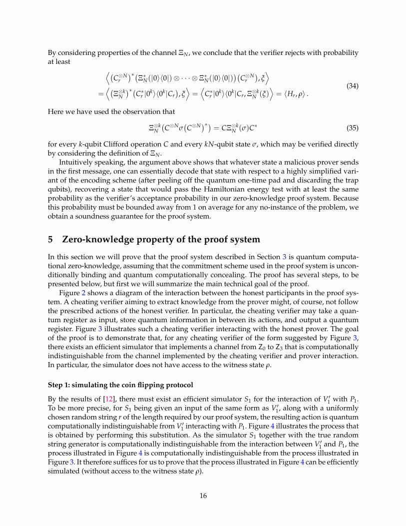
Figure 2 shows a diagram of the interaction between the honest participants in the proof sys-tem. A cheating verifier aiming to extract knowledge from the prover might, of course, not followthe prescribed actions of the honest verifier. In particular, the cheating verifier may take a quan-tum register as input, store quantum information in between its actions, and output a quantumregister. Figure 3 illustrates such a cheating verifier interacting with the honest prover. The goalof the proof is to demonstrate that, for any cheating verifier of the form suggested by Figure 3,there exists an efficient simulator that implements a channel from Z0 to Z3 that is computationallyindistinguishable from the channel implemented by the cheating verifier and prover interaction.In particular, the simulator does not have access to the witness state ρ.

Step 1: simulating the coin flipping protocol

By the results of [12], there must exist an efficient simulator S1 for the interaction of V ′1 with P1.To be more precise, for S1 being given an input of the same form as V ′1, along with a uniformlychosen random string r of the length required by our proof system, the resulting action is quantumcomputationally indistinguishable from V ′1 interacting with P1. Figure 4 illustrates the process thatis obtained by performing this substitution. As the simulator S1 together with the true randomstring generator is computationally indistinguishable from the interaction between V ′1 and P1, theprocess illustrated in Figure 4 is computationally indistinguishable from the process illustrated inFigure 3. It therefore suffices for us to prove that the process illustrated in Figure 4 can be efficientlysimulated (without access to the witness state ρ).

16

ρ P0

P1

P3

V1 V2 V3

X

(Y, z)

((t, π, a, b), s)

r

(Y, z, r)

u

(z, r, u) output

Figure 2: The interaction between honest participants. The prover’s quantum witness ρis encoded into Y together with the encoding key (t, π, a, b) by the prover’s action P0.The string z represents the prover’s commitment to (π, a, b) and the string s representsrandom bits used by the prover to implement this commitment. The string r representsthe random bits generated by the coin flipping protocol, which is depicted within thedotted rectangle on the left. The string u represents the verifier’s standard basis mea-surements for a subset of the qubits of Y determined by the challenge correspondingto the random string r. The classical zero-knowledge protocol is depicted within thedotted rectangle on the right.

ρ P0

P1

P3

V ′1 V ′2 V ′3

Z0

X

(Y, z)

((t, π, a, b), s)

r

Z1

u

Z2 Z3

Figure 3: A potentially dishonest verifier takes an auxiliary quantum register Z0 as in-put, may store quantum information (represented by registers Z1 and Z2), and outputsquantum information stored in register Z3.

Step 2: simulating the classical zero-knowledge protocol

In the next step of the proof, we replace the interaction between a cheating verifier V ′3 and theprover P3 in the classical zero-knowledge protocol by an efficient simulation.

The prover holds an encoding key (t, π, a, b) along with a random string s it has used to committo the tuple (π, a, b). The commitment z = commit((π, a, b), s) was sent to the verifier, togetherwith the encoding register Y, in the first step of the proof system. The verifier sends a string uthat, in the honest case, represents the output of a measurement of some subset of the qubitsof Y with respect to the standard basis, after the transversal application of a Clifford operationdepending on the random choice of r. The statement that the honest prover aims to prove in

17

ρ P0

coinsP3

S1 V ′2 V ′3

Z0

X

(Y, z)

((t, π, a, b), s)

r

Z1

u

Z2

r

Z3

Figure 4: The interaction corresponding to the execution of the coin flipping protocolhas been replaced by a simulator S1 along with a true random string generator (labeledcoins).

ρ P0

coinsQ

S1 V ′2 S3

Z0

X

(Y, z)

(t, π, a, b)

r

Z1

u

Z2

r

Z3

s

Figure 5: The interaction corresponding to the execution of the classical zero-knowledgeprotocol has been replaced by a simulator S3 along with the predicate Q. It is assumedthat when the output of Q is 0, the simulator S3 behaves as the cheating verifier V ′3would when the prover aborts the proof system. The string s produced by P0 in formingthe commitment to (π, a, b) is discarded.

the classical zero-knowledge protocol is that there exists an encoding key (t, π, a, b) along witha string s such that z = commit((π, a, b), s) and Q(r, t, π, a, b, u) = 1. The honest prover alwaysholds an encoding key (t, π, a, b) and a binary string s for which z = commit((π, a, b), s), and if itis the case that Q(r, t, π, a, b, u) = 0, the honest prover aborts. By the assumption that the classicalzero-knowledge protocol is indeed computational zero-knowledge, there must therefore exist anefficient simulator S3 so that the process described in Figure 5 is computationally indistinguishablefrom the one described by Figure 4. Note that the string s used by P0 to form the commitmentz = commit((π, a, b), s) can be discarded immediately after P0 is run.

Step 3: eliminating the commitment

The next step is to eliminate the commitment. Because it is assumed that the commitment schemeis quantum computationally concealing, and the commitment is never revealed by the processdescribed in Figure 5, this process is computationally indistinguishable from a similar processin which the commitment z is made to a fixed choice of a tuple (π0, a0, b0), independent of the

18

commit(π0, a0, b0)

S1 V ′2

V ′

Z0

z

Z1

Y u

r

Z2

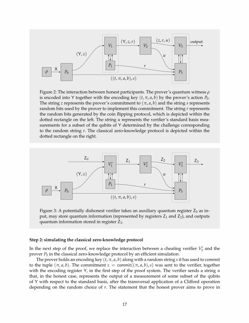
Figure 6: The commitment to a fixed tuple (π0, a0, b0), the simulator S1, and the dishon-est verifier action V ′2 may be merged into a single efficiently implementable action V ′

that represents an attack against the encoding scheme.

E

V ′

Qcoins

ρ

r

r

Y

Z0

(t, π, a, b)

u

Z2

X

Figure 7: A cheating verifier V ′ aims to extract knowledge from the encoding of a reg-ister X.

prover’s encoding key. In particular, one may take π0 to be the identity permutation and a0 andb0 to be all-zero strings of length 2nN. One may now consider the commitment to this fixed tuple(π0, a0, b0), together with the simulator S1 and the cheating verifier action V ′2, to form a single,efficiently implementable action V ′ as suggested by Figure 6.

The interaction between this new action V ′ and the prover’s encoding, the random string gen-erator, and the predicate Q, as is illustrated in Figure 7, may now be considered. If it is proved thatthe channel implemented by this process can be efficiently simulated, then it will follow that thechannel implemented by the process described in Figure 5 can be efficiently simulated (in a com-putationally indistinguishable sense). This is so because the composition of the process illustratedin Figure 7 with the efficiently implementable simulator S3 is computationally indistinguishablefrom the process described in Figure 5.

Step 4: simulating an attack on the encoding scheme

It therefore suffices for us to prove that, for any efficiently implementable action V ′, the channelimplemented by the process described by Figure 7 can be efficiently simulated. In fact, it will bepossible to efficiently simulate this channel with statistical accuracy, not just in a computation-ally indistinguishable sense. This is not surprising: we have claimed that the computational zero-

19

E

V ′

Q

coins

ρr

r

r

Y

Z0

(t, π, a, b)

u

Z2

r

Figure 8: The simulation of the process shown in Figure 7 is nearly identical to thatprocess, except that it uses the random string r to encode a state ρr that is guaranteedto pass the challenge corresponding to r, rather than encoding the witness state ρ.

E

V ′r

Qrξ

Y

Z0

(t, π, a, b)

u

Z2

Figure 9: An arbitrary n-qubit state ξ is encoded, and the cheating verifier V ′ and pred-icate Q for a fixed choice of a string r interact as depicted. It will be proved that thechannels obtained by substituting ρ and ρr for ξ are approximately equal.

knowledge property of our proof system is based on a computationally concealing commitmentscheme, and the uses of the commitment scheme have all been eliminated from consideration bythe steps above.

At this point we may describe the simulator directly: it is illustrated in Figure 8, and it repre-sents the most straightforward approach to obtaining a simulator. This simulator differs from theprocess described in Figure 7 in that it uses the output of the random string generator to choosea quantum state that, once encoded, passes the randomly selected challenge with certainty. It istrivial to efficiently prepare such a state given the string r. It remains to prove that the channelimplemented by the simulator described in Figure 8 is indistinguishable from the channel imple-mented by the process described in Figure 7. By convexity it suffices to prove that this is so forevery fixed choice of the string r.

With this goal in mind, consider the process described in Figure 9, in which an arbitrary state ξis encoded (corresponding either to ρ or ρr in Figures 7 and 8), and the string r is fixed (which hasbeen indicated by the substitution of V ′r and Qr for V ′ and Q, respectively). We will prove that thechannel implemented by any such process can have only a limited dependence on the state ξ.

More specifically, let us assume that ξ0 and ξ1 are arbitrary n-qubit states, let p0 and p1 denotethe probabilities with which these two states would pass the challenge determined by r (for anhonest prover and verifier pair), and let Ψ0 and Ψ1 denote the channels from Z0 to Z2 together

20

V ′rXcZdCr C∗r Xc wY

Z0 Z2

Z0

Y

V ′′r

Cr

Z2

wv

Figure 10: The prover’s one-time pad merged with the cheating verifier operation V ′r .Averaging over random choices of c and d results in a process that can alternatively bedescribed as illustrated in the lower diagram. In this process, V ′′r represents a so-calledquantum instrument, which transforms Z0 into Z2 and produces a classical measurementoutcome. In this case, this classical measurement outcome is XORed onto the stringproduced by a standard basis measurement. (In this figure and the next, one should in-terpret Cr and C∗r as referring to the transversal application of the corresponding Cliffordoperation.)

with the output bit of the predicate Qr that are implemented by the process shown in Figure 9when ξ0 or ξ1 is substituted for ξ, respectively.

We claim that if the difference |p0 − p1| is negligible, then the distance ‖Ψ0 −Ψ1‖ is also negli-gible. The two steps that follow establish that this claim is true. By the assumption that the proverinitially holds a witness state ρ that satisfies every Hamiltonian term with probability exponen-tially close to 1, this will complete the proof.

Step 5: twirling the cheating verifier

To prove the fact suggested above regarding the channel implemented by Figure 9, we will natu-rally need to make use of the specific properties of the encoding scheme, which has not played animportant role in the analysis thus far. The first step is to recognize that the effect of the prover’sone time pad is to twirl3 the verifier as Figure 10 illustrates.

In greater detail, the last step of the encoding process is the quantum one-time pad: the proverindependently chooses one of the Pauli operations 1, X, Z, or XZ for each qubit of Y and appliesthat operation, storing the randomly selected strings a, b ∈ Σ2Nn. With respect to the Cliffordoperation Cr associated with the randomly selected challenge (determined by the string r), theprover computes the pair (c, d) for which it holds that

XaZb =(C⊗2N

r)∗XcZd(C⊗2N

r). (36)

The first step when computing the predicate Qr is the application of Xc to the string u, which issupposed to represent the outcome of a standard basis measurement of a subset of the qubits afterthe transversal application of Cr to the corresponding qubits in the register Y. The resulting string

3The term twirl is commonly used in quantum information theory to describe a process whereby a symmetrizationover a collection of randomly chosen unitary operations has a particular effect on a state or channel. Twirled states andchannels often take on a significantly simpler form than the original state or channel prior to twirling.

21

F Rrξ

CrY

(t, π)

w

v

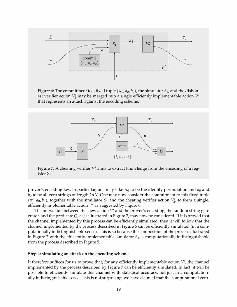
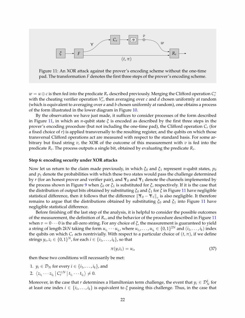
Figure 11: An XOR attack against the prover’s encoding scheme without the one-timepad. The transformation F denotes the first three steps of the prover’s encoding scheme.

w = u⊕ c is then fed into the predicate Rr described previously. Merging the Clifford operation C∗rwith the cheating verifier operation V ′r , then averaging over c and d chosen uniformly at random(which is equivalent to averaging over a and b chosen uniformly at random), one obtains a processof the form illustrated in the lower diagram in Figure 10.

By the observation we have just made, it suffices to consider processes of the form describedin Figure 11, in which an n-qubit state ξ is encoded as described by the first three steps in theprover’s encoding procedure (but not including the one-time pad), the Clifford operation Cr (fora fixed choice of r) is applied transversally to the resulting register, and the qubits on which thosetransversal Clifford operations act are measured with respect to the standard basis. For some ar-bitrary but fixed string v, the XOR of the outcome of this measurement with v is fed into thepredicate Rr. The process outputs a single bit, obtained by evaluating the predicate Rr.

Step 6: encoding security under XOR attacks

Now let us return to the claim made previously, in which ξ0 and ξ1 represent n-qubit states, p0and p1 denote the probabilities with which these two states would pass the challenge determinedby r (for an honest prover and verifier pair), and Ψ0 and Ψ1 denote the channels implemented bythe process shown in Figure 9 when ξ0 or ξ1 is substituted for ξ, respectively. If it is the case thatthe distribution of output bits obtained by substituting ξ0 and ξ1 for ξ in Figure 11 have negligiblestatistical difference, then it follows that the difference ‖Ψ0 −Ψ1‖ is also negligible. It thereforeremains to argue that the distributions obtained by substituting ξ0 and ξ1 into Figure 11 havenegligible statistical difference.

Before finishing off the last step of the analysis, it is helpful to consider the possible outcomesof the measurement, the definition of Rr, and the behavior of the procedure described in Figure 11when v = 0 · · · 0 is the all-zero string. For any choice of ξ, the measurement is guaranteed to yielda string of length 2kN taking the form ui1 · · · uik , where ui1 , . . . , uik ∈ 0, 12N and (i1, . . . , ik) indexthe qubits on which Cr acts nontrivially. With respect to a particular choice of (t, π), if we definestrings yi, zi ∈ 0, 1N , for each i ∈ i1, . . . , ik, so that

π(yizi) = ui, (37)

then these two conditions will necessarily be met:

1. yi ∈ DN for every i ∈ i1, . . . , ik, and

2.⟨zi1 · · · zik

∣∣C⊗Nr∣∣ ti1 · · · tik

⟩6= 0.

Moreover, in the case that r determines a Hamiltonian term challenge, the event that yi ∈ D1N for

at least one index i ∈ i1, . . . , ik is equivalent to ξ passing this challenge. Thus, in the case that

22

v = 0 · · · 0, the process described in Figure 11 outputs the bit 1 with precisely the probability thatan honest prover and verifier pair would result in acceptance, assuming the prover’s initial stateis ξ and r is selected as a random string determining the challenge.

Now let us assume that v is a nonzero string, and let us consider two cases: the first is thatthe Hamming weight |v|1 of v satisfies |v|1 < K, for K being the minimum Hamming weight of anonzero codeword in DN , and the second case is that |v|1 ≥ K.

If it is the case that |v|1 < K, then there are two possible ways that the value of the predicate Rrcould change, in comparison to the case v = 0 · · · 0. In both cases, if there is a change, it must befrom 1 to 0, caused by one of the two conditions above becoming violated. The first case is that oneor more bits in one of the codewords yi1 , . . . , yik is flipped, causing the first condition listed aboveto become violated. The second case is that a measurement outcome for the trap qubits is obtainedthat potentially violates the second condition. Note that it is not possible that the first conditionremains satisfied, but the Hamiltonian term challenge condition that yi ∈ D1

N for at least one indexi ∈ i1, . . . , ik changes, as such a change would require at least K bit-flips to cause a logical changein valid codewords. It is unimportant for the purposes of the analysis to determine the probabilitywith which one of the two conditions becomes violated, except to observe that it is independentof ξ. (In somewhat more detail, the string v may be written as v = vi1 · · · vik , and the probabilitythat neither of the two conditions is affected is given by the probability that π−1(vi) places no 1swithin the first N bits or over a trap qubit left in a standard basis state within the second N bits,for a random choice of π and for each i ∈ i1, . . . , ik.)

If it is the case that |v|1 ≥ K, then there is a possibility that, in comparison to the functioning ofthe process for v = 0 · · · 0, the Hamiltonian term challenge condition that yi ∈ D1

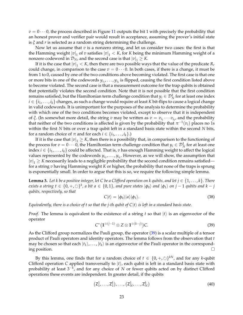
N for at least oneindex i ∈ i1, . . . , ik could be affected. That is, v has enough Hamming weight to affect the logicalvalues represented by the codewords yi1 , . . . , yik . However, as we will show, the assumption that|v|1 ≥ K necessarily leads to a negligible probability that the second condition remains satisfied—for a string v having Hamming weight K or higher, the probability that none of the traps is sprungis exponentially small. In order to argue that this is so, we require the following simple lemma.

Lemma 3. Let k be a positive integer, let C be a Clifford operation on k qubits, and let j ∈ 1, . . . , k. Thereexists a string t ∈ 0,+,k, a bit a ∈ 0, 1, and pure states |φ0〉 and |φ1〉 on j− 1 qubits and k − jqubits, respectively, so that

C|t〉 = |φ0〉|a〉|φ1〉. (38)

Equivalently, there is a choice of t so that the j-th qubit of C|t〉 is left in a standard basis state.

Proof. The lemma is equivalent to the existence of a string t so that |t〉 is an eigenvector of theoperator

C∗(1⊗(j−1) ⊗ Z⊗ 1⊗(k−j))C. (39)

As the Clifford group normalizes the Pauli group, the operator (39) is a scalar multiple of a tensorproduct of Pauli operators and identity operators. The lemma follows from the observation that tmay be chosen so that each |t1〉, . . . , |tk〉 is an eigenvector of the Pauli operator in the correspond-ing position.

By this lemma, one finds that for a random choice of t ∈ 0,+,kN , and for any k-qubitClifford operation C applied transversally to |t〉, each qubit is left in a standard basis state withprobability at least 3−k, and for any choice of N or fewer qubits acted on by distinct Cliffordoperations these events are independent. In greater detail, if the qubits(

Z11, . . . ,Zk

1), . . . ,

(Z1

N , . . . ,ZkN)

(40)

23

are initialized to the state |t〉, for t ∈ 0,+,kN chosen uniformly at random, and the k-qubitClifford operation C is applied independently to each k-tuple of qubits, then each qubit is leftin a standard basis state with probability at least 3−k, and the states of the k-tuples of qubits areindependent.

Now we return to the analysis for a string v of length 2kN having Hamming weight at least K.By virtue of the fact just mentioned, it is straightforward to obtain a negligible upper-bound onthe probability for the process described in Figure 11 to output 1. As this event requires that arandom choice of the permutation π leaves none of the 1-bits of v in positions corresponding totrap qubits left in standard basis states by the transversal action of Cr, we find that the probabilityto output 1 is exponentially small in K. In particular, this probability is at most(

1− 13k+1

)K/k

= exp(−ε(k)K) (41)

where ε(k) denotes a positive real number depending on k but not K.From a consideration of the two cases just presented, we may conclude the following. Suppose

as before that ξ0 and ξ1 are n-qubit states that may be substituted for ξ in Figure 11, and that theprobabilities p0 and p1 for these states to pass the challenge determined by a fixed choice of rhave negligible difference. Let us write q0(v) and q1(v), respectively, to denote the probability thatthe process described in Figure 11 outputs 1. As noted before, it holds that p0 = q0(0 · · · 0) andp1 = q1(0 · · · 0). For any choice of v satisfying |v|1 < K, we have that q0(v) = β(v)q0(0 · · · 0) andq1(v) = β(v)q1(0 · · · 0) for β(v) ∈ (0, 1) that is independent of ξ0 and ξ1. Finally, for any choiceof v satisfying |v|1 ≥ K, we have that q0(v) and q1(v) are both negligible. It therefore follows thatthe difference |q0(v)− q1(v)| is negligible in all cases, which completes the proof.

6 Conclusion

This paper gives a zero-knowledge proof system for any problem in QMA assuming the existenceof a quantum computationally concealing and unconditionally binding commitment scheme. Sucha commitment scheme can be obtained assuming quantum-secure one-way permutations [1] (orinjections more generally) or a quantum-secure pseudo-random generator [40] that could poten-tially be based on one-way functions that are hard to invert for any quantum polynomial timealgorithm [29, 43, 52]. We conclude with a few open questions and directions for future work.

1. Our proof system inherits the soundness error of the most straightforward verification proce-dure for the local Clifford-Hamiltonian problem, which is to randomly select a Hamiltonianterm and perform a measurement corresponding to it. When an arbitrary QMA problem isreduced to the local Hamiltonian problem, the resulting soundness error may potentially belarge (polynomially bounded away from 1). Can one obtain a zero-knowledge proof systemfor any QMA problem with small soundness error while maintaining the other features of ourproof system (e.g., constant round of communications)?

We note that if a prover has polynomially many copies of a valid quantum witness, then aparallel repetition of our proof system may yield a constant round zero-knowledge proof sys-tem having small soundness error for any QMA problem—but this would require a paral-lel repetition result concerning zero-knowledge proof systems for NP secure against quan-tum attacks. Analogous results for zero-knowledge proofs for NP against classical attacks areknown [15, 19], but they involve sophisticated rewinding arguments for which known quan-tum rewinding techniques do not seem to be applicable.

24

2. Are there natural formalizations of proofs of quantum knowledge? Roughly speaking, one wouldexpect such a notion to require that whenever a prover is able to prove the validity of a state-ment, one could construct a knowledge extractor that can extract a quantum witness givenaccess to such a prover. It seems plausible that our proof system could be adapted to such anotion, although we have not investigated this notion in depth.

3. We have considered an encoding scheme for quantum states that ensures the secrecy of thestate and allows for the transversal application of constant-size Clifford operations and mea-surement in the computational basis. It is an interesting open question to extend our encodingscheme, or to design a new one, so that it can support transversally applying a larger family ofquantum operations.

4. Finally, we make one further remark on an abstract view of our proof system. Classically speak-ing, one can imagine a “commit-and-open” primitive where a sender commits to a message m,and later opens sufficient information so that a receiver can test a property P(·) on m, andnothing more. For example, P can be an NP-relation R(x, ·) that checks if message m is a validwitness. This can be implemented easily by a standard commitment scheme and during theopening phase, the sender and receiver run a zero-knowledge proof of R(x, m) = 1 instead ofthe standard opening. Our proof system, which combines a commitment scheme and classicalzero-knowledge proofs for NP, can be viewed as a quantum analogue. Namely, we commit toa witness state and open just enough information to verify that some reduced density of thewitness state falls into a specific subspace. We can only deal with properties of a very specialform, and it is an interesting direction for future work to generalize and find applications ofthis sort of primitive.

Acknowledgments

We thank Michael Beverland, Sevag Gharibian, David Gosset, Yi-Kai Liu and Bei Zeng for helpfulconversations. A. B. and J. W. are supported in part by Canada’s NSERC. F. S. is supported in partby Cryptoworks21, Canada’s NSERC and CIFAR.

25

A Preliminaries

This section summarizes some of the notation, definitions, and known facts concerning quantuminformation and computation, cryptography, and other topics that are used throughout the paper.We refer to [34, 41, 48] for further details on the theory of quantum information and computation.Further information on classical zero-knowledge and cryptography can be found in [17, 18].

A.1 Basic terminology

Throughout the paper we let Σ = 0, 1 denote the binary alphabet, and only consider strings,promise problems, and complexity classes over this alphabet. For a string x ∈ Σ∗, |x| denotesits length. A function g : N → N is a polynomially bounded function if there exists a determin-istic polynomial-time Turing machine Mg that outputs 1g(n) on input 1n for every non-negativeinteger n. A function f : N → [0, ∞) is said to be negligible if, for every polynomially boundedfunction g, it holds that f (n) < 1/g(n) for all but finitely many values of n.

A.2 Quantum information basics

When we refer to a quantum register in this paper, we simply mean a collection of qubits that wewish to view as a single unit and to which we give some name. Names of registers will always beuppercase letters in a sans serif font, such as X, Y, and Z. The finite dimensional complex Hilbertspaces associated with registers will be denoted by capital script letters such as X , Y , andZ , usingthe same letter in the two different fonts to denote a quantum register and its corresponding spacefor convenience. Dirac notation is used to express vectors in Hilbert spaces and linear mappingsbetween them in a standard way.

For a given space X , we let L(X ) denote the set of all linear mappings (or operators) from X toitself. The identity element of L(X ) is denoted 1X , or just as 1 when X can be taken as implicit.The inner product between operators A and B is defined as 〈A, B〉 = Tr(A∗B).

Quantum states are represented by density operators, which are positive semidefinite operatorshaving unit trace. A linear map Φ : L(X ) → L(Y) is said to be a channel if it is both completelypositive and trace-preserving. Channels are mappings from density operators to density opera-tors that, in principle, represent physically realizable operations. A measurement is described by acollections of positive semidefinite operators Mj such that ∑j Mj = 1, with the probability thatthe measurement on state ρ results in outcome j being given by

⟨Mj, ρ

⟩We review a few definitions of norms on operators, which are used to discuss the distin-

guishability of quantum states and channels. The trace norm of an operator X ∈ L(X ) is definedas ‖X‖1 = Tr

√X∗X. For any linear map Φ : L(X ) → L(Y), the diamond norm (or completely

bounded trace norm) [3, 33, 34] is defined as

‖Φ‖ = max∥∥∥(Φ⊗ 1L(W))(X)

∥∥∥1

: X ∈ L(X ⊗W) , ‖X‖1 ≤ 1

,

where W is any space with dimension equal to that of X . (The value remains the same for anychoice ofW , provided its dimension is at least that of X .)

Quantum gates and circuits

A quantum circuit is an acyclic network of quantum gates connected by wires. The quantum gatesrepresent quantum channels while the wires represent qubits on which the channels act.

26

We will refer to two types of quantum circuits in this paper: unitary quantum circuits and gen-eral quantum circuits. By unitary quantum circuits we mean circuits composed of unitary gates(such as the ones described below) chosen from some finite gate set. General quantum circuitsare composed of gates that may correspond to channels that are not necessarily unitary. It is suf-ficient for the purposes of this paper that we consider just two simple non-unitary gates: ancillarygates, which input nothing and output a qubit in the |0〉 state; and erasure gates, which input onequbit and output nothing (and correspond to the channel described by the trace mapping). Asis described elsewhere [3, 50], arbitrary channels mapping one register to another can always beapproximated arbitrarily closely by quantum circuits whose gates include a universal collection ofunitary gates together with ancillary and erasure gates. The size of a quantum circuit is the numberof gates in the circuit plus the number of qubits on which it acts.

We will refer to the following well-known single-qubit unitary gates:

1. Pauli gates:X : |a〉 7→ |1− a〉 and Z : |a〉 7→ (−1)a|a〉, (42)

for each a ∈ 0, 1, as well as Y = iXZ.

2. Hadamard gate:

H : |a〉 7→ 1√2|0〉+ (−1)a

√2|1〉, (43)

for each a ∈ 0, 1.3. Phase gate:

P : |a〉 7→ ia|a〉, (44)

for each a ∈ 0, 1.

In addition, for any k-qubit unitary quantum gate U we define the controlled-U gate as

Λ(U) : |a〉|x〉 7→ |a〉Ua|x〉, (45)

for each a ∈ 0, 1 and x ∈ 0, 1k.The k-qubit Pauli group is the group containing all unitary operators of the form

αU1 ⊗ · · · ⊗Uk (46)

where α ∈ 1, i,−1,−i and U1, . . . , Uk ∈ 1, X, Y, Z, where 1 denotes the single-qubit identityoperation. Elements of this group are also referred to as Pauli operations. If a, b ∈ 0, 1k are binarystrings of length k, then we write

Xa = Xa1 ⊗ · · · ⊗ Xak and Zb = Zb1 ⊗ · · · ⊗ Zbk (47)

to denote the Pauli operations obtained from these strings as indicated.Channels that can be expressed as convex combinations of unitary channels that correspond

to Pauli operations are called Pauli channels. An example of Pauli channels that is relevant to thispaper is the completely depolarizing channel

Ω(ρ) =14 ∑

a,b∈0,1

(XaZb)ρ(XaZb)∗ = 1

2, (48)

for any single-qubit density operator ρ. We thus see that the effect of Ω is to completely randomizethe state of a single-qubit system. By treating a random choice of a pair (a, b) as a secret key, we

27

obtain a quantum generalization of the one-time pad, known as the quantum one-time pad [4]. Whenthe channel is performed independently on k qubits, the effect is given by

Ω⊗k(ρ) = 2−k 1⊗ · · · ⊗ 1 (49)

for every k-qubit density operator ρ. The quantum one-time pad generalizes naturally to anychoice of the number k.

Sometimes it will be convenient to consider quantum circuits that implement measurements.When we refer to a measurement circuit, we mean any general quantum circuit, followed by a mea-surement of all of its output qubits with respect to the standard basis. If Q is a measurement circuitthat is applied to a collection of qubits in the state ρ, then Q(ρ) is interpreted as a string-valuedrandom variable describing the resulting measurement. We will only need to refer to measurementcircuits outputting a single bit in this paper.

A k-qubit Clifford circuit is any unitary quantum circuit on k qubits whose gates are drawnfrom the set H, P, Λ(X) containing Hadamard, phase, and controlled-not gates. (It is commonthat one also allows Pauli gates to be included in this set for convenience. Given that X = HPPHand Z = PP, there is no generality lost in using the smaller gate set in the definition.) The set of allunitary operators that can be described by k-qubit Clifford circuits forms a finite group known asthe Clifford group. Up to scalar multiples, the k-qubit Clifford group is the normalizer of the k-qubitPauli group: if U is a k-qubit unitary operator for which it holds that UVU∗ is an element of thek-qubit Pauli group for every k-qubit Pauli group element V, then U = αC for α ∈ C satisfying|α| = 1 and C being a k-qubit Clifford group element. Given the description of a k-qubit Pauligroup element V and a k-qubit Clifford circuit C, one can efficiently compute a description of thek-qubit Pauli group element CVC∗ [26].

Clifford circuits are not universal for quantum computation. Two examples (among otherknown examples) of universal gate sets are the following:

1. Hadamard, phase, and Toffoli gates: H, P, Λ(Λ(X)).2. Hadamard and controlled-phase gates: H, Λ(P).

The first of these choices is sometimes easier to work with, but we will make use of the fact thatthe second gate set is universal in the paper.

A.3 Polynomial-time generated families of quantum circuits and QMA

Any quantum circuit with gates drawn from a fixed, finite gate set can be encoded as a binarystring, with respect to a variety of possible encoding schemes. The specific details of such encodingschemes are not important within the context of this paper, so we will leave it to the reader toimagine that a sensible and efficient encoding scheme for quantum circuits has been selected,relative to whatever gate set is under consideration. It should be assumed, of course, that a circuit’ssize and its encoding length are polynomially related.

For any infinite set of binary strings S ⊆ 0, 1∗, a collection Vx : x ∈ S of quantum cir-cuits is said to be polynomial-time generated if there exists a deterministic polynomial-time Turingmachine that, on input x ∈ S, outputs an encoding of Vx. The assumptions on encoding schemessuggested above imply that, if Vx : x ∈ S is a polynomial-time generated collection, then Vxmust have size polynomial in |x|.

Next we will define the complexity class QMA, which is commonly viewed as the most naturalquantum generalization of NP.

28

Definition 4. A promise problem A = (Ayes, Ano) is contained in the complexity class QMAα,β ifthere exists a polynomial-time generated collection

Vx : x ∈ Ayes ∪ Ano

(50)

of quantum circuits and a polynomially bounded function p possessing the following properties:

1. For every string x ∈ Ayes ∪ Ano, one has that Vx is a measurement circuit taking p(|x|) inputqubits and outputting a single bit.

2. Completeness. For all x ∈ Ayes, there exists a p(|x|)-qubit state ρ such that Pr(Vx(ρ) = 1) ≥ α.

3. Soundness. For all x ∈ Ano, and every p(|x|)-qubit state ρ, it holds that Pr(Vx(ρ) = 1) ≤ β.

In this definition, α, β ∈ [0, 1] may be constant values or functions of the length of the inputstring x. When they are omitted, it is to be assumed that they are α = 2/3 and β = 1/3. Knownerror reduction methods [34, 37] imply that a wide range of selections of α and β give rise tothe same complexity class. In particular, QMA coincides with QMAα,β for α = 1 − 2−q(|x|) andβ = 2−q(|x|), for any polynomially bounded function q.

A.4 Quantum computational indistinguishability and zero-knowledge

Next we review notions of quantum state and channel discrimination, as well as zero-knowledgein a quantum setting (as defined in [49]).

We first specify what it means for two collections of quantum states to be quantum compu-tationally indistinguishable. The definition that follows may be viewed as being a non-uniformnotion of quantum computational indistinguishability, as it places no uniformity conditions onquantum circuits and allows for an auxiliary quantum state σ to assist in the task of state discrimi-nation.

Definition 5 (Quantum computationally indistinguishable states). Suppose that S ⊆ 0, 1∗ isan infinite set of binary strings, r is a polynomially bounded function, and ρx and ξx are stateson r(|x|) qubits for each x ∈ S. The collections ρx : x ∈ S and ξx : x ∈ S are quantumcomputationally indistinguishable if, for every choice of polynomially bounded functions s and k,any measurement circuit Q of size s(|x|), and any choice of a k(|x|)-qubit state σ, it holds that

|Pr[Q(ρx ⊗ σ) = 1]− Pr[Q(ξx ⊗ σ) = 1]| ≤ ε(|x|) (51)

for all x ∈ S, for a negligible function ε.

The notion extends naturally to distinguishing collections of channels, as the following defini-tion makes precise.

Definition 6 (Quantum computationally indistinguishable channels). Suppose that S ⊆ 0, 1∗is an infinite set of binary strings, q and r are polynomially bounded functions, and Φx and Ψxare channels from q(|x|) qubits to r(|x|) qubits for each x ∈ S. The collections Φx : x ∈ S andΨx : x ∈ S are quantum computationally indistinguishable if, for every choice of polynomiallybounded functions s and k, every state σ on q(|x|) + k(|x|) qubits, and every measurement circuitQ on r(|x|) + k(|x|) qubits having size s(|x|), one has that

|Pr[Q((Φx ⊗ 1)(σ)) = 1]− Pr[Q((Ψx ⊗ 1)(σ)) = 1]| ≤ ε(|x|) (52)

for every x ∈ S, for a negligible function ε.

29

We will also make use of statistical notions of indistinguishability for states and channels,which are defined as follows.

Definition 7 (Statistically indistinguishable states). Suppose that S ⊆ 0, 1∗ is an infinite set ofbinary strings, r is a polynomially bounded function, and ρx and ξx are states on r(|x|) qubits foreach x ∈ S. The collections ρx : x ∈ S and ξx : x ∈ S are statistically indistinguishable if

12‖ρx − ξx‖1 ≤ ε(|x|) (53)

for all x ∈ S, for a negligible function ε.

Definition 8 (Statistically indistinguishable channels). Suppose that S ⊆ 0, 1∗ is an infinite setof binary strings, q and r are polynomially bounded functions, and Φx and Ψx are channels fromq(|x|) qubits to r(|x|) qubits for each x ∈ S. The collections Φx : x ∈ S and Ψx : x ∈ S arestatistically indistinguishable if

12‖Φx −Ψx‖ ≤ ε(|x|) (54)

for all x ∈ S, for a negligible function ε.

Next we review the definition of quantum computational zero-knowledge proof systems asdefined in [49]. Let (P, V) be a quantum or classical interactive proof system for a promise prob-lem A. An arbitrary (possibly malicious) verifier V ′ is any quantum computational process thatinteracts with P according to the structural specification of (P, V). Similar to the classical notionof auxiliary input zero-knowledge, a verifier V ′ will take, in addition to the input string x, anauxiliary input, and produce some output. This is crucial for the composition of zero-knowledgeproof systems. The most general situation allowed by quantum information theory is that boththe auxiliary input and the output are quantum, meaning that the verifier operates on quantumregisters whose initial state is arbitrary and may be entangled with some external system. Alsosimilar to the classical case, we will assume that for any given polynomial-time verifier V ′ thereexist polynomially bounded functions q and r that determine the number of auxiliary input qubitsand output qubits of V ′. To say that V ′ is a polynomial-time verifier means that the entire actionof V ′ must be described by some polynomial-time generated family of quantum circuits.

The interaction of a verifier V ′ with P on input x induces some channel from the verifier’sq(|x|) auxiliary input qubits to r(|x|) output qubits. LetW denote the vector space correspondingto the auxiliary input qubits, let Z denote the space corresponding to the output qubits, and letΦx : L(W) → L(Z) denote the resulting channel induced by the interaction of V ′ with P oninput x. A simulator S for a given verifier V ′ is described by a polynomial-time generated familyof general quantum circuits that agrees with V ′ on the functions q and r representing the numberof auxiliary input qubits and output qubits respectively. Such a simulator does not interact with P,but simply induces a channel that we will denote by Ψx : L(W)→ L(Z) on each input x.

Definition 9 (Quantum computational zero-knowledge). An interactive proof system (P, V) fora promise problem A is quantum computational zero-knowledge if, for every polynomial-time gen-erated quantum verifier V ′, there exists a polynomial-time generated quantum simulator S thatsatisfies the following requirements.

1. The verifier V ′ and simulator S agree on the polynomially bounded functions q and r thatspecify the number of auxiliary input qubits and output qubits, respectively.

2. Let Φx be the channel that results from the interaction between V ′ and P on input x, and let Ψxbe the channel induced by the simulator S on input x, both as described above. Then the col-lections Φx : x ∈ Ayes and Ψx : x ∈ Ayes are quantum computationally indistinguishable.

30

A.5 Cryptographic Tools

Here we introduce a few cryptographic building blocks that are useful in our proof system. Weemphasize that, as is typical in the classical setting, we formulate all computational security prop-erties (e.g., concealing in a commitment scheme) with respect to non-uniform quantum adver-saries. This is inherited from the definition of quantum computational indistinguishability. Thisgives more stringent security requirements and is also crucial in security proofs.

Commitment schemes

For the sake of simplicity, we describe a commitment scheme that is non-interactive, i.e., all mes-sages are going from a sender to a receiver. A similar definition can be derived for interactiveschemes.

Definition 10 (Quantum computationally secure commitment schemes). A quantum computation-ally secure commitment scheme for an alphabet Γ is a collection of polynomial-time computable func-tions fn : n ∈N taking the form

fn : Γ× 0, 1p(n) → 0, 1q(n), (55)

for polynomially bounded functions p and q, such that the following conditions hold:

1. Unconditionally binding property. For every choice of n ∈ N, a, b ∈ Γ, and r, s ∈ 0, 1p(n), onehas that fn(a, r) = fn(b, s) implies a = b.

2. Quantum computationally concealing property. For every a ∈ Γ and n ∈N, define

ρa,n =1

2p(n) ∑r∈0,1p(n)

| fn(a, r)〉〈 fn(a, r)|. (56)

For every choice of a, b ∈ Γ the ensembles ρa,n : n ∈ N and ρb,n : n ∈ N are quantumcomputationally indistinguishable.

To commit to a string, one can independently use the commitment described above bit bybit. Such a commitment scheme can be constructed based on certain quantum intractability as-sumptions. As shown in [1], it suffices to have quantum-resistant one-way permutations, which arepermutations that can be computed efficiently on a classical computer but are hard to invert forboth classical and quantum polynomial-time algorithms. The same commitment scheme remainsquantum-secure based on a slightly weaker assumption of quantum-resistant injective one-wayfunctions. Naor showed a commitment scheme with a two-message commit phase [40] which willbe quantum-secure [28], assuming one uses a pseudo-random generator whose output is quantumcomputationally indistinguishable from a truly random string4.

Based on such a quantum-secure commitment scheme, we can obtain the other two essentialcryptographic building blocks in our protocol: a zero-knowledge proof system for NP and a coin-flipping protocol, both secure against quantum adversaries.

4It has been stated informally (see e.g., [43,52]) that the pseudo-random generator by Hastad et al. [29] based on one-way functions would remain quantum-secure, so long as the one-way functions are resistant to any polynomial-timequantum inverting algorithms.

31

Zero-knowledge proof for NP

Watrous showed that [49] the GMW 3-Coloring protocol [21] remains zero-knowledge in the pres-ence of quantum verifiers, assuming a statistically binding and quantum computationally hidingcommitment scheme. This means that we have a classical zero-knowledge proof protocol for anyNP language that is secure against any polynomial-time quantum verifiers.

Coin-flipping

A coin-flipping protocol is an interactive process that allows two parties to jointly toss randomcoins. It is not necessary for us to consider this notion generally, as we only make use of onespecific coin-flipping protocol, namely Blum’s coin-flipping protocol [8] in which an honest provercommits to a random y ∈ 0, 1, the honest verifier selects z ∈ 0, 1 at random, the proverreveals y, and the two participants agree that the random bit generated r = y⊕ z.

Damgard and Lunemann [12] proved that Blum’s coin-flipping protocol is quantum-secure,assuming a quantum-secure commitment scheme. This protocol generates one random coin, andwe will need to flip logarithmic many random bits. A simple way of achieving this is by sequentialrepetition, but more effectively it is possible to extend the analysis of Damgard and Lunemann andshow that parallel repetition of Blum’s protocol logarithmic many times remains quantum-secure.

A.6 Concatenated Steane codes

The last topic to be discussed in this section concerns the existence of quantum error correctingcodes having certain properties that are important to the functioning of our zero-knowledge proofsystem for QMA. There are multiple choices of codes that satisfy our requirements, but in theinterest of simplicity we will describe just one specific family of codes in this category.

These codes are based on the 7-qubit Steane code [44], in which one qubit is encoded into 7qubits by the following action on standard basis states:

|0〉 7→ 1√8

∑x∈D0

7

|x〉 and |1〉 7→ 1√8

∑x∈D1

7

|x〉, (57)

where

D07 = 0000000, 0001111, 0110011, 0111100, 1010101, 1011010, 1100110, 1101001,D1

7 = 0010110, 0011001, 0100101, 0101010, 1000011, 1001100, 1110000, 1111111.(58)

It is the case that D07 is a [7, 4]-Hamming code, while

D7 = D07 ∪D1

7 (59)

is the dual code to D07 (i.e., it is the code consisting of all binary strings of length 7 whose inner

product with any codeword inD07 is even). This is an example of a CSS code [41], and it is capable of

correcting single-qubit errors. The standard error-correcting procedure, which we do not actuallyneed in this paper, is to first reversibly correct errors in the standard basis, with respect to thecode D7, and then to do the same with respect to the diagonal basis. The 7-qubit Clifford circuitdepicted in Figure 12 encodes one qubit into 7 with respect to this code, assuming 6 qubits inthe |0〉 state are made available.

32

|ψ〉

|0〉

|0〉

|0〉

|0〉

|0〉

|0〉

H

H

H

Figure 12: A Clifford circuit encoder for the 7-qubit Steane code. Hereafter we will writeU7 to refer to the unitary operator on 7 qubits described by this circuit.

One of the properties of the 7-qubit Steane code that is important from the viewpoint of thispaper is that it admits a transversal application of Clifford operations, in the sense that is explainedin Figure 13.

Note that by concatenating the 7-qubit Steane code with itself, one obtains a code having simi-lar properties to the 7-qubit code, and in addition having a large minimum distance for the under-lying code. More specifically, suppose that N = 7t for t being an even positive integer. (We taket to be even for convenience, as this eliminates the entry-wise complex conjugation on Cliffordoperations encountered in the discussion of their transversal application.) By concatenating the7-qubit Steane code to itself t times, one obtains a quantum error-correcting code in which onequbit is encoded into N qubits in the following way:

|0〉 7→ 1√8t ∑

x∈D0N

|x〉 and |1〉 7→ 1√8t ∑

x∈D1N

|x〉 (60)

where D0N ,D1

N ⊆ 0, 1N are related in a way that generalizes the case N = 7. In particular, D0N is

a binary linear code having 8t elements, and whose dual code takes the form

DN = D0N ∪D1

N (61)

for D1N ⊆ 0, 1N being a coset of D0

N .As a quantum error correcting code, the t-fold concatenation of the 7-qubit Steane code inherits

the properties of the 7-qubit Steane code mentioned above. A Clifford circuit UN acting on Nqubits, N − 1 of which are to be initialized in the |0〉 state, performs the encoding. This circuitis obtained by creating a tree from multiple copies of the circuit U7 in the natural way. The codeallows for Clifford operations to be applied transversally.

An added feature of the concatenated versions of the 7-qubit Steane code is that it correctsmore errors than the ordinary 7-qubit code. In particular, we will make use of the fact that thecode DN , for N = 7t, has minimum Hamming weight 3t for a nonzero code word. This allows oneto obtain a polynomial-length code for any polynomial lower-bound on the minimum nonzeroHamming weight of a code word.

33

|0〉|0〉|0〉|0〉|0〉|0〉

C

U7

|0〉|0〉|0〉|0〉|0〉|0〉

C

C

C

C

C

C

C

U7

|0〉|0〉|0〉|0〉|0〉|0〉

|0〉|0〉|0〉|0〉|0〉|0〉

U7

U7

|0〉|0〉|0〉|0〉|0〉|0〉

|0〉|0〉|0〉|0〉|0〉|0〉

U7

U7

Figure 13: The 7-qubit Steane code allows for the transversal application of Cliffordoperations. That is, the circuits on the left are equivalent to the corresponding circuits onthe right. In general, the application of any Clifford operation on k qubits prior to beingencoded is equivalent to the entry-wise complex conjugate of that Clifford operationbeing applied 7 times to the 7k qubits that encode the original k qubits.

References

[1] ADCOCK, M., AND CLEVE, R. A quantum Goldreich-Levin theorem with cryptographic ap-plications. In Proceedings of the 19th International Symposium on Theoretical Aspects of ComputerScience, vol. 2285 of Lecture Notes in Computer Science. Springer-Verlag, 2002, pp. 323–334.

[2] AHARONOV, D., BEN-OR, M., AND EBAN, E. Interactive proofs for quantum computations.In Innovations in Computer Science (2010), pp. 453–469.

[3] AHARONOV, D., KITAEV, A., AND NISAN, N. Quantum circuits with mixed states. In Pro-ceedings of the 30th Annual ACM Symposium on Theory of Computing (1998), pp. 20–30.

[4] AMBAINIS, A., MOSCA, M., TAPP, A., AND DE WOLF, R. Private quantum channels. In Pro-ceedings of the 41st Annual IEEE Symposium on Foundations of Computer Science (2000), pp. 547–553.

34

[5] BARNUM, H., CREPEAU, C., GOTTESMAN, D., SMITH, A., AND TAPP, A. Authenticationof quantum messages. In Proceedings of the 43th Annual IEEE Symposium on Foundations ofComputer Science (2002), pp. 449–458.

[6] BEN-OR, M., CREPEAU, C., GOTTESMAN, D., HASSIDIM, A., AND SMITH, A. Secure mul-tiparty quantum computation with (only) a strict honest majority. In Proceedings of the 47thAnnual IEEE Symposium on Foundations of Computer Science (2006), pp. 249–260.

[7] BEN-OR, M., GOLDREICH, O., GOLDWASSER, S., HASTAD, J., KILIAN, J., MICALI, S., AND

ROGAWAY, P. Everything provable is provable in zero-knowledge. In Advances in Cryptology –CRYPTO 1988 (1990), vol. 403 of Lecture Notes in Computer Science, Springer-Verlag, pp. 37–56.

[8] BLUM, M. Coin flipping by telephone a protocol for solving impossible problems. ACMSIGACT News 15, 1 (1983), 23–27.

[9] BRAVYI, S. Efficient algorithms for a quantum analogue of 2-SAT. Contemporary Mathematics536 (2011), 33–48.

[10] BROADBENT, A., GUTOSKI, G., AND STEBILA, D. Quantum one-time programs. In Advancesin Cryptology – CRYPTO 2013 (2013), vol. 8043 of Lecture Notes in Computer Science, Springer,pp. 344–360.

[11] DAMGARD, I., FEHR, S., AND SALVAIL, L. Zero-knowledge proofs and string commitmentswithstanding quantum attacks. In Advances in Cryptology – CRYPTO 2004 (2004), vol. 3152 ofLecture Notes in Computer Science, Springer, pp. 254–272.

[12] DAMGARD, I., AND LUNEMANN, C. Quantum-secure coin-flipping and applications. In Ad-vances in Cryptology – ASIACRYPT 2009 (2009), vol. 5912 of Lecture Notes in Computer Science,Springer, pp. 52–69.

[13] DUPUIS, F., NIELSEN, J. B., AND SALVAIL, L. Secure two-party quantum evaluation of uni-taries against specious adversaries. In Advances in Cryptology – CRYPTO 2010 (2010), vol. 6223of Lecture Notes in Computer Science, Springer, pp. 685–706.

[14] DUPUIS, F., NIELSEN, J. B., AND SALVAIL, L. Actively secure two-party evaluation of anyquantum operation. In Advances in Cryptology – CRYPTO 2012 (2012), vol. 7417 of LectureNotes in Computer Science, Springer, pp. 794–811.

[15] FEIGE, U., AND SHAMIR, A. Zero knowledge proofs of knowledge in two rounds. In Advancesin Cryptology – CRYPTO 1989 (1990), vol. 435 of Lecture Notes in Computer Science, Springer-Verlag, pp. 526–544.

[16] FUCHS, C. A., AND PERES, A. Quantum-state disturbance versus information gain: Uncer-tainty relations for quantum information. Physical Review A 53, 4 (1996), 2038.

[17] GOLDREICH, O. Foundations of Cryptography I: Basic Tools. Cambridge University Press, 2001.

[18] GOLDREICH, O. Foundations of Cryptography II: Basic Applications. Cambridge UniversityPress, 2004.

[19] GOLDREICH, O., AND KAHAN, A. How to construct constant-round zero-knowledge proofsystems for NP. Journal of Cryptology 9, 3 (1996), 167–189.

35

[20] GOLDREICH, O., MICALI, S., AND WIGDERSON, A. How to play ANY mental game. InProceedings of the 19th Annual ACM Symposium on Theory of Computing (1987), pp. 218–229.

[21] GOLDREICH, O., MICALI, S., AND WIGDERSON, A. Proofs that yield nothing but their va-lidity or all languages in NP have zero-knowledge proof systems. Journal of the ACM 38, 3(1991), 690–728.

[22] GOLDREICH, O., AND OREN, Y. Definitions and properties of zero-knowledge proof systems.Journal of Cryptology 7, 1 (1994), 1–32.

[23] GOLDWASSER, S., MICALI, S., AND RACKOFF, C. The knowledge complexity of interactiveproof systems. SIAM Journal on Computing 18, 1 (1989), 186–208.

[24] GOLDWASSER, S., AND SIPSER, M. Private coins versus public coins in interactive proofsystems. In Proceedings of the 18th Annual ACM Symposium on Theory of Computing (1986),pp. 59–68.

[25] GOSSET, D., AND NAGAJ, D. Quantum 3-SAT is QMA1-complete. In Proceedings of the 54thAnnual IEEE Symposium on Foundations of Computer Science (2013), pp. 756–765.

[26] GOTTESMAN, D. The Heisenberg representation of quantum computers. In Group 22: Proceed-ings of the 22nd International Colloquium on Group Theoretical Methods in Physics (1998), pp. 32–43.

[27] HALLGREN, S., KOLLA, A., SEN, P., AND ZHANG, S. Making classical honest verifier zeroknowledge protocols secure against quantum attacks. In Proceedings of the 35th InternationalColloquium on Automata, Languages and Programming, Part II (2008), vol. 5126 of Lecture Notesin Computer Science, Springer-Verlag, pp. 592–603.

[28] HALLGREN, S., SMITH, A., AND SONG, F. Classical cryptographic protocols in a quantumworld. International Journal of Quantum Information 13, 04 (2015), 1550028.

[29] HASTAD, J., IMPAGLIAZZO, R., LEVIN, L. A., AND LUBY, M. A pseudorandom generatorfrom any one-way function. SIAM Journal on Computing 28, 4 (1999), 1364–1396.

[30] IMPAGLIAZZO, R. A personal view of average-case complexity. In Proceedings of 10th AnnualIEEE Structure in Complexity Theory Conference (1995), pp. 134–147.

[31] KEMPE, J., KITAEV, A., AND REGEV, O. The complexity of the local Hamiltonian problem.SIAM Journal on Computing 35, 5 (2006), 1070–1097.

[32] KEMPE, J., AND REGEV, O. 3-local Hamiltonian is QMA-complete. Quantum Information andComputation 3, 3 (2003), 258–264.

[33] KITAEV, A. Y. Quantum computations: algorithms and error correction. Russian MathematicalSurveys 52, 6 (1997), 1191–1249.

[34] KITAEV, A. Y., SHEN, A. H., AND VYALYI, M. N. Classical and Quantum Computation, vol. 47of Graduate Studies in Mathematics. American Mathematical Society, 2002.

[35] LIU, Y.-K. Consistency of local density matrices is QMA-complete. In Proceedings of the9th International Workshop on Approximation Algorithms for Combinatorial Optimization Problems,APPROX 2006 and 10th International Workshop on Randomization and Computation, RANDOM2006, vol. 4110 of Lecture Notes in Computer Science. Springer-Verlag, 2006, pp. 438–449.

36

[36] LUNEMANN, C., AND NIELSEN, J. B. Fully simulatable quantum-secure coin-flipping andapplications. In Progress in Cryptology – AFRICACRYPT 2011 (2011), vol. 6737 of Lecture Notesin Computer Science, Springer-Verlag, pp. 21–40.

[37] MARRIOTT, C., AND WATROUS, J. Quantum Arthur-Merlin games. Computational Complexity14, 2 (2005), 122–152.

[38] MORIMAE, T., HAYASHI, M., NISHIMURA, H., AND FUJII, K. Quantum Merlin-Arthur withClifford Arthur. Quantum Information and Computation 15 (2015), 1420–1430.

[39] MORIMAE, T., NAGAJ, D., AND SCHUCH, N. Quantum proofs can be verified using onlysingle-qubit measurements. Physical Review A 93, 2 (2016), 022326.

[40] NAOR, M. Bit commitment using pseudorandomness. Journal of Cryptology 4, 2 (1991), 151–158.

[41] NIELSEN, M., AND CHUANG, I. Quantum Computation and Quantum Information. CambridgeUniversity Press, 2000.

[42] SHOR, P. W. Polynomial-time algorithms for prime factorization and discrete logarithms ona quantum computer. SIAM Journal on Computing 26, 5 (1997), 1484–1509.

[43] SONG, F. A note on quantum security for post-quantum cryptography. In Proceedings of the 6thInternational Workshop on Post-Quantum Cryptography, vol. 8772 of Lecture Notes in ComputerScience. Springer, 2014, pp. 246–265.

[44] STEANE, A. Multi-particle interference and quantum error correction. Proceedings of the RoyalSociety A 452 (1996), 2551–2577.

[45] VAN DE GRAAF, J. Towards a Formal Definition of Security for Quantum Protocols. PhD thesis,Universite de Montreal, 1997.

[46] WATROUS, J. Limits on the power of quantum statistical zero-knowledge. In Proceedings ofthe 43rd Annual IEEE Symposium on Foundations of Computer Science (2002), pp. 459–468.

[47] WATROUS, J. PSPACE has constant-round quantum interactive proof systems. TheoreticalComputer Science 292, 3 (2003), 575–588.

[48] WATROUS, J. Quantum computational complexity. In Encyclopedia of complexity and systemsscience. Springer, 2009, pp. 7174–7201.

[49] WATROUS, J. Zero-knowledge against quantum attacks. SIAM Journal on Computing 39, 1(2009), 25–58.

[50] WATROUS, J. An introduction to quantum information and quantum circuits. ACM SIGACTNews 42, 2 (2011), 52–67.

[51] WOOTTERS, W. K., AND ZUREK, W. H. A single quantum cannot be cloned. Nature 299(1982), 802–803.

[52] ZHANDRY, M. How to construct quantum random functions. In Proceedings of the 53rd AnnualIEEE Symposium on Foundations of Computer Science (2012), pp. 679–687.

37