arX

iv:1

005.

0103

v3 [

q-bi

o.M

N]

26 O

ct 2

010

AN INTRODUCTION TO SPECTRAL DISTANCES IN NETWORKS(EXTENDED VERSION)

GIUSEPPE JURMAN, ROBERTO VISINTAINER, AND CESARE FURLANELLO

ABSTRACT. Many functions have been recently defined to assess the similarity amongnetworks as tools for quantitative comparison. They stem from very different frameworks- and they are tuned for dealing with different situations. Here we show an overview of thespectral distances, highlighting their behavior in some basic cases of static and dynamicsynthetic and real networks.

INTRODUCTION

Citing a comprehensive review [1], a complex network is a graph whose structure isirregular and dynamically evolving in time. In terms of architectures, Strogatz [2] used theterm ”complex” to describe a network that is the counterpartof ”regular” graphs (chains,grids, lattices and fully-connected graphs), the random graphs lying at the extremal edgeof the complexity spectrum. Network models from empirical studies lie somewhere inbetween regularity and randomness; although more often unbalanced towards the latter,they can have to unexpectedly highly symmetric structures [3].

This article reviews and benchmarks a class of methods that tackle the problem of com-paring structure between networks. Structure and structural properties of networks havebeen studied in a wide variety of fields in science [4, 5, 6, 1],with methods ranging fromstatistical physics to machine learning [7, 8]. Structuralanalysis is of central importance incomputational biology [9]. Cootes pointed out that the comparison of biological networkscan provide much more evolutionary information than studying each network separately[10]. Furthermore, the comparison of protein interaction networks can help designingmodels of cellular functions [11, 12]. Comparison methods are essential with dynamicnetworks to measure differences between two consecutive network states and then modelthe whole series. Comparison is also essential in network reconstruction (e.g. of gene reg-ulation networks) by structure reverse engineering starting from steady-state or time seriesdata [13, 14, 15], where performance has to be gauged againstthe ground truth of a real orsimulated network.

Our interest for network comparison is motivated by the study of network stability.On this less beaten path, only network robustness with respect to perturbations has beenconsidered until now [16, 17]. It is envisioned that the choice of appropriate measuresbetween networks would enable new model selection procedures such those available inmolecular profiling for sets of ranked gene lists [18].

In this study, six candidate distances derived from the family of spectral similarity mea-sures are investigated for network comparison. After a firstpresentation of spectral mea-sures and alternatives in the rest of this introduction, a technical overview is provided inSect. 2 and candidate measures are presented. Benchmark data and experiments devisedto exemplify and compare the candidates are presented in Sect. 3.

1

2 GIUSEPPE JURMAN, ROBERTO VISINTAINER, AND CESARE FURLANELLO

Related Work. The basic goal of network comparison is quantifying difference betweentwo homogeneous objects in some network space. The theory ofnetwork measurementsrelies on the quantitative description of main properties such as degree distribution andcorrelation, path lenghts, diameter, clustering, presence of motives [19]. These and otherproperties have been described for complex networks in [5, 1] and recently reviewed byMacArthur and Sánchez-García [20]. Furthermore, network measurements can be encodedinto a feature vector, yelding a representation convenientfor classification tasks [21].

The use of similarity measures on the topology of the underlying graphs defines a differ-ent strategy, whose roots date back to the 70’s with the theory of graph distances (regardingboth metrics inter- and intra-graphs [22]). Since then, a number of similarity measures havebeen introduced, including metrics relaxed to less stringent bounds. Cost-based functionsstems from the parallel theory of graph alignment: the edit distance and its variants usethe minimum cost of transformation of one graph into anotherby means of the usual editoperations - insertion and deletion of links.

Feature-based measures are instead obtained when the similarity function is based onmeasurements feature vectors. One notable example in this family is the recently proposeduse ofζ-functions for network volume measurements [23, 24].

Finally, the label “structure-based” distance groups all other measures that do not relyon cost functions or characteristic features. A typical example are those measures based onfunctions of the maximal common subgraphs between the two networks, or those based onthe common motifs [25], i.e. patterns of interconnections occurring in complex networkssignificantly more often than in randomized networks. Remarkably, equivalence of somestructure-based distance and the edit distance has been proven [26]). Although in mostcases only network topology is considered, measures were also introduced that deal withdirected or weighted links: for an example of a generic construction and an application tobiological networks, see [27].

The family of spectral measures, which is investigated in this paper, is also part of thegroup of structure-based distances. Basically, it consists of a variety of maps of network’seigenvalues. The theory of graph spectra started in the early 50’s and since then many ofits aspects have been deeply mined, including a first classification of networks [28]. Thespectral theory has been applied to biological networks [29, 30], where the properties ofbeing scale-free (the degree distribution following a power law) and small-world (mostnodes are not neighbors of one another, but most nodes can be reached from every otherby a small number of hops or steps) are particularly evident.Estimates (also asymptotic)of the eigenvalues distribution are available for complex networks [31]. The idea of usingspectral measures for network comparison is instead only recent and it relies on similaritymeasures that are functions of the network eigenvalues. However, it is important to notethat, because of the existence of isospectral networks, allthese measures are indeed dis-tances between classes of iosospectral graphs. An overviewof the most common spectralsimilarity measures and of their basic properties is presented in the rest of this paper.

1. NOTATIONS

Formally, any network can be represented as a graph, a mathematical entity consistingof N nodes (vertices) andE edges (links or arrows) connecting pairs of nodes and repre-senting interactions (N ∈ N ∪ {∞}). Loops are allowed, i.e. an edge can link the samenode to indicate self-interaction (some authors use the term pseudograph to indicate graphwith loops). Edges can be bidirectional or unidirectional:in the latter case the graph iscalled directed (digraph, for short) and the edges are represented by arrows. Moreover,

AN INTRODUCTION TO SPECTRAL DISTANCES IN NETWORKS (EXTENDED VERSION) 3

0.25

0.75

0.5 0.33

0.12

0.850.25

0.75

0.5 0.33

0.12

0.85

Weighted digraph Unweighted digraph Weighted graph Underlying topology

FIGURE 1. Network types

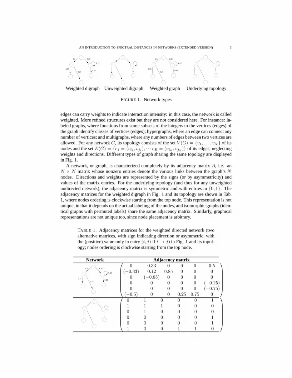
edges can carry weights to indicate interaction intensity:in this case, the network is calledweighted. More refined structures exist but they are not considered here. For instance: la-beled graphs, where functions from some subsets of the integers to the vertices (edges) ofthe graph identify classes of vertices (edges); hypergraphs, where an edge can connect anynumber of vertices; and multigraphs, where any numbers of edges between two vertices areallowed. For any networkG, its topology consists of the setV (G) = {v1, . . . , vN} of itsnodes and the setE(G) = {e1 = (vi1 , vj1), · · · eE = (viE , vjE )} of its edges, neglectingweights and directions. Different types of graph sharing the same topology are displayedin Fig. 1.

A network, or graph, is characterized completely by its adjacency matrixA, i.e. anN × N matrix whose nonzero entries denote the various links between the graph’sNnodes. Directions and weights are represented by the signs (or by asymmetricity) andvalues of the matrix entries. For the underlying topology (and thus for any unweightedundirected network), the adjacency matrix is symmetric andwith entries in{0, 1}. Theadjacency matrices for the weighted digraph in Fig. 1 and itstopology are shown in Tab.1, where nodes ordering is clockwise starting from the top node. This representation is notunique, in that it depends on the actual labeling of the nodes, and isomorphic graphs (iden-tical graphs with permuted labels) share the same adjacencymatrix. Similarly, graphicalrepresentations are not unique too, since node placement isarbitrary.

TABLE 1. Adjacency matrices for the weighted directed network (twoalternative matrices, with sign indicating direction or asymmetric, withthe (positive) value only in entry(i, j) if i → j) in Fig. 1 and its topol-ogy; nodes ordering is clockwise starting from the top node.

Network Adjacency matrix

0.25

0.75

0.5 0.33

0.12

0.85

0 0.33 0 0 0 0.5(−0.33) 0.12 0.85 0 0 0

0 (−0.85) 0 0 0 00 0 0 0 0 (−0.25)0 0 0 0 0 (−0.75)

(−0.5) 0 0 0.25 0.75 0

0 1 0 0 0 11 1 1 0 0 00 1 0 0 0 00 0 0 0 0 10 0 0 0 0 11 0 0 1 1 0

4 GIUSEPPE JURMAN, ROBERTO VISINTAINER, AND CESARE FURLANELLO

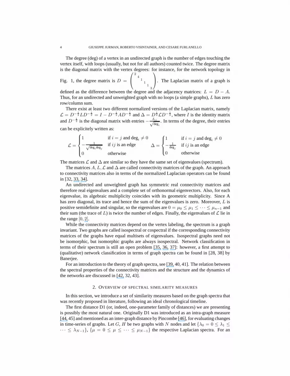
The degree (deg) of a vertex in an undirected graph is the number of edges touching thevertex itself, with loops (usually, but not for all authors)counted twice. The degree matrixis the diagonal matrix with the vertex degrees: for instance, for the network topology in

Fig. 1, the degree matrix isD =

241113

. The Laplacian matrix of a graph is

defined as the difference between the degree and the adjacency matrices:L = D − A.Thus, for an undirected and unweighted graph with no loops (asimple graphs),L has zerorow/column sum.

There exist at least two different normalized versions of the Laplacian matrix, namelyL = D−

1

2LD−1

2 = I −D−1

2AD−1

2 and∆ = D1

2LD−1

2 , whereI is the identity matrixandD−

1

2 is the diagonal matrix with entries− δij√degi

. In terms of the degree, their entries

can be explicitely written as:

L =

1 if i = j and degi 6= 0

− 1√degidegj

if ij is an edge

0 otherwise

∆ =

1 if i = j and degi 6= 0

− 1degj

if ij is an edge

0 otherwise

The matricesL and∆ are similar so they have the same set of eigenvalues (spectrum).The matricesA,L,L and∆ are called connectivity matrices of the graph. An approach

to connectivity matrices also in terms of the normalized Laplacian operators can be foundin [32, 33, 34].

An undirected and unweighted graph has symmetric real connectivity matrices andtherefore real eigenvalues and a complete set of orthonormal eigenvectors. Also, for eacheigenvalue, its algebraic multiplicity coincides with itsgeometric multiplicity. Since Ahas zero diagonal, its trace and hence the sum of the eigenvalues is zero. Moreover,L ispositive semidefinite and singular, so the eigenvalues are0 = µ0 ≤ µ1 ≤ · · · ≤ µn−1 andtheir sum (the trace ofL) is twice the number of edges. Finally, the eigenvalues ofL lie inthe range[0, 2].

While the connectivity matrices depend on the vertex labeling, the spectrum is a graphinvariant. Two graphs are called isospectral or cospectralif the corresponding connectivitymatrices of the graphs have equal multisets of eigenvalues.Isospectral graphs need notbe isomorphic, but isomorphic graphs are always isospectral. Network classification interms of their spectrum is still an open problem [35, 36, 37]:however, a first attempt to(qualitative) network classification in terms of graph spectra can be found in [28, 38] byBanerjee.

For an introduction to the theory of graph spectra, see [39, 40, 41]. The relation betweenthe spectral properties of the connectivity matrices and the structure and the dynamics ofthe networks are discussed in [42, 32, 43].

2. OVERVIEW OF SPECTRAL SIMILARITY MEASURES

In this section, we introduce a set of similarity measures based on the graph spectra thatwas recently proposed in literature, following an ideal chronological timeline.

The first distance D1 (or, indeed, one-parameter family of distances) we are presentingis possibly the most natural one. Originally D1 was introduced as an intra-graph measure[44, 45] and mentioned as an inter-graph distance by Pincombe [46], for evaluating changesin time-series of graphs. LetG, H be two graphs withN nodes and let{λ0 = 0 ≤ λ1 ≤· · · ≤ λN−1}, {µ = 0 ≤ µ ≤ · · · ≤ µN−1} the respective Laplacian spectra. For an

AN INTRODUCTION TO SPECTRAL DISTANCES IN NETWORKS (EXTENDED VERSION) 5

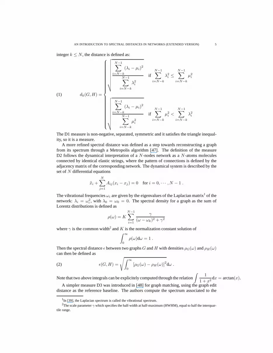
integerk ≤ N , the distance is defined as:

(1) dk(G,H) =

√

√

√

√

√

√

√

√

√

√

N−1∑

i=N−k

(λi − µi)2

N−1∑

i=N−k

λ2i

ifN−1∑

i=N−k

λ2i ≤

N−1∑

i=N−k

µ2i

√

√

√

√

√

√

√

√

√

√

N−1∑

i=N−k

(λi − µi)2

N−1∑

i=N−k

µ2i

ifN−1∑

i=N−k

µ2i <

N−1∑

i=N−k

λ2i

The D1 measure is non-negative, separated, symmetric and itsatisfies the triangle inequal-ity, so it is a measure.

A more refined spectral distance was defined as a step towards reconstructing a graphfrom its spectrum through a Metropolis algorithm [47]. The definition of the measureD2 follows the dynamical interpretation of aN -nodes network as aN -atoms moleculesconnected by identical elastic strings, where the pattern of connections is defined by theadjacency matrix of the corresponding network. The dynamical system is described by theset ofN differential equations

xi +N∑

j=1

Aij(xi − xj) = 0 for i = 0, · · · , N − 1 .

The vibrational frequenciesωi are given by the eigenvalues of the Laplacian matrix1 of thenetwork: λi = ω2

i , with λ0 = ω0 = 0. The spectral density for a graph as the sum ofLorentz distributions is defined as

ρ(ω) = K

N−1∑

i=1

γ

(ω − ωk)2 + γ2

whereγ is the common width2 andK is the normalization constant solution of∫

∞

0

ρ(ω)dω = 1 .

Then the spectral distanceǫ between two graphsG andH with densitiesρG(ω) andρH(ω)can then be defined as

(2) ǫ(G,H) =

√

∫

∞

0

[ρG(ω)− ρH(ω)]2dω .

Note that two above integrals can be explicitely computed through the relation∫

1

1 + x2dx = arctan(x).

A simpler measure D3 was introduced in [48] for graph matching, using the graph editdistance as the reference baseline. The authors compute thespectrum associated to the

1In [39], the Laplacian spectrum is called the vibrational spectrum.2The scale parameterγ which specifies the half-width at half-maximum (HWHM), equal to half the interquar-

tile range.

6 GIUSEPPE JURMAN, ROBERTO VISINTAINER, AND CESARE FURLANELLO

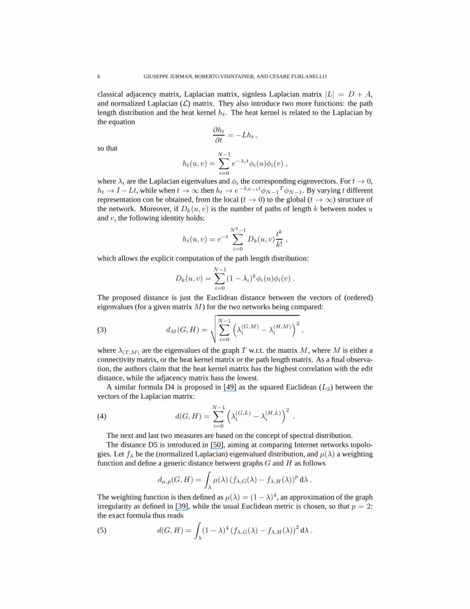
classical adjacency matrix, Laplacian matrix, signless Laplacian matrix|L| = D + A,and normalized Laplacian (L) matrix. They also introduce two more functions: the pathlength distribution and the heat kernelht. The heat kernel is related to the Laplacian bythe equation

∂ht

∂t= −Lht ,

so that

ht(u, v) =

N−1∑

i=0

e−λitφi(u)φi(v) ,

whereλi are the Laplacian eigenvalues andφi the corresponding eigenvectors. Fort → 0,ht → I−Lt, while whent → ∞ thenht → e−λN−1tφN−1

TφN−1. By varyingt differentrepresentation con be obtained, from the local (t → 0) to the global (t → ∞) structure ofthe network. Moreover, ifDk(u, v) is the number of paths of lengthk between nodesuandv, the following identity holds:

ht(u, v) = e−t

N2−1

∑

i=0

Dk(u, v)tk

k!,

which allows the explicit computation of the path length distribution:

Dk(u, v) =N−1∑

i=0

(1− λi)kφi(u)φi(v) .

The proposed distance is just the Euclidean distance between the vectors of (ordered)eigenvalues (for a given matrixM ) for the two networks being compared:

(3) dM (G,H) =

√

√

√

√

N−1∑

i=0

(

λ(G,M)i − λ

(H,M)i

)2

,

whereλ(T,M) are the eigenvalues of the graphT w.r.t. the matrixM , whereM is either aconnectivity matrix, or the heat kernel matrix or the path length matrix. As a final observa-tion, the authors claim that the heat kernel matrix has the highest correlation with the editdistance, while the adjacency matrix hass the lowest.

A similar formula D4 is proposed in [49] as the squared Euclidean (L2) between thevectors of the Laplacian matrix:

(4) d(G,H) =N−1∑

i=0

(

λ(G,L)i − λ

(H,L)i

)2

.

The next and last two measures are based on the concept of spectral distribution.The distance D5 is introduced in [50], aiming at comparing Internet networks topolo-

gies. Letfλ be the (normalized Laplacian) eigenvalued distribution, andµ(λ) a weightingfunction and define a generic distance between graphsG andH as follows

dµ,p(G,H) =

∫

λ

µ(λ) (fλ,G(λ) − fλ,H(λ))p dλ .

The weighting function is then defined asµ(λ) = (1− λ)4, an approximation of the graphirregularity as defined in [39], while the usual Euclidean metric is chosen, so thatp = 2:the exact formula thus reads

(5) d(G,H) =

∫

λ

(1− λ)4 (fλ,G(λ)− fλ,H(λ))2 dλ .

AN INTRODUCTION TO SPECTRAL DISTANCES IN NETWORKS (EXTENDED VERSION) 7

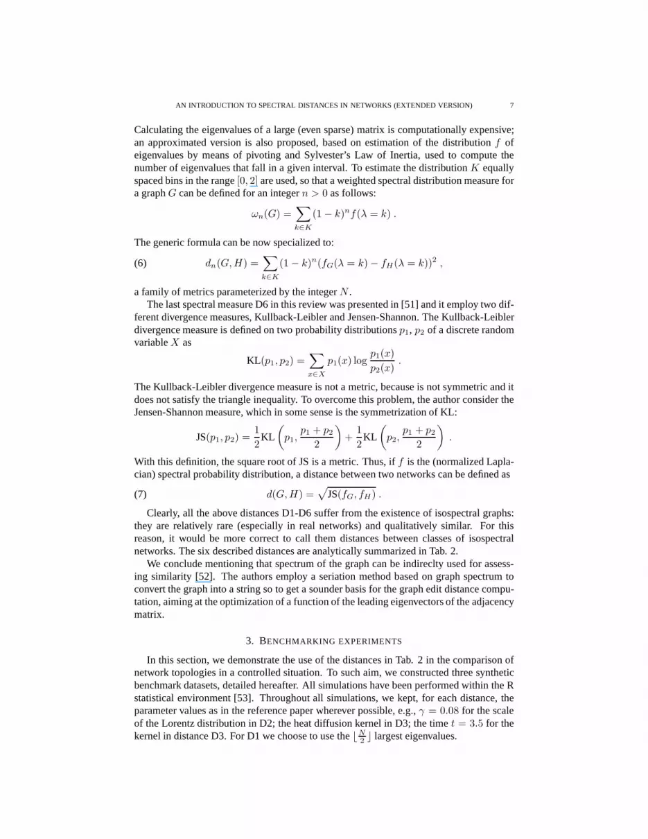
Calculating the eigenvalues of a large (even sparse) matrixis computationally expensive;an approximated version is also proposed, based on estimation of the distributionf ofeigenvalues by means of pivoting and Sylvester’s Law of Inertia, used to compute thenumber of eigenvalues that fall in a given interval. To estimate the distributionK equallyspaced bins in the range[0, 2] are used, so that a weighted spectral distribution measure fora graphG can be defined for an integern > 0 as follows:

ωn(G) =∑

k∈K

(1− k)nf(λ = k) .

The generic formula can be now specialized to:

(6) dn(G,H) =∑

k∈K

(1− k)n(fG(λ = k)− fH(λ = k))2 ,

a family of metrics parameterized by the integerN .The last spectral measure D6 in this review was presented in [51] and it employ two dif-

ferent divergence measures, Kullback-Leibler and Jensen-Shannon. The Kullback-Leiblerdivergence measure is defined on two probability distributionsp1, p2 of a discrete randomvariableX as

KL(p1, p2) =∑

x∈X

p1(x) logp1(x)

p2(x).

The Kullback-Leibler divergence measure is not a metric, because is not symmetric and itdoes not satisfy the triangle inequality. To overcome this problem, the author consider theJensen-Shannon measure, which in some sense is the symmetrization of KL:

JS(p1, p2) =1

2KL

(

p1,p1 + p2

2

)

+1

2KL

(

p2,p1 + p2

2

)

.

With this definition, the square root of JS is a metric. Thus, if f is the (normalized Lapla-cian) spectral probability distribution, a distance between two networks can be defined as

(7) d(G,H) =√

JS(fG, fH) .

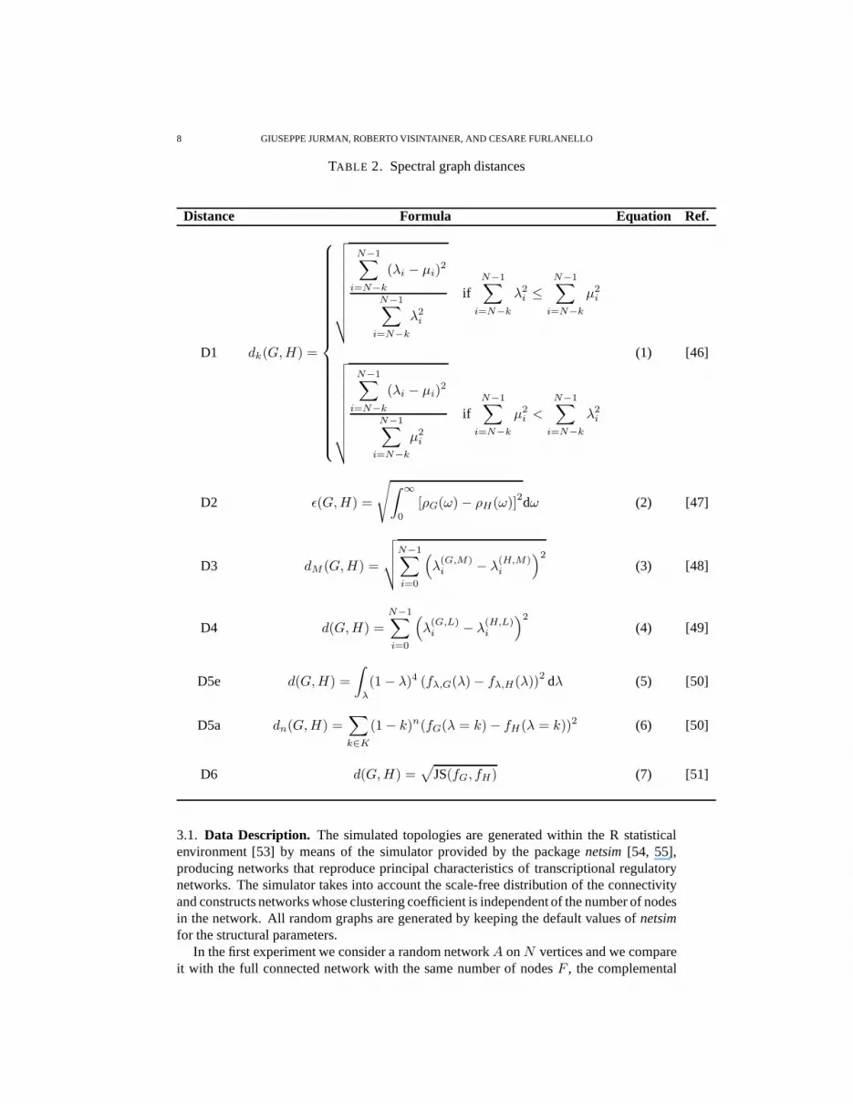
Clearly, all the above distances D1-D6 suffer from the existence of isospectral graphs:they are relatively rare (especially in real networks) and qualitatively similar. For thisreason, it would be more correct to call them distances between classes of isospectralnetworks. The six described distances are analytically summarized in Tab. 2.

We conclude mentioning that spectrum of the graph can be indireclty used for assess-ing similarity [52]. The authors employ a seriation method based on graph spectrum toconvert the graph into a string so to get a sounder basis for the graph edit distance compu-tation, aiming at the optimization of a function of the leading eigenvectors of the adjacencymatrix.

3. BENCHMARKING EXPERIMENTS

In this section, we demonstrate the use of the distances in Tab. 2 in the comparison ofnetwork topologies in a controlled situation. To such aim, we constructed three syntheticbenchmark datasets, detailed hereafter. All simulations have been performed within the Rstatistical environment [53]. Throughout all simulations, we kept, for each distance, theparameter values as in the reference paper wherever possible, e.g.,γ = 0.08 for the scaleof the Lorentz distribution in D2; the heat diffusion kernelin D3; the timet = 3.5 for thekernel in distance D3. For D1 we choose to use the⌊N

2 ⌋ largest eigenvalues.

8 GIUSEPPE JURMAN, ROBERTO VISINTAINER, AND CESARE FURLANELLO

TABLE 2. Spectral graph distances

Distance Formula Equation Ref.

D1 dk(G,H) =

√

√

√

√

√

√

√

√

√

√

N−1∑

i=N−k

(λi − µi)2

N−1∑

i=N−k

λ2i

ifN−1∑

i=N−k

λ2i ≤

N−1∑

i=N−k

µ2i

√

√

√

√

√

√

√

√

√

√

N−1∑

i=N−k

(λi − µi)2

N−1∑

i=N−k

µ2i

ifN−1∑

i=N−k

µ2i <

N−1∑

i=N−k

λ2i

(1) [46]

D2 ǫ(G,H) =

√

∫

∞

0

[ρG(ω)− ρH(ω)]2dω (2) [47]

D3 dM (G,H) =

√

√

√

√

N−1∑

i=0

(

λ(G,M)i − λ

(H,M)i

)2

(3) [48]

D4 d(G,H) =

N−1∑

i=0

(

λ(G,L)i − λ

(H,L)i

)2

(4) [49]

D5e d(G,H) =

∫

λ

(1− λ)4 (fλ,G(λ)− fλ,H(λ))2 dλ (5) [50]

D5a dn(G,H) =∑

k∈K

(1− k)n(fG(λ = k)− fH(λ = k))2 (6) [50]

D6 d(G,H) =√

JS(fG, fH) (7) [51]

3.1. Data Description. The simulated topologies are generated within the R statisticalenvironment [53] by means of the simulator provided by the packagenetsim[54, 55],producing networks that reproduce principal characteristics of transcriptional regulatorynetworks. The simulator takes into account the scale-free distribution of the connectivityand constructs networks whose clustering coefficient is independent of the number of nodesin the network. All random graphs are generated by keeping the default values ofnetsimfor the structural parameters.

In the first experiment we consider a random networkA onN vertices and we compareit with the full connected network with the same number of nodesF , the complemental

AN INTRODUCTION TO SPECTRAL DISTANCES IN NETWORKS (EXTENDED VERSION) 9

A A5 A F

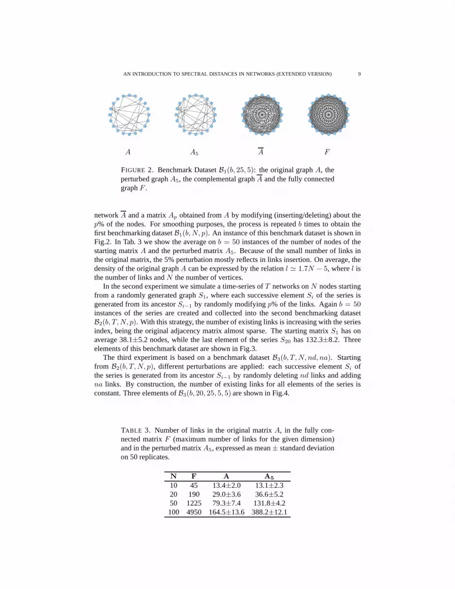
FIGURE 2. Benchmark DatasetB1(b, 25, 5): the original graphA, theperturbed graphA5, the complemental graphA and the fully connectedgraphF .

networkA and a matrixAp obtained fromA by modifying (inserting/deleting) about thep% of the nodes. For smoothing purposes, the process is repeated b times to obtain thefirst benchmarking datasetB1(b,N, p). An instance of this benchmark dataset is shown inFig.2. In Tab. 3 we show the average onb = 50 instances of the number of nodes of thestarting matrixA and the perturbed matrixA5. Because of the small number of links inthe original matrix, the 5% perturbation mostly reflects in links insertion. On average, thedensity of the original graphA can be expressed by the relationl ≃ 1.7N − 5, wherel isthe number of links andN the number of vertices.

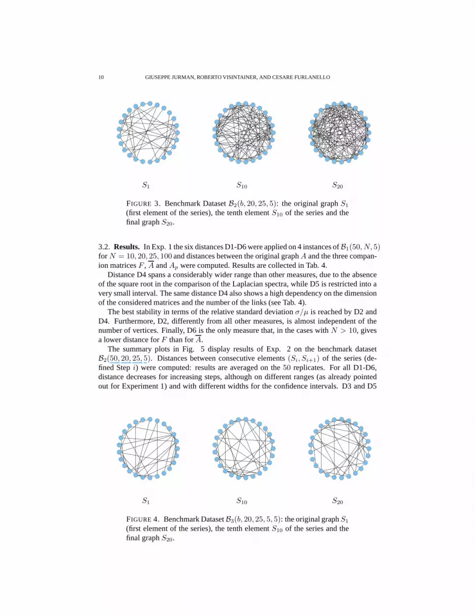
In the second experiment we simulate a time-series ofT networks onN nodes startingfrom a randomly generated graphS1, where each successive elementSi of the series isgenerated from its ancestorSi−1 by randomly modifyingp% of the links. Againb = 50instances of the series are created and collected into the second benchmarking datasetB2(b, T,N, p). With this strategy, the number of existing links is increasing with the seriesindex, being the original adjacency matrix almost sparse. The starting matrixS1 has onaverage 38.1±5.2 nodes, while the last element of the seriesS20 has 132.3±8.2. Threeelements of this benchmark dataset are shown in Fig.3.

The third experiment is based on a benchmark datasetB3(b, T,N, nd, na). Startingfrom B2(b, T,N, p), different perturbations are applied: each successive elementSi ofthe series is generated from its ancestorSi−1 by randomly deletingnd links and addingna links. By construction, the number of existing links for allelements of the series isconstant. Three elements ofB3(b, 20, 25, 5, 5) are shown in Fig.4.

TABLE 3. Number of links in the original matrixA, in the fully con-nected matrixF (maximum number of links for the given dimension)and in the perturbed matrixA5, expressed as mean± standard deviationon 50 replicates.

N F A A5

10 45 13.4±2.0 13.1±2.320 190 29.0±3.6 36.6±5.250 1225 79.3±7.4 131.8±4.2100 4950 164.5±13.6 388.2±12.1

10 GIUSEPPE JURMAN, ROBERTO VISINTAINER, AND CESARE FURLANELLO

S1 S10 S20

FIGURE 3. Benchmark DatasetB2(b, 20, 25, 5): the original graphS1

(first element of the series), the tenth elementS10 of the series and thefinal graphS20.

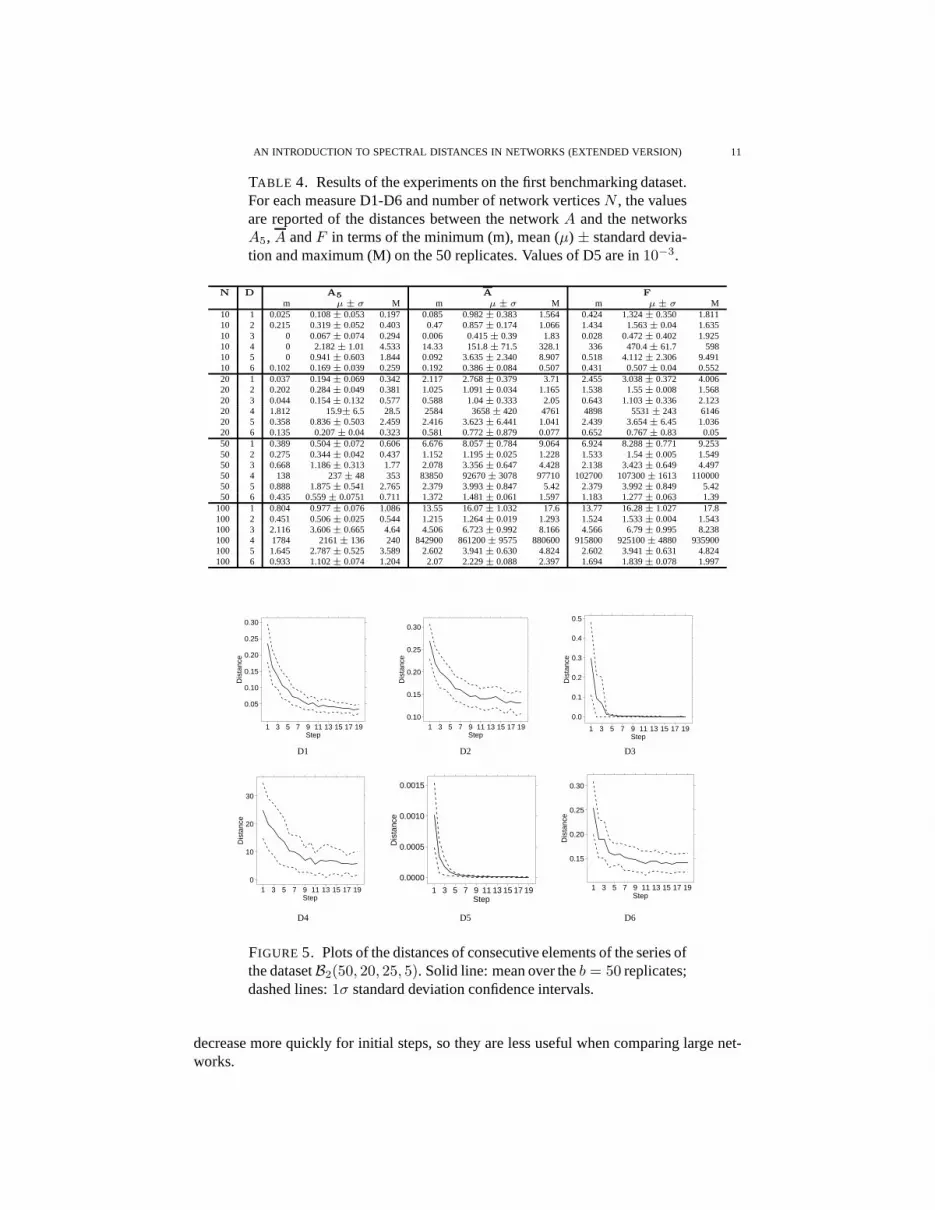
3.2. Results. In Exp. 1 the six distances D1-D6 were applied on 4 instances of B1(50, N, 5)for N = 10, 20, 25, 100 and distances between the original graphA and the three compan-ion matricesF , A andAp were computed. Results are collected in Tab. 4.

Distance D4 spans a considerably wider range than other measures, due to the absenceof the square root in the comparison of the Laplacian spectra, while D5 is restricted into avery small interval. The same distance D4 also shows a high dependency on the dimensionof the considered matrices and the number of the links (see Tab. 4).

The best stability in terms of the relative standard deviationσ/µ is reached by D2 andD4. Furthermore, D2, differently from all other measures, is almost independent of thenumber of vertices. Finally, D6 is the only measure that, in the cases withN > 10, givesa lower distance forF than forA.

The summary plots in Fig. 5 display results of Exp. 2 on the benchmark datasetB2(50, 20, 25, 5). Distances between consecutive elements(Si, Si+1) of the series (de-fined Stepi) were computed: results are averaged on the50 replicates. For all D1-D6,distance decreases for increasing steps, although on different ranges (as already pointedout for Experiment 1) and with different widths for the confidence intervals. D3 and D5

S1 S10 S20

FIGURE 4. Benchmark DatasetB3(b, 20, 25, 5, 5): the original graphS1

(first element of the series), the tenth elementS10 of the series and thefinal graphS20.

AN INTRODUCTION TO SPECTRAL DISTANCES IN NETWORKS (EXTENDED VERSION) 11

TABLE 4. Results of the experiments on the first benchmarking dataset.For each measure D1-D6 and number of network verticesN , the valuesare reported of the distances between the networkA and the networksA5, A andF in terms of the minimum (m), mean (µ) ± standard devia-tion and maximum (M) on the 50 replicates. Values of D5 are in10−3.

N D A5 A F

m µ ± σ M m µ ± σ M m µ ± σ M10 1 0.025 0.108± 0.053 0.197 0.085 0.982± 0.383 1.564 0.424 1.324± 0.350 1.81110 2 0.215 0.319± 0.052 0.403 0.47 0.857± 0.174 1.066 1.434 1.563± 0.04 1.63510 3 0 0.067± 0.074 0.294 0.006 0.415± 0.39 1.83 0.028 0.472± 0.402 1.92510 4 0 2.182± 1.01 4.533 14.33 151.8± 71.5 328.1 336 470.4± 61.7 59810 5 0 0.941± 0.603 1.844 0.092 3.635± 2.340 8.907 0.518 4.112± 2.306 9.49110 6 0.102 0.169± 0.039 0.259 0.192 0.386± 0.084 0.507 0.431 0.507± 0.04 0.55220 1 0.037 0.194± 0.069 0.342 2.117 2.768± 0.379 3.71 2.455 3.038± 0.372 4.00620 2 0.202 0.284± 0.049 0.381 1.025 1.091± 0.034 1.165 1.538 1.55± 0.008 1.56820 3 0.044 0.154± 0.132 0.577 0.588 1.04± 0.333 2.05 0.643 1.103± 0.336 2.12320 4 1.812 15.9± 6.5 28.5 2584 3658± 420 4761 4898 5531± 243 614620 5 0.358 0.836± 0.503 2.459 2.416 3.623± 6.441 1.041 2.439 3.654± 6.45 1.03620 6 0.135 0.207± 0.04 0.323 0.581 0.772± 0.879 0.077 0.652 0.767± 0.83 0.0550 1 0.389 0.504± 0.072 0.606 6.676 8.057± 0.784 9.064 6.924 8.288± 0.771 9.25350 2 0.275 0.344± 0.042 0.437 1.152 1.195± 0.025 1.228 1.533 1.54± 0.005 1.54950 3 0.668 1.186± 0.313 1.77 2.078 3.356± 0.647 4.428 2.138 3.423± 0.649 4.49750 4 138 237± 48 353 83850 92670± 3078 97710 102700 107300± 1613 11000050 5 0.888 1.875± 0.541 2.765 2.379 3.993± 0.847 5.42 2.379 3.992± 0.849 5.4250 6 0.435 0.559± 0.0751 0.711 1.372 1.481± 0.061 1.597 1.183 1.277± 0.063 1.39

100 1 0.804 0.977± 0.076 1.086 13.55 16.07± 1.032 17.6 13.77 16.28± 1.027 17.8100 2 0.451 0.506± 0.025 0.544 1.215 1.264± 0.019 1.293 1.524 1.533± 0.004 1.543100 3 2.116 3.606± 0.665 4.64 4.506 6.723± 0.992 8.166 4.566 6.79± 0.995 8.238100 4 1784 2161± 136 240 842900 861200± 9575 880600 915800 925100± 4880 935900100 5 1.645 2.787± 0.525 3.589 2.602 3.941± 0.630 4.824 2.602 3.941± 0.631 4.824100 6 0.933 1.102± 0.074 1.204 2.07 2.229± 0.088 2.397 1.694 1.839± 0.078 1.997

Step

Dis

tanc

e

0.05

0.10

0.15

0.20

0.25

0.30

1 3 5 7 9 11 13 15 17 19Step

Dis

tanc

e

0.10

0.15

0.20

0.25

0.30

1 3 5 7 9 11 13 15 17 19Step

Dis

tanc

e

0.0

0.1

0.2

0.3

0.4

0.5

1 3 5 7 9 11 13 15 17 19

D1 D2 D3

Step

Dis

tanc

e

0

10

20

30

1 3 5 7 9 11 13 15 17 19Step

Dis

tanc

e

0.0000

0.0005

0.0010

0.0015

1 3 5 7 9 11 13 15 17 19Step

Dis

tanc

e

0.15

0.20

0.25

0.30

1 3 5 7 9 11 13 15 17 19

D4 D5 D6

FIGURE 5. Plots of the distances of consecutive elements of the series ofthe datasetB2(50, 20, 25, 5). Solid line: mean over theb = 50 replicates;dashed lines:1σ standard deviation confidence intervals.

decrease more quickly for initial steps, so they are less useful when comparing large net-works.

12 GIUSEPPE JURMAN, ROBERTO VISINTAINER, AND CESARE FURLANELLO

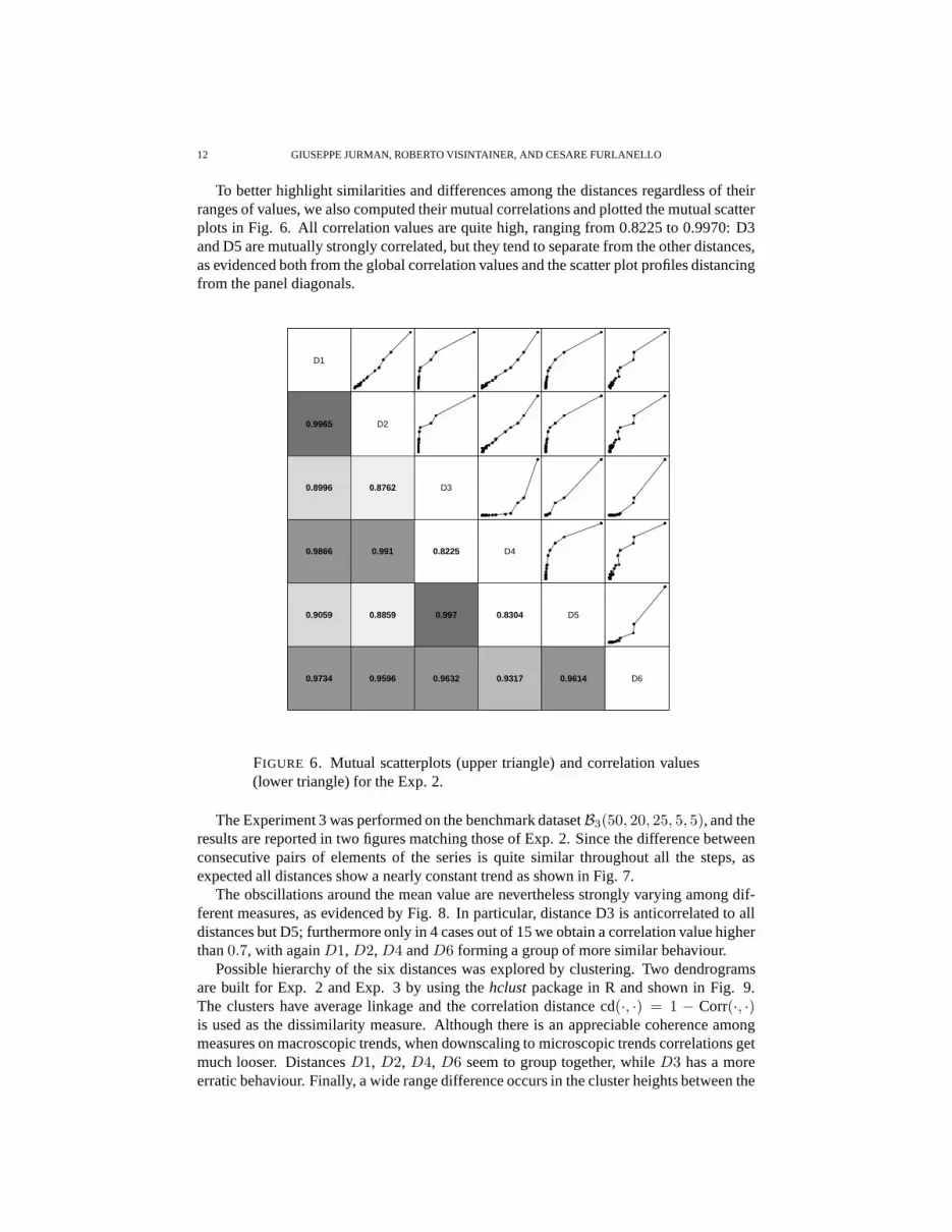
To better highlight similarities and differences among thedistances regardless of theirranges of values, we also computed their mutual correlations and plotted the mutual scatterplots in Fig. 6. All correlation values are quite high, ranging from 0.8225 to 0.9970: D3and D5 are mutually strongly correlated, but they tend to separate from the other distances,as evidenced both from the global correlation values and thescatter plot profiles distancingfrom the panel diagonals.

D1

0.9965 D2

0.8996 0.8762 D3

0.9866 0.991 0.8225 D4

0.9059 0.8859 0.997 0.8304 D5

0.9734 0.9596 0.9632 0.9317 0.9614 D6

FIGURE 6. Mutual scatterplots (upper triangle) and correlation values(lower triangle) for the Exp. 2.

The Experiment 3 was performed on the benchmark datasetB3(50, 20, 25, 5, 5), and theresults are reported in two figures matching those of Exp. 2. Since the difference betweenconsecutive pairs of elements of the series is quite similarthroughout all the steps, asexpected all distances show a nearly constant trend as shownin Fig. 7.

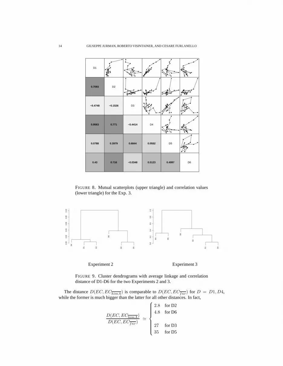
The obscillations around the mean value are nevertheless strongly varying among dif-ferent measures, as evidenced by Fig. 8. In particular, distance D3 is anticorrelated to alldistances but D5; furthermore only in 4 cases out of 15 we obtain a correlation value higherthan0.7, with againD1, D2, D4 andD6 forming a group of more similar behaviour.

Possible hierarchy of the six distances was explored by clustering. Two dendrogramsare built for Exp. 2 and Exp. 3 by using thehclustpackage in R and shown in Fig. 9.The clusters have average linkage and the correlation distance cd(·, ·) = 1 − Corr(·, ·)is used as the dissimilarity measure. Although there is an appreciable coherence amongmeasures on macroscopic trends, when downscaling to microscopic trends correlations getmuch looser. DistancesD1, D2, D4, D6 seem to group together, whileD3 has a moreerratic behaviour. Finally, a wide range difference occursin the cluster heights between the

AN INTRODUCTION TO SPECTRAL DISTANCES IN NETWORKS (EXTENDED VERSION) 13

Step

Dis

tanc

e

0.04

0.05

0.06

0.07

0.08

0.09

1 3 5 7 9 11 13 15 17 19Step

Dis

tanc

e

0.14

0.16

0.18

0.20

0.22

0.24

1 3 5 7 9 11 13 15 17 19Step

Dis

tanc

e

0.0

0.1

0.2

0.3

1 3 5 7 9 11 13 15 17 19

D1 D2 D3

Step

Dis

tanc

e

1

2

3

4

1 3 5 7 9 11 13 15 17 19

Step

Dis

tanc

e

0e+00

2e−04

4e−04

6e−04

8e−04

1 3 5 7 9 11 13 15 17 19Step

Dis

tanc

e

0.12

0.14

0.16

0.18

0.20

1 3 5 7 9 11 13 15 17 19

D4 D5 D6

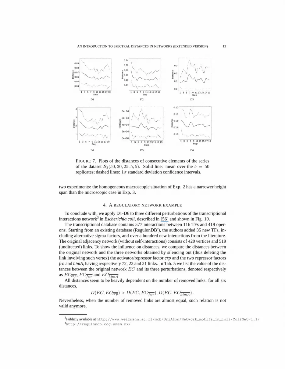
FIGURE 7. Plots of the distances of consecutive elements of the seriesof the datasetB3(50, 20, 25, 5, 5). Solid line: mean over theb = 50replicates; dashed lines:1σ standard deviation confidence intervals.

two experiments: the homogeneous macroscopic situation ofExp. 2 has a narrower heightspan than the microscopic case in Exp. 3.

4. A REGULATORY NETWORK EXAMPLE

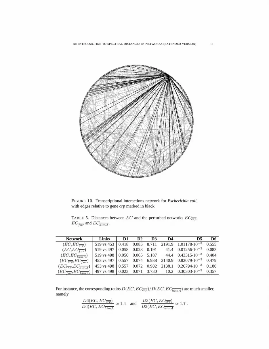
To conclude with, we apply D1-D6 to three different perturbations of the transcriptionalinteractions network3 in Escherichia coli, described in [56] and shown in Fig. 10.

The transcriptional database contains 577 interactions between 116 TFs and 419 oper-ons. Starting from an existing database (RegulonDB4), the authors added 35 new TFs, in-cluding alternative sigma factors, and over a hundred new interactions from the literature.The original adjacency network (without self-interactions) consists of 420 vertices and 519(undirected) links. To show the influence on distances, we compare the distances betweenthe original network and the three networks obtained by silencing out (thus deleting thelink involving such vertex) the activator/repressor factor crp and the two repressor factorsfrn andhimA, having respectively 72, 22 and 21 links. In Tab. 5 we list thevalue of the dis-tances between the original networkEC and its three perturbations, denoted respectivelyasECcrp, ECfnr andEChimA.

All distances seem to be heavily dependent on the number of removed links: for all sixdistances,

D(EC,ECcrp) > D(EC,ECfnr), D(EC,EChimA) .

Nevertheless, when the number of removed links are almost equal, such relation is notvalid anymore.

3Publicly available athttp://www.weizmann.ac.il/mcb/UriAlon/Network_motifs_in_coli/ColiNet-1.1/4http://regulondb.ccg.unam.mx/

14 GIUSEPPE JURMAN, ROBERTO VISINTAINER, AND CESARE FURLANELLO

D1

0.7093 D2

−0.4748 −0.1526 D3

0.9563 0.771 −0.4414 D4

0.0788 0.3979 0.6844 0.0552 D5

0.43 0.716 −0.0348 0.5123 0.4997 D6

FIGURE 8. Mutual scatterplots (upper triangle) and correlation values(lower triangle) for the Exp. 3.

D4

D1

D2

D6

D3

D5

0.00

0.02

0.04

0.06

0.08

0.10

D3

D5

D6

D2

D1

D4

0.0

0.2

0.4

0.6

0.8

1.0

Experiment 2 Experiment 3

FIGURE 9. Cluster dendrograms with average linkage and correlationdistance of D1-D6 for the two Experiments 2 and 3.

The distanceD(EC,EChimA) is comparable toD(EC,ECfnr) for D = D1, D4,while the former is much bigger than the latter for all other distances. In fact,

D(EC,EChimA)

D(EC,ECfnr)≃

2.8 for D2

4.8 for D6

27 for D3

35 for D5

AN INTRODUCTION TO SPECTRAL DISTANCES IN NETWORKS (EXTENDED VERSION) 15

FIGURE 10. Transcriptional interactions network forEscherichia coli,with edges relative to genecrp marked in black.

TABLE 5. Distances betweenEC and the perturbed networksECcrp,ECfnr andEChimA.

Network Links D1 D2 D3 D4 D5 D6(EC,ECcrp) 519 vs 453 0.418 0.085 8.711 2191.9 1.01178·10−3 0.555(EC,ECfnr) 519 vs 497 0.058 0.023 0.191 41.4 0.01256·10−3 0.083

(EC,EChimA) 519 vs 498 0.056 0.065 5.187 44.4 0.43315·10−3 0.404(ECcrp,ECfnr) 453 vs 497 0.557 0.074 6.938 2140.9 0.82079·10−3 0.479

(ECcrp,EChimA) 453 vs 498 0.557 0.072 0.982 2138.1 0.26794·10−3 0.180(ECfnr,EChimA) 497 vs 498 0.023 0.071 3.730 10.2 0.30303·10−3 0.357

For instance, the corresponding ratiosD(EC,ECcrp)/D(EC,EChimA) are much smaller,namely

D6(EC,ECcrp)

D6(EC,EChimA

≃ 1.4 andD3(EC,ECcrp)

D3(EC,EChimA

≃ 1.7 .

16 GIUSEPPE JURMAN, ROBERTO VISINTAINER, AND CESARE FURLANELLO

TABLE 6. Natural logarithm of the size of the automorphism group ofthe original and the perturbed networks

Network G log(|Aut(G)|) max{λi}EC 330.0173 73.021

ECcrp 377.5827 27.015ECfnr 341.4692 73.019EChimA 347.4488 73.020

A possible explanation is in the quite different structure of the two networksECfnr andEChimA, although being obtained silencing out almost the same number of links from theoriginal network.

The intrinsic structural difference betweenECfnr andEChimA is indeed highlightedby the remarkable variation in the size of the respective group of automorphisms as shownin Tab. 6. For instance, the structure ofEChimA is almoste347.4488−341.4692 ≃ 400 timesmore symmetric thanECfnr. From this point of view, spectral distances can greatly helpin analyzing subtle differences between networks where more classical methods are nothelping much. As an example, the leading Laplacian eigenvalue is commonly used whennetwork structure, because it is a good indicator of the stability and the local dynamics[57]. For instance, in this particular example, this value is of no help, as indicated in Tab. 6,sinceEC, ECfnr andEChimA have essentially the same leading eigenvalue; neverthelessthe spectral distances, encoding information coming from the whole spectrum, can betterseparate very similar networks. Summarizing the observations following the experimentson synthetic data and the results in Tab. 5, we can conclude proposingD2 as the morereliable metric, both in terms of stability and robustness in terms of being less prone to oddbehaviours.

ACKNOWLEDGEMENTS

The authors acknowledge funding by the European Union FP7 Project HiperDART andby the Italian Ministry of Health Project ISITAD (RF 2007 conv. 42). The authors aregrateful to Samantha Riccadonna for her help with the R programming language.

REFERENCES

[1] S. Boccaletti, V. Latora, Y. Moreno, M. Chavez, and D.-U.Hwang. Complex networks: Structure anddynamics.Phys. Rep., 424(4–5):175–308, 2006.

[2] S.H. Strogatz. Exploring complex networks.Nature, 410:268–276, 2001.[3] B. MacArthur, R.J. Sánchez-García, and J. Anderson. Symmetry in complex networks.Discrete Appl. Math.,

156(18):3525–3531, 2008.[4] R. Albert and A.L. Barabási. Statistical mechanics of complex networks.Rev. Mod. Phys., 74:47, 2002.[5] M.E.J. Newman. The Structure and Function of Complex Networks.SIAM Review, 45:167–256, 2003.[6] D. Liben-Nowell. An Algorithmic Approach to Social Networks. PhD thesis, Massachusetts Institute of

Technology, 2005.[7] S.N. Dorogovtsev, A.V. Goltsev, and J.F.F. Mendes. Critical phenomena in complex networks.Rev. Mod.

Phys., 80(4):1275–1335, 2008.[8] A. Goldenberg, A.X. Zheng, S.E. Fienberg, and E.M. Airoldi. A Survey of Statistical Network Models.

Foundations and Trends in Machine Learning, 2(2):129–233, 2009.[9] V. Lacroix, L. Cottret, P. Thébault, and M.F. Sagot. An introduction to metabolic networks and their struc-

tural analysis.IEEE/ACM Trans. Comput. Biol. Bioinform., 5(4):594–617, 2008.[10] A.P. Cootes, S.H. Muggleton, and M.J.E. Sternberg. TheIdentification of Similarities between Biological

Networks: Application to the Metabolome and Interactome.J. Mol. Biol., 369:1126–1139, 2007.

AN INTRODUCTION TO SPECTRAL DISTANCES IN NETWORKS (EXTENDED VERSION) 17

[11] A. Vazquez, A. Flammini, A. Maritan, and A. Vespignani.Global protein function prediction from protein-protein interaction networks.Nat. Biotechnol., 21:697–700, 2003.

[12] R. Sharan and T. Ideker. Modeling cellular machinery through biological network comparison.Nat. Biotech-nol., 24(4):427–433, 2006.

[13] F. He, R. Balling, and A.-P. Zeng. Reverse engineering and verification of gene networks.J. Biotechnol,144:190–203, 2009.

[14] D. Marbach, R.J. Prill, T. Schaffter, C. Mattiussi, D. Floreano, and G. Stolovitzky. Revealing strengths andweaknesses of methods for gene network inference.PNAS, 107(14):6286–6291, 2010.

[15] W.-P. Lee and W.-S. Tzou. Computational methods for discovering gene networks from expression data.Briefings Bioinf., 10(4):408–423, 2009.

[16] O. Tercieux and V. Vannetelbosch. A characterization of stochastically stable networks.Int. J. Game Theory,34:351–369, 2006.

[17] A. Pomerance, E. Ott, M. Girvan, and W. Losert. The effect of network topology on the stability of discretestate models of genetic control.PNAS, 106(20):8209–8214, 2009.

[18] G. Jurman, S. Merler, A. Barla, S. Paoli, A. Galea, and C.Furlanello. Algebraic stability indicators forranked lists in molecular profiling.Bioinformatics, 24(2):258–264, 2008.

[19] L. da F. Costa, F.A. Rodrigues, G. Travieso, and P.R. Villas Boas. Characterization of complex networks: Asurvey of measurements.Adv. Phys., 56(1):167–202, 2007.

[20] B.D. MacArthur and R.J. Sánchez-García. Spectral characteristics of network redundancy.Phys. Rev. E,80:026117, 2009.

[21] L. da F. Costa and R.F.S. Andrade. What are the best concentric descriptors for complex networks?New J.Phys., 9:311, 2007.

[22] R.C. Entringer, D.E. Jackson, and D.A. Snyder. Distance in graphs.Czech. Math. J., 26(2):283–296, 1976.[23] O. Shanker. Defining dimension of a complex network.Mod. Phys. Lett. B, 21(6):321–326, 2007.[24] O. Shanker. Graph zeta function and dimension of complex network.Mod. Phys. Lett. B, 21(11):639–644,

2007.[25] R. Milo, S. Shen-Orr, S. Itzkovitz, N. Kashtan, D. Chklovskii, and U. Alon. Network Motifs: Simple

Building Blocks of Complex Networks.Science, 298(5594):824–827, 2002.[26] H. Bunke. On a relation between graph edit distance and maximum common subgraph.Pattern Recognition

Letters, 18:689–694, 1997.[27] S.E. Ahnert, D. Garlaschelli, T.M.A. Fink, and G. Caldarelli. Applying weighted network measures to

microarray distance matrices.J. Phys. A: Math. Theor., 41:224011, 2008.[28] A. Banerjee and J. Jost. Spectral plot properties: towards a qualitative classification of networks.Networks

and heterogeneous media, 3(2):395–411, 2008.[29] A. Banerjee and J. Jost. Spectral plots and the representation and interpretation of biological data.Theory

in Biosciences, 126(1):1431–7613 (Print) 1611–7530 (Online), 2007.[30] A. Banerjee and J. Jost. Graph spectra as a systematic tool in computational biology.Discrete Appl. Math.,

157(10):2425–2431, 2009.[31] G.J. Rodgers, K. Austin, B. Kahng, and D. Kim. Eigenvalue spectra of complex networks.Journal of Physics

A: Mathematical and General, 38(43):9431, 2005.[32] J. Jost. Dynamical Networks. In J. Feng, J. Jost, and M. Qian, editors,Networks: From Biology to Theory,

pages 35–64. Springer-Verlag, 2007.[33] A. Banerjee and J. Jost. On the spectrum of the normalized graph Laplacian.Linear Algebra Appl.,

428:3015–3022, 2008.[34] A. Banerjee.The Spectrum of the Graph Laplacian as a Tool for Analyzing Structure and Evolution of

Networks. PhD thesis, University of Leipzig, 2008.[35] E.R. van Dam and W.H. Haemers. Which graphs are determined by their spectrum?Linear Algebra Appl.,

373:241–272, 2003.[36] W. Wang and C.-X. Xu. A sufficient condition for a family of graphs being determined by their generalized

spectra.Eur. J. Combin., 27:826–840, 2006.[37] W. Wang and C.-X. Xu. On the asymptotic behavior of graphs determined by their generalized spectra.

Discrete Math., 310:70–76, 2010.[38] A. Banerjee and J. Jost. Spectral characterization of network structure and dynamics. In N. Ganguly,

A. Deutsch, and A. Mukherjee, editors,Dynamics On and Of Complex Networks: Applications to Biol-ogy, Computer Science, and the Social Sciences, pages 117–132. Springer-Verlag, 2009.

[39] F. Chung.Spectral Graph Theory. American Mathematical Society, 1997.[40] D. Cvetkovic, P. Rowlinson, and S. Simic. An Introduction to the Theory of Graph Spectra. Cambridge

University Press, 2010.

18 GIUSEPPE JURMAN, ROBERTO VISINTAINER, AND CESARE FURLANELLO

[41] A.E. Brouwer and W.H. Haemers. Spectra of graphs. Dept.of Math., Techn. Univ. Eindhoven, 2010.[42] J. Jost and M.P. Joy. Evolving Networks with distance preferences.Phys. Rev. E, 66:036126, 2002.[43] J.A. Almendral and A. Díaz-Guilera. Dynamical and spectral properties of complex networks.New J. Phys.,

9:187, 2007.[44] D. Jakobson and I. Rivin. Extremal metrics on graphs, I.Forum Math., 14(1):147–163, 2002.[45] S. Bacle.Extremal metrics on graphs and manifold. PhD thesis, McGill University, 2005.[46] B. Pincombe. Detecting changes in time series of network graphs using minimum mean squared error and

cumulative summation. In W. Read and A.J. Roberts, editors,Proc. of the 13th Biennial ComputationalTechniques and Applications Conference, CTAC-2006, pages C450–C473, 2007.

[47] M. Ipsen and A.S. Mikhailov. Evolutionary reconstruction of networks.Phys. Rev. E, 66(4):046109, 2002.[48] P. Zhu and R.C. Wilson. A study of graph spectra for comparing graphs. In W. Clocksin, A. Fitzgibbon, and

P. Torr, editors,Proc. of the 16-th British Machine Vision Conference, 2005.[49] F. Comellas and J. Diaz-Lopez. Spectral reconstruction of complex networks.Physica A, 387:6436–6442,

2008.[50] D. Fay, H. Haddadi, A.W. Moore, R. Mortier, S. Uhlig, andA. Jamakovic. A weighted spectrum metric for

comparison of Internet topologies.SIGMETRICS Perform. Eval. Rev., 37(3):67–72, 2009.[51] A. Banerjee. Structural distance and evolutionary relationship of networks. arXiv:0807.3185], 2009.[52] A. Robles-Kelly and E.R. Hancock. Edit Distance From Graph Spectra. InProc. of the Ninth IEEE Interna-

tional Conference on Computer Vision, ICCV03, page 234. IEEE Computer Society, 2003.[53] R Development Core Team.R: A Language and Environment for Statistical Computing. R Foundation for

Statistical Computing, Vienna, Austria, 2009. ISBN 3-900051-07-0.[54] B. Di Camillo. netsim: Gene network simulator, 2007. R package version 1.1.[55] B. Di Camillo, G. Toffolo, and C. Cobelli. A Gene NetworkSimulator to Assess Reverse Engineering

Algorithms.Ann. N.Y. Acad. Sci., 1158:125–142, 2009.[56] S.S. Shen-Orr, R. Milo, S. Mangan, and U. Alon. Network motifs in the transcriptional regulation network

of Escherichia coli.Nat. Genet., 31:64–68, 2002.[57] R. Steuer and G. Zamora Lopez. Global network properties. In B.H. Junker and F. Schreiber, editors,Anal-

ysis of biological networks, pages 31–64. Wiley, 2008.

FONDAZIONE BRUNO KESSLER, TRENTO, ITALY

E-mail address: jurman@fbk.eu

FONDAZIONE BRUNO KESSLER ANDDISI UNIVERSITY OF TRENTO, TRENTO, ITALY

E-mail address: visintainer@fbk.eu

FONDAZIONE BRUNO KESSLER, TRENTO, ITALY

E-mail address: furlan@fbk.eu