
A Statistical Model for SimulatingSolar Intensity in New Jersey
Henry R. Chai
Advisor: Warren B. Powell
June 2014
Submitted in partial fulfillment
of the requirements for the degree of
Bachelor of Science in Engineering
Department of Operations Research and Financial Engineering
Princeton University

I hereby declare that I am the sole author of this thesis.
I authorize Princeton University to lend this thesis to other institutions or individuals for the
purpose of scholarly research.
Henry R. Chai
I further authorize Princeton University to reproduce this thesis by photocopying or by other
means, in total or in part, at the request of other institutions or individuals for the purpose of
scholarly research.
Henry R. Chai
i

Abstract
This thesis is concerned with the construction of a simulator for solar energy generation lev-
els at 24 solar generation plants in New Jersey as well as a comparison of the profitability of
grid-level and plant-level storage cells. The simulator is statistical in that it is based off of historical
data; specifically the simulator uses ARIMA and/or ARMA time series models to generate solar
energy generation quantities. The quality of the simulator is assessed by comparing the cumulative
distribution functions of the simulated and the actual total daily solar energy generations. The
simulator is then used to compare the profitability of two scenarios for the integration of storage
into the electricity grid: the first scenario considered is grid-level storage i.e. a single, massive
battery while the second scenario considered is generation plant-level storage i.e. a smaller battery
at every solar energy generation plant. The results of the simulation suggest that plant-level storage
is a more profitable investment than a single grid-level storage cell.
ii

Acknowledgements
I would like to thank Professor Powell for guiding me through not only this work but
also for his guidance during my summer as an intern in his PENSA laboratory. His patience and
knowledgeable advice on how to progress proved invaluable to this work.
In addition, other members of the PENSA lab proved incredibly helpful along the way: Dr.
Hugo Simao helped me with this work and advised me closely during my time as an intern in
the PENSA lab; specifically Professor Simao helped me with accessing and processing the data
required for this work as well as helping me understand the way PJM functions. Dr. Belgacem
Bouzaiene-Ayari kept me on task by requiring weekly updates. The weekly updates proved to be
incredibly useful when it came down to writing the thesis and I am very grateful to him for his
weekly reminders.
Lastly, I’d like to thank my friends for helping me keep pace with my work and generally
keeping me sane during this whole process. They provided constant encouragement, useful
feedback and strong support when I was stressed out. I would like to thank Jess Hao in particular
for being infinitely supportive, proofreading this thesis and giving me lots of great constructive
criticism.
iii

To my Mom and Dad:
Thanks for Everything
iv

Contents
1. Introduction 1
1.1. PJM and PSE&G . . . . . . . . . . . . . . . . . . . . . . . . . . . . . . . . . . . . . . . . 3
1.2. Renewable Energy and Storage . . . . . . . . . . . . . . . . . . . . . . . . . . . . . . . . 4
1.3. Thesis Overview . . . . . . . . . . . . . . . . . . . . . . . . . . . . . . . . . . . . . . . . 6
2. Models and Methods 7
2.1. ARIMA and ARMA Models . . . . . . . . . . . . . . . . . . . . . . . . . . . . . . . . . 7
2.1.1. Literature Review . . . . . . . . . . . . . . . . . . . . . . . . . . . . . . . . . . . 8
2.1.2. Model Selection . . . . . . . . . . . . . . . . . . . . . . . . . . . . . . . . . . . . 8
2.2. Dynamic Programs and Approximate Dynamic Programming . . . . . . . . . . . . . 10
2.2.1. State Variable . . . . . . . . . . . . . . . . . . . . . . . . . . . . . . . . . . . . . . 10
2.2.2. Decision Variables . . . . . . . . . . . . . . . . . . . . . . . . . . . . . . . . . . . 11
2.2.3. Model Constraints . . . . . . . . . . . . . . . . . . . . . . . . . . . . . . . . . . . 11
2.2.4. Exogenous Information . . . . . . . . . . . . . . . . . . . . . . . . . . . . . . . . 12
2.2.5. Transition and Objective Function . . . . . . . . . . . . . . . . . . . . . . . . . . 12
2.2.6. Approximate Dynamic Programming . . . . . . . . . . . . . . . . . . . . . . . . 12
3. Sources of Data 14
3.1. Solar Energy Generation Data . . . . . . . . . . . . . . . . . . . . . . . . . . . . . . . . 14
3.2. PJM Local Marginal Price Data . . . . . . . . . . . . . . . . . . . . . . . . . . . . . . . . 15
4. Solar Generation Simulator and Dynamic Program 16
4.1. Solar Generation Simulator Methodology . . . . . . . . . . . . . . . . . . . . . . . . . 16
4.2. Solar Energy Model . . . . . . . . . . . . . . . . . . . . . . . . . . . . . . . . . . . . . . 18
4.2.1. Baseline Model Construction . . . . . . . . . . . . . . . . . . . . . . . . . . . . . 19
4.2.2. Sample Offset Calculation . . . . . . . . . . . . . . . . . . . . . . . . . . . . . . 20
4.2.3. CDF Construction and Z-Score Calculation . . . . . . . . . . . . . . . . . . . . 21
v

4.2.4. ARIMA Model Fitting . . . . . . . . . . . . . . . . . . . . . . . . . . . . . . . . . 23
4.2.5. Conversion to Solar Generation Values . . . . . . . . . . . . . . . . . . . . . . . 24
4.3. The Solar Energy and Storage Dynamic Program . . . . . . . . . . . . . . . . . . . . . 25
5. Results and Discussion 28
5.1. Solar Generation Simulator Results . . . . . . . . . . . . . . . . . . . . . . . . . . . . . 28
5.2. Simulator Output Assessment . . . . . . . . . . . . . . . . . . . . . . . . . . . . . . . . 30
5.3. Dynamic Programming Results . . . . . . . . . . . . . . . . . . . . . . . . . . . . . . . 32
6. Conclusions and Further Research 49
6.1. Physical Constraints of the Storage Model . . . . . . . . . . . . . . . . . . . . . . . . . 49
6.2. Refining the Solar Model . . . . . . . . . . . . . . . . . . . . . . . . . . . . . . . . . . . 50
6.3. Final Remarks . . . . . . . . . . . . . . . . . . . . . . . . . . . . . . . . . . . . . . . . . 51
References 52
Appendix: Code Overview 54
vi

List of Figures
1 US Added PV Capacity from 2010 to 2013 . . . . . . . . . . . . . . . . . . . . . . . . 1
2 Estimated Technical Potential for Utility-Scale Photovolatics . . . . . . . . . . . . . . 2
3 Example of Solar Farm on Unused Land in NJ . . . . . . . . . . . . . . . . . . . . . . 4
4 Relationship Between Renewables, Storage and the Grid . . . . . . . . . . . . . . . . 5
5 Example Solar Generation Data . . . . . . . . . . . . . . . . . . . . . . . . . . . . . . . 16
6 Summed Solar Generation Data . . . . . . . . . . . . . . . . . . . . . . . . . . . . . . . 17
7 Maximum Solar Generation Data . . . . . . . . . . . . . . . . . . . . . . . . . . . . . . 19
8 Calculated Offset Errors . . . . . . . . . . . . . . . . . . . . . . . . . . . . . . . . . . . 20
9 Cumulative Distribution Function of Offset Errors . . . . . . . . . . . . . . . . . . . . 21
10 Calculated Z-Scores and Offsets . . . . . . . . . . . . . . . . . . . . . . . . . . . . . . 23
11 1-day Simulation . . . . . . . . . . . . . . . . . . . . . . . . . . . . . . . . . . . . . . . 28
12 2-week Simulation . . . . . . . . . . . . . . . . . . . . . . . . . . . . . . . . . . . . . . 29
13 Simulated and Actual CDFs . . . . . . . . . . . . . . . . . . . . . . . . . . . . . . . . . 30
14 Simulated Profit Under Different Policies (Grid-Level Initial) . . . . . . . . . . . . . 34
15 Simulated Profit Under Different Policies at Barringer High School (Plant-Level Initial) 34
16 Simulated Profit Under Different Policies at all plants (Plant-Level Initial) . . . . . . 35
17 Simulated Profit Under Different Policies (Grid-Level 2nd Run) . . . . . . . . . . . . 37
18 Simulated Profit Under Different Policies at Barringer High School (Plant-Level 2nd
Run) . . . . . . . . . . . . . . . . . . . . . . . . . . . . . . . . . . . . . . . . . . . . . . . 37
19 Simulated Profit Under Different Policies at all plants (Plant-Level 2nd Run) . . . . . 38
20 Simulated Profit Under Different Policies (Grid-Level Both Runs) . . . . . . . . . . . 38
21 Simulated Profit Under Different Policies at Barringer High School (Plant-Level Both
Runs) . . . . . . . . . . . . . . . . . . . . . . . . . . . . . . . . . . . . . . . . . . . . . . 39
22 Simulated Profit Under Different Policies at all plants (Plant-Level Both Runs) . . . 39
23 Simulated Profit Under Different Policies (Grid-Level 3rd Run) . . . . . . . . . . . . 41
vii

24 Simulated Profit Under Different Policies at Barringer High School (Plant-Level 3rd
Run) . . . . . . . . . . . . . . . . . . . . . . . . . . . . . . . . . . . . . . . . . . . . . . . 41
25 Simulated Profit Under Different Policies at all plants (Plant-Level 3rd Run) . . . . . 42
26 Simulated Profit Under Different Policies (Grid-Level All 3 Runs) . . . . . . . . . . . 42
27 Simulated Profit Under Different Policies at Barringer High School (Plant-Level All 3
Runs) . . . . . . . . . . . . . . . . . . . . . . . . . . . . . . . . . . . . . . . . . . . . . . 43
28 Simulated Profit Under Different Policies at all plants (Plant-Level All 3 Runs) . . . 43
29 Simulated Profit in each Time Period under Optimal Policy (Grid-Level) . . . . . . . 44
30 Simulated Losses due to Forecast Error in each Time Period under Optimal Policy
(Grid-Level) . . . . . . . . . . . . . . . . . . . . . . . . . . . . . . . . . . . . . . . . . . 45
31 Simulated Storage Levels in each Time Period under Optimal Policy (Grid-Level) . 45
32 LMPs and Simulated Storage Levels in the 1st 8 Days under Optimal Policy (Grid-Level) 46
33 Simulated Profit and Storage Levels in the 1st 8 Days under Optimal Policy (Grid-Level) 46
34 Simulated Losses due to Forecast Error and Storage Levels in the 1st 8 days under
Optimal Policy (Grid-Level) . . . . . . . . . . . . . . . . . . . . . . . . . . . . . . . . . 47
viii

List of Tables
1 Fitted Arima Models . . . . . . . . . . . . . . . . . . . . . . . . . . . . . . . . . . . . . 24
2 Quantitative Assessment of CDFs . . . . . . . . . . . . . . . . . . . . . . . . . . . . . 32
3 Maximized Profits under the two Scenarios and the Baseline (Initial) . . . . . . . . . 33
4 Maximized Profits under the two Scenarios (2nd Run) . . . . . . . . . . . . . . . . . . 36
5 Maximized Profits under the two Scenarios (3rd Run) . . . . . . . . . . . . . . . . . . 40
ix
1. Introduction
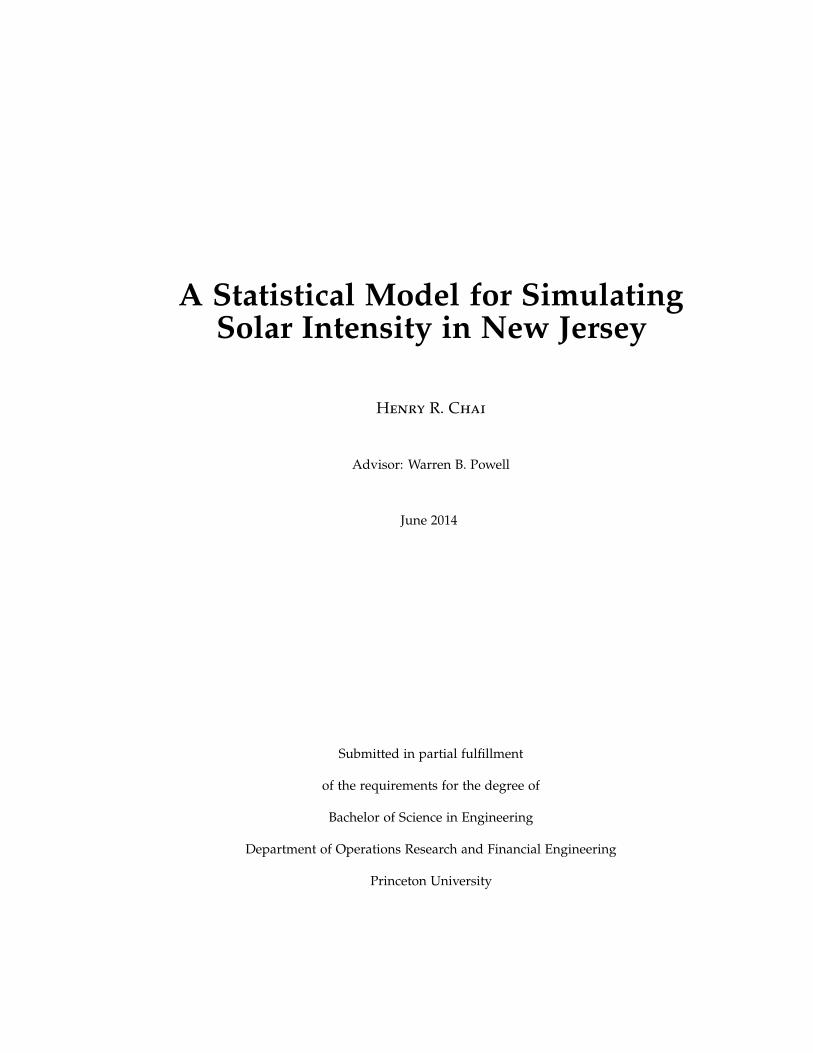
Photovoltaic solar energy infrastructure in the United States has seen a drastic rise in the past
few years: in the three years between the third quarter of 2010 and the third quarter of 2013, the
amount of PV solar energy capacity added in the US grew by 520% (SEIA, 2013). As of 2014, the
PV capacity in the US surpassed 5 GW, putting the US above China in terms of PV capacity and
making it the country with the largest utility-scale PV capacity (Meza, 2014).
Figure 1: US Added PV Capacity from 2010 to 2013
Source: http://www.seia.org/research-resources/solar-industry-data
One interesting aspect of the distribution of PV capacity in the United States is that New
Jersey has the second highest capacity for solar PV energy of all the states, behind only California
(NREL, 2013). This is despite the fact that New Jersey is one of the states with the lowest potential
access to solar PV energy (Lopez et al., 2013). The anomaly that is the high capacity for PV energy
in New Jersey can partially be explained by New Jersey’s renewable portfolio standard (RPS), a
piece of legislation enacted in 1999 and subsequently amended in 2001 which requires that by
1

2020, 20.38% of all electricity generated in New Jersey needs to come from a defined subset of
renewable sources (solar among them) as well as requiring that 4.1% of electricity generated in
the year 2027 comes from solar (DSIRE, 2013). In addition, the RPS established a solar renewable
energy certificates (SREC) market, a market where utilities providers are able to trade certificates
received from generating solar power so that all providers are able to meet their own specific solar
generation quotas.
Figure 2: Estimated Technical Potential for Utility-Scale Photovolatics
Source: http://www.nrel.gov/docs/fy12osti/51946.pdf
Although solar is a renewable source of energy, it does face some problems that make it less
desirable than conventional fossil fuels: solar intensity is difficult to forecast correctly and can vary
quite rapidly, changing from high output levels to low ones in the course of a few minutes. Because
of this volatility, it is difficult for grid operators to depend on solar energy as a reliable way of
meeting electrical demand. This same volatility poses a problem to solar energy providers as well
in that volatility makes it difficult to assess the profitability of a venture. Thus, one necessary step
in the introduction of solar energy into the grid is an effective means of forecasting solar intensity
on a small time scale. The perspective of this work will be that of the utilities provider interested
in selling solar energy into the grid. With that in mind, Section 1.1. will examine the relationship
between PJM Interconnections, a regional trasmission organization that supplies electricity to New
2

Jersey, and PSE&G a major utilities provider in New Jersey. Section 1.2. will explore the possibility
of solar generation in conjunction with electrical storage and potential efficiency gains. Lastly,
Section 1.3. will be an overview of the rest of this thesis.
1.1. PJM and PSE&G
Pennsylvania, New Jersey and Maryland Interconnections (PJM) is the regional transmission
organization (RTO) that coordinates the movement of wholesale electricity in the state of New Jersey.
PJM does not generate any electricity but rather takes electricity generated by utilities providers
and delivers it to demand nodes i.e. buses where electricity is drawn from the interconnection.
PJM operates under an unregulated bidding system where utilities providers submit supply offers
i.e. how much electricity they can provide and the minimum price at which they would be willing
to sell their electricity, both on an hourly basis. Luckily for renewable energy generators, the
operating cost for renewables is zero or negligible so they will always be selected by the RTO to
provide electricity. All the providers are then paid the price that PJM sets in order to guarantee
that they can meet forecasted demand i.e. the minimum price such that the sum of all pledged
generations at or below that price is equal to or greater than the forecasted demand. These prices
are called locational marginal prices or LMPs. Of course, as with any forecasting process, the
demand forecasting is not perfect and often PJM is forced to call upon quick response generators
to meet the gap, which in turn can result in LMP spikes. However, as this work is more concerned
with the perspective of the utilities provider, we will ignore the details concerning how RTOs match
supply and demand, an incredibly complex process.
Public Service Electric and Gas Company (PSE&G) is a major utilities provider in the state of
New Jersey. One of PSE&G’s subsidiaries is PSEG Solar Source, LLC, a major player in the field
of solar generation in New Jersey. On May 29th, 2013, the New Jersey Board of Public Utilities
approved PSE&G’s $446 million plan entitled Solar 4 All (Friedman, 2013). A portion of PSE&G’s
3

Solar 4 All plan includes the construction of 42 MW of solar farms on top of unused land such as
landfills and brownfields; in a densely populated state like New Jersey, if solar generation is going
to play a major role in the electricity portfolio, an efficient use of unwanted land is necessary. The
data for this work is largely provided by PSE&G and consists of solar generation data at the 24
different locations PSE&G is using for their Solar 4 All program.
Figure 3: Example of Solar Farm on Unused Land in NJ
Source: http://pseg.com/family/pseandg/solar4all/index.jsp
As a utilities provider, PSE&G pledges the electricity generated at the power plants owned
by its subsidiaries to PJM Interconnections. This includes the electricity generated at the solar
farms owned by PSEG Solar Source, LLC. In essence, this work is focused on two major problems
facing a utilities provider, such as PSE&G, when considering a push towards increased solar energy
production: firstly, a good forecast model of solar intensity is required to forecast potential power
generation levels and assess the profitability of any solar energy generation projects. Secondly,
current technologies are generally not sufficient to make solar energy projects profitable unless
they are paired with electrical storage so it is necessary to develop an optimal strategy for utilizing
storage in conjunction with solar energy generation.
1.2. Renewable Energy and Storage
The usage of energy storage to deal with the variability of renewable sources of energy is
well documented (Kim & Powell, 2009, Scott & Powell, 2012 and Costa et al. 2008). However, a
lot of these sources deal specifically with the conjunction of wind energy and storage. That being
4

said, solar suffers from many of the same problems that wind does in terms of variability. NREL
suggests that the degree of variability from both sources is similar, although certain aspects such as
sunrise and sunset make solar slightly more predictable; in addition, the variability of both sources
can be reduced if the generation of many plants is aggregated (NREL, March 2013). Thus, the
ability of storage to arbitrage in the PJM market is equally applicable to solar as it is to wind.
Figure 4: Relationship Between Renewables, Storage and the Grid
Source: http://energysystems.princeton.edu/
A more concrete example of arbitrage with a battery can be given using the PJM LMPs:
the average LMP between January 5th, 2013 and July 21st, 2013 was around $44/MW while the
maximum price in that time period was around $693/MW; if one were able to buy low and sell
high, there is clearly the potential to make a great deal of money. Unfortunately, in practice, one
cannot implement so-called offline algorithms, algorithms with perfect knowledge of the future
prices and thus, a more subtle technique will be required to profit from this opportunity. Another
key function of storage when combined with renewables is its ability to compensate for some of the
renewable source’s variability. Because energy suppliers need to make hour-ahead commitments
of the amount of energy they are willing to supply to PJM, storage allows suppliers of renewable
energy to make commitments despite the variability of renewables as the storage will potentially
make up the difference between their commitment and their actual generation if they fall short.
5

This work will make two simplifying assumptions concerning the behavior of batteries: firstly,
the amount of power provided by the renewable energy supplier is negligible relative to the scale
of the market into which it is selling. This implies that the RTO in question, in this case PJM,
will always buy all of the energy pledged by the renewable energy supplier. In addition, this
implies that if the energy provider’s commitment exceeds the amount of energy available from
both solar and storage, they can purchase energy from the grid at the spot price to meet their
commitment. The second assumption concerns the physical properties of the battery. There are
complex physical processes associated with the storage of electricity: stationary lead-acid batteries,
a common existing form of electrical storage, have round trip efficiencies of 70%, which means
that 30% of the electricity put into the battery is lost in transit. In addition, stationary lead-acid
batteries have self-discharge rates of 2% per month and have limited discharge rates (Brunet, 2011).
For this work, we will only consider the capacity limitations and the efficiency losses, as the other
factors, though relevant, are beyond the scope of this work.
1.3. Thesis Overview
This work first describes the relevant models and mathematical tools used here in Section
2. Section 3 describes the datasets used in this work. Section 4 details the utilization of the
mathematical tools and models in the context of a solar energy provider with access to storage
looking to optimize their performance while Section 5 contains the results of the analysis performed
in Section 4. Lastly, Section 6 gives conclusions about the results from Section 5 and possible areas
of future research.
6

2. Models and Methods
This work largely relies on two major concepts, one from the field of statistics and the other
from operations research. The first portion of this work is devoted to constructing a model that
simulates the amount of solar energy, measured in kilowatt hours, that is generated every minute at
each of 24 locations in New Jersey corresponding to 24 locations selected by PSE&G for their Solar 4
All program. This portion relies heavily on autoregressive (integrated) moving-average (AR(I)MA)
time series models. The second part of my thesis will focus on developing an application of the
simulator built in the first part, namely a comparison of the profitability of grid-level storage versus
the profitability of storage cells paired with each individual solar power generation plant. This
portion will utilize the concept of a dynamic program and approximate dynamic programming as
a means of solving dynamic programs.
2.1. ARIMA and ARMA Models
An autoregressive (integrated) moving average model (AR(I)MA) is a time series model
wherein the next element in the series is affected by a finite number of previous values in the series.
More specifically, an ARMA(p,q) model combines an AR (autoregressive) model with p parameters
and an MA (moving average) model with q parameters. The general equation for an ARMA(p,q)
model is:
St = µ +p
∑i=1
φi(St−i − µ) +q
∑j=1
θjεt−j + εt
where St is the amount of solar energy produced during the tth time period, µ is the expected value
of St, {φ1, ..., φp} are the parameters of the AR model, {θ1, ..., θq} are the parameters of the MA
model and ε1, ..., εt is a white noise process with mean 0 and variance σ2ε i.e. WN(0, σ2
ε ). An ARIMA
model differs from an ARMA model in that, under an ARIMA model, the time series is differenced
7
a number times in order to convert it from a non-stationary to a stationary stochastic process,
i.e. one whose joint-probability distribution is constant over time. The differencing operator is
defined as ∆St = St − St−1. Depending on which type of time series model better fits the data,
an ARIMA/ARMA model will be used to simulate z-scores of the errors used as a part of the
simulator.
2.1.1. Literature Review
The original work on ARIMA and ARMA models was done by the statisticians George Box
and Gwilym Jenkins in their work, Time Series Analysis: Forecast and Control (1976). As for the
application of ARIMA and ARMA time series to modeling renewable energy sources, there is
precedent: Huang et al. used ARMA models at UCLA to model solar generation data directly from
historical values (2012). Jin used ARMA/ARIMA time series to model forecast errors, a concept
used here as well, although Jin’s work was related to modeling wind energy generation (2013).
Kavasseri and Seetharaman used fractional ARIMA (f-ARIMA) models, ARIMA models with a
fractionally continuous differencing parameter d ∈ (−0.5, 0.5), to model wind speed; although
fractional ARIMA models display some encouraging characteristics such as slower decay in the
autocorrelation function, making it an attractive option to model time series with long range
correlations (2009); the application of f-ARIMA models in this context is beyond the scope of
this paper. Beyond the precedent for their application, ARIMA/ARMA time series models make
intuitive sense in this context as solar energy generation values are likely to demonstrate some
dependency on previous values; if it is currently cloudy, one would expect it to get either a little
more or a little less cloudy in the next time period, not a sudden jump to maximum sunlight or no
sunlight.
2.1.2. Model Selection
One key component in the utilization of ARIMA/ARMA models is a systematic method of
choosing between different models i.e. determining which set of parameters (p,d,q) results in the
best fitting ARIMA model. In general there are two methods of determining the goodness of fit of
8

a particular model: Akaike information criterion (AIC) and Bayesian information criterion (BIC).
Both of these information criterion try to balance how well a model fits the sample values and how
complex the model is; by balancing these two aspects, these criterion attempt to avoid the selection
of overfitted models i.e. models that fit the noise associated with the underlying data values as
opposed to fitting the signal. The specific formulation for the AIC and BIC values of a given time
series model are:
AIC = 2k− 2ln(L)
BIC = 2ln(k)− 2ln(L)
where k is the number of parameters in the model, L is the estimated model’s maximized likelihood.
An ideal model would have a high maximum likelihood value and as few parameters as possible
so the objective of the fitting process is to minimize either the AIC or BIC value across a range of
possible ARMA/ARIMA models. Another possible criterion for model selection is the AICc, which
is effectively AIC but with a correction that arises to compensate for finite sample sizes:
AICc = AIC +2k(k + 1)n− k− 1
where n is the sample size. Note that as n increases, AICc approaches AIC. Brockwell and Davis rec-
ommend the use of AICc specifically for the purpose of fitting ARMA models to time series (1991).
In addition, the ARMA fitting command in R outputs AICc as the default criterion for time series
fitting so that is what this work utilizes as the basis of choosing an appropriate ARMA/ARIMA
model.
9

2.2 Dynamic Programs and Approximate Dynamic Programming
Dynamic programming, most generally, is the practice of recursively breaking down a large
complex problem into a series of decisions made over multiple time steps. The methodology for
constructing and solving a dynamic program used in this work is taken from Powell’s Approximate
Dynamic Programming, in which he outlines the five components of a dynamic programming
problem: a state variable, decision variables, exogenous information, a transition function and an
objective or contribution function (2010). Recall that the problem that this work is seeking to solve
is the profitability of a single large storage cell versus many smaller storage cells paired with each
individual solar generation plant. Thus, two separate dynamic programs will be run, one for the
scenario involving grid-level storage and another for the plant-level scenario.
2.2.1. State Variable
From Powell’s work, a state variable is the minimally dimensioned function of history that
is both sufficient and necessary to compute the remaining aspects of the dynamic program, the
decision variables, the transition and the objective functions (2010). For this problem the state
variable can be defined as:
St = {R, Rt, pt, ρI , ρO}
where R is the maximum capacity of the battery, Rt is the amount of charge in the battery at
time t, Dt is the demand for electricity at time t, pt is the price of electricity at time t, ρI is the
percentage of energy lost when energy is put into the battery and ρO is the percentage of energy
lost when energy is pulled out of the battery; as percentages, both ρI and ρO are ∈ [0, 1] and, from
our simplifying assumption above, ρIρO = 0.7. Another further simplifying assumption made in
this model is that ρI = ρO and thus ρI = ρO ≈ 0.85. Note that for the plant-level scenario, the
variables R and Rt are vectors where each plant’s storage cell will have a value.
10

2.2.2. Decision Variables
The decision variables are the values that the dynamic program is trying to optimize over. For
this problem, the decision variables can be mathematically expressed as:
Dt = {Fτ+1, EBGt , ESB
t , ESGt }
where Fτ+1 is the commitment made by the utilities provider for the next time period, G represents
the grid, B represents the battery, S represents the solar power and EAA′t is the quantity of
electricity transfered from location A to location A’ during the tth time period. Both ESBt and ESG
t
are constrained to be non-negative while EBGt can be either positive or negative, with negative
values indicating a transfer of electricity from the grid to the battery i.e. buying electricity. Note
that PJM requires utility providers to make hour ahead commitments about the amount of energy
they are able to provide in the next hour so the quantity Fτ+1 is indexed by a different value, τ not
t, because the time steps for the other variables in this problem are in five minute increments.
2.2.3. Model Constraints
The two main constraints that the decision variables are subject to can be called the capacity
constraint and the commitment constraint: the capacity constraint dictates that the battery cannot
hold more than its capacity, R, at any time step while the commitment constraint says that the total
electricity sold to the grid in any hour must be greater than or equal to the commitment made at
the beginning of that hour (recall that one of the simplifying assumptions stated above is that due
to the small size of the renewable provider relative to the market, all excess generation can be sold
at the spot price). These constraints can be modeled mathematically as the following equations:
R ≥ Rt + ρI ESBt − EBG
t ∀ t
Fτ ≤12τ
∑i=12τ−11
(ESGi + ρOEBG
i ) ∀ τ
11

2.2.4. Exogenous Information
The exogenous information in a dynamic program contains the values that arrive after each
time period and affect the state of the problem. For this problem, the exogenous information can
be expressed as:
Wt = {St−1, pt}
where pt is the change in the price of electricity from the t− 1th time period to the tth time period
and St is the amount of solar energy generated in the tth time period.
2.2.5. Transition and Objective Function
The transition function is a set of functions that maps the individual elements in the state
variable at time t to their respective elements in the state variable at time t+1. Using this notation,
the transition function for this problem can be expressed as the following series of equations:
Rt+1 = Rt + ρI ESBt + EGB
t
pt+1 = pt + pt+1
Lastly, the objective function for this problem is to maximize revenue across a finite time horizon
of T time periods and can be expressed as such:
maxDt
T
∑t=1
pt(ρOEBGt + ESG
t )−T/12
∑τ=1
pt
(Fτ −
12(τ−1)+12
∑t=12(τ−1)+1
St
)
2.2.6. Approximate Dynamic Programming
Due to the complexity of most dynamic programs, it is often necessary to use additional tools
to simplify them and come up with an approximation of the optimal solution. The practice of
doing so is called approximate dynamic programming. One commonly used tool for this purpose
is a policy function approximation (PFA), which Powell describes as a function that maps states to
12

decisions without any optimization or forecast of future exogenous information (2010). Generally,
PFAs come with tunable parameters which can improve the performance of the policy. The PFA
that this work uses can be described as follows: commitments are made based on applying the
simulator developed in the first part and simulating future solar generation values. As for the
decisions made at the five minute increments, if the LMP is above a threshold Pss, then the policy
is to sell all solar energy generated and all electricity in the battery. If the LMP is less than Pss
but greater than Ps, then the policy is to sell all solar energy generated. If the LMP is less than Ps
and greater than Pb, then store electricity generated by solar until the battery is full and sell the
rest to the grid. Lastly, if the LMP is below Pb, then the policy stores all generated solar energy
into the battery and if the battery is still not full, buy electricity from the grid until it is. Because
commitments are made at the hour level, if at the time period immediately proceeding the end
of an hour the total electricity sold to the grid in that hour is less than the commitment, then
electricity is bought from the grid at the current spot price to make up the difference.
In the PFA described above, the tunable parameters are Pss, Ps and Pb, which can be adjusted
to improve the policy’s performance. This method is called approximate dynamic programming
(ADP) as it attempts to approximate the solution to the dynamic program as opposed to running
an optimization program over the problem itself because in general, dynamic programs are difficult
to optimize directly. In its most general form, ADP implements policy improvement in an outer
loop while running policy evaluation for a fixed policy in an inner loop over the fixed time horizon,
selecting the policy at the end that performed the best.
13

3. Sources of Data
The major data sets used in this work are historical solar energy generation values and PJM
LMPs. The solar generation data is provided by PSE&G while the LMP data is provided by PJM.
The data sets are described in greater detail in Sections 3.1. and 3.2.
3.1. Solar Energy Generation Data
The main source of solar generation data for this project is a data set provided by PSE&G, a
major utilities provider in New Jersey with numerous solar power plants operating around the
state. The data set consists of solar energy generation values for 24 different solar power plants
across the state. The values in the data set are at the one minute level and in units of kilowatt-hours.
The data set spans one year, beginning on September 1st, 2012 and going to October 31st, 2013. The
data set described above will be used in the construction of the statistical solar energy simulator.
There were some issues with the raw data: certain days would have their entire output summed
up in a single entry at the beginning of the day or certain days would have a constant, non-zero
output throughout the entire day. These issues were taken care of manually with some amount
of preprocessing; days that were marked as outliers were replaced with the values from the day
before.
Another consideration necessary to make when utilizing this dataset is the units of the other
dataset; the next data set is in five minute increments with units of price per MW, which means
that it is necessary to first aggregate the data into increments of five minutes by summing up all
the generation values in each five minute interval. Lastly, the generation values are converted from
kWh to MW by multiplying by a factor of 0.012.
14

3.2. PJM Local Marginal Price Data
This thesis also relies on a data set provided by the Pennsylvania, New Jersey, Maryland (PJM)
Interconnection LLC, which contains the local marginal prices (LMPs) for electricity in the PJM
electricity market, including the PSE&G zone within the PJM region. This data set contains all
of the LMPs in New Jersey at five minute intervals, with units of USD per MW, between January
1st, 2013 and July 22nd, 2013. This dataset will be used in the dynamic programming portion of
this work as the grid price of electricity portion of the exogenous information variable. As noted
above, the data in this dataset are incredibly volatile; although the average LMP during the time
period above is around $44/MW, the maximum of the dataset is around $693/MW. The PJM data
set also contains data on the demand for electricity at five minute intervals for each distribution
node i.e. the load, another statistic which could be used to refine or contextualize the dynamic
programs used to model electrical storage. However, it is assumed by this work that the demand
for electricity far exceeds the amount of energy supplied by solar generation and therefore, the
demand is irrelevant to the dynamic programs’ construction.
15
4. Solar Generation Simulator and Dynamic Program
As initially noted, the first goal of this work is to construct a solar energy generation simulator
using historical data. The second goal is to utilize this simulator to determine whether grid-level
storage i.e. a single, large battery which stores energy relative to the production of all 24 solar
generation plants is more profitable than storage cells paired with the individual generation plants.
Thus, this section will first begin by describing the methodology of constructing the simulator and
then describing the set up of the dynamic program.
4.1. Solar Generation Simulator Methodology
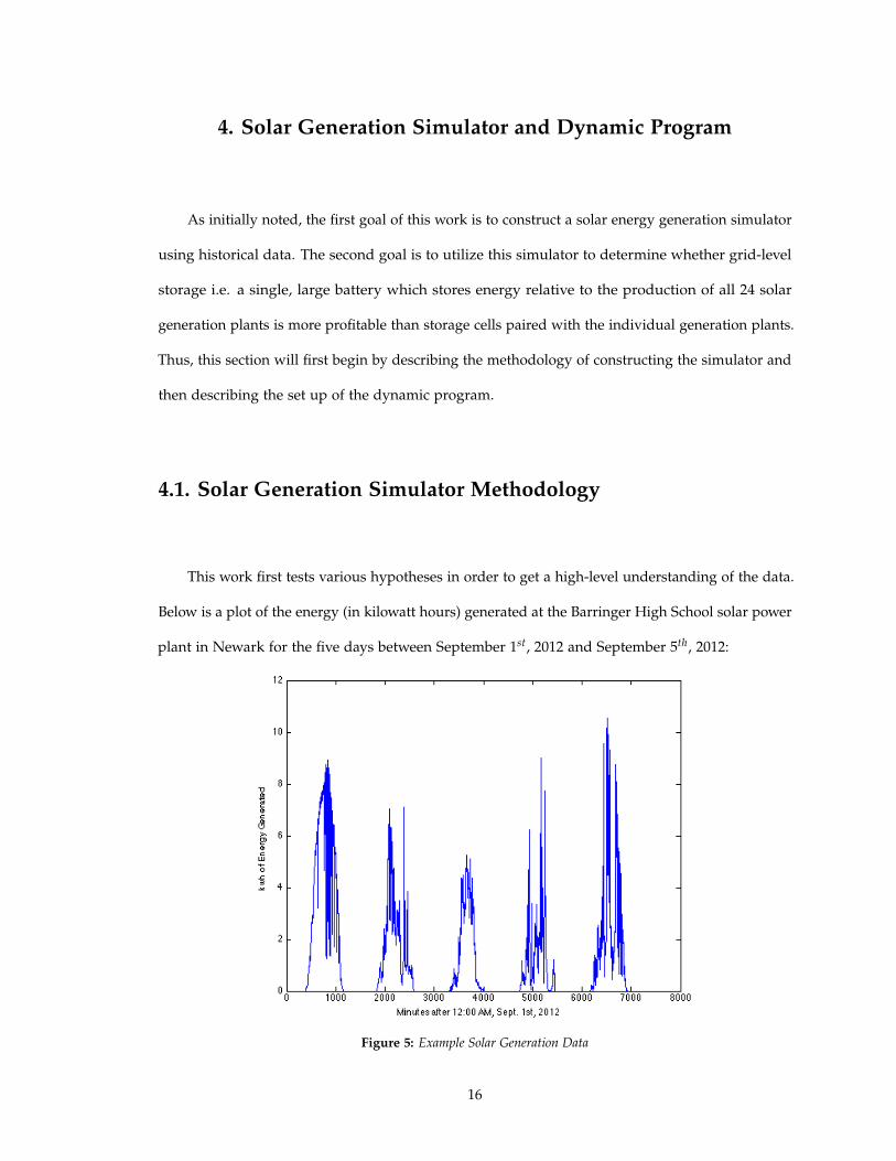
This work first tests various hypotheses in order to get a high-level understanding of the data.
Below is a plot of the energy (in kilowatt hours) generated at the Barringer High School solar power
plant in Newark for the five days between September 1st, 2012 and September 5th, 2012:
Figure 5: Example Solar Generation Data
16
The figure shows some interesting trends: there is of course a predictable trend of increasing
generation up to the point during the day when the solar radiation reaches peak intensity at which
point we see a decrease in the energy generation. However, there is a great deal of noise, both
within a given day and across multiple days. It is reasonable to conclude that the large decreases in
energy generation during a given day occur due to cloud cover, as cloud cover decreases the solar
intensity, which in turn limits the amount of energy that can be produced via photovoltaic cells.
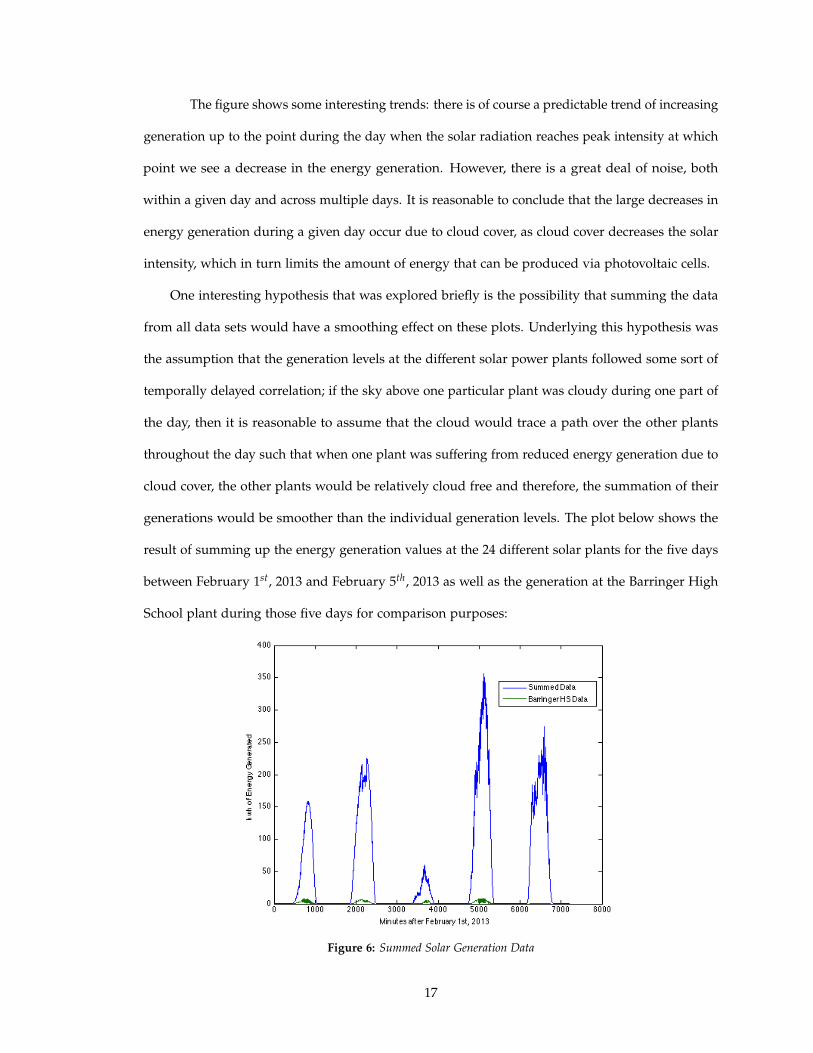
One interesting hypothesis that was explored briefly is the possibility that summing the data
from all data sets would have a smoothing effect on these plots. Underlying this hypothesis was
the assumption that the generation levels at the different solar power plants followed some sort of
temporally delayed correlation; if the sky above one particular plant was cloudy during one part of
the day, then it is reasonable to assume that the cloud would trace a path over the other plants
throughout the day such that when one plant was suffering from reduced energy generation due to
cloud cover, the other plants would be relatively cloud free and therefore, the summation of their
generations would be smoother than the individual generation levels. The plot below shows the
result of summing up the energy generation values at the 24 different solar plants for the five days
between February 1st, 2013 and February 5th, 2013 as well as the generation at the Barringer High
School plant during those five days for comparison purposes:
Figure 6: Summed Solar Generation Data
17
As the figure shows, although summing the data does make the generation values within
a given day smoother, there is still a great deal of variance across the days. The smoother days
suggests that there might be some temporally delayed correlation between energy generation at
different locations. In addition, significant variance across multiple days suggests a great deal
of correlation on the scale of days; when generation is low for an entire day at a given location,
it seems that generation is low at all the locations for that day i.e. if it remains cloudy over one
location for an entire day, this implies that the cloud cover is significant enough to span the entire
area that contains the 24 different plant locations and diminish generation levels at every location
for that day, regardless of how the cloud cover might shift during the day. The concept of summing
the data to decrease variability was mentioned above and will be returned to when discussing the
benefits of grid-level versus individual plant level storage.
4.2. Solar Energy Model
The solar energy generation simulator will consist of two components: a baseline estimate
of the solar energy and a statistical error generator. A model similar to this was used by Jin to
simulate wind energy (2013). For the baseline, this work uses a model for the amount of solar
energy that hits each location on a sunny, cloudless day. Specifically this baseline model will be
the maximum energy generated at each minute over the previous 21-day period as given by the
dataset itself. Then the offset error for each measurement can be modeled as a value between 0
and 1 that represents the fraction of the baseline model that is the simulated value. These errors
are the sample values that will be fit to an ARIMA or ARMA model. However, again building off
of the work done by Jin in the field of wind energy simulation, instead of directly simulating the
error values themselves, the quality of the simulation can be improved by constructing cumulative
distribution functions (CDFs) for the errors, evaluating the z-scores of each sample offset error,
fitting the ARIMA model to these z-scores and then converting the simulated z-scores into offset
18

errors by using the CDF constructed before. This method more accurately captures the behavior
of the errors because it is effectively sampling from the distribution of known errors as opposed
to guessing at the error’s distribution. Lastly, the simulated errors are multiplied by the 21-day
maximums to create simulated solar energy generation values.
4.2.1. Baseline Model Construction
After experimenting with various physical models of solar energy and intensity with various
considerations such as latitude, time of day and date, it was concluded that the best approach was
to use the dataset itself to determine a potential baseline model for the maximum solar intensity.
The approach taken by this work is as follows: for any given day and power plant, look three
weeks into the past and find the maximum value for energy generation at that power plant for
each minute. A plot of the maximum values, calculated using the approach described above, at
the Barringer High School solar plant over the 21 days preceding September 22nd, 2012 is shown
below, along with the actual energy generation levels on September 22nd, 2012 at the Barringer
High School solar plant for comparison purposes:
Figure 7: Maximum Solar Generation Data
19
The search for maximum values was limited to three weeks behind to avoid running into
severe seasonal variations; the idea behind finding a baseline model was that it ought to resemble
the maximum possible sunlight that hits a given location based off of geographic and seasonal
factors. The assumption underlying this approach is that there should be at least one sunny,
cloudless day in every three week period. Thus, using the maximum value for each individual
plant across a short horizon should provide a reasonable estimate of our desired baseline model
for the maximum potential generation.
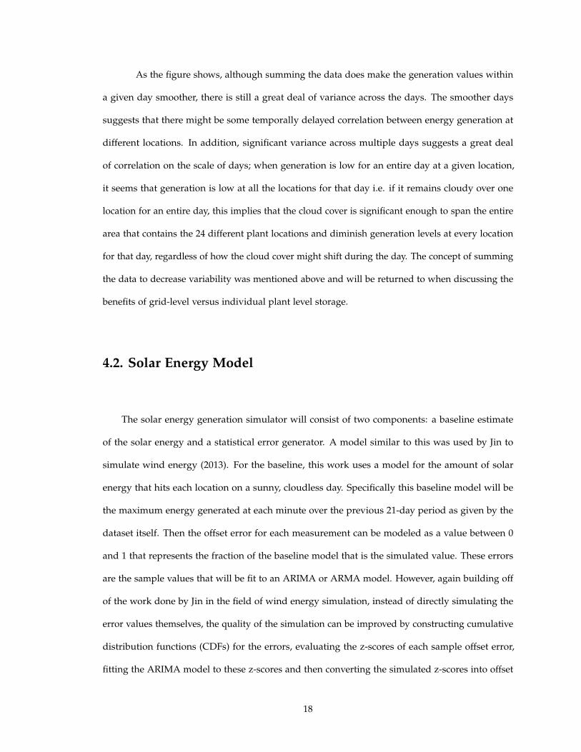
4.2.2. Sample Offset Calculation
After the rolling maximums are calculated for each day (beyond the 21st day because for the
first 21 days, there is insufficient historical data to calculate rolling maximums), the next step
was to calculate the offset errors, evaluated for each sample generation value by dividing the
actual generation at the given minute by the maximum generation value for that minute across the
previous 21 days. The figure below shows the offset errors for the five days between September
22nd, 2012 and September 26th, 2012 at the Barringer High School solar energy generation plant:
Figure 8: Calculated Offset Errors
20
In theory the offset errors should be between one and zero, but as the figure above shows,
there are instances where the the offsets spike above one. This is because the calculated maximums
exclude the given day so on certain days, the generation values spike above the maximum genera-
tion values in the previous 21 days. In the figure above, it is interesting to note that some of the
days have offsets that resemble the actual generation values; this makes sense because on sunny
days, the ratio of the actual and maximum generations should hover around one, with the only
potential significant differences occurring around the timing of sunrise and sunset, which are seen
in the figure as the ramps up and down visible in some of the days.
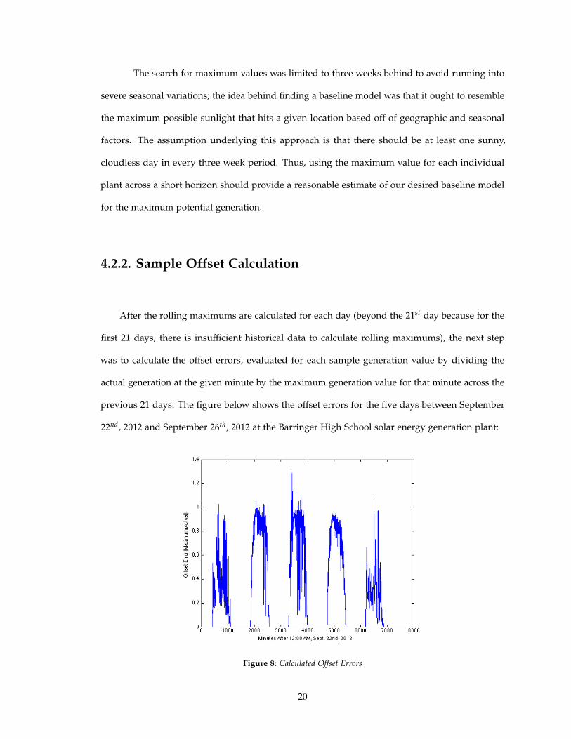
4.2.3. CDF Construction and Z-Score Calculation
The next step in constructing the simulator was to calculate the cumulative distribution
functions (CDFs) for each set of 21 days. The figure below shows an example of a constructed CDF.
Specifically it is the CDF constructed using the first 21 days, between September 22nd and October
12th, worth of offsets calculated at the Barringer High School solar plant:
Figure 9: Cumulative Distribution Function of Offset Errors
21
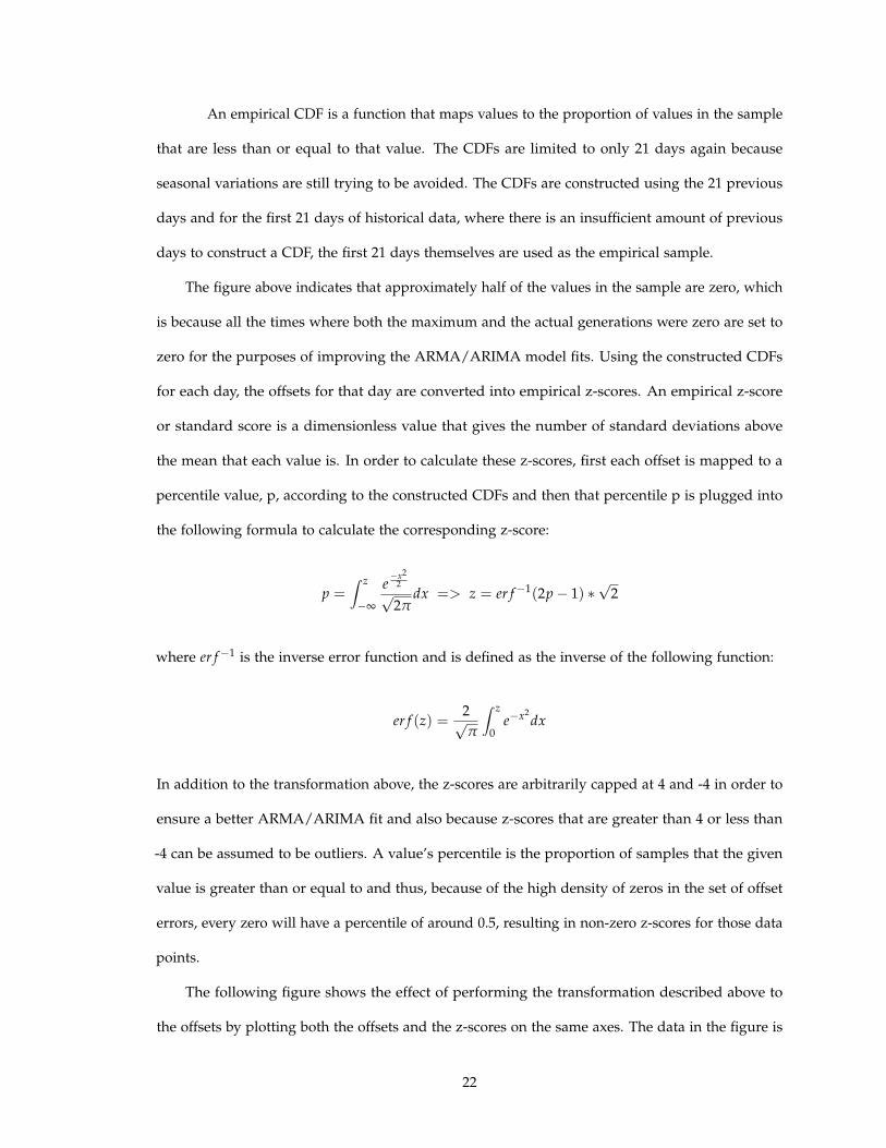
An empirical CDF is a function that maps values to the proportion of values in the sample
that are less than or equal to that value. The CDFs are limited to only 21 days again because
seasonal variations are still trying to be avoided. The CDFs are constructed using the 21 previous
days and for the first 21 days of historical data, where there is an insufficient amount of previous
days to construct a CDF, the first 21 days themselves are used as the empirical sample.
The figure above indicates that approximately half of the values in the sample are zero, which
is because all the times where both the maximum and the actual generations were zero are set to
zero for the purposes of improving the ARMA/ARIMA model fits. Using the constructed CDFs
for each day, the offsets for that day are converted into empirical z-scores. An empirical z-score
or standard score is a dimensionless value that gives the number of standard deviations above
the mean that each value is. In order to calculate these z-scores, first each offset is mapped to a
percentile value, p, according to the constructed CDFs and then that percentile p is plugged into
the following formula to calculate the corresponding z-score:
p =∫ z
−∞
e−x2
2√
2πdx => z = er f−1(2p− 1) ∗
√2
where er f−1 is the inverse error function and is defined as the inverse of the following function:
er f (z) =2√π
∫ z
0e−x2
dx
In addition to the transformation above, the z-scores are arbitrarily capped at 4 and -4 in order to
ensure a better ARMA/ARIMA fit and also because z-scores that are greater than 4 or less than
-4 can be assumed to be outliers. A value’s percentile is the proportion of samples that the given
value is greater than or equal to and thus, because of the high density of zeros in the set of offset
errors, every zero will have a percentile of around 0.5, resulting in non-zero z-scores for those data
points.
The following figure shows the effect of performing the transformation described above to
the offsets by plotting both the offsets and the z-scores on the same axes. The data in the figure is
22
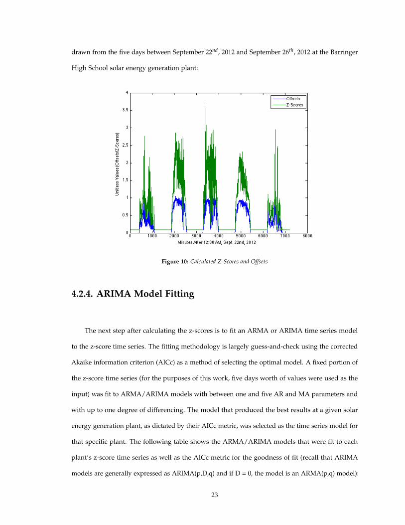
drawn from the five days between September 22nd, 2012 and September 26th, 2012 at the Barringer
High School solar energy generation plant:
Figure 10: Calculated Z-Scores and Offsets
4.2.4. ARIMA Model Fitting
The next step after calculating the z-scores is to fit an ARMA or ARIMA time series model
to the z-score time series. The fitting methodology is largely guess-and-check using the corrected
Akaike information criterion (AICc) as a method of selecting the optimal model. A fixed portion of
the z-score time series (for the purposes of this work, five days worth of values were used as the
input) was fit to ARMA/ARIMA models with between one and five AR and MA parameters and
with up to one degree of differencing. The model that produced the best results at a given solar
energy generation plant, as dictated by their AICc metric, was selected as the time series model for
that specific plant. The following table shows the ARMA/ARIMA models that were fit to each
plant’s z-score time series as well as the AICc metric for the goodness of fit (recall that ARIMA
models are generally expressed as ARIMA(p,D,q) and if D = 0, the model is an ARMA(p,q) model):
23
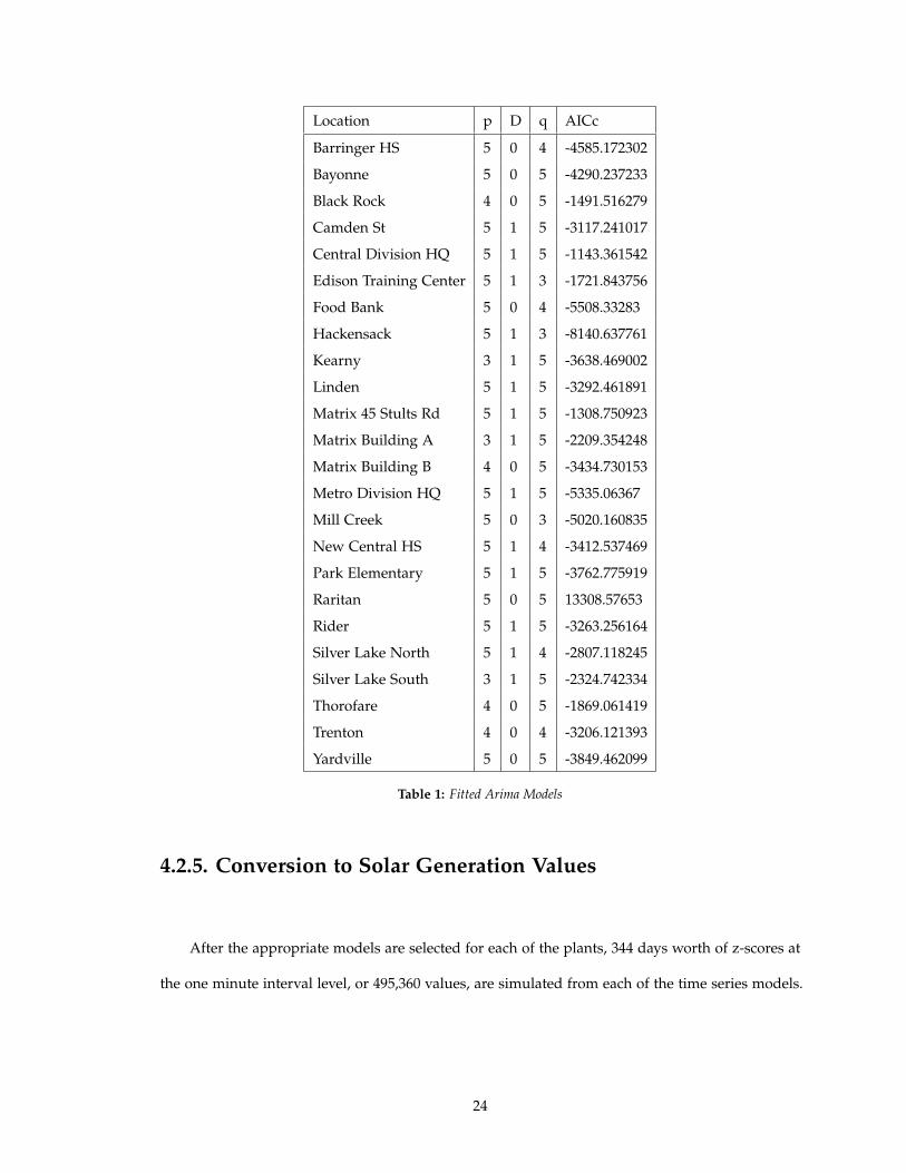
Location p D q AICc
Barringer HS 5 0 4 -4585.172302
Bayonne 5 0 5 -4290.237233
Black Rock 4 0 5 -1491.516279
Camden St 5 1 5 -3117.241017
Central Division HQ 5 1 5 -1143.361542
Edison Training Center 5 1 3 -1721.843756
Food Bank 5 0 4 -5508.33283
Hackensack 5 1 3 -8140.637761
Kearny 3 1 5 -3638.469002
Linden 5 1 5 -3292.461891
Matrix 45 Stults Rd 5 1 5 -1308.750923
Matrix Building A 3 1 5 -2209.354248
Matrix Building B 4 0 5 -3434.730153
Metro Division HQ 5 1 5 -5335.06367
Mill Creek 5 0 3 -5020.160835
New Central HS 5 1 4 -3412.537469
Park Elementary 5 1 5 -3762.775919
Raritan 5 0 5 13308.57653
Rider 5 1 5 -3263.256164
Silver Lake North 5 1 4 -2807.118245
Silver Lake South 3 1 5 -2324.742334
Thorofare 4 0 5 -1869.061419
Trenton 4 0 4 -3206.121393
Yardville 5 0 5 -3849.462099
Table 1: Fitted Arima Models
4.2.5. Conversion to Solar Generation Values
After the appropriate models are selected for each of the plants, 344 days worth of z-scores at
the one minute interval level, or 495,360 values, are simulated from each of the time series models.
24

These simulated values are then put into the inverse of the formula used to calculate the z-scores:
∫ z
−∞
e−x2
2√
2πdx = p
The percentiles calculated in this manner are guaranteed strictly between 0 and 1 because:
e−x2
2√
2π> 0 ∀ x and 0 ≤
∫ z
−∞
e−x2
2√
2πdx ≤
∫ z
−∞
e−x2
2√
2πdx = 1 ∀ −∞ ≤ z ≤ ∞
The percentiles output for each of the simulated z-scores are then converted back into offset
errors using the perviously constructed CDFs for each of the generation plants. This is done by
calculating the inverse cumulative distribution function which takes as input a number between
0 and 1 and returns the smallest value from the original sample that is higher than the input
proportion of values in the original sample. Lastly, the errors are multiplied by the 21-day
maximums calculated in the first step to create simulated solar energy generation values.
4.3. The Solar Energy and Storage Dynamic Program
Moving on to the second portion of this work, the question being answered is whether a single,
large battery which stores and releases energy in conjunction with the total output of the 24 solar
generation plants associated with PSE&G’s Solar 4 All program is a more profitable venture than
an individual, smaller battery with each of the 24 solar generation plants that stores and releases
energy based off of its associated plant’s generation. The initial hypothesis of this work is that the
scenario involving individual batteries will be more profitable because the flexibility associated with
having many batteries operating under independent policies ought to be a sufficiently beneficial
factor to compensate for the larger battery size of the grid-level storage scenario.
The decisions to be made are characterized by the decision variables described in Section 2.2.2.
Thus, the first step to defining this dynamic program is determining the number of time steps that
define the problem; the limiting factor here, in terms of data availability, is the amount of pricing
25

data. As mentioned in Section 3, the pricing data is in LMPs at five minute intervals between
January 1st, 2013 and July 22nd, 2013 meaning that there are 57000 data points.
After determining the number of time steps in the problem, construction of the dynamic
program continues with the simulation of two separate sets of solar generation values of 285000
solar generation values. Note that the number of solar generation values is a factor of five greater
than the number of LMPs available because the solar generation values are simulated at the one
minute interval. Two sets are generated as one of the sets will be the set from which the hour-ahead
commitments are made while the other set will be treated as the actual generation values and used
as a portion of the exogenous variable in the dynamic program. Note that a set of solar generation
values entails independent runs of each of the 24 solar generation plant’s simulators.
At this stage, it is important to note that there are two different dynamic programs being
constructed by this work, one for the grid-level storage cell and another for the individual plant
storage cells. The size of the grid-level battery is defined as twice the sum of each solar generation
plant’s maximum observed generation at the five minute level from the dataset while each of the
individual batteries has a size equal to the maximum observed generation at the five minute level
of its associated solar generation plant. In terms of the values from the data set, this means that
the grid-level battery will have a storage capacity of 5.1652 MWh while the total capacity of all
the individual, plant-level batteries is 2.5826 MWh. These values are well within the realm of an
operational possibility: the DOE database of energy storage project lists multiple examples of
operating storage facilities, utilizing chemical batteries, with capacities on this order of magnitude.
These include the Laurel Mountain storage facility located in Elkins, West Virginia that utilizes
a lithium ion battery with a 8MWh capacity, the Battery Energy Storage System (BESS) facility
in Fairbanks, Alaska that uses a Nickel Cadmium battery with a capacity of 6.25MWh and the
Kahaewa Wind Power Project, located in Maalaea, Hawaii that uses an advanced lead acid battery
with a capacity of 7.5MWh (SNL, 2012).
The battery size here is seemingly arbitrary but all that is necessary for the purpose of
comparison is that the size of the battery used in the grid-level scenario be larger than the sum of
26

the sizes of the individual batteries; if the size is equal to the sum of the sizes of the individual
battery, then the question of which venture is more profitable is trivial as the set of all policies that
could be implemented using the single larger battery is contained in the set of all policies that
could be implemented using the smaller, individual batteries and therefore, the plant-level scenario
is guaranteed to be at least as profitable as the grid-level scenario. One important underlying
assumption of this model is that the cost of electrical storage is linear in the capacity of the battery.
This assumption is validated by Brunet as he estimates the cost of stationary lead-acid batteries as
$300 per kWh of capacity (2011). The linearity of costs relative to capacity is justified because in
practice, storage on this scale is just a collection of smaller batteries. This assumption is important
in that it allows us to calculate the profit as opposed to just the revenue of the policies.
27
5. Results and Discussion
This section will discuss the results of the both the simulator and the dynamic program.
Specifically, it will first examine the results of the simulator and suggest one manner of more
rigorously assessing the quality of the simulators output. Next, this section will examine the results
of the dynamic program, comparing the profitability of grid-level storage versus plant-level storage
cells. In addition, the optimal policy for operating a storage cell in conjunction with solar energy
generation will be elaborated in this section i.e. the optimal policies arrived at given the PFA
described in Section 2.2.5.
5.1. Solar Generation Simulator Results
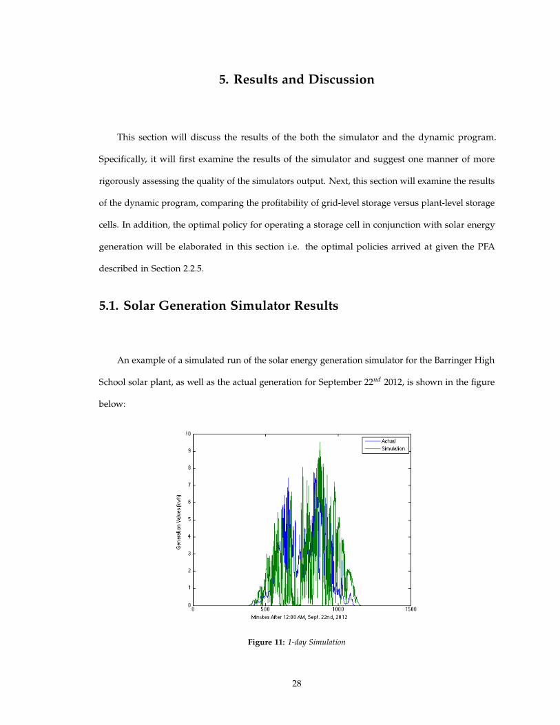
An example of a simulated run of the solar energy generation simulator for the Barringer High
School solar plant, as well as the actual generation for September 22nd 2012, is shown in the figure
below:
Figure 11: 1-day Simulation
28
As the figure above shows, the behavior displayed by the simulator is very similar to the
actual generation at the Barringer High School plant. The overall shape is similar in that there
is a clear sunrise, peak and sunset; however, there are some random spikes downward in the
simulation which are similar to the downward spikes in generation visible in the actual time series,
an encouraging qualitative observation.
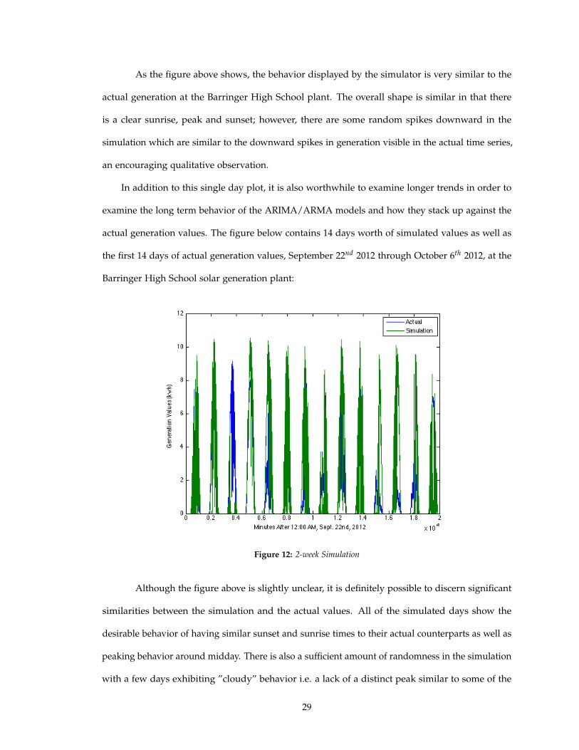
In addition to this single day plot, it is also worthwhile to examine longer trends in order to
examine the long term behavior of the ARIMA/ARMA models and how they stack up against the
actual generation values. The figure below contains 14 days worth of simulated values as well as
the first 14 days of actual generation values, September 22nd 2012 through October 6th 2012, at the
Barringer High School solar generation plant:
Figure 12: 2-week Simulation
Although the figure above is slightly unclear, it is definitely possible to discern significant
similarities between the simulation and the actual values. All of the simulated days show the
desirable behavior of having similar sunset and sunrise times to their actual counterparts as well as
peaking behavior around midday. There is also a sufficient amount of randomness in the simulation
with a few days exhibiting ”cloudy” behavior i.e. a lack of a distinct peak similar to some of the
29
generation values on actual cloudy days. However, in general, the simulated values are slightly
higher than the actual values, which follows because the simulated values are based off of 21-day
maximums.
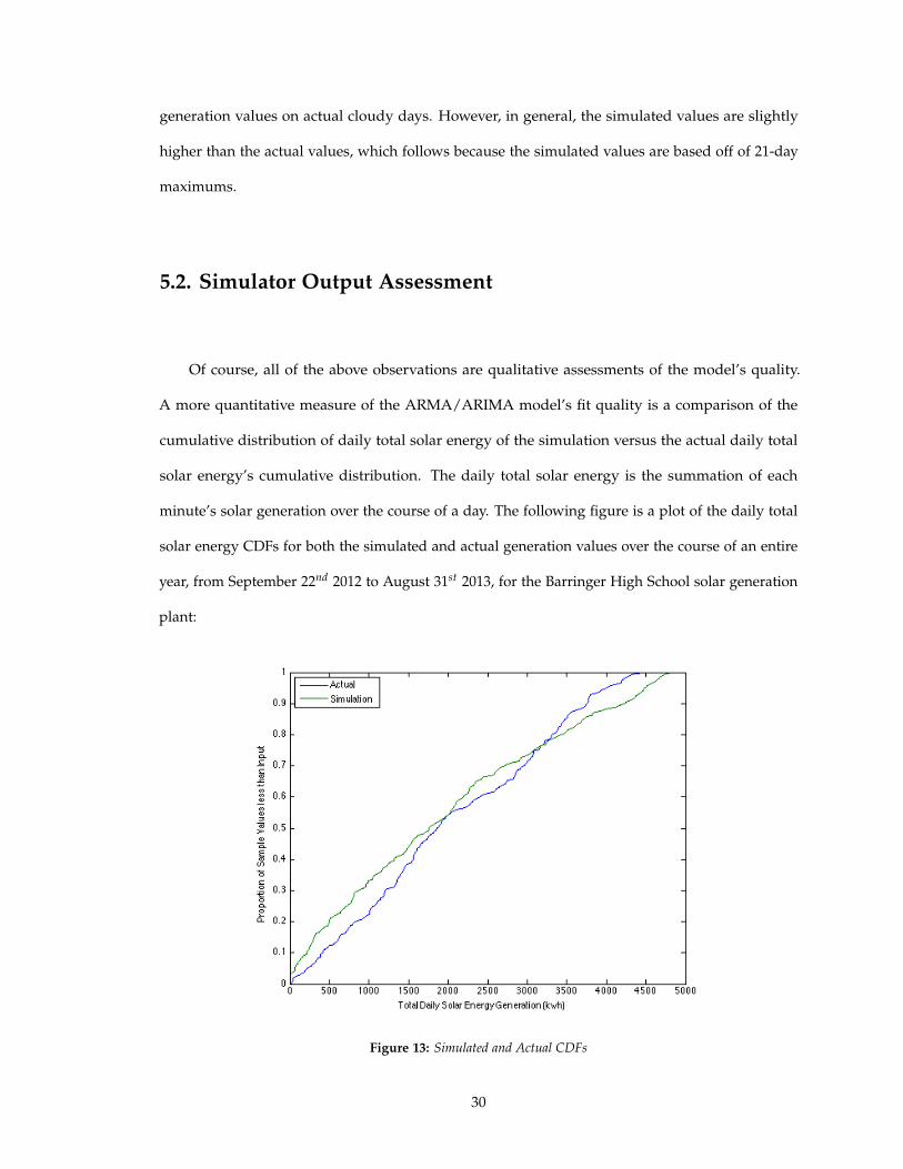
5.2. Simulator Output Assessment
Of course, all of the above observations are qualitative assessments of the model’s quality.
A more quantitative measure of the ARMA/ARIMA model’s fit quality is a comparison of the
cumulative distribution of daily total solar energy of the simulation versus the actual daily total
solar energy’s cumulative distribution. The daily total solar energy is the summation of each
minute’s solar generation over the course of a day. The following figure is a plot of the daily total
solar energy CDFs for both the simulated and actual generation values over the course of an entire
year, from September 22nd 2012 to August 31st 2013, for the Barringer High School solar generation
plant:
Figure 13: Simulated and Actual CDFs
30
The daily total solar energy is a relevant metric of comparison because measuring the
similarity between the forecast and the actual values at the smaller scale of minutes is both difficult
and can be thought of as measuring the overfitting in the model, a metric that is not relevant when
determining the model’s overall quality of fit. As can be seen from the figure above, although the
CDFs do not line up perfectly, they are relatively similar. Qualitatively, the only major difference
seems to be that the slope of the simulation’s CDF is smaller than the actual CDF, which indicates
that the simulation had a higher occurrence of both lower and higher total daily solar generation
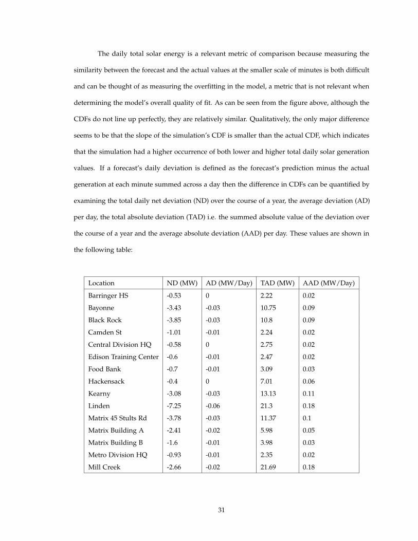
values. If a forecast’s daily deviation is defined as the forecast’s prediction minus the actual
generation at each minute summed across a day then the difference in CDFs can be quantified by
examining the total daily net deviation (ND) over the course of a year, the average deviation (AD)
per day, the total absolute deviation (TAD) i.e. the summed absolute value of the deviation over
the course of a year and the average absolute deviation (AAD) per day. These values are shown in
the following table:
Location ND (MW) AD (MW/Day) TAD (MW) AAD (MW/Day)
Barringer HS -0.53 0 2.22 0.02
Bayonne -3.43 -0.03 10.75 0.09
Black Rock -3.85 -0.03 10.8 0.09
Camden St -1.01 -0.01 2.24 0.02
Central Division HQ -0.58 0 2.75 0.02
Edison Training Center -0.6 -0.01 2.47 0.02
Food Bank -0.7 -0.01 3.09 0.03
Hackensack -0.4 0 7.01 0.06
Kearny -3.08 -0.03 13.13 0.11
Linden -7.25 -0.06 21.3 0.18
Matrix 45 Stults Rd -3.78 -0.03 11.37 0.1
Matrix Building A -2.41 -0.02 5.98 0.05
Matrix Building B -1.6 -0.01 3.98 0.03
Metro Division HQ -0.93 -0.01 2.35 0.02
Mill Creek -2.66 -0.02 21.69 0.18
31
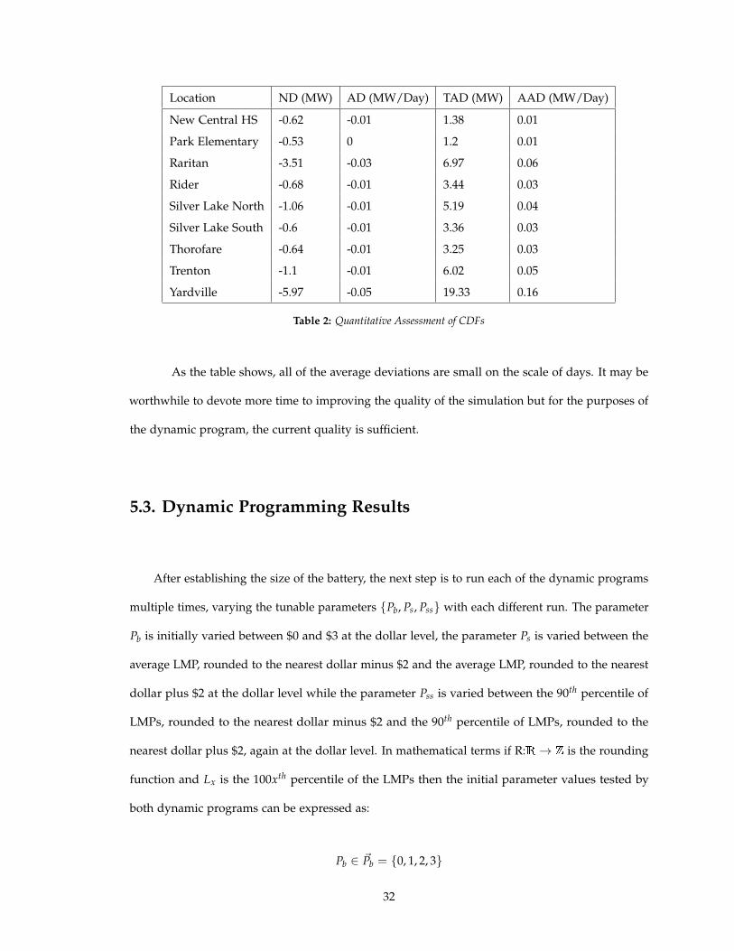
Location ND (MW) AD (MW/Day) TAD (MW) AAD (MW/Day)
New Central HS -0.62 -0.01 1.38 0.01
Park Elementary -0.53 0 1.2 0.01
Raritan -3.51 -0.03 6.97 0.06
Rider -0.68 -0.01 3.44 0.03
Silver Lake North -1.06 -0.01 5.19 0.04
Silver Lake South -0.6 -0.01 3.36 0.03
Thorofare -0.64 -0.01 3.25 0.03
Trenton -1.1 -0.01 6.02 0.05
Yardville -5.97 -0.05 19.33 0.16
Table 2: Quantitative Assessment of CDFs
As the table shows, all of the average deviations are small on the scale of days. It may be
worthwhile to devote more time to improving the quality of the simulation but for the purposes of
the dynamic program, the current quality is sufficient.
5.3. Dynamic Programming Results
After establishing the size of the battery, the next step is to run each of the dynamic programs
multiple times, varying the tunable parameters {Pb, Ps, Pss} with each different run. The parameter
Pb is initially varied between $0 and $3 at the dollar level, the parameter Ps is varied between the
average LMP, rounded to the nearest dollar minus $2 and the average LMP, rounded to the nearest
dollar plus $2 at the dollar level while the parameter Pss is varied between the 90th percentile of
LMPs, rounded to the nearest dollar minus $2 and the 90th percentile of LMPs, rounded to the
nearest dollar plus $2, again at the dollar level. In mathematical terms if R:R→ Z is the rounding
function and Lx is the 100xth percentile of the LMPs then the initial parameter values tested by
both dynamic programs can be expressed as:
Pb ∈ ~Pb = {0, 1, 2, 3}
32

Ps ∈ ~Ps = {R(L0.5)− 2, R(L0.5)− 1, R(L0.5), R(L0.5) + 1, R(L0.5) + 2}
Pss ∈ ~Pss{R(L0.9)− 2, R(L0.9)− 1, R(L0.9), R(L0.9) + 1, R(L0.9) + 2}
These choices of initial parameter settings are justified qualitatively in that one would reason-
ably expect the optimal parameter values to be around the ones chosen here. In order to maximize
profit, a battery operator should attempt the proverbial ”buy low and sell high” strategy: clearly if
the current LMP is below zero, then electricity should be bought as it pays to do so, but it may
be optimal to buy electricity at LMPs slightly higher than zero. Likewise, the battery operator
ought to wait until the price is sufficiently high before selling off stored electricity; in this instance,
sufficiently high is defined in terms of the historical data i.e. around the 90th percentile. Each set
of parameter values is used 10 times in each dynamic program i.e. with 10 different simulated
solar generation values and the profits are averaged together. In addition, a run of the model
without storage is included in order to give a baseline to which results can be compared. The
results of running both dynamic program over these initial policies are depicted both graphically
and numerically below (note that the units of the values in the table are USD):
Baseline Model Summed Generation Individual Generations
Maximum Profit 5415900 4876500 6988900
Table 3: Maximized Profits under the two Scenarios and the Baseline (Initial)
33
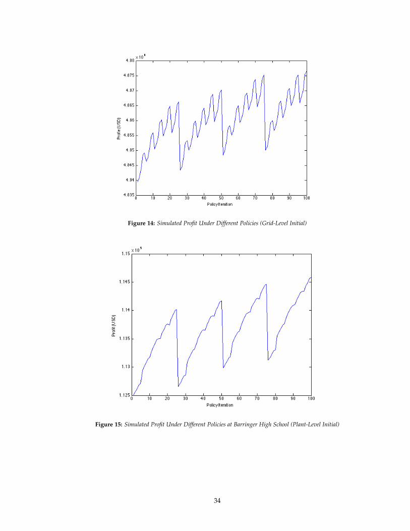
Figure 14: Simulated Profit Under Different Policies (Grid-Level Initial)
Figure 15: Simulated Profit Under Different Policies at Barringer High School (Plant-Level Initial)
34
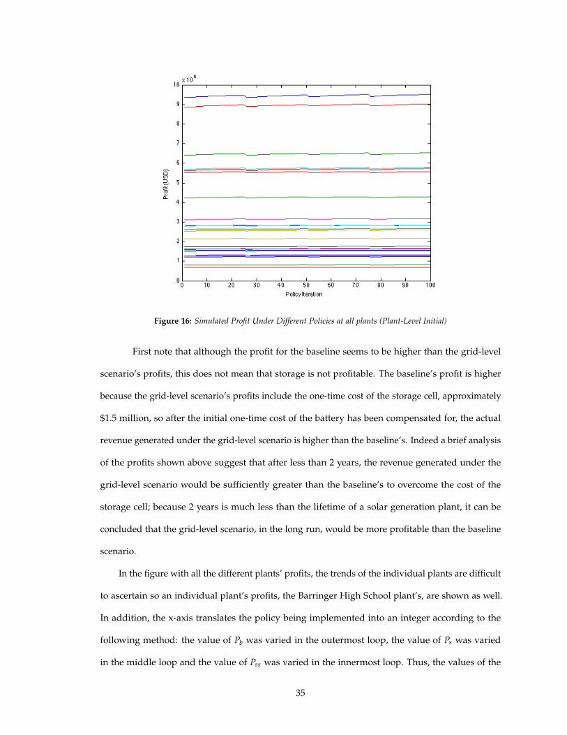
Figure 16: Simulated Profit Under Different Policies at all plants (Plant-Level Initial)
First note that although the profit for the baseline seems to be higher than the grid-level
scenario’s profits, this does not mean that storage is not profitable. The baseline’s profit is higher
because the grid-level scenario’s profits include the one-time cost of the storage cell, approximately
$1.5 million, so after the initial one-time cost of the battery has been compensated for, the actual
revenue generated under the grid-level scenario is higher than the baseline’s. Indeed a brief analysis
of the profits shown above suggest that after less than 2 years, the revenue generated under the
grid-level scenario would be sufficiently greater than the baseline’s to overcome the cost of the
storage cell; because 2 years is much less than the lifetime of a solar generation plant, it can be
concluded that the grid-level scenario, in the long run, would be more profitable than the baseline
scenario.
In the figure with all the different plants’ profits, the trends of the individual plants are difficult
to ascertain so an individual plant’s profits, the Barringer High School plant’s, are shown as well.
In addition, the x-axis translates the policy being implemented into an integer according to the
following method: the value of Pb was varied in the outermost loop, the value of Ps was varied
in the middle loop and the value of Pss was varied in the innermost loop. Thus, the values of the
35

parameter given an iteration value k ∈ [1, 100] can be expressed as:
Pb = ~Pb(a) such that a =
⌈k
25
⌉, Ps = ~Ps(b) such that b =
⌈k mod 25
5
⌉
Pss = ~Pss(c) such that c =
k mod 5 if k mod 5 6= 0
5 else
As both the graph of grid-level storage profits and the Barringer High School solar generation
plant’s profits suggest, the optimal value for the parameters seem to be outside of the initial range.
This hypothesis is supported by the fact that the profits increase to the edge of the tested range of
parameters. Thus, the next step is to test a different range of parameter values. The next range of
parameter values tested by this work was:
Pb ∈ ~Pb = {4, 5, 6, 7, 8}
Ps ∈ ~Ps = {R(L0.5), R(L0.5) + 1, R(L0.5) + 2, R(L0.5) + 3, R(L0.5) + 4}
Pss ∈ ~Pss{R(L0.9), R(L0.9) + 1, R(L0.9) + 2, R(L0.9) + 3, R(L0.9) + 4}
Again, each set of possible parameter values is run on 10 different sets of solar generation
simulation values with the profits averaged. The results of running both dynamic programs with
the second set of parameter values described above, as well as side-by-side comparisons of the
results with the results from the previous parameter values are shown in the following table and
figures (note that the units of the values in the table are USD):
Summed Generation Individual Generations
Maximum Profit 4903300 7777200
Table 4: Maximized Profits under the two Scenarios (2nd Run)
36
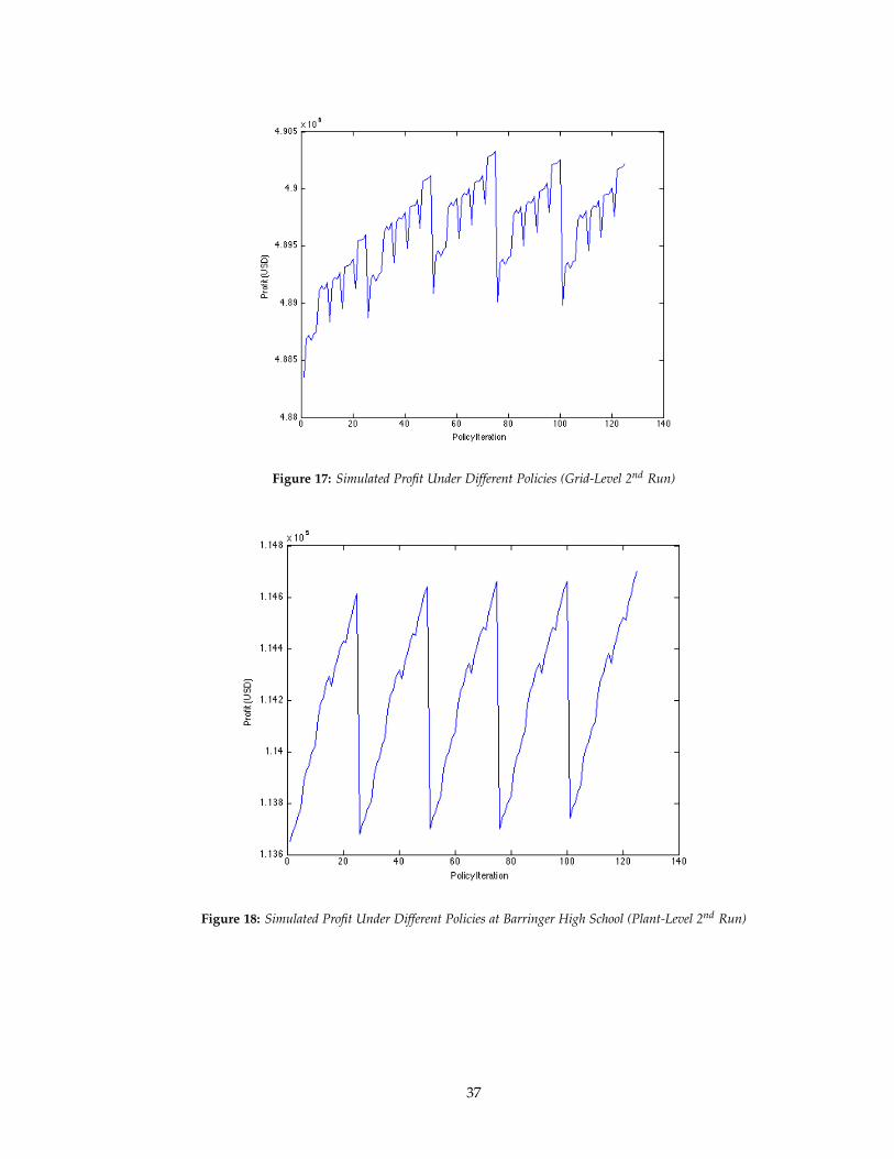
Figure 17: Simulated Profit Under Different Policies (Grid-Level 2nd Run)
Figure 18: Simulated Profit Under Different Policies at Barringer High School (Plant-Level 2nd Run)
37
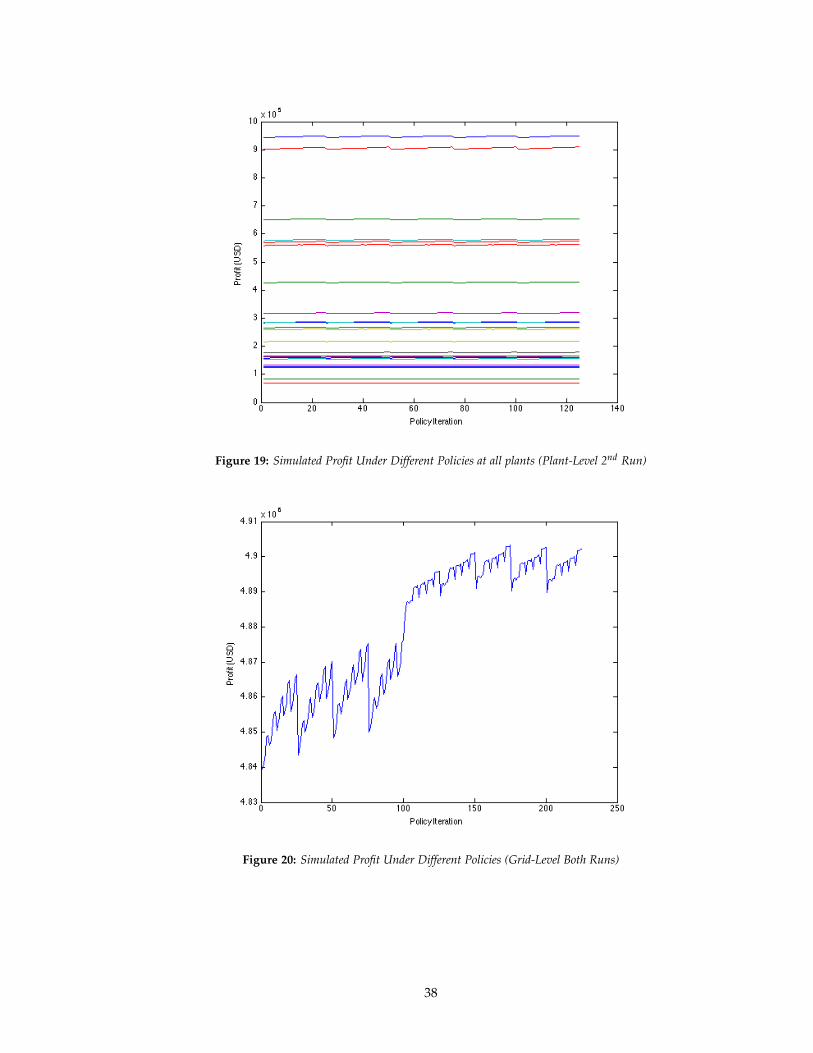
Figure 19: Simulated Profit Under Different Policies at all plants (Plant-Level 2nd Run)
Figure 20: Simulated Profit Under Different Policies (Grid-Level Both Runs)
38
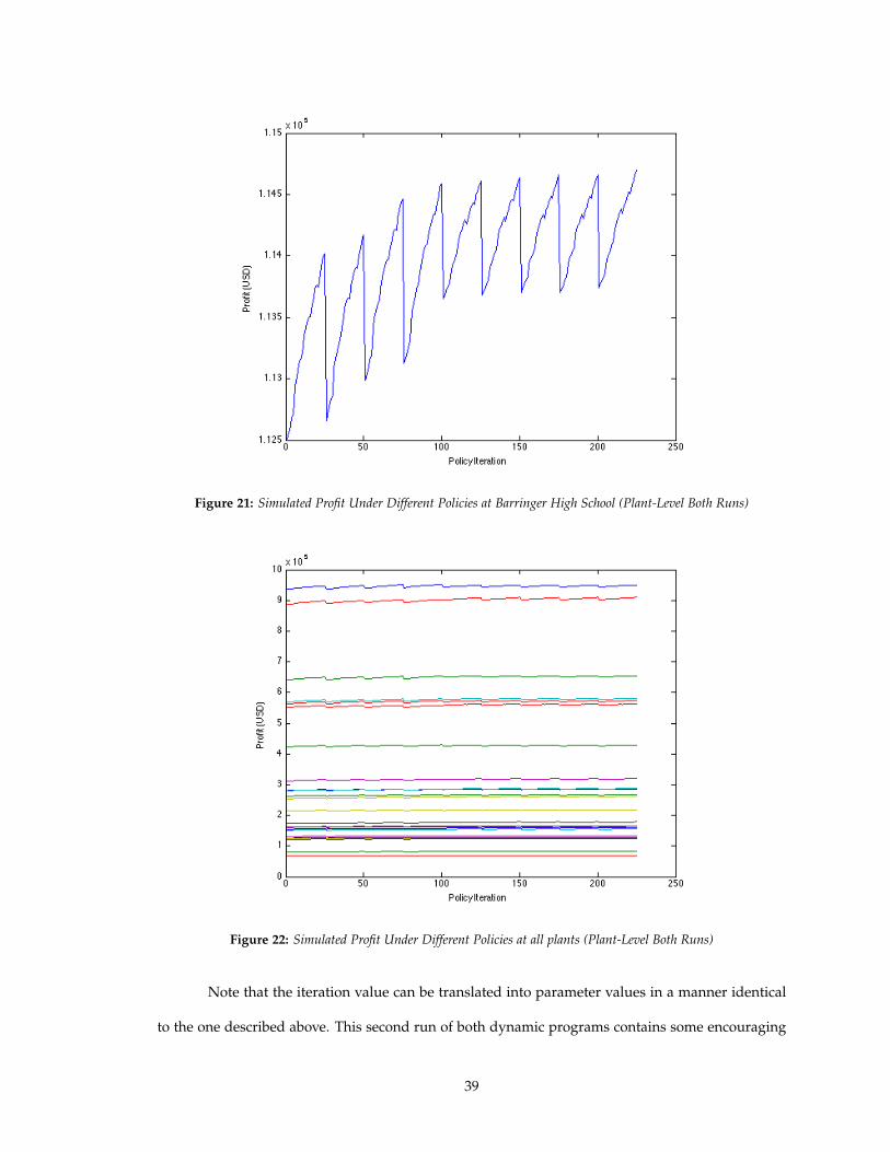
Figure 21: Simulated Profit Under Different Policies at Barringer High School (Plant-Level Both Runs)
Figure 22: Simulated Profit Under Different Policies at all plants (Plant-Level Both Runs)
Note that the iteration value can be translated into parameter values in a manner identical
to the one described above. This second run of both dynamic programs contains some encouraging
39

results: from figure 17, it is possible to see that a seeming optimum for Pb, at least given the ranges
of Ps and Pss, has been found to occur at Pb = 6. This statement is justified in that holding Ps and
Pss constant at any value in their respective parameter ranges, Pb = 6 maximizes the profit under
the summed generation scenario. Thus, in the ongoing search for the optimal parameter values,
the 3rd run of both dynamic programs consists of holding Pb constant at 6 and increasing Ps and
Pss in the following ranges:
Ps ∈ ~Ps = {R(L0.5) + 5, R(L0.5) + 6, R(L0.5) + 7, R(L0.5) + 8, R(L0.5) + 9,
R(L0.5) + 10, R(L0.5) + 11, R(L0.5) + 12, R(L0.5) + 13, R(L0.5) + 14}
Pss ∈ ~Pss{R(L0.9) + 5, R(L0.9) + 6, R(L0.9) + 7, R(L0.9) + 8, R(L0.9)
+9, R(L0.9) + 10, R(L0.9) + 11, R(L0.9) + 12, R(L0.9) + 13, R(L0.9) + 14}
Because Pb has been fixed at a certain value, the range over which both Ps and Pss can be
increased without drastically affecting the dynamic program’s runtime. However, this does affect
the way in which parameter values are calculated from an iteration value k:
Ps = ~Ps(a) such that a =
⌈k
10
⌉
Pss = ~Pss(b) such that b =
k mod 10 if k mod 10 6= 0
10 else
The following figures and table show the results of running the dynamic programs using the fixed
Pb and Ps, Pss in the ranges described above (note that the units of the values in the table are USD):
Summed Generation Individual Generations
Maximum Profit 4930900 7825200
Table 5: Maximized Profits under the two Scenarios (3rd Run)
40
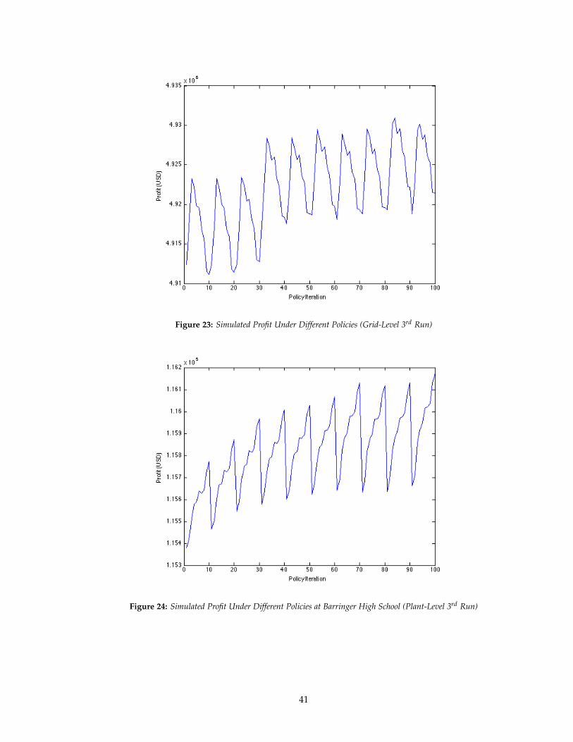
Figure 23: Simulated Profit Under Different Policies (Grid-Level 3rd Run)
Figure 24: Simulated Profit Under Different Policies at Barringer High School (Plant-Level 3rd Run)
41
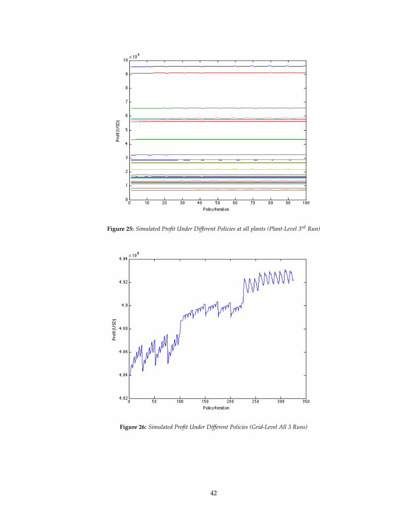
Figure 25: Simulated Profit Under Different Policies at all plants (Plant-Level 3rd Run)
Figure 26: Simulated Profit Under Different Policies (Grid-Level All 3 Runs)
42
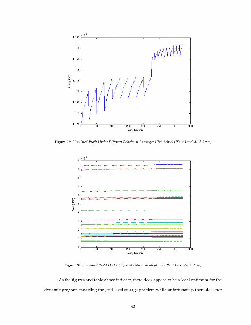
Figure 27: Simulated Profit Under Different Policies at Barringer High School (Plant-Level All 3 Runs)
Figure 28: Simulated Profit Under Different Policies at all plants (Plant-Level All 3 Runs)
As the figures and table above indicate, there does appear to be a local optimum for the
dynamic program modeling the grid-level storage problem while unfortunately, there does not
43
seem to be a local optimum for the plant-level storage dynamic program. The local optimum of the
grid-level dynamic program appears at iteration value 83, which translates to the parameter values
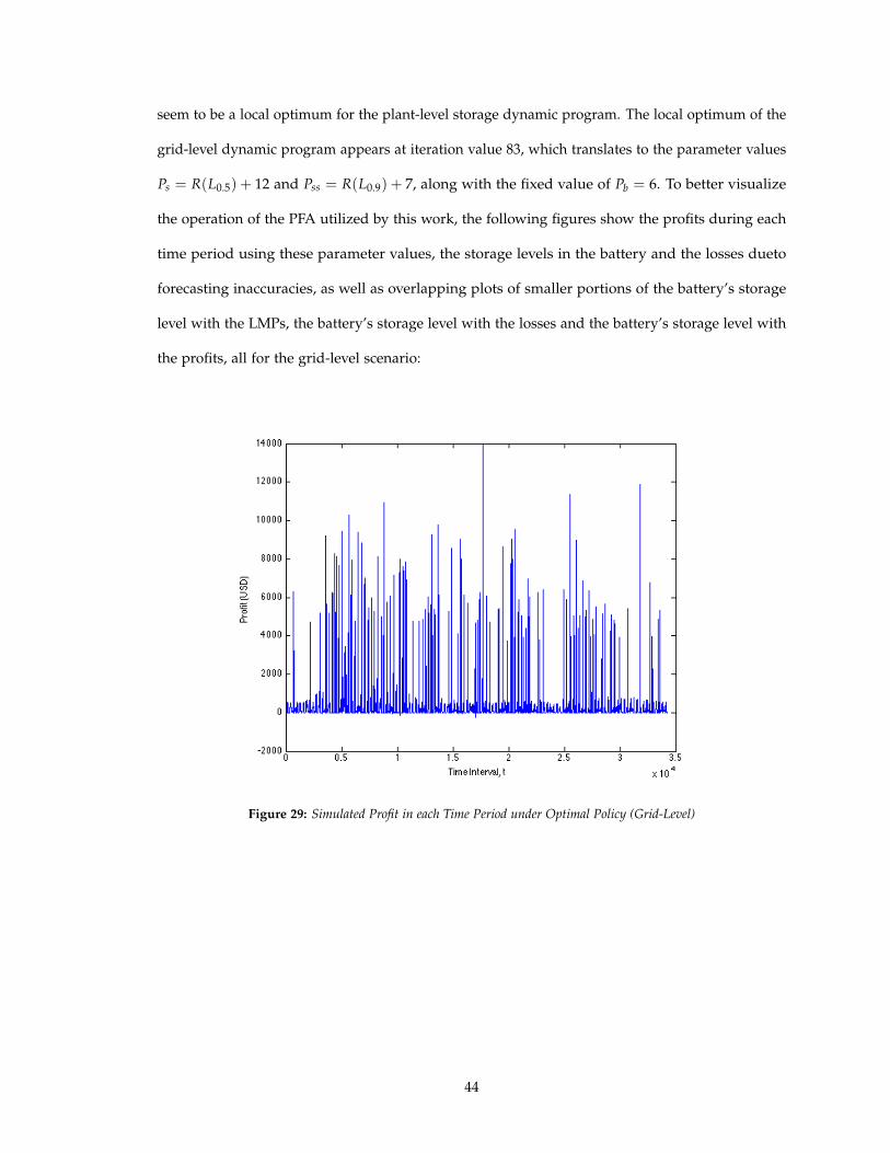
Ps = R(L0.5) + 12 and Pss = R(L0.9) + 7, along with the fixed value of Pb = 6. To better visualize
the operation of the PFA utilized by this work, the following figures show the profits during each
time period using these parameter values, the storage levels in the battery and the losses dueto
forecasting inaccuracies, as well as overlapping plots of smaller portions of the battery’s storage
level with the LMPs, the battery’s storage level with the losses and the battery’s storage level with
the profits, all for the grid-level scenario:
Figure 29: Simulated Profit in each Time Period under Optimal Policy (Grid-Level)
44
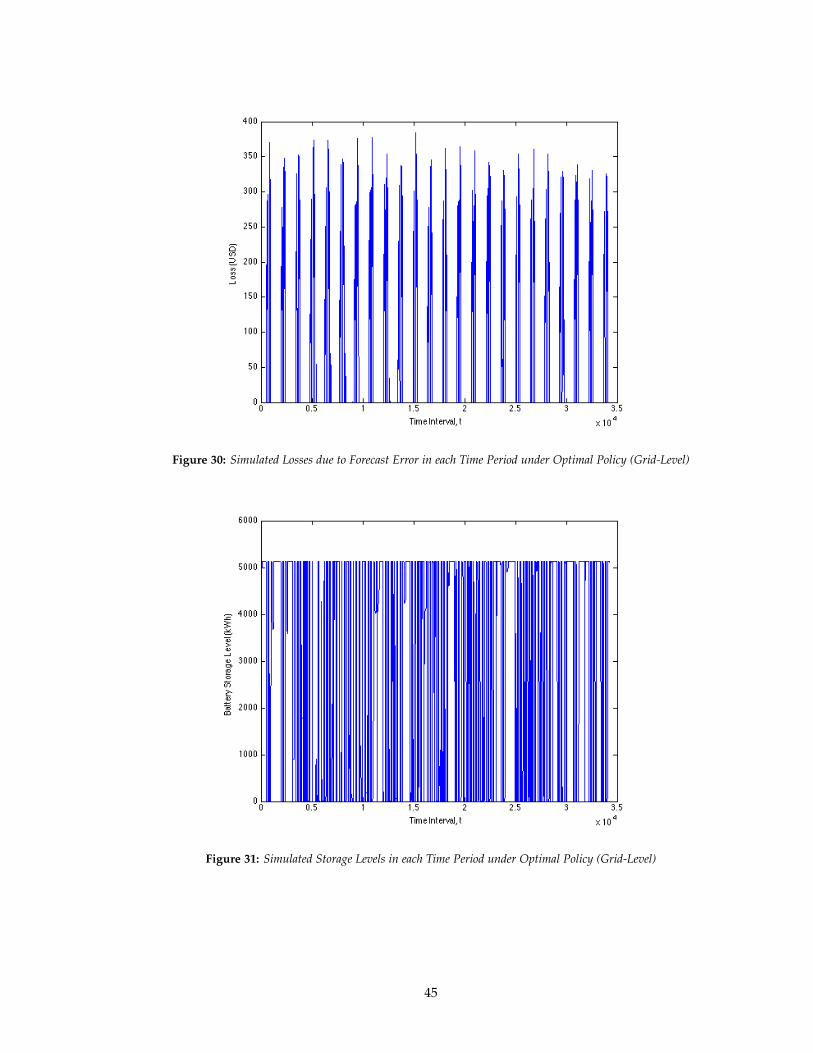
Figure 30: Simulated Losses due to Forecast Error in each Time Period under Optimal Policy (Grid-Level)
Figure 31: Simulated Storage Levels in each Time Period under Optimal Policy (Grid-Level)
45
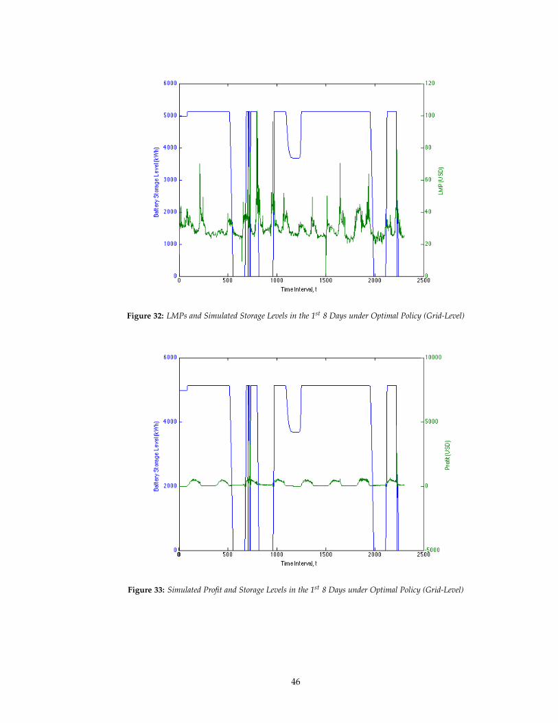
Figure 32: LMPs and Simulated Storage Levels in the 1st 8 Days under Optimal Policy (Grid-Level)
Figure 33: Simulated Profit and Storage Levels in the 1st 8 Days under Optimal Policy (Grid-Level)
46
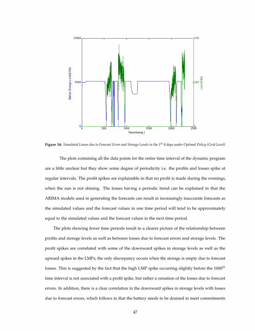
Figure 34: Simulated Losses due to Forecast Error and Storage Levels in the 1st 8 days under Optimal Policy (Grid-Level)
The plots containing all the data points for the entire time interval of the dynamic program
are a little unclear but they show some degree of periodicity i.e. the profits and losses spike at
regular intervals. The profit spikes are explainable in that no profit is made during the evenings,
when the sun is not shining. The losses having a periodic trend can be explained in that the
ARIMA models used in generating the forecasts can result in increasingly inaccurate forecasts as
the simulated values and the forecast values in one time period will tend to be approximately
equal to the simulated values and the forecast values in the next time period.
The plots showing fewer time periods result in a clearer picture of the relationship between
profits and storage levels as well as between losses due to forecast errors and storage levels. The
profit spikes are correlated with some of the downward spikes in storage levels as well as the
upward spikes in the LMPs; the only discrepancy occurs when the storage is empty due to forecast
losses. This is suggested by the fact that the high LMP spike occurring slightly before the 1000th
time interval is not associated with a profit spike, but rather a cessation of the losses due to forecast
errors. In addition, there is a clear correlation in the downward spikes in storage levels with losses
due to forecast errors, which follows in that the battery needs to be drained to meet commitments
47

that exceed the actual generation and will need to stay drained for as long as the forecast exceeds
the simulated generation values.
At this point in the analysis, it is worth noting that despite the constant improvements of
both dynamic programs, the maximized profit of the grid-level dynamic program in each run is
always much less than the maximized profit of the plant-level dynamic program, with the grid-level
dynamic program’s maximized profit hovering around 63% of the plant-level dynamic program’s
maximized profit. Thus, it can be said that the profit attainable under the particular policy function
approximation used by this work is greater for the scenario consisting of many smaller batteries,
each associated with a single solar generation plant than for the scenario consisting of a single
larger battery, despite the fact that the single battery’s capacity is much larger than the total capacity
of all the smaller batteries. The flexibility associated with independent policies for each smaller
battery appears to be a sufficiently beneficial factor to overcome the size differential.
48

6. Conclusions and Further Research
The results of this work suggest that the optimal strategy for utilities providers interested
in utilizing storage in conjunction with solar energy generation is to pair smaller storage cells
with individual solar generation plants as opposed to employing a single, larger storage cell. The
added benefit of allowing for the independent operation of the batteries opens up more complex
strategies that result in higher profits. This is of course constrained to the very specific operation of
the particular type of battery concerned in this work as well as operation in accord with the PFA
described in Section 2.2.6. However, the size of the gap in maximized profits suggests that even out-
side of these specific constraints, the plant-level scenario will still outperform the grid-level scenario.
6.1. Physical Constraints of the Storage Model
The model of electrical storage used in this work is very basic: of the relevant physical con-
straints that batteries are subject to, this model only considers the capacity constraint and the round
trip efficiency factors. In addition to these, the physics of chemical storage also adds restrictions
on the minimum percentage to which a battery can be safely discharged as well as the maximum
possible rate of electrical discharge and a self-discharge rate i.e. the rate at which electricity is
lost from the battery overtime. Brunet states that for a stationary lead-acid battery, the battery
should never be discharged below 20% of its maximum capacity and the self-discharge rate is
approximately 2% of its maximum capacity per month while its maximum discharge rate is the
battery’s maximum capacity divided by 10 hours.
In addition, the constraints described above and the constraints used by this work only apply
to the commonly utilized stationary, lead-acid battery. These values would be different for more
advanced, less common types of batteries. Thus, one potential extension of this work would be to
49
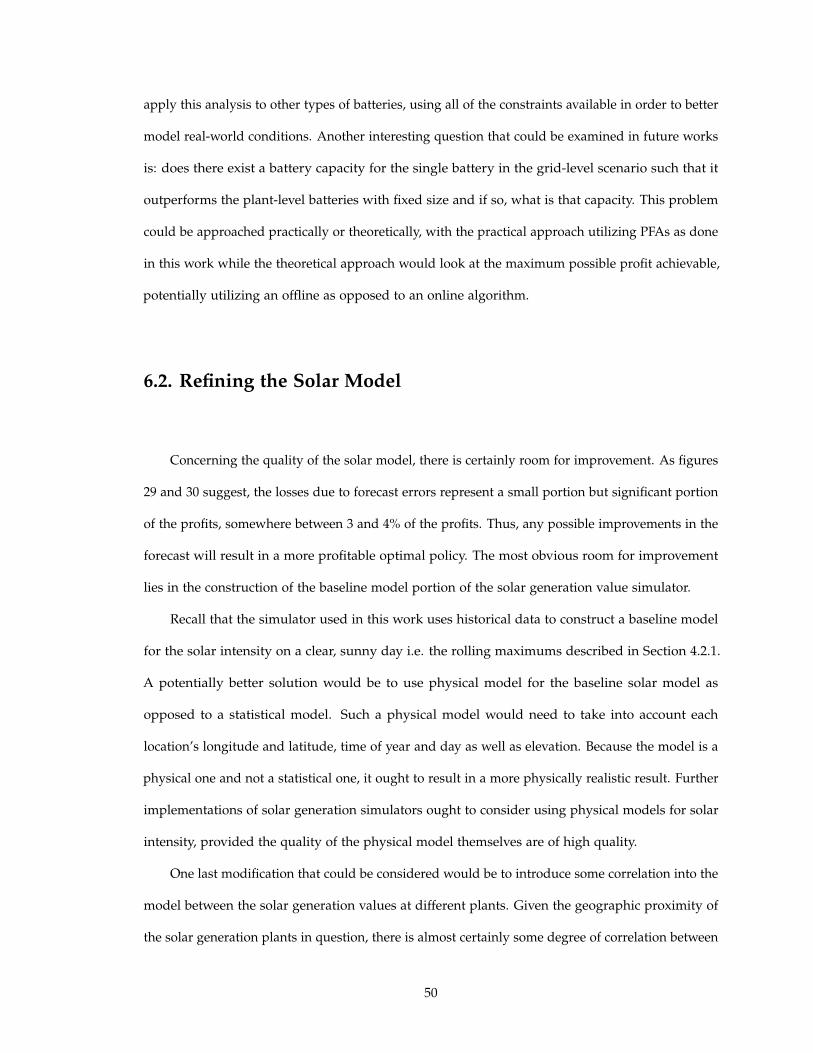
apply this analysis to other types of batteries, using all of the constraints available in order to better
model real-world conditions. Another interesting question that could be examined in future works
is: does there exist a battery capacity for the single battery in the grid-level scenario such that it
outperforms the plant-level batteries with fixed size and if so, what is that capacity. This problem
could be approached practically or theoretically, with the practical approach utilizing PFAs as done
in this work while the theoretical approach would look at the maximum possible profit achievable,
potentially utilizing an offline as opposed to an online algorithm.
6.2. Refining the Solar Model
Concerning the quality of the solar model, there is certainly room for improvement. As figures
29 and 30 suggest, the losses due to forecast errors represent a small portion but significant portion
of the profits, somewhere between 3 and 4% of the profits. Thus, any possible improvements in the
forecast will result in a more profitable optimal policy. The most obvious room for improvement
lies in the construction of the baseline model portion of the solar generation value simulator.
Recall that the simulator used in this work uses historical data to construct a baseline model
for the solar intensity on a clear, sunny day i.e. the rolling maximums described in Section 4.2.1.
A potentially better solution would be to use physical model for the baseline solar model as
opposed to a statistical model. Such a physical model would need to take into account each
location’s longitude and latitude, time of year and day as well as elevation. Because the model is a
physical one and not a statistical one, it ought to result in a more physically realistic result. Further
implementations of solar generation simulators ought to consider using physical models for solar
intensity, provided the quality of the physical model themselves are of high quality.
One last modification that could be considered would be to introduce some correlation into the
model between the solar generation values at different plants. Given the geographic proximity of
the solar generation plants in question, there is almost certainly some degree of correlation between
50

solar intensities at each location. As the models being simulated are time series, the inclusion of
correlation would no doubt employ the estimation of cross-correlation functions and then factoring
that into the simulation of generation values. The consideration of correlation between locations
could allow for a more realistic simulation.
6.3. Final Remarks
The results of this work show that solar energy can be profitably integrated into the PJM
market. One of the major reasons why the current penetration of renewables in electricity grids is
low is because of imposing start-up costs and the low profitability of renewable energy ventures
due to the volatility of renewable resources. The coupling of renewables with storage as well as
refinements in forecasting techniques will encourage greater utilization of renewables in the future,
a necessary task as the limited fossil fuel resources of Earth are used up. Both of these aspects are
explored in this work but of course, there are many possible improvements that can be made to
refine the analysis done here, some of which are described in this section. In conclusion, the results
of this work suggest that it is more profitable to utilize many smaller batteries than a single, larger
battery in conjunction with renewable energy production.
51

References
Box, George and Gwilym Jenkins. ”Time Series Analysis: Forecast and Control” Holden Day,1976.
Brockwell, Peter J. and Richard A. Davis. ”Time Series: Theory and Methods” Springer Series inStatistics, 1991.
Brunet, Yves. ”Energy Storage” John Wiley & Sons Inc., 2011.
Costa, Luıs M. and Franck Bourry, Jeremie Juban, George Kariniotakis. ”Management ofEnergy Storage Coordinated with Wind Power under Electricity Market Conditions” Paperpresented at IEEE 10th International Conference on Probabilistic Methods Applied to PowerSystems, 25 May, 2008.
Database of State Incentives for Renewables & Efficiency (DSIRE). ”New Jersey: Incentives/Policiesfor Renewables & Efficiency” U.S. Department of Energy ,28 Mar., 2013. http://www.dsireusa.org/incentives/incentive.cfm?Incentive Code =NJ05R
Friedman, Alexi. ”N.J. regulators approve PSE&G’s $446 million plan for solar farms atop landfills,brownfields” The Star-Ledger, 29 May, 2013. http://www.nj.com/ business/index.ssf/2013/05/nj regulators approve psegs 44.html
Huang, Rui and Tiana Huang, Na Li, Rajit Gadh. ”Solar Generation Prediction using the ARMAmodel in a Laboratory-Level Micro-grid” Paper presented at IEEE Third InternationalConference on Digital Object Identifier, 5 Nov., 2012.
Jin, Yinzhen. ”A stochastic model of errors in wind forecasts” Dissertation, PrincetonUniversity, May 2013.
Kassaveri, Rajesh and Krithika Seetharaman. ”Day-ahead wind speed forecasting using f-ARIMAmodels” Renewable Energy 34.5 (2009): 1388-1393.
Kim, Jae Ho, and Warren B. Powell. ”Optimal energy commitments with storage andintermittent supply” Operations Research 59.6 (2011): 1347-1360. Web. 20 Sep., 2013.
Lopez, Anthony and Billy Roberts, Donna Heimiller, Nate Blair, Gian Porro. ”U.S. RenewableEnergy Technical Potentials: A GIS-Based Analysis” National Renewable Energy LaboratoryJuly 2012. http://www.nrel.gov/docs/fy12osti/51946.pdf
Meza, Edgar. ”US surpasses 5 GW of utility-scale solar capacity” PV Magazine, 14 Jan., 2014.http://www.pv-magazine.com/news/details/beitrag/us-surpasses-5-gw-of- utility-scale-solar-capacity 100013933/#axzz2tvEb04cP
52

National Renewable Energy Laboratory (NREL). ”Open PV State Rankings” 2013. https://openpv.nrel.gov/rankings
National Renewable Energy Laboratory (NREL). ”Variability of Renewable Energy Sources” 25Mar., 2013. http://www.nrel.gov/electricity/transmission/variability.html
Powell, Warren B. ”Approximate Dynamic Programming: Solving the Curses ofDimensionality” John Wiley & Sons Inc., 2010.
Sandia National Laboratory (SNL). ”DOE Global Energy Storage Database” US Department ofEnergy, 2012. http://www.energystorageexchange.org/projects
Scott, Warren R., and Warren B. Powell. ”Approximate dynamic programming for energystorage with new results on instrumental variables and projected Bellman errors” Submittedto Operations Research (Under Review).
Solar Energy Industries Association (SEIA). ”U.S. PV Market Installs 930 Megawatts in Q3 2013;Second Largest Quarter Ever” 2013. http://www.seia.org/research-resources/ solar-industry-data
53

Appendix: Code Overview
There are two major uses for code in this work: the simulation of solar generation val-
ues and the running of the two dynamic programs. The code written to convert the raw data into
the z-scores used to fit ARIMA/ARMA models was written in Matlab, the simulator code was
written in R while the dynamic program code was written in Matlab.
Note that only the relevant code has been included in this Appendix. The excluded code
includes code run to preprocess the raw data, the code used to run multipler iterations of the
dynamic program and averages the results as well as the code run to generate the figures included
in this work. All of the figures in this work were generated in Matlab using calls to the built in
Matlab plot function.
54
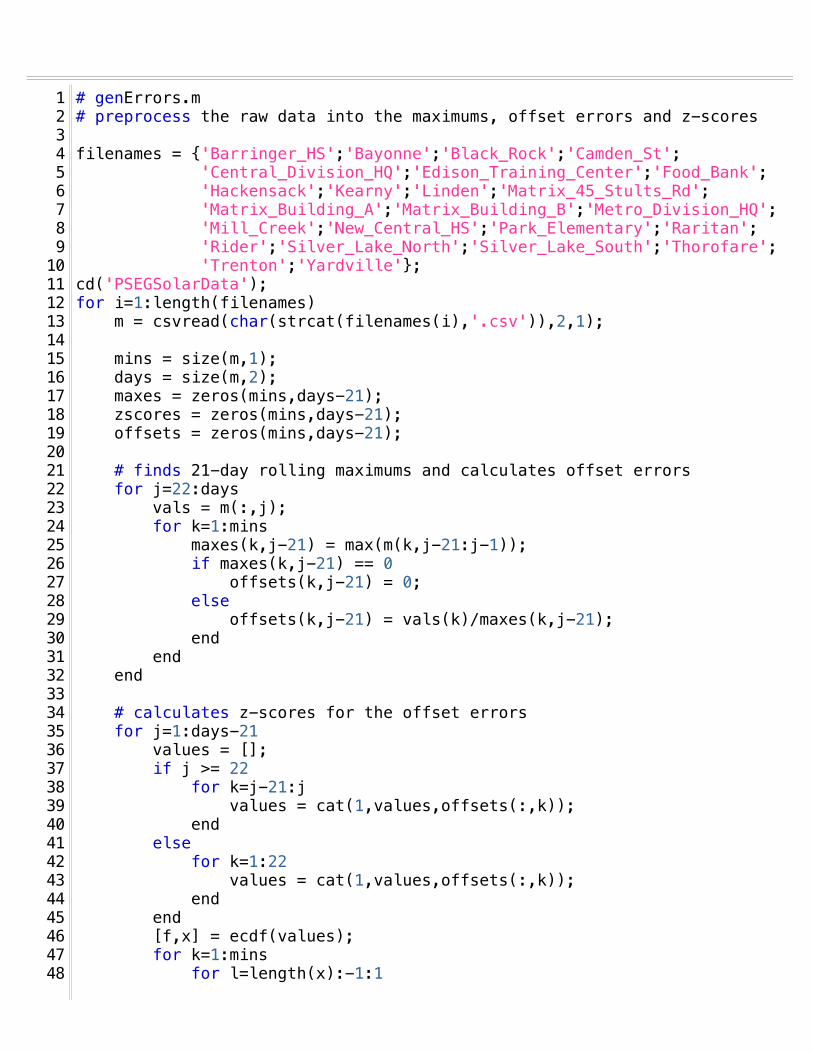
Page 1 of 2/Users/Chai/Desktop/Thesis/generrors_edit.mSaved: 4/8/14, 1:46:59 PM Printed For: Henry Chai
# genErrors.m1# preprocess the raw data into the maximums, offset errors and z-scores2
3filenames = {'Barringer_HS';'Bayonne';'Black_Rock';'Camden_St';4! ! ! 'Central_Division_HQ';'Edison_Training_Center';'Food_Bank';5! ! ! 'Hackensack';'Kearny';'Linden';'Matrix_45_Stults_Rd';6! ! ! 'Matrix_Building_A';'Matrix_Building_B';'Metro_Division_HQ';7! ! ! 'Mill_Creek';'New_Central_HS';'Park_Elementary';'Raritan';8! ! ! 'Rider';'Silver_Lake_North';'Silver_Lake_South';'Thorofare';9! ! ! 'Trenton';'Yardville'};10cd('PSEGSolarData');11for i=1:length(filenames)12 m = csvread(char(strcat(filenames(i),'.csv')),2,1);13 14 mins = size(m,1);15 days = size(m,2);16 maxes = zeros(mins,days-21);17 zscores = zeros(mins,days-21);18 offsets = zeros(mins,days-21);19 20 # finds 21-day rolling maximums and calculates offset errors21 for j=22:days22 vals = m(:,j);23 for k=1:mins24 maxes(k,j-21) = max(m(k,j-21:j-1));25 if maxes(k,j-21) == 026 offsets(k,j-21) = 0;27 else28 offsets(k,j-21) = vals(k)/maxes(k,j-21);29 end30 end31 end32 33 # calculates z-scores for the offset errors34 for j=1:days-21 35 values = [];36 if j >= 2237 for k=j-21:j38 values = cat(1,values,offsets(:,k));39 end40 else41 for k=1:2242 values = cat(1,values,offsets(:,k));43 end44 end45 [f,x] = ecdf(values);46 for k=1:mins47 for l=length(x):-1:148
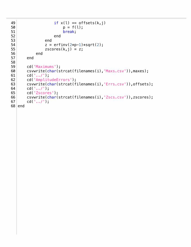
Page 2 of 2/Users/Chai/Desktop/Thesis/generrors_edit.mSaved: 4/8/14, 1:46:59 PM Printed For: Henry Chai
if x(l) == offsets(k,j)49 p = f(l);50 break;51 end52 end53 z = erfinv(2*p-1)*sqrt(2);54 zscores(k,j) = z;55 end56 end57 58 cd('Maximums');59 csvwrite(char(strcat(filenames(i),'Maxs.csv')),maxes);60 cd('../');61 cd('AmplitudeErrors');62 csvwrite(char(strcat(filenames(i),'Errs.csv')),offsets);63 cd('../');64 cd('Zscores');65 csvwrite(char(strcat(filenames(i),'Zscs.csv')),zscores);66 cd('../');67end68
69
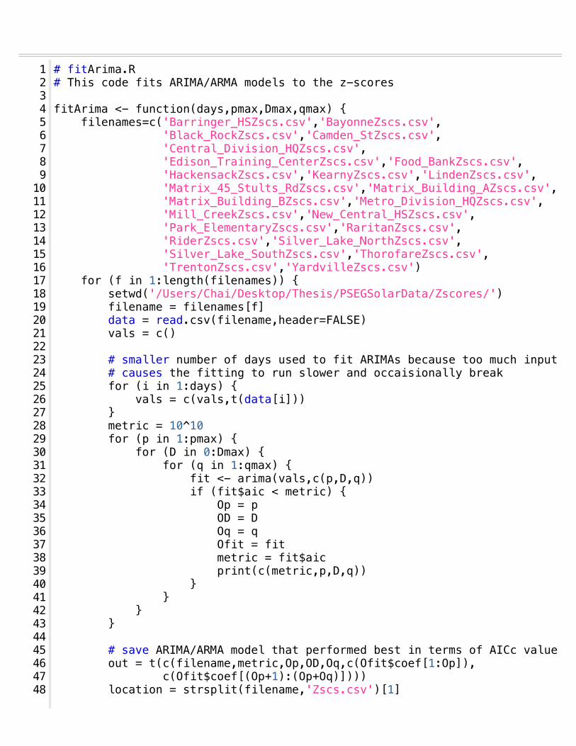
Page 1 of 2/Users/Chai/Desktop/Thesis/fitArima.RSaved: 4/8/14, 1:56:28 PM Printed For: Henry Chai
# fitArima.R1# This code fits ARIMA/ARMA models to the z-scores2
3fitArima <- function(days,pmax,Dmax,qmax) {4! filenames=c('Barringer_HSZscs.csv','BayonneZscs.csv',5! ! ! ! 'Black_RockZscs.csv','Camden_StZscs.csv',6! ! ! ! 'Central_Division_HQZscs.csv',7! ! ! ! 'Edison_Training_CenterZscs.csv','Food_BankZscs.csv',8! ! ! 'HackensackZscs.csv','KearnyZscs.csv','LindenZscs.csv',9! ! ! 'Matrix_45_Stults_RdZscs.csv','Matrix_Building_AZscs.csv',10! ! ! 'Matrix_Building_BZscs.csv','Metro_Division_HQZscs.csv',11! ! ! 'Mill_CreekZscs.csv','New_Central_HSZscs.csv',12! ! ! 'Park_ElementaryZscs.csv','RaritanZscs.csv',13! ! ! 'RiderZscs.csv','Silver_Lake_NorthZscs.csv',14! ! ! 'Silver_Lake_SouthZscs.csv','ThorofareZscs.csv',15! ! ! 'TrentonZscs.csv','YardvilleZscs.csv')16! for (f in 1:length(filenames)) {17! ! setwd('/Users/Chai/Desktop/Thesis/PSEGSolarData/Zscores/')18! ! filename = filenames[f]19! ! data = read.csv(filename,header=FALSE)20! ! vals = c()21! !22! ! # smaller number of days used to fit ARIMAs because too much input 23! ! # causes the fitting to run slower and occaisionally break24! ! for (i in 1:days) {25! ! ! vals = c(vals,t(data[i]))26! ! }27! ! metric = 10^1028! ! for (p in 1:pmax) {29! ! ! for (D in 0:Dmax) {30! ! ! ! for (q in 1:qmax) {31! ! ! ! ! fit <- arima(vals,c(p,D,q))32! ! ! ! ! if (fit$aic < metric) {33! ! ! ! ! ! Op = p34! ! ! ! ! ! OD = D35! ! ! ! ! ! Oq = q36! ! ! ! ! ! Ofit = fit37! ! ! ! ! ! metric = fit$aic38! ! ! ! ! ! print(c(metric,p,D,q))39! ! ! ! ! }40! ! ! ! }41! ! ! }42! ! }43! !44! ! # save ARIMA/ARMA model that performed best in terms of AICc value45! ! out = t(c(filename,metric,Op,OD,Oq,c(Ofit$coef[1:Op]),46! ! ! c(Ofit$coef[(Op+1):(Op+Oq)])))47! ! location = strsplit(filename,'Zscs.csv')[1]48

Page 2 of 2/Users/Chai/Desktop/Thesis/fitArima.RSaved: 4/8/14, 1:56:28 PM Printed For: Henry Chai
! ! setwd('/Users/Chai/Desktop/Thesis/PolicyEval')49! ! write.csv(out,paste(location,'.csv',sep=''))50! }51! setwd('/Users/Chai/Desktop/Thesis/PolicyEval')52}53fitArima(5,5,1,5)54
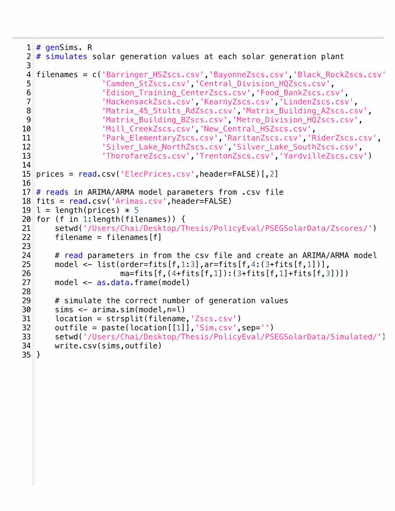
Page 1 of 1/Users/Chai/Desktop/Thesis/PolicyEval/genSims.RSaved: 4/8/14, 1:40:46 PM Printed For: Henry Chai
# genSims. R1# simulates solar generation values at each solar generation plant2
3filenames = c('Barringer_HSZscs.csv','BayonneZscs.csv','Black_RockZscs.csv',4! ! ! 'Camden_StZscs.csv','Central_Division_HQZscs.csv',5! ! ! 'Edison_Training_CenterZscs.csv','Food_BankZscs.csv',6! ! ! 'HackensackZscs.csv','KearnyZscs.csv','LindenZscs.csv',7! ! ! 'Matrix_45_Stults_RdZscs.csv','Matrix_Building_AZscs.csv',8! ! ! 'Matrix_Building_BZscs.csv','Metro_Division_HQZscs.csv',9! ! ! 'Mill_CreekZscs.csv','New_Central_HSZscs.csv',10! ! ! 'Park_ElementaryZscs.csv','RaritanZscs.csv','RiderZscs.csv',11! ! ! 'Silver_Lake_NorthZscs.csv','Silver_Lake_SouthZscs.csv',12! ! ! 'ThorofareZscs.csv','TrentonZscs.csv','YardvilleZscs.csv')13
14prices = read.csv('ElecPrices.csv',header=FALSE)[,2]15
16# reads in ARIMA/ARMA model parameters from .csv file17fits = read.csv('Arimas.csv',header=FALSE)18l = length(prices) * 519for (f in 1:length(filenames)) {20! setwd('/Users/Chai/Desktop/Thesis/PolicyEval/PSEGSolarData/Zscores/')21! filename = filenames[f]22!23! # read parameters in from the csv file and create an ARIMA/ARMA model24! model <- list(order=fits[f,1:3],ar=fits[f,4:(3+fits[f,1])],25! ! ! ! ma=fits[f,(4+fits[f,1]):(3+fits[f,1]+fits[f,3])])26! model <- as.data.frame(model)27!28! # simulate the correct number of generation values29! sims <- arima.sim(model,n=l)30! location = strsplit(filename,'Zscs.csv')31! outfile = paste(location[[1]],'Sim.csv',sep='')32! setwd('/Users/Chai/Desktop/Thesis/PolicyEval/PSEGSolarData/Simulated/')33! write.csv(sims,outfile)34}35
36
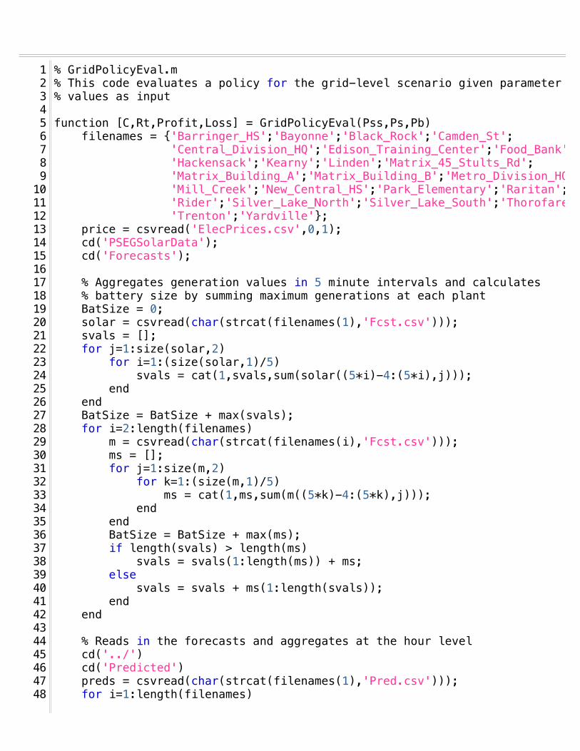
Page 1 of 3/Users/Chai/Desktop/Thesis/Thesis Document/Code/GridPolicyEval.mSaved: 4/8/14, 3:57:17 PM Printed For: Henry Chai
% GridPolicyEval.m1% This code evaluates a policy for the grid-level scenario given parameter 2% values as input3
4function [C,Rt,Profit,Loss] = GridPolicyEval(Pss,Ps,Pb) 5 filenames = {'Barringer_HS';'Bayonne';'Black_Rock';'Camden_St';6 ! ! ! 'Central_Division_HQ';'Edison_Training_Center';'Food_Bank';7 ! ! ! 'Hackensack';'Kearny';'Linden';'Matrix_45_Stults_Rd';8 ! ! ! 'Matrix_Building_A';'Matrix_Building_B';'Metro_Division_HQ';9 ! ! ! 'Mill_Creek';'New_Central_HS';'Park_Elementary';'Raritan';10 ! ! ! 'Rider';'Silver_Lake_North';'Silver_Lake_South';'Thorofare';11 ! ! ! 'Trenton';'Yardville'};12 price = csvread('ElecPrices.csv',0,1);13 cd('PSEGSolarData');14 cd('Forecasts');15 16 % Aggregates generation values in 5 minute intervals and calculates 17 % battery size by summing maximum generations at each plant 18 BatSize = 0;19 solar = csvread(char(strcat(filenames(1),'Fcst.csv')));20 svals = [];21 for j=1:size(solar,2)22 for i=1:(size(solar,1)/5)23 svals = cat(1,svals,sum(solar((5*i)-4:(5*i),j)));24 end25 end26 BatSize = BatSize + max(svals);27 for i=2:length(filenames)28 m = csvread(char(strcat(filenames(i),'Fcst.csv')));29 ms = [];30 for j=1:size(m,2)31 for k=1:(size(m,1)/5)32 ms = cat(1,ms,sum(m((5*k)-4:(5*k),j)));33 end34 end35 BatSize = BatSize + max(ms);36 if length(svals) > length(ms)37 svals = svals(1:length(ms)) + ms;38 else39 svals = svals + ms(1:length(svals));40 end41 end42 43 % Reads in the forecasts and aggregates at the hour level44 cd('../')45 cd('Predicted')46 preds = csvread(char(strcat(filenames(1),'Pred.csv')));47 for i=1:length(filenames)48
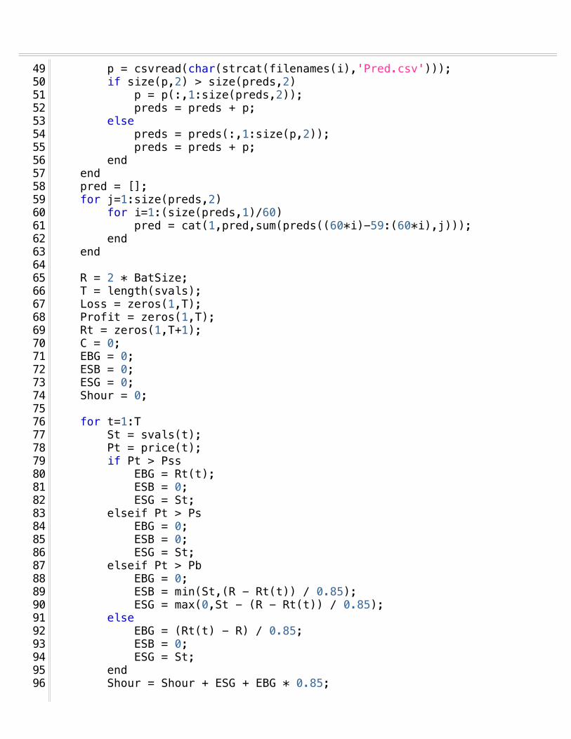
Page 2 of 3/Users/Chai/Desktop/Thesis/Thesis Document/Code/GridPolicyEval.mSaved: 4/8/14, 3:57:17 PM Printed For: Henry Chai
p = csvread(char(strcat(filenames(i),'Pred.csv')));49 if size(p,2) > size(preds,2)50 p = p(:,1:size(preds,2));51 preds = preds + p;52 else53 preds = preds(:,1:size(p,2));54 preds = preds + p;55 end56 end57 pred = []; 58 for j=1:size(preds,2)59 for i=1:(size(preds,1)/60)60 pred = cat(1,pred,sum(preds((60*i)-59:(60*i),j)));61 end62 end 63 64 R = 2 * BatSize;65 T = length(svals);66 Loss = zeros(1,T);67 Profit = zeros(1,T);68 Rt = zeros(1,T+1);69 C = 0;70 EBG = 0;71 ESB = 0;72 ESG = 0;73! Shour = 0;74!75 for t=1:T76 St = svals(t);77 Pt = price(t);78 if Pt > Pss79 EBG = Rt(t);80 ESB = 0;81 ESG = St; 82 elseif Pt > Ps83 EBG = 0;84 ESB = 0;85 ESG = St;86 elseif Pt > Pb87 EBG = 0;88 ESB = min(St,(R - Rt(t)) / 0.85);89 ESG = max(0,St - (R - Rt(t)) / 0.85);90 else91 EBG = (Rt(t) - R) / 0.85;92 ESB = 0;93 ESG = St; 94 end95 Shour = Shour + ESG + EBG * 0.85;96
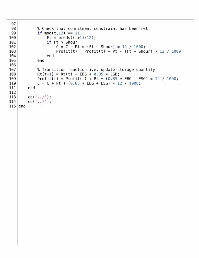
Page 3 of 3/Users/Chai/Desktop/Thesis/Thesis Document/Code/GridPolicyEval.mSaved: 4/8/14, 3:57:17 PM Printed For: Henry Chai
97 % Check that commitment constraint has been met98 if mod(t,12) == 1199 ! Ft = preds((t+1)/12);100 ! if Ft > Shour101! C = C - Pt * (Ft - Shour) * 12 / 1000;102 ! Profit(t) = Profit(t) - Pt * (Ft - Shour) * 12 / 1000;103! ! ! end104! ! end105! !106! ! % Transition function i.e. update storage quantity107 Rt(t+1) = Rt(t) - EBG + 0.85 * ESB;108 Profit(t) = Profit(t) + Pt * (0.85 * EBG + ESG) * 12 / 1000;109 C = C + Pt * (0.85 * EBG + ESG) * 12 / 1000;110 end111 112 cd('../');113 cd('../');114end115
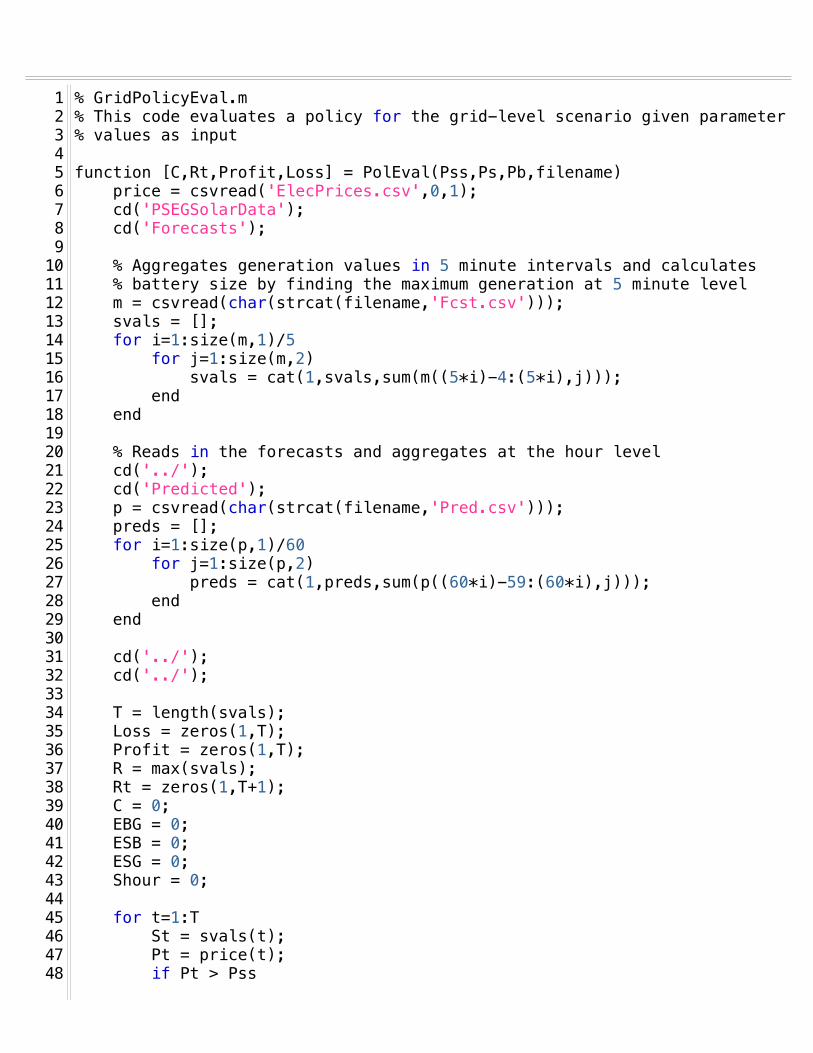
Page 1 of 2/Users/Chai/Desktop/Thesis/Thesis Document/Code/PlantPolicyEval.mSaved: 4/8/14, 4:00:22 PM Printed For: Henry Chai
% GridPolicyEval.m1% This code evaluates a policy for the grid-level scenario given parameter 2% values as input3
4function [C,Rt,Profit,Loss] = PolEval(Pss,Ps,Pb,filename)5 price = csvread('ElecPrices.csv',0,1);6 cd('PSEGSolarData');7 cd('Forecasts');8 9 % Aggregates generation values in 5 minute intervals and calculates 10 % battery size by finding the maximum generation at 5 minute level11 m = csvread(char(strcat(filename,'Fcst.csv')));12 svals = [];13 for i=1:size(m,1)/514 for j=1:size(m,2)15 svals = cat(1,svals,sum(m((5*i)-4:(5*i),j)));16 end17 end18 19 % Reads in the forecasts and aggregates at the hour level 20 cd('../');21 cd('Predicted');22 p = csvread(char(strcat(filename,'Pred.csv')));23 preds = [];24 for i=1:size(p,1)/6025 for j=1:size(p,2)26 preds = cat(1,preds,sum(p((60*i)-59:(60*i),j)));27 end28 end29 30 cd('../');31 cd('../');32
33 T = length(svals);34 Loss = zeros(1,T);35 Profit = zeros(1,T);36 R = max(svals);37 Rt = zeros(1,T+1);38 C = 0;39 EBG = 0;40 ESB = 0;41 ESG = 0;42! Shour = 0;43!44 for t=1:T45 St = svals(t);46 Pt = price(t);47 if Pt > Pss48
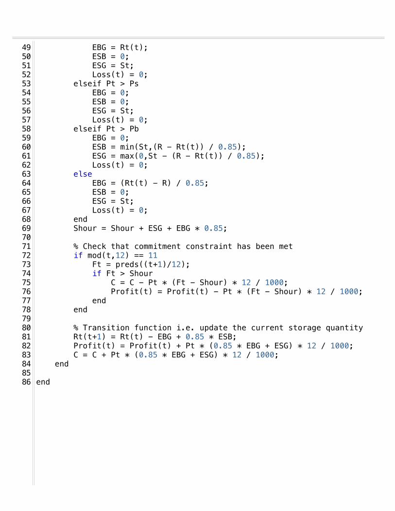
Page 2 of 2/Users/Chai/Desktop/Thesis/Thesis Document/Code/PlantPolicyEval.mSaved: 4/8/14, 4:00:22 PM Printed For: Henry Chai
EBG = Rt(t);49 ESB = 0;50 ESG = St; 51 Loss(t) = 0;52 elseif Pt > Ps53 EBG = 0;54 ESB = 0;55 ESG = St;56 Loss(t) = 0;57 elseif Pt > Pb58 EBG = 0;59 ESB = min(St,(R - Rt(t)) / 0.85);60 ESG = max(0,St - (R - Rt(t)) / 0.85);61 Loss(t) = 0;62 else63 EBG = (Rt(t) - R) / 0.85;64 ESB = 0;65 ESG = St; 66 Loss(t) = 0;67 end68 Shour = Shour + ESG + EBG * 0.85;69 70 % Check that commitment constraint has been met71 if mod(t,12) == 1172 ! Ft = preds((t+1)/12);73 ! if Ft > Shour74! C = C - Pt * (Ft - Shour) * 12 / 1000;75 ! Profit(t) = Profit(t) - Pt * (Ft - Shour) * 12 / 1000;76! ! ! end77! ! end78! !79! ! % Transition function i.e. update the current storage quantity80 Rt(t+1) = Rt(t) - EBG + 0.85 * ESB;81 Profit(t) = Profit(t) + Pt * (0.85 * EBG + ESG) * 12 / 1000;82 C = C + Pt * (0.85 * EBG + ESG) * 12 / 1000;83 end84 85end86
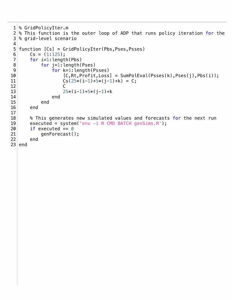
Page 1 of 1/Users/Chai/Desktop/Thesis/Thesis Document/Code/GridPolicyIter.mSaved: 4/8/14, 3:57:49 PM Printed For: Henry Chai
% GridPolicyIter.m1% This function is the outer loop of ADP that runs policy iteration for the2% grid-level scenario3
4function [Cs] = GridPolicyIter(Pbs,Pses,Psses)5 Cs = (1:125);6 for i=1:length(Pbs) 7 for j=1:length(Pses)8 for k=1:length(Psses)9 [C,Rt,Profit,Loss] = SumPolEval(Psses(k),Pses(j),Pbs(i));10 Cs(25*(i-1)+5*(j-1)+k) = C;11 C12 25*(i-1)+5*(j-1)+k13 end14 end15 end16!17! % This generates new simulated values and forecasts for the next run18 executed = system('env -i R CMD BATCH genSims.R');19 if executed == 020 genForecast();21 end22end23
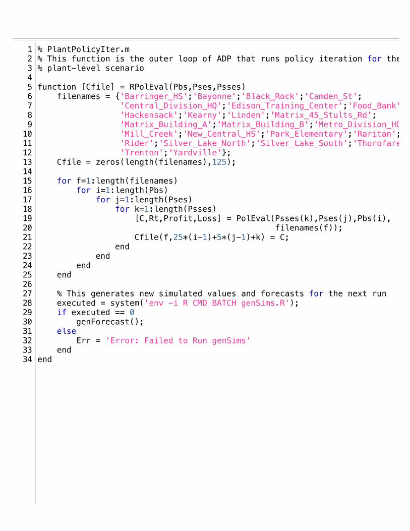
Page 1 of 1/Users/Chai/Desktop/Thesis/Thesis Document/Code/PlantPolicyIter.mSaved: 4/8/14, 3:13:33 PM Printed For: Henry Chai
% PlantPolicyIter.m1% This function is the outer loop of ADP that runs policy iteration for the2% plant-level scenario3
4function [Cfile] = RPolEval(Pbs,Pses,Psses)5 filenames = {'Barringer_HS';'Bayonne';'Black_Rock';'Camden_St';6 ! ! ! 'Central_Division_HQ';'Edison_Training_Center';'Food_Bank';7 ! ! ! 'Hackensack';'Kearny';'Linden';'Matrix_45_Stults_Rd';8 ! ! ! 'Matrix_Building_A';'Matrix_Building_B';'Metro_Division_HQ';9 ! ! ! 'Mill_Creek';'New_Central_HS';'Park_Elementary';'Raritan';10 ! ! ! 'Rider';'Silver_Lake_North';'Silver_Lake_South';'Thorofare';11 ! ! ! 'Trenton';'Yardville'};12 Cfile = zeros(length(filenames),125);13
14 for f=1:length(filenames)15 for i=1:length(Pbs) 16 for j=1:length(Pses)17 for k=1:length(Psses)18 [C,Rt,Profit,Loss] = PolEval(Psses(k),Pses(j),Pbs(i),19 ! ! ! ! ! ! ! filenames(f));20 Cfile(f,25*(i-1)+5*(j-1)+k) = C;21 end22 end23 end24 end25 26! % This generates new simulated values and forecasts for the next run!27 executed = system('env -i R CMD BATCH genSims.R');28 if executed == 029 genForecast();30 else31 Err = 'Error: Failed to Run genSims'32 end33end34
35


