

The solution of high dimensional elliptic PDEswith random data
Ivan Graham, University of Bath, UK.
Joint work with:
Frances Kuo, Ian Sloan (New South Wales)Dirk Nuyens (Leuven)Rob Scheichl (Bath)
CUHK April 2016

High dimensional Problems: PDE with random data
• Many problems involve PDEs with spatially varying datawhich is subject to uncertainty.
Example: groundwater flow in rock underground.
• Uncertainty enters the PDE through its coefficients. (randomfields). The quantity of interest: is a random number or fieldderived from the PDE solution.
Examples: (i) pressure in medium, (ii) effective permeability,(iii) breakthrough time of a pollution plume .
• Typical Computational Goal: expected value of quantity ofinterest.
This is the Forward problem of uncertainty quantification
Some ingredients
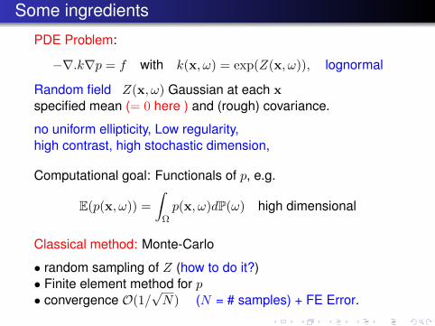
PDE Problem:
−∇.k∇p = f with k(x, ω) = exp(Z(x, ω)), lognormal
Random field Z(x, ω) Gaussian at each xspecified mean (= 0 here ) and (rough) covariance.
no uniform ellipticity, Low regularity,high contrast, high stochastic dimension,
Computational goal: Functionals of p, e.g.
E(p(x, ω)) =
∫Ωp(x, ω)dP(ω) high dimensional
Classical method: Monte-Carlo
• random sampling of Z (how to do it?)• Finite element method for p• convergence O(1/
√N) (N = # samples) + FE Error.
Outline of talk
Part I: Algorithm: circulant embedding with Quasi-Monte Carlo
IGG, Kuo, Nuyens, Scheichl, Sloan JCP 2011
Part II: Rigorous error estimates
IGG, Kuo, Nicholls, Scheichl, Schwab, SloanNumer Math 2014
IGG, Scheichl, UllmannStochastic PDE: Analysis and Computation 2014
IGG, Kuo, Nuyens, Scheichl, Sloan in preparation 2016
Gaussian Random Fields (more generally)
PDE Problem:
−∇.k∇p = f + Boundary conditions k = exp(Z)
Covariance function: (centred) stationary field:
E[Z(x, ·)Z(y, ·)] = ρ(x− y), ρ positive definite
Examples:ρ(x− y) = σ2 exp
(− ‖x− y‖/λ
)“exponential”.
ρ(x− y) = σ2 exp(− ‖x− y‖2/λ
)“Gaussian”.
σ2 = variance , λ = lengthscale
The Matern family: ρ = ρβ, β ∈ [1/2,∞).Limiting cases: exponential (β = 1/2), Gaussian (β =∞).

Gaussian Random Fields (more generally)
Loss of uniform ellipticity and boundedness: for all ε > 0:
min[P(k(x, ·) < ε), P(k(x, ·)) > ε−1)] > 0
Mild smoothness condition on ρ(0):Karhunen-Loeve (KL) Expansion: (a.s. convergence)
Z(x, ω) =
∞∑j=1
√µjξj(x)Yj(ω) Yj ∼ N(0, 1)
(ξj , µj) eigenpairs of covariance operator with kernel ρ(x− y).
Kolmogorov’s theorem: With probability 1,k(x, ω) ∈ Ct(D), with t ∈ [0, β)
In fact, for all q ∈ (1,∞),• k ∈ Lq(Ω, Ct(D)),• and ‖p‖Lq(Ω,H1
0 (D)) ≤ ‖a−1min‖Lq(Ω)‖f‖H−1 (Dirichlet problem).
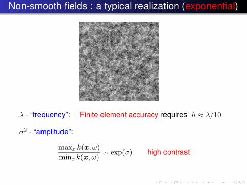
Non-smooth fields : a typical realization (exponential)
λ - “frequency”: Finite element accuracy requires h ≈ λ/10
σ2 - “amplitude”:
maxx k(x, ω)
minx k(x, ω)∼ exp(σ) high contrast
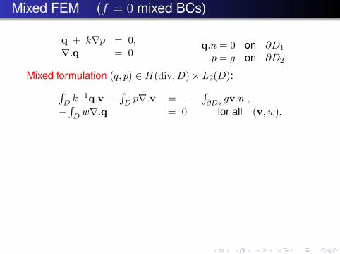
Mixed FEM (f = 0 mixed BCs)
q + k∇p = 0,∇.q = 0
q.n = 0 on ∂D1
p = g on ∂D2
Mixed formulation (q, p) ∈ H(div, D)× L2(D):∫D k−1q.v −
∫D p∇.v = −
∫∂D2
gv.n ,
−∫D w∇.q = 0 for all (v, w).
h = finite element grid size.
PC = Piecewise constants
Space RT0:qh = a + bx but divergence free =⇒ b = 0 .
Quadrature rule: sample k(x, ω) one point per elementEnough for accuracy:IGG, Scheichl, Ullmann,2015
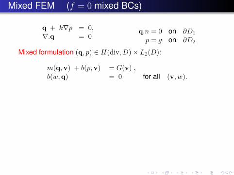
Mixed FEM (f = 0 mixed BCs)
q + k∇p = 0,∇.q = 0
q.n = 0 on ∂D1
p = g on ∂D2
Mixed formulation (q, p) ∈ H(div, D)× L2(D):
m(q,v) + b(p,v) = G(v) ,b(w,q) = 0 for all (v, w).
h = finite element grid size.
PC = Piecewise constants
Space RT0:qh = a + bx but divergence free =⇒ b = 0 .
Quadrature rule: sample k(x, ω) one point per elementEnough for accuracy:IGG, Scheichl, Ullmann,2015

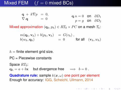
Mixed FEM (f = 0 mixed BCs)
q + k∇p = 0,∇.q = 0
q.n = 0 on ∂D1
p = g on ∂D2
Mixed approximation (qh, ph) ∈ RT0 × PC on a mesh Th:
m(qh,vh) + b(ph,vh) = G(vh) ,b(wh,qh) = 0 for all (vh, wh)
h = finite element grid size.
PC = Piecewise constants
Space RT0:qh = a + bx but divergence free =⇒ b = 0 .
Quadrature rule: sample k(x, ω) one point per elementEnough for accuracy:IGG, Scheichl, Ullmann,2015

Mixed FEM (f = 0 mixed BCs)
q + k∇p = 0,∇.q = 0
q.n = 0 on ∂D1
p = g on ∂D2
Mixed approximation (qh, ph) ∈ RT0 × PC on a mesh Th:
m(qh,vh) + b(ph,vh) = G(vh) ,b(wh,qh) = 0 for all (vh, wh)
h = finite element grid size.
PC = Piecewise constants
Space RT0:qh = a+ bx but divergence free =⇒ b = 0 .
Mixed FEM (f = 0 mixed BCs)
q + k∇p = 0,∇.q = 0
q.n = 0 on ∂D1
p = g on ∂D2
Mixed approximation (qh, ph) ∈ RT0 × PC on a mesh Th:
m(qh,vh) + b(ph,vh) = G(vh) ,b(wh,qh) = 0 for all (vh, wh)
h = finite element grid size.
PC = Piecewise constants
Space RT0:qh = a+ bx but divergence free =⇒ b = 0 .
Quadrature rule: sample k(x, ω) one point per elementEnough for accuracy: IGG, Scheichl, Ullmann, 2014
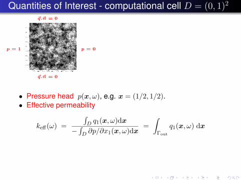
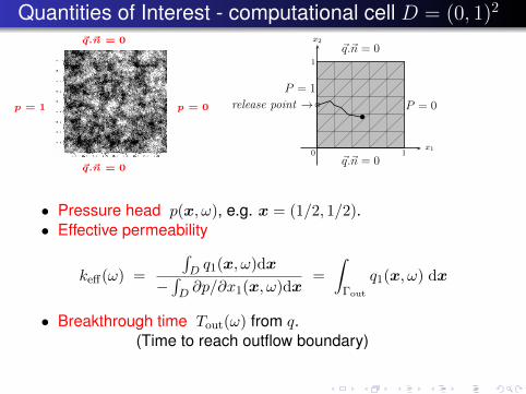
Quantities of Interest - computational cell D = (0, 1)2
p = 1 p = 0
~q.~n = 0
~q.~n = 0
1
• Pressure head p(x, ω), e.g. x = (1/2, 1/2).• Effective permeability
keff(ω) =
∫D q1(x, ω)dx
−∫D ∂p/∂x1(x, ω)dx
=
∫Γout
q1(x, ω) dx
Quantities of Interest - computational cell D = (0, 1)2
p = 1 p = 0
~q.~n = 0
~q.~n = 0
1
0
1
1x1
x2
P = 1
P = 0
~q.~n = 0
~q.~n = 0
release point →•
1
• Pressure head p(x, ω), e.g. x = (1/2, 1/2).• Effective permeability
keff(ω) =
∫D q1(x, ω)dx
−∫D ∂p/∂x1(x, ω)dx
=
∫Γout
q1(x, ω) dx
• Breakthrough time Tout(ω) from q.(Time to reach outflow boundary)
• General format: find E[G(p,q)] - some functional G(p,q).

Sampling by K-L truncation : the effect of lengthscale
Z(x, ω) =
∞∑j=1
√µjξj(x)Yj(ω)
exponential covariance in 1D
log log plot of µj for 1 ≤ j ≤ 500:
100 101 102 103
10−6
10−5
10−4
10−3
10−2
10−1
100
Plateau before decay starts
λ = 1λ = 0.1λ = 0.01
An extreme eigenvalue solverchallenge!
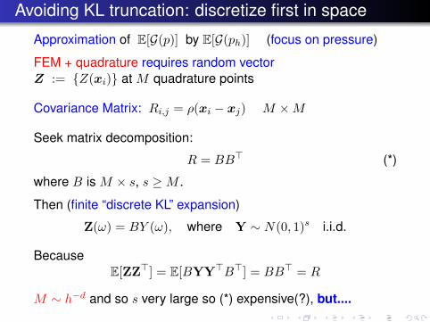
Avoiding KL truncation: discretize first in space
Approximation of E[G(p)] by E[G(ph)] (focus on pressure)
FEM + quadrature requires random vectorZ := Z(xi) at M quadrature points
Covariance Matrix: Ri,j = ρ(xi − xj) M ×M
Seek matrix decomposition:
R = BB> (*)
where B is M × s, s ≥M .
Then (finite “discrete KL” expansion)
Z(ω) = BY (ω), where Y ∼ N(0, 1)s i.i.d.
BecauseE[ZZ>] = E[BYY>B>] = BB> = R
M ∼ h−d and so s very large so (*) expensive(?), but....
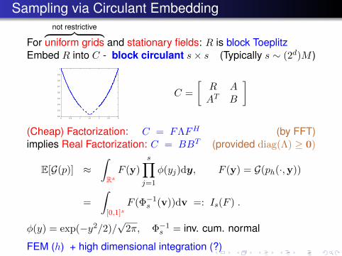
Sampling via Circulant Embedding
For
not restrictive︷ ︸︸ ︷uniform grids and stationary fields: R is block Toeplitz
Embed R into C - block circulant s× s (Typically s ∼ (2d)M )
0 0.5 1 1.5 2 2.5 30.2
0.3
0.4
0.5
0.6
0.7
0.8
0.9
1
C =
[R AAT B
]
(Cheap) Factorization: C = FΛFH (by FFT)implies Real Factorization: C = BBT (provided diag(Λ) ≥ 0)
E[G(p)] ≈∫RsF (y)
s∏j=1
φ(yj)dy, F (y) = G(ph(·,y))
=
∫[0,1]s
F (Φ−1s (v))dv =: Is(F ) .
φ(y) = exp(−y2/2)/√
2π, Φ−1s = inv. cum. normal
FEM (h) + high dimensional integration (?)

Integration over [0, 1]s (very large s): QMC methods
∫[0,1]s
f(z) dz ≈ 1
N
N∑k=1
f(z(k))
Monte Carlo methodz(k) random uniformO(N−1/2) convergenceorder of variables irrelevant
Quasi-Monte Carlo methodz(k) deterministicclose to O(N−1) convergenceorder of variables very important
64 random points
••
•
••
•
•
•
•
•
•
•••
•
•• •
•
•
•
•
•
•
•
•
•
•
•
•
•
•
•••
•
•
••
•
•
••
• ••
••
•
••
••
••
•
•
•
•
•
•
••
•
64 Sobol′ points•
•
•
•
•
•
•
••
•
•
•
•
•
•
•
•
•
•
•
•
•
•
••
•
•
•
•
•
•
•
•
•
•
•
•
•
•
••
•
•
•
•
•
•
•
•
•
•
•
•
•
•
••
•
•
•
•
•
•
•
64 lattice points•
•
•
•
•
•
•
•
•
•
•
•
•
•
•
•
•
•
•
•
•
•
•
•
•
•
•
•
•
•
•
•
•
•
•
•
•
•
•
•
•
•
•
•
•
•
•
•
•
•
•
•
•
•
•
•
•
•
•
•
•
•
•
•
1

Numerical Results
Covariance
r(x,y) = σ2 exp(− ‖x− y‖1/λ
).
( ‖ · ‖2 similar).
Case 1 Case 2 Case 3 Case 4 Case 5
σ2 = 1 σ2 = 1 σ2 = 1 σ2 = 3 σ2 = 3λ = 1 λ = 0.3 λ = 0.1 λ = 1 λ = 0.1
FEM: Uniform grid h = 1/m on (0, 1)2, M ∼ m2.
Sampling: circulant embedding via FFT (dimension s ≥ 4M )
High dimensional integration: QMC with N Sobol’ points

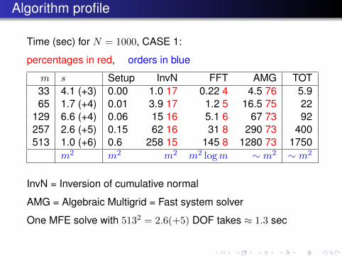
Algorithm profile
Time (sec) for N = 1000, CASE 1:
percentages in red, orders in blue
m s Setup InvN FFT AMG TOT33 4.1 (+3) 0.00 1.0 17 0.22 4 4.5 76 5.965 1.7 (+4) 0.01 3.9 17 1.2 5 16.5 75 22
129 6.6 (+4) 0.06 15 16 5.1 6 67 73 92257 2.6 (+5) 0.15 62 16 31 8 290 73 400513 1.0 (+6) 0.6 258 15 145 8 1280 73 1750
m2 m2 m2 m2 logm ∼ m2 ∼ m2
InvN = Inversion of cumulative normal
AMG = Algebraic Multigrid = Fast system solver
One MFE solve with 5132 = 2.6(+5) DOF takes ≈ 1.3 sec
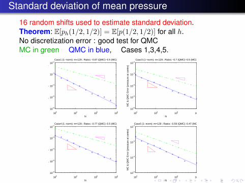
Standard deviation of mean pressure
16 random shifts used to estimate standard deviation.Theorem: E[ph(1/2, 1/2)] = E[p(1/2, 1/2)] for all h.No discretization error : good test for QMCMC in green QMC in blue, Cases 1,3,4,5.
103 104 105 106
10−6
10−5
10−4
10−3
10−2
N
MC
& Q
MC
Err
or (
pres
sure
at c
entr
e)
Case1 (1−norm): m=129 ; Rates:−0.87 (QMC)−0.5 (MC)
103 104 105 10
10−6
10−5
10−4
10−3
10−2
N
MC
& Q
MC
Err
or (
pres
sure
at c
entr
e)
Case3 (1−norm): m=129 ; Rates:−0.7 (QMC)−0.5 (MC)
103 104 105 106
10−6
10−5
10−4
10−3
10−2
N
MC
& Q
MC
Err
or (
pres
sure
at c
entr
e)
Case4 (1−norm): m=129 ; Rates:−0.77 (QMC)−0.5 (MC)
103 104 105 10
10−5
10−4
10−3
10−2
N
MC
& Q
MC
Err
or (
pres
sure
at c
entr
e)Case5 (1−norm): m=129 ; Rates:−0.59 (QMC)−0.47 (MC)

Dimension independence of QMC (and MC)
Standard deviation of mean pressure, Case 4:as m(= 1/h) (and hence s) increasesMC in green QMC in blue
103 104 105 106
10−6
10−5
10−4
10−3
10−2
N
MC
& Q
MC
Err
or (
pres
sure
at c
entr
e)
Case4 (1−norm): m=33 ; Rates:−0.78 (QMC)−0.5 (MC)
103 104 105 10
10−6
10−5
10−4
10−3
10−2
N
MC
& Q
MC
Err
or (
pres
sure
at c
entr
e)
Case4 (1−norm): m=65 ; Rates:−0.74 (QMC)−0.5 (MC)
103 104 105 106
10−6
10−5
10−4
10−3
10−2
N
MC
& Q
MC
Err
or (
pres
sure
at c
entr
e)
Case4 (1−norm): m=129 ; Rates:−0.77 (QMC)−0.5 (MC)
103 104 105 10
10−6
10−5
10−4
10−3
10−2
N
MC
& Q
MC
Err
or (
pres
sure
at c
entr
e)
Case4 (1−norm): m=257 ; Rates:−0.76 (QMC)−0.5 (MC)
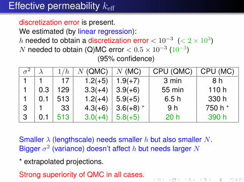
Effective permeability keff
discretization error is present.We estimated (by linear regression):h needed to obtain a discretization error < 10−3 (< 2× 10³)N needed to obtain (Q)MC error < 0.5× 10⁻³ (10−3)
(95% confidence)
σ2 λ 1/h N (QMC) N (MC) CPU (QMC) CPU (MC)1 1 17 1.2(+5) 1.9(+7) 3 min 8 h1 0.3 129 3.3(+4) 3.9(+6) 55 min 110 h1 0.1 513 1.2(+4) 5.9(+5) 6.5 h 330 h3 1 33 4.3(+6) 3.6(+8) ∗ 9 h 750 h ∗
3 0.1 513 3.0(+4) 5.8(+5) 20 h 390 h
Smaller λ (lengthscale) needs smaller h but also smaller N .Bigger σ2 (variance) doesn’t affect h but needs larger N
* extrapolated projections.
Strong superiority of QMC in all cases.
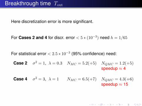
Breakthrough time Tout
Here discretization error is more significant.
For Cases 2 and 4 for discr. error < 5 ∗ (10−3) need h = 1/65
For statistical error < 2.5 ∗ 10−3 (95% confidence) need:
Case 2 σ2 = 1, λ = 0.3 NMC = 5.2(+5) NQMC = 1.2(+5)speedup ≈ 4
Case 4 σ2 = 3, λ = 1 NMC = 6.5(+7) NQMC = 4.3(+6)speedup ≈ 15
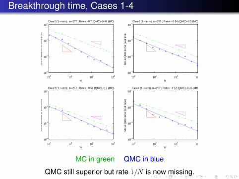
Breakthrough time, Cases 1-4
103 104 105 106
10−4
10−3
10−2
10−1
N
MC
& Q
MC
Err
or (
exit
time)
Case1 (1−norm): m=257 ; Rates:−0.7 (QMC)−0.49 (MC)
103 104 105 106
10−4
10−3
10−2
10−1
N
MC
& Q
MC
Err
or (
exit
time)
Case2 (1−norm): m=257 ; Rates:−0.54 (QMC)−0.5 (MC)
103 104 105 106
10−4
10−3
10−2
10−1
N
MC
& Q
MC
Err
or (
exit
time)
Case3 (1−norm): m=257 ; Rates:−0.58 (QMC)−0.5 (MC)
103 104 105 106
10−3
10−2
10−1
100
N
MC
& Q
MC
Err
or (
exit
time)
Case4 (1−norm): m=257 ; Rates:−0.57 (QMC)−0.45 (MC)
MC in green QMC in blue
QMC still superior but rate 1/N is now missing.
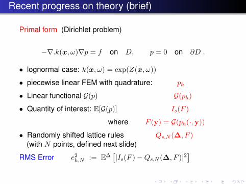
Recent progress on theory (brief)
Primal form (Dirichlet problem)
−∇.k(x, ω)∇p = f on D, p = 0 on ∂D .
• lognormal case: k(x, ω) = exp(Z(x, ω))
• piecewise linear FEM with quadrature: ph
• Linear functional G(p) G(ph)
• Quantity of interest: E[G(p)] Is(F )
where F (y) = G(ph(·,y))
• Randomly shifted lattice rules Qs,N (∆, F )(with N points, defined next slide)
RMS Error e2h,N := E∆
[|Is(F )−Qs,N (∆, F )|2
]
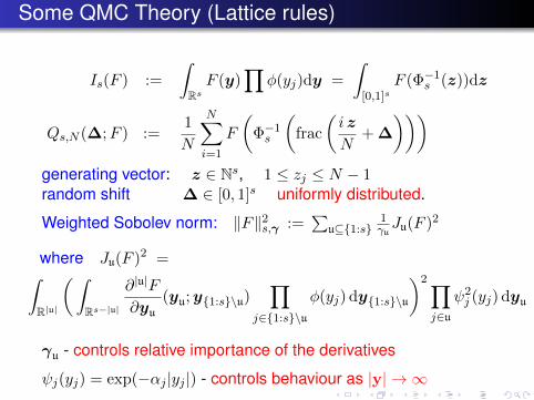
Some QMC Theory (Lattice rules)
Is(F ) :=
∫RsF (y)
∏φ(yj)dy =
∫[0,1]s
F (Φ−1s (z))dz
Qs,N (∆;F ) :=1
N
N∑i=1
F
(Φ−1s
(frac
(i z
N+ ∆
)))generating vector: z ∈ Ns, 1 ≤ zj ≤ N − 1random shift ∆ ∈ [0, 1]s uniformly distributed.
Weighted Sobolev norm: ‖F‖2s,γ :=∑
u⊆1:s1γuJu(F )2
where Ju(F )2 =∫R|u|
(∫Rs−|u|
∂|u|F
∂yu(yu;y1:s\u)
∏j∈1:s\u
φ(yj) dy1:s\u
)2∏j∈u
ψ2j (yj) dyu
γu - controls relative importance of the derivatives
ψj(yj) = exp(−αj |yj |) - controls behaviour as |y| → ∞
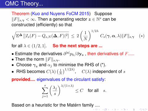
QMC Theory...
Theorem (Kuo and Nuyens FoCM 2015) Suppose‖F‖s,γ <∞. Then a generating vector z ∈ Ns can beconstructed (efficiently) so that√
E∆ [|Is(F )−Qs,N (∆, F )|2] ≤ 2
(1
N
)1/2λ
Cs(γ,α, λ)‖F‖s,γ (∗)
for all λ ∈ (1/2, 1]. So the next steps are ...
• Estimate the derivatives ∂|u|ph/∂yu , then derivatives of F .....• Then the norm ‖F‖s,γ .• Choose γu and αj to minimise the RHS of (*).• RHS becomes C(λ)
(1N
)1/(2λ), C(λ) independent of s
provided.... eigenvalues of the circulant satisfy:s∑j=1
(λjs
)λ/(1+λ)
≤ C for all s.
Based on a heuristic for the Matern family ....

Rates for the Matern class
• Dimension independent rate O(
1N−(1−δ)
)δ arbitrarily small, if
ν > 2.
• Dimension independent rate at least O(
1N
)1/2 if ν > 1
Heuristic assumes eigenvalues of the circulant approacheigenvalues of the corresponding periodic covariance integraloperator.
Conclusion:
For Matern parameter ν large enough, combined FE and QMCerror:√
E∆ [|E[G(p)]−Qs,N (∆,G(ph))|2] ≤ C[h2 +N−(1−δ)].
with δ arbitrarily close to 0 independent of dimension s.
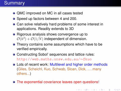
Summary
QMC improved on MC in all cases testedSpeed up factors between 4 and 200.Can solve relatively hard problems of some interest inapplications. Readily extends to 3DRigorous analysis shows convergence up toO(h2) +O(1/N) independent of dimension.Theory contains some assumptions which have to beverified empirically.Constructing Sobol’ sequences and lattice rules:http://web.maths.unsw.edu.au/∼fkuoLots of recent work: Multilevel and higher order methods(Giles, Scheichl, Kuo, Schwab, Sloan, Dick, .....manyothers...)
The exponential covariance leaves open questions!
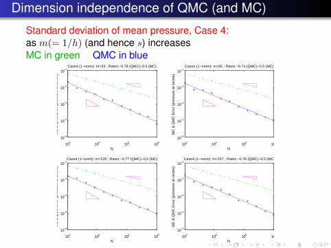
Dimension independence of QMC (and MC)
Standard deviation of mean pressure, Case 4:as m(= 1/h) (and hence s) increasesMC in green QMC in blue
103 104 105 106
10−6
10−5
10−4
10−3
10−2
N
MC
& Q
MC
Err
or (
pres
sure
at c
entr
e)
Case4 (1−norm): m=33 ; Rates:−0.78 (QMC)−0.5 (MC)
103 104 105 10
10−6
10−5
10−4
10−3
10−2
N
MC
& Q
MC
Err
or (
pres
sure
at c
entr
e)
Case4 (1−norm): m=65 ; Rates:−0.74 (QMC)−0.5 (MC)
103 104 105 106
10−6
10−5
10−4
10−3
10−2
N
MC
& Q
MC
Err
or (
pres
sure
at c
entr
e)
Case4 (1−norm): m=129 ; Rates:−0.77 (QMC)−0.5 (MC)
103 104 105 10
10−6
10−5
10−4
10−3
10−2
N
MC
& Q
MC
Err
or (
pres
sure
at c
entr
e)
Case4 (1−norm): m=257 ; Rates:−0.76 (QMC)−0.5 (MC)


