

i
University of Nairobi School of Engineering
GIS Based
Cartographic Generalization in Multi-scale Environment: Lamu County
By
Nyangweso Daniel Orongo
F56/69032/2011
A Project submitted in partial fulfillment for the Degree of Master of Science in Geographical
Informational Systems in the Department of Geospatial and Space Technology of the University of Nairobi
July 2013

i
Declaration
I, Daniel Orongo Nyangweso, hereby declare that this project is my original work. To the best of
my knowledge, the work presented here has not been presented for a degree in any other
Institution of Higher Learning.
Daniel Orongo Nyangweso 12/07/2013
Name of student Date
This project has been submitted for examination with our approval as university supervisor(s).
Mrs Tabitha Njoroge. …………………
Name of supervisor Date

ii
Dedication
I would like to dedicate this project to my wife and son.

iii
Acknowledgement
I would like to acknowledge advice accorded by my supervisor Mrs. Tabitha M. Njoroge, a
Lecturer at University of Nairobi, at the Department of Geospatial and Space Technology, which
enabled me to successfully complete the project.
I would also like to acknowledge the assistance of Mr. Charles Mwangi, a Principal Cartographer
at the Ministry of Lands, Housing and Urban Development, who assisted me in getting the
relevant data and information necessary for the project.

iv
Abstract
Generalization generally depends on the map purpose, extent of area of interest and a desired
scale. Survey of Kenya, Kenya’s National Mapping Agency, produces large amounts of different
data sets of geospatial data and at different scales. Hence there is duplication of effort, large data
storage requirement, process is slow and the data is not combined and harmonized correctly.
There is also loss of detail in the down scaling.
This paper discusses the process of vector based cartographic generalization of Lamu Vector
base data at scale of 1:5,000 using GIS software generalization tools of arcGIS 10.1 and
Quantum GIS 1.8 v. Generalization toolset. The end products were generalized maps at scales of
1:10,000, 1:50,000 and 1:100,000 produced in a fast, efficient manner to produce detailed
updated maps. The base data was contained in a file geo-database at scale of 1:5,000 was then
generalized to geo-databases at scales of 1:10,000, 1:50,000 and 1:100,000. The base data
contained feature datasets categories such as topographical, transportation, water areas,
vegetation boundaries, swamps and other special and unclassified data. General specifications
and constraints for each scale of generalization were used to symbolize the layers after
generalization. Contour and spot height data were regenerated by changing contour interval and
spot height spacing, for each scale, using Global mapper.
From the results obtained it indicates that, GIS cartographic generalization provides a good
opportunity to generalize large scale data. The process is fast and efficient and would enable one
to obtain updated detailed maps up to two times. However there is a requirement of editing and
symbolization to preserve important details. Hence there is a need to formalize on how to use
GIS software generalization techniques, to combine and harmonize data through generalization
to scales desired.
v
Table of Contents
Declaration.......................................................................................................................................i
Dedication.......................................................................................................................................ii
Acknowledgement..........................................................................................................................iii
Abstract...........................................................................................................................................iv
Table of Contents............................................................................................................................v
List of Figures and Tables............................................................................................................viii
Abbreviations................................................................................................................................xii
CHAPTER 1: INTRODUCTION ....................................................................................................1
1.1.0 Background ........................................................................................................................ 1
1.1.1 Reasons for Generalization ................................................................................................ 2
1.2 Problem statement ................................................................................................................. 5
1.3 Objectives .............................................................................................................................. 7
1.4 Justification for the study ...................................................................................................... 7
1.5 Scope ..................................................................................................................................... 7
CHAPTER 2: LITERATURE REVIEW .........................................................................................9
2.0. How little is enough ............................................................................................................. 9
2.1 Multi-Scale Mapping ........................................................................................................... 11
2.1.1 Generalization toolsets in GIS softwares ......................................................................... 11
2.1.2 Types of Generalization ................................................................................................... 12
2.2 Previous Research on Conditions for generalization ......................................................... 13
2.2.1 Data integration ................................................................................................................ 14
2.2.2 Fractal dimensionality of curves ...................................................................................... 14
2.3 The relation of data compaction rate to map scale based on Radical law ........................... 16

vi
2.3.1Testing the Radical law ..................................................................................................... 17
2.3.2 Factors or Indicators which govern Generalization ......................................................... 17
2.4 Quality evaluation ............................................................................................................... 20
CHAPTER 3: METHODOLOGY ................................................................................................26
3.1.0 Measuring equipment and Materials used in Collecting Base data for Generalization ... 26
3.1.1 Source of Geospatial data ................................................................................................. 26
3.1.2 Softwares and Hardware .................................................................................................. 26
3.1.3 Data preparation and matching ........................................................................................ 31
3.1.2 Creation of Grid Layers .................................................................................................... 31
3.1.5 Data identification ............................................................................................................ 33
3.1.6 Visualization of building layer at different scales ............................................................ 36
3.2 Methodology used in Cartographic Generalization ........................................................... 39
3.2.1 Generalization Toolsets overview .................................................................................... 40
3.2.2 Overview of the generalization toolset in ArcGIS 10 and Qgis 1.8 softwares ................ 40
3.2.3 Cartographic Generalization of Base data at scale 1:5,000 .............................................. 44
3.2.4 Buildings Generalization .................................................................................................. 45
3.2.5 Shoreline simplification ................................................................................................... 45
3.2.6 Roads Generalization ....................................................................................................... 46
3.2.7 Contour Generalization .................................................................................................... 46
3.2.8 Spot height Generalization ............................................................................................... 47
CHAPTER 4: RESULTS AND DISCUSSIONS ..........................................................................49
4.0 Vector Feature Generalization Results ................................................................................ 49
4.1 Building Generalization Results .......................................................................................... 49
4.2 Building Generalization at 1:100,000 scale by aggregation at 20 metres ........................... 52

vii
4.3 Road Generalization details ................................................................................................ 55
4.4 Contour Generalization Results .......................................................................................... 59
4.5 Spot height Generalization results ....................................................................................... 62
4.6 Shoreline Generalization details .......................................................................................... 63
4.7 Quality assurance and control on cartographic generalization ............................................ 65
4.8 Challenges encountered in Cartographic Generalization .................................................... 66
CHAPTER 5: CONCLUSION AND RECOMMENDATIONS ...................................................67
5.1 Conclusion ........................................................................................................................... 67
5.2 Recommendations ............................................................................................................... 67
REFERENCES ..............................................................................................................................68
APPENDICES ...............................................................................................................................75
Appendix A1 Map clip at Base scale level 1:5,000 .................................................................. 76
Appendix A2: Generalized map clip at scale level 1:10,000 .................................................... 77
Appendix A3: Generalized map clip at scale level 1:50,000 .................................................... 78
Appendix A4: Generalized map clip at scale level 1:100,000 .................................................. 79
Appendix B1 Symbols table scale 1:5,000 (base scale) ............................................................ 80
Appendix B2 :Symbols table scale 1:10,000 ............................................................................ 81
Appendix B3: Symbols table scale 1:50,000 ............................................................................ 82
Appendix B4: Symbols table scale 1:100,000 .......................................................................... 83
viii
List of Figures and Tables
List of Figures
1 Figure 1: Generalization concept .................................................................................................5
2 Figure: 2 Generalization model by Gruenreich ...........................................................................9
3 Figure: 3 The generalization process .........................................................................................10
4 Figure: 4 Importance of cartographic generalization operators .................................................10
5 Figure 5: Categories of design change while generalizing ........................................................18
6 Figure 6: Cartographic Model Construct approaches of features ..............................................19
7 Figure 7: Most Problematic cartographic generalization operators ...........................................21
8 Figure 8: Map of Lamu County showing area of interest bounded in a rectangle .....................28
9 Figure:9 Lamu Grid map layers with inset of County Maps showing area of interest ..............29
10 Figure 10: Grid layer creation for Scale 1:10,000 using ArcGIS create fishnet tool ...............32
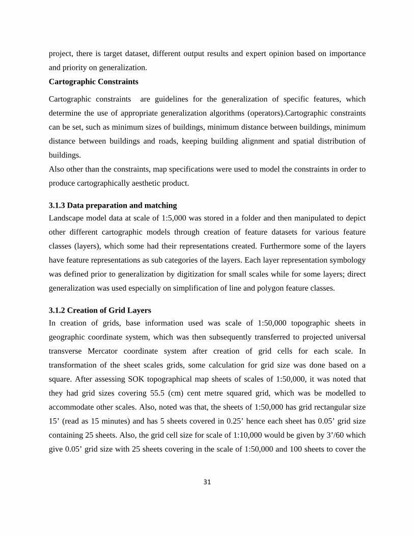
11 Figure 11: Base data used in Generalization ............................................................................33
12 Figure 12: Scale Settings .........................................................................................................34
13 Figure 13.Visualization of Lamu buildings 1:2,500 ...............................................................35
14 Figure 14.Visualization of Lamu buildings 1:5,000 scale .......................................................35
15 Figure 15:Visualization of Lamu buildings 1:10,000 scale ..................................................35
16 Figure 16: Visualization of Lamu buildings 1:50,000 scale .................................................36
17 Figure 17: Visualization of Lamu buildings 1:100,000 scale ...............................................36
18 Figure 18a: Grid layers on a fixed paper size on various scales ..............................................36
18 Figure 18b: Grid layers on a fixed paper size on 1:5,000 ........................................................37
19 Figure 19: Methodology used ..................................................................................................38
20 Figure 20: Some of the generalization tool in ArcGIS Software .............................................39
21 Figure 21: Lamu DEM used in generating spot heights and Contours ....................................45
22 Figure 22: v. generalized algorithm generalization script .......................................................47
ix
23 Figure 23: Location Diagram and Index to adjoining sheets ...................................................48
24 Figure 24: Building aggregation at 5metres .............................................................................49
25 Figure 25: Building Simplify at 10 metres ..............................................................................49
26 Figure 26: Building conversion to point using Polygon to point conversion tool ...................50
27 Figure 27: Building point generalization .................................................................................50
28 Figure 28: Buildings at scale 1:100000 before generalization .................................................51
29 Figure 29: Buildings at scale of 1:100,000 after generalization ..............................................51
30 Figure 30: Delineating Builtup areas using 20 metres as tolerance .........................................52
31 Figure 31: Delineating Builtup areas using 50 metres as tolerance .........................................53
32 Figure 32: Superimposing the layers after aggregation ...........................................................53
33 Figure 33: Building generalization by use of delineate builtup area tool ................................54
34 Figure 34: Roads Generalization process success dialog ........................................................54
35 Figure 35: v. generalized algorithm, network method in Q-Gis ..............................................55
36 Figure 36: Before applying Collapse Dual Line to centreline tool (zoom 1:250k) ................56
37 Figure 37: After applying Collapse Dual Line to centreline tool(zoom:1:250k) ....................56
38 Figure 38: After generalization ................................................................................................56
39 Figure 39: Before generalization .............................................................................................56
40 Figure 40: Collapse of dual roads to centreline overlay with initial data ................................57
41 Figure 41: Road Generalization at Scale 1:50,000 and 1:100,000 ..........................................57
42 Figure 42: Generalized map with all the layers generalized at the scale of 1:100,000 ............58
43 Figure 43: Contour Generation for smaller scales using general specifications ......................59
44 Figure 44: Contour Generalized using Imhof (2007) and Frye (2008) specifications .............60
45 Figure 45: Spot Height generalization .....................................................................................59
46 Figure 46: Shoreline simplifications for various scales ...........................................................63

x
47 Figure 47: Generalized maps clips ...........................................................................................64

xi
List of Tables
1 Table 1: Selection of contour intervals as per scale ...................................................................24
2 Table 2: Scales and grid cell size in metres for designing of map layout plans ........................33
3 Table 3: Arc-Gis 10.1 tools in the generalization toolset ..........................................................40
4 Table 4: Building simplification constraints used .....................................................................44
5 Table: 5 Shoreline line simplification by Bendsimplify and point remove ...............................45

xii
ABBREVIATIONS
AAI Applied Artificial Intelligence
AOI Area of Interest
CAC Coefficient of Area Correspondence
CLC Coefficient of Line Correspondence
CLIPS C Language Integrated Production System
EuroSDR European Spatial Data Research
ESRI Environmental Systems Research Institute
GIS Geographic Information Systems
GPS Global Positioning Systems
ICA International Cartographic Association
ITC International Training Centre
KLR Kenya Law Reporting
LiDAR Light Detection And Ranging
MRDB Multi Resolution DataBase
MAS Muilt Agent System
NMA National Mapping Agency
UTM Universal Transverse Mercator
SoK Survey of Kenya

i
CHAPTER 1: INTRODUCTION
1.1.0 Background The current world of map making is production of geospatial information at various scales as
demanded by users ranging from general public to government sectors and from commercial
industrial applications to scientific research. Hence, to meet the needs and to shorten up data
cycles of the derived maps, National Mapping Agencies (NMAs) are considering use of fast
generalization process. The generalized maps should be such that, they can be used as paper
maps, or relayed via displays such as web browsers through web portals or handheld mobile
devises. Generalization is defined as the process of meaningfully abstracting the infinite
complexity and diversity found in the real world into a single, targeted cartographic
representation and that is usable and useful for the given map scale and purpose, (Muller and
Wang, 1992). Data layers should be maintained; displayed, arranged for ease of access and even
how layers are allocated names should be conveying meaning. Potential generalization solutions
are needed to customize the resulting maps for a specific theme and purpose and hence a
cartographer with these requirements is needed to ensure that the map is an appropriate
representation of the portrayed geographic information. The process of generalization occurs
such that some geographic details are emphasized at the expense of others.
According to the Survey Act, Cap 299 Laws of Kenya (KLR 2010) Survey of Kenya (SoK) is the
National Mapping Agency (NMA). Its mandate is the preparation of the national Base map. SoK
produces geospatial data at various scales to satisfy diverse needs of citizenry. Furthermore, SoK
is mandated to define features on a topographical map, which are governed by their presence on
the ground and are mapped within the limits of scale. In carrying out the above responsibilities,
standards are required to govern or regulate process of surveying and mapping for quality control
through the Kenya survey manual which is yet to be revised as it is dated 1962.
The demand of producing maps automatically has since increased and aided by continuous
evolution of GIS since 20th century and increased availability of automated generalization tools
and methods used by National Mapping Agencies (NMAs) and other geospatial data providers.
Map contents should be reduced to what is necessary and possible by emphasizing what is
important while repressing less important contents. The paper uses the available generalization
2
tools in the Computer GIS softwares with minimal manual cartographic editing. There is
interaction between omitting and repressing while, exaggerating and emphasizing on the other. It
accompanies all the construction stages of the map, from the conception design to the final
reproduction. Most important is good communication of all measures with a view to producing
details of the possible consistency.
Generalization starts where self evidence of the graphic statement and legibility become
insufficient. What is required of generalization includes but not limited to the following:
• Positional accuracy depending on scale
• Accuracy of forms of lines within the limitations of scale
• Hydrographical alignments in relation to other linear features like coastlines.
• Simplification of forms of lines corresponding to the generalized terrain forms
• Relationship of the hydrographical networks to the other map elements and there is a
theoretical requirement for maps that the black to white ratio at all scales should remain
constant
In designing cartographic maps consider that:-
a. No new data is generated.
b. Adopt simple geometric symbols; no missing layers or text on export
c. Commonly used fonts for export and file sharing which are legible
d. List of group layers to easily turn off categories while evaluating appearance
e. Attention to symbol levels and maplex weights (software tool) as found in GIS
softwares.
f. All rasters and layers with transparency at bottom of table of contents (GIS layers), so
that on export it retains editable vectors and type.
g. No over/under passing on corridors and colour ramps
(Source: Stoter, 2005).
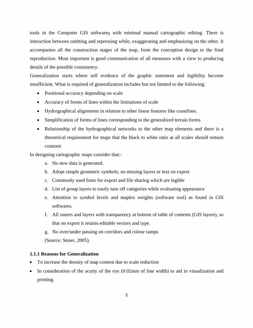
1.1.1 Reasons for Generalization • To increase the density of map content due to scale reduction
• In consideration of the acuity of the eye (0.02mm of line width) to aid in visualization and
printing.

3
• To preserve minimum sizes of known objects while keeping important obvious objects,
differences in form to be clear, improve illumination and light printing to increase contrast
and to avoid blurred reproduction since no precise production and print technique available
or for economical purposes.
For example minimum sizes for scale of 1:50,000 are:-
To start with cartographic symbolization, sizes are symbolization layer properties which define
point, line or polygon shapefile sizes, but should not be taken to be a measure of metric or
empirical units. The sizes determine how layer’s size is depicted as a representation. Some take
width size while others especially point symbols take size with a variable ranging from 0 to 100.
Roads: for divided roads Tarmac line size of 0.2 at the edges with width of line size of 1.1
Earth road (class 1) line size 0.22 at edges and width 0.75, and the class 2 (motor able track) and
class 3 (foot Path and others) both having edge size of 0.12 widths of 0.6 and 0.5 respectively
Points: points drawn with font size 0.75 with triangular points’ side 1.0 as length
Point labels: font size of 0.7.
Contours: Contours: index contour line size 0.18, normal 0.09-0.10 (10 metre contour interval),
supplementary lines drawn as dashed among others. (Source: Publication of Swiss Society of
Cartography, Publication number 2)
The above minimum sizes are defined in map specification, for every scale of interest.
Based on constraints and decreasing number of objects as compared to the ground we have that;
on a 1:50,000 scale, side length and area on ground can vary for each scale or in change of
geometry and decreasing number of objects as explained by the Swiss society of cartography,
publication number 2.
Factors which influence cartographic generalization
• Scale.
• Source material.
• Choice of colours.
• Technical reproduction capabilities.
• Revision updates.

4
Assumption for Map Generalization
Assumptions for geospatial data generalization are that, data points may take any position in the
Euclidian plane and their location after generalization are assumed to be scale free.
Map generalization at different scales traditionally relies on different datasets at different scales.
Generalization can be partly assembled, (Stoter, 2005), from software codes, written map
specifications and one carried out by cartographer using various operations. Generalization
operators, as stated by Mark Denil (2011) are defined as an abstract or generic representation
describing the type of modification that can be used when generalizing while an algorithm is a
particular implementation of the operator, (Regnauld and McMaster, 2007). Examples of
algorithms in the cartographic practice include the Douglas-Peucker algorithm, (Douglas and
Peucker, 1973), the Walking algorithm, (Müller, 1987), ATM filtering, (Heller, 1990),
optimization simplification, (Cromley and Campbell, 1992), the Visvalingham- Whyatt
algorithm, (Visvalingham and Whyatt, 1991), and the modified Visvalingham-Wyatt algorithm,
(Zhou and Jones, 2004); (Bloch and Harrower, 2006), among many others.
After generalization, the cartographer’s objective is to communicate the information present in
the map produced as simply as possible. This presentation of information can be done through
visualizing in vector mode and / or raster mode generalization. Visualizing in vector mode as
stated by McMaster(1992) is by simplification, smoothing, aggregation, amalgamation, merge,
collapse, refinement, typification, exaggeration, enhancement and displacement and the vector
operators relate to those by Roth, R., Brewer, C., Stryker, M.(2012). In the case of amalgamation
a series of lakes, Islands or closely related forest stands are fused together. In aggregation a
series of point features are fused into areal feature represented by an enclosing boundary.
Smoothing can be applied to contour and polygon features can be used to display both
displacement as with simplification using displacement vectors and area and changes in the
angularity and curvilinearlity of a given feature.
Likewise, visualizing in raster mode generalization includes such models as those of McMaster
and MonMonier (1989) whereby raster mode generalization operators used are structural,
numerical, numerical categorization and categorical generalization. In, addition, generalization
operators are either geometric or semantic. Geometric operators are for reduction in number of

5
discrete features (by geometric selection), reduction in detail of individual line, areal and surface
features (reduction in sinuosity) and amalgamation of neighbouring features, whether point, line
or area. Vector mode generalization is the area of research and its applications are discussed in
detail. Aerial raster images captured were used for semantic discerning of features in the area of
interest (AOI).
1.2 Problem statement
Currently, SoK is in the process of revising specifications and procedures of map making.
National Mapping Agencies like SoK annually produce enormous amounts of geospatial data;
geodetic, aerial and manual data entry and scans of analogue data. This data is produced from
different sources and is used to produce a variety of different map products at different scales. In
most cases, the data is public; in particular the topographical maps and administrative boundary
maps. Disseminating data to the public is sometimes slow and sometimes makes the clients or
customers to acquire both necessary and unnecessary data. Hence, it would be convenient for
SoK to adopt a system where clients obtains data of the area of interest (AOI) only, at large
scale, which would enable one to have as much detail for AOI.
In Kenya most topographical and thematic maps (common products produced by SoK) are at the
scales of 1:50,000 and 1:100,000 and towns are mapped at scales of 1:10,000 as topocadastral
maps. Other topographic maps include those of scale 1:250,000 for regional parts of Kenya and
1,000,000 which cover the entire country. Hence to represent data for the whole country needs
some generalization for representation in small scale maps containing details which are up to
date, through formalized procedures.
Generalization of Geospatial Data
A concept of generalization like that of McMaster and Shea, (1998) can be used to determine
why when and how in generalization of geospatial data.
Why when how
Figure 1: Generalization concept McMaster and Shea, (1988).
Philosophical Objective Theoretical elements Application specification elements Computational elements
Cartometric evaluation Geometric Conditions Spatial and holistic measures Transformation control
Geometric and attribute transformation Graphic and Conceptual Generalization

6
A grid layer box of varying area of extent using the same paper size is used to define number of
feature to be retained. If the same paper size is used of varying extents (as defined by grids) then
features will be competing for space from one scale transition to another.
Operations in map production at the mapping agency, for example, are that, maps are produced
commonly in A1 size paper for topographical maps and a few on A0 size for wide extents like
thematic maps; like route maps or tourist maps. Basic maps at largest scales are normally
constructed at 1:2,500. Derived maps result often after generalization from this large scale.
The area of interest for the study is Lamu. In Lamu town, there are areas with high data density,
while others are devoid of usable geospatial data. Hence, the issue is to get a map that is
satisfactory and most economical to all stakeholders. Although, data availability for Lamu area is
one of the driving force for the research project, the same procedures and operations can be
carried out in all areas in Kenya, specifically for National topographical maps. Currently there
are new data frameworks aided by systems such as continuous observation systems enabling the
production of detailed and accurate ground survey observation being created with reference
system and new control points for production of maps. Most importantly is that in design of the
large scale and derived maps there is need for:-
i. Procedures;
ii. A single product library accessible by diverse users and for different scale abstractions
from a single geospatial data server; and
iii. Production of different versions using a single dataset.
In some cases, there would be a need to convert analogue data to digital data. This is done by use
of softwares which have capabilities as defined by licence types of software. Deliverables at the
end of project research are a sample map showing an area of the same extent shown in different
scales of generalization, with features depictions as extracted by generalization algorithms.
Hence, when a topographical map is ordered as topographical sheet number, it will be convenient
when a client defines AOI only, hence one cannot be inconvenienced in getting unnecessary data
to ascertain his AOI mapped in detail while area of no interest is highly generalized.
7
1.3 Objectives
Main Objective To generalize Geospatial data at various scales for the Lamu area using the lowest level of
detail at 1:5,000 scale to smaller scales of 1:10,000, 1:50,000 and 1:100,000 using GIS
generalization toolsets.
Specific objectives
1) To prepare a geo-database to be used to visualize the generalized data.
2) To demonstrate the use of generalization techniques for detail extraction at user specific
area.
3) Carry out modelling for the area of study.
1.4 Justification for the study
The research study is aimed at formalizing the procedures and GIS techniques, which may be
used by the NMA, SoK to generalize data from large scale to small scale using the same base
data aided by generalization algorithms incorporated in GIS softwares and together with use of
human visual mind to create cartographically sound maps at small scales. The benefits of
formalizing the generalization procedures for the scale of 1:10,000, 1:50,000 and 1:100,000
include:-
a) Efficient and faster updating of existing small scale map at SoK
b) Request for maps based on a scale specification and area of interest.
c) It will be easier to determine the number of sheets required based on the AOI at the scale
desired by clients.
d) Specialised workflows and rules integration for each dataset.
e) There will be fewer databases as data is centric.
1.5 Scope
The scope involves generating maps at various scales using generalization rules and tools in
arcGIS 10 and QuantumGIS 1.8 softwares. In addition, there would be minimal digitization of
some features, creation of representations of generalized data and storing the results in a geo
database. Area of interest will be modelled to contain grid layers partitioned for sheets of maps
8
covering scales of 1:5,000, 1:10,000, 1:50,000 and 1:100,000. Generalization of geospatial data
at the base scale of 1:5,000 will be carried out using generalization toolset found in GIS software
such as simplification, smoothing, aggregation, collapsing and thinning road network among
others.
Spot heights and contours will be regenerated using Global Mapper software. The generalized
data would then be represented on map sheets as defined by the grid layers. Symbolization and
editing of the data will be carried out and size of some symbols for data for generalized maps
would be kept constant for generalization scales as data to represent on them covers the same
area for ease of comparison. Finally, process control and quality assurance of the generalization
would be done using cartographic visualizations on screen or in prints to ascertain the use of
symbolization, constraints of minimum sizes as contained in specification standards. Also, within
the software, quality of process will be evaluated using statics summary and contents summary
and through use of appropriate tolerance parameters for input operators.
The area of study was part of Lamu county, with area represented by four topographical map
sheets at the scales 1:50,000 which cover an area of one sheet of scale 1:100,000. Generalization
was carried out on base vector data at scale of 1:5,000 and generalised to scales of 1: 10,000,
1:50,000 and 1:100,000. Concentration on generalization was for clear and effective cartographic
visualization using vector data only.
Report Organization
The report contains five chapters covering introduction, literature review, methodology, results
and discussion and conclusions and recommendations. References and appendices pages are
included at the end.

9
CHAPTER 2: LITERATURE REVIEW
2.0. How little is enough The question of addressing how little is enough, will be addressed by presenting initial results to
showcase a significant relationship between generalization scales and usability of the
corresponding maps as consistently transmitted. In some cases, some data may be poorly
represented and consequently a poor representation of the feature is depicted. In addition, smaller
data sizes, a quick response times and possibility of transmission of only relevant details is
possible, (Bertolotto, 2007) as stated in Fangli Ying et al (2011). For maps containing many
polygons and lines, a methodology for determining a globally suitable generalization is
necessary. There is also a need to associate the generalized data with quality information with
additional derived representations.
Graphic representations of lines for scales of 1:50,000 and 1:100,000 (0.15mm) and minimum
sizes of 3mm for (1:50,000 and 1:100,000) and areas of map symbols covering ground distances
of 15m side length and 30m and sizes as those of Swiss Society of Cartography by Alfred
Rytz(1987) can be used.
Figure 2: Generalization model by Gruenreich (1992) as adopted by Forster et al (2007)
10
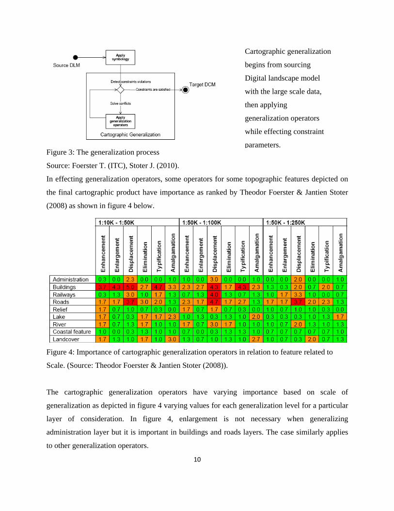
Figure 3: The generalization process
Source: Foerster T. (ITC), Stoter J. (2010).
In effecting generalization operators, some operators for some topographic features depicted on
the final cartographic product have importance as ranked by Theodor Foerster & Jantien Stoter
(2008) as shown in figure 4 below.
Figure 4: Importance of cartographic generalization operators in relation to feature related to
Scale. (Source: Theodor Foerster & Jantien Stoter (2008)).
The cartographic generalization operators have varying importance based on scale of
generalization as depicted in figure 4 varying values for each generalization level for a particular
layer of consideration. In figure 4, enlargement is not necessary when generalizing
administration layer but it is important in buildings and roads layers. The case similarly applies
to other generalization operators.
Cartographic generalization
begins from sourcing
Digital landscape model
with the large scale data,
then applying
generalization operators
while effecting constraint
parameters.

11
2.1 Multi-Scale Mapping Multi-scale mapping is where each individual layer is generalized for use at a particular range
(minimum and maximum range of displays). Multi-relational database (MRDB), offers, for
multi-scale mapping, a technical solution for automating map design process, to bring a higher
integration of geographic data and map design, easier map updates and a more consistent
cartographic design across scales and hence enable the public to view using web mapping
services, Roth and Rose (2009) beyond the “one map” solution Monmonier, (1991) as mentioned
by Mark Denil (2011). In other areas like open street map and Google maps, one can edit styles
across scales hence the question of the degree at which multi-scale mapping choices should be
constrained by expert knowledge varies due to cartographic democracy (Wallace, 2010). Hence
from the above, multiscale mapping is related to NMA, web map service and multiscale
representation databases.
In Multi-scale mapping, operators are based on content, geometry, symbol and label. Multiscale
mapping describes the cartographic practice of generating integrated designs of the same
geographic extent at multiple (or all) cartographic scales. Multiscale mapping and generalization
are not the same. Generalizations describes the design decisions made for a single scale, with
goal of reducing detail as scale is fixed Brewer and Buttenfield (2010). MRDB links several
geographic entity across scale, resolutions, purposes Kilpelainen (1997); Sarjakoski (2007).
Research on GIS and automated generalization and conceptual models is documented by
Gruenreich, Brassel and Weibel and McMaster and Shea, (2005) models. In the models, there are
various views on automated generalization: the representation-oriented view and the process
oriented view. In the representation view, focus is on the representation of data at different
scales, related to multi-representation database (MRDB). The process view focus is on process of
generalization. In creation of databases at different scales, there is a difference between the
ladder and star approach. The ladder approach is the case where each derived dataset is based on
other database of the next larger scale. The star approach is the derived data at all scales and
relies on a single (large-scale) database.
2.1.1 Generalization toolsets in GIS softwares ArcGIS Generalization toolset include tools enabling simplification or refining features for
display at smaller scales. The tools include aggregate points, aggregate polygons, collapse dual
12
line to centreline, delineate built-up areas, reduce road detail, merge divided roads, simplify
building, simplify line, simplify polygon, smooth line, smooth polygon and thin road network
(ESRI ArcGIS online resource 2012). Open source softwares like QuantumGIS (QGIS) 1.8 have
generalization tools. Each of the software has tools suited for specific situations and feature
classes work best in terms of types of features class. For example, in the collapse dual lines to
centreline tool, the tool derive centreline from dual line (or double line) features, such as road
casings, based on specific width tolerances. It is used for regular, near parallel pairs of lines, such
as large scale road casings.
Centrelines can be created only between open ended lines and not inside closed lines which are
likely street blocks. The tool further is not intended to simplify multiple lane highways with
interchanges, ramps, overpasses and underpasses, or railways with multiple merging tracks.
Merge divide tool is used instead. The topic of generalization is a research topic for EuroSDR for
the year 2011 and 2014, titled, “Semantic interoperability: Ontology, schema translation, and
data integration”.
2.1.2 Types of Generalization Generalization can be model or cartographic based. Cartographic generalization involves
enhancement, displacement, elimination, typification, enlargement and amalgamation while
model generalization is concerned with class selection, reclassification, collapse, combination,
simplification and amalgamation. Model generalization, multi-resolution and multi-
representation data bases was Topic no. 9, titled, “Cartographic generalization in terms of up-
and downscaling, for traditional and non-traditional displays”, Euros(2012), (www.eurosdr.net)
for the year 2012. 3D (three dimensional) generalization becomes an issue, especially when
using more mobile (handheld) computing devices like an iPhone. Cartographic generalization
was topic no. 11. of International Cartography Association(ICA) Commission on Map
Generalization and Multiple Representation and European Spatial Data Research (EuroSDR)
Commission 4 on "Data Specifications", a 15th organized workshop which was held on
generalization, at Istanbul, Turkey, on 13-14 September, 2012.
When designing multiple scale representation, one has to consider linking existing datasets of
different scales or thematic representation by a specified matching procedure. This is then

13
followed by creation of new data sets from existing ones, creating new layer of a different scale
in the representation.
Dulgheru (2011), in his international conference scientific paper, he examined generalization
tools or algorithms for map generalization with ArcGIS software. Other commands like
bendsimplify operator in house algorithm, orthogonal operator and building simplify,
findconflicts, centerline, area aggregate and generalize command. However, the tools introduce
labelling and topology errors if error check is not specified. Error check is iterative and if
topological errors are present, arcs involved will be re-generalized using a reduced tolerance.
Further, other commands like build command are used to obtain polygon topology so as to avoid
label and silver polygons. Line simplification using Douglas Peucker algorithm is used mostly
due to its cartographic soundness as evaluated by Visvalingam, M and Whyatt, J D (1991). The
generalization tools are utilized to produce a cartographically generalized map outputs.
2.2 Previous Research on Conditions for generalization In evaluation of map detail, some of the analytical laws are used in applying in number of objects
with scale of map change like Topfer’s Radical Law have been existing, Topfer and Pillewizer,
(1966).
Cases where there are rules governing generalization are referred to as, rule based generalization
and one on free based generalization, whereby there are no rules, every cartographer designs on
what to include and exclude based on map purpose. Free based generalization was common in
traditional cartography but the rule based one is currently used in a computer and information
environment. Research by Topfer is based on such rules, and is what is called empirical radical
law on generalization and is given by the equation
FAAF MMNN /= ……………………………………………………………………….(2.2.1)
Where
FN = is the number of objects which can be shown at the derived scale,
AN = is the number of objects shown on the source material, AM = is the scale denominator of the source map, and
FM = is the scale denominator of the derived map. ( Topfer and Pillewizer, 1966)

14
Topfer further generalized the equation by including a constant, where he specified that a value
of 1 applies to point symbols and 2 areal symbols among others. However, the Radical law has
limitations, since it does not indicate the objects to be selected and there is no consideration of
local variation in the density of phenomena, (Jones. C, 1998).
2.2.1 Data integration In data integration, dataset should match geometrically and topographically, that is, have same
spatial relationship in the data as those in the real world, and have a correspondence of attributes,
Usery, L (2009). According to Usery’s analysis, if linear ratio of scale denominator are >=0.5,
then integration is possible through mathematical transformations and adjustments. He further
stated that ratios <0.5, generalization results will be incompatible differences= 0.25 where data
integration cannot be achieved hence requires manual / interactive adjustment of spatial data
elements whereby these kind of results have in themselves the meaning for a limited application.
He further concluded that, if scale denominators of source map for vector data are within a factor
of two, then the datasets can be integrated. If the factor is greater than two, then it may be
impossible to integrate the datasets. In this case significant processing and human intervention is
needed to add value to such data.
2.2.2 Fractal dimensionality of curves Additional research has been done on fractural dimensionality of point and line curves. The line
curves are used to predict, during generalization, the maximum number of describing points for a
given map scale, while assuming statistical self similarity for the geographic line.
Co-ordinate compaction rate
Map scale reduction can be done for scale independent databases assuming that data points for
small scale representations are always a subset of large scale representations.
Linear relationship
Previous research by Usery showed that coordinates compaction rates depend on the
generalization algorithm being used, the fractal dimension of the line and the map scale
reduction. Other cases, Muller (1987) compares generalization algorithms of moving average,
Douglas Peucker, walking, for the shading among others published in early years when issue of

15
generalization arose; requires urgency of formalizing the process of cartographic generalization
so that it can be automated , Jenks, (1979); McMaster, (1983); White (1985).
Concept of fractal dimension may be used to predict the maximum number of describing point
for a given map scale assuming statistical self similarity for the geographic line. Assuming point
selected for small scale represented is a subject of the scale representations. The point or distance
travelled / traversed generalization algorithm can be a subset of the original point. Otherwise the
walking generalization algorithm can be of use for applying the minimum separation rule
(Muller, 1987), new sequence of points which are equally distant from each other. Total number
of describing points can be predicted. The concept of fractal dimension can be used to calculate
the number. Assuming the line digitized is a fractal that is, every shape is geometrically similar
to the whole, the property is called self similarity, Maundelbrot (1982). According to Richardson
(1988), and Richardson (1961) equations in Muller J (1987).
L(�)=� ** (1-
D)………………………………………………………………………………..(2.2.2)
Where
� is the step length of the line L(�) and D is a constant let N= number of steps � used to
measure the line length.
Then L(�)=N× � From equation 2.2.1 above N× � = � ** (1-D) 1nN+1n �= (1-D) 1n � 1 nN/1n �=-D Or D=1 Nn/ln(1/ �)……………………………………………………………………………(2.2.3) D is called the fractal dimension where,
1/ � =number of steps of length –partitioning the base line (a straight line joining the first and
the last point of the curves basic fractal generator which in the case of geographic line, is the
whole line used. Hence equation 2.2.1 can be stated as,
D=1-1nL(�)/1n(�)……………………………………………………………………….…(2.2.4)
Further it can be stated that, the geographic line is said to be statistically self similar when the
relationship between 1nL and Ln(� )is linear . For this case, the limit that
16
(1Nl (� + �)-1Nl(�))/ �
Where � ->0, is estimated through regression analysis and is used to determine the fractal
dimension in equation 2.2.4. Hence, when the fractal dimension of a given geographic line is
available, then the value of N can be determined as:
1nN=Dx1n (1/ �) Or N=� ** 1N91/ �)xD………………………………………………………………………(2.3.5) The steps of length � are the strokes of the curve, and according to the minimum separation rule,
these may not be smaller than , of the points forming the curve.
Furthermore, some complex lines with narrow spikes and wide may make self intersection-
colliding by themselves, which also happens when using Douglas Peucker algorithm (1973) as
reviewed by Muller (1987). In most cases, cartographers attempt to solve this problem by
identifying colliding points and displace them. Currently, this is still a research area.
The problem of spikes has previously been dealt with, ( Deveau 1985). Limitation of the fractal
curve measurements is that, not all points lie in a straight line as any other may fall between two
points and hence is a redundant as per standards of minimum separation rule. Also, N can be
predicted for self similar lines only. In addition, earlier research has indicated that geographic
lines are not always self similar, (Hakanson (1978); Goodchild (1980) as shown in Muller
(1987).
2.3 The relation of data compaction rate to map scale based on Radical law Radical law, or principle of selection provided by Topfer and Pillewizer(1966) describe a line such that, NxM=Constant
Where
N=number of points describing the line.
M= denominator of map scale.
The law asserts that there is a hierarchy in method of line storage as number of points retrieved is
related directly to the scale of the required map, as reflected in Jones and Abraham, (1986) but
this is not usually always the case (Jones and Abraham 1986).
17
2.3.1Testing the Radical law Radical law was tested by Usery L. ( 2009), where he used moving average, walking and
Douglas Peucker algorithms to represent the line at different scales while generalizing according
to the scale reduction rates. The results of the Douglas Peucker gave worst result as compared
with the others. However, the Radical law is applicable to simpler lines but not with complex
lines. The relation between data compaction and scale reduction is a function which depends on
line complexity and method of generalization. In the case of statistically self similar geographic
lines, one can include effect of complexity by using the relation that,
N1=No ((Mo/Mi) **D
Where
D=Fractal dimension of the line
No and N1 are number of describing points on the larger and smaller scale maps respectively.
Mo and M1 are the corresponding scale denominators
While for space filling curves, the reduction in the number of describing points would
correspond to the reduction in the map area.
N1=No [(Mo/M1) **2] ……………………………………………………………….. (2.3.6)
Successive application of the relation depends on the appropriate point density on the original
source map.
Furthermore, one should use the minimum separation rule in NxM=constant, that
1= 0(M1/M0) **D
Where
0 and 1 are the minimum spacing between the describing points on the original map and the
new derived map after generalization, (Muller J.C, 1987).
2.3.2 Factors or Indicators which govern Generalization Factors or indicators which govern generalization (Stuart and McMaster, 1988), outlines
conditions such as congestion, coalescence (touching each other due to small distance or
symbolization process), conflict(especially with background), complication(ambiguity relating to
complexity of spatial data, identification of iteration technique and tolerance levels to be adopted
in generalization), inconsistency(due to non uniform application of generalization process) and
imperceptibility due to loss of feature –after falling below a minimal portrayal size in a map; by

18
deletion or combination of a group of features into a single point, Labour (1986). The conditions
are to be checked as benchmarks after generalization to ascertain whether the exercise has met
the conditions so stated.
19
The generalizing process effects a variety of changes to original data and range from changes in
content, geometry, symbols or labels as elaborated in figure 5.
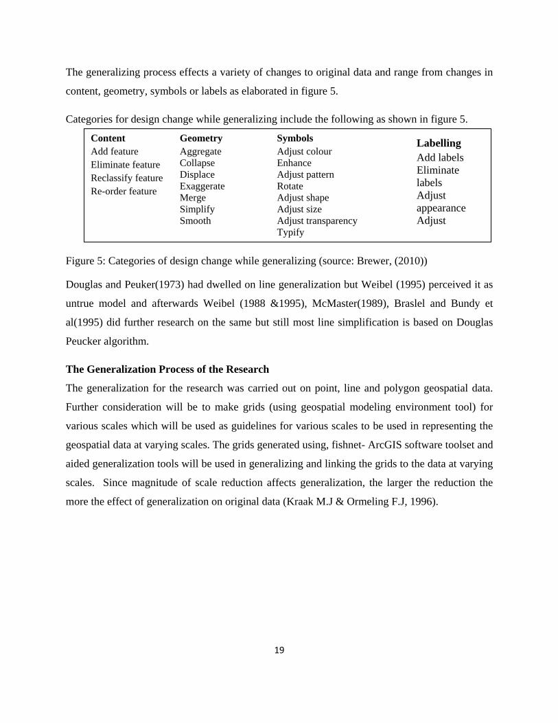
Categories for design change while generalizing include the following as shown in figure 5.
Figure 5: Categories of design change while generalizing (source: Brewer, (2010))
Douglas and Peuker(1973) had dwelled on line generalization but Weibel (1995) perceived it as
untrue model and afterwards Weibel (1988 &1995), McMaster(1989), Braslel and Bundy et
al(1995) did further research on the same but still most line simplification is based on Douglas
Peucker algorithm.
The Generalization Process of the Research
The generalization for the research was carried out on point, line and polygon geospatial data.
Further consideration will be to make grids (using geospatial modeling environment tool) for
various scales which will be used as guidelines for various scales to be used in representing the
geospatial data at varying scales. The grids generated using, fishnet- ArcGIS software toolset and
aided generalization tools will be used in generalizing and linking the grids to the data at varying
scales. Since magnitude of scale reduction affects generalization, the larger the reduction the
more the effect of generalization on original data (Kraak M.J & Ormeling F.J, 1996).
Content Add feature Eliminate feature Reclassify feature Re-order feature
Geometry Aggregate Collapse Displace Exaggerate Merge Simplify Smooth
Symbols Adjust colour Enhance Adjust pattern Rotate Adjust shape Adjust size Adjust transparency Typify
Labelling Add labels Eliminate labels Adjust appearance Adjust
i

20
Base data
Figure 6: Cartographic Model Construct approaches of features of cartographic representation
In graphic generalization operations such as simplification, enlargement, displacement, merging
and selection are used. Conceptual generalization includes merging, simplification,
symbolization and enhancement (exaggeration) (Kraak M.J & Ormeling F.J., 1996).
2.4 Quality evaluation Quality evaluation deals with examining and checking that ‘desired’ characteristics of a system
or data are presented well for a given task. In evaluation of cartographic generalization, there
should be means of evaluating the results as a validation of generalization as a process
Buttenfield and Stanislawski, (2010), during the ESRI User Conference, he proposed the use of
summary statistics on retained geometry, channel length, network local length and catchment
areas, upstream drainage and polygon areas. Another area of validation is on contextual whereby
map series across range of scales is visually compared and a critique by domain experts and map
readers is attended to. Furthermore, use of metric methods Buttenfield and Stanislawski, (2010)
as well as differential pruning is suggested.
Topographic maps give information about roads, rivers, buildings, nature of vegetation, relief
and names of mapped objects, Kraak and Ormeling (1996) and symbolization is required.
Generalization is not only concerned with reduction of detail but also on preserving geographic
meaning, Bard S. and Ruas A. (2004). Earlier approaches to quality evaluation in generalized
maps involved expert evaluation and quantitative techniques, while some based evaluation on
Generalization Scales of Level of Detail
1:5,000
1:5,000
1:5,000
1:10,000
1:50,000
1:100,000
The model alongside was used
because it enabled ease of data
manipulating without affecting
the next level of generalization
or data at the base scale.
21
purpose of evaluation, and sometimes the evaluation can be done apriori, posteriori and adhoc,
that is, evaluating for setting the constraint parameters, controlling and assessing. In addition,
evaluation can be done for editing, grading and descriptive purposes. Traditionally, it was done
by visually assessing the map and drawing comments which then proceeded by editing.
Quantitative evaluation techniques like, the Radical Law as discussed earlier cannot address
where or which feature to select hence cannot be used for controlling semantic and structured
aspects of generalized data (Xiang Zhang, 2012). Also evaluation can be based on the number of
objects(symbols) McMaster(1983,1987) and evaluating based on change of vertices of lines by
Buttenfield(1991) while others based on methodologies Skopelity and Lysandros T. (2001),
Skopelity A. and Tsoulos L. (2000). McMaster and Shea (1992) also talks on measurements on
density, distribution, shape to detect undesired characteristics (conflicts). Weibel and Dutton
(1998) suggest use of map specifications, based on structure recognition, conflict detection and
quality assessment. Also other automated systems do exist like Multi Agent System (MAS)
where evaluation can be done before and after each step of the generalization in order to get
optimal solutions for desired constraints, (Calanda and Weibel, 2002).
Optimizing techniques also exist used in implementing constraint based generalization Harrie L.
(2001), Harrie L. and Sarjakoski T. (2002), Sester M. (2005) and in some cases evaluation is not
possible with systems with self evaluation capabilities, Ruas .A (2001). Evaluation for
controlling is not a good option for assessing or overall quality as well as making comparison of
different map outputs, Zhang (2012). In automated evaluation Bard (2004), output can be graded.
Validation can also be automated such that generalized data is compared against a benchmark
coefficient of line correspondence (CLC) between generalized data and original data, Buttenfield
et al (2010) as shown in Brewer and Wilmer (2012) and coefficient of area correspondence
(CAC) as provided by arcGIS systems.
In addition there are existing quality ratings categories as given by Brewer (2010) based on level
appearance and readability. These are:
a) Label positioning and generalization b) Point symbol appearance c) Point generalization d) Line symbol appearance e) Line generalization

22
f) Area generalization g) Terrain appearance h) Terrain generation i) Vertical integration between layers j) Overall appearance of map(goldlocks)
Each of the ratings above draw a number of comments on problems and the format makes a difference on the resultant product after generalization as one indicated in the figure below.
Figure 7: Most Problematic cartographic generalization operators
Source: Theodor Foerster & Jantien Stoter (2008)
As researched by Theodor Foerster & Jantien Stoter (2008) in the figure 7 above, a
generalization operator with a higher rank value is the most difficult to effect and the lower is
easier.
Assessing results of Generalization has been done Sylvain Bird, (2003) where an assessment model on quality assessment was used where cartographic generalization and the model constituted the following:
1) Characteristics of the data in the before and after generalization, at the different levels of scales.
2) Data quality assessment by comparison of two characteristics. 3) Aggregation of the various assessment results to summarize data quality.
Sylvain further asserts that, in the fields of computer graphics and cartography, tools for map
generalization are also being developed like MGE Map generalizer, whose application results
were not satisfactory and also there is a rule based expert system, AAI, to perform basic

23
generalization steps, which can be implemented in CLIPS, a computer programming
environment designed for implementing rule based systems, CLIPS(1993) but like others, there
were conflicts Ware and Jones, (1998) which when applied led to incorrect generalization. Jones
(1998) presents techniques for line reduction, arbitrary point selection, local direction and
distance processing, local tolerance band processing, global tolerance band processing, curvature
processing and curve function fitting McMaster (1998).
Other approaches suggested by Jones (1998), use local band processing and include those of
Reumann and Witkam (1973) algorithm, where two consecutive points in a line defined a band
direction, centred on two points. Contrastingly, Jones, C (1998), modification of the algorithm as
given by Opheim(1981) algorithm, where direction of the band depends on line joining the initial
point to the last one, which makes specific radius or next point in line. Jones states that, Deveau
(1985) has produced a band algorithm which gives options for centred band and floating band
and there was control over retaining small parts and areas. Further, Jones states that Lang (1969),
algorithm relies on point selection and is related to Daveau’s except that Lang puts a rule that
one must select initial maximum number of points, until when all necessary points lie within a
specific perpendicular tolerance distance.
Furthermore Jones, asserts that, for global band processing, Douglas and Peucker(1973)
algorithm is prominent in line simplification and unlike other algorithms, it retains extreme
points to preserve shape, Marino(1979) and further there exists a strong correlation between
points selected by algorithm and cartographers, White(1985) and the algorithm operates on
whole line to be simplified. Since no generalization has perfection, the algorithm of Douglas
Peucker leads to self intersection and produces spicey artefactual representation, Visualingum
and Whyatt (1990). Jones C. (1998) states Muller (1990), gave solution to the spicy problem
through smoothing operations.
Further Butenfield (1987), suggests appropriate selection of tolerance factor, which depend on
geometric characteristics of the line. Jones C (1998) states that, Jones and Abraham (1987)
provided automatic parameter selection method involving prior analysis of the relation between
tolerance and the number of points selected by algorithm. In other cases, for particular class of
line features, combined with heuristic based Topfer’s Law to asses change in points for a given
scale change.

24
This paper proposes cartographic generalization using software tools as one way of formalizing
the process of generalization using GIS software generalization toolset in generalizing data at
larger scales in national mapping agency in Kenya. Most research has been dwelling on
improving the efficiency in the process of generalization and choice of minimal critical points
while keeping geometrics and visual characteristics of geographic line data. The generalization
workflow can be modelled as a chain of workflow but in this research individual tool per feature
classes were used.
In assessing Generalization quality, common rules for cartographic generalization mentioned by
Qian et al (2008) (www.isprs.org/proceedings/XXXVII/congress), include assessment and
management of generalization algorithms and results obtained. This was done by choosing
algorithms which work well with dataset feature class of interest to be generalized.
In case of effectiveness and efficiency of the generalization, the system has to reduce effort
undertaken by the human cartographer and accelerate map making process, Li Z et al (2004) and
restated by Qian et al (2008)( www.isprs.org/proceedings/XXXVII/congress), though it was not
used in this case.
Quality measures such as those mentioned by Qian et al (2005); Qian et al (2006d) in Qian et al
(2008) (www.isprs.org/proceedings/XXXVII/congress) include such as careful selection of
generalization algorithms, careful assignment of generalization operators, control of the whole
process. Measures can be internal or external whereby, in internal one measure for object at the
same scale (within a dataset) and external, it is of object between two scales (before or after). It
can also be micro (individual or part of objects), meso (groups of objects) or macro (all objects
of a feature class), Macknes and Ruas (2007) as stated Xiang Zhang (2012. Furthermore the
predominant terrain should cover more than 50% of the area mapped.
Measures in generalizing also can be procedural in computing environment like AGENT(2)
project and can be up to date measures for quality, Mackanes and Ruas (2007) whereby they are
categorized external or internal.
Others not used include adoption of a knowledge base system which uses intelligent systems so
as to obtain unique results and finally the incorporation of integration of generalization tasks
which can be iteratively activated by cartographers and system developers. Finally, ISO
standards can also be used to check on their quality, such as the ISO standard EN 19114(2003) (
25
www.eurogeographics.org accessed on 24/04/2013 pp.20-22, and ISO Standards Working
Group, (2008),( www.eurogeographics.org accessed on 24.04.2013 pp.20-22)though the standard
does not aim to check quality of the generalization result but rather the overall quality of
cartographic output. For the research, quality and control will based on cartographic map output
visualization and the effective use of tolerance parameters to be input and use of necessary
generalization algorithm for features to be generalized.
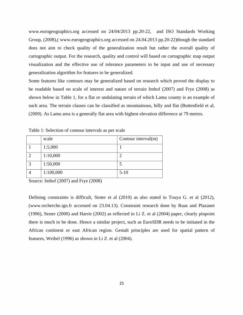
Some features like contours may be generalized based on research which proved the display to
be readable based on scale of interest and nature of terrain Imhof (2007) and Frye (2008) as
shown below in Table 1, for a flat or undulating terrain of which Lamu county is an example of
such area. The terrain classes can be classified as mountainous, hilly and flat (Buttenfield et al,
(2009). As Lamu area is a generally flat area with highest elevation difference at 79 metres.
Table 1: Selection of contour intervals as per scale
scale Contour interval(m)
1 1:5,000 1
2 1:10,000 2
3 1:50,000 5
4 1:100,000 5-10
Source: Imhof (2007) and Frye (2008)
Defining constraints is difficult, Stoter et al (2010) as also stated in Touya G. et al (2012),
(www.recherche.ign.fr accessed on 23.04.13). Constraint research done by Ruas and Plazanet
(1996), Sester (2000) and Harrie (2002) as reflected in Li Z. et al (2004) paper, clearly pinpoint
there is much to be done. Hence a similar project, such as EuroSDR needs to be initiated in the
African continent or east African region. Gestalt principles are used for spatial pattern of
features, Weibel (1996) as shown in Li Z. et al (2004).

26
CHAPTER 3: METHODOLOGY The data used in generalization was collected using instruments stated below, at the initial survey
and map revision periods. The data was then subjected to Cartographic Generalized.
3.1.0 Measuring equipment and Materials used in Collecting Base data for Generalization • Handheld Ashtech GPS receiver
• Geodetic GPS Receiver(3 sets)
• 4 manuscripts of Topographical sheets for Lamu area, sheet 180/1-4 at scale of 1:50,000.
• Field book, pen and pencil
• Rectified and Geo-referenced Aerial Image (by use of LIDAR technology) & other data
of the AOI at photogrammetric scale of 1:5,000 and Ground Sampled Distance (GCD) of
within 25 cm, dated March 2011. Base data created at scale of 1:5,000 for generalization
3.1.1 Source of Geospatial data Survey of Kenya was the main source for Topographic and base datasets used and includes:-
• Base data at the lower level of detail 1:5,000 for the AOI only.
• 4 Sheets of Manuscript of Lamu 180/1-4 at scale of 1:50,000
• Aerial image data compresed format with .ecw extention.
3.1.2 Softwares and Hardware These were used for analysis and processing of the data/ observations and they include the
following:-
• 3 desktop computers with Window 7 OS ,MS office and ArcGIS/ QGis/Global Mapper
Software installed-One is used for local server for data, especially aerial photos, while the
second for data processing and the portable laptop for visualization display in presentations.
• ADOBE CS5 Photoshop- for mosaicing and cleaning of data and other pre-processing
operations.
• ArcGIS 10 Software-for carrying out of the processing and generalization procedures.
• QGis Software- for carrying out of the processing and generalization procedures for light
shape files which require less rendering.
• Global Mapper 10, for surface modelling for DEMS, Grids and Contours.
27
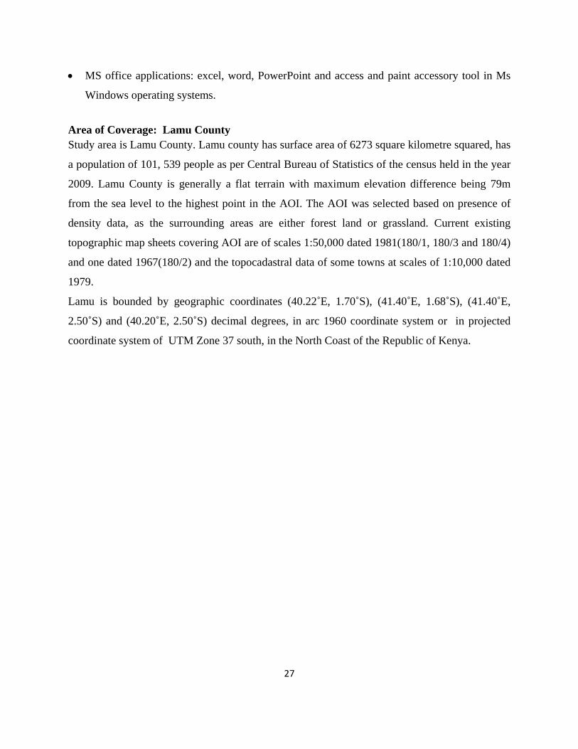
• MS office applications: excel, word, PowerPoint and access and paint accessory tool in Ms
Windows operating systems.
Area of Coverage: Lamu County Study area is Lamu County. Lamu county has surface area of 6273 square kilometre squared, has
a population of 101, 539 people as per Central Bureau of Statistics of the census held in the year
2009. Lamu County is generally a flat terrain with maximum elevation difference being 79m
from the sea level to the highest point in the AOI. The AOI was selected based on presence of
density data, as the surrounding areas are either forest land or grassland. Current existing
topographic map sheets covering AOI are of scales 1:50,000 dated 1981(180/1, 180/3 and 180/4)
and one dated 1967(180/2) and the topocadastral data of some towns at scales of 1:10,000 dated
1979.
Lamu is bounded by geographic coordinates (40.22˚E, 1.70˚S), (41.40˚E, 1.68˚S), (41.40˚E,
2.50˚S) and (40.20˚E, 2.50˚S) decimal degrees, in arc 1960 coordinate system or in projected
coordinate system of UTM Zone 37 south, in the North Coast of the Republic of Kenya.

28
Map of Lamu County
Figure 8: Map of Lamu County showing area of interest bounded in a rectangle.

29
Grid Layers
Figure 8: Map of Lamu County showing area of interest bounded in a rectangle

30
Figure 9: Lamu Grid map layers with point location of some towns
Grid layers are extents to which features cover within a fixed paper size for all scales of
generalization. The grid layers are used in planning the numbering of sheets and visualization of
the representations on the area of interest. The grid layers are further used to delineate various
scales of mapping in the area of interest as shown in figure 9.
EuroSDR (www.eurosdr.net) project is a project on generalization on the state of the art of
automated generalization among universities, NMAs and institutes in Europe. In the EuroSDR
Grid Layers
The grid layers have various
grid cell size extents which
cover defined scales of level of
detail. Topographic features to
be generalized include
administration boundaries,
buildings, railways, roads,
relief, lakes, river, coastal
feature and land cover. Stages
used in generalization process
include modelling, execution
and evaluation. Constraints to
be formalized include those of
minimum sizes, shape, pattern,
distribution, and network.
31
project, there is target dataset, different output results and expert opinion based on importance
and priority on generalization.
Cartographic Constraints
Cartographic constraints are guidelines for the generalization of specific features, which
determine the use of appropriate generalization algorithms (operators).Cartographic constraints
can be set, such as minimum sizes of buildings, minimum distance between buildings, minimum
distance between buildings and roads, keeping building alignment and spatial distribution of
buildings.
Also other than the constraints, map specifications were used to model the constraints in order to
produce cartographically aesthetic product.
3.1.3 Data preparation and matching Landscape model data at scale of 1:5,000 was stored in a folder and then manipulated to depict
other different cartographic models through creation of feature datasets for various feature
classes (layers), which some had their representations created. Furthermore some of the layers
have feature representations as sub categories of the layers. Each layer representation symbology
was defined prior to generalization by digitization for small scales while for some layers; direct
generalization was used especially on simplification of line and polygon feature classes.
3.1.2 Creation of Grid Layers In creation of grids, base information used was scale of 1:50,000 topographic sheets in
geographic coordinate system, which was then subsequently transferred to projected universal
transverse Mercator coordinate system after creation of grid cells for each scale. In
transformation of the sheet scales grids, some calculation for grid size was done based on a
square. After assessing SOK topographical map sheets of scales of 1:50,000, it was noted that
they had grid sizes covering 55.5 (cm) cent metre squared grid, which was be modelled to
accommodate other scales. Also, noted was that, the sheets of 1:50,000 has grid rectangular size
15’ (read as 15 minutes) and has 5 sheets covered in 0.25’ hence each sheet has 0.05’ grid size
containing 25 sheets. Also, the grid cell size for scale of 1:10,000 would be given by 3’/60 which
give 0.05’ grid size with 25 sheets covering in the scale of 1:50,000 and 100 sheets to cover the

32
scale of 1:100,000. Similarly, grid cell sizes for scale of 1:100,000 is 0.5’ (that is 0.25’ multiply
by 2) and 1: 5,000, 1.5’/60 gives 0.025’ grid cell size.
Calculation example showing how grid cell sizes obtained
For scale of 1:10,000 calculation of grid cell size is as shown below:-
Taking that map drawing units is in mm (millimetres) then
To get grid cell size for scale 1:10,000
Take 555= (555x10, 000)/1000=5550 m (metre) grids as shown in the table 2.
Gridding is necessary so as to create available space for each scale representation or calculate the
required generalization and the number of features to represent and general arrangement of map
sheets. One has to set standards to obtain data for schema and items for data collection which are
scale dependent, but this will not be covered since it is beyond the scope.
An example showing how ArcGIS Fishnet tool is used to create the grids is shown in figure 10,
below for the scale of 1:10,000 and inputs of parameters are calculated based on type of scale
and extent. The input parameter indicates the number of sheets to cover in the scale to be used to
add data layers.

33
Figure 10: Grid layer Creation for Scale 1:10,000 using ArcGIS create fishnet
The ArcGIS create fish net tool is used to generate grid layer for all scales of interest. They are scale dependent and can be used to clip the shapes of layers visible, at the data frame properties’ settings, in the final stages of map layout content design. They are also used to create index table for the maps sheets reference inset, of adjoining sheet.
3.1.5 Data identification Data was collected and assembled in one folder. The data collected included aerial imagery from
which a mosaic was made, over which layers were digitized and superimposed. Gridding of the
sheets was done. The procedure for gridding is as shown below. It comprises generating grid cell
sizes for each scale using a standard format of 55.5cm (square). The specification for gridding is
shown in the table below for different scales.
The creation of the fishnet
grid requires one to put
correct parameters; otherwise
a wrong grid would be
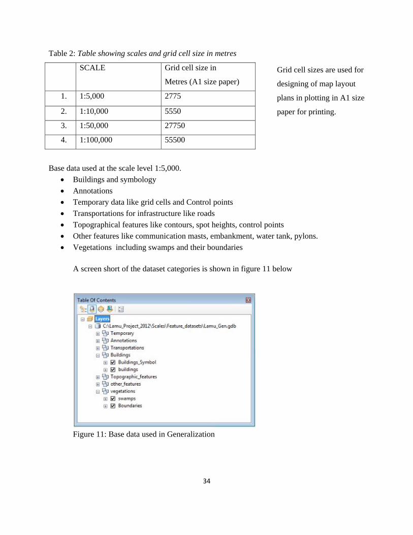
34
Table 2: Table showing scales and grid cell size in metres
SCALE Grid cell size in
Metres (A1 size paper)
1. 1:5,000 2775
2. 1:10,000 5550
3. 1:50,000 27750
4. 1:100,000 55500
Base data used at the scale level 1:5,000. • Buildings and symbology • Annotations • Temporary data like grid cells and Control points • Transportations for infrastructure like roads • Topographical features like contours, spot heights, control points • Other features like communication masts, embankment, water tank, pylons. • Vegetations including swamps and their boundaries
A screen short of the dataset categories is shown in figure 11 below
Figure 11: Base data used in Generalization
Grid cell sizes are used for
designing of map layout
plans in plotting in A1 size
paper for printing.

35
Generalization of the above data sets for various feature classes were represented in feature
representation symbology display and were set to display at scales of 1:5,000, 1:10,000, 1:50,000
and 1:100,000. Using symbol level settings one sets the visibility of the representation layers.
Due to difficulties in generalizing data seamlessly from one digital landscape model (DLM) to
various cartographic representations data was prepared such that each scale had individual DLM.
One can opt to set scale settings, for cartographic zooming as shown in the figure 12 below.
Figure 12: Scale setting to set layer to be visible only when zooming to the scales set.
Similarly one set the data frame properties to view at fixed scales which have settings on whether
the data frame extent will need to be defined or not and such setting such as whether clipping
should occur or not for the shape of extent defined. At the scale of 1: 10,000 the data included
most of the data at base scale; 1:5000, but density reduced like for example the spot heights and
contour coverage.
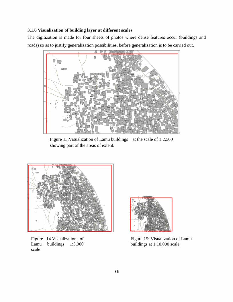
36
3.1.6 Visualization of building layer at different scales The digitization is made for four sheets of photos where dense features occur (buildings and
roads) so as to justify generalization possibilities, before generalization is to be carried out.
Figure 13.Visualization of Lamu buildings at the scale of 1:2,500 showing part of the areas of extent.
Figure 14.Visualization of Lamu buildings 1:5,000 scale
Figure 15: Visualization of Lamu buildings at 1:10,000 scale

37
It is noted from the figures 13-17, showing the same area of extent that visualizations of the area
mapped is fixed, but as scale change is variant there is decrease of paper space for buildings.
The area represented (in the above figures) is a representation (of the same area) of some Old
Lamu Buildings but as scale reduces area for buildings reduces. Furthermore as the scale
decreases the features become blurred and recognition of individual graphics is reduced or
difficult. This can only be enhanced by showing only relevant and necessary details (by
abstraction) which can communicate effectively the use of the representation through a
customized generalization approach for each feature and enhance display by reducing contrast of
the layer.
Effect of the Grid layers on the area of extent covered on a fixed paper size of A1 on various
scales is as shown below. Grid scale plans expected are as shown in the figure below.
A4 SIZE SCALE 1:10,000 A4 SIZE SCALE 1:50,000 A4 SIZE SCALE 1:100,000
Figure 18a: Grid layers on a fixed paper size on scales of 1:10,00, 1:50,000 and 1:100,000.
Figure 16: Visualization of Lamu buildings at 1:50,000 scale
Figure 17: Visualization of Lamu buildings at 1:100,000 scale

38
A4 SIZE SCALE 1: 5,000
From the figure 18a and 18b of grid layers, for each scale transition, there is a decrease in
amount of detail to be discerned clearly as the scale decreases; since as the grid coverage is
reduced so is its details. Grids are drawn at varying scales and extents as the paper space is kept
constant when scale reduces.
The research aims at generalization of base data provided by Survey of Kenya at various scales
starting at 1:5000, then 1:10,000, 1:50,000 and 1:100,000 scales using generalization tools
incorporated in GIS softwares. This will be done by assembling the base data in one location.
Calculation of extents for each of the scales in form of grid scales and then cartographic
generalization operations were used to generalize data cartographically. The data to be
generalized include contours, roads, spot heights, buildings and hydrology features. In some
cases generalization was done through deletion or cartographic pruning, simplification,
amalgamation (aggregation), dissolving among others.
The methodology used in manipulating the data, from data identification to evaluation of results
from generalization algorithms through generalization is as shown below:-
Figure 18b: Grid layers on a fixed paper size on a scale of 1:5,000
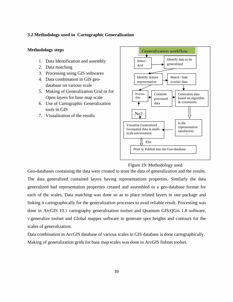
39
3.2 Methodology used in Cartographic Generalization
Methodology steps
Figure 19: Methodology used
Geo-databases containing the data were created to store the data of generalization and the results.
The data generalized contained layers having representations properties. Similarly the data
generalized had representation properties created and assembled in a geo-database format for
each of the scales. Data matching was done so as to place related layers in one package and
linking it cartographically for the generalization processes to avail reliable result. Processing was
done in ArcGIS 10.1 cartography generalization toolset and Quantum GIS/QGis 1.8 software,
v.generalize toolset and Global mapper software to generate spot heights and contours for the
scales of generalization.
Data combination in ArcGIS database of various scales in GIS database is done cartographically.
Making of generalization grids for base map scales was done in ArcGIS fishnet toolset.
1. Data Identification and assembly 2. Data matching 3. Processing using GIS softwares 4. Data combination in GIS geo-
database on various scale 5. Making of Generalization Grid or for
Open layers for base map scale 6. Use of Cartographic Generalization
tools in GIS 7. Visualization of the results
Else
Generalization workflow
Select AOI
Identify data to be generalized
Identify feature representation
Match / link/ overlay data
Combine processed data
Print or Publish into the Geo-database
Process data
Generalize data based on algorithm & constraints
Visualize Generalized Geospatial data in multi-scale environment
Is the representation satisfactory ry y?
No?

40
3.2.1 Generalization Toolsets overview Suggested cartographic generalization tools used are as shown in the figure 20 below. The results
where then visualized and comments were drawn from the same.
Figure 20: Some of the generalization tool in ArcGIS Software.
3.2.2 Overview of the generalization toolset in ArcGIS 10 and Qgis 1.8 softwares An Overview of the generalization toolset found in arcGIS Desktop software in geo-processing tool of cartography toolbox is found in the table 3 below.

41
Table 3: ArcGIS 10.1 Tools in the Generalization toolset
Aggregate Points Creates polygon features around clusters of proximate point features.
Aggregate Polygons
Combines polygons within a specified distance of each other into new polygons.
Collapse Dual Lines To Centerline
Derives centerlines from dual-line (or double-line) features, such as road casings, based on specified width tolerances.
Collapse Road Detail
Collapses small, open configurations of road segments that interrupt the general trend of a road network, such as traffic circles, for example, and replaces them with a simplified depiction.
Delineate Built-Up Areas
Creates polygons to represent built-up areas by delineating densely clustered arrangements of buildings on small-scale maps.
Create Cartographic Partitions
Creates a mesh of polygon features that cover the input feature class where each polygon encloses no more than a specified number of input features, determined by the density and distribution of the input features.
Merge Divided Roads
Generates single-line road features in place of matched pairs of divided road lanes.
Simplify Building Simplifies the boundary or footprint of building polygons while maintaining their essential shape and size.
Simplify Line Simplifies lines by removing extraneous bends while preserving essential shape.
Simplify Polygon Simplifies polygons by removing extraneous bends while preserving essential shape.
Smooth Line Smooths sharp angles in lines to improve aesthetic or cartographic quality.
Smooth Polygon Smooths sharp angles in polygon outlines to improve aesthetic or cartographic quality.
Thin Road Network
Generates a simplified road network that retains connectivity and general character for display at a smaller scale.
Source: ESRI, arcGIS online resource centre, (2012) ArcGIS Help 10.1
42
Overview of generalization toolset in Quantum GIS (Qgis) 1.8
Description of parameters used in Quantum GIS 1.8
threshold=float, Maximal tolerance value, Options: 0-1000000000
look_ahead=integer, Look-ahead parameter, Default: 7
reduction=float, Percentage of the points in the output of 'douglas_reduction' algorithm,
Options: 0-100, Default: 50
slide=float, Slide of computed point toward the original point, Options: 0-1, Default: 0.5
angle_thresh=float, Minimum angle between two consecutive segments in Hermite method,
Options: 0-180, Default: 3
degree_thresh=integer, Degree threshold in network generalization, Default: 0
closeness_thresh=float, Closeness threshold in network generalization, Options: 0-1, Default: 0
betweeness_thresh=float, Betweeness threshold in network generalization, Default: 0
alpha=float, Snakes alpha parameter, Default: 1.0
beta=float, Snakes beta parameter, Default: 1.0
iterations=integer, Number of iterations, Default: 1
layer=integer, Layer number, a single vector map can be connected to multiple database tables.
This number determines which table to use. Default: 1
cats=range, Category values, such as: 1,3,7-9,13
where=sql_query, WHERE conditions of SQL statement without 'where' keyword, Example:
income < 1000 and inhab >= 10000.
Source: Quantum GIS 1.8 user manual. (http://www.qgis.org/en/documentation/manuals.html)
v.generalize tool is found in the Sextante toolbox of Qgis software and it contains simplification
and smoothing algorithms for generalization.
An overview of v.generalize, the Vector generalization tools in Qgis 1.8 for simplification is
provided below.
• Douglas-Peucker – it is a type of line simplification and is the most widely used
algorithm.

43
• Douglas-Peucker Reduction Algorithm is essentially the same Douglas-Peucker
algorithm differing in the case where it takes an additional reduction parameter which
denotes the percentage of the number of points on the new line with respect to the
number of points on the original line.
• Lang - Another standard algorithm for generalization.
• Vertex Reduction - It is a simple algorithm described such that for a given a line, this
algorithm removes the points of this line which are closer to each other than threshold.
More precisely, if p1 and p2 are two consecutive points, and the distance between p2 and
p1 is less than threshold, it removes p2 and repeats the same process on the remaining
points.
• Reuman-Witkam - This algorithm preserves the global characteristics of the lines.
An overview of v.generalize, the Vector generalization tools in Qgis 1.8 for Smoothing
The following smoothing algorithms are implemented in v.generalize:
• Boyle's Forward-Looking Algorithm - The position of each point depends on the position
of the previous points and the point look_ahead ahead. look_ahead consecutive points.
• McMaster's Sliding Averaging Algorithm - The new position of each point is the average
of the look_ahead points around. Parameter slide is used for linear interpolation between
old and new position (see below).
• McMaster's Distance-Weighting Algorithm - Takes the weighted average
of look_ahead consecutive points where the weight is the reciprocal of the distance from
the point to the currently smoothed point. The parameter slide is used for linear
interpolation between the original position of the point and newly computed position
where value 0 means the original position.
• Chaiken's Algorithm - "Inscribes" a line touching the original line such that the points on
this new line are at least threshold apart.. This algorithm approximates the given line very
well.
• Hermite Interpolation - This algorithm takes the points of the given line as the control
points of hermite cubic spline and approximates this spline by the points
approximately threshold apart. This method has excellent results for small values

44
of threshold, but in this case it produces a huge number of new points and some
simplification is usually needed. Angle_thresh, an input parameter, is used for reducing
the number of the points. It denotes the minimal angle (in degrees) between two
consecutive segments of a line.
• Snakes is the method of minimisation of the "energy" of a line. This method preserves the
general characteristics of the lines but smooths the "sharp corners" of a line. Input
parameters input, alpha, beta. This algorithm works very well for small values
of alpha and beta (between 0 and 5). These parameters affect the "sharpness" and the
curvature of the computed line.
Source: Quantum GIS 1.8 user manual. (http://www.qgis.org/en/documentation/manuals.html)
3.2.3 Cartographic Generalization of Base data at scale 1:5,000 What was subjected to generalization include polygon, line and point features. Vector layers to
be generalized were first copied and stored in on folder for each scale level, that is, 1:10,000,
1:50,000 and 1:100,000 scales. Then a file geo-database was created, where all the datasets for
topographic ,buildings, transportations, water, vegetations, administration boundaries, temporary
features like grid, index diagrams and other features like communication masts, pylons and
embankment were imported into together with their symbolization. Though manual computer
generalization was done it affected features like annotation elements, text and spot heights by
reducing their density. Furthermore, some features were retained like location of Manda airport
while others were deleted all together like culvert, ditches, borehole and water level. Application
of generalization algorithm was done on each whole layer individually, each requiring different
generalization toolset with specific tolerance or constraints for each scale under consideration.
Majorly, generalization was effected on the following types of feature classes.
How generalization was effected is shown below along feature classes considered. In setting up
display for the scales specified, one sets the viewing scale ranges in the layer settings and in the
data frame.

45
3.2.4 Buildings Generalization Building generalization composed of building simplification where three types of polygon
simplification were used: Eliminate polygon part by area, percent and area or percentage
tolerances for the three scales 1:10,000, 1:50,000 and 1:100,000. The constraint parameters for
the three scale used are as shown in the table below.
Table 4: Building simplification constraints used
Scale Area of buildings deleted(m²) Percentage (%) Area or percentage 1. 1:10,000 80 50 80m² 2. 1:50,000 400 - - 3. 1:100,000 800 - -
Other tools uses include Building Simply, simplify polygon, delineate built-up areas, and
building aggregation at 20 metres aggregation among others.
3.2.5 Shoreline simplification In shoreline generalization two line simplication criteria were used; simplification and
smoothing. Simplification was by bendSimplify and point remove and smoothing was done
using smooth line using Bezier interpolation.
Table5: Shoreline line simplification by Bendsimplify and point remove
Scale Bendsimplify:
Reference baseline
Point remove:
Maximum allowable offset
1. 1:10,000 80 80m²
2. 1:50,000 100 -
3. 1:100,000 100 -
Also considered is smooth line generalization, where the smooth line tool was used to smooth
sharp angles and enable to produce cartographically aesthetic quality map. The smooth line tool
does not require tolerance specification and hence can be used in all scales. The only
preconditions to be used include smoothing the shoreline using Bezier interpolation with
flagging of topology errors if present after generalizing the shoreline using simplification tool on
the layer.
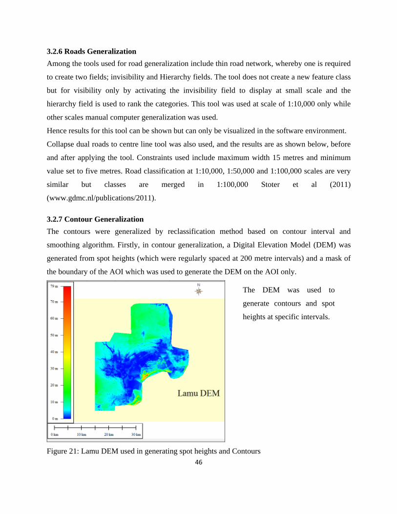
46
3.2.6 Roads Generalization Among the tools used for road generalization include thin road network, whereby one is required
to create two fields; invisibility and Hierarchy fields. The tool does not create a new feature class
but for visibility only by activating the invisibility field to display at small scale and the
hierarchy field is used to rank the categories. This tool was used at scale of 1:10,000 only while
other scales manual computer generalization was used.
Hence results for this tool can be shown but can only be visualized in the software environment.
Collapse dual roads to centre line tool was also used, and the results are as shown below, before
and after applying the tool. Constraints used include maximum width 15 metres and minimum
value set to five metres. Road classification at 1:10,000, 1:50,000 and 1:100,000 scales are very
similar but classes are merged in 1:100,000 Stoter et al (2011)
(www.gdmc.nl/publications/2011).
3.2.7 Contour Generalization The contours were generalized by reclassification method based on contour interval and
smoothing algorithm. Firstly, in contour generalization, a Digital Elevation Model (DEM) was
generated from spot heights (which were regularly spaced at 200 metre intervals) and a mask of
the boundary of the AOI which was used to generate the DEM on the AOI only.
Figure 21: Lamu DEM used in generating spot heights and Contours
The DEM was used to
generate contours and spot
heights at specific intervals.

47
Using various contour intervals for the three scales, a contour surface was generated for scales of
1:10,000, 1:50,000 and 1:100,000 at contour intervals of 4 metres, 20 metres and 40 metres
respectively based on Directorate of Ordinance Survey general specifications for terrain.
Labelling and symbolizing for the contours was done along the contour with a hallo mask style
of size 2.000. It was noted that contours at the smaller scales were sparse , hence contours were
again generated using specifications proposed by Imhof(2007) and Frye(2008) for flat and
undulating terrain at contour intervals of 2 metres, 5 metres and 10 metres for scales of 1:10,000,
1:50,000 and 1:100,000 respectively to increase coverage of contours.
3.2.8 Spot height Generalization Spot heights were generated after generating a DEM. The process involved using AOI and spots
heights extent which on loading them at the software, they were selected, and an elevation grid
for 3D vector data was generated at varied intervals of 400 metres, 1000 metres and 2000 metres
respectively for the scales of 1:10,000, 1:50,000 and 1:100,000. Then, point features at elevation
grid centres were created from which interpolated point features were exported as point features
spaced at the specified intervals for each category.
When to generalize is governed by displaying the details at the scale of choice with clear legible
map. Other feature line symbols for building were manually deleted when they occupied some
areas of the map causing black white ratio to fall over acceptable tolerance.
Also vector based generalization was carried out using QuantumGIS 1.8. using Douglas Peucker
algorithm is shown in the figure below with a Qgis scripting page
.

48
Figure 22: v.generalize algorithm generalization script in Qgis for roads
Visual examination of Figure 22, the scripting page is not clear as the tools are in trial stages and the execution of the tool operation shows the process status script in a faint font.

49
CHAPTER 4: RESULTS AND DISCUSSIONS
4.0 Vector Feature Generalization Results In the discussion above, various cartographic generalization tools were used dependent on
license capabilities and upgrade or edition type of the software. The general work flow of the
generalization process was carried depending on user requirements; the process can also be
applied in different places using different abstraction scales which represent the same area.
In addition creation and keeping of a single Digital Landscape model for each of the scales in a
single geo-database was complex and hence needs a logical framework on the storage locations
for each of the datasets and the manipulation processes to be uniquely identified by the software
in operation. For this case separate file geo-database was used for deriving each scale datasets.
Figure 23: Location Diagram and Index to adjoining sheets at scale of 1:10,000, Sheet no. 57.
4.1 Building Generalization Results Building generalization was applied by selecting building layers to be generalized and then
operations algorithms such as aggregation, and simplification were chosen. The criterion used
was based on building area, taking the whole layer or global constraint. Global selection of layer
was used in effecting building generalization operation done at Scale: 1:10,000, 1:50,000 and
Sheets with one sheet
numbered 180/10/57 for
demonstration is selected
and is superimposed with
Lamu County as area of
interest

50
1:100,000. Some of the building generalization for the scale of 1:10,000, using aggregation
operation at 5m is as shown below.
Figure 24: Building aggregation at 5metres.
Buildings do not retain normal true area extent; they have some aggregation on geometry as
buildings are combined, irrespective of type.
Also building simplification was carried at 10 metres and the result looks similar as previous
example.
Figure 25: Building Simplify at 10 metres
Building generalization by simplifies building operation was not done at the scale 1:100,000
because of inability to preserve areal size of features. Combining or converting to points looks as
shown below and makes it necessary to select which type of buildings to show at the scale.

51
Figure 26: Building conversion to point using Polygon to point conversion tool.
Further, by eliminating some of the points which are eliminated by putting a constraint that a
building less than 400 metre squared to be removed and the others are retained. The following is
what is realized after selecting only a few of them
Figure27: Building point generalization
As seen from the above it can be noticed that individual building recognition becomes difficult
as one reduces scale, unless the map is made thematic, hence individual buildings cannot be
shown at scale 1:100,000. Aggregation and erase points are used instead for displaying
aggregated, converted to points and those in built up areas.
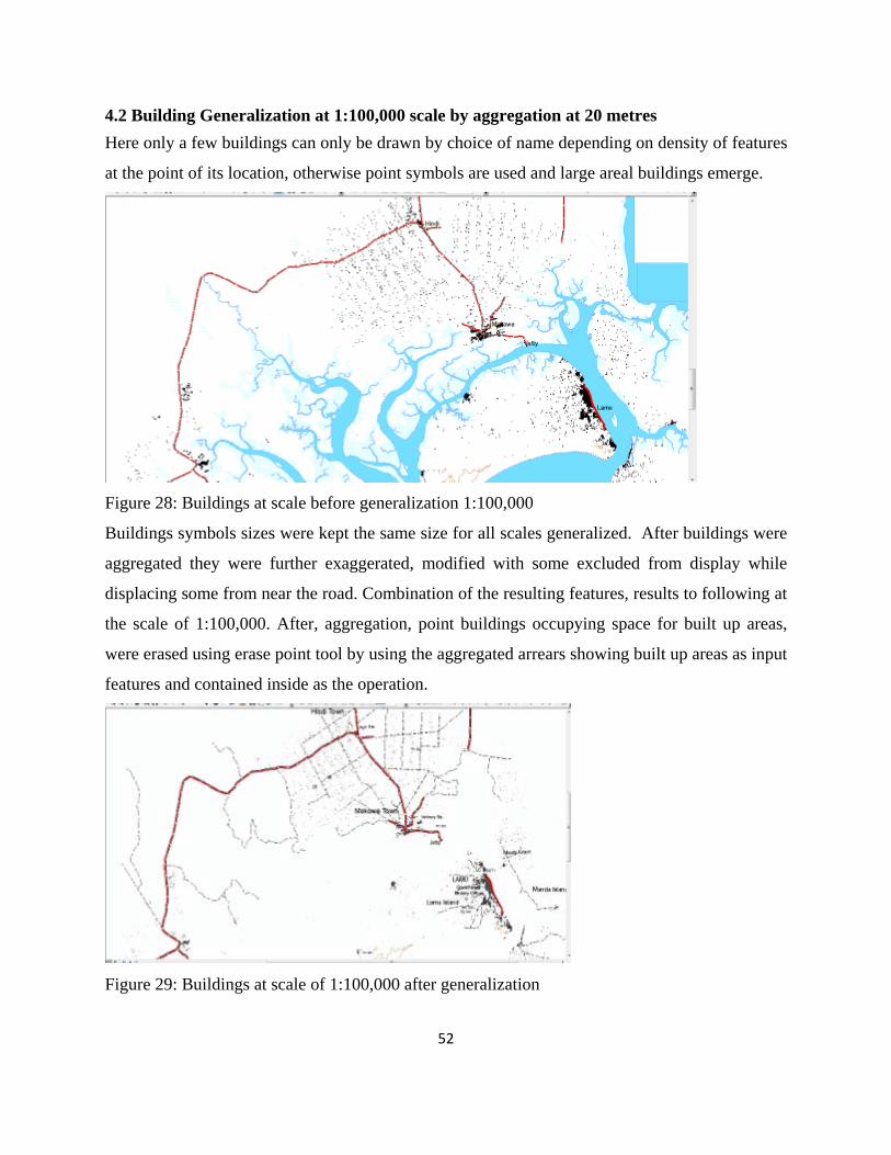
52
4.2 Building Generalization at 1:100,000 scale by aggregation at 20 metres Here only a few buildings can only be drawn by choice of name depending on density of features
at the point of its location, otherwise point symbols are used and large areal buildings emerge.
Figure 28: Buildings at scale before generalization 1:100,000
Buildings symbols sizes were kept the same size for all scales generalized. After buildings were
aggregated they were further exaggerated, modified with some excluded from display while
displacing some from near the road. Combination of the resulting features, results to following at
the scale of 1:100,000. After, aggregation, point buildings occupying space for built up areas,
were erased using erase point tool by using the aggregated arrears showing built up areas as input
features and contained inside as the operation.
Figure 29: Buildings at scale of 1:100,000 after generalization

53
The one delineating built up areas at 20 metres is shown below in a few clusters of irregular
polygons created.
Figure 30: Delineating Built-up areas using 20 metres as tolerance
The figure 30, above shows delineating Built-up areas using 20 metres as tolerance for display at
larger scale of 1:50,000 scale after zooming in the display.
On comparing the last result with one of manual editing after using aggregate polygon tool gives
the following results; which are almost similar with the results shown above of delineating built-
up areas at 50 metres
.

54
Figure 31: Delineating built-up areas using 50 metres torelance for display at smaller scale of
1:100,000.
The two results are of delineation are as shown below
Figure 32: Superimposing the layers after aggregation
The results are compared with use of manual editing and built up areas tools for display at scale
level 1:100,000. Which can also be shown at a smaller scale of 1:50,000, but zoomed as shown
below to reflect, the effect of the tool in delineating built up areas.

55
Figure 33: Building generalization by use of delineate built-up area tool
4.3 Road Generalization details Road generalization was be done through deletion or selective pruning or checking or un-
checking in the layout or data visualization in the suggested generalization scales.
Scale: 1:10,000
Most of the foot paths are eliminated from the display using collapse Dual lines to centreline
generalization tool. It is noticeable that most foot paths are retained where there are junction
points unlike where there are no junctions.
Figure 34: Roads Generalization process success dialog

56
From above dialog, generalization result can be assessed in real time, since at the end of the
process, the tool responds whether the generalization was successful or not. In cases where it is
not successful, tool also responds together with detailed report citing reasons for any eventuality
of error.
Collapse Dual lines to centerline tool, the tool generates a feature layer with four new fields
which need ranking information on line type; align right or left and polyline ids at their default.
The results after applying the collapse Dual line to centre line and zooming the map display to
1:250,000 yields the following illustrations.
Figure 35: v.generalize algorithm, using network method of generalization operation in Qgis for representing roads for scale of 1:10,000.
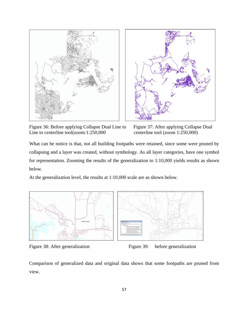
57
Figure 36: Before applying Collapse Dual Line to Figure 37: After applying Collapse Dual Line to centerline tool(zoom:1:250,000 centerline tool (zoom 1:250,000) What can be notice is that, not all building footpaths were retained, since some were pruned by
collapsing and a layer was created, without symbology. As all layer categories, have one symbol
for representation. Zooming the results of the generalization to 1:10,000 yields results as shown
below.
At the generalization level, the results at 1:10,000 scale are as shown below.
Figure 38: After generalization Figure 39: before generalization
Comparison of generalized data and original data shows that some footpaths are pruned from
view.

58
Figure 40: Collapse of dual roads to centreline overlay with initial data at scale 1:5,000.
Only Major road type like tarmac, earth and motorable tracks are retained as foot paths are
eliminated. This was done manually to preserve general geometry.
Figure 41: Road Generalization at Scale 1:50,000 and 1:100,000.
At the scale of 1:10,000, only the Tarmac, Earth and a few motorable tracks type of roads were
retained.

59
Figure 42: Generalized map with all the layers generalized at the scale of 1:100,000.
4.4 Contour Generalization Results Contour generalization was done through use of reclassification whereby there was variation of
contour interval and the number of spot heights coverage selection by automatic selective
deletion or distribution in the area of interest. The contours were generalized using
reclassification method by using spot heights of the AOI to make a Digital Elevation Model
(DEM), whereby contours were generated using Global Mapper 12 mapping software. The
results are as shown below. General specifications were used but specific specification suited for
flat areas, as proposed by Imhof (2007) and Frye (2008) were also used to produce the final
generalized contours. The visualization of the results is as shown below, with zoom of 1:250,000
scale so as to show the general distribution of all contours in the AOI.
Contour generalization results zoomed to scale 1:250,000 using general specifications.

60
1:5,000 scale 1:10,000 scale
1:50,000 scale 1:100,000 scale
Figure 43: Contour Generation for smaller scales using general specifications
Results of contour generalization using Survey of Kenya general specifications on contours show
that, for a generally flat terrain, like Lamu area, the contours will be visible at the scale of
1:10,000. Similarly contour generation at scale of 1:50,000, results to sparse contours and at
1:100,000 almost disappear because of a large contour interval, 40 metres. These made the use of
alternative method proposed by Imhof(2007) and Frye(2008) which enables one to get contours
at intervals suited for flat terrain.

61
Contour generalization results
1:5,000 scale 1:10,000 scale
1:50,000 scale 1:100,000 scale
Figure 44: Contour generation using specification suited for flat areas in contouring, as proposed
by Imhof (2007) and Frye (2008).
From the above, it can be noticed that as one traverse from lager scale to smaller scale contours
diminish. Other features will be deleted and they include culverts, ditches, piers, any non
important details in the smaller scales of 1:50,000 and 1:100,000.

62
Also, other features will be grouped and other re-created or introduced such as spot heights.
Other features retain their states and they included swamps, vegetation boundaries and ocean
boundaries and what can be changed can be sizes of symbols used to depict the features.
4.5 Spot height Generalization results
1:5,000 scale 1:10,000 scale
1:50,000 scale 1:10,000 scale
Figure 46: Spot height generalizations from base scales of 1:5,000 to scale of 1:10,000, 1:50,000 and 100,000 using general observation of distribution.

63
The spot height generation like contour generalization used intervals in generalization. From the
generalization, whereby, results for whole area of interest zoomed at scale of 1:250,000, shows
satisfactory results as number of points decreased from 20,827 points with scale such that as
shown number of feature count for each scale is 5234, 833 and 213 points respectively for scales
of 1:10,000, 1:50,000 and 1:100,000.
4.6 Shoreline Generalization details Shore line simplification based on 50 metres offset and with bend simplify for view at scale of
1:50,000 and check topographical errors and resolve topographical error options checked or
selected. The shoreline so simplified was then smoothened based on Bezier interpolation
technique.

64
Shoreline generalization results
Figure 46: Shoreline simplifications for scales of 10k, 50k and 100k
Result of bend simplify simplification algorithm followed by smoothing using Bezier
interpolation was used.
Figure 47 below shows the maps generalized.
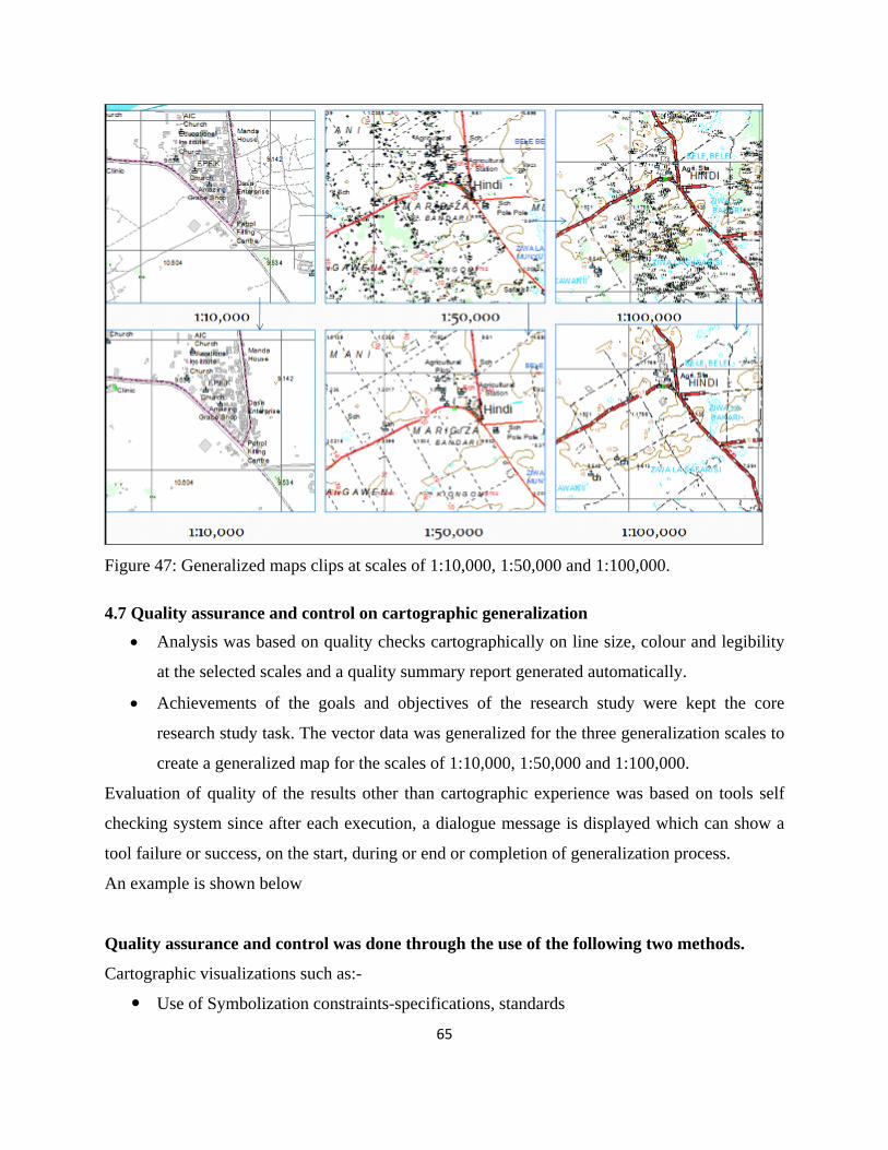
65
Figure 47: Generalized maps clips at scales of 1:10,000, 1:50,000 and 1:100,000.
4.7 Quality assurance and control on cartographic generalization • Analysis was based on quality checks cartographically on line size, colour and legibility
at the selected scales and a quality summary report generated automatically.
• Achievements of the goals and objectives of the research study were kept the core
research study task. The vector data was generalized for the three generalization scales to
create a generalized map for the scales of 1:10,000, 1:50,000 and 1:100,000.
Evaluation of quality of the results other than cartographic experience was based on tools self
checking system since after each execution, a dialogue message is displayed which can show a
tool failure or success, on the start, during or end or completion of generalization process.
An example is shown below
Quality assurance and control was done through the use of the following two methods.
Cartographic visualizations such as:-
Use of Symbolization constraints-specifications, standards

66
Visual assessment of the results onscreen and prints
Reference to minimum sizes
Within the software:-
Summary statistics and Map contents summary
Distribution and density on mapping space
Control of generalization process through appropriate tolerances/parameters selection for
operators.
4.8 Challenges encountered in Cartographic Generalization Challenges encountered include design of new symbols for feature description at smaller scale,
minimum size and constraint considerations harmonization and effecting of colour associations
and perceptions in map layout design and decision on what to include or exclude.
Designing new Symbols for each of the scales was a challenge as designing each symbol for
each scale for some features which have their symbols changed was tasking in defining
individual symbol sizes and layout. Symbol selection and size is defined in symbology since
definition of feature attributes, specified sizes and colour attribute choice for each scale,
representation and application is a research topic beyond the scope of the research. Hence
symbols of the base data were adopted, with their sizes minimized and zoomed. Some symbols
sizes were also modified to reflect the content of the map while other symbols like for buildings
were kept constant.
67
CHAPTER 5: CONCLUSION AND RECOMMENDATIONS
5.1 Conclusion Generalization using generalization operators were used for the topographic features suited for
generalization algorithm. After carrying generalization using GIS toolset of simplification,
aggregation, and modification among other operators was successful in generating generalized
map layers contained in a geo-database at the generalization levels of scales.
As per the research, generalization algorithms available in GIS systems are appropriate to
specific types of data as shown below.
• Simplification is suited for line, point, polygon generalization at scale level 1:10,000
• Aggregation for point data 1:10,000, aggregation of buildings or polygon for scale level
scales of1:10,000, 1:50,000 and 1:100,000) or ,
• delineate built up areas 1:50.000 and 1:100,000),
• simplify buildings for scale 1:10,000,
• thin road network for scales of 1:50,000 and 1:100,000,
• collapse road detail and merge divided roads for scales of 1:10,000, 1:50,000 and
1:100,000, modification and smoothing for contours and spot heights for 1:10,000,
1:50,000 and 1:100,000 , smooth line and polygon for scales 1:10,000, 1:50,000 and
1:100,000 and
• collapse dual line road to centerline 1:50,000 and 1:100,000 for roads among others, using
appropriate parameters or constraints and symbolizing using appropriate specifications.
Each of the tools used above are specifically suited for a certain layer type and scale
5.2 Recommendations There is need to define, the minimum sizes for all features contained in topographical maps for
all scales together with the constraint parameter used in generalizing the data based on
specifications and then formalizing the procedures in a well described or documented
cartographic workflow. Need for NMA, SoK, to implement the use of GIS generalization tools
and organizing for training to be provided to achieve the desired products of generalization based
on specifications and standards.

68
REFERENCES
1. Alfred Rytz,(1987), Cartographic generalization of Topographic maps. Swiss Society of Cartography.
2. Bard S. (2004). Quality assessment of cartographic generalisation. Transactions in GIS, 8:63–81, 2004. S. Bard and A. Ruas. Why and how evaluating generalised data? In Developments in Spatial Data Handling (SDH’ 04), pages 327–342. Springer, Leicester.
3. Bard S. and Ruas A. (2004) Why and how evaluating generalized data? In Developing in Spatial Data handling (SDH-04), pp.327-342. Springer, Leicester.
4. Bertolotto, M. (2007). Progressive techniques for efficient vector map data transmission: An
5. Bloch, M., and M. Harrower. (2006). MapShaper.org: A map generalization web service. In: Proceedings of AutoCarto 2006. Vancouver, WA.
6. Brewer C. et al (2010), Designing USGS Topographic Mapping for Multiscale online use, ESRI user conference 2010.
7. Buttenfield B. P. (1991). A rule for describing line feature geometry. In.Buttenfield B. P and McMaster R. B., editors, Map Generalization: Making Rules for Knowledge Representation, pages 150–171. London: Longman.
8. Buttenfield B. P., Brewer C. A. and Stanislawski L. V (2010). Multiscale representations of water: Tailoring generalization sequences to specific physiographic regimes. In:Proceedings of GIScience 2010. Zurich, Switzerland.
9. Buttenfield, B.P(1987) Automating the Identification of Cartographic lines. The American Cartographer, 14(1),7-20.
10. Cromley, R., and Campbell G. 1992. Integrating quantitative and qualitative aspects of digital line simplification. The Cartographic Journal. 29(1): 25–30.
11. Devau, T.J (1985), Reducing the number of points in a plane curve representation. Proceedings of Auto-Cartoo VII, American Congress on Surveying and Mapping, pp. 152-160.
12. Douglas, D. H., and. Peucker T. K. (1973). Algorithms for the reduction of the number of points required to represent a digitized line or its caricature. The Canadian Cartographer. 10(2): 112–122.
13. Dulgheru. F. V, (2011) Algorithms for Map Generalization with ArcGIS Software, International Conference Scientific paper Afases, 26-28 May 2011. Geoint Center, Military Technical Academy, Bucharest, Romania.

69
14. ESRI ArcGIS online Resource centre, (2012) ArcGIS Help 10.1, Available online at: http://resources.arcgis.com, accessed on 12th April 2013.
15. EuroSDR presentation, (2003). available online at www.ifp.uni-stuttgart.de/phowo/presentations/320Heipke.pdf Accessed on 02.12.12
16. EuroSDR, Rollong (2011). Research Plan, 2011-2014, Faculty of the Built Environment, The Dublin Institute of Technology, Bolton Street. Dublin 1 Ireland. Available online at www.eurosdr.net/rrp/eurosdr_research_plan_2011-2014.pdf viewed on 02.12.12
17. Fangli Ying et al (2011). How little is enough? Evaluation of user satisfaction with maps generated by a progressive transmission scheme for geospatial data available online at www.agile.gis.geo.tu-dresden.de accessed in 23.12.12)
18. Foerster T.; Stoter, J. & Kobben B. (2007): Towards a formal classification of Generalization operators. ICC (International Cartographic conference) paper.
19. Foerster, T., Lehto, L., Sarjakoski, T., Sarjakoski, L. T. and Stoter, J. E. (2010). Map generalization and schema transformation of geospatial data combined in a web service context, Computers, Environment and Urban Systems 34(1): 79–88.
20. Frye Charlie. (2008). Producing Cartographic Contours from Elevation Models in ArcGIS. ESRI White Papers
21. Galanda M and Weibel R, (2002) An agent-based framework for polygonal subdivision generalisation In Proceedings of the ISPRS Symposium on Geospatial Theory, Processing and Applications, Ottawa, Ontario, Canada. Geoinformatica, 6(3), pp. 233-261.
22. Goodchild, M.F. 1980, "Fractals and the Accuracy of Geographical Measures", Mathematical Geology, Vol. 12, 85-98.
23. Gruenreich, D. (1992): ATKIS - a topographic information system as a basis for GIS and
digital cartography in Germany. From digital map series to geo-information systems, Geologisches Jahrbuch Reihe A, 207 – 216.
24. Hakanson, Lars, (1978), "The Length of Closed Geomorphic Lines," Mathematical Geology,
Vol. 10, 141-167.
25. Harrie (2001). An Optimisation Approach to Cartographic Generalization. PhD thesis, Lund Institute of Technology.
26. Harrie and Sarjakoski T. (2002). Simultaneous graphic generalization of vector data sets. GeoInformatica, 6(3):233–261.
27. Harrie, L, Sarjakoski, T, and Lehto, L.(2002). A Variable-Scale Map for Small-Display Cartography. In: Proceedings of the Joint International Symbosium on Geeospatial Theory, Processing and Applications. Ottawa.

70
28. Heller, M. (1990). Triangulation algorithms for adaptive terrain modeling. In: 4th International Symposium on Spatial Data Handling (SDH ’90). Zurich, Switzerland: International Geographical Union.
29. Imhof Eduard. (2007). Cartographic Relief Presentation. ESRI Press, Redlands, CA
30. ISO (2003), Geographic information - Rules for application schema ISO.
31. ISO Standards Working Group, (2008),“Guidelines for Implementing the ISO 19100 Geographic Information Quality standards in National and Mapping agencies “in Antti Jakobsson, Jorgen Giversen(ed) available online at www.eurogeographics.org accessed on 24.04.2013 pp.20-22
32. Jenks, G.F. (1979), "Thoughts on Line Generalization," ^Proceedings, AUTO CARTO IV, 209-221.
33. Jones C.B. and I.M. Abraham, (1986). "Design Considerations for a Scale- Independent
Cartographic Database," Proceedings, Second International Symposium on Spatial Data Handling, 384-398.
34. Jones, C (1998). Geographic Information Systems and Computer Cartography. Addison
Wesley, Longman. Singapore. pp 271-289.
35. Jones, C.B. and ABRAHAM, I.M., 1987, Line generalisation in a cartographic database. Cartographica, 24(3), pp. 32–45.
36. Kenya Law Reporting, KLR (2010).The Survey Act, cap.299. Available online at www.kenyalaw.org. accessed on 13.12.12
37. Kilpeläinen, T. (1997). Multiple representation and generalization of geodatabases for topographic maps. PhD Dissertation. Helsinki, Finland: Finnish Geodetic Institute.
38. Kraak M.J. & Ormeling, F.J (1996). Cartography: Visualization of Spatial Data. Longman Singapore Publishers.
39. Lang , T(1969) Rules for Robot Draughtsmen, Geographical Magazine,62(1)50-51.
40. Li Z. , Yan H. , Ai T. & Chen J. (2004): Automated building generalization based on urban morphology and Gestalt theory , International Journal of Geographical Information Science, 18:5, 513-534.
41. Lyndon B. ,(1993) Johnson Space Centre, JSC-25012, CLIPS Basic Programming Guide Version 6.0, Vol. 1
42. Mackaness W. A. and Ruas A.,( 2007). Evaluation in the map generalisation process. In W. A. Mackaness, A. Ruas, and L. T. Sarjakoski, editors, Generalisation of Geographic
71
Information: Cartographic Modelling and Applications, Series of International Cartographic Association, pages 89–111. Elsevier Science, Amsterdam,.
43. Mandebrot B.B(1982) The Fractal Geometry of Nature, W H Freeman and Co. San Francisco.
44. Mandelbrot, B.B. (1982), "The Fractal Geometry of Nature, Freeman, San Francisco
45. Marino,(1979) Identification of Characteristic Points along naturally occurring lines : an empirical study. The Canadian Cartographer, 16(1)70-80
46. Mark Denil (2011). “The Search for a Radical Cartography” in Patrick Kennelly(Ed), Cartography Persipectives. 68. North America Cartographic Information Society, pp. 30 Available online at www.cartographicperspectives.org/index.php/journal/article/...full/84 pp. 30 accessed on 23.02.13
47. McMaster R. B. and K. S. Shea (1992).Generalization in Digital Cartography. Resource Publications in Geography. Association of American Geographers.
48. McMaster, R. (1989). The integration of simplification and smoothing routines in line generalization. Cartographica. 26(1): 101–121.
49. McMaster, R., and M. Monmonier. (1989). A conceptual framework for quantitative and qualitative raster-mode generalization. In: GIS/LIS ’89. Orlando, FL.
50. McMaster, R.B. (1983). "Mathematical Measures for the Evaluation of Simplified Lines on Maps," Unpublished Ph.D. Dissertation thesis, University of Kansas, 333 pages.
51. Monmonier, M. (1991). Ethics and map design. Six strategies for confronting the traditional one-map solution. Cartographic Perspectives. 10: 3–8.
52. Muller J. C, (1986) optimum point density and compaction rates for the representation of geographic line, proceeding of autocarto(1987).
53. Muller J.-C. (1987), "Fractals and Automated Line Generalization", The Cartographic Journal, Vol. 24, in press.
54. Muller, J. C. (1987). Optimum point density and compaction rates for the representation of geographic lines. In Proceedings of AutoCarto (Vol. 8, pp. 221-230).
55. Muller, J., and Wang, Z., (1992), “Area-patch generalization: a competitive approach:, The Cartographic Journal 29, 137-144 overview, in A. Belussi, B. Catania, E. Clementini and E. Ferrari (eds), Spatial Data.
56. Muller, J.C. (1986), "Fractal Dimension and Inconsistencies in Cartographic Line
Representations," The Cartographic Journal, Vol. 23, in press.

72
57. Qian et al (2008). How the Quality of Cartographic Generalization is Assured-The Approach with an Automatic Cartographic Generalization Chain. available online at www.isprs.org/proceedings/XXXVII/congress/2_pdf/3_WG.../10.pdf
58. Quantum GIS 1.8 user manual (2012). Available online at http://www.qgis.org/en/documentation/manuals.html accessed on 15.12. 2012.
59. Regnauld, N. and R. McMaster. (2007). A synoptic view of generalisation operators. In: W. A. Mackaness, A. Ruas, and L. T. Sarjakoski (Eds.) Generalisation of geographic information: Cartographic modelling and applications. Amsterdam, The Netherlands: Elsevier.
60. Reumann, K. and Witkam, A.(1974) Optimizing Curve Segmentation in Computer Graphics. In: International Computing Symposium, PP.467-472.Amsterdam.
61. Richardson D.E (1988) Rule based generalization for base map production, Unpublished Masters’ Thesis, ITC, Enschede.
62. Richardson, L.F. (1961). “The Problem of Contiguity: An Appendix of Statistics of of
Deadly Quarrels," General Systems Yearbook, Vol. 6, 139-187
63. Roth, R., Brewer, C., Stryker, M.(2012) A typology of operators for maintaining legible map designs at multiple scales. Cartographic Perspectives, North America, Jan. 2012. Available online at: http://www.cartographicperspectives.org/index.php/journal/article/view/cp68-roth-et-al accessed: 14.03. 2013.
64. Ruas, (2001). Automatic generalization research: Learning process from interactive generalisation. Technical Report 39, OEEPE.
65. Ruas, A., and Plazanet, C., (1996), Strategies for automated generalization. Proceedings of Spatial Data Handling, 6.1–6.18.
66. Sarjakoski, L. T. (2007). Conceptual models of generalization and multiple representation. In: Mackaness W. A., Ruas A., and Sarjakoski L. T. (Eds.) Generalisation of geographic information: Cartographic modelling and applications. Amsterdam, The Netherlands: Elsevier.
67. Sester(2005). Optimization approaches for generalization and data abstraction. International Journal of Geographical Inforamtion Science, 19(8): 871–897.
68. Skopelity A. and Tsoulos L.,(2000). Developing a model for quality assessment of linear features. In Proceedings of the 4th International Symposium on Spatial Accuracy Assessment in National Resources and Environmental Sciences, pages 655–658.

73
69. Skopelity and L. Tsoulos (2000). Developing a model for quality assessment of linear features. In Proceedings of the 4th International Symposium on Spatial Accuracy Assessment in National Resources and Environmental Sciences, pages 655–658.
70. Skopelity and T. Lysandros (2001) A methodology for the assessment of generalization quality. In The FourthWorkshop on Progress in Automated Map Generalization, Beijing.
71. Stoter et al (2011): A semantic-rich multi-scale information model for topography, International Journal of Geographical Information Science, 25:5, 739-763. Online at http://www.gdmc.nl/publications/2011/Multi-scale_information_model_topography.pdf accessed on 2.12.12.
72. Stoter, J. E. (2005). Generalisation within NMA’s in the 21st century. In: Proceedings of the International Cartographic Conference. A Coruña, Spain.
73. Swiss Society of Cartography (1977), "Cartographic Generalization," Cartographic Publication Series, No. 2. English translation by Allan Brown and Arie Kers, ITC Cartography Department, Enschede,Netherlands).
74. Swiss Society of Cartography, Cartographic Generalization of Topographic maps. Cartographic publication Series number 2.
75. Theodor Foerster & Jantien Stoter, (2008) Generalisation operators for practice – a survey at national mapping agencies, available online at: http://generalisation.icaci.org/images/files/workshop/workshop2008/11_foerster_stoter.pdf accessed on 24-04-2013.
76. Topfer, F and Pillewizer, W., 1966. The Principle of selection. The cartographic Journal 3:10-16.
77. Touya G. (2012). Towards an Ontology of Spatial Relations and Relational Constraints 15th ICA Generalisation Workshop, Istanbul, Turkey. Available online at www.recherche.ign.fr › Research at IGN › Laboratoire COGIT in French . Accessed on 23.04.13
78. Usery L.E, (2009). Data Layer Integration for the National Map of the United States. Cartographic Persipectives.62. Available online. https://profile.usgs.gov/usery accessed on 23.02.13
79. Visvalingam, M and Whyatt, J D (1991) The Douglas-Peucker algorithm for line simplification: Re-evaluation through visualization Computer Graphics Forum 9 (3), 213 - 228. www.agile.gis.geo.tu-dresden.de/web/Conference_Paper/CDs/.../sp_76.pdf and accessed on 08.03.2013
80. Wallace, T. (2010). The University of Wisconsin–Madison Arboretum Map. Cartographic Perspectives. 66: 31–40.

74
81. Ware J. M.and Jones C. B.(1998) Conflict reduction in map generalization using iterative improvement. Geoinformatica, 2(4):383–407. Web, Springer
82. Weibel R. and Dutton G. (1998). Constraint-based automated map generalization. In. T. K Poiker and N. Chrisman, editors, Proceedings 8th International Symposium on Spatial Data Handling, pages 214–224. IGU - Geographic Information Science Study Group, Vancouver.
83. Weibel, R, 1995. Three Essential Building Blocks for Automated Generalization. In: Muller, J.-C., Lagrange, J.P., Weibel, R. (eds.), GIS and Generalization: Methodology and Practice, London, UK: Taylor &Francis, pp. 56-69.
84. Weibel. R. 1996.A typology of constraints to line simplification. In M. J. Kraak and M. Molenaar, editors, Advances in GIS Research II (SDH’96), pages 533–546. Taylor & Francis, Delft,.
85. White E.R,(1985). Assessment of line generalization algorithms using characteristic points. The American Cartographer,12(1),17-27.
86. Xiang Zhang (2012). Automated Evaluation of Generalized Topographic Maps-Supported by Formalization and data enrichment Techniques.ITC. Netherlands.
87. Zhou, S., and C. B. Jones. 2004. Shape-aware line generalisation with weighted effective area. In: P. Fisher (Ed.) Developments in Spatial Data Handling 11th International Symposium on Spatial Data Handling (SDH ‘04’). Leicester, UK: Springer.
.
75
APPENDICES APPENDIX A: Map clips at base scale and three scale levels of generalization
Appendix AI Map clip at Base scale 1:5,000 Appendix A2 Map clip at Scale level 1:10,000 Appendix A3 Map clip at Scale level 1:50,000 Appendix A4 Map clip at Scale level 1:100,000 APPENDIX B: Symbol Tables
Appendix B1 Symbology table for base scale 1:5,000 Appendix B2 Symbology table for scale level 1:10,000 Appendix B3 Symbology table for scale level 1:50,000 Appendix B4 Symbology table for scale level 1:100,000

76
Appendix A1 Map clip at Base scale level 1:5,000

77
Appendix A2: Generalized map clip at scale level 1:10,000

78
Appendix A3: Generalized map clip at scale level 1:50,000
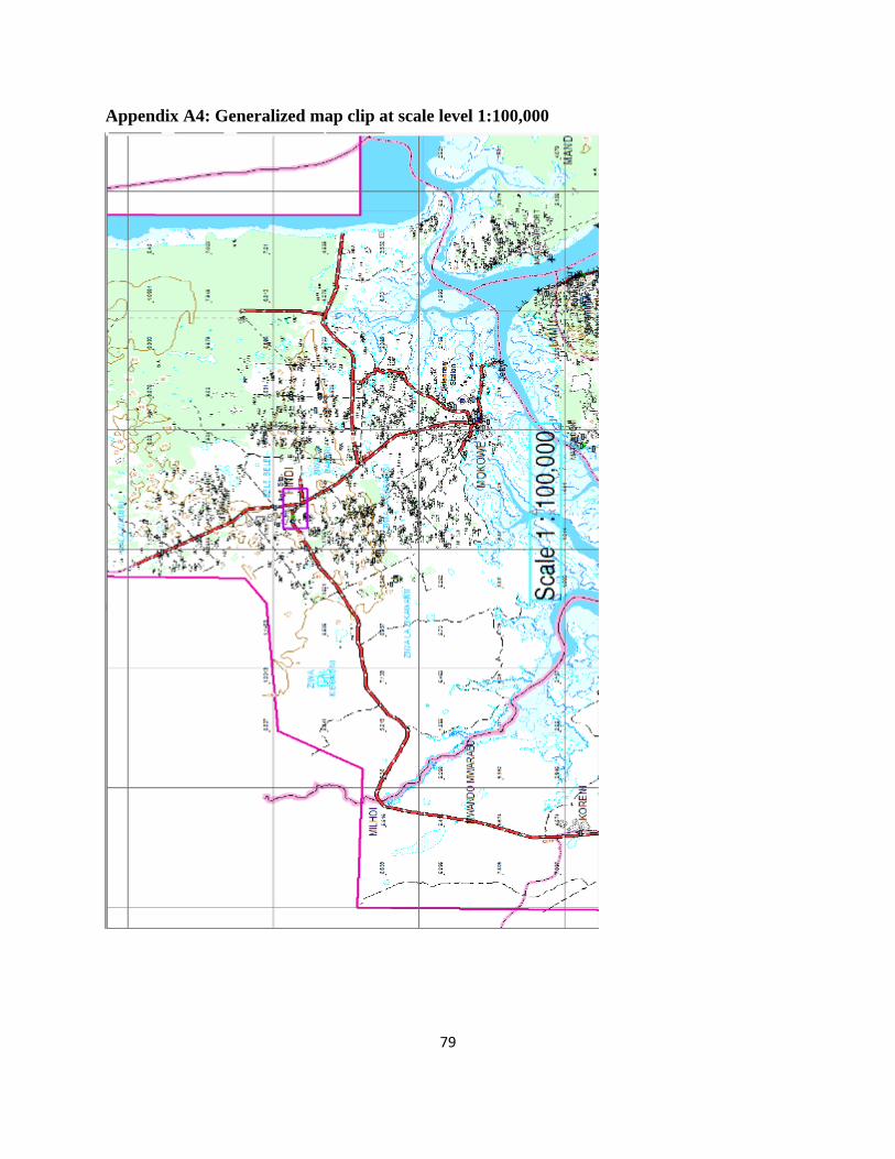
79
Appendix A4: Generalized map clip at scale level 1:100,000

80
Appendix B1 Symbols table scale 1:5,000 (base scale)

81
Appendix B2 :Symbols table scale 1:10,000

82
Appendix B3: Symbols table scale 1:50,000

83
Appendix B4: Symbols table scale 1:100,000


