3D Surface Modeling from Curves

aLaboratoire de Vision et Systemes NumeriquesDepartement de genie electrique et de genie informatique

Universite LavalSainte-Foy (Quebec), Canada G1K 7P4

Dragan Tubic a Patrick Hebert a Denis Laurendeau a

Abstract

Traditional approaches for surface reconstruction from range data require that theinput data be either range images or unorganized sets of points. With these meth-ods, range data acquired along curvilinear patterns cannot be used for surface recon-struction unless constraints are imposed on the shape of the patterns or on sensordisplacement. This paper presents a novel approach for reconstructing a surface froma set of arbitrary, unorganized and intersecting curves. A strategy for updating thereconstructed surface during data acquisition is described as well. Curves are accu-mulated in a volumetric structure in which a vector field is built and updated. Theinformation that is needed for efficient curve registration is also directly availablein the vector field. The proposed modeling approach combines surface reconstruc-tion and curve registration into a unified procedure. The algorithm implementingthe approach is of linear complexity with respect to the number of input curvesand makes it suitable for interactive modeling. Simulated data based on a set ofsix curvilinear patterns as well as data acquired with a range sensor are used toillustrate the various steps of the algorithm.

Keywords: 3D modeling, surface reconstruction, 3D curves, geometric fusion,curve registration, volumetric representation

1 Introduction

Three-dimensional modeling from 3D (range) data is the process of building a3D surface model of a measured object. Depending on the type of the sensor,the range data can be a set of unorganized points, surface curves or rangeimages (surface patches). In all cases however, range data acquired from asingle viewpoint is not sufficient to build a complete model; thus the 3D sen-sor or the object have to be moved in order to observe the whole surface.This creates redundancy in acquired data with respect to the resolution ofthe final model since, in general, it is practically not possible to observe the

Preprint submitted to Elsevier Science 26 February 2004

whole surface without observing some regions two or more times. When therange data is a set of surface patches, building a model consists in removingthis redundant data and reparameterizing the surface. This process is usuallyreferred to as geometric fusion. Building a model of a given resolution fromcurves or unorganized sets of points also requires removing redundant dataas well but in addition, surface reconstruction is necessary since curves andunorganized points do not represent a surface. Although the redundancy ofrange data might appear as a setback, it is however very useful in solvinganother problem, registration of multiple views.

Alignment, or registration of range data is required if the sensor position andorientation are not perfectly known for each viewpoint. That information isusually obtained by using an external positioning device but some sensors canalso estimate their position using features present in the observed scene [7].Since the estimate of sensor position is always inaccurate to some degree, therange data is not perfectly aligned once it is transformed into a common ref-erence frame. This sensor position error is referred to as the registration error.Note that in 3D modeling it is assumed that an approximate position of thesensor is known since the commonly used algorithms cannot handle arbitraryinitial positions. For this reason, registration is more correctly referred to aspose refinement in the context of 3D modeling. To align two views it is suf-ficient to identify at least three common points on each view and compute arigid transformation that aligns them. Selecting common points is referred toas matching and is usually based on the ICP (Iterated Closest Points) algo-rithm [2] while numerous variants and specific implementations exist. In thispaper, the process of three-dimensional modeling integrates geometric fusion,surface reconstruction and registration.

A very common type of range sensor acquires curvilinear measurements (sur-face profiles) on the surface of an object. Based on optical triangulation, thesesensors use a focused laser pattern projected on the surface and can providedense profiles robustly in a very short time frame. Although various laser pat-terns are available, methods for surface reconstruction from arbitrary curvesstill need to be developed. Currently, it is often assumed that profiles aregathered at regular intervals along a well defined path allowing neighbour-ing profiles to be grouped into a surface. The relative pose of each profile isassumed to be accurate. For hand-held sensors that collect profiles, it is notpossible to scan a surface along an exactly predefined scanning path. Thus,some methods have been proposed to build local surface patches from a rigidseries of profiles with known position but with only nearly regular scanningpaths [3,9,11,15]. There are still two problems with these methods. First, theonly type of surface curves that can be used are surface profiles. Second, al-though error in sensor positioning cannot be avoided during acquisition, it isnot possible to refine the pose for a single profile. This results in a loss of qual-ity of the model. The current alternative for low cost hand-held acquisition

2

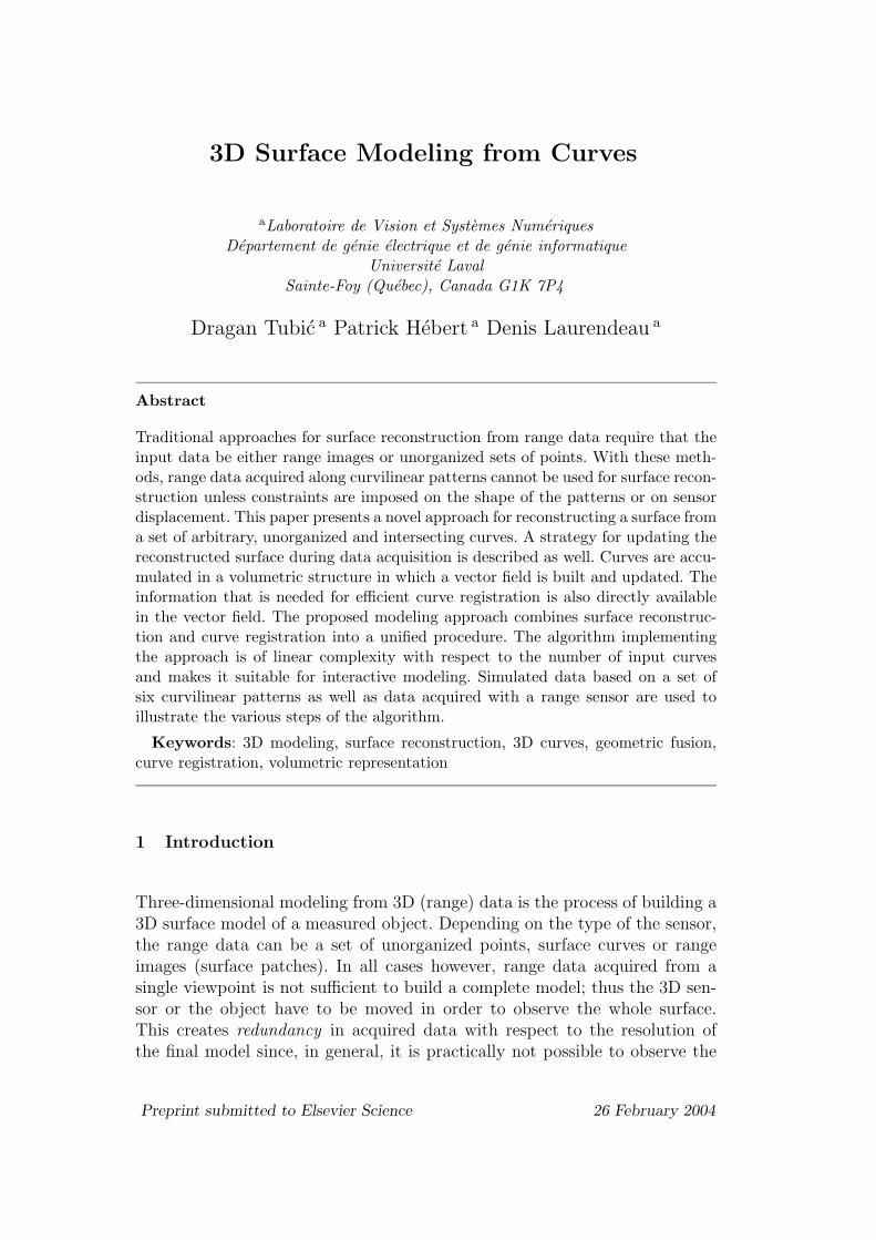
Fig. 1. Example of surface reconstruction from two curves.

is to collect range images [6,14] at the expense of losing robustness of lasersensors. In this paper, an approach is proposed for surface reconstruction offree-form objects from arbitrary curves as well as for the correction of the poseof each individual curve.

Surface curves contain more information about the measured surface than anunorganized set of points, namely tangents that can be exploited to improvethe quality of the reconstructed surface. A local estimate of the surface canbe obtained using tangents of intersecting curves. Later in this paper, it isexplained that for each point on the reconstructed surface, its surface normalis assessed from the tangents at the closest points on the neighbouring curves.Figure 1 illustrates the simplest case where a surface is reconstructed in theneighbourhood of two intersecting curves. Since the surface is approximated,the error of the reconstructed surface increases as the distance from the in-tersection increases. However, one can observe that the reconstructed surfacestill faithfully follows the shape of the original surface. This cannot be ac-complished by reducing curves to unorganized sets of points, i.e. by fitting aplane in the neighbourhood of a point (see also Figure 3). This improvementis particularly important in the regions of uneven sampling density such asthe example in Figure 1.

It is also shown that surface reconstruction can be performed efficiently usinga volumetric structure where the surface is incrementally recovered as new sur-face curves are scanned. Volumetric structures have been exploited for surfacereconstruction from range images or unordered sets of points [4,9,13,15,17]to reduce computational complexity and provide incremental reconstruction.These approaches use an implicit representation of the surface e.g. a scalarsigned distance field computed on a volumetric grid where the reconstructedsurface corresponds to the zero crossings of the field. The first contribution ofthis paper is to describe how such a volumetric representation can be builtdirectly from a set of measured curves using their tangents without any inter-

3

mediate surface representation. Furthermore, the computational complexitywith respect to the number of curves is linear and the reconstruction is in-cremental and order independent; thus no constraints are imposed on sensordisplacement. Any light pattern can be used to measure curves as long as thecurves intersect.

If one not only encodes the signed distance field in the volumetric structurebut also includes the direction towards the nearest zero crossing in each voxel,then matching (closest point) for a point can be obtained directly from thenearest voxel. We have developed this idea to provide near real-time registra-tion of range images [18]. The second main contribution in this paper is to stillmaintain the same linear complexity registration for surface curves by regis-tering them with the reconstructed surface. Another important aspect of ourapproach is a novel definition of distance measure that improves robustness ofregistration in the presence of noise.

Due to the shadow effects, some regions of the object are not measured duringthe acquisition of range data, resulting in holes in the final model. The objectthen has to be rescanned to complete the model in these regions. It is thusadvantageous to provide a partially reconstructed model in real-time to guidethe operator for the selection of the next best view that allows completion ofthe model with minimal acquisition time. The linear computational complexityof all modeling steps in the approach makes on-line surface reconstruction andregistration feasible.

The paper is organized as follows. The next section presents a summary ofexisting methods for surface reconstruction and registration. Sections 3.1 and3.2 describe the principle of surface reconstruction from curves, followed bysection 3.3 which explains a modification required to allow incremental re-construction. A novel definition of distance aimed at improving robustness ofregistration is presented in section 3.4. Section 3.5 exposes curve registration.The results presented in section 4 illustrate each aspect of the approach usingsimulated and real data.

2 Related Work

Reconstruction methods from range data (geometric fusion of multiple views)can be divided into two groups based on the representation of a surface: sur-face based approaches [16,19] and volumetric approaches [4,9,10,13,15]. In thispaper we concentrate on the latter group. Volumetric approaches to surfacereconstruction and fusion are based on implicit surface representation as asigned distance field. The surface itself is the zero-set of the scalar field. Inthe case of range images, this scalar field is used to merge multiple views by

4

n

t1

t2

n

(a) (b)

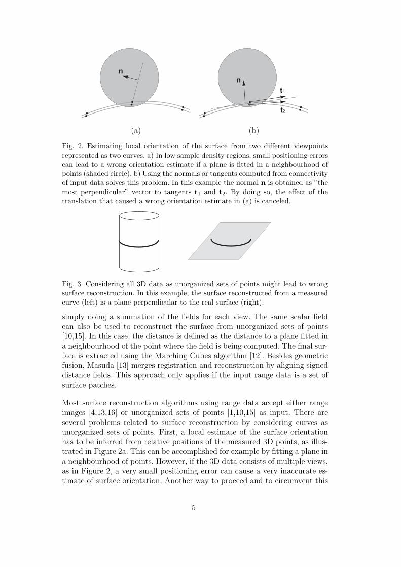
Fig. 2. Estimating local orientation of the surface from two different viewpointsrepresented as two curves. a) In low sample density regions, small positioning errorscan lead to a wrong orientation estimate if a plane is fitted in a neighbourhood ofpoints (shaded circle). b) Using the normals or tangents computed from connectivityof input data solves this problem. In this example the normal n is obtained as ”themost perpendicular” vector to tangents t1 and t2. By doing so, the effect of thetranslation that caused a wrong orientation estimate in (a) is canceled.

Fig. 3. Considering all 3D data as unorganized sets of points might lead to wrongsurface reconstruction. In this example, the surface reconstructed from a measuredcurve (left) is a plane perpendicular to the real surface (right).

simply doing a summation of the fields for each view. The same scalar fieldcan also be used to reconstruct the surface from unorganized sets of points[10,15]. In this case, the distance is defined as the distance to a plane fitted ina neighbourhood of the point where the field is being computed. The final sur-face is extracted using the Marching Cubes algorithm [12]. Besides geometricfusion, Masuda [13] merges registration and reconstruction by aligning signeddistance fields. This approach only applies if the input range data is a set ofsurface patches.

Most surface reconstruction algorithms using range data accept either rangeimages [4,13,16] or unorganized sets of points [1,10,15] as input. There areseveral problems related to surface reconstruction by considering curves asunorganized sets of points. First, a local estimate of the surface orientationhas to be inferred from relative positions of the measured 3D points, as illus-trated in Figure 2a. This can be accomplished for example by fitting a plane ina neighbourhood of points. However, if the 3D data consists of multiple views,as in Figure 2, a very small positioning error can cause a very inaccurate es-timate of surface orientation. Another way to proceed and to circumvent this

5

problem is to use additional information that is contained in the connectivityof points in curves and surface patches. For example, on a triangulated sur-face, the immediate neighbours for each point are known and can be used toestimate the surface normal at each point. In this case the surface orientationis estimated as the average of normals in a neighbourhood, see Figure 2b. Bydoing so, the effect of the registration error is much smaller than in the previ-ous case. Similarly, curve tangents can be used to improve reconstruction andreduce the effect of registration errors as explained later.

Another reason to use connectivity information in 3D data (tangents or nor-mals) is the ambiguity that leads to completely wrong surface reconstruction.One example of such an ambiguity is shown in Figure 3 where a single curveis measured on a cylindrical object. By considering this curve as an unorga-nized set of points, the reconstructed surface will inevitably be a plane thatcontains the curve and will be perpendicular to the real surface. The reasonfor this is that curves are dense sets of points but only along one dimension,i.e the distance between curves is not necessarily the same as the distancebetween neighbouring points within a single curve. This means that, for ex-ample, the surface shown in Figure 1 could not be reconstructed using surfacereconstruction algorithms from unorganized points since they generally as-sume a relatively uniform distribution of points over the surface. The methodproposed in this paper for surface reconstruction from curves eliminates thisproblem by using curve tangents to obtain a local estimate of the surface.

With the exception of [9], none of the proposed surface reconstruction meth-ods is applicable to the reconstruction from surface curves. Nevertheless, themethod proposed in [9] assumes that the input data is a set of surface profileswhich can be locally triangulated to produce a surface. Once the profiles aregrouped into a surface, it is considered as a surface patch so that a volumetricalgorithm can be used to reconstruct the surface. The triangulation step hasa negative impact on several aspects of modeling: the registration of individ-ual profiles cannot be performed, range data has to be acquired in regularsequences and the model cannot be constructed incrementally by integratinga single profile at a time. A post processing algorithm [3] for Hilton’s methodhas been proposed to improve the alignment of profiles as well as to optimizereconstructed surface. However, the algorithm [3] cannot register individualcurves and a specialized algorithm for this purpose is required.

Very little work has been reported on the subject of surface curve registration[8]. Although the stability of curve registration may have contributed to this,the main reason is the computational complexity of the registration process.The simultaneous registration based on the ICP (Iterated Closest Points) algo-rithm [2] is of complexity O(N2) with respect to the number of range images.If the same algorithm is applied for registration of surface curves, the com-plexity quickly becomes untractable since the number of curves required for

6

complete reconstruction of an object is at least an order of magnitude largerthan the equivalent number of range images and can easily reach several thou-sand curves.

A different approach for registration has been proposed in [17] where match-ing information is explicitly encoded in a volumetric grid in addition to thedistance field. Such a vector representation reduces computational complexityof registration and makes it linear with respect to the number of range imagesand the number of measured 3D points. Besides surface reconstruction, thispaper extends this approach to the registration of surface curves where thecomputational complexity is linear with respect to the number of curves.

3 Modeling using Range Curves

As reported in an earlier paper [17], the reconstructed surface is representedimplicitly as a vector field. Such a volumetric representation contains boththe reconstructed surface and its corresponding matching information in theform of direction and distance towards the reconstructed surface. The surfaceis represented as the zero-crossing of the signed norm of the field while the dis-tance and direction are represented by the field itself. Encoding both distanceand direction towards the surface allows one to find approximate closest points(required for registration) with linear complexity. Another advantage of thisvolumetric representation is that the reconstructed surface can be updatedincrementally. In the following, we describe how an implicit representation ofthe surface can be obtained from a set of non-parallel, intersecting surfacecurves.

3.1 Reconstruction from two intersecting curves

The main idea behind our approach is to perform reconstruction by approxi-mating the surface in the neighbourhood of the intersection points of surfacecurves. The reconstruction from two intersecting curves is first explained inorder to illustrate the principle on a simple case.

The reconstruction is based on a fundamental property of differential surfacesstating that all surface curves passing through some point have their tangentslocated in a plane tangent to the surface at the same point [5]. The mostimportant consequence of this property for our application is that the tangentplane to a surface at a given point can be computed using the vector productof the tangent to each curve at this point.

7

In theory, planes at the intersection points of surface curves could be usedto roughly approximate a surface. However, a faithful reconstruction wouldrequire too many intersections to be practical. In the presented approach, alimited number of intersections is used and a faithful surface representation isbuilt using tangent planes at these intersections and at points in their neigh-bourhoods.

The reconstructed surface S is implicitly represented as a vector field f : R3 →R3 where f(p) represents the direction and the distance to the closest pointpc on the surface S:

p + f(p) = pc ∈ S, (1)

such that

pc = argminq∈S

d(p,q), (2)

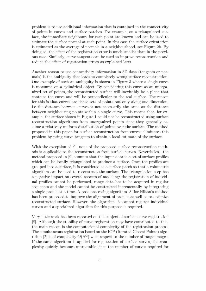
where d denotes a distance measure. In practice, the field f(p) is computedat points on a regular lattice (volumetric grid, see Figure 4) in the vicinityof a surface, usually referred to as its envelope. The envelope encloses latticepoints which are located at a distance to the surface smaller than a predefinedpositive value ε. An example of such an envelope for a curve is depicted inFigure 4.

To compute the implicit representation of the surface f(p) we start with twosurface curves α1 : U1 ⊂ R → R3 and α2 : U2 ⊂ R → R3 intersecting at asingle point pi = α1(U1)∩α2(U2) (see Figure 6). In the following it is assumedthat the surface is differentiable and that curves are parameterized by arclength. Now, for some lattice point (voxel) p, an approximation of the normaln to the tangent plane at the closest point of the surface is approximated asthe vector product of the tangents t1 and t2 at points p1 ∈ α1 and p2 ∈ α2

closest to p, i.e.

n = t1 × t2, (3)

where

p1 = argminq∈α1

d(p,q) = α1(u1), u1 ∈ U1,

p2 = argminq∈α2

d(p,q) = α2(u2), u2 ∈ U2,

t1 = α′1(u1),

t2 = α′2(u2) (4)

8

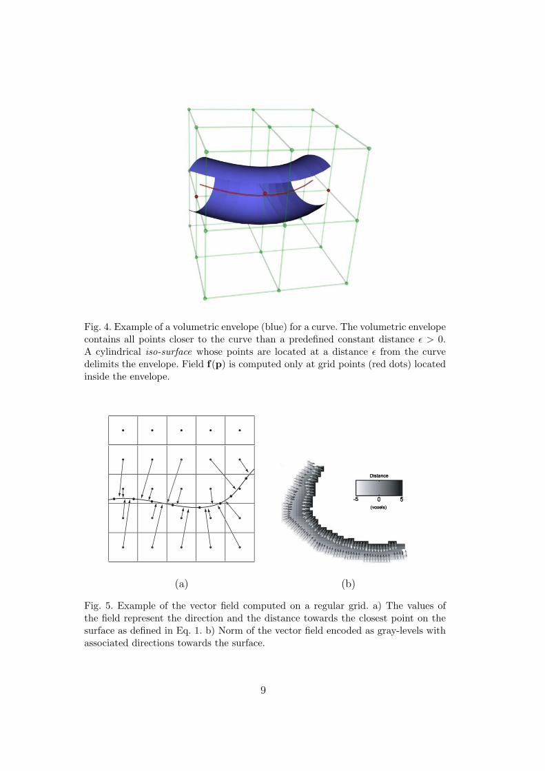
Fig. 4. Example of a volumetric envelope (blue) for a curve. The volumetric envelopecontains all points closer to the curve than a predefined constant distance ε > 0.A cylindrical iso-surface whose points are located at a distance ε from the curvedelimits the envelope. Field f(p) is computed only at grid points (red dots) locatedinside the envelope.

(a) (b)

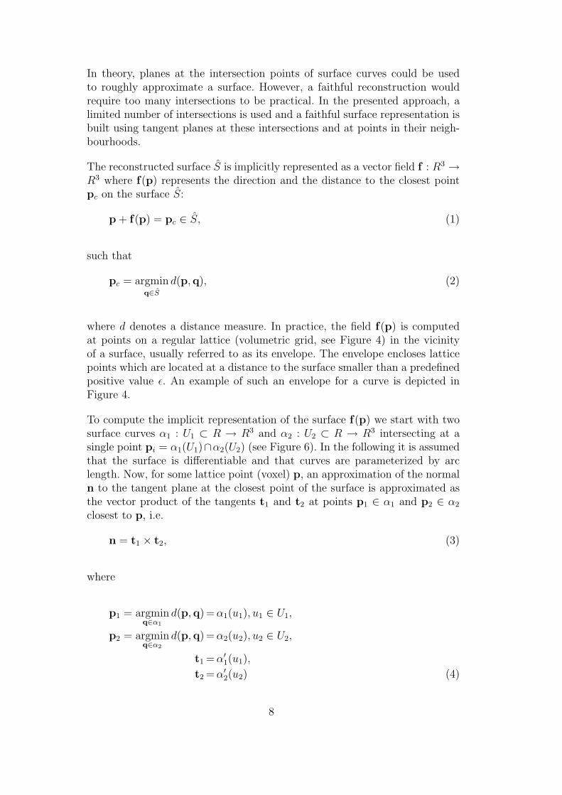
Fig. 5. Example of the vector field computed on a regular grid. a) The values ofthe field represent the direction and the distance towards the closest point on thesurface as defined in Eq. 1. b) Norm of the vector field encoded as gray-levels withassociated directions towards the surface.

9

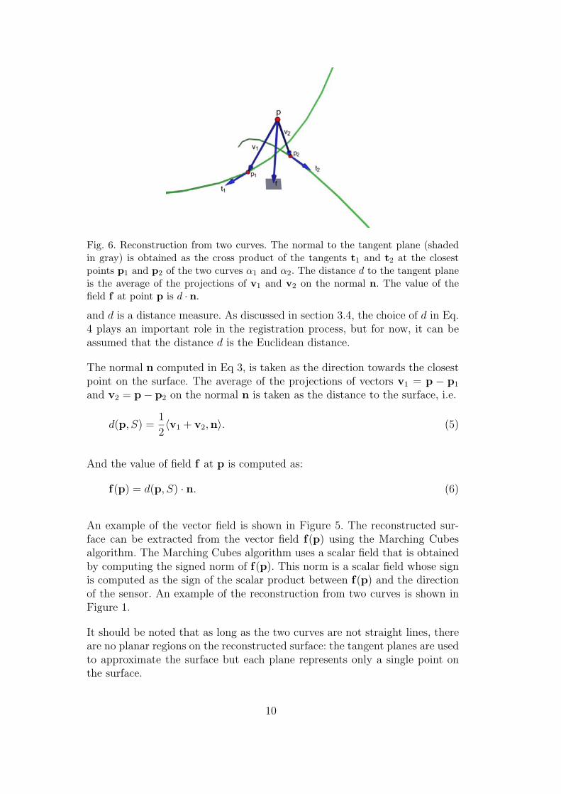
Fig. 6. Reconstruction from two curves. The normal to the tangent plane (shadedin gray) is obtained as the cross product of the tangents t1 and t2 at the closestpoints p1 and p2 of the two curves α1 and α2. The distance d to the tangent planeis the average of the projections of v1 and v2 on the normal n. The value of thefield f at point p is d · n.

and d is a distance measure. As discussed in section 3.4, the choice of d in Eq.4 plays an important role in the registration process, but for now, it can beassumed that the distance d is the Euclidean distance.

The normal n computed in Eq 3, is taken as the direction towards the closestpoint on the surface. The average of the projections of vectors v1 = p − p1

and v2 = p− p2 on the normal n is taken as the distance to the surface, i.e.

d(p, S) =1

2〈v1 + v2,n〉. (5)

And the value of field f at p is computed as:

f(p) = d(p, S) · n. (6)

An example of the vector field is shown in Figure 5. The reconstructed sur-face can be extracted from the vector field f(p) using the Marching Cubesalgorithm. The Marching Cubes algorithm uses a scalar field that is obtainedby computing the signed norm of f(p). This norm is a scalar field whose signis computed as the sign of the scalar product between f(p) and the directionof the sensor. An example of the reconstruction from two curves is shown inFigure 1.

It should be noted that as long as the two curves are not straight lines, thereare no planar regions on the reconstructed surface: the tangent planes are usedto approximate the surface but each plane represents only a single point onthe surface.

10

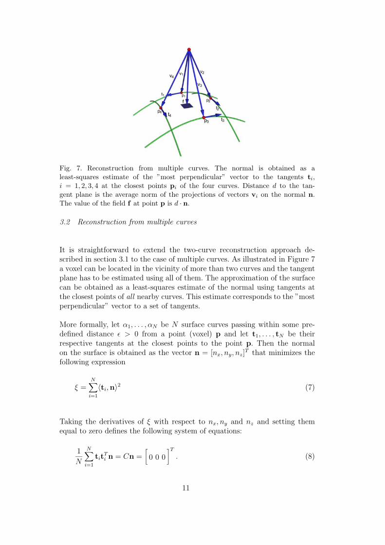
Fig. 7. Reconstruction from multiple curves. The normal is obtained as aleast-squares estimate of the ”most perpendicular” vector to the tangents ti,i = 1, 2, 3, 4 at the closest points pi of the four curves. Distance d to the tan-gent plane is the average norm of the projections of vectors vi on the normal n.The value of the field f at point p is d · n.

3.2 Reconstruction from multiple curves

It is straightforward to extend the two-curve reconstruction approach de-scribed in section 3.1 to the case of multiple curves. As illustrated in Figure 7a voxel can be located in the vicinity of more than two curves and the tangentplane has to be estimated using all of them. The approximation of the surfacecan be obtained as a least-squares estimate of the normal using tangents atthe closest points of all nearby curves. This estimate corresponds to the ”mostperpendicular” vector to a set of tangents.

More formally, let α1, . . . , αN be N surface curves passing within some pre-defined distance ε > 0 from a point (voxel) p and let t1, . . . , tN be theirrespective tangents at the closest points to the point p. Then the normalon the surface is obtained as the vector n = [nx, ny, nz]

T that minimizes thefollowing expression

ξ =N∑

i=1

〈ti,n〉2 (7)

Taking the derivatives of ξ with respect to nx, ny and nz and setting themequal to zero defines the following system of equations:

1

N

N∑i=1

titTi n = Cn =

[0 0 0

]T

. (8)

11

The solution for n is the eigenvector associated with the smallest eigenvalueof C which is the covariance matrix of the tangents.

The distance towards the surface is obtained as the average value of the pro-jected distance vectors on the estimated normal, i.e

d(p, S) =1

N

N∑i=1

〈pi − p,n〉 = 〈v,n〉 (9)

where pi is the closest point to p on curve αi. Finally, the value of the fieldat point p is:

f(p) = d(p, S) · n. (10)

In order to estimate the tangent plane to a surface at some point p, at least twonon-parallel tangents are needed to compute the matrix C at p since a singletangent does not define a plane. This condition can be verified by analyzingthe eigenvalues of matrix C: if two eigenvalues are zero, then only one tangent(or two or more parallel tangents) exists and the estimated normal at thatpoint is not used. This implies that the tangent plane cannot be estimatedfrom parallel curves, which makes the estimate less sensitive to registrationerrors (relative position of curves).

At the intersection points of noiseless and accurately positioned curves, alltangents are coplanar, hence one eigenvalue is always equal to zero and thetangents span a plane. Since, in our case, the surface is approximated in theneighbourhood of the intersection points, all three eigenvalues are generallylarger than zero. Also, if the tangents are estimated from noisy data, thethree eigenvalues may have similar values in which case the tangents spana cube and the estimate of the tangent plane is meaningless. To make surethat the estimated tangent plane is valid, an additional verification is madeon the eigenvalues. Let e1, e2 and e3 be the three eigenvalues such that e1 <e2 < e3. Since matrix C is normalized, the sum of the eigenvalues is alwaysequal to one i.e. e1 + e2 + e3 = 1 and fixed thresholds can be applied totest eigenvalues. It was confirmed empirically, that imposing the constraintse2 > 0.05 and e1 < 0.5e2 is enough to validate the estimated tangent plane.Imposing these constraints simply means that the tangents used to computeC must be approximately coplanar.

Since the size of the envelope determines how many curves influence the ma-trix C at each voxel, its role is important in the reconstruction process: Ifthe envelope chosen is too small with respect to the density of the curves,the reconstructed surface will either contain holes or it will appear as a setof patches located around intersection points. Two examples of a surface re-

12

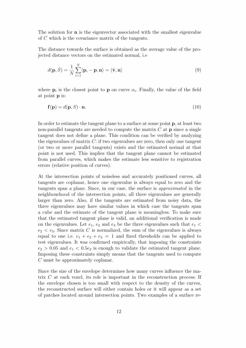
(a) (b)

Fig. 8. Surface reconstruction using a small envelope size with respect to the den-sity of range data. The shape of the reconstructed surface patches depends on theweighting function. a) Example of reconstruction using unweighted matrices Ci. b)Reconstruction using the weighting function defined in Eq. 11.

constructed with too small an envelope are shown in Figure 8. As illustratedin Figure 9, increasing the size of the envelope can solve this problem. Never-theless, increasing the size of the envelope also increases the execution time ofthe algorithm since the field is computed for a larger number of points. Moreimportantly, by increasing the size of the envelope, the number of tangentsused for estimating the tangent plane increases, as well as the distance to thecurves whose tangents are used. The consequence is a loss of details on thereconstructed surface since the least-squares estimation of the tangent planeacts as a low-pass filter. Having these constraints in mind, choosing the sizeof the envelope is thus a compromise. It is preferable to solve the problem ofsparse data by sampling the surface more densely. Since our approach aimsat interactive modeling where the reconstructed surface becomes available im-mediately after each curve has been acquired, it is easy to spot and resamplethe low-density regions during the acquisition of range data.

A single curve influences the field only at points located inside its envelopeand its influence drops to zero outside this envelope. Thus, the field computedfrom Eq. 10 is discontinuous over the edges of the envelope as well as thereconstructed surface. An example of such a reconstructed surface is shownin Figure 9. The solution to this problem is to weight the tangents using acontinuous function of distance that drops to zero at the edge of the enve-lope. Any decreasing, monotonic function can be used for this purpose. In ourexperiments the following function proved to be useful:

ω(d) = e−d2/σ2

. (11)

The value of σ is chosen equal to 1/2ε to make sure that the value of ωdrops close to zero outside the envelope. The weighting function also influencesthe shape of the reconstructed surface since it also acts as a low-pass filter

13

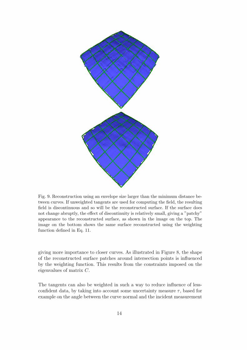
Fig. 9. Reconstruction using an envelope size larger than the minimum distance be-tween curves. If unweighted tangents are used for computing the field, the resultingfield is discontinuous and so will be the reconstructed surface. If the surface doesnot change abruptly, the effect of discontinuity is relatively small, giving a ”patchy”appearance to the reconstructed surface, as shown in the image on the top. Theimage on the bottom shows the same surface reconstructed using the weightingfunction defined in Eq. 11.

giving more importance to closer curves. As illustrated in Figure 8, the shapeof the reconstructed surface patches around intersection points is influencedby the weighting function. This results from the constraints imposed on theeigenvalues of matrix C.

The tangents can also be weighted in such a way to reduce influence of less-confident data, by taking into account some uncertainty measure τ , based forexample on the angle between the curve normal and the incident measurement

14

ray. After weighting with τ and ω, matrix C defined in Eq. 8 becomes

C =1∑N

i=1 τiωi

N∑i=1

τiωititTi . (12)

3.3 Incremental reconstruction

For the reconstruction approach described above, it was assumed that allthe data has been collected prior to reconstructing the surface. If the re-construction has to be performed online, then the field needs to be updatedincrementally by integrating a single measured curve at a time. However, theleast-squares estimate of the surface normal and, consequently, the vector field,cannot be computed incrementally. On the other hand, matrix C computed ateach voxel p is obtained as a sum and can therefore be updated incrementally.Let C(p) be the matrix C for the voxel p. Equation 12 can be rewritten as:

C(p) =1∑N

i=1 τiωi

N∑i=1

τiωiCi(p), (13)

where Ci(p) = titTi . During reconstruction, a matrix C(p) is associated with

each voxel and is updated after each curve αi has been acquired by summing itwith Ci(p). Matrix Ci(p) depends only on the curve αi and is computed usingthe tangent ti at the point pi on the curve that is closest to p. In addition tothe matrix C, the sum of distance vectors v is kept at each voxel as well (seeEq. 9). The value of the field f(p), defined in equations 9 and 10, is computedonly before the application of the surface using the Marching Cubes algorithmfor reconstruction or during registration.

3.4 Defining the distance and computing the vector field

So far the curves were considered as being continuous and noiseless. In prac-tice, the measured curves are represented as sets of line segments and cor-rupted by noise. The level of noise does not have a significant effect on thefunctionality of the algorithm with respect to the surface reconstruction pro-cess other than the quality of the reconstructed surface. The most importanteffect of noise is on the registration process, specifically on the matching step.As illustrated in Figure 15.a, the points with high noise level tend to attracta large number of correspondences. This slows down the registration processand makes it less accurate. To circumvent this problem, a new definition isadopted for distance d in Eq. 3 to replace the Euclidean distance.

15

To improve the robustness of matching, the direction towards the closest pointon the line segment has to be corrected while taking into account two impor-tant constraints: i) the distance field has to be continuous, ii) the positionof the measured 3D points should not be altered. The solution for this prob-lem is to filter and interpolate tangents over the line segments and to definethe distance using the filtered tangents. For the sake of clarity, the distancecomputation is first illustrated in 2D, the curve being contained in a plane.

A curve is considered as a linear interpolation of measured points {p1 . . .pN}represented as a set of line segments α = {l1, . . . , lN−1} where li = pipi+1.Except for end-points, the tangent at each measured point pi can be computedas follows:

ti =1

2

[pi−1 − pi

‖pi−1 − pi‖ +pi − pi+1

‖pi − pi+1‖ .]

(14)

The tangents ti are filtered with a filter Φ whose size is 2N + 1:

ti =i+N∑

k=i−N

tkΦ(k − i). (15)

For the experiments reported herein, a simple low-pass filter,

Φ(i) =

1/(2N + 1) if i ∈ [−N, . . . , N ] ,

0 otherwise(16)

was chosen.

The distance between some point p and the curve α is computed with respectto the closest line segment lc, i.e.

d(p, α) = d(p, lc),

lc = argminl∈α

d(p, l), (17)

where d denotes a distance measure. It is therefore sufficient to provide thedistance from a point to a line segment. The set of all points Π ⊂ R3 for whoma line segment lc is the closest, is called a fundamental cell associated withthe generator line segment lc. For the purpose of surface modeling, the fieldneeds to be calculated only within a relatively small distance ε > 0 from themeasured curve thus limiting the size of the cell to the set of points which arecloser than ε, i.e. inside the envelope. If d is the Euclidean distance then the

16

q1p

q2

ddd

n1nc

n2

p1 pc p2uc

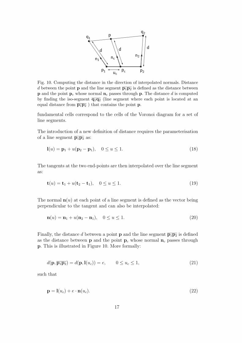
Fig. 10. Computing the distance in the direction of interpolated normals. Distanced between the point p and the line segment p1p2 is defined as the distance betweenp and the point pc whose normal nc passes through p. The distance d is computedby finding the iso-segment q1q2 (line segment where each point is located at anequal distance from p1p2 ) that contains the point p.

fundamental cells correspond to the cells of the Voronoi diagram for a set ofline segments.

The introduction of a new definition of distance requires the parameterisationof a line segment p1p2 as:

l(u) = p1 + u(p2 − p1), 0 ≤ u ≤ 1. (18)

The tangents at the two end-points are then interpolated over the line segmentas:

t(u) = t1 + u(t2 − t1), 0 ≤ u ≤ 1. (19)

The normal n(u) at each point of a line segment is defined as the vector beingperpendicular to the tangent and can also be interpolated:

n(u) = n1 + u(n2 − n1), 0 ≤ u ≤ 1. (20)

Finally, the distance d between a point p and the line segment p1p2 is definedas the distance between p and the point pc whose normal nc passes throughp. This is illustrated in Figure 10. More formally:

d(p,p1p2) = d(p, l(uc)) = e, 0 ≤ uc ≤ 1, (21)

such that

p = l(uc) + e · n(uc). (22)

17

n1

n2

p1 p2

pd1

d2

d2

d1

q''1

q''2

q'1

q'2

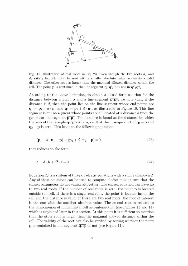
Fig. 11. Illustration of real roots in Eq. 23. Even though the two roots d1 andd2 satisfy Eq. 23, only the root with a smaller absolute value represents a validdistance. The other root is larger than the maximal allowed distance within thecell. The point p is contained in the line segment q′

1q′2 but not in q′′

1q′′2.

According to the above definition, to obtain a closed form solution for thedistance between a point p and a line segment p1p2, we note that, if thedistance is d, then the point lies on the line segment whose end-points areq1 = p1 + d · n1 and q2 = p2 + d · n2, as illustrated in Figure 10. This linesegment is an iso-segment whose points are all located at a distance d from thegenerator line segment p1p2. The distance is found as the distance for whichthe area of the triangle q1q2p is zero, i.e. that the cross-product of q1−p andq2 − p is zero. This leads to the following equation:

(p1 + d · n1 − p)× (p2 + d · n2 − p) = 0, (23)

that reduces to the form

a + d · b + d2 · c= 0. (24)

Equation 23 is a system of three quadratic equations with a single unknown d.Any of these equations can be used to compute d after making sure that thechosen parameters do not vanish altogether. The chosen equation can have upto two real roots. If the number of real roots is zero, the point p is locatedoutside the cell. If there is a single real root, the point is located inside thecell and the distance is valid. If there are two real roots, the root of interestis the one with the smallest absolute value. The second root is related tothe phenomenon of fundamental cell self-intersection (see Figures 11 and 14)which is explained later in this section. At this point it is sufficient to mentionthat the other root is larger than the maximal allowed distance within thecell. The validity of the root can also be verified by testing whether the pointp is contained in line segment q1q2 or not (see Figure 11).

18

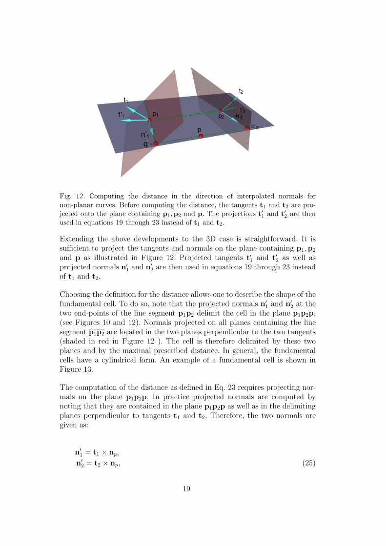
Fig. 12. Computing the distance in the direction of interpolated normals fornon-planar curves. Before computing the distance, the tangents t1 and t2 are pro-jected onto the plane containing p1,p2 and p. The projections t′1 and t′2 are thenused in equations 19 through 23 instead of t1 and t2.

Extending the above developments to the 3D case is straightforward. It issufficient to project the tangents and normals on the plane containing p1,p2

and p as illustrated in Figure 12. Projected tangents t′1 and t′2 as well asprojected normals n′

1 and n′2 are then used in equations 19 through 23 instead

of t1 and t2.

Choosing the definition for the distance allows one to describe the shape of thefundamental cell. To do so, note that the projected normals n′

1 and n′2 at the

two end-points of the line segment p1p2 delimit the cell in the plane p1p2p,(see Figures 10 and 12). Normals projected on all planes containing the linesegment p1p2 are located in the two planes perpendicular to the two tangents(shaded in red in Figure 12 ). The cell is therefore delimited by these twoplanes and by the maximal prescribed distance. In general, the fundamentalcells have a cylindrical form. An example of a fundamental cell is shown inFigure 13.

The computation of the distance as defined in Eq. 23 requires projecting nor-mals on the plane p1p2p. In practice projected normals are computed bynoting that they are contained in the plane p1p2p as well as in the delimitingplanes perpendicular to tangents t1 and t2. Therefore, the two normals aregiven as:

n′1 = t1 × np,

n′2 = t2 × np, (25)

19

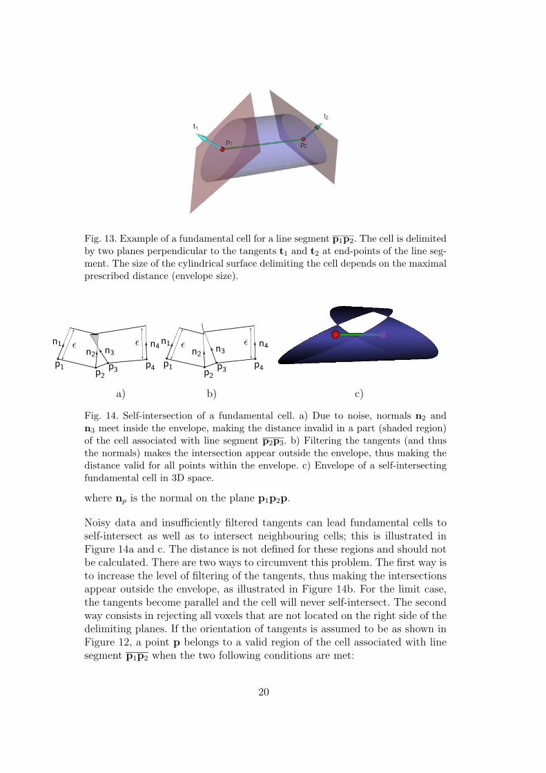
Fig. 13. Example of a fundamental cell for a line segment p1p2. The cell is delimitedby two planes perpendicular to the tangents t1 and t2 at end-points of the line seg-ment. The size of the cylindrical surface delimiting the cell depends on the maximalprescribed distance (envelope size).

p1p2

p3p4

εεn1n2 n3

n4

p1p2

p3p4

εεn1n2

n3n4

a) b) c)

Fig. 14. Self-intersection of a fundamental cell. a) Due to noise, normals n2 andn3 meet inside the envelope, making the distance invalid in a part (shaded region)of the cell associated with line segment p2p3. b) Filtering the tangents (and thusthe normals) makes the intersection appear outside the envelope, thus making thedistance valid for all points within the envelope. c) Envelope of a self-intersectingfundamental cell in 3D space.

where np is the normal on the plane p1p2p.

Noisy data and insufficiently filtered tangents can lead fundamental cells toself-intersect as well as to intersect neighbouring cells; this is illustrated inFigure 14a and c. The distance is not defined for these regions and should notbe calculated. There are two ways to circumvent this problem. The first way isto increase the level of filtering of the tangents, thus making the intersectionsappear outside the envelope, as illustrated in Figure 14b. For the limit case,the tangents become parallel and the cell will never self-intersect. The secondway consists in rejecting all voxels that are not located on the right side of thedelimiting planes. If the orientation of tangents is assumed to be as shown inFigure 12, a point p belongs to a valid region of the cell associated with linesegment p1p2 when the two following conditions are met:

20

〈p1 − p, t1〉≤ 0,

〈p2 − p,−t2〉≤ 0, (26)

since the tangents are normal to delimiting planes.

Equation 21 is valid only inside the fundamental cell of a line segment. Priorto computing the distance to the curve at some point p, one has to find towhich cell the point p belongs. This is a tedious task that can be avoided byinverting the process and by rather finding all voxels falling inside each cellseparately. By doing so, the complexity of field computation is linear withrespect to the number of line segments (measured points).

Computing the field for a cell reduces therefore to a simple two-step process.First, the bounding box of a cell is computed. The two defining corners ofthe bounding box can be obtained as minimum and maximum values of p1 +ε,p1 − ε,p2 + ε,p2 − ε. Then, for all grid points located inside the boundingbox, it is verified whether they are located between the two delimiting planesas in Eq. 26. If it is so, the distance is computed and accepted if it is smallerthan the maximum allowed distance.

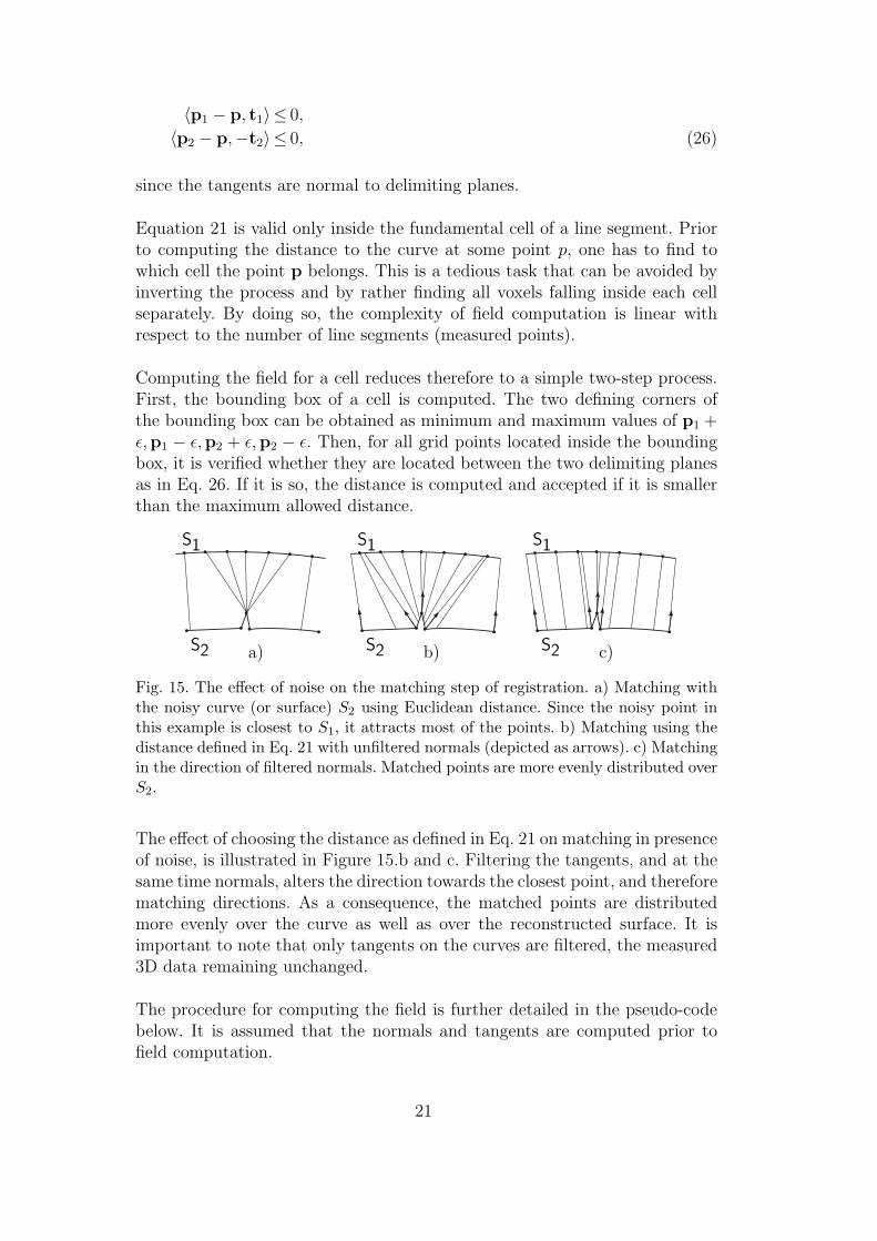
a) b) c)

S1S1S1

S2S2S2

Fig. 15. The effect of noise on the matching step of registration. a) Matching withthe noisy curve (or surface) S2 using Euclidean distance. Since the noisy point inthis example is closest to S1, it attracts most of the points. b) Matching using thedistance defined in Eq. 21 with unfiltered normals (depicted as arrows). c) Matchingin the direction of filtered normals. Matched points are more evenly distributed overS2.

The effect of choosing the distance as defined in Eq. 21 on matching in presenceof noise, is illustrated in Figure 15.b and c. Filtering the tangents, and at thesame time normals, alters the direction towards the closest point, and thereforematching directions. As a consequence, the matched points are distributedmore evenly over the curve as well as over the reconstructed surface. It isimportant to note that only tangents on the curves are filtered, the measured3D data remaining unchanged.

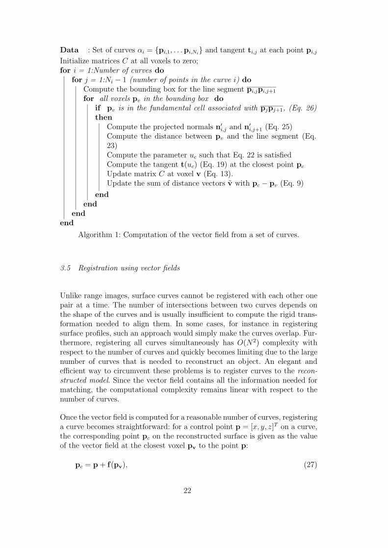
The procedure for computing the field is further detailed in the pseudo-codebelow. It is assumed that the normals and tangents are computed prior tofield computation.

21

Data : Set of curves αi = {pi,1, . . .pi,Ni} and tangent ti,j at each point pi,j

Initialize matrices C at all voxels to zero;for i = 1:Number of curves do

for j = 1:Ni − 1 (number of points in the curve i) doCompute the bounding box for the line segment pi,jpi,j+1

for all voxels pv in the bounding box doif pv is in the fundamental cell associated with pjpj+1, (Eq. 26)then

Compute the projected normals n′i,j and n′

i,j+1 (Eq. 25)Compute the distance between pv and the line segment (Eq.23)Compute the parameter uc such that Eq. 22 is satisfiedCompute the tangent t(uc) (Eq. 19) at the closest point pc

Update matrix C at voxel v (Eq. 13).Update the sum of distance vectors v with pc − pv (Eq. 9)

endend

endend

Algorithm 1: Computation of the vector field from a set of curves.

3.5 Registration using vector fields

Unlike range images, surface curves cannot be registered with each other onepair at a time. The number of intersections between two curves depends onthe shape of the curves and is usually insufficient to compute the rigid trans-formation needed to align them. In some cases, for instance in registeringsurface profiles, such an approach would simply make the curves overlap. Fur-thermore, registering all curves simultaneously has O(N2) complexity withrespect to the number of curves and quickly becomes limiting due to the largenumber of curves that is needed to reconstruct an object. An elegant andefficient way to circumvent these problems is to register curves to the recon-structed model. Since the vector field contains all the information needed formatching, the computational complexity remains linear with respect to thenumber of curves.

Once the vector field is computed for a reasonable number of curves, registeringa curve becomes straightforward: for a control point p = [x, y, z]T on a curve,the corresponding point pc on the reconstructed surface is given as the valueof the vector field at the closest voxel pv to the point p:

pc = p + f(pv), (27)

22

pc

pv

p

pv+F(pv)

f(pv)

∆

∆

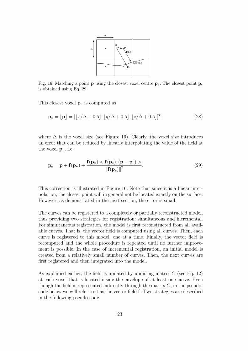
Fig. 16. Matching a point p using the closest voxel centre pv. The closest point pc

is obtained using Eq. 29.

This closest voxel pv is computed as

pv = p = [x/∆ + 0.5, y/∆ + 0.5, z/∆ + 0.5]T , (28)

where ∆ is the voxel size (see Figure 16). Clearly, the voxel size introducesan error that can be reduced by linearly interpolating the value of the field atthe voxel pv, i.e.

pc = p + f(pv) +f(pv) < f(pv), (p− pv) >

‖f(pv)‖2. (29)

This correction is illustrated in Figure 16. Note that since it is a linear inter-polation, the closest point will in general not be located exactly on the surface.However, as demonstrated in the next section, the error is small.

The curves can be registered to a completely or partially reconstructed model,thus providing two strategies for registration: simultaneous and incremental.For simultaneous registration, the model is first reconstructed from all avail-able curves. That is, the vector field is computed using all curves. Then, eachcurve is registered to this model, one at a time. Finally, the vector field isrecomputed and the whole procedure is repeated until no further improve-ment is possible. In the case of incremental registration, an initial model iscreated from a relatively small number of curves. Then, the next curves arefirst registered and then integrated into the model.

As explained earlier, the field is updated by updating matrix C (see Eq. 12)at each voxel that is located inside the envelope of at least one curve. Eventhough the field is represented indirectly through the matrix C, in the pseudo-code below we will refer to it as the vector field f . Two strategies are describedin the following pseudo-code.

23

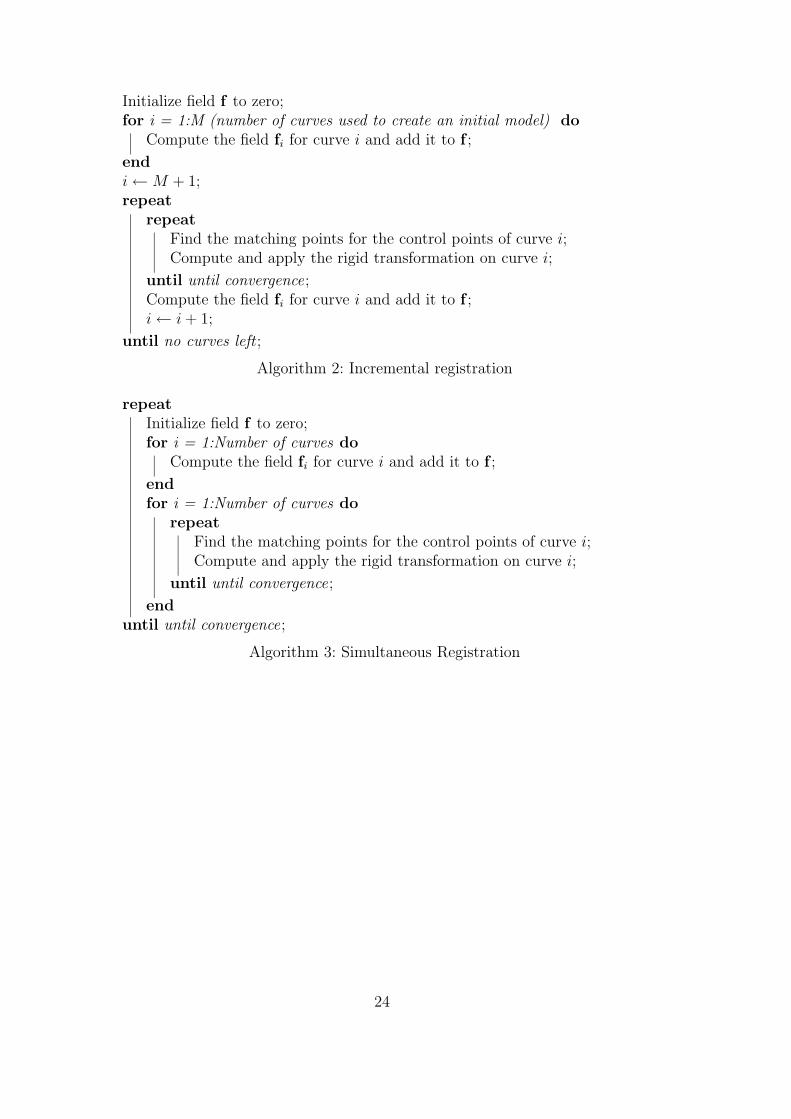
Initialize field f to zero;for i = 1:M (number of curves used to create an initial model) do

Compute the field fi for curve i and add it to f ;

endi←M + 1;repeat

repeatFind the matching points for the control points of curve i;Compute and apply the rigid transformation on curve i;

until until convergence;Compute the field fi for curve i and add it to f ;i← i + 1;

until no curves left ;

Algorithm 2: Incremental registration

repeatInitialize field f to zero;for i = 1:Number of curves do

Compute the field fi for curve i and add it to f ;

endfor i = 1:Number of curves do

repeatFind the matching points for the control points of curve i;Compute and apply the rigid transformation on curve i;

until until convergence;

enduntil until convergence;

Algorithm 3: Simultaneous Registration

24

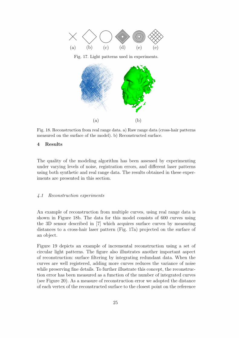
(a) (b) (c) (d) (e)(e)

Fig. 17. Light patterns used in experiments.

(a) (b)

Fig. 18. Reconstruction from real range data. a) Raw range data (cross-hair patternsmeasured on the surface of the model). b) Reconstructed surface.

4 Results

The quality of the modeling algorithm has been assessed by experimentingunder varying levels of noise, registration errors, and different laser patternsusing both synthetic and real range data. The results obtained in these exper-iments are presented in this section.

4.1 Reconstruction experiments

An example of reconstruction from multiple curves, using real range data isshown in Figure 18b. The data for this model consists of 600 curves usingthe 3D sensor described in [7] which acquires surface curves by measuringdistances to a cross-hair laser pattern (Fig. 17a) projected on the surface ofan object.

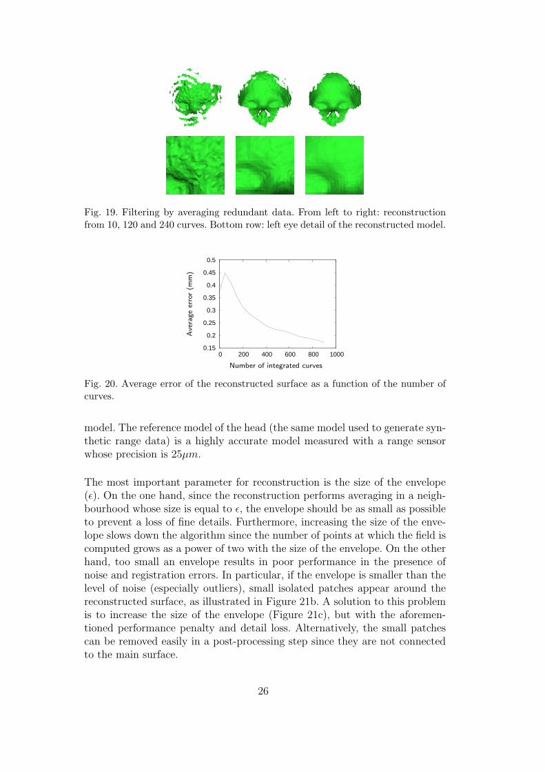
Figure 19 depicts an example of incremental reconstruction using a set ofcircular light patterns. The figure also illustrates another important aspectof reconstruction: surface filtering by integrating redundant data. When thecurves are well registered, adding more curves reduces the variance of noisewhile preserving fine details. To further illustrate this concept, the reconstruc-tion error has been measured as a function of the number of integrated curves(see Figure 20). As a measure of reconstruction error we adopted the distanceof each vertex of the reconstructed surface to the closest point on the reference

25

Fig. 19. Filtering by averaging redundant data. From left to right: reconstructionfrom 10, 120 and 240 curves. Bottom row: left eye detail of the reconstructed model.

0.15

0.2

0.25

0.3

0.35

0.4

0.45

0.5

0 200 400 600 800 1000

Ave

rage

erro

r(m

m)

Number of integrated curves

Fig. 20. Average error of the reconstructed surface as a function of the number ofcurves.

model. The reference model of the head (the same model used to generate syn-thetic range data) is a highly accurate model measured with a range sensorwhose precision is 25µm.

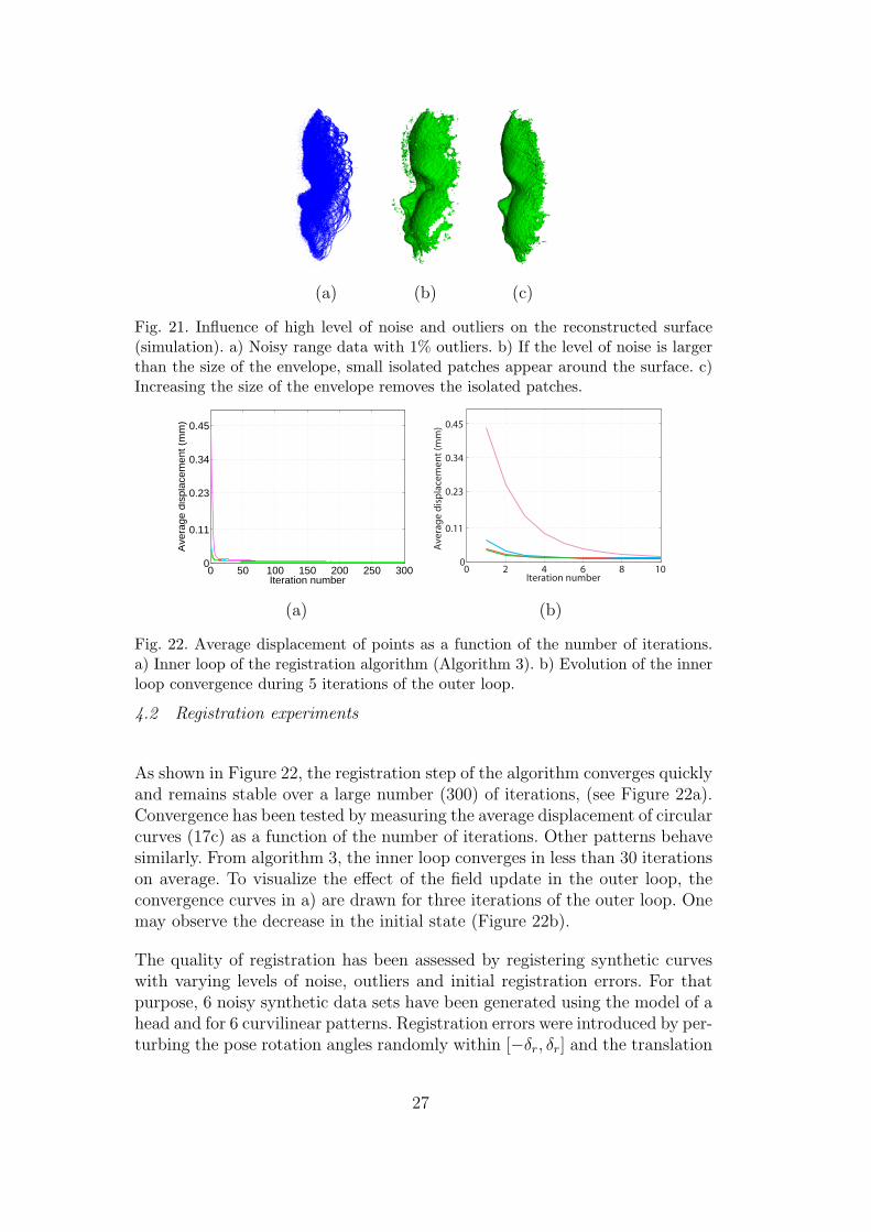
The most important parameter for reconstruction is the size of the envelope(ε). On the one hand, since the reconstruction performs averaging in a neigh-bourhood whose size is equal to ε, the envelope should be as small as possibleto prevent a loss of fine details. Furthermore, increasing the size of the enve-lope slows down the algorithm since the number of points at which the field iscomputed grows as a power of two with the size of the envelope. On the otherhand, too small an envelope results in poor performance in the presence ofnoise and registration errors. In particular, if the envelope is smaller than thelevel of noise (especially outliers), small isolated patches appear around thereconstructed surface, as illustrated in Figure 21b. A solution to this problemis to increase the size of the envelope (Figure 21c), but with the aforemen-tioned performance penalty and detail loss. Alternatively, the small patchescan be removed easily in a post-processing step since they are not connectedto the main surface.

26

(a) (b) (c)

Fig. 21. Influence of high level of noise and outliers on the reconstructed surface(simulation). a) Noisy range data with 1% outliers. b) If the level of noise is largerthan the size of the envelope, small isolated patches appear around the surface. c)Increasing the size of the envelope removes the isolated patches.

0 50 100 150 200 250 3000

0.11

0.23

0.34

0.45

Iteration number

Ave

rage

dis

plac

emen

t (m

m)

0 2 4 6 8 100

0.11

0.23

0.34

0.45A

vera

ge d

ispl

acem

ent (

mm

)

Iteration number

(a) (b)

Fig. 22. Average displacement of points as a function of the number of iterations.a) Inner loop of the registration algorithm (Algorithm 3). b) Evolution of the innerloop convergence during 5 iterations of the outer loop.

4.2 Registration experiments

As shown in Figure 22, the registration step of the algorithm converges quicklyand remains stable over a large number (300) of iterations, (see Figure 22a).Convergence has been tested by measuring the average displacement of circularcurves (17c) as a function of the number of iterations. Other patterns behavesimilarly. From algorithm 3, the inner loop converges in less than 30 iterationson average. To visualize the effect of the field update in the outer loop, theconvergence curves in a) are drawn for three iterations of the outer loop. Onemay observe the decrease in the initial state (Figure 22b).

The quality of registration has been assessed by registering synthetic curveswith varying levels of noise, outliers and initial registration errors. For thatpurpose, 6 noisy synthetic data sets have been generated using the model of ahead and for 6 curvilinear patterns. Registration errors were introduced by per-turbing the pose rotation angles randomly within [−δr, δr] and the translation

27

0.00 0.36 0.72 1.08 1.44

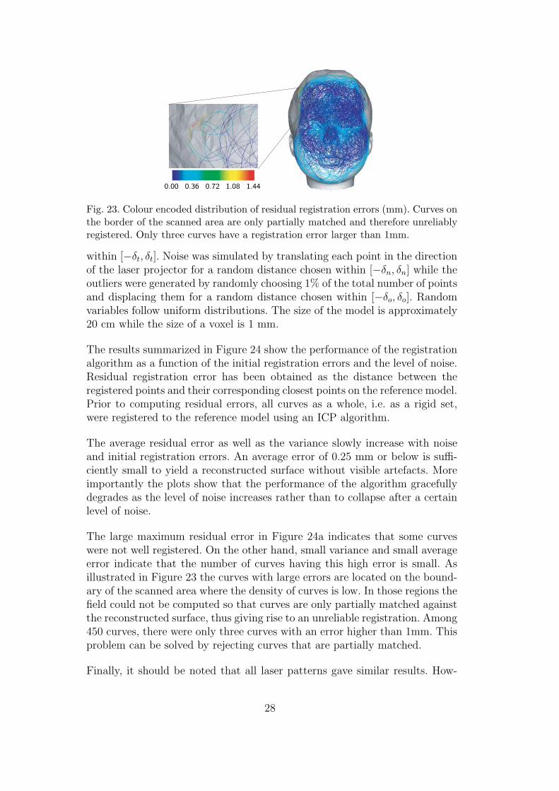
Fig. 23. Colour encoded distribution of residual registration errors (mm). Curves onthe border of the scanned area are only partially matched and therefore unreliablyregistered. Only three curves have a registration error larger than 1mm.

within [−δt, δt]. Noise was simulated by translating each point in the directionof the laser projector for a random distance chosen within [−δn, δn] while theoutliers were generated by randomly choosing 1% of the total number of pointsand displacing them for a random distance chosen within [−δo, δo]. Randomvariables follow uniform distributions. The size of the model is approximately20 cm while the size of a voxel is 1 mm.

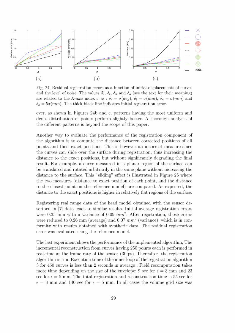
The results summarized in Figure 24 show the performance of the registrationalgorithm as a function of the initial registration errors and the level of noise.Residual registration error has been obtained as the distance between theregistered points and their corresponding closest points on the reference model.Prior to computing residual errors, all curves as a whole, i.e. as a rigid set,were registered to the reference model using an ICP algorithm.

The average residual error as well as the variance slowly increase with noiseand initial registration errors. An average error of 0.25 mm or below is suffi-ciently small to yield a reconstructed surface without visible artefacts. Moreimportantly the plots show that the performance of the algorithm gracefullydegrades as the level of noise increases rather than to collapse after a certainlevel of noise.

The large maximum residual error in Figure 24a indicates that some curveswere not well registered. On the other hand, small variance and small averageerror indicate that the number of curves having this high error is small. Asillustrated in Figure 23 the curves with large errors are located on the bound-ary of the scanned area where the density of curves is low. In those regions thefield could not be computed so that curves are only partially matched againstthe reconstructed surface, thus giving rise to an unreliable registration. Among450 curves, there were only three curves with an error higher than 1mm. Thisproblem can be solved by rejecting curves that are partially matched.

Finally, it should be noted that all laser patterns gave similar results. How-

28

0 0.5 1 1.5 20

2.5

5

7.5

10

Max

imal

err

or (

mm

)

σ

0 0.5 1 1.5 20

0.25

0.5

0.75

1

Ave

rage

err

or (

mm

)

σ

0 0.5 1 1.5 20

0.11

0.22

0.33

0.44

Var

ianc

e (m

m)

σinitial

(a) (b) (c)

Fig. 24. Residual registration errors as a function of initial displacements of curvesand the level of noise. The values δr, δt, δn and δo (see the text for their meaning)are related to the X-axis index σ as : δr = σ(deg), δt = σ(mm), δn = σ(mm) andδo = 5σ(mm). The thick black line indicates initial registration error.

ever, as shown in Figures 24b and c, patterns having the most uniform anddense distribution of points perform slightly better. A thorough analysis ofthe different patterns is beyond the scope of this paper.

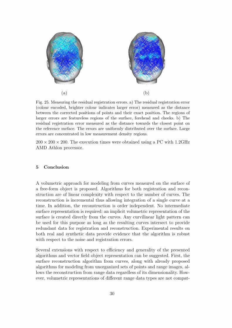
Another way to evaluate the performance of the registration component ofthe algorithm is to compute the distance between corrected positions of allpoints and their exact positions. This is however an incorrect measure sincethe curves can slide over the surface during registration, thus increasing thedistance to the exact positions, but without significantly degrading the finalresult. For example, a curve measured in a planar region of the surface canbe translated and rotated arbitrarily in the same plane without increasing thedistance to the surface. This ”sliding” effect is illustrated in Figure 25 wherethe two measures (distance to exact position of each point, and the distanceto the closest point on the reference model) are compared. As expected, thedistance to the exact positions is higher in relatively flat regions of the surface.

Registering real range data of the head model obtained with the sensor de-scribed in [7] data leads to similar results. Initial average registration errorswere 0.35 mm with a variance of 0.09 mm2. After registration, those errorswere reduced to 0.26 mm (average) and 0.07 mm2 (variance), which is in con-formity with results obtained with synthetic data. The residual registrationerror was evaluated using the reference model.

The last experiment shows the performance of the implemented algorithm. Theincremental reconstruction from curves having 250 points each is performed inreal-time at the frame rate of the sensor (30fps). Thereafter, the registrationalgorithm is run. Execution time of the inner loop of the registration algorithm3 for 450 curves is less than 2 seconds in average . Field recomputation takesmore time depending on the size of the envelope: 9 sec for ε = 3 mm and 23sec for ε = 5 mm. The total registration and reconstruction time is 55 sec forε = 3 mm and 140 sec for ε = 5 mm. In all cases the volume grid size was

29

(a) (b)

Fig. 25. Measuring the residual registration errors. a) The residual registration error(colour encoded, brighter colour indicates larger error) measured as the distancebetween the corrected positions of points and their exact position. The regions oflarger errors are featureless regions of the surface, forehead and cheeks. b) Theresidual registration error measured as the distance towards the closest point onthe reference surface. The errors are uniformly distributed over the surface. Largeerrors are concentrated in low measurement density regions.

200× 200× 200. The execution times were obtained using a PC with 1.2GHzAMD Athlon processor.

5 Conclusion

A volumetric approach for modeling from curves measured on the surface ofa free-form object is proposed. Algorithms for both registration and recon-struction are of linear complexity with respect to the number of curves. Thereconstruction is incremental thus allowing integration of a single curve at atime. In addition, the reconstruction is order independent. No intermediatesurface representation is required: an implicit volumetric representation of thesurface is created directly from the curves. Any curvilinear light pattern canbe used for this purpose as long as the resulting curves intersect to provideredundant data for registration and reconstruction. Experimental results onboth real and synthetic data provide evidence that the algorithm is robustwith respect to the noise and registration errors.

Several extensions with respect to efficiency and generality of the presentedalgorithms and vector field object representation can be suggested. First, thesurface reconstruction algorithm from curves, along with already proposedalgorithms for modeling from unorganized sets of points and range images, al-lows the reconstruction from range data regardless of its dimensionality. How-ever, volumetric representations of different range data types are not compat-

30

ible; this means that the created volumetric representation, say, from rangeimages cannot be updated with a set of curves or a set of points and viceversa. Unifying the volumetric representation for all types of range data wouldgreatly simplify the modeling process since it would allow mixing of range dataacquired with different range sensors. For example, an object could be scannedusing a range image sensor that provides 3D images while filling the hard toreach areas with a hand-held sensor that acquires surface curves.

Another important aspect of a modeling algorithm is the efficient use of com-puter resources. With respect to computational complexity, the presented al-gorithm is very efficient, having linear complexity, but the price to pay is avery inefficient use of computer memory. Even though already proposed com-pression schemes such as run length encoding or hash tables can be used toreduce memory requirements, it is still not as efficient as surface based rep-resentations since these methods encode only occupancy of voxels regardlessof the geometry of the object. We do believe that compression of volumetricdata based on the geometry of the object is possible and it will be, along withthe aforementioned problem of unified representation, the object of our futurework.

References

[1] M. Alexa, J. Behr, D. Cohen-Or, S. Fleishman, D. Levin, and C. T. Silva. Pointset surfaces. IEEE Visualization 2001, pages 21–28, October 2001.

[2] P. Besl and N. McKay. A method for registration of 3-d shapes. IEEETransactions on Pattern Analysis and Machine Intelligence, 14(2):239–256,February 1992.

[3] S. J. Cunnington and A. J. Stoddart. Self-calibrating surface reconstruction forthe modelmaker. In BMVC’98 proceedings, volume 2, pages 790–799, 1998.

[4] B. Curless and M. Levoy. A volumetric method for building complex modelsfrom range images. In SIGGRAPH ’96 Conference Proceedings, pages 303–312,August 1996.

[5] M. P. do Carmo. Differential Geometry of Curves and Surfaces. Prentice-Hall,1976. 503 pages.

[6] O. Hall-Holt and S. Rusinkiewicz. Stripe boundary codes for real-timestructured-light range scanning of moving objects. In Proceedings of ICCV2001, pages II: 359–366, 2001.

[7] P. Hebert. A self-referenced hand-held range sensor. In Proceedings of the ThirdInternational Conference on 3D Digital Imaging and Modeling (3DIM), pages5–11, May 2001.

31

[8] P. Hebert and M. Rioux. A self-referenced hand-held range sensor. InProceedings of SPIE: Three-Dimensional Image Capture and Applications, TheInternational Society for Optical Engineering, volume 3313, pages 2–13, January1998.

[9] A. Hilton and J. Illingworth. Geometric fusion for a hand-held 3d sensor.Machine vision and applications, 12:44–51, 2000.

[10] H. Hoppe, T. DeRose, T. Duchamp, J. McDonald, and W. Stuetzle. Surfacereconstruction from unorganized points. In Computer Graphics (SIGGRAPH’92 Proceedings), volume 26, pages 71–78, July 1992.

[11] J. Kofman and G. K. Knopf. Registration and integration of narrow andspatiotemporally-dense range views. In Proceedings of SPIE, Vision GeometryVII, volume 3454, pages 99–109, July 1998.

[12] W. E. Lorensen and H. E. Cline. Marching cubes: A high resolution 3D surfaceconstruction algorithm. SIGGRAPH ’87 Conference Proceedings, 21(4):163–169, 1987.

[13] T. Masuda. Object shape modeling from multiple range images by matchingsigned distance fields. In Proceedings of First International Symposium on 3Ddata Processing Visualization and Transmission (3DPVT), volume 1, pages439–448, June 2002.

[14] M. Proesmans, L. Van Gool, and F. Defoort. Reading between the lines - amethod for extracting dynamic 3d with texture. In Proceedings of ICCV 1998,pages 1081–1086, 1998.

[15] G. Roth and E. Wibowo. An efficient volumetric method for building closedtriangular meshes from 3-d image and point data. In W. Davis, M. Mantei, andV. Klassen, editors, Graphics Interface, pages 173–180, May 1997.

[16] M. Soucy and D. Laurendeau. A general surface approach to the integrationof a set of range views. IEEE Transactions on Pattern Analysis and MachineIntelligence, 17(4):344–358, 1995.

[17] D. Tubic, P. Hebert, and D. Laurendeau. A volumetric approach for interactive3d modeling. In Proceedings of 3DPVT, volume 1, pages 150–158, June 2002.

[18] D. Tubic, P. Hebert, and D. Laurendeau. A volumetric approach for interactive3d modeling. Computer Vision and Image Understanding, 92:56–77, 2003.

[19] G. Turk and M. Levoy. Zippered polygon meshes from range images.SIGGRAPH ’94 Conference Proceedings, 26:311–318, 1994.

32