Page 1
105
5 WORKING CAPITAL MANAGEMENT
5.1 INTRODUCTION
In working capital management, firms are employing more sophisticated
collection and disbursement systems. Maintaining appropriate cash balances or
inventory levels involves managing flows. Inefficient use of cash and materials
ultimately reduces the firm’s profitability. The C2C cycle time attempts to measure
the time elapsed between paying suppliers for material and getting paid by customers.
C2C cycle time is a unique financial performance metric that indicates how well an
entity is managing its working capital.
In integrated SCM, the problem arises when one or few companies enjoy the
pooled benefits at the detriment of the others. The idea of reallocation of benefits
may be good. But in reality, there must be a mechanism to identify opportunities to
strengthen all the channel members through strategic agreements. In the present
research work, A LPP model is developed with an objective of minimizing total
penalty to all entities (firm, suppliers and distributors / customers) in an integrated
approach. The LPP model provides optimal solution (payment period, collection
period and deferral period) associated with minimum penalty to all entities along the
Page 2
106
supply chain. Firms may use this model as a tool to benchmark the payment and
collection periods while formulating strategic partnerships with their counter parts.
5.2 EXPRESSION FOR C2C CYCLE TIME
The components of C2C cycle time are inventory days, average collection
period and average payment period.
C2C cycle time is estimated using the following relation:
C2C cycle time =
periodpayment
Averageperiodcollection
AveragedaysInventory
------ (5.1)
Where, Inventory days = 365XSoldGoodsofCost
InventoryAverage
------ (5.2)
Average collection period = 365Re XSalesNet
ceivableAccounts
----- (5.3)
Average payment period = 365XCostMaterialDirect
PaybleAccounts
---- (5.4)
All the above terms are expressed in same units (i.e., days).
Page 3
107
From industry specific goal, the companies try to achieve C2C cycle time that
is as low as reasonable (or even negative). A lower C2C cycle time indicates that the
company is more efficient in managing its cash flows as it turns its working capital
more times per year and generates more sales per rupee invested.
Reducing C2C cycle time leads to operational and financial improvements.
This also provides guidelines to business that seeks to obtain a proper mix between
the amount of resources deployed to working capital and to capital investments. It is
evident that a shorter C2C cycle time results in higher present value for net cash flows
generated by the assets and ultimately higher value for the business.
5.3 LP APPROACH TO OPTIMIZE C2C CYCLE TIME
C2C cycle time for any firm depends on two factors: firstly, inventory days
and secondly, the difference between average collection period and average payment
period (payment deferral period). The first factor is an internal operational
performance measure which reflects the inventory management of a firm. While the
second factor is cross-border performance measure which reflects cash conversion
efficiency as well as the buyer-vendor relationships upstream and downstream in a
supply chain.
Page 4
108
Maintaining longer credit periods (at suppliers’ end) may be beneficial to the
buying firm but supplier(s) are penalized by loss of interest on money blocked with its
customers. Similarly, at customers’ end, longer credit periods may be beneficial to
distributors / customers but the firm loses interest on credit sales. On the other hand,
shorter credit period leads to loss of interest on purchase price for distributors.
In this competitive world, every company tries to maintain shorter C2C cycle
time by making the difference of collection and payment periods minimum (or
negative). This practice definitely leads to weakened link(s) along the supply chain
as it is impossible to all firms along a supply chain to get benefited by achieving
minimum (or negative) difference. In an integrated approach to supply chain
performance measurement, we must arrive at an optimal combination of average
payment period and average collection period which is beneficial and acceptable for
buyer(s) and vendor(s) while formulating or revising strategic agreements.
5.3.1 Formulation of Linear Programming Problem
Variables declaration:
Let Tp = Average Payment Period (days)
Tc = Average Collection Period (days)
Page 5
109
X1 = Reduction in payment period (days)
X2 = Reduction in collection period (days)
r = Rate of interest
Now, the penalty to different entities may be as given below:
Penalty to Suppliers = 365
**)( 1 rPayablesXTp ----------------------- (5.5)
Penalty to Distributers = 365
*Re*2 rceivablesX --------------------- (5.6)
Penalty to Firm = 365
**365
*Re*)( 12 rXPayablesrceivablesXTc
-- (5.7)
Considering a simple case of one-tier supply chain, the total penalty to entities
along the chain is given by
Z =
365**
365*Re*)(
365*Re*
365**)(
12
21
rXPayablesrceivablesXTc
rceivablesXrPayablesXTp
--------- (5.8)
The above expression can be simplified as follows:
Let 365
*1
rPayablesa
365
*Re2
rceivablesa
Page 6
110
The objective is to find the optimal combination of payment and collection
periods that would minimize the total penalty to all firms along the supply chain. The
simplified objective function and constraints subject to which the objective function is
optimized are furnished below.
Minimize Z = 1121 *2** XaTcaTpa
Subject to
b1 ≤ Tp ≤ b2; (Constraint – 1)
b3 ≤ Tc ≤ b4; (Constraint – 2)
Tp - X1 ≥ b5; (Constraint – 3)
Tc - X2 ≥ b6; (Constraint – 4)
Tc - Tp ≥ b7; (Constraint – 5)
Tp, Tc, X1, X2 ≥ 0. (Constraint – 6)
In the LPP model, the right hand side values of constraints are current average
payment and collection periods (b2 and b4) or expected lower limits of decision
variables (b1, b3, b5, b6 and b7). The above LPP is solved using TORA (Windows
version 2.0, 2006) and the results i.e., the optimal combination of average payment
period and average collection period that would minimize total penalty to all firms
along the supply chain are tabulated.
Page 7
111
5.4 C2C CYCLE TIME ANALYSIS OF ARBL SUPPLY CHAIN
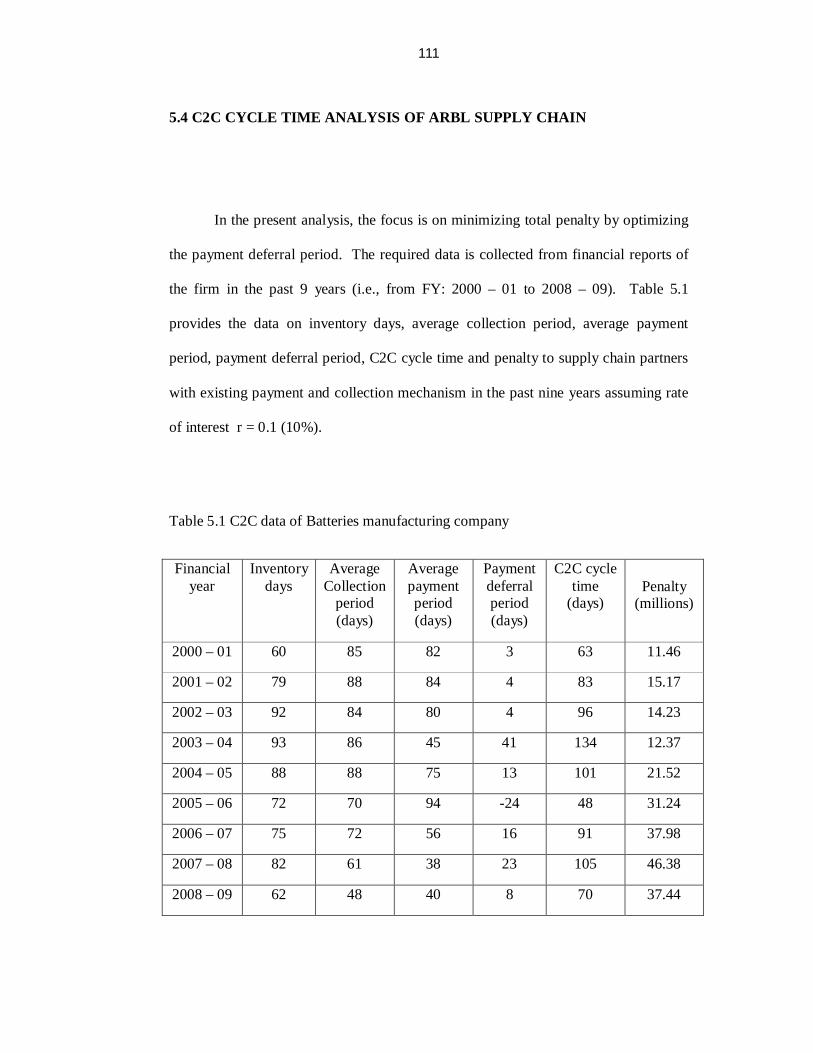
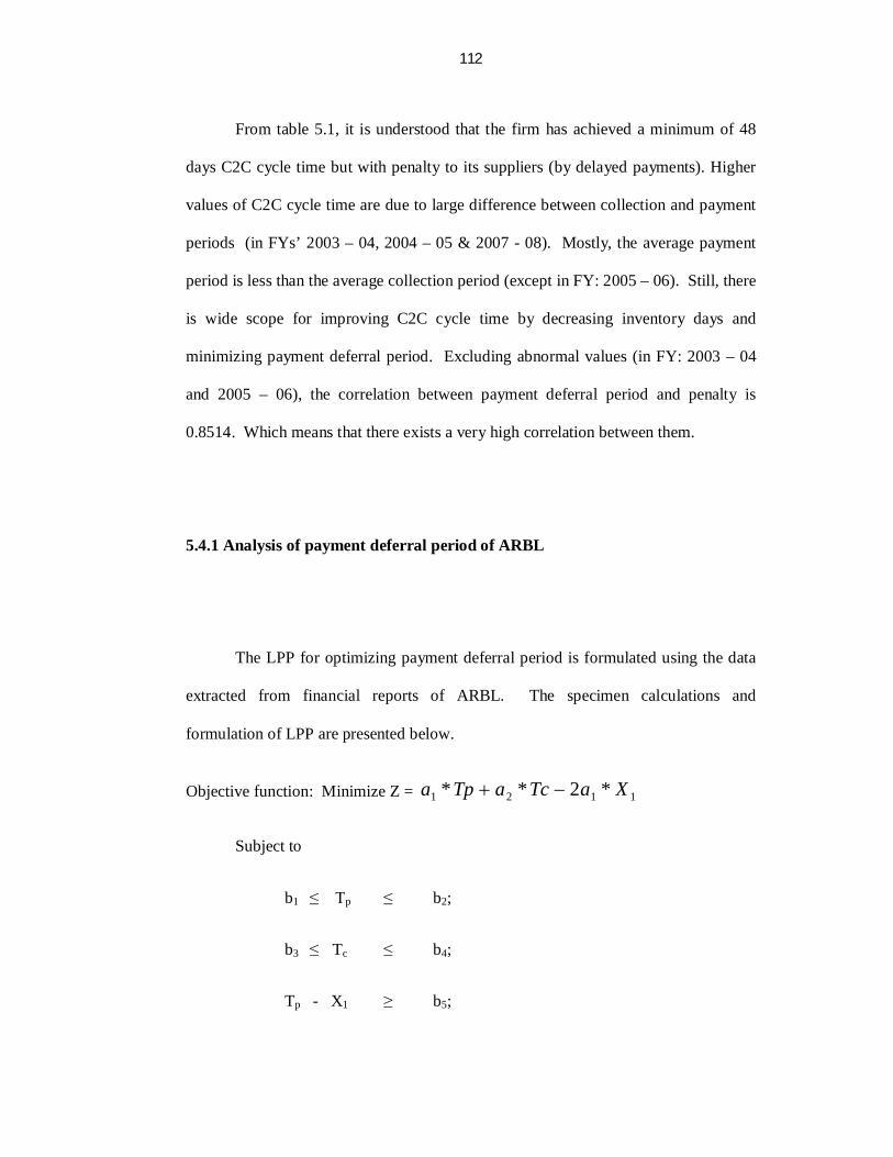
In the present analysis, the focus is on minimizing total penalty by optimizing
the payment deferral period. The required data is collected from financial reports of
the firm in the past 9 years (i.e., from FY: 2000 – 01 to 2008 – 09). Table 5.1
provides the data on inventory days, average collection period, average payment
period, payment deferral period, C2C cycle time and penalty to supply chain partners
with existing payment and collection mechanism in the past nine years assuming rate
of interest r = 0.1 (10%).
Table 5.1 C2C data of Batteries manufacturing company
Financial year
Inventory days
Average Collection
period (days)
Average payment period (days)
Payment deferral period (days)
C2C cycle time
(days) Penalty
(millions)
2000 – 01 60 85 82 3 63 11.46
2001 – 02 79 88 84 4 83 15.17
2002 – 03 92 84 80 4 96 14.23
2003 – 04 93 86 45 41 134 12.37
2004 – 05 88 88 75 13 101 21.52
2005 – 06 72 70 94 -24 48 31.24
2006 – 07 75 72 56 16 91 37.98
2007 – 08 82 61 38 23 105 46.38
2008 – 09 62 48 40 8 70 37.44
Page 8
112
From table 5.1, it is understood that the firm has achieved a minimum of 48
days C2C cycle time but with penalty to its suppliers (by delayed payments). Higher
values of C2C cycle time are due to large difference between collection and payment
periods (in FYs’ 2003 – 04, 2004 – 05 & 2007 - 08). Mostly, the average payment
period is less than the average collection period (except in FY: 2005 – 06). Still, there
is wide scope for improving C2C cycle time by decreasing inventory days and
minimizing payment deferral period. Excluding abnormal values (in FY: 2003 – 04
and 2005 – 06), the correlation between payment deferral period and penalty is
0.8514. Which means that there exists a very high correlation between them.
5.4.1 Analysis of payment deferral period of ARBL
The LPP for optimizing payment deferral period is formulated using the data
extracted from financial reports of ARBL. The specimen calculations and
formulation of LPP are presented below.
Objective function: Minimize Z = 1121 *2** XaTcaTpa
Subject to
b1 ≤ Tp ≤ b2;
b3 ≤ Tc ≤ b4;
Tp - X1 ≥ b5;
Page 9
113
Tc - X2 ≥ b6;
Tc - Tp ≥ b7;
Tp, Tc, X1, X2 ≥ 0.
The values of payables and receivables are extracted from table 3.5 and the
specimen calculations are carried out for the year 2000 – 01 as follows.
Specimen Calculation:
Payables = 133.496712 million rupees
Receivables = 361.964041 million rupees
365
*1
rPayablesa
365
1.0*496712.133
= 0.0365 ≈ 0.04
365
*Re2
rceivablesa
3651.0*964041.361
= 0.0992 ≈ 0.1
Page 10
114
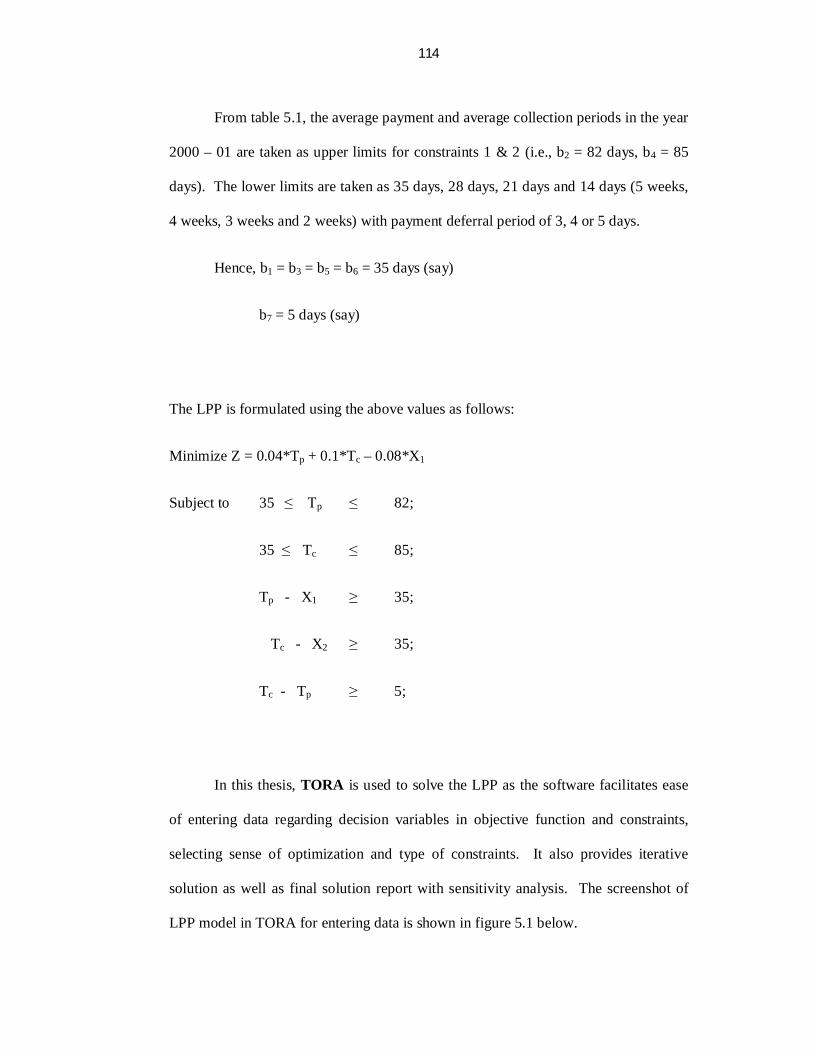
From table 5.1, the average payment and average collection periods in the year
2000 – 01 are taken as upper limits for constraints 1 & 2 (i.e., b2 = 82 days, b4 = 85
days). The lower limits are taken as 35 days, 28 days, 21 days and 14 days (5 weeks,
4 weeks, 3 weeks and 2 weeks) with payment deferral period of 3, 4 or 5 days.
Hence, b1 = b3 = b5 = b6 = 35 days (say)
b7 = 5 days (say)
The LPP is formulated using the above values as follows:
Minimize Z = 0.04*Tp + 0.1*Tc – 0.08*X1
Subject to 35 ≤ Tp ≤ 82;
35 ≤ Tc ≤ 85;
Tp - X1 ≥ 35;
Tc - X2 ≥ 35;
Tc - Tp ≥ 5;
In this thesis, TORA is used to solve the LPP as the software facilitates ease
of entering data regarding decision variables in objective function and constraints,
selecting sense of optimization and type of constraints. It also provides iterative
solution as well as final solution report with sensitivity analysis. The screenshot of
LPP model in TORA for entering data is shown in figure 5.1 below.
Page 11
115
Figure 5.1 Screen shot showing the formulation of LPP in TORA
The computations have been made for different right hand side values of
constraints and coefficients in objective function. In each case, an optimal solution is
obtained. The results clearly indicate that the optimal combination of average
payment period and average collection period are acceptable for pair(s) of trading
partners both upstream and downstream the supply chain.
Page 12
116
Table 5.2 provides the optimal average collection and payment periods for
which the total penalty will be minimum (at rate of interest r = 10%) by solving LPP
model using TORA. The analysis carried out for different Right Hand Side (RHS)
values (taking 2 weeks, 3 weeks, 4weeks and 5 weeks as payment period) reveal that
the penalty decreases with decrease in payment deferral period as well as average
payment and collection periods.
Table 5.2 Optimal payment & collection periods for ARBL (FY: 2000-01)
Payment period (14 days)
Payment period (21 days)
Payment period (28 days)
Payment period (35 days)
Optimal Tp (days)
14 14 14 21 21 21 28 28 28 35 35 35
Optimal Tc (days)
17 18 19 24 25 26 31 32 33 38 39 40
Optimal Deferral period (days)
3 4 5 3 4 5 3 4 5 3 4 5
Penalty
(Millions) 2.26 2.36 2.46 3.24 3.34 3.44 4.22 4.32 4.42 5.2 5.3 5.4
(a1 = 0.04, a2 = 0.1 for payables = 133 millions & receivables = 362 millions)
The penalty values in table 5.2 for different payment periods reveals that the
total penalty along the supply chain is decreasing as the payment and collection
period are decreased, for the given values of receivables and payables (sundry debtors
and sundry creditors). The screen shots of formulation and solution of LPP using
TORA for different values of objective function coefficients and RHS values (from
Page 13
117
FY: 2000 – 01 to 2008 – 09) are furnished in appendix – A. The optimal payment and
collection periods associated with minimum penalty in successive financial years have
been furnished in tables 5.3 to 5.10.
Table 5.3 Optimal payment & collection periods for ARBL (FY: 2001 - 02)
Payment period (14 days)
Payment period (21 days)
Payment period (28 days)
Payment period (35 days)
Optimal Tp (days) 14 14 14 21 21 21 28 28 28 35 35 35
Optimal Tc (days) 17 18 19 24 25 26 31 32 33 38 39 40
Optimal Deferral period (days)
3 4 5 3 4 5 3 4 5 3 4 5
Penalty
(Millions) 2.81 2.93 3.06 4.03 4.15 4.27 5.24 5.37 5.49 6.46 6.59 6.71
(a1 = 0.05, a2 = 0.124 for payables = 184 millions & receivables = 453 millions)
Table 5.4 Optimal payment & collection periods for ARBL (FY: 2002 - 03)
Payment period (14 days)
Payment period (21 days)
Payment period (28 days)
Payment period (35 days)
Optimal Tp (days) 14 14 14 21 21 21 28 28 28 35 35 35
Optimal Tc (days) 17 18 19 24 25 26 31 32 33 38 39 40
Optimal Deferral period (days)
3 4 5 3 4 5 3 4 5 3 4 5
Penalty
(Millions) 2.78 2.91 3.03 3.99 4.11 4.24 5.19 5.32 5.44 6.39 6.52 6.64
(a1 = 0.047, a2 = 0.125 for payables = 173 millions & receivables = 456 millions)
Page 14
118
Table 5.5 Optimal payment & collection periods for ARBL (FY: 2003 - 04)
Payment period (14 days)
Payment period (21 days)
Payment period (28 days)
Payment period (35 days)
Optimal Tp (days) 14 14 14 21 21 21 28 28 28 35 35 35
Optimal Tc (days) 17 18 19 24 25 26 31 32 33 38 39 40
Optimal Deferral period (days)
3 4 5 3 4 5 3 4 5 3 4 5
Penalty
(Millions) 2.58 2.71 2.84 3.68 3.81 3.94 4.78 4.91 5.04 5.88 6.01 6.14
(a1 = 0.0279, a2 = 0.129 for payables = 102 millions & receivables = 472 millions)
Table 5.6 Optimal payment & collection periods for ARBL (FY: 2004 - 05)
Payment period (14 days)
Payment period (21 days)
Payment period (28 days)
Payment period (35 days)
Optimal Tp (days) 14 14 14 21 21 21 28 28 28 35 35 35
Optimal Tc (days) 17 18 19 24 25 26 31 32 33 38 39 40
Optimal Deferral period (days)
3 4 5 3 4 5 3 4 5 3 4 5
Penalty
(Millions) 4.11 4.29 4.47 5.89 6.08 6.26 7.69 7.87 8.04 9.48 9.65 9.83
(a1 = 0.0775, a2 = 0.178 for payables = 283 millions & receivables = 650 millions)
Page 15
119
Table 5.7 Optimal payment & collection periods for ARBL (FY: 2005 - 06)
Payment period (14 days)
Payment period (21 days)
Payment period (28 days)
Payment period (35 days)
Optimal Tp (days) 14 14 14 21 21 21 28 28 28 35 35 35
Optimal Tc (days) 17 18 19 24 25 26 31 32 33 38 39 40
Optimal Deferral period (days)
3 4 5 3 4 5 3 4 5 3 4 5
Penalty
(Millions) 6.19 6.43 6.66 8.94 9.17 9.41 11.7 11.9 12.2 14.4 14.7 14.9
(a1 = 0.157, a2 = 0.235 for payables = 574 millions & receivables = 857 millions)
Table 5.8 Optimal payment & collection periods for ARBL (FY: 2006 - 07)
Payment period (14 days)
Payment period (21 days)
Payment period (28 days)
Payment period (35 days)
Optimal Tp (days) 14 14 14 21 21 21 28 28 28 35 35 35
Optimal Tc (days) 17 18 19 24 25 26 31 32 33 38 39 40
Optimal Deferral period (days)
3 4 5 3 4 5 3 4 5 3 4 5
Penalty
(Millions) 9.14 9.54 9.94 13.1 13.5 13.9 17.1 17.5 17.9 21.0 21.4 21.8
(a1 = 0.167, a2 = 0.4 for payables = 608 millions & receivables = 1460 millions)
Page 16
120
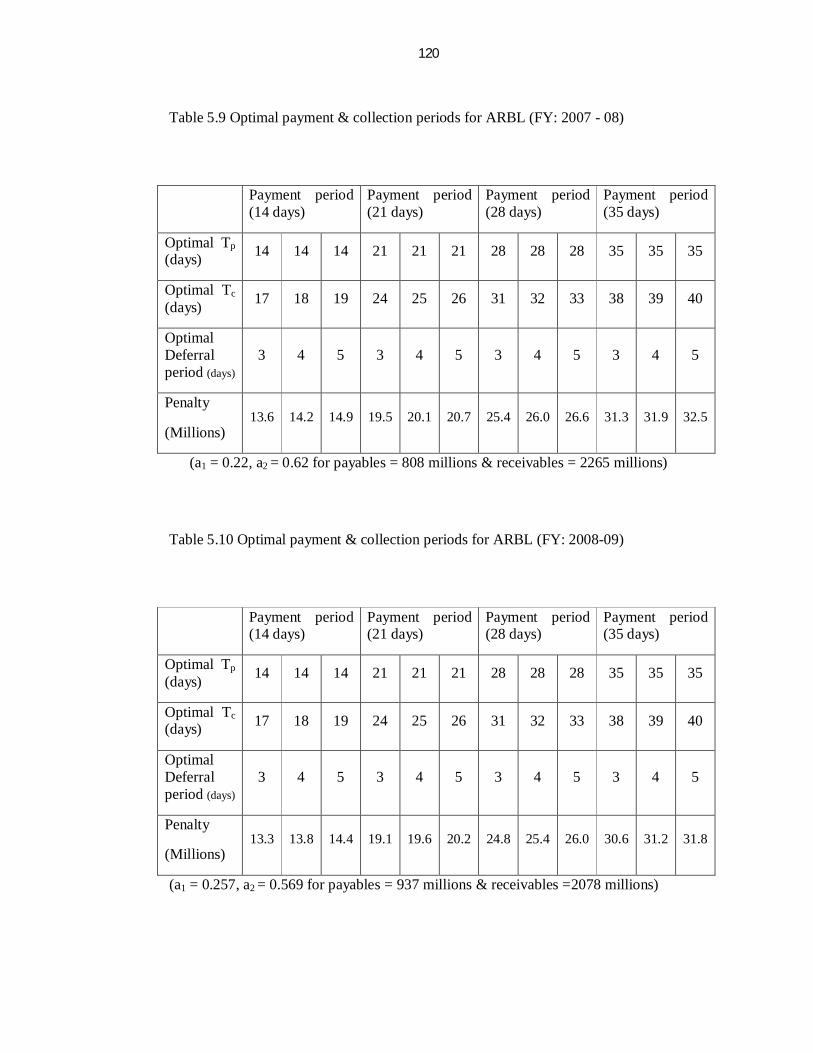
Table 5.9 Optimal payment & collection periods for ARBL (FY: 2007 - 08)
Payment period (14 days)
Payment period (21 days)
Payment period (28 days)
Payment period (35 days)
Optimal Tp (days) 14 14 14 21 21 21 28 28 28 35 35 35
Optimal Tc (days) 17 18 19 24 25 26 31 32 33 38 39 40
Optimal Deferral period (days)
3 4 5 3 4 5 3 4 5 3 4 5
Penalty
(Millions) 13.6 14.2 14.9 19.5 20.1 20.7 25.4 26.0 26.6 31.3 31.9 32.5
(a1 = 0.22, a2 = 0.62 for payables = 808 millions & receivables = 2265 millions)
Table 5.10 Optimal payment & collection periods for ARBL (FY: 2008-09)
Payment period (14 days)
Payment period (21 days)
Payment period (28 days)
Payment period (35 days)
Optimal Tp (days) 14 14 14 21 21 21 28 28 28 35 35 35
Optimal Tc (days) 17 18 19 24 25 26 31 32 33 38 39 40
Optimal Deferral period (days)
3 4 5 3 4 5 3 4 5 3 4 5
Penalty
(Millions) 13.3 13.8 14.4 19.1 19.6 20.2 24.8 25.4 26.0 30.6 31.2 31.8
(a1 = 0.257, a2 = 0.569 for payables = 937 millions & receivables =2078 millions)
Page 17
121
From tables 5.2 to 5.10, it could be understood that the penalty is decreasing
with decrease in payment and collection periods as well as the deferral period. Also,
the optimal payment and collection periods are independent of the current payment
and collection periods of the firm.
The sensitivity analysis reports for different objective coefficients and RHS
values of constraints from FY: 2000 – 01 to 2008 – 09 is furnished in appendix – B.
The results of sensitivity analyses for different objective coefficients are presented in
table 5.11.
The optimal solution given by the LPP model is helpful for firms while
negotiating on terms and conditions of supply. The firms can use these values during
benchmarking average payment and collection periods. Practically, some tolerance
may be allowed on either side of optimal value while taking strategic decisions.
Hence, this model helps to identify the penalty associated with different
combinations of average payment and collection periods associated with minimum
penalty and shorter C2C cycle time for any firm and its supply chain in an integrated
approach.. Through the practice of scientific estimation of payment and collection
periods, this ideology can be extended to successive echelons for the profit of all
firms along the supply chain.
Page 18
122
Table 5.11 Results of sensitivity analysis for different objective coefficients
Financial
year
Payables
(million
Rupees)
Receivables
(million
Rupees)
Objective Coefficients
a1 a2 X1
Current Min Max Current Min Max Current Min Max
2000 - 01 133 362 0.0400 -0.0200 α 0.1000 0.0400 α -0.0800 -0.1400 α
2001 - 02 184 453 0.0500 -0.0240 α 0.1240 0.0500 α -0.1000 -0.1740 α
2002 - 03 173 456 0.0470 -0.0310 α 0.1250 0.0470 α -0.0940 -0.1720 α
2003 - 04 102 472 0.0279 -0.0732 α 0.1290 0.0279 α -0.0558 -0.1569 α
2004 - 05 283 650 0.0775 -0.0230 α 0.1780 0.0775 α -0.1550 -0.2555 α
2005 - 06 574 857 0.1570 0.0790 α 0.2350 0.1570 α -0.3140 -0.3920 α
2006 - 07 608 1460 0.1670 -0.0660 α 0.4000 0.1670 α -0.3340 -0.5670 α
2007 - 08 808 2265 0.2200 -0.1800 α 0.6200 0.2200 α -0.4400 -0.8400 α
2008 - 09 937 2078 0.2570 -0.0550 α 0.5690 0.2570 α -0.5140 -0.8260 α
Page 19
123
5.5 INVENTORY TURNOVER RATIO
ITR is defined as the ratio of sales to average inventory with both numerator
and denominator being valued at either selling price or original cost. The success of
any firm basically depends on how efficiently it is controlling its inventories existing
in various forms at different stages of the operations of the firm. Manufacturing firms
need to maintain inventories to accommodate unexpected fluctuations in demand and
supply.
The volume of inventories depends on procurement lead time, the firm’s
purchasing strategies such as taking advantage of price discounts on bulk purchases,
geographical location of suppliers, scarcity of raw materials, expected rise in prices,
the accuracy of demand forecast, extent of subcontracting and service level of the
firm.
By formulating strategic partnership with suppliers, adapting VMI, strategic
sourcing decisions such as make / buy / sub-contracting, developing supplier relations
(shared vision and objectives), tracking of inventory (Ashwani Kumar, 2007),
minimizing inventory record keeping errors (Elgar Fleisch, Christian Tellkamp,2005),
customer relationship management (CRM) and so on, the firms can operate with
minimum levels of inventory.
Page 20
124
A significant number of inventory related issues such as inventory inaccuracy
and its impact on supply chain performance [George M Sheppard & Karen A. Brown
(1993), Elgar Fleisch & Christian Tellkamp (2005)], multi-echelon inventory
management system [A. Alfieri & R. Brandimarte (1997)], inventory capability &
distribution system flexibility [Prashant C. Palvia & D. Lim (2001)], bullwhip effect
[Richard Metters (1997), A. Gunasekaran & E.W.T. Ngai, (2004), Bradley Hull
(2005), Jiuh-Biing Sheu (2005)], expected inventory level and the stock out
probability [Ming Dong & F. Frank Chen (2005)], global inventory visibility [Scott
J.Mason et al., (2003)] and Inventory-Distribution coordination [Douglas J. Thomas
& Paul M. Griffin (1996)], impact of VMI on buyer-supplier relationship in a single
echelon supply chain [A. Mahamani & Dr. K. Prahlada Rao (2010)] have been
analyzed by researchers.
So far, there is no focus of earlier researchers on the effect of ITR on supply
chain performance. ITR is also an important aspect in inventory management which
reflects the performance of a firm and its supply chain.
C. Madhusudhana Rao & Dr. K. Prahlada Rao (2009) carried out a case study
in batteries manufacturing firm (i.e., ARBL) considering ITR as a supply chain
performance measure. The methodology to calculate ITR and analysis of ITR
discussed in this chapter is published in Serbian Journal of Management, an
International Journal for Theory and Practice of Management Science, Volume: 4
Number: 1, in the year 2009.
Page 21
125
Inventory turnover is best thought of as the number of times that an
inventory "turns over" or cycles through the firm in a year. Inventory turnover of 12
means the average inventory moves through the firm once per month. For a number of
years top-class companies have been focusing on SCM for improving their
competitiveness. They were able to demonstrate their success through improved
revenue, profit margins and decreased costs (Peter Bolstorff, 2002).
Lean is a great method to help organize work areas, reduce WIP and speedup
material flow through the entire manufacturing process. Successful lean initiatives
yield lower inventory cost, higher productivity and flexibility and faster response time
to the customer. ITR is an important measure of performance that indicates the
effective utilization of financial resources of the firm.
Inventory for customer use is an expensive investment of company money.
Instead of investing in people, technology or other important assets that can
potentially assist in growing a business faster, companies who invest in inventory
have no Return On Net Assets (RONA) until they sell the inventory.
In many businesses, inventory is turning at the lowest levels in history and
below industry averages. Studies have shown that manufacturers and wholesalers
have over 60 days of inventory and that retailers have over 90 days of inventory
Page 22
126
capital tied up. These times (inventory days) do not include inbound inventory in the
supply chain. Real supply chain inventory is 25% higher.
5.5.1 Various causes for inventory
The following are the causes for accumulation of inventory in any firm and its
supply chain.
(a) Revisions and variance in Supply Chain Management Inputs
(b) Inadequate process norms
(c) Non moving stocks
(d) High lead times & batch quantities
(e) Variance in material receipt
(f) Variance in consumption with actual versus Bill of Material
(g) Design and type changes without valid lead time.
5.5.2 The inventory turnover formula
Inventory turnover is a critical performance metric to assess the effectiveness
of inventory management. Because it is so extensively used as a diagnostic tool, it is
Page 23
127
imperative that inventory turnover be calculated using appropriate and valid
techniques.
Inventory turnover is calculated using the following formula:
ITR = monthspasttheduringinvestmentinventoryAverage
monthspasttheduringsalesstockfromSoldGoodsofCost12
12 ------- (5.9)
Alternately, the firms using Manufacturing Resource Planning (MRP - II)
software are using the following relations also to calculate ITR.
(a) ITR = 12monthcurrentofinventoryEnding
monthcurrentinsalesforsoldgoodsofCost ----------- (5.10)
(b) ITR = 12monthpreviousforinventoryEnding
monthcurrentinsalesforsoldgoodsofCost ----------- (5.11)
When product flow varies throughout the year and inventories expand and
contract during different periods, more frequent measures of the inventory level need
to be taken to generate an accurate measure of the average inventory. The inventory
turnover often is reported as the inventory period, which is the number of days’ worth
of inventory on hand, calculated by dividing the inventory by the average daily cost of
goods sold. This metric not only helps a firm as diagnostic measure but also helps to
improve C2C cycle time of a firm.
Page 24
128
Inventory Period (days) = 365cos
soldgoodsoftAnnual
inventoryAverage ------ (5.12)
The following points kept in mind when calculating turnover ratio:
1. Consider only cost of goods sold from stock sales which are filled from
warehouse inventory. Non-stock items and direct shipments are not included.
2. The cost of goods sold figure in the formula includes transfers of stocked
products to other branches and quantities of these products used for internal
purposes such as repairs and assemblies.
3. Inventory turnover is based on the cost of items (what the company paid for
them) but not sales dollars (what the company sold them for).
Inventory turnover depends on the average value of stocked inventory. To
determine average inventory investment,
1. The total value of every product in inventory is to be calculated (quantity on-
hand times cost) every month, on the same day of the month. One must be
consistent in using the same cost basis (average cost, last cost, replacement
cost, etc.) in calculating both the cost of goods sold and average inventory
investment.
Page 25
129
2. If the company’s inventory levels tend to fluctuate throughout the month, then
it has to calculate the total inventory value on the first and fifteenth of every
month.
3. To determine the average inventory value, a firm has to take average of all
inventory valuations recorded during the past 12 months.
All the above points were considered while collecting data and manipulated as
per the requirements of the present research work.
5.5.3 Turnover goals
1. As a company determines its inventory turnover goals, it should consider the
average gross margin it receives on the sale of products. Most distributors who
have 20% - 30% gross margins should strive to achieve an overall turnover rate of
five to six turns per year. Distributors with lower margins require higher stock
turnover. If the company enjoys high gross margins, it can afford to turn its
inventory less often.
Page 26
130
2. A turnover rate of six turns per year doesn’t mean that the stock of every item will
turn six times. The stock of popular, fast moving items should turn more often (up
to 12 times per year). Slow moving items may turn only once, or not at all.
3. Finally, inventory turnover should be calculated separately for every product line
in every warehouse. This will allow a company to identify situations in which its
inventory is not providing an adequate return on investment. To improve
inventory turnover, a company should consider reducing the quantity it normally
buy from the supplier. Inventory turns improve when a company buys less of
product, more often.
4. Companies have limited funds available to invest in inventory. They cannot
stock a lifetime supply of every item. In order to generate the cash necessary to
pay their bills and return a profit, one must sell the materials they have bought.
The inventory turnover rate measures how quickly the firm is moving inventory
through its warehouse. Combined with other measurements such as customer
service level and return on investment, inventory turnover can provide an accurate
barometer of a company’s success.
Page 27
131
5.6 ANALYSIS OF INVENTORY TURNOVER RATIO
As this performance metric reflects not only the internal operational
performance but also affects the working capital management of a firm, this is more
important performance measure. The companies can benchmark ITR by computing
current ITR value and comparing with that of the companies in the same industry
sector. If benchmark values are not available, a firm can set benchmark levels by
itself basing on earlier performance. As the inventory days depends on ITR, larger
the value of ITR, smaller will be the inventory days and in turn shorter the C2C cycle
time.
5.6.1. ITR calculations of IBD
In the present research work, the ITR of IBD has been analyzed. After finding
the gaps in performance (in terms of ITR), a set of alternatives have been identified to
increase ITR. The courses of action adapted for implementation are furnished below:
(a) Revision of stocking policy of A - class materials so as to maintain stocks for
15 to 20 days of consumption.
(b) Revision of ordering policy for B & C - class items as per lead time and
Economic Order Quantity (EOQ) of purchase department.
Page 28
132
(c) MRP computation as per 1 + 2 months production plan.
(d) To reduce the forecast variance of marketing (Market Research Information).
(e) Information on design and type changes with valid lead time and clear action
to dilute existing stocks.
Implementation of these plans has improved the ITR of industrial battery
division tremendously in the past five years. The data required to calculate ITR is
obtained from sales data and inventory levels of raw materials, work in process and
finished goods including those in transit and available at ware houses / market outlets.
As a part of continuous improvement program, by closely monitoring the ITR, a firm
can continuously improve its capability to rotate money as many times as possible in a
year. Specimen calculation of ITR and inventory days for the month May – 2004 is
given below. The ITR trend of IBD in the past five financial years calculated using
equation (5.11) is furnished in the tables 5.12 to 5.16.
Specimen Calculation:
The Net Sales in the month May – 2004 = 125 Million Rupees
Ending inventory of the month April – 2004 = 309.6 Million Rupees
Inventory Turnover Ratio (ITR) in May - 2004 = 126.309
125
= 4.8
Page 29
133
Inventory Days for the month May – 2004 = ITR365 Days
= 8.4
365
= 75.35 days
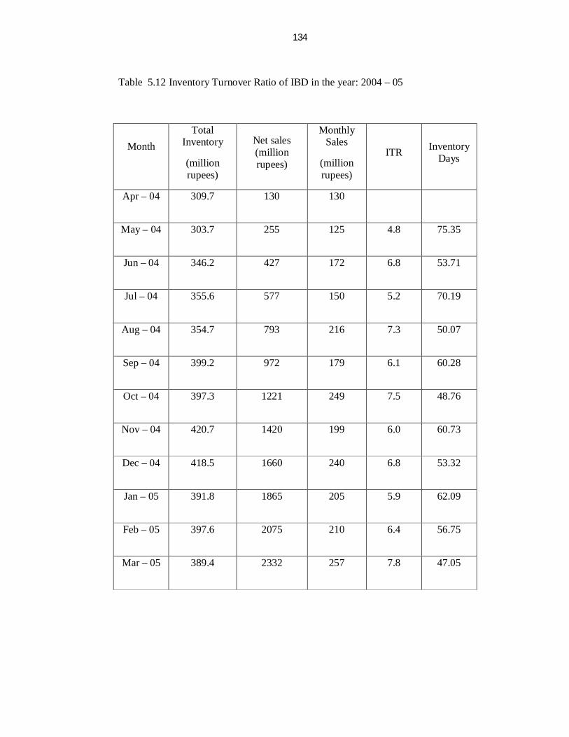
Similarly, the ITR and Inventory Days of Supply (IDS) have been calculated
for each month from May – 2004 to March – 2009. The values furnished in tables:
5.11 to 5.15 indicate improved ITR with corresponding decrease in IDS (calculated
using equation 5.12) during that period.
Page 30
134
Table 5.12 Inventory Turnover Ratio of IBD in the year: 2004 – 05
Month Total
Inventory
(million rupees)
Net sales (million rupees)
Monthly Sales
(million rupees)
ITR Inventory Days
Apr – 04 309.7 130 130
May – 04 303.7 255 125 4.8 75.35
Jun – 04 346.2 427 172 6.8 53.71
Jul – 04 355.6 577 150 5.2 70.19
Aug – 04 354.7 793 216 7.3 50.07
Sep – 04 399.2 972 179 6.1 60.28
Oct – 04 397.3 1221 249 7.5 48.76
Nov – 04 420.7 1420 199 6.0 60.73
Dec – 04 418.5 1660 240 6.8 53.32
Jan – 05 391.8 1865 205 5.9 62.09
Feb – 05 397.6 2075 210 6.4 56.75
Mar – 05 389.4 2332 257 7.8 47.05
Page 31
135
Table 5.13 Inventory Turnover Ratio of IBD in the year: 2005 – 06
Month Total
Inventory
(million rupees)
Net sales (million rupees)
Monthly Sales
(million rupees)
ITR Inventory Days
Apr – 05 399.2 210 210 6.5 56.40
May – 05 386.9 459 249 7.5 48.71
Jun – 05 412.5 726 267 8.3 44.08
Jul – 05 429.8 961 235 6.8 53.39
Aug – 05 431.2 1255 294 8.2 44.51
Sep – 05 481.0 1534 279 7.8 47.06
Oct – 05 482.4 1863 329 8.2 44.43
Nov – 05 467.4 2212 349 8.7 42.04
Dec – 05 435.2 2567 355 9.1 40.06
Jan – 06 456.6 2950 383 10.6 34.53
Feb – 06 435.6 3309 359 9.4 38.73
Mar – 06 404.6 3701 392 10.8 33.80
Page 32
136
Table 5.14 Inventory Turnover Ratio of IBD in the year: 2006 – 07
Month Total
Inventory
(million rupees)
Net sales (million rupees)
Monthly Sales
(million rupees)
ITR Inventory Days
Apr – 06 449.0 389 389 11.5 34.43
May – 06 492.3 792 403 10.8 33.89
Jun – 06 519.5 1231 439 10.7 34.11
Jul – 06 560.1 1703 472 10.9 33.48
Aug – 06 654.9 2198 495 10.6 34.42
Sep – 06 690.9 2782 584 10.7 34.11
Oct – 06 727.0 3398 616 10.7 34.11
Nov – 06 655.0 4077 679 11.2 32.57
Dec – 06 626.6 4693 616 11.3 32.34
Jan – 07 605.3 5298 605 11.6 31.50
Feb – 07 557.8 5863 565 11.2 32.59
Mar – 07 471.7 6407 544 11.7 31.19
Page 33
137
Table 5.15 Inventory Turnover Ratio of IBD in the year: 2007 – 08
Month Total
Inventory
(million rupees)
Net sales (million rupees)
Monthly Sales
(million rupees)
ITR Inventory Days
Apr – 07 667.1 528 528 13.4 27.13
May – 07 735.0 1306 778 14.0 26.08
Jun – 07 737.3 2254 948 15.5 23.58
Jul – 07 772.3 3129 875 14.2 25.63
Aug – 07 732.4 4094 965 15.0 24.34
Sep – 07 746.3 4921 827 13.6 26.94
Oct – 07 861.0 5836 915 14.7 24.81
Nov – 07 774.4 6909 1073 15.0 24.41
Dec – 07 798.8 7854 945 14.6 24.92
Jan – 08 983.4 8801 947 14.2 25.66
Feb – 08 853.6 10165 1364 16.6 21.93
Mar – 08 788.6 11247 1082 15.2 24.00
Page 34
138
Table 5.16 Inventory Turnover Ratio of IBD in the year: 2008 – 09
Month Total
Inventory
(million rupees)
Net sales (million rupees)
Monthly Sales
(million rupees)
ITR Inventory Days
Apr – 08 1027.5 1023 1023 15.6 23.40
May – 08 973.9 2148 1125 13.1 27.78
Jun – 08 946.6 3306 1158 14.3 25.58
Jul – 08 914.8 4438 1132 14.3 25.44
Aug – 08 954.4 5621 1183 15.5 23.52
Sep – 08 875.8 6865 1244 15.6 23.34
Oct – 08 941.5 7939 1074 14.7 24.80
Nov – 08 1110.7 9152 1213 15.5 23.61
Dec – 08 1199.4 10585 1433 15.5 23.57
Jan – 09 1148.9 12128 1543 15.4 23.64
Feb – 09 1112.5 13597 1469 15.3 23.79
Mar – 09 1041.5 14934 1337 14.4 25.31
Page 35
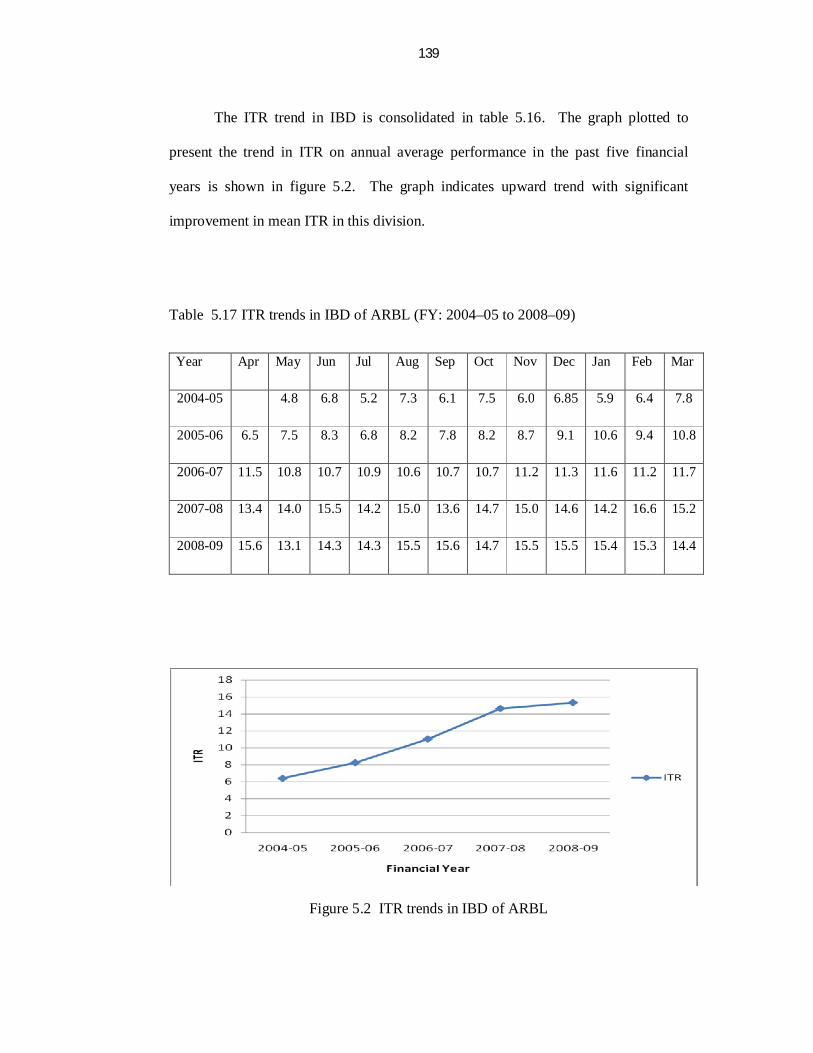
139
The ITR trend in IBD is consolidated in table 5.16. The graph plotted to
present the trend in ITR on annual average performance in the past five financial
years is shown in figure 5.2. The graph indicates upward trend with significant
improvement in mean ITR in this division.
Table 5.17 ITR trends in IBD of ARBL (FY: 2004–05 to 2008–09)
Year Apr May Jun Jul Aug Sep Oct Nov Dec Jan Feb Mar
2004-05 4.8 6.8 5.2 7.3 6.1 7.5 6.0 6.85 5.9 6.4 7.8
2005-06 6.5 7.5 8.3 6.8 8.2 7.8 8.2 8.7 9.1 10.6 9.4 10.8
2006-07 11.5 10.8 10.7 10.9 10.6 10.7 10.7 11.2 11.3 11.6 11.2 11.7
2007-08 13.4 14.0 15.5 14.2 15.0 13.6 14.7 15.0 14.6 14.2 16.6 15.2
2008-09 15.6 13.1 14.3 14.3 15.5 15.6 14.7 15.5 15.5 15.4 15.3 14.4
Figure 5.2 ITR trends in IBD of ARBL
Page 36
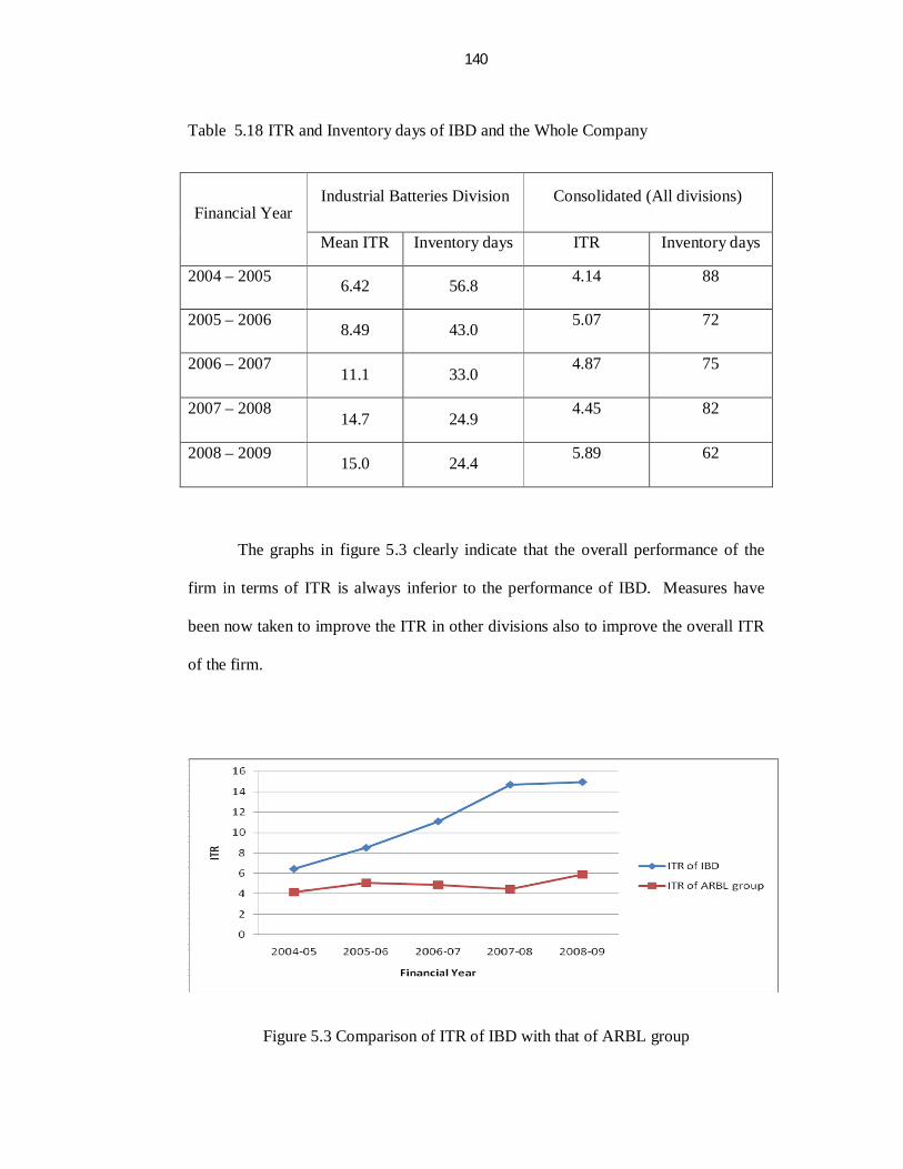
140
Table 5.18 ITR and Inventory days of IBD and the Whole Company
Financial Year Industrial Batteries Division Consolidated (All divisions)
Mean ITR Inventory days ITR Inventory days
2004 – 2005 6.42 56.8 4.14 88
2005 – 2006 8.49 43.0 5.07 72
2006 – 2007 11.1 33.0
4.87 75
2007 – 2008 14.7 24.9
4.45 82
2008 – 2009 15.0 24.4 5.89 62
The graphs in figure 5.3 clearly indicate that the overall performance of the
firm in terms of ITR is always inferior to the performance of IBD. Measures have
been now taken to improve the ITR in other divisions also to improve the overall ITR
of the firm.
Figure 5.3 Comparison of ITR of IBD with that of ARBL group
Page 37
141
The results of analysis indicate clearly that the benefit of improving ITR or
decreasing inventory days is two fold: Firstly, the working capital management will
be more effective. Secondly, the C2C cycle time will be improved which leads to
lesser penalty to all parties along the supply chain and better buyer-supplier
relationships along the value chain.
5.7 SUMMARY
In this chapter, the attempt is to develop LPP model to find optimal payment
and collection periods that would minimize penalty to all the entities i.e., suppliers,
firm and customers. The data collected from financial reports of ARBL is analyzed
and optimal payment and collection periods associated with minimal penalty have
been found in each case. The results of analysis strongly support that the penalty will
be less when payment period and diferral periods are short which in turn will lead to
shorter C2C cycle time. Also, this analysis helps firms in benchmarking payment and
collection periods at supplier and customer ends for the benefit of all the firms along
the supply chain in an integrated approach. The analysis of ITR also strongly support
that improved ITR will help firms in optimizing their inventory management and at
the same time, the small the inventory days shorter will be the C2C cycle time.
Hence, it is essential for firms in an integrated supply chain management to focus on
improved ITR through inventory visibility and collaborative planning forecasting and
replenishment that helps all the firms along the supply chain.