To: Dr. Colin McCullough Specialty Materials Division Composite Conductor Program 3M Company 3130 Lexington Ave So Eagan, MN 55121 USA KINECTRICS NORTH AMERICA INC. TEST REPORT FOR 3M COMPANY TO DETERMINE THE SAG – TEMPERATURE – TENSION PERFORMANCE OF 675TW 3M BRAND COMPOSITE CONDUCTOR Kinectrics North America Inc. Report No.: K-422008-RC-0001-R01 June 23, 2005 C.J. Pon Transmission and Distribution Technologies Business INTRODUCTION A Sag – Temperature – Tension Test was performed for 3M Company on their 3M Brand Composite Conductor, which is also known as Aluminium Conductor Composite Reinforced (ACCR) Conductor. This test is part of a larger series of tests to demonstrate the viability of ACCR conductors for use on overhead electric power transmission lines. The tests were performed by Kinectrics North America Inc. personnel at 800 Kipling Avenue, Toronto, Ontario, M8Z 6C4, Canada. . 3M Company owns all data and copyright to this information and are publicly released by 3M. A sag-tension-temperature study on 675TW showed a knee-point transition in the range of 80- 100°C. The “compressive stress parameter” or “built-in tensile stress parameter” should be set at –1.45 ksi (-10MPa) for the line design software programs. The line design software programs such as Alcoa Sag10 and STESS predict the sag-tension-temperature behaviour very well. Kinectrics North America Inc., 800 Kipling Avenue, Toronto, Ontario M8Z 6C4.
Transcript
To: Dr. Colin McCullough Specialty Materials Division Composite Conductor Program 3M Company 3130 Lexington Ave So Eagan, MN 55121
USA
KINECTRICS NORTH AMERICA INC. TEST REPORT FOR 3M COMPANY TO DETERMINE THE SAG – TEMPERATURE – TENSION
PERFORMANCE OF 675TW 3M BRAND COMPOSITE CONDUCTOR
Kinectrics North America Inc. Report No.: K-422008-RC-0001-R01 June 23, 2005
C.J. Pon
Transmission and Distribution Technologies Business INTRODUCTION A Sag – Temperature – Tension Test was performed for 3M Company on their 3M Brand Composite Conductor, which is also known as Aluminium Conductor Composite Reinforced (ACCR) Conductor. This test is part of a larger series of tests to demonstrate the viability of ACCR conductors for use on overhead electric power transmission lines. The tests were performed by Kinectrics North America Inc. personnel at 800 Kipling Avenue, Toronto, Ontario, M8Z 6C4, Canada. . 3M Company owns all data and copyright to this information and are publicly released by 3M. A sag-tension-temperature study on 675TW showed a knee-point transition in the range of 80-100°C. The “compressive stress parameter” or “built-in tensile stress parameter” should be set at –1.45 ksi (-10MPa) for the line design software programs. The line design software programs such as Alcoa Sag10 and STESS predict the sag-tension-temperature behaviour very well.
Kinectrics North America Inc., 800 Kipling Avenue, Toronto, Ontario M8Z 6C4.
TEST OBJECTIVE The objective of the Sag – Temperature – Tension Test was to determine the sag and tension of the 675TW kcmil ACCR conductor when subjected to increasing temperatures. The composite core of 3M’s ACCR conductors has a lower coefficient of thermal expansion and higher conductivity than the steel core in conventional ACSR conductors. The Sag – Temperature – Tension Test tests would provide information on whether these differences affect the thermal and physical response of the ACCR conductors. TEST CONDUCTOR The conductor tested was designated ACCR/675TW, 20/7 manufactured by 3M Company. The construction of this conductor has 20 aluminum alloy wires in 2 layers surrounding seven core wires. The outside diameter of the conductor is 22.91mm (0.902 inches). The data sheet on the 675TW kcmil ACCR conductor used in the sag – temperature – tension test is contained in Appendix A. Sixty-eight (68) meters of the conductor was prepared. The conductor was terminated as shown in Figure 1. Each end of the conductor was passed through aluminum housings. The conductor strands were splayed apart within a cone-shaped cavity inside the aluminum housing. High-temperature epoxy resin was poured into the cavity to “lock” all strands of the conductor together. The strands were reformed outboard of the aluminum housing and a compression terminal was compressed on the end of the conductor to allow current to be passed through the sample.
Figure 1 Epoxy dead-end
K-422008-RC-0001-R01
2
TEST SET-UP Test Apparatus The Sag – Temperature – Tension Test was carried out at Kinectrics’ Conductor Dynamics Laboratory. The laboratory is temperature controlled to 22ºC ±2ºC with minimal air movement. A schematic of the setup is shown in Figure 2. The maximum span length (ie. tension eye to tension eye) was 68.8 m. The actual conductor length was shorter than this to accommodate end hardware such as the tensioning dead-ends, insulators, load cells and other links. The sample was tensioned horizontally about 2.44m (8 feet) above the ground.
A-A Overall span length (68.8 m) G North Load Cell B-B Span length between North and South Sag Measurement H North Insulator (4 skirt) C-C Sag at mid-span J North epoxy dead-end assembly D-D Sag at North end just inboard of hardware K South Load Cell E-E Sag at South end just inboard of hardware L South Insulator (6 skirt) F Strain Plate M South epoxy dead-end assembly
Figure 2 Schematic of Test Setup A current transformer provided the circulating current to heat the cable. One end of the conductor was connected to a tap of the current transformer. The opposite end of the conductor was connected to a 795 kcmil ACSR conductor, (return conductor) to complete the circuit back to the current transformer. The 795 kcmil ACSR conductor was tensioned at the same level and 1m away from the test conductor. The test conductor and the return conductor are shown in Figure 4. Instrumentation
Conductor Tension A strain gauge load cell measured the tension in each conductor during the test. The load cell was installed between the insulator and the dead-end structure so that it would be electrically isolated from the conductor. The signal from the load cells were amplified by optically isolated signal conditioners to provide a 0 to 5 volt signal for the data acquisition system.
K-422008-RC-0001-R01
3
Conductor Temperature The temperature of the conductor was measured at two(2) locations using thermocouples. One location was at the centre of the span the other location was at halfway between the centre and one dead-end (¼ point). The core, middle aluminum layer, and outer aluminum layer were measured at each location. The following summarizes the thermocouple positions at each location. Thermocouple #1 – Next to the core Thermocouple #2 – Between two aluminum-alloy wires in the middle layer Thermocouple #3 – Between two aluminum-alloy wires in the outer layer The thermocouples were optically isolated from other instrumentation to prevent electrical interference into the data acquisition system. A typical thermocouple installation is shown in Figure 3.
Figure 3 Typical Thermocouple Installation Conductor Sag The ends of the conductor were not fixed in space during the heating and cooling because the conductor end fittings were part of the tensioned span. It was therefore necessary to measure the vertical and longitudinal position at both ends of the conductor as well the vertical position at midspan. Pull wire potentiometers were used to make these measurements for each conductor. For the vertical measurements, the potentiometer housings were mounted on fixed supports above the conductors. The pull wire was attached to the conductor and would extend from the housing as the sag increased when the conductor was heated and would retract into the housing as the sag decreased when the conductor cooled. Three (3) potentiometers were located at three (3) positions along the conductor, one at midspan and one at each end of the span.
K-422008-RC-0001-R01
4
For the longitudinal measurements, the potentiometers were mounted on fixed supports located outboard of the end fitting attachment points. The pull wire was attached to the conductor and would extend from the housing as the sag decreased when the conductor was cooled and would retract into the housing as the sag increased when the conductor was heated. Two (2) potentiometers were located at each end of the span. This setup is shown in Figure 4.
Figure 4 Test Setup Near Dead-end Data Acquisition and Control A Labview-based data logging system recorded all temperatures, sag or clearance and tension data. The system sampled every 2 seconds and saved data at a user-selected interval. The data was saved every 5 seconds when the change in sag-temperature was greater, and slowed to every 30 seconds when the conductors were at steady-state temperature. The data acquisition system also provided a 5-volt logic control signal that controlled a Silicon Controlled Rectifier (SCR) through an optically isolated output module. The data acquisition system would turn current on or off based on the thermocouple readings. Conductor temperature was considered to be the independent variable. TEST PROCEDURE The current transformers were turned “ON” and left “ON” until the test conductor reached the target temperature of 240°C. The whole conductor was considered to have reached this temperature as soon as the highest reading thermocouple measured 240°C. The current was then turned “OFF” and the conductors were allowed to cool by natural convection to room
K-422008-RC-0001-R01
5
temperature. Two (2) cycles were performed using this procedure. The details of the two cycles are listed in Table 1.
Table 1 Summary of Test Parameters
Parameter First cycle Second Cycle Max Temp. of ACCR/675TW 240ºC 239ºC Temperature rise from ambient (23ºC) 217ºC 216ºC Temp. rise time 23 minutes 43 minutes Average heating rate 9.5ºC/min 5.1ºC/min Cooling time 240ºC to 30ºC 1 hour 10 minutes 1 hour 12 minutes Average cooling rate 240ºC to 30ºC 3.0º/min 2.9º/min Cooling time 240º to ambient (23ºC) n/a 3 hours 41 minutes Average cooling rate 240ºC to ambient (23ºC) n/a 1.0º/min
TEST RESULTS A plot showing sag and tension versus conductor temperature of the conductor for Cycle 1 and 2 are shown in Figures 5 and 6 respectively. Table 2 contains a summary of the results. The conductor temperature is taken to be the highest reading thermocouple in each conductor. The temperatures of the core and aluminum layers at the start, nominally 240ºC and the end of the test are listed in Table 3. The following general observations are made about the plots. - The heating cycle produces higher sag than the cooling cycle for the same temperature.
That is, there is some hysteresis. - The test conductor does not exhibit a well-defined kneepoint temperature. The kneepoint is
a transition between 80ºC to 100ºC. - For the second cycle, after cooling back to room temperature the conductor had less sag by
15mm and higher tension 112 kg than at the start of the test.
Table 2 Summary of High Temperature Test Results
Cycle 1 23ºC
(Before Heating)
240ºC Net Change
Sag 273mm 1334mm 1061mm
Tension 2083 kg 443 kg 1640 kg
Tension (%RBS) 20.4% 4.3% 15.8%
K-422008-RC-0001-R01
6
Cycle 2 23ºC
(Before Heating)
240ºC Net Change
Sag 280mm (11.0 inches)
1382mm (54.4 inches)
1102mm (43.4inches)
Tension 2050 kg (4519 lb)
427 kg (941 lb)
1623 kg (3578 lb)
Tension (%RBS) 20.1% 4.2% 15.9%
Table 3 Temperatures of Core and Aluminum Layers
¼ Point of Span Centre of Span Cycle Core Middle Al. Outer Al. Core Middle Al. Outer Al.
1 start 23.0 22.6 22.8 22.0 22.7 22.71 240ºC 231.6 231.5 232.1 231.3 231.6 240.41 end 29.4 29.2 29.2 30.2 31.2 31.42 start 23.0 22.7 23.0 21.9 22.6 22.62 240ºC 222.6 222.6 223.1 231.1 231.2 239.42 end 23.0 22.7 22.8 22.1 22.8 22.8 Analysis Data was analyzed by Dr. Stephen Barrett of Barrett Research to look at how the data compares to predictions from transmission line design software such as Sag10 and STESS (Strain Summation method). Both calculate sag using the Alcoa graphical method. These analyses are shown in Appendix B and were performed independently of Kinectrics Inc. The “compressive stress parameter” or “built-in tensile stress parameter” should be set at –1.45 ksi (-10MPa) for the line design software programs. CONCLUSION
1. A sag-tension-temperature study on 675TW showed a knee-point transition in the range of 80-100°C.
2. The “compressive stress parameter” or “built-in tensile stress parameter” should be set at –1.45 ksi (-10MPa) for the line design software programs.
3. The line design software programs such as Alcoa Sag10 and STESS predict the sag-tension-temperature behaviour very well.
K-422008-RC-0001-R01
7
_________________________________
Prepared by: __________________________________________________ C.J. Pon Principal Engineer Transmission and Distribution Technologies Business
Approved by: _____ _____________ Dr. J. Kuffel General Manager
Transmission and Distribution Technologies Business CJP:JC
ACNOWLEDGEMENTS AND DISCLAIMER Kinectrics North America Inc. has prepared this report in accordance with, and subject to, the terms and conditions of the contract between Kinectrics North America Inc. and 3M Company, dated August 15, 2002. This material is based upon work supported by the U.S. Department of Energy under Award No. DE-FC02-02CH11111. Any opinions, findings, and conclusions or recommendations expressed in this material are those of the author(s) and do not necessarily reflect the views of the Department of Energy.
Kinectrics North America Inc., 2005.
K-422008-RC-0001-R01
8
ACCR Sag and Tension vs Temperature
0
200
400
600
800
1000
1200
1400
20 40 60 80 100 120 140 160 180 200 220 240 260Cable Temperature - deg C
Con
duct
or S
ag -
mm
0
400
800
1200
1600
2000
2400
2800
Con
duct
or T
ensi
on -
kg
Conductor Sag
Conductor Tension
Cooling
Heating
Heating
Cooling
9 K-422008-R
C-0001-R
01 Figure 5 Cycle 1 Conductor Sag and Tension vs. Temperature
ACCR Sag and Tension vs Temperature
0
200
400
600
800
1000
1200
1400
20 40 60 80 100 120 140 160 180 200 220 240 260
Cable Temperature - deg C
Con
duct
or S
ag -
mm
0
400
800
1200
1600
2000
2400
2800
Con
duct
or T
ensi
on -
kg
Conductor Sag
Conductor Tension
Cooling
Heating
Heating
Cooling
Figure 6 Cycle 2 Conductor Sag and Tension vs. Temperature
Conductor Electrical PropertiesResistance DC @ 20C ohms/mile 0.1317 AC @ 25C ohms/mile 0.1348 AC @ 50C ohms/mile 0.1481 AC @ 75C ohms/mile 0.1615
Geometric Mean Radius ft 0.0355Reactance (1 ft Spacing, 60hz) Inductive Xa ohms/mile 0.4052 Capacitive X'a ohms/mile 0.0973
K-422008-RC-0001-R01
A-2
APPENDIX B
Report on 675 kcmil (20/7) ACCR/TW
Heat-Run Tests at Kinectrics
November 24, 2003
Prepared by: Stephen Barrett, Barrett Research Barrett Research, 93 Thomas Blvd. SS3 Elora, Ont. Canada NOB 1S0 [email protected]
K-422008-RC-0001-R01
B-1
Sections
1) Introduction 2) Change of “Inner Span” with Tension. 3) Measured and Calculated Sags of ACCR 4) Measured and Calculated Sags of ACSR 5) Discussion of Compressive Stress. 6) Sag Comparison for a 1000 ft Span
1) Introduction The two heat cycles on 675 kcmil (20/7) ACCR/TW were performed by Kinectrics on October 9 & 10, 2003. The “Total Span” was approximately 225 ft. and the “Inner Span” (excluding end hardware) was 215 ft. The Hardware at the South end was 5.17 ft. long and weighed 16.4 lb. The hardware at the North end was 5.17 ft long and weighed 9.6 lb. Heat runs were performed simultaneously on a parallel sample of 795 kcmil (26/7) ACSR. Each inner-Span Sag was measured by 3 String Potentiometers (“String-Pots”), one at centre-span and one at each end of the inner span. Tension was measured by a load cell at the north end. 2) Change of Inner Span with Tension Horizontal string-pots were used to record the change of the inner span, which changed for two reasons: elastic movement of the supports and the effect of the length and weight of the terminal hardware.
Each curve can be decomposed into elastic support movement and the effect of terminal length and weight. The span gets longer as the temperature rises and the tension drops, as expected. However, there is some hysteresis in the horizontal string-pot readings and also in the sags. When the temperature drops and the tension increases, the span does not shorten all the way back to its original position. This hysteresis in span length results in a sag hysteresis, so that the sags during the decreasing-temperature portion of the heat-cycle are reduced. During the first heat cycle, the ACSR curves for rising and falling temperature are quite different, suggesting that the rising and falling curves for sag should also be different. This is not the case, however, indicating that something went wrong with the ACSR’s horizontal string-pots during part of the first cycle. This problem did not occur during the second cycle. The data suggest that the end supports are not twisting very much. (Both spans elongate elastically at approximately the same rate as a function of the tension of each conductor individually). It is not clear whether the support movements for the two conductors are independent or whether the two conductors cooperate in moving the supports. From the point of view of data analysis, it doesn't really matter.
K-422008-RC-0001-R01
B-3
The span-elongation curves were fitted by:
δS/S = C – ELAST x H + TERM / H2 for tension H in kN.
ELAST TERM ACCR 8 x 10⁻⁶ .005 ACSR 8 x 10⁻⁶ .008
The constant term defines a reference span length and may be discarded after fitting. Discarding this term defines the reference inner span length as the length of the span without conductor (zero tension on the supports) and with the terminal hardware held in a horizontal orientation. The linear term is elastic movement of the supports. The 1/H2 term accounts for the effect of the length and weight of the terminal hardware. This fit is entered into the sag-tension program in order to take the changing span length into account when calculating sags and tensions. The theoretical value of “TERM” is given by: ])()([)8/1( 22
RRLL MwSLMwSLSTERM +++= where S = 215 ft w = 0.726 lb/ft The terminal lengths are each 5.17 ft The terminal weights are 16.4 lb (south) and 9.6 lb (north) These values lead to a theoretical value of TERM = 172 lb2 = 0.0034 kN2 for the ACCR. The measured value was 0.005, which is somewhat higher. This may be because it is difficult to completely eliminate the weight of the current connections and leads during the test. This weight was not taken into account in the theoretical calculation. The measured value was used to correct the sag-tension calculations.
The sags as measured by string-pots are in very close agreement with those computed from the load-cell tensions. Sags were also calculated by the Strain-Summation Method for zero compressive aluminum stress and for –1.45 ksi above the knee-point temperature. The knee-point is not very distinct in this case and is smeared between 70°C and 90°C. The high-temperature sags fall between the 0 ksi and –1.45 ksi curves, except for some string-pot measurements during the second heat cycle, which slightly exceed the –1.45 ksi curve. (The corresponding Load-Cell sags coincide with the –1.45 ksi curve. The continued use of –1.45 ksi (-10 MPa) compressive aluminum stress is recommended. The hysteresis that was seen in the change of span length in the first graph, shows up as reduced sags during the decreasing-temperature portion of the heat cycle. A small proportion of this hysteresis may also be cause by hysteresis in the stress-strain curves, which is not normally considered in sag-tension programs. The small increase of sag (~50 mm) in cycle 2 compared with cycle 1 is likely due a slight twisting of the supports because there is the same amount of discrepancy in the ACSR data below, but in the opposite direction. The data have not been corrected for support movement but the fits have been corrected in an attempt to match the observed sags. The support movement was fitted to cycle 1 and the same parameters were used for cycle 2. Perhaps a more careful fitting of the support movement in cycle 2 would correct these small discrepancies.
K-422008-RC-0001-R01
B-5
4) Measured and Calculated Sags of ACSR
Sag of 795 kcmil (26/7) ACSR "Drake" - 215 ft. Span
5) Discussion of Compressive Stress Over the past few decades, it has become normal practice (STESS) to use a default value of compressive aluminum stress (-10 MPa or -1.45 ksi) at high temperatures. As can be seen in the ACCR graph, above, this would add approximately 165 mm (6.5 inches) to the calculated sag. This precaution would overestimate the calculated sag at 240°C by approximately 1.3 inches. An alternative to using a default value of compressive stress is described in: Some Effects of Mill Practice on the Stress-Strain Behavior of ACSR, C.B. Rawlins,
IEEE Trans on Power Delivery, Vol. 14 No. 2, April 1999, pp 602-629.
This method is used in program SAG10 and assumes that the conductor manufacturing process produces a residual or “built-in” tensile stress of approximately +10 MPa (+1.45 ksi) in the conductor. The “built-in tensile stress” model of SAG10 augments the calculated high-temperature sags by the same amount as the compressive stress model of STESS. In the data plotted above, neither the large compressive stresses of the STESS model nor the large “built-in” tensile stresses of Rawlins’ model occur at the knee-point. Instead there appears to be a gradual build-up of compressive stress beginning above the knee-point. This is in agreement with both Rawlins’ model (without the “built-in” stress) and Barrett’s detailed model mentioned in his Discussion in Rawlins’ paper.
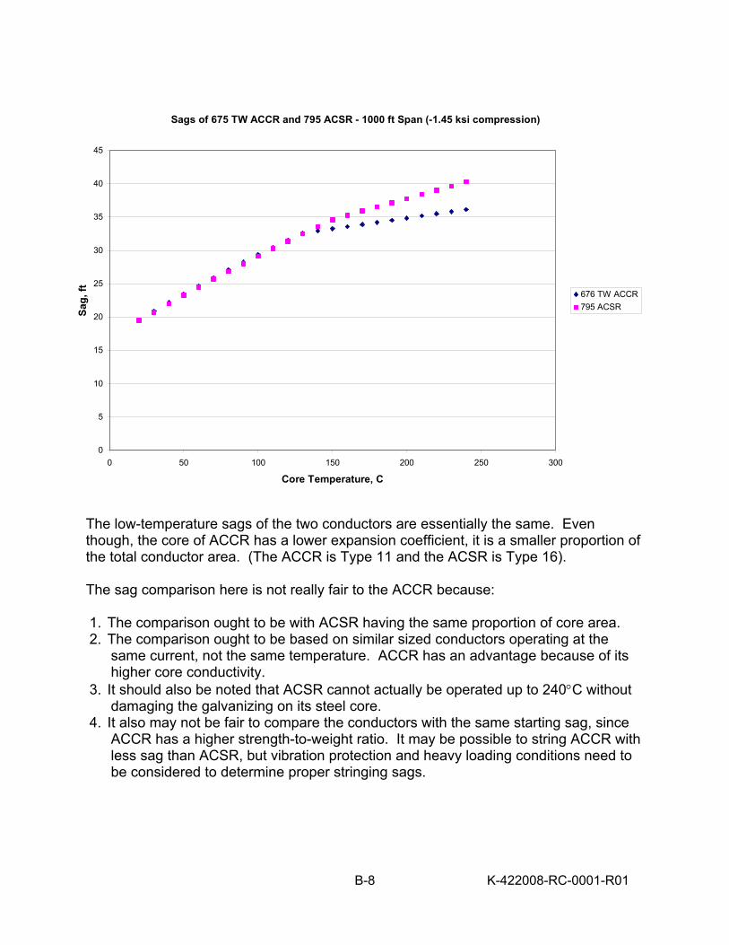
In view of the possibility of larger compressive stresses, depending on conductor manufacture (especially the effect of lay angles), it is recommended to continue using the default value of compressive stress for estimating high-temperature sags. In the present test, the sag at 240°C is overestimated by approximately 1.3 inches. 6) Sag Comparison for a 1000 ft Span The following graph compares the sags of 675TW ACCR with those of 795 ACSR at the same temperatures. These calculated sags are based on a limiting compressive stress of –1.45 ksi in the aluminum at high temperature. The starting sags are matched @ 22°C as they were in the laboratory test, using 2083 kg (4592 lb) for the ACCR and 3152.6 kg (6950 lb). The aluminum stress at 20°C was computed to be 5.7 ksi for the ACCR and 5.6 ksi for the aluminum, which is an indication that they should have similar self-damping characteristics.
K-422008-RC-0001-R01
B-7
Sags of 675 TW ACCR and 795 ACSR - 1000 ft Span (-1.45 ksi compression)
0
5
10
15
20
25
30
35
40
45
0 50 100 150 200 250 300
Core Temperature, C
Sag,
ft 676 TW ACCR795 ACSR
The low-temperature sags of the two conductors are essentially the same. Even though, the core of ACCR has a lower expansion coefficient, it is a smaller proportion of the total conductor area. (The ACCR is Type 11 and the ACSR is Type 16). The sag comparison here is not really fair to the ACCR because: 1. The comparison ought to be with ACSR having the same proportion of core area. 2. The comparison ought to be based on similar sized conductors operating at the
same current, not the same temperature. ACCR has an advantage because of its higher core conductivity.
3. It should also be noted that ACSR cannot actually be operated up to 240°C without damaging the galvanizing on its steel core.
4. It also may not be fair to compare the conductors with the same starting sag, since ACCR has a higher strength-to-weight ratio. It may be possible to string ACCR with less sag than ACSR, but vibration protection and heavy loading conditions need to be considered to determine proper stringing sags.
K-422008-RC-0001-R01
B-8
DISTRIBUTION Dr. Colin McCullough (2) 3M Company Composite Conductor Program 2465 Lexington Ave. South Mendota Heights, MN 55120 USA Mr. C. Pon Kinectrics Inc., KB104